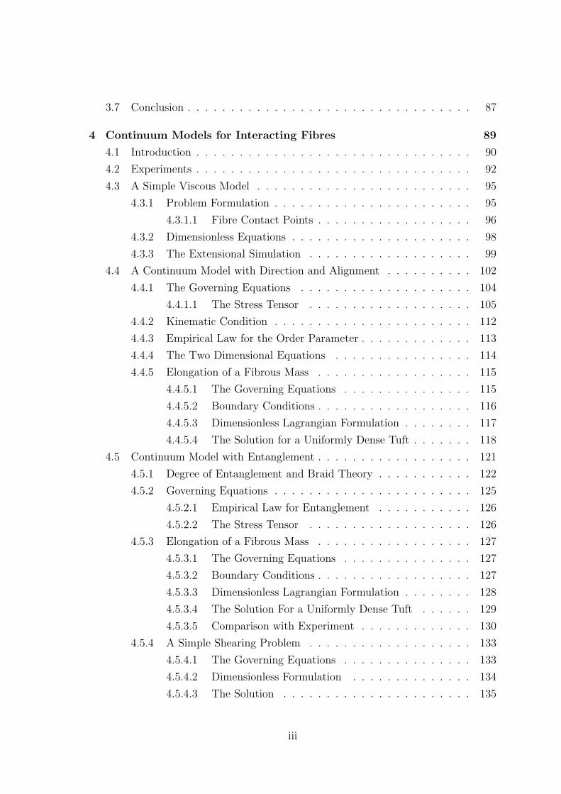
174
Mathematical Models of the Carding Process Michael Eung-Min Lee St. John’s College University of Oxford A thesis submitted for the degree of Doctor of Philosophy Trinity 2001

Mathematical Models
of the
Carding Process
Michael Eung-Min Lee
St. John’s College
University of Oxford
A thesis submitted for the degree of
Doctor of Philosophy
Trinity 2001

To
Luke, Lucy, Daniel and Kylie

Acknowledgements
I would like to thank Dr. Hilary Ockendon, my university supervisor, for
her wisdom, guidance and encouragement over the past three years, and
Dr. Peter Howell, who provided inspiring supervisory assistance for the
second year of my doctoral research. Professor Carl Lawrence, Dr. Abbas
Ali Dehghani-Sanij, Dr. Cherian Iype, Mr. Barry Greenwood and Dr.
Mohammed R. Mahmoudi have been an invaluable source of knowledge
on the carding machine and textile manufacturing. Dr. Marvin Jones
provided lucid discussions on fluid flow in the carding machine and Dr.
Tim Lattimer gave helpful supervisory assistance for the first year of my
doctoral research.
The Engineering and Physical Sciences Research Council generously funded
the interdisciplinary project on carding, from which I was awarded a stu-
dentship.

Abstract
Carding is an essential pre-spinning process whereby masses of dirty tufted
fibres are cleaned, disentangled and refined into a smooth coherent web.
Research and development in this “low-technology” industry have hith-
erto depended on empirical evidence. In collaboration with the School of
Textile Industries at the University of Leeds, a mathematical theory has
been developed that describes the passage of fibres through the carding
machine. The fibre dynamics in the carding machine are posed, modelled
and simulated by three distinct physical problems: the journey of a single
fibre, the extraction of fibres from a tuft or tufts and many interconnect-
ing, entangled fibres.
A description of the life of a single fibre is given as it is transported
through the carding machine. Many fibres are sparsely distributed across
machine surfaces, therefore interactions with other neighbouring fibres,
either hydrodynamically or by frictional contact points, can be neglected.
The aerodynamic forces overwhelm the fibre’s ability to retain its crimp or
natural curvature, and so the fibre is treated as an inextensible string. Two
machine topologies are studied in detail, thin annular regions with hooked
surfaces and the nip region between two rotating drums. The theoretical
simulations suggest that fibres do not transfer between carding surfaces
in annular machine geometries. In contrast to current carding theories,
which are speculative, a novel explanation is developed for fibre transfer
between the rotating drums. The mathematical simulations describe two
distinct mechanisms: strong transferral forces between the taker-in and
cylinder and a weaker mechanism between cylinder and doffer.
Most fibres enter the carding machine connected to and entangled with
other fibres. Fibres are teased from their neighbours and in the case where
their neighbours form a tuft, which is a cohesive and resistive fibre struc-
ture, a model has been developed to understand how a tuft is opened and
broken down during the carding process. Hook-fibre-tuft competitions

are modelled in detail: a single fibre extracted from a tuft by a hook and
diverging hook-entrained tufts with many interconnecting fibres. Conse-
quently, for each scenario once fibres have been completely or partially
extracted, estimates can be made as to the degree to which a tuft has
been opened-up.
Finally, a continuum approach is used to simulate many interconnected,
entangled fibre-tuft populations, focusing in particular on their deforma-
tions. A novel approach describes this medium by density, velocity, direc-
tionality, alignment and entanglement. The materials responds to stress
as an isotropic or transversely isotropic medium dependent on the degree
of alignment. Additionally, the material’s response to stress is a function
of the degree of entanglement which we describe by using braid theory.
Analytical solutions are found for elongational and shearing flows, and
these compare very well with experiments for certain parameter regimes.
5

Contents
1 Introduction 1
1.1 Textile Manufacture . . . . . . . . . . . . . . . . . . . . . . . . . . . 1
1.1.1 The Crosrol Revolving-Flats Carding Machine . . . . . . . . . 3
1.1.1.1 From Feeder-in to Taker-in . . . . . . . . . . . . . . 5
1.1.1.2 On the Taker-in . . . . . . . . . . . . . . . . . . . . . 5
1.1.1.3 From Taker-in to Cylinder . . . . . . . . . . . . . . . 6
1.1.1.4 On the Cylinder . . . . . . . . . . . . . . . . . . . . 7
1.1.1.5 The Doffer . . . . . . . . . . . . . . . . . . . . . . . 8
1.1.1.6 Summary . . . . . . . . . . . . . . . . . . . . . . . . 8
1.1.2 Literature review . . . . . . . . . . . . . . . . . . . . . . . . . 8
1.2 Thesis Overview . . . . . . . . . . . . . . . . . . . . . . . . . . . . . . 14
2 Aerodynamics and Single Fibres 16
2.1 Introduction . . . . . . . . . . . . . . . . . . . . . . . . . . . . . . . . 16
2.2 A Fibre in the Carding Machine . . . . . . . . . . . . . . . . . . . . . 17
2.3 A Mathematical Model for a Single Fibre . . . . . . . . . . . . . . . . 18
2.3.1 Drag on a Fibre . . . . . . . . . . . . . . . . . . . . . . . . . . 18
2.3.2 Internal Fibre Forces . . . . . . . . . . . . . . . . . . . . . . . 20
2.3.3 Aerodynamics . . . . . . . . . . . . . . . . . . . . . . . . . . . 22
2.3.4 Important Parameters . . . . . . . . . . . . . . . . . . . . . . 23
2.4 Fibres on the Cylinder and Taker-in . . . . . . . . . . . . . . . . . . . 24
2.4.1 Rotational Forces . . . . . . . . . . . . . . . . . . . . . . . . . 25
2.4.2 Fluid Dynamics . . . . . . . . . . . . . . . . . . . . . . . . . . 26
2.4.2.1 Annular Flow without Hooks . . . . . . . . . . . . . 27
2.4.2.2 Annular Flow with Hooks . . . . . . . . . . . . . . . 28
2.4.3 The Equations . . . . . . . . . . . . . . . . . . . . . . . . . . 30
2.4.3.1 Boundary Conditions . . . . . . . . . . . . . . . . . . 32
2.4.4 Asymptotic Solution . . . . . . . . . . . . . . . . . . . . . . . 33
i

2.4.4.1 Annular Flow without Hooks . . . . . . . . . . . . . 33
2.4.4.2 Annular Flow with Hooks . . . . . . . . . . . . . . . 33
2.4.5 Numerical Computations . . . . . . . . . . . . . . . . . . . . . 34
2.4.5.1 Annular Flow without Hooks . . . . . . . . . . . . . 34
2.4.5.2 Annular Flow with Hooks . . . . . . . . . . . . . . . 36
2.4.5.3 Friction between and fibre and a hook . . . . . . . . 39
2.4.6 The Doffer . . . . . . . . . . . . . . . . . . . . . . . . . . . . . 40
2.4.7 Summary . . . . . . . . . . . . . . . . . . . . . . . . . . . . . 41
2.5 Transfer Mechanisms . . . . . . . . . . . . . . . . . . . . . . . . . . . 42
2.5.1 Aerodynamics . . . . . . . . . . . . . . . . . . . . . . . . . . . 42
2.5.1.1 From Taker-In to Cylinder (Strong Transfer) . . . . . 45
2.5.1.2 From Cylinder to Doffer (Weak Transfer) . . . . . . 46
2.5.2 Motion of a fibre at a transfer point . . . . . . . . . . . . . . . 47
2.5.2.1 Solutions . . . . . . . . . . . . . . . . . . . . . . . . 49
2.5.3 Frictional Contact Points . . . . . . . . . . . . . . . . . . . . . 51
2.6 Conclusion . . . . . . . . . . . . . . . . . . . . . . . . . . . . . . . . . 52
3 Tufts and Fibres 54
3.1 Introduction . . . . . . . . . . . . . . . . . . . . . . . . . . . . . . . . 54
3.2 The Fibres . . . . . . . . . . . . . . . . . . . . . . . . . . . . . . . . . 56
3.3 The Withdrawal of a Single Fibre . . . . . . . . . . . . . . . . . . . . 57
3.3.1 Constitutive Law . . . . . . . . . . . . . . . . . . . . . . . . . 60
3.3.2 Friction . . . . . . . . . . . . . . . . . . . . . . . . . . . . . . 61
3.3.3 The Equations . . . . . . . . . . . . . . . . . . . . . . . . . . 61
3.3.3.1 Dimensionless Equations . . . . . . . . . . . . . . . . 63
3.3.4 Asymptotic Solutions . . . . . . . . . . . . . . . . . . . . . . . 64
3.3.4.1 Small β Asymptotics . . . . . . . . . . . . . . . . . . 65
3.3.4.2 Small Time Solution for β = O(1) . . . . . . . . . . . 67
3.3.5 Numerical Computations . . . . . . . . . . . . . . . . . . . . . 69
3.4 Teasing out Fibres with a Hook . . . . . . . . . . . . . . . . . . . . . 73
3.5 Tufts held together by a single fibre . . . . . . . . . . . . . . . . . . . 75
3.5.1 The Equations . . . . . . . . . . . . . . . . . . . . . . . . . . 78
3.5.1.1 Dimensionless Equations . . . . . . . . . . . . . . . . 80
3.5.2 Asymptotic Solutions . . . . . . . . . . . . . . . . . . . . . . . 81
3.5.2.1 Small β Asymptotics . . . . . . . . . . . . . . . . . . 81
3.6 Tuft breaking . . . . . . . . . . . . . . . . . . . . . . . . . . . . . . . 85
ii
3.7 Conclusion . . . . . . . . . . . . . . . . . . . . . . . . . . . . . . . . . 87
4 Continuum Models for Interacting Fibres 89
4.1 Introduction . . . . . . . . . . . . . . . . . . . . . . . . . . . . . . . . 90
4.2 Experiments . . . . . . . . . . . . . . . . . . . . . . . . . . . . . . . . 92
4.3 A Simple Viscous Model . . . . . . . . . . . . . . . . . . . . . . . . . 95
4.3.1 Problem Formulation . . . . . . . . . . . . . . . . . . . . . . . 95
4.3.1.1 Fibre Contact Points . . . . . . . . . . . . . . . . . . 96
4.3.2 Dimensionless Equations . . . . . . . . . . . . . . . . . . . . . 98
4.3.3 The Extensional Simulation . . . . . . . . . . . . . . . . . . . 99
4.4 A Continuum Model with Direction and Alignment . . . . . . . . . . 102
4.4.1 The Governing Equations . . . . . . . . . . . . . . . . . . . . 104
4.4.1.1 The Stress Tensor . . . . . . . . . . . . . . . . . . . 105
4.4.2 Kinematic Condition . . . . . . . . . . . . . . . . . . . . . . . 112
4.4.3 Empirical Law for the Order Parameter . . . . . . . . . . . . . 113
4.4.4 The Two Dimensional Equations . . . . . . . . . . . . . . . . 114
4.4.5 Elongation of a Fibrous Mass . . . . . . . . . . . . . . . . . . 115
4.4.5.1 The Governing Equations . . . . . . . . . . . . . . . 115
4.4.5.2 Boundary Conditions . . . . . . . . . . . . . . . . . . 116
4.4.5.3 Dimensionless Lagrangian Formulation . . . . . . . . 117
4.4.5.4 The Solution for a Uniformly Dense Tuft . . . . . . . 118
4.5 Continuum Model with Entanglement . . . . . . . . . . . . . . . . . . 121
4.5.1 Degree of Entanglement and Braid Theory . . . . . . . . . . . 122
4.5.2 Governing Equations . . . . . . . . . . . . . . . . . . . . . . . 125
4.5.2.1 Empirical Law for Entanglement . . . . . . . . . . . 126
4.5.2.2 The Stress Tensor . . . . . . . . . . . . . . . . . . . 126
4.5.3 Elongation of a Fibrous Mass . . . . . . . . . . . . . . . . . . 127
4.5.3.1 The Governing Equations . . . . . . . . . . . . . . . 127
4.5.3.2 Boundary Conditions . . . . . . . . . . . . . . . . . . 127
4.5.3.3 Dimensionless Lagrangian Formulation . . . . . . . . 128
4.5.3.4 The Solution For a Uniformly Dense Tuft . . . . . . 129
4.5.3.5 Comparison with Experiment . . . . . . . . . . . . . 130
4.5.4 A Simple Shearing Problem . . . . . . . . . . . . . . . . . . . 133
4.5.4.1 The Governing Equations . . . . . . . . . . . . . . . 133
4.5.4.2 Dimensionless Formulation . . . . . . . . . . . . . . 134
4.5.4.3 The Solution . . . . . . . . . . . . . . . . . . . . . . 135
iii

4.5.4.4 Comparison with Experiments . . . . . . . . . . . . . 138
4.5.5 An Array of Hooks . . . . . . . . . . . . . . . . . . . . . . . . 138
4.6 Conclusion . . . . . . . . . . . . . . . . . . . . . . . . . . . . . . . . . 139
5 Conclusions 141
5.1 The Life of Fibres in the Carding Machine . . . . . . . . . . . . . . . 142
5.1.1 The Taker-In . . . . . . . . . . . . . . . . . . . . . . . . . . . 143
5.1.2 The Cylinder . . . . . . . . . . . . . . . . . . . . . . . . . . . 143
5.1.3 The Doffer . . . . . . . . . . . . . . . . . . . . . . . . . . . . . 144
5.1.4 Suggested Further Work . . . . . . . . . . . . . . . . . . . . . 144
A Dimensional and Dimensionless Numbers 146
A.1 Drum Speeds . . . . . . . . . . . . . . . . . . . . . . . . . . . . . . . 146
A.2 The Fibres . . . . . . . . . . . . . . . . . . . . . . . . . . . . . . . . . 146
A.3 Fluid Dynamics and Drag . . . . . . . . . . . . . . . . . . . . . . . . 146
A.3.1 Stokes Drag . . . . . . . . . . . . . . . . . . . . . . . . . . . . 147
A.3.2 Taylor Drag . . . . . . . . . . . . . . . . . . . . . . . . . . . . 148
B Shear Breaking Experiments on Tufts 149
C Stability Analysis of a Fibre in the Carding Machine 153
iv

List of Figures
1.1 The two simplified carding process mechanisms: carding and stripping. 2
1.2 A diagram illustrating the points at which high speed photography was
used to examine fibre orientations in the carding machine. . . . . . . 3
1.3 A diagram of the revolving-flat carding machine. . . . . . . . . . . . . 4
1.4 Profile view of a taker-in hook grabbing fibres from the lap. . . . . . . 6
1.5 Plan view of the rotating taker-in hooked surface : snap-shots taken
in numerical order from point I in figure 1.3 of a tuft on the taker-in
(Dehghani et al., 2000). . . . . . . . . . . . . . . . . . . . . . . . . . . 9
1.6 Plan view of the rotating cylinder surface just before the fixed and
revolving-flats: snapshots taken in numerical order from point II in
figure 1.3, of a tuft on the cylinder before the fixed flats (Dehghani
et al., 2000). . . . . . . . . . . . . . . . . . . . . . . . . . . . . . . . . 10
1.7 Plan view of the rotating cylinder surface just after one fixed flat but
before the revolving-flats: snapshots taken in numerical order, from
point III in figure 1.3, of a tuft on the cylinder after one fixed flat
(Dehghani et al., 2000). . . . . . . . . . . . . . . . . . . . . . . . . . . 11
1.8 Snap-shots from point IV, V and VI in figure 1.3, of the regions just
after the point of transfer between the cylinder to the doffer (Dehghani
et al., 2000). . . . . . . . . . . . . . . . . . . . . . . . . . . . . . . . . 12
2.1 A diagram of a single fibre on a rotating drum. . . . . . . . . . . . . 17
2.2 Orthonormal triad of vectors for a fibre’s centre-line. . . . . . . . . . 19
2.3 A rotating cylinder and the local frame of reference for a fibre . . . . 25
2.4 A diagram of the mark V Crosrol Revolving-Flats Carding Machine. . 26
2.5 A diagram illustrating the regions of annular flow. . . . . . . . . . . . 27
2.6 A diagram illustrating annular flow with hooks. . . . . . . . . . . . . 28
2.7 A diagram for annular flow local to a fibre, where both surfaces are
covered in hooks. . . . . . . . . . . . . . . . . . . . . . . . . . . . . . 30
v

2.8 Fibre displacements with a Taylor drag that is induced by shear flow,
where ς = h2ς∗. . . . . . . . . . . . . . . . . . . . . . . . . . . . . . . 34
2.9 A diagram of a fibre in hook entrained flow. The shaded region is very
similar to the problem where there is just shear flow. . . . . . . . . . 36
2.10 The displacement of a fibre with Taylor drag induced by the “triple-
layer” airflow; ς∗ = 0.0005 . . . . . . . . . . . . . . . . . . . . . . . . 37
2.11 A plot of the height of the trailing end of the fibre h plotted against
varying ς, for a fibre with Taylor drag that is induced by shear flow. . 38
2.12 A diagram of the frictional forces between a hook and fibre on a rotating
drum. . . . . . . . . . . . . . . . . . . . . . . . . . . . . . . . . . . . 39
2.13 Displacements for a fibre with Stokes Drag that is induced by a shear
flow, for varying κ . . . . . . . . . . . . . . . . . . . . . . . . . . . . . 41
2.14 A diagram for fluid flow between two rotating cylinders. . . . . . . . 43
2.15 Possible fluid flow topologies between two rotating cylinders. The di-
agrams are in order of increasing ΓDΓC
. . . . . . . . . . . . . . . . . . . 44
2.16 Fluid flow, local to the taker-in, near the point of transfer with the
cylinder. . . . . . . . . . . . . . . . . . . . . . . . . . . . . . . . . . . 46
2.17 Fluid flow, local to the cylinder, near the point of transfer onto the
doffer. . . . . . . . . . . . . . . . . . . . . . . . . . . . . . . . . . . . 47
2.18 A diagram illustrating a two dimensional fluid velocity acting on a fibre. 47
2.19 Fibre displacement on the taker-in moving past the first stagnation
point in the transfer region, see figure 2.5.1.1. As time increases the
angle between the hook and fibre contact point decreases, and the fibre
will slip off the hook. . . . . . . . . . . . . . . . . . . . . . . . . . . . 49
2.20 Fibre displacement near the cylinder-doffer transfer region. . . . . . . 50
2.21 Friction forces acting on a fibre connected to a hook or a couple of hooks. 52
3.1 A diagram of a hook attaching itself to a fibre in a tuft. . . . . . . . . 54
3.2 A diagram of taker-in hooks grabbing a tuft from the lap with inter-
connecting fibres. . . . . . . . . . . . . . . . . . . . . . . . . . . . . . 56
3.3 A diagram of a naturally curved fibre and it’s centre line. . . . . . . . 57
3.4 A diagram of a single fibre being withdrawn from a tuft. . . . . . . . 58
3.5 Possible constitutive relations for tension and strain for a spring or a
crimped fibre. . . . . . . . . . . . . . . . . . . . . . . . . . . . . . . . 60
3.6 Experimental results of a single fibre being withdrawn from a tuft . . 64
vi

3.7 Plot of the force acting on a single fibre being withdrawn from a tuft.
The small β asymptotic solution, where β ranges from 0.01 to 0.1. . . 67
3.8 A single fibre being withdrawn from a tuft: asymptotic solutions for
small time. . . . . . . . . . . . . . . . . . . . . . . . . . . . . . . . . 70
3.9 The computational grid and molecule for a parabolic partial differential
with a free boundary ξ = ξ0. . . . . . . . . . . . . . . . . . . . . . . . 71
3.10 The withdrawal force on of a single fibre: dotted lines plot asymptotic
solutions and the solid lines plot the numerical computations with β =
0.01, 0.02, 0.03, 0.04, 0.05 in ascending order for both sets of results. . 72
3.11 The withdrawal forces on a single fibre. Numerical computations of
force for β = 0.2, 0.4, 0.6, 0.8, 1.0. Plots ascending with respect to β. . 74
3.12 A diagram of a hook teasing a fibre from a tuft; θahook is the length of
contact between fibre and hook, where ahook is the radius of the hook. 75
3.13 A diagram of two tufts with one inter-connecting fibre. . . . . . . . . 76
3.14 The position of the free boundaries, ξ0 and ξ1, for two tufts with an
interconnecting fibre; with varying θ ∈ [0.1, 1] in steps of 0.1. . . . . . 83
3.15 Tension in a fibre between the tufts: the small β problem. The ratio
of length varies in steps of 0.1 in the interval θ ∈ [0.1, 1] . . . . . . . . 84
3.16 The force required to pull two tufts apart held by 10 fibres . . . . . . 86
3.17 Tuft breaking for varying initial gauge lengths: a comparison with
experiment; lU = 1, 1.5, 2, 2.5 . . . . . . . . . . . . . . . . . . . . . . . 87
4.1 A picture of the lap consisting of polyester fibres. . . . . . . . . . . . 89
4.2 Graphs of the tuft breaking force experiment for cotton with variable
elongation velocities. The initial gauge length is 20 mm. . . . . . . . 92
4.3 Graphs of the tuft breaking force experiment with variable initial tuft
lengths: forceweight
plotted against extension (mm). Elongation speed of
50 mm/min. . . . . . . . . . . . . . . . . . . . . . . . . . . . . . . . . 93
4.4 A diagram illustrating the likelihood of contact between a couple of
fibres. . . . . . . . . . . . . . . . . . . . . . . . . . . . . . . . . . . . 97
4.5 A diagram of unidirectional elongation. . . . . . . . . . . . . . . . . . 100
4.6 Solutions for the elongation of a tuft: comparison between experiment
and the simple continuum model. . . . . . . . . . . . . . . . . . . . . 102
4.7 A plan view of the fibre arrangement as they enter the carding machine.103
4.8 A comparison of a couple of 3-fibre bundles with the same average
directionality. . . . . . . . . . . . . . . . . . . . . . . . . . . . . . . . 104
vii

4.9 An illustration of the angle averaged for the order parameter. . . . . 104
4.10 Three distinct states for liquid crystals that can be represented by the
order parameter: φ = − 12, φ = 0 and φ = 1 respectively. . . . . . . . . 105
4.11 A diagram of the stresses acting on a nematic body of fibres and a
randomly orientated body of fibres. . . . . . . . . . . . . . . . . . . . 107
4.12 A diagram illustrating the evolution of the director using kinematics. 112
4.13 A diagram that illustrates the evolution of the order parameter with a
linearly damped rod. . . . . . . . . . . . . . . . . . . . . . . . . . . . 114
4.14 The dimensionless force required to elongate the fibre continuum at
uniform velocity; β = 10 and φ0 = 0. . . . . . . . . . . . . . . . . . . 118
4.15 The dimensionless force required to elongate the fibre continuum; u =5610−3, φ0 = 0 , β = 1 and ν = 0.01. The function with the highest
maximum corresponds to length 0.01 and for increasing gauge lengths
0.02, 0.03 and 0.04, the respective maximum decreases. . . . . . . . . 119
4.16 The dimensionless force required to elongate the fibre continuum; u =5610−3, β = 1 and ν = 0.01. The largest force corresponds to φ0 = 1
and decreases with respect to the order parameter φ0 = 0.8, 0.6, 0.2, 0. 120
4.17 A comparison of two quasi-planar braids with the same order and di-
rectionality. . . . . . . . . . . . . . . . . . . . . . . . . . . . . . . . . 121
4.18 A couple of braid diagrams. . . . . . . . . . . . . . . . . . . . . . . . 122
4.19 A diagram illustrating the product of two braids given in figure 4.18 . 123
4.20 A i-th braid generator and its inverse. . . . . . . . . . . . . . . . . . . 123
4.21 Three couples of braids illustrating transformations that yield the braid
relation. . . . . . . . . . . . . . . . . . . . . . . . . . . . . . . . . . . 124
4.22 Two couples of braids illustrating transformations that yield the far
commutativity relationship. . . . . . . . . . . . . . . . . . . . . . . . 125
4.23 A couple of braids illustrating how extension of an element will intu-
itively reduce entanglement. . . . . . . . . . . . . . . . . . . . . . . . 126
4.24 Results of the dimensionless elongation problem for the continuum
model: (a) and (b) are plots of the order parameter, (c) and (d) are
plots of the entanglement, and (e) and (f) are plots of the force. The
graphs with multiple functions correlate to the given values beneath
the graph in ascending order. . . . . . . . . . . . . . . . . . . . . . . 131
viii
4.25 Results of the dimensional elongation problem for the continuum model:
(a) and (b) compares experiment with mathematical simulation for
varying gauge lengths, (c) and (d) is a comparison for varying velocity.
The functions on each graph correlate to the given values below where
the respective plots in ascending order. . . . . . . . . . . . . . . . . . 132
4.26 A diagram of the shearing problem. . . . . . . . . . . . . . . . . . . . 133
4.27 Results of the dimensionless shearing problem for the continuum model:
(a) a plot of the director, (b) entanglement, (c) and (d) order. The
plots on each graph correlate to the number written below each graph
in ascending order. . . . . . . . . . . . . . . . . . . . . . . . . . . . . 135
4.28 Force graphs for continuum model and the shearing experiment. The
pairs juxtaposed in this figure are simulations and their corresponding
experiment. . . . . . . . . . . . . . . . . . . . . . . . . . . . . . . . . 137
4.29 A diagram of the fibre continuum which is sheared by two arrays par-
allel hooks. . . . . . . . . . . . . . . . . . . . . . . . . . . . . . . . . 138
5.1 Diagrams illustrating the life of a single fibre in the carding machine. 142
5.2 A diagram illustrating the regions where entangled tufts are teased into
individual fibres or evolve into less entangle tufts. . . . . . . . . . . . 144
B.1 Graphs of the tuft shear force experiment for cotton: forceweight
plotted
against shearing distance (mm). . . . . . . . . . . . . . . . . . . . . . 150
B.2 Graphs of the tuft shear force experiment for polyester with variable
speeds: forceweight
plotted against extension (mm). . . . . . . . . . . . . . 151
B.3 Graphs of the tuft shear force experiment for fine wool: forceweight
plotted
against extension (mm). . . . . . . . . . . . . . . . . . . . . . . . . . 152
ix

Chapter 1
Introduction
A few years ago, a group from the School of Textile Industries in Leeds approached the
Oxford Centre for Industrial and Applied Mathematics with the long-standing prob-
lem of understanding fibre dynamics in carding. Although the machines involved have
undergone numerous modifications, predominantly fuelled by the advances in mechan-
ical manufacturing technology, the rudiments behind the process have not changed for
centuries. Furthermore, research and development in this “low-technology” industry
have hitherto depended on empirical evidence. Within a multi-disciplinary group,
including industrialists and experimentalists, we have endeavoured to shed light on
this age-old and fundamental process.
This thesis presents the theoretical aspects of the work accomplished within this
multi-disciplinary research framework. Bespoke mathematical models have been de-
rived for the fibres on three different length scales. The first of the scales models the
motion of a single fibre as it travels through the carding machine. The intermediate
scale focuses on the interplay between fibres and a tuft in order to understand how
fibres are extracted or teased out of tufts. Finally, we consider large volumes of in-
teracting fibres as a continuum, and consider their evolution throughout the process.
These models as a whole give us access to a theoretical simulation that caters for all
areas of the machine at least to a first approximation. We describe the process in
more detail and review the theoretical work done so far and then give a more detailed
overview of the thesis.
1.1 Textile Manufacture
The fundamental operations when manufacturing yarns are carding, drawing, and
twisting. Carding is the process of separating fibres from one another and combing
them to form an ordered even web. Drawing consists of the attenuation of a loose
1

rope of carded fibres into a thinner rope until its thickness is suitable for the insertion
of a twist. Twisting then gives the yarn coherence and some structural stability. The
production processes of different yarns have a great deal in common, in contrast to
the preparation of various textiles for yarn manufacture which is highly dependent
on the chosen material.
Fast
Slow Faster
CARDING STRIPPING
Fast
Figure 1.1: The two simplified carding process mechanisms: carding and stripping.
Most textile materials come to the spinning mill in masses of entangled fibres which
can be described as tufts; the masses may be reduced by various breaking machines,
but before the fibres are spun they must be disentangled and arranged in a smooth
coherent web with uniform density and thickness. The process also incorporates the
elimination of unwanted particles such as vegetation from cotton plants, unwanted
short fibres and soils from wool. One of the negative outcomes of carding is that a
group of fibres may evolve into tightly bound knots called “neps”, which to the yarn
manufacturer are difficult to eliminate and consequently produce discrepancies in the
yarn as they will include noticeable density irregularities.
The manufacturers of textile instruments attempt to create carding tools that
optimise the speed and quality of the process. Modern machines usually consist
of a number of revolving cylinders covered with fine hooks, and in some cases the
cylinders are placed in surroundings that are also covered with hooks. The rudiments
of current methods can be simplified to carding and stripping, see figure 1.1. In the
diagram the fibres are attached to the bottom hooked surface and will interact with
the hooks on the adjacent surface. Carding helps break down tufts by teasing fibres
out of their neighbouring entanglements. Stripping moves fibres from one cylinder
surface to another until it is ready for the next stage of the yarn production process.
Although all the models we shall consider could be applied to all machines in the
2

carding genre, we give a detailed account of a revolving-flat short-staple machine,
which is used to card fibres that are about half a centimetre in length and a micron
in diameter such as cotton, polyester and short wool.
1.1.1 The Crosrol Revolving-Flats Carding Machine
FIXED FLATS
I
IIIII
IV
VVI
TAKER-IN
REVOLVING FLATS
DOFFER
CYLINDER
Figure 1.2: A diagram illustrating the points at which high speed photography wasused to examine fibre orientations in the carding machine.
We begin with a qualitative overview of how a fibre travels through a short-staple
carding machine. A machine is illustrated in figure 1.3. Once the raw materials have
been prepared for yarn production, the fibres are then arranged in a densely packed
entangled array which is called the “lap”. The “taker-in”, sometimes called the
“licker-in”, is the first cylinder that the fibres encounter. When the lap is fed into the
machine, the hooks on the rotating taker-in grab the fibres and carry them towards a
larger drum covered in smaller hooks called the cylinder. All the fibres are transferred
or stripped onto the cylinder. The fibres are then carried by the cylinder hooks into
the carding region. The revolving-flats comb and disentangle the fibres and once they
have been carded they travel towards the final drum called the “doffer”. The transfer
3

SLIV
ER
RE
VO
LV
ING
FL
AT
S
TA
KE
R-I
N
STR
IPPI
NG
CO
MB
ING
& S
TR
IPPI
NG
DO
FFE
R
CY
LIN
DE
R
STR
IPPI
NG
STR
IPPI
NG
RO
LL
ER
CO
MB
ING
LA
P
Figure 1.3: A diagram of the revolving-flat carding machine.
4

of fibres from the cylinder at this point only occurs for a fraction presented to the
doffer hooks. The fibres that have transferred are carried around to a stripping tool
and then exit the machine in the form of a lightly packed and ordered array called
the “sliver”. The other fibres left on the cylinder revolve on its surface until they
reach the doffer transfer region again, and this process is repeated until each fibre
finally transfers onto the doffer. Now we turn to a quantitative and detailed account
of fibres as they travel through a short-staple carding machine.
1.1.1.1 From Feeder-in to Taker-in
Once prepared for yarn production, the entangled fibres or tufts form the disordered
and entangled lap, and for cotton this will typically have around 12,500 fibres per
square centimetre of the lap (plan view). A small roller then continuously feeds the
textile onto the first set of rotating wire hooks, see the left hand side of figure 1.3
and figure 1.4. The orientation of the fibres on the taker-in depends on the level of
entanglement, which form locally connected structures, within the lap and the hook’s
ability to retain fibres as it hits the lap surface. Typically the taker-in hooks or wires
have a front angle 90 and a height of 3.93 mm, and their density on the taker-in
surface is 6.5 per square centimetre, see figure 1.4. There is a millimetre clearance
between the feeder and taker-in hooks and the number of fibres carried onto the
taker-in surface is 18 per square centimetre. On average this means that there are
2-3 fibres per hook, and additionally not a homogeneous spread.
1.1.1.2 On the Taker-in
Figure 1.4 shows the mechanism by which a tuft is teased out of the lap by the taker-in
hooks. The photographs in figure 1.5 are taken just before the fibres reach the taker-
in to cylinder transfer region, point “I” on figure 1.2. We call the cohesive structures
that are composed of fibres, “tuftlets”, and how they are broken down into individual
fibres forms a key part of understanding the carding machine. Dehghani et al. (2000)
give experimental information on the evolution of this population of structures for
some parts of the machine. On the taker-in most tuftlets have a length-to-width
aspect ratio of 1.5, are aligned in the direction of the hooks to within 5, and have a
mean length of 15 millimetres. At this stage of the carding machine, on the taker-in,
when the fibres can be described as individuals or as part of tuftlets, it is estimated by
Dehghani et al. (2000) that about half the fibres are independent of these structures.
It is not clear how to relate the tuftlet-fibre medium on the taker-in with the fibre-
structures inside the lap; for example, individuals could have been teased out of a
5

Clearance
Feeder-in
Taker-in
Angle of Attack
Hook Height
Figure 1.4: Profile view of a taker-in hook grabbing fibres from the lap.
tuftlet in the lap or it could have been an individual in the lap. Dehghani et al. (2000)
were unable to photograph the transfer region due to the constraints of the machine
casing.
1.1.1.3 From Taker-in to Cylinder
The movement of fibres from the taker-in to the cylinder is called drafting and the
amount transferred is traditionally related to the ratio of surface speeds between the
two drums, which is about 2.7 in favour of the cylinder. The cylinder hooks travel
between 35 and 45 metres per second, they are 0.55 millimetres high and have a 63
angle of attack. The hooks on either drum are set with a 0.18 millimetre clearance.
Therefore, the tuftlets are lifted off the taker-in and there is definite elongation caused
by the disparity in surface speed. Figure 1.6 displays pictures taken from point “II”
in figure 1.2, and shows a more elongated or “opened” tuftlet compared to that
in figure 1.5. Dehghani et al. (2000) statistically validate this claim by showing
that tuftlet lengths, aspect ratios and alignment to hook movement all significantly
increase during this transfer region.
The photographic pictures in 1.5 and 1.6 do not aid in understanding how fibres
transfer from taker-in to cylinder, as the transfer regions were difficult to photograph.
Some textiles engineers (Varga and Cripps (1996)) postulate that it is the tail end
6

of the fibre being dragged by the taker-in hook which makes first contact with the
hooks on the cylinder and it is this action that evokes the transfer mechanism. This
claim will be debated in chapter 2.
1.1.1.4 On the Cylinder
Fibres on the cylinder live a complicated life, but we can consider the most important
facets. If we assume that there is a perfect draft from the taker-in this leaves an
average of 7 fibres per square centimetre on the cylinder. As the fibre-tuft medium is
being transported on the surface of this drum at speeds of O(10) metres per second, it
firstly encounters the carding region, which is composed of three fixed flats and then
the revolving-flats, which actually move at the near stationary speed of 10 meters per
hour (relative to the cylinder surface speed), see figure 1.3. The fixed flats have just
under 15 hooks per square centimetre and the revolving flats have around 60. The
wires on the carding surfaces are about 5 millimetres in length and attack the tufts at
75. At point “III” in figure 1.2, after one fixed flat, figure 1.7 shows that tufts still
exist at this point but have undergone substantial changes. In fact Dehghani et al.
(2000) suggest that about 90% of tufts are now aligned to within 5 hook motion,
which is 20% more than the tuftlets on the taker-in. The aspect ratio and the length
of tufts also significantly increase after just one fixed flat. In fact, the deformations in
tuftlet structure may be greater than those measured in the experiment because there
is normally a cloth of fibres on the cylinder that would encourage newly transferred
material to protrude further into the carding hooks, and these were eliminated so as
to minimise unwanted noise in data. Given the substantial changes produced by just
one flat we expect the structures within the tuftlets to be broken down by the end of
the carding region, resulting in a fairly disperse array of fibres.
The other key aspect of the life of a fibre on the cylinder, and in fact the whole
process, is the transfer of fibres onto the doffer. This mechanism is paramount because
the fibrous cloth laid onto the doffer is then stripped and becomes the final product or
slivers that is then transported to the next phase of yarn production. There is little
consensus on the ratio of fibres that transfer and on the mechanism itself. Figure
1.8 displays three photographs: the first shows the region just after the transfer, the
second is a plan view of the doffer and what when lifted off the doffer becomes the
sliver, and the final picture is a plan view of the cylinder after the transfer region.
These photos are taken at point “IV”, “V” and “VI” in figure 1.2.
7

1.1.1.5 The Doffer
Industrialists (Varga and Cripps, 1996) assume that the motion of fibres on the doffer
are unimportant. Fibres are carried around towards the stripping roller which then
extracts all the fibres from the doffer, without significantly changing the structure of
the fibres as they were on the doffer. The fibres as they exit the machine look like
candy floss, predominantly uniform in density and they are certainly less tangled and
more aligned than when they entered the process.
1.1.1.6 Summary
Although there is some useful experimental work, much of the fundamental mecha-
nisms within the machine are still open to debate. How the transfer from one cylinder
to another takes place is one topic of considerable importance, not only for individ-
ual fibres but also for tuftlets. Another vital area of study is the evolution of fibre
structures throughout the machine. Therefore in this thesis we use mathematical
modelling to illuminate our rudimentary knowledge of the carding machine. We pro-
duce novel explanations of the physical mechanisms that include key fibre properties,
machine geometries and hook dimension.
1.1.2 Literature review
There are numerous articles that deal with aspects of the carding machine which are
reviewed in Lawrence et al. (2000) and these are predominantly experimental. Indeed,
there is only a small collection of articles that have attempted to analyse the machine
from a mathematical point of view. A review is given of models that attempt to
simulate the behaviour of fibres during this pre-spinning process and these fall into
two categories, classical mechanics and probabilistic.
Potentially promising work by Roberts Jr (1996) claims to simulate fibre pro-
cessing to the extent that it is near virtual prototyping. The model and the cases
illustrated involved fibre networks that are extruded and transported by a turbulent
free jet and are then electro-statically deposited through a turbulent jet boundary
layer onto a moving conveyer belt. The primary reason for its inadequate description
of the carding process is the fact that hooks are excluded from the problem and the
fibre ensembles are linked together by springs. In section 1.1.1 we see the paramount
importance of hooks and that within the machine there are numerous teasing pro-
cesses that break down fibre ensembles in a non-elastic manner. It is even dubious
whether this model can be applied to other pre-carding opening processes.
8

4
3
2
1
7
5
6
Figure 1.5: Plan view of the rotating taker-in hooked surface : snap-shots taken innumerical order from point I in figure 1.3 of a tuft on the taker-in (Dehghani et al.,2000).
9

6
8
7
5
1
4
3
2
Figure 1.6: Plan view of the rotating cylinder surface just before the fixed andrevolving-flats: snapshots taken in numerical order from point II in figure 1.3, ofa tuft on the cylinder before the fixed flats (Dehghani et al., 2000).
10

7
6
5
4
3
2
1
10
8
9
11
12
13
14
Figure 1.7: Plan view of the rotating cylinder surface just after one fixed flat butbefore the revolving-flats: snapshots taken in numerical order, from point III in figure1.3, of a tuft on the cylinder after one fixed flat (Dehghani et al., 2000).
11

Cylinder and Doffer
Doffer
Cylinder
Figure 1.8: Snap-shots from point IV, V and VI in figure 1.3, of the regions just afterthe point of transfer between the cylinder to the doffer (Dehghani et al., 2000).
12

Smith and Roberts Jr. (1994) and Kong and Platfoot (1997) produce computa-
tional simulations of fibres which are being transported through converging channels
where the forces acting on the fibres are purely aerodynamic. Although converging
channel geometries are important, the aforementioned authors neglect hooks and this,
in conjunction with one of our criticisms of Roberts Jr (1996), we believe to be naive.
Furthermore, fibres within the carding machine are predominantly tethered by hooks
attached to a rotating drum and this has been neglected. Aerodynamic transport
may be important, but they have not explained how fibres transfer from one surface
to another.
Probabilistic methods are employed by Abhiraman and George (1973), Cherkassky
(1994, 1995), Gutierrez et al. (1995), Rust and Gutierrez (1994), Wibberly and
Roberts Jr. (1997), all of whom consider the carding machine as a macroscopic pro-
cess. The fibrous textile material is characterised by density, and the carding action
and transfer regions are replaced by simple functions; density is assumed to decay
exponentially during carding regions and a fraction of the fibres transfer from cylinder
to doffer. The two primary modelling simplifications are to assume that fibre transfer
and carding will redistribute mass at given fixed rates. Each of the aforementioned
authors progress from this basic model in different ways and not surprisingly produce
quite believable results. The main problem with this approach pertains to relating the
parameters in the mathematical models with the machine variables. This means that
the probabilistic approaches adopted by the aforementioned authors are very limited
in terms of their predictive powers when considering advances in machine design and
they do not explain the fundamental mechanisms within the machine.
The mathematical work applied specifically to the carding machine hitherto does
not enlighten a reader who wishes to understand the evolution of fibres and fibre
networks throughout the machine or aerodynamic forces on fibres. Applications of
classical mechanics have been very limited; and the fundamental concepts of fibre-
fibre, fibre-hook interactions and aerodynamic forces acting on fibres have not been
considered. Probabilistic approaches look from a macroscopic view point but they do
not address the crucial issue of how small-scale interactions produce global effects.
Therefore this thesis attempts to outline the underlying physical mechanisms that
govern the evolution of entangled and single fibres within the carding machine.
13

1.2 Thesis Overview
There is a multitude of physics in the carding machine that one could attempt to
model mathematically, and posing relevant and tractable problems is not trivial.
What is clear from the literature review is that there are no obvious starting points.
After many discussions with carding practitioners and textile engineers, we decided
to focus on three distinct areas: single fibres, tufts and fibres, and many fibres. It
is quite conceivable that the whole thesis could have been dedicated to any one of
these three areas. We chose these areas as they were the most pertinent to carding
manufacturers and also posed interesting mathematical problems.
The simplest physical scenario examines how single fibres progress as they are
carried through the carding machine. This assumes that the volume fraction of fibres
is small at least locally. Such a model can be applied in part to the early stages of the
fibre-tuft medium found on the taker-in, since up to half of the fibres can be found
as non-interacting individuals. As the fibres are continually teased out of the tufts
during the carding process, the single fibre approximation becomes more relevant.
We neglect fibre-fibre interactions, and we model the fibre as an inextensible string
with small bending stiffness compared to the external body forces. This follows on
from the seminal work of Taylor (1952), Cox (1970) and Batchelor (1970), who con-
sider hydrodynamic drag acting on bodies with slender geometries. We also consider
rotational and internal forces. There are two distinct geometries that a fibre travels
through, thin annular channels and adjacent rotating drums, and we find the appro-
priate respective fluid flows. Consequently we can determine the displacement of a
fibre throughout the process and therefore study the effect of hook geometries using
static friction laws.
Our work suggests that tethered individual fibres that do not interact with neigh-
bouring fibres, either physically or aerodynamically, should remain close to drum
surface (from which it is tethered) when in thin annular geometries. When individual
fibres approach a neighbouring rotating drum, then we found mechanisms for transfer
onto the next drum. We argue that fibres on the taker-in do not transfer by their
tails first as suggested in Varga and Cripps (1996), and also explain the difference
between taker-in to cylinder and cylinder to doffer transfer mechanisms.
The rest of the work examines how densely packed arrays of fibres are broken
down into single fibres. The first part of this work considers how fibres are teased out
of tufts composed of a uniformly entangled group of fibres and also how tufts can be
broken down. Two cases are described in detail; a single fibre being extracted from a
14

tuft and two separating tufts with interconnecting fibres. The motion of a fibre being
withdrawn from the tuft is assumed not to affect the mechanical integrity of the tuft.
The basic model is derived and a one-parameter family of solutions are found. These
are tested against experimental data from which we can attain values for the respective
parameter. Our conclusion indicates the optimum conditions for extraction, fibre
breakage conditions, and tuft distortion under both shearing, carding and pulling.
This analysis is particularly relevant to modelling tufts and fibre behaviour at the
feeder-in to taker-in, taker-in to cylinder and to a lesser extent the cylinder and
revolving-flats region. Qualitative comparison with experiment, using the model for
two tufts with many interconnecting fibres, are not satisfactory. Therefore, we go onto
consider a model that describes many interacting fibres, where structural changes in
the fibres intrinsically change physical properties of the mass of fibres.
In contrast to the work on single fibres and fibres and tufts, where classical me-
chanics is applied in novel settings, we derive a continuum model that describes the
structure of entangled fibres and their evolution in the carding machine when fibre-
fibre interactions are the dominant forces acting. Motivated partly by the work on
fluid suspension (Hinch and Leal, 1975, Spencer, 1972, Toll and Manson, 1994), we
characterise the material with velocity, density, directionality, and introduce the no-
tion of alignment and entanglement. The model is created specifically for fibres under
tension, and the conjectured governing equations provide a good basis for modelling
evolution in the structure of fibres throughout the carding process. Comparisons with
experiment are promising.
15

Chapter 2
Aerodynamics and Single Fibres
2.1 Introduction
Understanding the life of a single fibre subject to mechanical forces and aerodynamic
drag during the carding process plays an important role in understanding the domi-
nant mechanisms within the machine. We see from photographic evidence in section
1.1 that individual fibres are found throughout the process, where interaction with
other neighbouring fibres either hydrodynamically or through frictional contact points
can be ignored. Our aim is to predict how a single fibre moves through the machine,
therefore it is important to understand the fundamental mechanisms governing its
motion.
We shall work through every aspect of fibre motion that occurs inside the carding
machine, and these can be placed under two fairly general headings, thin channels
and transfer regions. Although the airflow within the machine travels through com-
plicated geometries, and moreover is turbulent in many regions, we use quite crude
mean flow approximations that enable us to highlight important mechanisms. One
criticism of some mathematical models in the literature review of section 1.1.2, not
only macroscopic probabilistic models but also those that consider forces acting on
fibres in the carding machine, such as those of Roberts Jr (1996), Wibberly and
Roberts Jr. (1997) and Rust and Gutierrez (1994), is the lack of insight the models
and their respective solutions give. Our analysis will incorporate hook and machine
geometries, physical fibre properties and machine sensitive aerodynamics.
There are a number of models that will cater for textile fibres that are attached to
the hooks on a rotating drum. By finding the dominant external forces, and balanc-
ing these with the fibre’s internal resistive forces, we find the appropriate governing
equations. This results in the quasi-steady inextensible string equations, driven by
16

either high or low Reynolds number drag. We begin our study by introducing aspects
of the problems that are central to modelling a single fibre in the carding machine.
We find that the geometries within the carding machine play an important role in
calculating the body forces acting on a fibre. There are parts of the machine which
intuitively seem as though they would produce similar forces on a fibre but in fact
produce completely different fibre motion. For example, a fibre will probably remain
on the cylinder whilst in the cylinder-revolving-flats region but may transfer onto the
doffer when presented by the cylinder hooks. Physically, both the aforementioned
scenarios involve similar dynamics and geometries but the fibres behave in very dif-
ferent ways. Such phenomena in the carding machine have not been explained. We
present a model of a general fibre in the carding machine, and we give an aerodynamic
explanation to the aforementioned paradox.
2.2 A Fibre in the Carding Machine
X
Carding Drum
Y
FibreFluid Flow
(relative to drum) Θ
d3
d1
Figure 2.1: A diagram of a single fibre on a rotating drum.
A single fibre moves through the carding machine as a result of being tethered and
dragged by hooks on the rotating drums, see figure 2.1. We can expect the scenario
shown in figure 2.1, on each of the three major drums in the carding machine; the
taker-in, cylinder and doffer. Rotational and aerodynamic forces are bound to affect
a fibre’s displacement, but the relative importance of these effects will depend on
the drag acting on the fibre and the drum’s size and speed. By considering the
friction between the hook-surface and fibre, we may also measure the likelihood that
17

a fibre will slip off the hook from which it is tethered. The neighbouring machinery
may also affect the fibre’s motion throughout the carding process but we shall begin
our calculations by assuming that a fibre is fixed to a hook at a single point and
incorporate machine geometries into the fluid dynamics.
2.3 A Mathematical Model for a Single Fibre
Short wool, polyester and cotton are typical textiles that are carded in short staple
machines. In appendix A.2 we observe that they share a number of physical charac-
teristics, the most obvious being that they all have small aspect ratios, ε = al, where
a is the average diameter and l the average length of a fibre. Therefore, we can
represent a point on the surface of a fibre as
R(s, t) = (X(s, t), Y (s, t), Z(s, t))T + ah(s, t), (2.1)
where (X,Y, Z) represents a point on the centre-line, using s for arclength along
the fibre, t for time and |h| ∼ O(1) represents cross sectional variances. The cross
sectional variances are considered to be small compared to the length of the fibre,
0 < ε 1. For our purposes, R will describe position in a rotating frame of reference
for which R(0, t) is the point at which the fibre is tethered. There are a number of
important fibre attributes: yield and breaking criterion when extended under tension,
the roughness of fibre surface which affects the drag induced by the external fluid flow
and the bending stiffness of the fibre which enables a fibre to keep its natural curvature
or crimp.
2.3.1 Drag on a Fibre
We can take into account varying fibre surfaces in calculating the drag on a fibre.
Cotton and polyester are good examples of the disparity within the micro-structure
of textile fibres; the former is a natural material with a rough hairy surface and
the latter is man-made with a smooth finish. Taylor (1952) obtained experimental
evidence that shows how the texture of a slender cylindrical surface noticeably affects
aerodynamic drag. This empirical work considered incompressible, unidirectional flow
with Reynolds numbers between 20 and 106 based on the radius of a fibre, a, and the
magnitude of fluid velocity, U . In practice the Reynolds number for flow around a
fibre in the carding machine varies between 0.5 and 100. If we consider each rotating
drum within short-staple carding machines separately, the steady state fluid flow is
only dependent on the cylindrical polar radial variable r, the distance from the centre
18

d1 d3
Center-line
d2
Figure 2.2: Orthonormal triad of vectors for a fibre’s centre-line.
of the drum, and is independent of the azimuthal and axial directions of the cylinder.
We neglect the width of a fibre and define an orthonormal triad for each point of
a fibre with respect to the centre line to be (d1,d2,d3), where d1 and d2 are the
principal normals in the cross sectional plane of the cylinder and d3 is the tangent,
see figure 2.2. We make the assumption that the fibre is aligned in the plane of
the unidirectional flow U (r), d2 · U=0. Therefore, we consider a two-dimensional
model for a fibre that will feel drag in the local tangential and normal directions to
its centre-line. Using Θ(s, t) to represent the angle between the fibre’s tangent and
the incoming unidirectional flow, the drag term D per unit length for a smooth fibre
when Re 1 is given by Taylor (1952) as
D =ρairaU
2
2
[(sin2 Θ +
4√Re
sin32 Θ
)d1 +
5.2√Re
cos Θ√
sin Θd3
], (2.2)
where ρair is the density of air and based on our assumption that the velocity of the
fluid flow described in a global Cartesian framework (e1, e2, e3) as U = (U, 0, 0) has
no component in the d2 direction. Equation (2.2) suggests that a straight polyester
fibre, modelled as a smooth cylinder, would not feel any drag when it is aligned parallel
to the direction of the oncoming uniform flow. If we were to consider a natural fibre
which has an approximately cylindrical but uneven surface, the Taylor expression for
drag is
D =ρairaU
2
2
[(sin2 Θ +
4√Re
sin Θ
)d1 + cos Θd3
], (2.3)
Alternatively if the fibre has a hairy surface, then
D =ρairaU
2
2
[4√Re
sin Θd1 + cos Θd3
]. (2.4)
19

We note that for the aforementioned Taylor drags, U ≥ 0 and θ ∈ [0, π2). Highlighting
the differences in aerodynamic drag for varying fibre surfaces, we observe that for both
cases (2.3) and (2.4) when compared to (2.2) the salient difference is the non-zero drag
acting on a fibre that is aligned with the fluid flow.
When the fluid flow around a fibre is “slow”, Re < 1, it would be inconsistent
to use the Taylor approximations for drag. Instead, we use an analytical expression
derived from the Stokes flow approximation for slow viscous fluid dynamics (Keller
and Rubinow, 1976) where the drag to leading order for a smooth fibre is
D =8πρairU
2a
Re log 1ε
(2 sin Θd1 + cos Θd3) . (2.5)
Batchelor (1970) pays attention to small surface variations but this does not affect
the first order terms given in equation (2.5). Other effects such as hydrodynamic
interaction with other fibres and solid boundaries (Cox, 1970, Khayat and Cox, 1989)
also give higher order modifications. Therefore, for drag induced by medium and high
Reynolds numbers we can use the empirical approximation given by (2.3) or (2.4) and
for low Reynolds numbers fluid flow we can use the leading order approximation for
Stokes drag given by (2.5).
2.3.2 Internal Fibre Forces
Most fibres are not straight and polyester is even deliberately crimped in order to
produce more cohesive yarns. We need to consider how a rod which has a surface
described by (2.1) resists external body forces. The resulting equations are derived
from a force balance between external and internal forces. In particular we see that
all the aforementioned drag terms are dependent on the orientation of the fibre Θ,
and it is therefore important to understand the interplay between drag and internal
forces.
Although most textile fibres have bending moduli of the same order of magnitude,
see appendix A.2, their natural shapes can vary considerably. For natural fibres a
distribution of shapes occur due to the conditions during their formation but the
uniform crimp in man-made fibres is regulated by machinery and variances could be
considered to be statistically insignificant. Therefore each fibre will have natural cur-
vature and due to the fact that textile fibres share low yield and breaking extensions,
we begin by treating our cylinder as an inextensible, elastic rod.
There has been much work on the Kirchhoff-Love theory of linearly elastic rods,
sometimes known as elasticas. We give a brief outline of the equations concerned,
20

consequently allowing us to outline the important dimensionless parameters when
considering a fibre in the carding machine. The basis of this theory (Antman, 1995,
Love, 1927) is that extensional and shear deformations are small compared to bend-
ing and twisting and because the fibre is treated as a thin cylinder with a circular
cross section we also neglect the effects of warping. We write down the geometrical
relationship, that the fibre tangent is normal to the cross-sectional plane:
∂R
∂s= d3. (2.6)
We define the stress resultant vector N (s, t) and the couple resultant vector M(s, t)
to be
N (s, t) =3∑
i=1
Ni(s, t)di(s, t), (2.7)
M(s, t) =
3∑
i=1
Mi(s, t)di(s, t), (2.8)
where N1 and N2 are the shear forces and M1 and M2 are the bending moments along
the principal axes of the cross-sectional plane, while N3 is the tensile force and M3 is
the twisting moment. Balancing forces and couples at each cross section in an inertial
frame gives:
∂N
∂s+ F = πa2ρfibre
∂2R
∂t2, (2.9)
∂M
∂s+∂R
∂s∧N = ρfibreI
2∑
i=1
∂2di∂t2∧ di, (2.10)
where F is the external body force per unit length, I = πa4
2is the coefficient of inertia,
and ρfibre is the density of the fibre. To complete the equations (2.9) and (2.10) we
use the Euler-Bernoulli constitutive law, which relates twist linearly with components
of curvature:
M = EI(κ1d1 + κ2d2) +GJκ3d3, (2.11)
E is the Young’s modulus, G is the shear modulus, J is the polar moment of inertia,
and the κi’s are the components of curvature. Equation (2.11) is true for a naturally
straight rod; the moments are proportional to curvature, so in the two limits as the
curvature tends to infinity the moments become singular and when the fibre is straight
there are no moments in the fibre. If a fibre is naturally curved then we would need
21

to alter (2.11) so that there would be no moments in the fibre when in its preferred
natural form.
In order to capture the important terms we derive a dimensionless form to equa-
tions (2.9) – (2.11). Appropriate scalings for each term are:
s = ls, R = lR, κi =κil, F = F F ,
N = lFN , M =EI
lN , t =
l
Ut, (2.12)
where the dimensionless terms denoted by an over-bar are O(1). The typical body
force F represents the size of the drag terms D, which for Taylor drag will be ρairaU2
2
as discussed in section 2.3.1 and for slow flow 8πUµ
log 1ε
, where µ is the viscosity of air.
The equations (2.9) and (2.10) become:
∂N
∂s+ F = Λ1
∂2R
∂t2, (2.13)
∂M
∂s+ Λ2
∂R
∂s∧ N = Λ3
2∑
i=1
∂2di∂t2∧ di, (2.14)
respectively. This results in three important parameters:
Λ1 =ρfibreπa
2U2
lF, Λ2 =
l3F
EI, Λ3 =
ρfibreU2
E, (2.15)
where Λ1 represents fibre acceleration over drag, Λ2 is drag over flexural rigidity and
Λ3 is the torque over elastic modulus; N.B. Λ3 = Λ1Λ2
2ε2.
2.3.3 Aerodynamics
As we have considered the primary forces that will affect the fibre, we now focus
on the external forces, in particular aerodynamics within the machine. Due to the
complexity of the aerodynamics in the carding machine we elect to describe fluid flow
regimes for specific geometries that cover the key areas of process, but there are a few
general features that can be outlined before any particular scenarios are considered.
The air interacting with the fibres will be modelled as a homogeneous incompressible
fluid, and this is accurate if the flow is sufficiently sub-sonic, for example the Mach
number is less than 0.7, see Liepmann and Roshko (1957). The drag on the fibre
depends on the Reynolds number Re, where the length scales of interaction will be
comparable to the diameter of the fibre. The Reynolds number for the flow in general
Redrum, assuming that the hydrodynamic effect caused by fibre motion is negligible,
will depend on the drum size length scales. Therefore as the rotating drums have
22

radii in the order of metres, see appendix A.1, and the single fibres have radii in the
order of microns, see appendix A.2, the Reynolds numbers for flow regimes inside the
carding machine will tend to be six orders of magnitude greater than flow around
a single fibre, see appendix A.3. Consequently, we can expect turbulent or laminar
boundary layers to play an important role in determining the external body force
acting on a fibre.
2.3.4 Important Parameters
PARAMETERS APPROPRIATE APPLICATION
Refibre < 1 Stokes Drag (approximately smooth surfaces only)Refibre > 1 Taylor Drag (dependent on surface roughness)
Λ2 = O(1) and Λ1,Λ3 1 quasi steady elasticaΛ2 1 and Λ1,Λ3 = O(1) unsteady string with no bending stiffness
Λ2 1 and Λ1,Λ3 1 quasi steady string with no bending stiffness
Table 2.1: A table of parameter regimes for a fibre in the carding machine.
This leaves us with a number of parameters that we calculate a priori and in some
regimes, before any serious computation, this will indicate the dominant mechanisms
of fibre transport and will also allow us to simplify the models accordingly. We give
examples of such regimes in table 2.1. The Reynolds numbers around a fibre suggest
the appropriate drag approximations and the Λi’s which may indicate that bending
stiffness, accelerations and torques are negligible. Notice in table 2.1 that we have
not included all possible scenarios, in particular, Λ2 1 is not relevant in practice
and we also neglected significant differences in Λ1 and Λ3 as they would produce less
physically relevant scenarios. We did not include the effect of rotational accelerations
but these can be included in the body forces F in equation (2.9) and (2.13). Now we
are in a good position to begin formulating problems specifically for different areas
of the machine and thence we can write down the respective leading order governing
equations.
We begin the dimensionless evaluation by writing down the approximate magni-
tudes of dimensional quantities, see table 2.2. Then we place the dimensional quan-
tities into the formulae given in (2.15), see table 2.3. The Reynolds number Re, is
given in appendix A.3 for each drum and with the Λi’s we suggest the appropriate
models. Table 2.3 suggests that a fibre in the carding machine can be modelled as a
23

QUANTITY VALUE UNITS
ρair 1.1 gcm−3
µ 1.7 gcm−1s−1
U 0.5-40 ms−1
l 2.5-4 cma 0.5-11 micronE 10 kNmm−2
I = πa4
2150 micron4
Table 2.2: A table of the dimensional numbers for a fibre and air, see appendix A.2.
quasi-steady string. It should be noted that in some cases bending stiffness will be
important, for example near the point of contact with a hook.
DRUM Λ1 Λ2 Λ3 Re MODEL
Taker-In 10−3 104 10−14 10-26 steady string with Taylor dragMain Cylinder 10−3 104 10−14 34-52 steady string with Taylor drag
Doffer 10−5 103 10−9 0.8 - 3.4 steady string with Stokes drag
Table 2.3: A table of the dimensionless parameters and the suitable models for Taker-in, Cylinder and Doffer.
2.4 Fibres on the Cylinder and Taker-in
Using the table 2.3, assuming that Λ1,Λ3 1 and Λ2 1, the approximate governing
equations (2.13) and (2.14), where we now remove the over-bars, reduce to
∂N
∂s+ F = 0, (2.16)
∂R
∂s∧N = d3 ∧N = 0. (2.17)
Equation (2.17), due to the fact that the fibre is to leading order a cylindrical sur-
face, and that we have neglected warping, implies that the stress resultant only has
components in the direction of the tangent, which is the tension and we write N3 = T
so that N = T (s, t)d3. The Bernoulli-Euler equations (2.11) and the force (2.9) and
resultant (2.10) balances for an elastica are derived with the implicit assumption that
the fibre is inextensible (Antman, 1995, Love, 1927). As equation (2.11) is no longer
needed, we use an inextensibility constraint to close the equation (2.16):
d3 · d3 = 1. (2.18)
24
Before we write down the components of equations (2.16), there are two other aspects
that need further consideration in order to determine F : rotational effects caused by
the motion of the cylinder and the fluid flow in the machine.
2.4.1 Rotational Forces
k
iFibre
Rotating Frame
Fixed Inertial Frame
Solid Cylinder
Fluid (air)
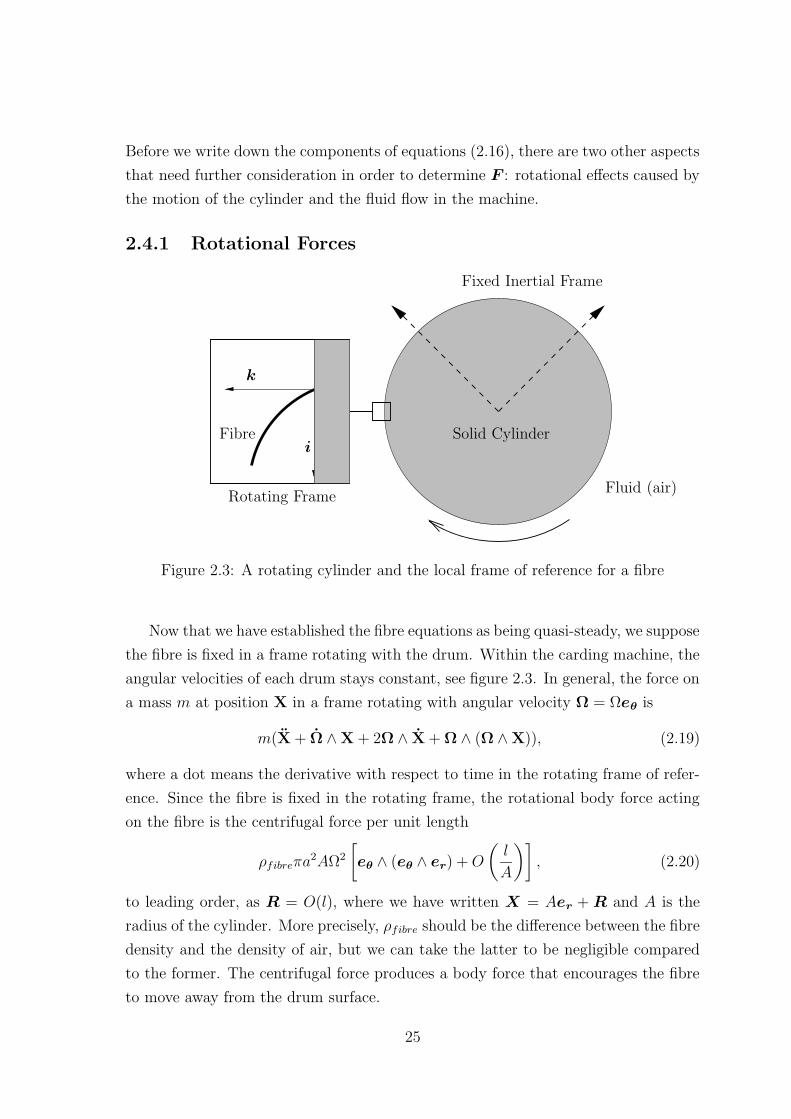
Figure 2.3: A rotating cylinder and the local frame of reference for a fibre
Now that we have established the fibre equations as being quasi-steady, we suppose
the fibre is fixed in a frame rotating with the drum. Within the carding machine, the
angular velocities of each drum stays constant, see figure 2.3. In general, the force on
a mass m at position X in a frame rotating with angular velocity Ω = Ωeθ is
m(X + Ω ∧X + 2Ω ∧ X + Ω ∧ (Ω ∧X)), (2.19)
where a dot means the derivative with respect to time in the rotating frame of refer-
ence. Since the fibre is fixed in the rotating frame, the rotational body force acting
on the fibre is the centrifugal force per unit length
ρfibreπa2AΩ2
[eθ ∧ (eθ ∧ er) +O
(l
A
)], (2.20)
to leading order, as R = O(l), where we have written X = Aer +R and A is the
radius of the cylinder. More precisely, ρfibre should be the difference between the fibre
density and the density of air, but we can take the latter to be negligible compared
to the former. The centrifugal force produces a body force that encourages the fibre
to move away from the drum surface.
25
2.4.2 Fluid Dynamics
DOFFER
CYLINDER
REVOLVING FLATS
FIXED FLATS
MACHINE CASINGFIXED FLATS
MACHINE CASING
MACHINE CASING
TAKER-IN
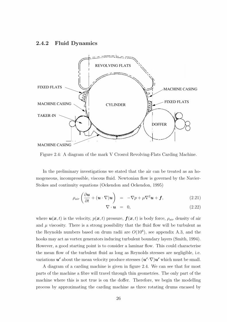
Figure 2.4: A diagram of the mark V Crosrol Revolving-Flats Carding Machine.
In the preliminary investigations we stated that the air can be treated as an ho-
mogeneous, incompressible, viscous fluid. Newtonian flow is governed by the Navier-
Stokes and continuity equations (Ockendon and Ockendon, 1995)
ρair
(∂u
∂t+ (u · ∇)u
)= −∇p+ µ∇2u+ f , (2.21)
∇ · u = 0, (2.22)
where u(x, t) is the velocity, p(x, t) pressure, f(x, t) is body force, ρair density of air
and µ viscosity. There is a strong possibility that the fluid flow will be turbulent as
the Reynolds numbers based on drum radii are O(106), see appendix A.3, and the
hooks may act as vortex generators inducing turbulent boundary layers (Smith, 1994).
However, a good starting point is to consider a laminar flow. This could characterise
the mean flow of the turbulent fluid as long as Reynolds stresses are negligible, i.e.
variations u′ about the mean velocity produce stresses (u′ ·∇)u′ which must be small.
A diagram of a carding machine is given in figure 2.4. We can see that for most
parts of the machine a fibre will travel through thin geometries. The only part of the
machine where this is not true is on the doffer. Therefore, we begin the modelling
process by approximating the carding machine as three rotating drums encased by
26

a solid boundary, see figure 2.5. To simplify the problem we shall consider annular
flow.
2.4.2.1 Annular Flow without Hooks
A
B
Machine CasingFibre
Cylinder
Figure 2.5: A diagram illustrating the regions of annular flow.
If we ignore the resistive forces produced by the hooks, we can find a simple
flow encased by two coaxial cylinders driven by the inner drum’s rotation, see figure
2.5. Using polar coordinates (er, eθ, ez), the unidirectional velocity is prescribed as
u = uθ(r, θ, z, t)eθ, and we look for a steady state ( ∂∂t
= 0), axially symmetric flow
( ∂∂z
= ∂∂θ
= 0), and so the governing equations for the fluid flow (2.22) and (2.21) in
component form become
−ρairu2θ
r=
dp
dr, (2.23)
d2uθdr2
+1
r
duθdr− uθr2
= 0. (2.24)
To accompany the equations (2.23) and (2.24) we impose no-slip conditions on the
inner drum (r = A) with angular velocity Ω and outer (r = B) stationary cylindrical
surface:
uθ = 0 at r = B and uθ = AΩ at r = A, (2.25)
27

and note that the imposition of no-penetration is not required as this condition is
satisfied implicitly through the prescribed azimuthal velocity. The fluid flow is
uθ =ΩA2B2
B2 − A2
(1
r− r
B2
), (2.26)
and the pressure can be found accordingly by integrating (2.23). For the components
in the carding machine B = A + δ, where A = 0.5m and δ = 10−2m, which means
that the velocity profile is approximately Couette flow.
2.4.2.2 Annular Flow with Hooks
AΩeθ
hA hB
A
B
Figure 2.6: A diagram illustrating annular flow with hooks.
To progress onto the next level of sophistication we incorporate a body force on
the fluid that is due to the interaction of the hooks on both the rotating drum and
the outer drum casing. We can use an array of cylinders to describe the hooks, with
radius ahook spaced distance d apart, and that move through the fluid at velocity U .
Based on high porosity
ahookd 1, (2.27)
for fluid moving around the hooks, this produces the body force (Ockendon and
Terrill, 1993, Terrill, 1990):
f = − 4µ%
a2hook
N (%) (u−U ) , (2.28)
28

where % =πa2hook
4d2 1 is the volume fraction of hooks in the fluid and N is a diagonal
matrix, which to O(%) is
N33(%) =1− %
log 1%− 1.476 + 2%
, (2.29)
N11 = N22 =2
(1− %)(log 1%− 1.476 + 2%)
, (2.30)
and this assumes that the hooks are perpendicular to the flow. Notice that the high
porosity condition (2.27) translates to small volume fraction % 1. In fact the
volume fraction of the hooks on the rotating drums and the fixed flats vary between
% = 17
and 110
but for the hooks on the revolving-flats the volume fraction is % = 1100
.
Here the hooks on the outer casing r = B are stationary and protrude a height of hB
and those on the moving inner drum have velocity AΩeθ and height hA, see figure
2.6. This produces the regional body forces:
f =
− 4µ%a2hook
N (%) (u− AΩeθ) when A < r < A+ hA
0 when A+ hA < r < B − hB− 4µ%a2hook
N (%)u when B − hB < r < B, (2.31)
where A+ hA < B − hB. The dimensionless form of the Navier-Stokes, with scalings
u = AΩu, t = 1Ωt, p = ρairA
2Ω2, ∇ = 1A∇ and f = 4µ%N11(%)
a2hook
f , for a steady state
become:
∂u
∂t+ (u · ∇)u = −∇p+
1
Redrum∇2u+ Υf , (2.32)
where Reynolds number is Redrum = ρairA2Ω
µand the hook body force over inertia is
Υ = 4µ%N11
a2hookρairAΩ2 . Typical values for Υ are 102 and as the Reynolds number is high
this means that the effect of the hooks dominate, and therefore we can expect the
flow to be entrained with the carding surfaces. Fluid in between the two regions will
be very similar to the flow in an annulus where the solid boundaries are theoretically
closer. In equation (2.26), the drum parameters A and B can be simply changed to
A+hA and B−hB respectively. So we can model the airflow with a mixture of shear
and plug flow when incorporating hooks into the aerodynamics as shown in figure 2.7,
or more simply we can consider just shear flow. There is no machine casing around
the doffer so a shear flow may be more suitable in this case.
To summarise, we have equations (2.16) and (2.17) for a quasi-steady inextensible
string. The forces that affect a fibre which are produced in the carding machine
environment are aerodynamic and rotational and these can now be included in the
29

governing equations (2.13) and (2.14). Rotation is approximated by a centrifugal
force (2.20) and the drag of the fibre will be given by one of the following equations
(2.3) – (2.5). The drag will also depend on the fluid flow and that will in turn depend
on the machine geometry and dynamics, but the full governing flow equations that
incorporate hooks are given in (2.32).
2.4.3 The Equations
D(Z)
B − A− hA − hB
Cylinder
Revolving-Flats
hB Hook Layer
Shear Layer
Hook LayerhA
fibre
Figure 2.7: A diagram for annular flow local to a fibre, where both surfaces are coveredin hooks.
Channels with hooked surfaces can be found in between the cylinder and the re-
volving and fixed flats, between the taker-in and machine casing and in between the
cylinder and machine casing, see figure 2.4. Without being too concerned with the
regions near transfer between the cylinders, we model the airflow in the aforemen-
tioned channels as above. For the region between the cylinder and fixed or moving
flats both surfaces have hooks, but in the other regions the machine casing is smooth.
From section 2.3, the Taylor drag approximation holds for a fibre on the cylinder
and taker-in and to begin with we choose to model the fibre as cotton, i.e. with a
hairy surface. Although the analysis allows for quasi-steady states for the fibre we are
30

only interested in steady states in the fluid, and this is still consistent with Λ1 and
Λ3 being small compared to Λ2. We find solutions that will give the displacement of
a fibre tethered by a hook and its respective tension. Consequently we can estimate
the amount a fibre will protrude from the rotating drum’s surface and also the forces
acting on the hook-fibre contact point by a static-friction analysis. We find parameter
regimes that will allow fibres to slip off hooks whilst travelling in annular geometries.
Once the drums have attained a steady-state, we can consider the cross planar
forces to be negligible as the there is no component of airflow or rotational forces
across the rotating drums. Due to the fact that the bending stiffness is small, we
can consider a two dimensional model. The aerodynamic modelling in this section
has been based on a unidirectional assumption, so we can write U = U(Z)i where
the global position vector relative to the centre of the cylinder rer = (A + Z)k,
where A is the radius of the cylinder and Z corresponds to the radial component of
the position vector from the surface of the inner drum; we can revert to a Cartesian
frame of reference as the curvature of the drum 1A
is small compared with 1l, making
the region near the fibre to be approximately planar. U(Z) is the approximation
discussed in section 2.4.2 and is shown in figure 2.7,
U(Z) =
ΩA B − A− hB < Z < BΩA Z−hA
B−A−hA−hB hA < Z < B − A− hB0 0 < Z < hA
. (2.33)
Now we can write the equations (2.18) governing the position of the string, where the
forces can now be given explicitly:
∂
∂s(Td3) + Ω2ρfibreπa
2Ak +D(U) = 0 (2.34)
where i and k are global unit vectors, d3 is the tangent vector which can be written
as (cos Θ, sin Θ), and D can be taken from (2.2), (2.3), or (2.4) depending on the
fibre’s surface roughness. Using the scalings (2.12), where tension is scaled with the
product of fibre length and aerodynamic drag, i.e. ρairaA2Ω2
2, equation (2.4) for drag
on a hairy fibre and the inextensibility constraint (2.18) we find that
dT
ds+D(Z(s)) cos Θ + ς sin Θ = 0 (2.35)
dΘ
dsT − 4D(Z(s))
sin Θ√Re
+ ς cos Θ = 0, (2.36)
where over-bars denotes dimensionless variable, D(Z) is the dimensionless magnitude
of the drag and ς =2πaρfibreAρair
is a dimensionless parameter. ς is the ratio of centrifugal
31

force over drag and the values are given in appendix A.3.2. From equation (2.4) the
drag imposed is the square of velocity (2.33), so that
D(Z(s)) =
1 B−A−hBl
< Z(s) < B−Al(
lZ(s)−hAB−A−hB−hA
)2hAl< Z(s) < B−A−hB
l
0 0 < Z(s) < hAl
. (2.37)
If we are to consider the shear flow scenario when hA = hB = 0, the dimensional
velocity function is
U(Z) =ZΩA
B − A, (2.38)
non-dimensionalising so that ς will in this case be2πa(B−A)2ρfibre
Al2ρair, where U ∼ ΩAl
B−A .
We have adopted this different description for ς in the case of shear flow alone as it
allows us to simplify the find a numerical computation, and actual values are given
in appendix A.3.2. Consequently, the drag function becomes
D(Z(s)) = Z(s)2 0 < Z(s) <B − Al
. (2.39)
For consistency we have scaled Z with l although we could have re-scaled with B−A.
To close the system (2.35)–(2.36) we relate the height of the fibre from the in-
ner drum surface Z(s) to the fibre angle Θ(s), by simply writing the geometrical
constraint:
dZ
ds= sin Θ. (2.40)
2.4.3.1 Boundary Conditions
The boundary conditions for the problem with hooks can be posed in a similar way
to the case where there are no hooks and use D as given by (2.39). We assume we
know the point at which the fibre is held to the hook and choose this to be the origin
of the position vector R and the tension at the free end must be zero in order to keep
the applied external forces non-singular. There is one more condition if we are to
pin-point a particular solution and this comes from ensuring that Θ is regular, and
from equation (2.36) at the free end s = 1, we find the appropriate condition. These
three conditions are
T (1) = 0, Θ(1) = arccot4Z(1)2
ς√Re
, Z(0) = 0. (2.41)
32

Imposing a zero tension at the free-end of the fibre will mean that equation (2.36)
becomes singular during numerical computations and so a Taylor expansion from the
end point s = 1 is used to find approximate values close to that end of the fibre:
T (1− ε) = ε4h4 +
√Re ς2
√16h4 +Re ς2
, Θ(1) = arccot4Z(1)2
ς√Re
, Z(0) = 0 (2.42)
when Z(1) = h and where 0 < ε 1. Although h is unknown the approximation is
fine for h ε. We now solve the equations asymptotically and numerically and will
also consider how to solve the problem with the drag that includes the hooks (2.37).
2.4.4 Asymptotic Solution
There are a number of methodologies that can be applied to find solutions to this
problem. Asymptotics can be applied for small or large parameter regimes and nu-
merical computations for all values of ς. We can plot the relationship between the
height of the free-end from the drum surface h against ς. This will indicate the
parameter regimes for which a fibre will interact with other carding surfaces.
2.4.4.1 Annular Flow without Hooks
For airflow without hooks we use equations (2.35), (2.36), (2.39) and (2.40). Asymp-
totic analysis can be employed for small ς which is relevant for the carding machine.
Using a regular perturbation expansion in powers of ς13 for tension T , height Z and
tangent angle Θ, we find that to leading order the fibre is flat, moreover
Θ = Z = O(ς13 ), and T = O(ς
23 ). (2.43)
The next order in the asymptotic expansion requires numerical work, but we can
deduce that the maximum height of the fibre is O(ς13 ). This will also allow us to
assess the gripping powers of a hook if we use a static friction analysis between fibre
tangent at s = 0 and the hook. We have chosen not to document the numerical
calculations for the small ς asymptotic expansions as they are very similar to the full
numerical solutions, see below in section 2.4.5.
2.4.4.2 Annular Flow with Hooks
To incorporate hooks we use the equations (2.35), (2.36), (2.37) and (2.40). We could
think of solving the problem for each of the three regions where different drag forces
are applied by equation (2.37). We would need to prescribe conditions at the interfaces
Z = hAl
and Z = B−A−hBl
, these would be continuity of tension and tangent angle
33

at the interfaces. We shall consider this in more detail when we solve the equations
numerically.
We assume that ς is small and pursue an asymptotic solution in powers of ς13 ,
and find that the leading order solution has constant tangent angle Θ in the lower
entrained region. We then impose continuity of tension and tangent angle at the
interface between the shear layer and the lower hook-entrained region, Z = hAl
. For
the first order problem, the solution cannot have a continuous tangent-angle Θ at
the transition point and so we conclude that the transition point is at the end of the
fibre. A straight line is the first order solution to the fibre’s position from the point
at which it is tethered to the shear-flow interface, and so we write
sin Θ =hAl2. (2.44)
Going to the next term in the expansion we see that only a small fraction of the fibre,
of length O(ς13 ), will be in the shear flow and this will require numerical work. A
static friction analysis will produce a basic calculation for preferred location of the
hook-fibre interface and this follows in section 2.4.5.3.
2.4.5 Numerical Computations
0.2 0.4 0.6 0.8
0.2
0.4
0.6
0.8
1ς∗ = 5
ς∗ = 1
ς∗ = 0.5
ς∗ = 0.1
X
Z
Figure 2.8: Fibre displacements with a Taylor drag that is induced by shear flow,where ς = h2ς∗.
2.4.5.1 Annular Flow without Hooks
Now we look to solve the ordinary differential equations (2.35) and (2.36) numerically
with equation (2.39) for the drag term. We could solve the boundary value problem
34
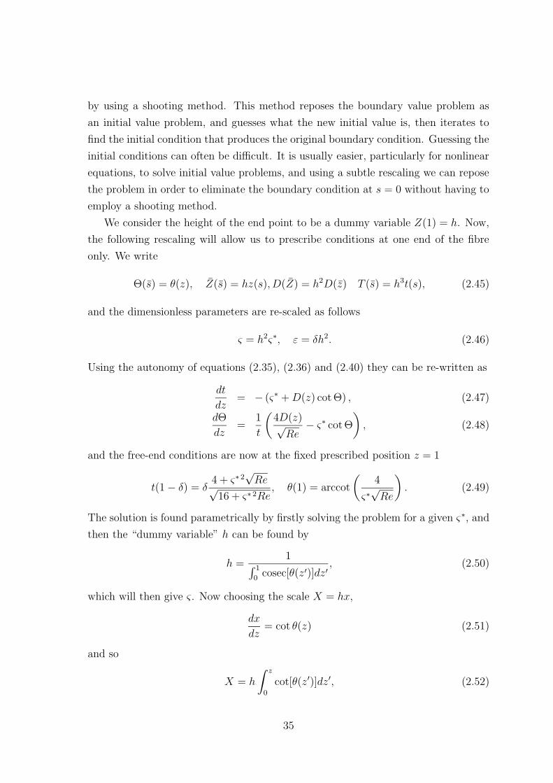
by using a shooting method. This method reposes the boundary value problem as
an initial value problem, and guesses what the new initial value is, then iterates to
find the initial condition that produces the original boundary condition. Guessing the
initial conditions can often be difficult. It is usually easier, particularly for nonlinear
equations, to solve initial value problems, and using a subtle rescaling we can repose
the problem in order to eliminate the boundary condition at s = 0 without having to
employ a shooting method.
We consider the height of the end point to be a dummy variable Z(1) = h. Now,
the following rescaling will allow us to prescribe conditions at one end of the fibre
only. We write
Θ(s) = θ(z), Z(s) = hz(s), D(Z) = h2D(z) T (s) = h3t(s), (2.45)
and the dimensionless parameters are re-scaled as follows
ς = h2ς∗, ε = δh2. (2.46)
Using the autonomy of equations (2.35), (2.36) and (2.40) they can be re-written as
dt
dz= − (ς∗ +D(z) cot Θ) , (2.47)
dΘ
dz=
1
t
(4D(z)√Re− ς∗ cot Θ
), (2.48)
and the free-end conditions are now at the fixed prescribed position z = 1
t(1− δ) = δ4 + ς∗ 2
√Re√
16 + ς∗ 2Re, θ(1) = arccot
(4
ς∗√Re
). (2.49)
The solution is found parametrically by firstly solving the problem for a given ς∗, and
then the “dummy variable” h can be found by
h =1∫ 1
0cosec[θ(z′)]dz′
, (2.50)
which will then give ς. Now choosing the scale X = hx,
dx
dz= cot θ(z) (2.51)
and so
X = h
∫ z
0
cot[θ(z′)]dz′, (2.52)
35
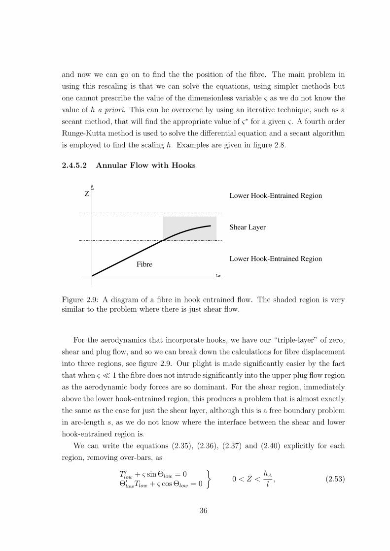
and now we can go on to find the the position of the fibre. The main problem in
using this rescaling is that we can solve the equations, using simpler methods but
one cannot prescribe the value of the dimensionless variable ς as we do not know the
value of h a priori. This can be overcome by using an iterative technique, such as a
secant method, that will find the appropriate value of ς∗ for a given ς. A fourth order
Runge-Kutta method is used to solve the differential equation and a secant algorithm
is employed to find the scaling h. Examples are given in figure 2.8.
2.4.5.2 Annular Flow with Hooks
Z
Fibre
Shear Layer
Lower Hook-Entrained Region
Lower Hook-Entrained Region
Figure 2.9: A diagram of a fibre in hook entrained flow. The shaded region is verysimilar to the problem where there is just shear flow.
For the aerodynamics that incorporate hooks, we have our “triple-layer” of zero,
shear and plug flow, and so we can break down the calculations for fibre displacement
into three regions, see figure 2.9. Our plight is made significantly easier by the fact
that when ς 1 the fibre does not intrude significantly into the upper plug flow region
as the aerodynamic body forces are so dominant. For the shear region, immediately
above the lower hook-entrained region, this produces a problem that is almost exactly
the same as the case for just the shear layer, although this is a free boundary problem
in arc-length s, as we do not know where the interface between the shear and lower
hook-entrained region is.
We can write the equations (2.35), (2.36), (2.37) and (2.40) explicitly for each
region, removing over-bars, as
T ′low + ς sin Θlow = 0Θ′lowTlow + ς cos Θlow = 0
0 < Z <
hAl, (2.53)
36

T ′ +D(Z) cos Θ + ς sin Θ = 0Θ′T − 4D(Z) sin Θ√
Re+ ς cos Θ = 0
hAl< Z <
B − A− hBl
, (2.54)
where Tlow and Θlow are tension and tangent-angle respectively for the part of the
fibre in the lower hook entrained region 0 < Z < hAl
. The interface conditions are
simply continuity as there is no mechanism to support a jump in either Θ or T and
so we add
Θlow = Θ and Tlow = T at Z =hAl
(2.55)
to the boundary conditions (2.42). We note that Z = hAl
corresponds to the fibre
arclength point s = SA, which is not known a priori.
0.2 0.4 0.6 0.8 1
0.1
0.2
0.3
0.4
0.5
hA = 0.5
hA = 0.2
hA = 0.4
x
z
hA = 0.1
hA = 0.3
Figure 2.10: The displacement of a fibre with Taylor drag induced by the “triple-layer” airflow; ς∗ = 0.0005
.
As we have discussed already, the shear layer problem for hAl< Z < B−A−hB
l, is
very similar to the problem that considers Couette flow with (2.39), and we can find
a solution the the shear flow problem replacing ς with ςdum =2πa(B−A)2ρfibre
Al2dumρair, where
ldum is the length of the fibre in the shear layer. Therefore, one way to solve this
problem is to use the numerical simulations obtained by solving equations (2.47) and
(2.48). Then we use the fact that the dimensionless length of the fibre is one, and
37

so we try to find ςdum such that the length of the fibre in the shear layer and the
length of the fibre in the lower entrained region add up to one. Using the interface
continuity condition for Θ we know the angle of the fibre in the lower region as any
uniform θ is a solution for the fibre in the lower hook-entrained region. Therefore, we
can find ςdum such that
hAl sin Θ(0)
+
√2πa(B − A)2
ρfibreAρairςdum
= 1, (2.56)
for which we can employ the secant method. As we have used the same re-scalings of
(2.45) and (2.46), when we solve the equations we find the solution for ς∗dum = h2ςdum.
To find the corresponding ςdum that satisfies (2.56) involves a further root finding
iterative scheme. Examples of fibre profiles are given in figure 2.10 for varying hA.
We see that the fibre barely enters the shear layer. The fibre’s deformation in the
shear layer are the same as those in figure 2.8. We plot the relationship between the
height of the fibres from the drum surface and the dimensionless parameter ς in figure
2.11.
0.002 0.004 0.006 0.008 0.01
0.225
0.25
0.275
0.3
0.325
0.35
0.375
ς
h
Figure 2.11: A plot of the height of the trailing end of the fibre h plotted againstvarying ς, for a fibre with Taylor drag that is induced by shear flow.
38

2.4.5.3 Friction between and fibre and a hook
A fault with the aforementioned model is the presumption that the fibre will not fly
off the hook, and is therefore fixed at one end point. One way to overcome this is
to consider the forces acting on the hook fibre contact point, and we apply static
friction to estimate whether a fibre will move given the fibre’s displacement. Using a
classical static force balance, we can find the conditions for the fibre to slip and this
is illustrated in figure 2.12. In terms of Cartesian components the tension force is
T (0)
(cos[θ(0)]sin[θ(0)]
).
fibre
fibre-hook interface
hook
Drum Surface
ζΘ(0)
N
tangent at s = 0
F
Figure 2.12: A diagram of the frictional forces between a hook and fibre on a rotatingdrum.
If the hook has an angle of attack ζ as in figure 2.12 then in equilibrium the
friction force F and the normal force N are defined as follows,
F = T (0) cos[θ(0) + ζ], (2.57)
N = T (0) sin[θ(0) + ζ]. (2.58)
The fibre will slip if∣∣∣∣F
N
∣∣∣∣ > µs, (2.59)
where µs is the friction coefficient between the hook and the fibre. Then given fric-
tional coefficient µs, we can evaluate the range at which the fibre may be attached to
the hook:
| cot[θ(0)]| > µs. (2.60)
39

This gives us good insight into how the hooks should be designed for the purposes of
keeping the fibre on the hook in the annular regions.
2.4.6 The Doffer
The drum surface speed is an order of magnitude slower on the doffer when compared
to the surface speeds of the cylinder and taker-in. We have previously suggested in
section 2.3 that a quasi-steady inextensible string with Stokes drag (2.5) would be a
suitable model and this approximation is sufficient for a fibre on the doffer. Unlike the
cylinder, the doffer is not surrounded by a casing of hooks or any other mechanical
objects so the flow can be represented by shear flow near the drum surface. It isn’t
clear whether or not the disentangled fibres actually interact with one another here,
but it seems likely from the photographic evidence given by Dehghani et al. (2000).
The fibres once transferred onto the doffer move around the drum surface and are
then stripped off and transported out of the machine. Due to the cylinder moving an
order of magnitude faster than the doffer, the global airflow near the transfer region
will be driven by the fluid entrained by the cylinder. The Reynolds number based
on the doffer’s radius will be O(105) and the high speed photography in section 1.1
suggests that there will be an area of re-circulation just after the transfer region. For
the flow around a fibre, apart from the aforementioned area near the cylinder, fluid
flow near the doffer can be approximated by a cylinder rotating in an infinite fluid
which has a Reynolds number, based on the fibre diameter, of O(10−1). The velocity
field is simplyΩdA
2d
r, where AdΩd is the surface speed of the doffer and close to the
doffer this gives a shear flow approximation for flow relative to the cylinder.
For the fibre itself we derive governing equations in the same way as in section
2.4.3, but now we use the drag formula (2.5) since the Reynolds number for fluid local
to a fibre on the doffer is smaller than unity and this has equations
dT
ds+ κZ cos Θ + sin Θ = 0, (2.61)
TdΘ
ds− 2κZ sin Θ + cos Θ = 0, (2.62)
dZ
ds− sin θ = 0, (2.63)
where κ = 8AdρairaReρfibre log 1
ε
, which is similar to 1ς
but the drag is now based on a Stokes
flow approximation, see appendix A.3.1 for values. These can be solved using the same
asymptotic and numerical approaches used in sections 2.4.4 and 2.4.5 respectively, see
figure 2.13. This predicts the fibre to protrude from the drum surface by the amount
40

1
κ12
and this is usually an order of magnitude greater than ς, which is the amount the
fibre will protrude on the cylinder and taker-in.
0.2 0.4 0.6 0.8
0.2
0.4
0.6
0.8
y
x
κ = 3.0κ = 5.0
κ = 2.6κ = 2.2
κ = 1.8κ = 1.4
κ = 1.0
κ = 0.6
κ = 0.2
κ = 10.0
Figure 2.13: Displacements for a fibre with Stokes Drag that is induced by a shearflow, for varying κ
2.4.7 Summary
All these models, whether the fibre is approximated by shear or triple layered flow, give
evidence that a single fibre will not interact with other machine surfaces, including
hooks on the revolving-flats and any other neighbouring parts of the carding machine.
Although the rotational forces acting on a fibre will project the fibre away from the
surface from which it is tethered, it will not be significant enough so that the fibre
will make contact with other machine parts. This result is still important to those
in the carding industry as there is no consensus on how fibres behave in the annular
regions. The linear stability analysis in appendix C, about a plug flow with velocity
comparable to carding speeds, shows that a fibre will not fluctuate uncontrollably
under the prescribed airflow and rotational forces found in the carding machine. Of
course we have ignored important physics such as the effect of the neighbouring fibres
on both aerodynamics and the fibre itself, and we consider fibre-fibre interactions in
chapters 3 and 4. Therefore, to complete our understanding of the life of a single fibre
in the carding machine we need to postulate a theory for fibre transfer between the
three main drums; taker-in, doffer and cylinder. The dominant body force acting on
41

a fibre is due to aerodynamic drag and we will now consider fluid flow in non-annular
geometries to recognise how fibres transfer between drums.
2.5 Transfer Mechanisms
We have already considered external forces for a fibre in laminar flow in annular ge-
ometries and found that they do not give a transfer mechanism. In section 2.3 we
ascertained the importance of the aerodynamic forces, so we now turn our attention
to the aerodynamics in non-annular geometries. Due to the fluid flow being char-
acterised by high Reynolds numbers when considering scales of motion comparable
with the machine, if the flow is considered to be laminar we can expect predomi-
nantly inviscid flow, Re =∞. Near the machine surfaces we expect boundary layers
of thickness O(
1√Re
). We consider the inviscid case which gives rise to a “strong”
and “weak” transfer mechanism for a fibre travelling in between two rotating drums.
The strong transfer mechanism occurs between the taker-in and cylinder, and the
weak mechanism models the transfer from cylinder to doffer. This coincides with
observation and we find that transfers are not surprisingly dependent on the holding
properties of the hooks, machine geometries, and drum speeds.
2.5.1 Aerodynamics
We are interested in the region between two cylinders of radius rC and rD rotating
in proximity to each other. For simplicity, we consider aerodynamic analysis and
exclude the effects of the hooks and the fibres inside the machine. We consider
two-dimensional incompressible inviscid flow. Then from the continuity equation
(2.22), assuming the flow is irrotational, we introduce a stream function which satisfies
Laplace’s equation:
∇2ψ = 0. (2.64)
This can be solved to give the flow streamlines when applying the appropriate bound-
ary conditions. We prescribe a no-penetration condition which translates to the
stream-function being constant on the given boundary, and this is applied to the
surface of the cylinders’ boundaries. Another interpretation, due to lack of a no-slip
condition, is that any streamline can be a solid boundary and so this means that we
wish to find two neighbouring circular streamlines.
42

Y
X
rc
dt
rd
CDCC
Cylinder C Cylinder D
Figure 2.14: A diagram for fluid flow between two rotating cylinders.
Of course two rotating drums in truly inviscid fluid would not produce any motion,
but because the viscous effects will cause the fluid to rotate we prescribe circulations
around each drum C and D such that:
ΓC =
∮
C
u.dr,
ΓD =
∮
D
u.dr, (2.65)
respectively. This is equivalent to placing a point vortex within each cylinder. The
circulation should then provide a matching parameter for the full viscous problem.
Note that a cylinder, of radius r, rotating in an infinite fluid at any Reynolds number
flow will eventually create a circulation Γ = 2πUr around itself when rotating at
angular velocity U and thus ΓC = 2πuCrC and ΓD = 2πuDrD are plausible values to
take.
There are a number of possible scenarios that can occur as a consequence of
variations in the circulations ΓC and ΓD. There are four possible flow topologies,
two with stagnation points on drum surfaces and two without, an example of each
is illustrated in figures 2.15. We are interested when flow stagnation points can be
found on one of the two drums, as this invokes the transport of fluid from one drum
surface to another, and consequently this may produce the desired transfer of fibres.
43

ΓDΓC
< 0Cylinder C Cylinder D
ΓDΓC
ΓDΓC↑Cylinder DCylinder C
ΓDΓC
ΓDΓC
> 0Cylinder DCylinder C
ΓDΓC
ΓDΓC↑Cylinder DCylinder C
ΓDΓC
Figure 2.15: Possible fluid flow topologies between two rotating cylinders. The dia-grams are in order of increasing ΓD
ΓC.
44

When we consider the circulations to be proportional to the speed of the surfaces of
the carding drums we can expect the magnitude of ΓC to be much greater than the
magnitude of ΓD, where C is the cylinder and D can be either the doffer or taker-
in and this makes the likelihood of stagnation points to be found on D to be quite
probable. Unfortunately it is not really so simple to determine circulations around
each drum, the machine casing and the hook densities on each respective cylinder will
affect the flow topology. Nonetheless, we stay with this simple model and we begin
by outlining the conditions for the four types of fluid flow.
Using a conformal map, Jones (2000a) found that the four flow topologies could
be characterised by the ratio of the circulations
ΓDΓC
, (2.66)
see figure 2.15. Starting with smallest ratio (2.66), a negative one, the circulations will
be in opposite directions and the flow driven around by each drum will not interact
with its respective neighbouring drum surface. Then as we increase the ratios so that
the circulations are in the same direction, the flow will be driven by cylinder C. As
fluid is circulated around C towards the nip region (with drum D) some of the fluid
will go through the nip and some will go around drum D, and in this case there will
be two stagnation points. As we increase the ratio ΓDΓC
the two stagnation points on
drum D move close together until there is only one. Then as we further increase
(2.66), drum D dominates the flow, and the stagnation point moves towards drum C
and once on the surface of the drum will form two stagnation points.
The resulting velocities from this simple inviscid analysis can be used to determine
the external body forces on a fibre, but we can consider much simpler geometries
that still encapsulate the behaviour of fluid flow near the points of transfer. For
the “strong” transfer we consider flow around the cylinder and taker-in where two
stagnation points are on the taker-in. The “weak” transfer consists of flow around
the cylinder and doffer where there are two stagnation points on the doffer. Both the
transfer mechanisms correspond to the second picture in figure 2.15.
2.5.1.1 From Taker-In to Cylinder (Strong Transfer)
We consider the flow near a fibre on the taker-in, where fluid entrained by the cylinder
is driven onto the adjacent drums. We assume that the two stagnation points are on
the taker-in, shown in the second diagram in figure 2.5.1.1, and we can represent the
45
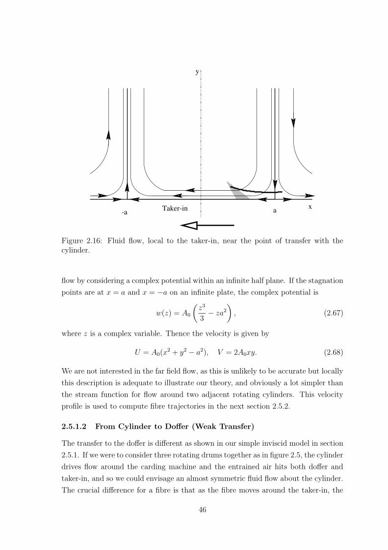
-a a
y
xTaker-in
Figure 2.16: Fluid flow, local to the taker-in, near the point of transfer with thecylinder.
flow by considering a complex potential within an infinite half plane. If the stagnation
points are at x = a and x = −a on an infinite plate, the complex potential is
w(z) = A0
(z3
3− za2
), (2.67)
where z is a complex variable. Thence the velocity is given by
U = A0(x2 + y2 − a2), V = 2A0xy. (2.68)
We are not interested in the far field flow, as this is unlikely to be accurate but locally
this description is adequate to illustrate our theory, and obviously a lot simpler than
the stream function for flow around two adjacent rotating cylinders. This velocity
profile is used to compute fibre trajectories in the next section 2.5.2.
2.5.1.2 From Cylinder to Doffer (Weak Transfer)
The transfer to the doffer is different as shown in our simple inviscid model in section
2.5.1. If we were to consider three rotating drums together as in figure 2.5, the cylinder
drives flow around the carding machine and the entrained air hits both doffer and
taker-in, and so we could envisage an almost symmetric fluid flow about the cylinder.
The crucial difference for a fibre is that as the fibre moves around the taker-in, the
46

hp
Cylinder
Doffer Stagnation Point
Figure 2.17: Fluid flow, local to the cylinder, near the point of transfer onto thedoffer.
surface from which it is being tethered intersects a stagnation point. Once the fibre
is on the cylinder the fibre is dragged around the cylinders axis and then towards the
doffer but in this transfer region the stagnation points are on the neighbouring drum
surface.
A fibre tethered by hooks on the cylinder moves towards the doffer on which
two stagnation points reside. There are several inviscid flow-fields that we could
use to approximate such a fluid flow, for example a block adjacent to a semi-infinite
plane, but we choose a fixed plate which is a height hp from the cylinder surface, see
diagram 2.17. In the high Reynolds number laminar analysis, the leading edge region
is predominantly governed by Euler’s equations that matches onto thin boundary
layers, and we will use this outer-inviscid solution for the drag acting on the fibre
given by Jones (2000b).
2.5.2 Motion of a fibre at a transfer point
Drum Surface
fibre
U (x, y)
i(s)
Θ(s)
Figure 2.18: A diagram illustrating a two dimensional fluid velocity acting on a fibre.
47

From section 2.3, we can treat the equations for dynamic fibre motion as quasi-
steady. Unlike section 2.4, here it would be inconsistent to incorporate the rotational
forces as they are smaller than accelerations in an inertial frame. The equations we
solve are still (2.16) and (2.17) but the only variant is that the velocity is no longer
unidirectional and therefore a little care is needed to re-write the equations as we
have two components in the velocity, see figure 2.18. From section 2.3, we will use
the Taylor drag given for a hairy surface given by (2.4), as opposed to Stokes drag,
as the fibre will be most affected by the fluid driven by the cylinder, since Re based
on the cylinder speed is O(10).
The fibre equations now incorporate a general fluid velocity U (x, y) = (U, V ).
Taylor drag approximations are based on uniform flow around cylindrical shaped
bodies. The fibres can be arranged so that the flow hits the fibre at oblique angles,
which due to the simplicity of the flow on previous occasion we related simply with
the fibre angle Θ(s) but now as the angle varies we write the angle of attack as
i(s) = Θ(s)− arctanU(x(s), y(s))
V (x(s), y(s)), (2.69)
see figure 2.18. The dimensionless governing equations now read:
dT
ds+ (U(X,Z)2 + V (X,Z)2) cos i = 0, (2.70)
TdΘ
ds− 4√
Resgn(i)(U(X,Z)2 + V (X,Z)2) sin i = 0, (2.71)
dX
ds− cos Θ = 0, (2.72)
dZ
ds− sin Θ = 0. (2.73)
It remains to apply boundary conditions and these are very similar in essence to
(2.41), i.e. no tension at the free end, and spatial conditions for the end of the fibre
that is being tethered,
T (1− ε) ∼ (U 2 + V 2)ε, (2.74)
X(0) = Xhook, (2.75)
Z(0) = Zhook, (2.76)
but the angle of the free end Θ(1) needs to be found by solving the equation
sin i(1) = 0. (2.77)
(2.78)
This leaves us with a fourth order system of coupled ordinary equations (2.70)-(2.73)
with four boundary conditions.
48

2.5.2.1 Solutions
0.6 0.8 1.2 1.4 1.6 1.8
0.02
0.04
0.06
0.08
Time
Z
X
hook-fibre contact point
Taker-in
Stagnation point at a=1
a hook
Figure 2.19: Fibre displacement on the taker-in moving past the first stagnation pointin the transfer region, see figure 2.5.1.1. As time increases the angle between the hookand fibre contact point decreases, and the fibre will slip off the hook.
In formulating the numerical solution we cannot use the same rescaling as we did
in section 2.4.5, as this relies not only on the autonomy of the differential equations
but also on one spatial variable, in that case Z. Now that the velocity depends on X
and Z a rescaling is not so simple nor is it as intuitive. Instead, we use a shooting
method, guessing two conditions at one end of the fibre where the other two remaining
conditions are given a priori. We choose the spatial conditions
X(1) = Xend, Z(1) = Zend (2.79)
to be the shooting parameters. Then a Runge-Kutta discretisation is used to compute
the solution to the given system of ordinary differential equations.
49

-1 -0.5 0.5 1 1.5 2
0.2
0.4
0.6
0.8
1Fixed Plate (Doffer)
X
Z
Cylinder Surface
(a) fibre of dimensionless length 1
-0.5 0.5 1 1.5 2 2.5 3
0.2
0.4
0.6
0.8
1
X
Z
(b) fibre of dimensionless length 2
Figure 2.20: Fibre displacement near the cylinder-doffer transfer region.
For the taker-in to cylinder region, where airflow in section 2.5.1 predicts that
there will be stagnation points on the taker-in, the fibre as it reaches the first stag-
nation point may slip down the fibre as air from the cylinder flows onto the taker-in,
see figure 2.5.1.1. On either side of the first stagnation point, the fluid moves in op-
posite directions. When the fibre moves past the stagnation point drag on the fibre,
either side of the stagnation streamline, will compete against each other and this will
probably keep the fibre tethered to the hook. When approximately half the fibre is
either side of the first stagnation point the airflow drags the textile off the hook, see
figure 2.19. The fibre, now free, aligns itself to the flow Hinch (1976). Then the
fluid transports the fibre towards the second stagnation point from which the fibre
50

is carried away from the surface of the taker-in onto the cylinder. It is difficult to
envisage a scenario where a fibre can remain on the taker-in, even regardless of hook
dimensions and holding properties.
When we consider a plate above an infinite half plane, this describes local be-
haviour in the cylinder to doffer transfer region. In figure 2.20, we see quasi-steady
animations of a fibre that moves underneath the stagnation point. We note that the
hooks on the doffer will typically be found in the region 0.2 < Z < 1 on the plots
in figure 2.20, and so in both cases shown there will be a good chance of interaction
with the doffer-hooks. These hooks are the largest in every dimension of all the hooks
found in the carding machine, and as the drum hooks are made of similar materials
the frictional holding forces will be greater.
In the case where the fibre is double the length keeping all other parameters
fixed, plotted in (b) of figure 2.20, the tail end rises to touch the surface of the fixed
semi-infinite plate or the doffer, which may encourage slip at the cylinder-hook-fibre
contact point, and this is due to aerodynamic forces alone. Alternatively the rising
fibre of longer length may attach itself more convincingly to a hook on the upper
surface. To complete the study of the transfer mechanics we need to understand the
inter-play between the dimension of the hooks involved and the frictional resistance
caused by hook-fibre contact points.
2.5.3 Frictional Contact Points
There are three possible ways in which a fibre may slip off the hook from which it is
being tethered. The first we consider is when a fibre is held by two hooks and slips
off the end of one. We can apply a fairly simple frictional analysis (Baturin, 1964)
that indicates which hook will retain the fibre, see figure 2.21, picture (a). Assuming
the fibre is approximately parallel to the drum surfaces, a condition for slipping is
cos Θ1 + µc sin Θ1 > cos Θ2 + µd sin Θ2, (2.80)
where µc,d are the frictional coefficients between the fibre and hooks on the cylinder
and doffer. The fibre will stay on the bottom cylinder and when (2.21) is not satisfied
the fibre will transfer onto the doffer. There are two other possibilities for a fibre to
transfer from cylinder to doffer. The first is when a fibre is removed from a hook
purely by aerodynamic forces as described in section 2.4.5.3 and we can use the same
inequality (2.59)∣∣∣∣F
N
∣∣∣∣ > µs.
51

Cylinder
R
S1
S2
U1
U2
Θ1
Θ2
(a) Profile with two hooks.
Cylinder
Fibre
Hook
(b) Profile with one hook.
Fibre
Cylinder Hook
Doffer Hook
(c) Plan with two hook.
Figure 2.21: Friction forces acting on a fibre connected to a hook or a couple of hooks.
The second is when one part of the fibre is dragged around and off one hook as shown
in picture (c) of figure 2.21. For this case, we can assume the fibre held between the
two hooks will stay on the cylinder if the following inequality is satisfied,
µca2c > µda
2d, (2.81)
where ac and ad are the radii of the cylinder and doffer hooks respectively. Inequality
(2.81) is a rather simple approach that approximated the hook cross sections to be
circular, but even if this is not sufficient for some, the reader can envisage, certainly
for this case, that the relationship will depend on hook architecture and in particular
the surface contact. We have three conditions from the inequalities (2.59), (2.80) and
(2.81), and these are not necessarily mutually exclusive.
2.6 Conclusion
We began the work on a single fibre by considering what internal and external forces
are important, as well as how machine geometries may affect the modelling process.
52

Subsequently we found that a fibre that is dragged through air travelling at speeds of
30 metres per second, in a rotating frame of reference, would approximately behave
as a quasi-steady string; the fibres bending rigidity and the centrifugal forces were
dwarfed by aerodynamic drag.
It was clear that when considering flow in thin annular geometries, a fibre would
remain close to the body of the rotating drum. It was also shown that a fibre is linearly
stable in a plug flow. Therefore, we predict that single fibres tethered by hooks on
any of the carding drums do not interact with neighbouring machine surfaces, such as
the flats. This however did not enlighten us on how a fibre moves between cylinders,
as the reach of the hooks on adjacent drums or in other carding machinery such as
the revolving flats are similar. Fluid flow was the dominant external body force and
for the velocities in the channels we studied there was no normal component to the
flow. This led us onto consider different flow geometries.
An inviscid analysis allowed us to consider flow regimes between adjacent drums.
We concluded that stagnation flows may well give rise to a transfer mechanism. The
flow in the carding machine will be predominantly driven by the air entrained by the
cylinder. This suggested that there are stagnation points on both doffer and taker-
in. We discovered that if a fibre is tethered to the drum on which the stagnation
points are this will invoke a “strong” transfer mechanism, forcing all fibres to migrate
onto the neighbouring drum. When the stagnation points are on the surface of the
other neighbouring drum then this will invoke a “weak” transfer mechanism. In the
latter case, “weak” transfer, the fibres will not necessarily transfer as it will depend
on whether significant parts of the fibre will make contact with the hooks on the
neighbouring surface. If the fibre connects well with a hook, we outlined three possible
contests that neighbouring hooks would undertake in order to retain or obtain the
respective fibre.
For the transfer mechanisms, the next stage would be to include viscous fluid
mechanics as these may affect the possible flow topologies found near the respective
transfer regions. Another additional level of sophistication, that can be applied to
both models, would be to consider a semi-dilute suspension where fibres interact
with each other and this is considered in the next two chapter. Nonetheless we
have postulated a sensible theory to this age-old mystery of how a fibre behaves in
the carding machine and hopefully dispelled the myth that fibres from the taker-in
transfer onto the cylinder by their trailing ends.
53

Chapter 3
Tufts and Fibres
Figure 3.1: A diagram of a hook attaching itself to a fibre in a tuft.
3.1 Introduction
The fibre withdrawal problems presented in this chapter are motivated by the study
of tufts within the carding machine. Photographic evidence, given in section 1.1 from
work by Dehghani et al. (2000) supports the hypothesis that tufts can be found on
the taker-in and cylinder. More specifically, it is found that about 50% of the fibres
on the taker-in and on the cylinder before interaction with revolving and fixed flats
are in tufts and the other 50% are laid down as individual fibres. During the carding
process, tufts are broken down into individual fibres by the time they arrive at the
cylinder-doffer transfer region. This is predominantly a consequence of the carding
54

action between the cylinder hooks and the revolving-flats, but part of the teasing
process occurs when taker-in hooks attack the entangled fibres entering the machine
via the feeder-in, see figure 3.1, and again at transfer from taker-in to cylinder. From
the point of entry into the carding machine, fibres are being continually teased away
from a cluster of neighbouring fibres or tuft, therefore in this chapter we examine the
inter-play between fibre and tuft.
Within the carding machine, when a hook moves through a tuft there are a few
possible outcomes. The hook may:
• move through the tuft without changing the orientations of the fibres a great
deal.
• attach itself to a single fibre, either extracting the fibre completely or leaving
part of the fibre extruding out of the original body of fibres, see figure 3.1.
• attach itself to many interconnected fibres, breaking down the original tuft into
two tufts, see figure 3.2.
We model each case with the exception of the unaffected tuft. These scenarios are
likely to occur when the taker-in hooks grab fibres from the lap in the transfer region
between feeder-in and taker-in, taker-in and cylinder, and to a lesser extent between
cylinder hooks and revolving-flats’ hooks, see figures 3.1 and 3.2.
Firstly, we describe the model for a single fibre that is withdrawn from a tuft.
Although this is not directly applicable to the carding machine it does correspond
to an experiment completed by the School of Textile Industries which allows us to
validate the modelling assumptions and estimate some of the parameters. A natural
extension to the extraction of a single fibre from a tuft is to consider a hook that
attaches itself to a fibre where both ends of the fibre are in the material, see figure
3.1. We go onto consider how tufts are broken down and we do this by modelling a
single tuft, that is being extended, and evolves into two discrete entities connected
by n individual fibres, see figure 3.2.
Therefore we address the key fibre-tuft problems that are relevant to the carding
machine. Once we find the tension, because our fibres are treated as unbreakable and
therefore no breaking stress is prescribed a priori, we can approximate the point in
the simulation where breakage occurs. The control of breakage is paramount for the
production of good quality yarns. The idea behind all our applications in this chapter
is based on the extraction of an inextensible single thread from a material that is on
average a uniform continuous media.
55

LAPTAKER-IN
TUFT
Figure 3.2: A diagram of taker-in hooks grabbing a tuft from the lap with intercon-necting fibres.
3.2 The Fibres
The fibres found in the textiles industry have fairly low breaking extensions, for
example 7% for polynosic viscose and high tenacity polyester, and 5%–10% for cotton.
For the vast majority of textile fibres, yield strains occur when fibres are extended
approximately 1%; that is, a fibre will deform elastically up to this point. Due to the
low yield strain and breaking extensions for the materials concerned we will focus on
the stresses acting on a naturally curved or crimped, inextensible fibre with bending
rigidity.
Man-made fibres such as polyester are uniformly crimped, for example a fibre
that is 3 centimeters long may have around 10 uniformly distributed turning points.
Many natural fibres such as cotton have non-uniform curvature, and there may be
a few scales on which turning points occur. A simple way to view the extraction
of a fibre from a tuft is to consider a straight line between the two ends, see figure
3.3, and model the fibre as a spring lying along this line. Note that the fibre-centre
line, due to crimp or natural curvature will be two to three times shorter than the
length of the fibre itself and this means that the straight line representing the fibre
will be extensible although the fibre itself is inextensible, see figure 3.5. Work by
Cooke (2000) examined models for a crimped fibre under tension and showed that
56

the tension-extension relations were linear for small tension and tended to a fixed
maximum extension as the tension increased. We examine this in more detail when
we derive the equations in section 3.3.
Figure 3.3: A diagram of a naturally curved fibre and it’s centre line.
Tufts are composed of many fibres that are entangled, forming a cohesive structure
due to their intrinsic topological arrangement. When a body force is applied to the
tuft, resistance is due to friction generated by the fibre-fibre contact points. If we
apply a force to the end of a fibre, extracting it from the tuft, the motion of the
fibre will be constrained by the geometry of its neighbours. This is similar to the
concept of reptation in the theory of polymers for dense arrays of long-chain molecules.
Although the topologies and densities may change throughout the tuft, we treat it
as a homogeneous material, which is an adequate assumption for dense materials.
Consequently we focus on the stress in the fibre that is being extracted and assume
there are no deformations in the tuft from the deformations in the fibre. The typical
dimensions of the tuft that we consider should be greater than the length of a fibre’s
centre-line. Finally we assume that when a fibre is extracted from the tuft, this does
not significantly affect the physical properties of the tuft itself.
3.3 The Withdrawal of a Single Fibre
Figure 3.4 illustrates the geometry of our model. The point at y = 0 is the interface
between the tuft boundary and the air. The vertical line at x = 0 represents the
centre-line of the fibre and y ∈ (0, D(t)) is the part of the fibre extending out of the
tuft and y ∈ (−h(t), 0) is part of the fibre embedded in the tuft. Movement in the
boundary of the tuft is assumed to be negligible as we do not expect the movement of
57

Fibre
y=D(t)D(t)
h(t)
Centre lineFibre
TUFT
AIR
F(t)
y=0
y=-h(t)
Figure 3.4: A diagram of a single fibre being withdrawn from a tuft.
a single fibre to significantly affect the orientation of the tuft. For the part of the fibre
in the tuft there is a force acting on the surface of the fibre that is due to dynamic
friction. Outside the tuft we ignore the effect of drag caused by the air. Gravity is
ignored throughout the problem.
We will apply a withdrawal condition at the end point and this consists of either
prescribing the velocity, D(t), or the force, F (t). In our case it is useful to prescribe
velocity as we wish to compare mathematical simulation with experiments. Further-
more in all carding machine scenarios, a hook will move approximately at a constant
velocity through a tuft. Using an Eulerian description, denoting T as tension and y
as the fibre length variable, we find the global force balance:
T (y, t) = F (t) for 0 < y ≤ D(t), (3.1)
∂
∂yT (y, t) = f for −h(t) < y < 0, (3.2)
where f is the resistance per unit length to motion caused by the inter-fibre contact
points. As there are no forces acting on the fibre when y ∈ (0, D(t)) we consequently
have the simple form for tension (3.1). It remains to impose the boundary conditions
and also the constitutive equations for the fibre. At the end of the fibre in the tuft
58

there will be no tension, at the tuft-air interface the tension is continuous, and initially
before the fibre is withdrawn from the tuft there will be no tension in the fibre, and
so these conditions correspond to
T (y, t) = 0 at y = −h(t), (3.3)
T (y, t) = F (t) at y = 0, (3.4)
T (y, t) = 0 when t = 0, (3.5)
respectively. At the moment we choose to prescribe D(t), the rate of withdrawal, but
this means that F (t) the tension in the string in the air, and −h(t) the depth of the
fibre inside tuft, are unknown.
To complete the system we need to relate strain with stress in the fibre but before
we go on to explain the possible constitutive relationships we change the coordinate
system to a more intuitive framework, namely Lagrangian variables ξ and t. In
a Lagrangian description we follow elements of the fibre centre-line and this is a
natural system to work in, particularly when considering elastic deformations. We
define ξ = y + h(0) at t = 0, where for a fibre of length l, ξ = l is the end from
which the fibre is withdrawn from the material, and ξ = 0 is the trailing end inside
the tuft. Our spatial coordinate system is now bound by the fibre end points 0 and
l. The tuft-air interface moves relative to the fibre elements and we define this point
as ξ = ξ0(t). The Eulerian coordinates transform to the Lagrangian framework as
follows:
y = D(t) 7→ ξ = l, (3.6)
y = 0 7→ ξ = ξ0(t), (3.7)
y = −h(t) 7→ ξ = 0. (3.8)
The position y can now be written as a function of time and element, i.e. Y (t, ξ),
and then the velocity is ∂Y∂t
and Y (0, ξ) = ξ − h(0). To complete the Lagrangian
transformation we must map the field equations from (3.1) and (3.2) to
T (ξ, t) = F (t) for ξ0(t) < ξ ≤ l, (3.9)
∂ξ
∂Y
∂
∂ξT (ξ, t) = f for 0 < y < ξ0(t), (3.10)
where ∂ξ∂Y
= 1∂Y∂ξ
. The boundary and initial conditions, (3.3)–(3.5) become
T (ξ, t) = 0 at ξ = 0, (3.11)
T (ξ, t) = F (t) at ξ = ξ0(t), (3.12)
T (ξ, t) = 0 when t = 0, (3.13)
59

respectively.
3.3.1 Constitutive Law
With the introduction of the Lagrangian variable, we are in a good position to define
a plausible constitutive relationship:
∂
∂ξY (ξ, t) = Φ
(T (ξ, t)
k
)(3.14)
where k is the elastic modulus or spring constant. For Φ, we expect linear elasticity to
hold where one applies Hooke’s Law for small stresses. When the string is extended
fully at tension greater than Tc then Φ is constant, which means the fibre has been
extended fully. Thus a simple choice for Φ is
Φ(T ) =
1 + T 0 < T < Tc1 + Tc Tc < T
. (3.15)
Alternatively for a smoother transition near the point where the fibre is fully extended
we could use Φ(Tk
)= 1 + (Tc − 1) tanh T
k, see figure 3.5. We note that regardless of
1
Φ
Tck
Tk
Figure 3.5: Possible constitutive relations for tension and strain for a spring or acrimped fibre.
the choice of Φ, the condition Φ(0) = 1 must be satisfied, which simply ensures that
when there is no tension in the string there is no extension and the fibre remains in
its natural state.
60

3.3.2 Friction
The discrete contact points in a dense tuft are approximated by a continuous surface
force on the fibre. The classical laws attributed to Coulomb and Amonton state that
static friction between two objects is independent of the surface area of contact and
is proportional to the normal force between them. Coulomb pointed out that this
is not necessarily true when considering kinetic friction, the force resisting motion
when two bodies in contact slide over one another. Much of the study of textile fibre
friction focuses on departures from the classical laws, the reasons for such departures
and their consequences (Morton and Hearle, 1975). An example of such study is the
directional dependence of the frictional behaviour of wool, which is due to microscopic
structure of the fibre. Of the two types of friction, kinetic friction is certainly the least
understood, but a general rule (Morton and Hearle, 1975) for textile fibres is that as
speed increases so does frictional resistance. There have been some experiments that
measure the relationship between velocity and friction, and these tend to be nonlinear
and dependent on the material. For simplicity, we shall assume that the many contact
points produce a linear relationship between friction and velocity, V = ∂∂tY (ξ, t) for
a stationary tuft. So we write
f = λV (3.16)
where f is the force per unit length exerted on the fibre’s centre-line, V is the velocity
of the fibre relative to the tuft and λ is a coefficient of friction which is assumed
constant. However λ will depend on the properties of the tuft, such as density and
fibre material.
3.3.3 The Equations
All the principal components of our model, from the geometry (3.6) and (3.8), the field
equations (3.9), (3.10), the constitutive laws (3.14), and boundary conditions (3.11)
– (3.13) have been specified. We are left with the task of finding three unknowns
T (ξ, t), F (t) and ξ0(t). The area of interest is in the partial differential equation
(3.10) for the region 0 < ξ < ξ0(t), because once we solve this equation we know the
tension throughout the string from (3.12).
Firstly we can re-write our field equation (3.10) for the region inside the tuft,
0 < ξ < ξ0(t), by using the constitutive law (3.14),
∂T
∂ξ= f Φ
(T
k
). (3.17)
61

Differentiating the equation for linear dynamic friction (3.16) with respect to ξ and
again using the constitutive law (3.14) we get:
∂f
∂ξ=
λ
k
∂T
∂tΦ′(T
k
), (3.18)
where dash denotes full derivative with respect to the argument. Now eliminating∂f∂ξ
from equations (3.18) and by differentiating (3.17) with respect to ξ we obtain an
equation for T :
∂
∂ξ
[1
Φ(Tk
) ∂T∂ξ
]=λ
kΦ′(T
k
)∂T
∂t. (3.19)
Equation (3.19) is a nonlinear parabolic partial differential equation for T and bound-
ary conditions (3.11) – (3.13) would be sufficient for the partial differential equation
(3.19) to be well posed if F (t) and ξ0(t) were known.
Now we are left with solving equations that are similar to a nonlinear Stefan
problem and for completeness we need to define extra conditions at the free boundary.
For the region outside the tuft, l > ξ > ξ0(t), we use the condition that the tension
in the fibre is uniform for any given time. Integrating the constitutive law (3.14), we
find
Y (ξ, t) = Φ
(F (t)
k
)(ξ − ξ0(t)),
(3.20)
and imposing the geometrical condition (3.6) we get the equation
ξ0(t) = l − D(t)
Φ(F (t)k
) , (3.21)
which means that once F (t) is found, we will know the location of the free boundary.
By differentiating Y (ξ0(t), t) = 0 with respect to time we find that
∂Y
∂ξ
dξ0(t)
dt+∂Y
∂t= 0 at ξ = ξ0(t). (3.22)
Using the frictional law (3.16) with (3.17), the constitutive law (3.14) becomes:
f =∂T
∂ξ
1
Φ(Tk
) = −λΦ
(T
k
)ξ0,
(3.23)
62

and differentiating (3.21) with respect to time and then substituting into (3.23) we
obtain:
∂T
∂ξ= λ
[Φ
(T
k
)D − D(t)Φ′
(Tk
)F
k
]at ξ = ξ0, (3.24)
which is the final condition and will consequently give us F .
So we have a nonlinear diffusion problem (3.19) with boundary and initial condi-
tions (3.11), (3.12), and (3.13), a condition for the location of the free boundary (3.21)
and an additional condition that ultimately gives the tension required to withdraw
a fibre at constant velocity (3.24). Now we will look for solutions but we begin the
analysis by finding a dimensionless form for the aforementioned equations.
3.3.3.1 Dimensionless Equations
By prescribing a constant velocity of the free end in the air, giving D(t) = Ut, we
scale velocity with U , ξ with the length of fibre’s centre-line l, time scales with the
amount of time needed to travel length l at speed U , and we scale tension with the
elastic constant k, therefore,
ξ = lξ′, D = lD′, T = kT ′ F = kF ′, t =l
Ut′. (3.25)
Now dropping the primes, the dimensionless field equation becomes:
βΦ′(T )∂T
∂t=
∂
∂ξ
[1
Φ(T )
∂T
∂ξ
]. (3.26)
The boundary and initial conditions become:
T (ξ, t) = 0 at ξ = 0 (3.27)
T (ξ, t) = F (t) at ξ = ξ0 (3.28)
T (ξ, t) = 0 at t = 0 (3.29)
∂T
∂ξ= β [Φ (T )D′(t)−D(t)Φ′ (T )F ′(t)] at ξ = ξ0 (3.30)
with
ξ0(t) = 1− D(t)
Φ(F (t)). (3.31)
The dimensionless number β is like a Stefan number:
β =λUl
k(3.32)
63

Figure 3.6: Experimental results of a single fibre being withdrawn from a tuft
where U is the withdrawal speed, l is the fibre length, λ is the dynamic friction
coefficient and k is the linear elastic constant.
An experiment was conducted by the School of Textile Industries at the University
of Leeds, where the force exerted on a fibre, as it was being withdrawn at a uniform
velocity, was measured. The average measurements are plotted in figure 3.6, where
the maximum force measured is approximately 1.7 × 10⁻³ Newtons and we expect
the force F ∼ k, the elastic coefficient. The average length of a fibre is 10−2m and
the withdrawal speed is 10−3 m s−1, therefore β ∼ [λ]× 10−2, where [λ] is the value
of λ in msKg−1. Due to the qualitative shape of the solutions we go onto compute
in section 3.3.5, we expect β ∼ 10−1.
3.3.4 Asymptotic Solutions
We consider the solutions for small β and these could be considered as experiments
with “slow” withdrawal speeds. The asymptotic analysis provides a useful test for the
numerical computations. We will also need a small time solution to begin numerical
simulations as there is a sudden jump in tension as we begin to withdraw the fibre,
near the tuft-air interface. We begin with the small β asymptotics.
64

3.3.4.1 Small β Asymptotics
We consider the case where 0 < β 1 for a fibre that is withdrawn at a constant
speed so that D = t. This can apply to the case of short fibres, small resistive friction
caused by neighbouring fibres, slow withdrawal speeds or large spring constant k.
From the dimensionless problem (3.26) – (3.31), tension is re-scaled with the small
parameter β, and then we obtain the problem for T = βT and F = βF :
βΦ′(βT )∂T
∂t=
∂
∂ξ
[1
Φ(βT )
∂T
∂ξ
], (3.33)
T = 0 at ξ = 0, (3.34)
T = F (t) at ξ = ξ0, (3.35)
∂T
∂ξ= Φ(βT )− tΦ′(βT )βF at ξ = ξ0, (3.36)
ξ0 = 1− t
φ(βF ). (3.37)
Now letting β → 0, and using φ(0) = 1 and by choosing k appropriately so that
φ′(0) = 1, the leading-order problem is denoted with subscript zero,
∂2T0
∂ξ2= 0 when 0 < ξ < ξ0,0(t), (3.38)
T0 = 0 at ξ = 0, (3.39)
∂T0
∂ξ= 1
T0 = F0
at ξ = ξ0,0 (3.40)
and
ξ0,0 = 1− t. (3.41)
The solution is simply
T0 = ξ, (3.42)
F0 = 1− t (3.43)
i.e. a linear decrease in the force as the fibre is pulled out. The equations (3.42) and
(3.43) do not satisfy the initial condition T = F = 0 at t = 0. We use a singular
perturbation analysis, in particular a boundary layer near the initial time t = 0 and so
(3.38)–(3.41) becomes the “outer” problem to leading order. For the “inner” problem
65

we re-scale time with β, t = βτ , and the leading order problem for this case is
∂Tin,0∂τ
=∂2Tin,0∂ξ2
when 0 < ξ < ξ0,0(t) (3.44)
Tin,0 = 0 at ξ = 0 (3.45)
Tin,0 = Fin,0∂Tin,0∂ξ
= 1
at ξ = ξin,0(t) (3.46)
ξin,0 = 1
Tin,0 = 0
at τ = 0. (3.47)
Using the method of separation of variables for the linear parabolic partial differential
equation (3.44) the leading-order solution is thus
Tin,0 = ξ +8
π2
∞∑
n=0
(−1)n+1
(1 + 2n)2exp
[−(n+
1
2
)2
π2τ
]sin
[(n+
1
2
)πξ
],(3.48)
Fin,0 = 1− 8
π2
∞∑
n=0
exp[−(n+ 1
2
)2π2τ]
(1 + 2n)2, (3.49)
ξin,0 = 1. (3.50)
We note that the inner solution naturally satisfies the leading order matching
condition, as τ → ∞ for Fin,0 → 1 and when t → 0 then F0 → 1. Similarly for the
tension inside the tuft, (3.42) matches (3.48), when t → 0 and τ → ∞ respectively.
Thus the composite leading-order expansion is
T ∼ ξ +8
π2
∞∑
n=0
(−1)n+1
(1 + 2n)2exp
[−(n+
1
2
)2
π2 t
β
]sin
[(n+
1
2
)πξ
](3.51)
F ∼ 1− t− 8
π2
∞∑
n=0
exp−(n+ 1
2)2π2 t
β
(1 + 2n)2. (3.52)
The results in figure 3.7 show the linear force profile except for a small region of
size β near t = 0. The boundary layer represents the period when the tension rapidly
changes along the fibre in the tuft from the tuft-air interface. The tension in the fibre
in the tuft will then evolve towards a linear profile as information propagates down
the fibre. From t ∼ β, the withdrawal occurs at a steady rate, see equation (3.41), and
then tension in the fibre is linear (3.42). If we withdrew the fibre at greater speeds,
keeping all other parameters fixed, then the diffusion of tension down the fibre from
the tuft air interface will be much slower as β will be larger and 1β
is the diffusion
coefficient. In this case we would need to consider a numerical solution.
66

0 0.1 0.2 0.3 0.4 0.5 0.6 0.7 0.8 0.9 10
0.01
0.02
0.03
0.04
0.05
0.06
0.07
0.08
0.09
time
F(t)
Force for fibre withdrawal problem
beta=0.1
beta=0.01
Figure 3.7: Plot of the force acting on a single fibre being withdrawn from a tuft.The small β asymptotic solution, where β ranges from 0.01 to 0.1.
3.3.4.2 Small Time Solution for β = O(1)
As there is a region of rapid change in the fibre’s tension as t→ 0, which is invoked by
the sudden withdrawal of the fibre, this will be difficult to compute numerically and so
we consider a small time solution. For the small time where t = εt and 0 < ε 1, we
substitute the new time scaling into the equations (3.26) – (3.31) and the asymptotic
expansions in ε
T (ξ, t) = T0(ξ, t) + εT1(ξ, t) + ε2T2(ξ, t) + ..., (3.53)
F (t) = F0(t) + εF1(t) + ε2F2(t) + ..., (3.54)
ξ0(t) = ξ0,0(t) + εξ0,1(t) + ..., (3.55)
67

and with the constitutive law for Φ given by (3.15) this gives the leading order prob-
lem:
β
ε
∂T0
∂t=
∂
∂ξ
1
1 + T0
∂T0
∂ξ
, (3.56)
with boundary conditions (3.27) – (3.30) becoming
T0(ξ, t) = 0 at ξ = 0, (3.57)
T0(ξ, t) = F0(t) at ξ = 1− ε t
1 + F (t), (3.58)
∂T0
∂ξ= β [Φ (T0)− tΦ′ (T0)F ′0(t)] at ξ = 1− ε t
1 + F0(t), (3.59)
T0 = 0 at t = 0. (3.60)
For these equations (3.56) – (3.60), it is assumed that the tension is bounded by 0
and Tc. Now, the leading order behaviour is simply
T0(ξ, t) = C(ξ). (3.61)
This equation (3.61) cannot satisfy both the boundary conditions (3.58) and (3.60).
The only way to avoid a solution that depends only on ξ, equation (3.61), is to
introduce a boundary layer of width O(ε12 ) in ξ, which will be near ξ = ξ0 or ξ = 0,
since t = O(ε). Therefore this problem (3.56) – (3.60) requires a singular perturbation
analysis. The tension will be small for most of the string for small time except for a
small region near the free boundary ξ = ξ0(t). The outer region is composed of most
of the fibre, which is embedded in the tuft and is not yet in motion, where the outer
solution for tension is T0 = 0. There is a neighbourhood near the free boundary ξ0(t),
which is defined as the inner region or boundary layer.
From equations (3.56)–(3.60), for the inner problem we use the scalings: F = ε12 F ,
T = ε12 T , and ξ = 1− ε 1
2η. Using an asymptotic expansion for F and T in powers of
ε12 we find the leading order inner problem to be:
β∂T0
∂t=
∂2T0
∂η2, (3.62)
∂T0
∂η= −β at η = 0, T0 = 0 at t = 0. (3.63)
The additional condition that we need comes from the Van Dyke matching principle
and in this case we will consider leading order matching:
T0(η, t)→ 0 as η →∞. (3.64)
68

Solving equations (3.62) – (3.63) will give F0, which is just T0 evaluated at η = 0.
Using a similarity solution of the form T0(η, t) = t12 g(η
t12
), we rewrite equations
(3.62) and (3.63) as
2d2g
dx2+ βx
dg
dx− βg = 0, (3.65)
dg
dx(x = 0) = −β, (3.66)
respectively, where x = η
t12
. Notice that x → ∞ when either η → ∞ or t → 0, but
as long as g is non-singular at x→∞ then it naturally satisfies the initial condition
T0 = 0 at t = 0. So the remaining spatial boundary condition is dealt with during
the matching process. Now we use the substitution g(x) = xQ(x) in equation (3.65),
2xd2Q
dx2+dQ
dx
(4 + βx2
)= 0, (3.67)
and then integrate using the boundary condition at x = 0 from equation (3.66) and
this gives the leading order term:
T0 = C0t12
(exp
−η
2β
4t
− η
2
√πβ
terf
η
2
√β
t
− β η
t12
). (3.68)
Applying the leading order matching condition (3.64) determines C0 as −2√
βπ
and
then the solution in terms of ξ and t is
T ∼ 2
√βt
πexp
−β(ξ − 1)2
4t
+ β(ξ − 1) erfc
1− ξ
2
√β
t
(3.69)
F ∼ 2
√βt
π(3.70)
ξ0 ∼ 1. (3.71)
Figure 3.8 shows boundary layer behaviour of thickness O(√ε) near the free boundary
which is at ξ = 1 +O(ε).
3.3.5 Numerical Computations
We need to solve a nonlinear parabolic partial differential equation (3.26), with bound-
ary conditions (3.27) – (3.31). For the general β case this requires numerical simula-
tions. Using the linear form for the constitutive law (3.15), the field equation (3.26)
becomes
β∂T
∂t=
∂
∂ξ
[1
1 + T
∂T
∂ξ
], (3.72)
69

00.2
0.40.6
0.81
xi0.02
0.04
0.06
0.08
0.1
time0
0.20.40.60.8
T
00.2
0.40.6
0.81
xi
(a) β = 5.
0.2 0.4 0.6 0.8 1xi
0.02
0.04
0.06
0.08
0.1
T
(b) β = 1, In ascending order of end tensiont = 0.002, 0.004, ..., 0.01.
Figure 3.8: A single fibre being withdrawn from a tuft: asymptotic solutions for smalltime.
with the boundary and initial conditions (3.27) – (3.31) becoming:
T = 0 at ξ = 0, t = 0 (3.73)
T = F at ξ = ξ0, (3.74)
∂T (t, ξ)
∂ξ= β
[1 + F (t)− tdF (t)
dt
]at ξ = ξ0. (3.75)
and
ξ0(t) = 1− t
1 + F (t)(3.76)
To compute the solution of (3.72) with (3.73) – (3.76) we use a finite difference scheme
based on the “method of lines”.
Before we go on to explain the numerical scheme in more detail, we need to find
a suitable substitution for time t because, from equation (3.70), the behaviour of
F ∼√t for small time. This means that a finite difference scheme would have large
truncation errors for small time. A suitable substitution would be to write s =√t
and so the governing equation (3.72) and boundary condition (3.75) become:
β
2s
∂T (ξ, s)
∂s=
∂
∂ξ
[1
1 + T (ξ, s)
∂T (ξ, s)
∂ξ
], (3.77)
s
2
dF (s)
ds= 1 + F (s)− 1
β
∂T (ξ, s)
∂ξat ξ = ξ0(s), (3.78)
70

computationalmolecule
Time
ξ
ξ0
Characteristic Curves
T (ξ = ξ0, t) = F (t)
T (ξ = 0, t) = 0
Figure 3.9: The computational grid and molecule for a parabolic partial differentialwith a free boundary ξ = ξ0.
respectively.
The method of lines is based on the fact that information within the system, for
a quasi-linear parabolic partial differential equation, travels along the one-parameter
family of characteristic curves, in this case t = constant, and these lines are illustrated
in figure 3.9. Thus, as we wish to compute exactly how information travels along these
lines, we discretise equation (3.77) in s and what remains is an ordinary differential
equation in fibre centre-line arclength ξ. So at each time step we evaluate the tension,
T n+1, but due to the time step will include the previous time-step’s tension, T n,
∂2T n+1
∂ξ2=
1
1 + T n+1
(∂T n+1
∂ξ
)2
− β(T n+1 − T n)(1 + T n+1)
2(n+ 1)(∆s)2. (3.79)
Equation (3.79) has two boundary conditions from (3.73) and (3.73):
T n+1(ξ = 0) = 0 and T n+1(ξ = ξ0) = F n+1(s). (3.80)
To solve the ordinary differential equation for each time-step, we shall use an implicit
method because, for small time, there is a boundary layer near the tuft-air interface,
ξ0(t), as shown in section 3.3.4. We are now in a position to compute a solution for
each time-step, but we need to find the appropriate boundary conditions.
It remains to find the location of the free boundary and the force applied there.
We use equation (3.78), which is a first-order ordinary differential equation for the
evolution of the free boundary force F n. Once we are aware of F at the n-th time
71

0 0.1 0.2 0.3 0.4 0.5 0.6 0.7 0.8 0.9 10
0.005
0.01
0.015
0.02
0.025
0.03
0.035
0.04
0.045
0.05
F(t)
t
beta=0.05
beta=0.01
Figure 3.10: The withdrawal force on of a single fibre: dotted lines plot asymp-totic solutions and the solid lines plot the numerical computations with β =0.01, 0.02, 0.03, 0.04, 0.05 in ascending order for both sets of results.
step then we can find ξn0 (t) from (3.76). A solution to (3.78) can be obtained using a
linear multi-step predictor-corrector method, namely Adams-Bashforth and Adams-
Moulton. The predictor step is
F n+1 = F n +1
12
[55
n
1 + F n − 1
β
∂T
∂ξ
n
(ξn0 )
+59
n− 1
1 + F n−1 − 1
β
∂T
∂ξ
n−1
(ξn−10 )
− 37
n− 2
1 + F n−2 − 1
β
∂T
∂ξ
n−2
(ξn−20 )
− 9
n− 3
1 + F n−3 − 1
β
∂T
∂ξ
n−3
(ξn−30 )
], (3.81)
72

and the corrector step is
F n+1 = F n +1
12
[9
n+ 1
1 + F n+1 − 1
β
∂T
∂ξ
n+1
(ξn+10 )
+19
n
1 + F n − 1
β
∂T
∂ξ
n
(ξn0 )
− 5
n− 1
1 + F n−1 − 1
β
∂T
∂ξ
n−1
(ξn−10 )
− 9
n− 2
1 + F n−2 − 1
β
∂T
∂ξ
n−2
(ξn−20 )
]. (3.82)
We then simply approximate ξn+10 with the algorithm
ξn+10 = 1− (n+ 1)∆t
1 + F n+1. (3.83)
The explicit Adams-Bashforth method (3.81) finds a solution, F n+1 and ξn+10 , for the
partial differential equation at the n+ 1 step. Then this solution is used to evaluate
the right-hand-side of the implicit Adams-Moulton method (3.82). The correction
step then computes F n+1 by using (3.82) based on the evaluation step. Once this
is done the evaluation step can be done again for the newly corrected F n+1, then
the correction computation can be made again. Repetition in the evaluation and
correction step were carried out until an a priori convergence was achieved. Now we
have for the n+ 1 step F n+1 and ξn+10 and so we can solve the ODE at the n+ 1 step
with boundary conditions at ξ = 0, ξn+10 being T = 0, F n+1 respectively.
Due to the singular nature of the problem in the limit as time tends to zero, we
begin the numerical computation with the small time asymptotic solution given by
(3.69) – (3.71). The linear multi-step methods also use the asymptotic analysis for
the first four steps in (3.82) and (3.81). We see in figure 3.10 that the difference
in magnitude between asymptotic and numerical solution is at most order β which
gives us confidence in the numerical algorithm. In figure 3.11 we plot the numerical
findings for larger values of β. The computations failed when the fibre is just about
to exit the tuft, i.e. we expect dFds→∞ as F → t− 1. The magnitude of the gradient
steepens near the point in which the numerical code fails, see figure 3.11.
3.4 Teasing out Fibres with a Hook
We can now address some industrially relevant scenarios that occur when a hook
attacks a group of entangled fibres, see figure 3.1. In particular, we explain the case
where a hook attaches itself to a single fibre and attempts to extract it from a tuft.
73

0 0.2 0.4 0.6 0.8 1 1.2 1.40
0.1
0.2
0.3
0.4
0.5
0.6
0.7
time
forc
eFibre withdrawal force F(t)
Figure 3.11: The withdrawal forces on a single fibre. Numerical computations of forcefor β = 0.2, 0.4, 0.6, 0.8, 1.0. Plots ascending with respect to β.
There is a competition between the two fibre ends, that are embedded in the tuft, to
remain in the tuft. A simplified drawing of this is given in figure 3.12.
For simplicity, we assume that the hook is round. Then for a fibre to overcome the
static friction generated by the contact with the hook, it must satisfy the Amonton’s
law:
T2
T1
≥ eµθ orT2
T1
≤ e−µθ, (3.84)
where T1 and T2 are the leaving and incoming tensions respectively, θ is the angle of
contact and µ is the coefficient of friction, see figure 3.12.
The easiest problem to solve mathematically is when there is no slip between fibre
and hook, as this means the fibre is extracted with uniform velocity, and allows us
to decouple the solutions in the fibre either side of the hook. This would either mean
74

Fibre
θ angle of hook-fibre contact
T2
HOOK
TUFT
T2
Figure 3.12: A diagram of a hook teasing a fibre from a tuft; θahook is the length ofcontact between fibre and hook, where ahook is the radius of the hook.
that the coefficient of friction is large or that the lengths of fibre embedded in the tuft
are nearly equal. For this situation we can apply the work done in the previous section
3.3. For fibres with uneven lengths embedded, either side of a hook, in a tuft but still
with significant fibre-hook friction we are left with a similar problem. In this case
one fibre end will be freed from the tuft and then the loose end will slip around the
hook, leaving the fibre partly extracted from the tuft. Using the withdrawal tension
F from section 3.3, for different β, we can find T1 and T2. In the next section we will
deal with a fibre that is affected by forces due to dynamic friction in two tufts.
3.5 Tufts held together by a single fibre
We continue modelling carding machine scenarios with the breakup of a tuft, by
considering the case where a tuft is broken into two discrete bodies which are held
together by, to begin with, only one interconnecting fibre. This case can then be
extended to consider many inter-connecting fibres. Within the carding machine this
would mimic the case where the two tuft entities are attached to different moving
75

parts of the carding machine, such as the lap-to-taker-in and taker-in-to-cylinder
regions, see figure 3.2.
The rudiments of the problem are similar to the single fibre withdrawal problem
given in section 3.3. Again the crimped or naturally curved fibre is modelled as a
spring or an extensible, linearly elastic rod. Then we derive the respective Lagrangian
field equations for the fibre inside and between the two tufts. In contrast to the single
free boundary in the single tuft scenario we will now have two tufts and therefore two
unknown boundaries or tuft-air interfaces.
Centre lineFibre
h(t)
Fibre
AIR
TUFT
TUFT
D(t)
g(t)
y=0
y=-h(t)
y=D(t)
y=D(t)+g(t)
Figure 3.13: A diagram of two tufts with one inter-connecting fibre.
The double tuft fibre withdrawal problem is illustrated in figure 3.13. We choose
the top boundary of the bottom tuft, which is always fixed, to be described by the
Eulerian coordinate y = 0 and the end of the fibre in the bottom tuft to be at
y = −h(t). The bottom boundary of the top tuft, which moves away at a prescribed
speed is at the point y = D(t), and the end of the fibre in the top tuft is y = g(t)+D(t).
The initial state, D(t = 0) = 0, means that the boundary of both tufts are in the
same place at the beginning of the experiment. Furthermore, h(0) and g(0) are the
amounts of fibre in the bottom and top tufts respectively.
We use the friction law (3.16) and remember that V is now the velocity of the
fibre relative to the tuft for which the direction of damping is reversed in the upper
76

tuft. As the upper tuft moves at speed dDdt
, this gives us the field equations inside the
tuft to be
∂T
∂y= λv for −h(t) < y < 0, (3.85)
∂T
∂y= λ
(v − dD
dt
)for D(t) < y < D(t) + g(t), (3.86)
where v is the actual velocity of the fibre. In equations (3.85) and (3.86), we have
chosen the same frictional coefficient in the two respective regions as we assume
that the whole tuft, before it is broken down into two, can be approximated as a
uniform media. As we are considering just one interconnecting fibre then the resulting
interaction with the other fibres caused by its extraction will not significantly change
the physical properties of either tuft.
To complete the Eulerian description of the problem, (3.85) and (3.86), we need
to find a constitutive equation and some physical constraints, and we begin with the
latter. There is no tension at the fibre end-points otherwise there would need to be
a singularity in the frictional force. We impose continuity in tension at the tuft-air
interfaces and no tension in the fibre when the tufts have touching boundaries. The
aforementioned physical conditions translate into the following boundary and initial
conditions:
T (y, t) = 0 at y = −h(t) and y = D(t) + g(t), (3.87)
T (y, t) = F (t) at y = 0 and y = D(t), (3.88)
T (y, t) = 0 when t = 0. (3.89)
Now we are left with the problem of finding a constitutive equation relating the
tension to extension.
As in the case for the single tuft problem in section 3.3, due to the fact that we
are considering the centre line of the fibre to behave as a spring or a linearly elas-
tic extensible beam, we convert the coordinate system from Eulerian to Lagrangian
variables, thus writing
y = g(t) +D(t) 7→ ξ = l, (3.90)
y = D(t) 7→ ξ = ξ1(t), (3.91)
y = 0 7→ ξ = ξ0(t), (3.92)
y = −h(t) 7→ ξ = 0, (3.93)
77

where y(x, 0) = ξ and Y (ξ, t) = y(x, t). The transformations (3.90) – (3.93) give
three regions to consider, the bottom tuft 0 < ξ < ξ0(t), the volume in between the
two tufts ξ0(t) < ξ < ξ1(t) and the top tuft ξ1(t) < ξ < l. The constitutive equation
(3.14) still holds throughout the tuft. We note that position Y (ξ, t) is expected to be
a monotonic increasing function with respect to element ξ and time t.
3.5.1 The Equations
The field equations, (3.85) and (3.86), can be transformed into a Lagrangian frame-
work, by using the constitutive law (3.14); and this relation holds throughout the
tuft as we are assuming a fibre which has uniform properties throughout its length.
Thence we find,
∂T
∂ξ= Φλ
∂Y
∂twhen 0 < ξ < ξ0, (3.94)
∂T
∂ξ= 0 when ξ0 < ξ < ξ1, (3.95)
∂T
∂ξ= Φλ
(∂Y
∂t− dD
dt
)when ξ1 < ξ < l, (3.96)
where Φ(Tk
)can be described by the equation (3.15), which is a piecewise linear
function of tension, or alternatively we can prescribe a nonlinear relationship.
In order to find an equation for the tension in both tufts, by differentiating (3.94)
and (3.96) with respect to particular element ξ, and using the constitutive law (3.14)
we get
∂f
∂ξ= λ
∂2Y
∂ξ∂t=λΦ′
k
∂T
∂twhen
0 < ξ < ξ0(t)ξ1(t) < ξ < l
. (3.97)
Now we eliminate ∂f∂ξ
from (3.97) by differentiating the equations (3.94) with respect
to ξ; this results in the field equations for the double tuft problem to be:
∂
∂ξ
[1
Φ(Tk
) ∂T∂ξ
]=λ
kΦ′(T
k
)∂T
∂twhen
0 < ξ < ξ0(t)ξ1(t) < ξ < l
, (3.98)
and this is exactly the same as the tuft field equation (3.19).
Finally we re-write the boundary and initial conditions for tension (3.87)–(3.89)
as:
T (ξ, t) = 0 at ξ = 0, l. (3.99)
T (ξ, t) = F (t) at ξ = ξ0(t), ξ1(t), (3.100)
T (ξ, t) = 0 at t = 0. (3.101)
78

The initial length of fibre in top and bottom tufts are given by l − ξ0(0) and ξ0(0)
respectively and the tension at ξ0(t = 0) is simply F = 0. The ratio of fibre length in
each tuft will be a critical in the problem. Let us write
ξ0(0) = ξ1(0) =θ
l, (3.102)
where l is the length of the fibre. We are left with solving two coupled parabolic
partial differential equations (3.98) with sufficient boundary and initial conditions
(3.99)–(3.101) in order to find a unique solution if we know ξ0(t), ξ1(t) and F (t). We
close the aforementioned system of equations by finding three more conditions that
ultimately give the location of the two tuft-air interfaces, ξ0(t) and ξ1(t), and the
tension F (t) of the fibre in between the tufts, ξ0(t) < ξ < ξ1(t).
The first condition is found by integrating the constitutive equations (3.14) in
the region outside both tufts, where the tension is uniform with respect to space
T (ξ, t) = F (t), then applying the geometrical conditions, (3.91) and (3.92), and this
gives
D(t) = Φ
(F (t)
k
)[ξ1(t)− ξ0(t)]. (3.103)
Similar to the derivation in section 3.3, we use the geometrical conditions Y (ξ0(t), t) =
0 and Y (ξ1(t), t) = D(t) for the tuft-air interfaces and consequently their respective
velocities in order to find the final additional equations so that we can close the system
of equations. We find
∂
∂ξY (ξ, t)
d
dtξ0(t) +
∂
∂tY (ξ, t) = 0, (3.104)
∂
∂ξY (ξ, t)
d
dtξ1(t) +
∂
∂tY (ξ, t) =
d
dtD(t). (3.105)
Then substituting these equations, (3.104) and (3.105), and the constitutive laws
given by (3.14) into the respective frictional laws (3.85) and (3.86) for the two tufts,
we find the free boundary conditions
∂T
∂ξ= −λΦ
(F
k
)2d
dtξ0(t) at ξ = ξ0(t), (3.106)
∂T
∂ξ= −λΦ
(F
k
)2d
dtξ1(t) at ξ = ξ1(t). (3.107)
Now we have a complete set of equations that are composed of two coupled parabolic
partial differential equations (3.98), with free boundary conditions (3.103), (3.106)
and (3.107) and the initial and boundary conditions (3.99) – (3.101).
79

3.5.1.1 Dimensionless Equations
Now we need to consider the scalings for our equations and similar to those prescribed
in the single tuft problem by the equations (3.25), for the upper tuft we write down:
ξ = lUξ′, ξ0(0) = l − lU D = lUD
′, T = kT ′ F = kF ′, t =lUUt′, (3.108)
where subscript U is short hand for the upper tuft, and thence
βUΦ′(T )∂T
∂t=
∂
∂ξ
1
Φ(T )
∂T
∂ξ
when ξ1(t) < ξ <
l
lU= θ + 1, (3.109)
where βU = λUlUk
and θ = l−lUlU
is the ratio of the length of the fibre originally in the
bottom tuft to that originally in the top tuft. For the lower tuft we use the same
scalings. The spring constants are assumed to be the same in both tufts, and this
is a reasonable proposition as the fibre is then considered to have uniform properties
throughout its length. We drop the primes in the notation and get the dimensionless
equations:
βUΦ′(T )∂T
∂t=
∂
∂ξ
1
Φ(T )
∂T
∂ξ
when 0 < ξ < ξ0(t) and ξ1(0) < ξ < 1 + θ(3.110)
The fixed initial and boundary conditions are
T (ξ, t) = 0 at t = 0, (3.111)
T (ξ, t) = 0 at ξ = 0, θ + 1, (3.112)
T (ξ, t) = F (t) at ξ = ξ0(t), ξ1(t), (3.113)
ξ0(0) = ξ1(0) = θ. (3.114)
The free boundary conditions are given from (3.106) and (3.107) by
∂T
∂ξ= −βUΦ(F )2 d
dtξ0(t) at ξ = ξ0(t), (3.115)
∂T
∂ξ= −βUΦ(F )2 d
dtξ1(t) at ξ = ξ1(t). (3.116)
Finally the tension in the fibre between the tufts is given by
D(t) = Φ(F )[ξ1(t)− ξ0(t)] (3.117)
80

3.5.2 Asymptotic Solutions
The system of equations we are looking to solve are two coupled free boundary prob-
lems for nonlinear parabolic partial differential equations. There are two types of
problems that we could consider analytically, 0 < βU 1 and βU 1, and these
relate to slow and fast withdrawal speeds respectively. For each case there is a further
set of situations that can be modelled, and the various cases will depend on the ratio
θ of the two fibre lengths within each tuft. We will focus on the slow tuft separation
problem, i.e. βU 1.
3.5.2.1 Small β Asymptotics
We begin the analysis by prescribing the dimensionless initial velocity D = t, and
using the linear form for Φ from equation (3.15). This means we can write the
dimensionless system of equations (3.110), (3.115) and (3.116) as
βU∂T
∂t=
∂
∂ξ
1
1 + T
∂T
∂ξ
when ξ1(t) < ξ < θ + 1, (3.118)
βU∂T
∂t=
∂
∂ξ
1
1 + T
∂T
∂ξ
when 0 < ξ < ξ0(t), (3.119)
∂T
∂ξ= −βU (1 + F )2 d
dtξ0(t) at ξ = ξ0(t), (3.120)
∂T
∂ξ= −βU (1 + F )2 d
dtξ1(t) at ξ = ξ1(t), (3.121)
and
t
1 + F= [ξ1(t)− ξ0(t)]. (3.122)
The initial and fixed boundary conditions remain unchanged from (3.111)–(3.113).
For the situation where the initial lengths of fibre in each tuft are comparable,
θ = O(1) and βU 1 we employ an asymptotic expansion. In a similar fashion
to section 3.3.4.1 and from equations (3.118)–(3.122), this suggests that we use the
following:
TU (ξ, t) = βUTU0 (ξ, t) + β 2
UTU1 (ξ, t) + ... (3.123)
TB(ξ, t) = βUTB0 (ξ, t) + β 2
UTB1 (ξ, t) + ... (3.124)
F (t) = βUF0(t) + β 2UF1(t) + ... (3.125)
ξ1(t) = ξ1,0(t) + βUξ1,1(t) + ... (3.126)
ξ0(t) = ξ0,0(t) + βUξ0,1(t) + ... (3.127)
81

and this leaves us with the following leading order equations:
∂2TU0∂ξ2
=∂2TB0∂ξ2
= 0 (3.128)
TU0 (θ + 1, t) = TB0 (0, t) = TU0 (ξ, 0) = TB0 (ξ, 0) = 0 (3.129)
TU0 (ξ1,0, t) = TB0 (ξ0,0, t) = F0 (3.130)
∂TB0∂ξ
= −dξ0,0
dtat ξ = ξ0,0 (3.131)
∂TU0∂ξ
= −dξ1,0
dtat ξ = ξ1,0 (3.132)
and
t = ξ1,0(t)− ξ0,0(t), (3.133)
where
ξ0,0(0) = ξ1,0(0) = θ. (3.134)
Integrating the field equation (3.128) and applying the no tension condition at the
end points from (3.129), we are left with finding the remaining integrating constants,
c1(t) and c2(t) from
TU0 = c1(t)(ξ − 1− θ) (3.135)
TB0 = c2(t)ξ (3.136)
The respective free boundary conditions (3.131) and (3.132) are then used to relate c1
and c2 with the free boundary velocities which are then eliminated by using (3.130)
– (3.132). The leading order solution is then given by:
ξ0,0(t) =2(1 + θ)(θ + t) + t2
2(1 + θ)− 2t(3.137)
ξ1,0(t) =2θ(1 + θ)− t22(θ + 1)− 2t
(3.138)
TB0 (ξ, t) =t2 − 2t(1 + θ) + 2(1 + θ)
2(1− t+ θ)2ξ (3.139)
TU0 (ξ, t) =t2 + 2θ(1 + θ)− 2t(1 + θ)
2(1− t+ θ)2(θ + 1− ξ) (3.140)
F0(t; θ) =(t2 + 2(1 + θ)− 2t(1 + θ))(t2 − 2t(1 + θ) + 2θ(1 + θ))
4(θ + 1− t)3(3.141)
We illustrate the tension in the string F , from equation (3.141), that lies between
82

0.5 1 1.5 2
0.5
1
1.5
2
ξ
time
θ = 1
θ = 0.1
Figure 3.14: The position of the free boundaries, ξ0 and ξ1, for two tufts with aninterconnecting fibre; with varying θ ∈ [0.1, 1] in steps of 0.1.
the two tufts in figure 3.15 and also the position of the free boundary in figure 3.14.
The free boundaries have turning points in time but the solution is no longer valid
when these occur as the other end of the fibre is free by then.
The solution when there is an equal length of fibre in the two separating tufts,
θ = 1, is consistent with solutions for the outer problem of the single fibre withdrawal
from a tuft (3.42) and (3.43). We expect this result as the solution is now symmetric.
Notice that when ξ0,0 = 0 the fibre leaves the bottom tuft and when ξ1,0 = 1 + θ it
leaves the top tuft, and when either part of the fibre leaves its respective tuft F = 0.
Furthermore, for ξ0,0 = 0 then θ ≤ 0 and for ξ1,0 = 1 + θ then θ ≥ 0. Finally we
observe that the force in F0(t) = TB0 (ξ0, t) = TU0 (ξ1, t) plotted in figure 3.15 does not
satisfy the initial condition that F (t = 0) = 0.
We have deliberately omitted the imposition of the initial conditions as we ex-
pected a small region near t = 0 of size βU for which the terms with time derivatives
become important. Rescaling time t = βUτ and using the asymptotic expansion,
TU (ξ, t) = βUTU,in0 (ξ, t) + β 2
UTU,in1 (ξ, t) + ... (3.142)
TB(ξ, t) = βUTB,in0 (ξ, t) + β 2
UTB,in1 (ξ, t) + ... (3.143)
F (t) = βUFin0 (t) + β 2
UFin1 (t) + ... (3.144)
ξ1(t) = ξin1,0(t) + βUξin1,1(t) + ... (3.145)
ξ0(t) = ξin0,0(t) + βUξin0,1(t) + ... (3.146)
for the small time region, the leading order equations are
∂TU,in0
∂t=
∂2TU,in0
∂ξ2(3.147)
83
0.5 1 1.5 2
0.1
0.2
0.3
0.4
0.5
t
F (t)
θ ↑
Figure 3.15: Tension in a fibre between the tufts: the small β problem. The ratio oflength varies in steps of 0.1 in the interval θ ∈ [0.1, 1] .
∂TB,in0
∂t=
∂2TB,in0
∂ξ2(3.148)
TU,in0 (θ + 1, t) = TB,in0 (0, t) = TU,in0 (ξ, 0) = TB,in0 (ξ, 0) = 0. (3.149)
The moving boundaries to leading order can be approximated by their respective
initial condition ξin0,0 = ξin1,0 = θ, and the conditions imposed here simplify to
TU,in0 (θ, t) = TB,in0 (θ, t) (3.150)
∂TU,in0
∂ξ− ∂TB,in0
∂ξ= −1. (3.151)
By reposing the problem with TB,in0 = u(ξ) − U(ξ, τ) and TU,in0 = b(ξ) − B(ξ, τ),
we can find a solution using either Laplace transforms or Fourier analysis. As the
diffusion problem (3.130) – (3.131) is valid for t ∼ O(βU ) we can match this to the
steady-state or outer solution (3.137) – (3.140). To apply the leading order matching
principle we simply define u = TU0 and b = TB0 . The equations governing U and B
are very similar to (3.130) – (3.151), the only differences are the initial conditions:
∂B
∂τ=
∂2B
∂ξ2when ξ < θ, (3.152)
∂U
∂τ=
∂2U
∂ξ2when ξ > θ, (3.153)
U(θ + 1, τ) = B(0, τ) = 0, (3.154)
U(θ, τ) = B(θ, τ), (3.155)
84
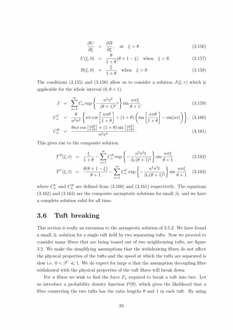
∂U
∂ξ=
∂B
∂ξ, at ξ = θ (3.156)
U(ξ, 0) =θ
1 + θ(θ + 1− ξ) when ξ < θ, (3.157)
B(ξ, 0) =ξ
1 + θwhen ξ > θ. (3.158)
The conditions (3.155) and (3.156) allow us to consider a solution J(ξ, τ) which is
applicable for the whole interval (0, θ + 1).
J =∞∑
n=1
Cn exp
− n2π2
(θ + 1)2τ
sin
nπξ
θ + 1, (3.159)
CUn =
θ
n2π2
nπ cos
[nπθ
1 + θ
]+ (1 + θ)
(sin
[nπθ
1 + θ
]− sin[nπ]
), (3.160)
CBn =
θnπ cos[nπθ1+θ
]+ (1 + θ) sin
[nπθ1+θ
]
n2π2. (3.161)
This gives rise to the composite solution:
TB(ξ, t) =ξ
1 + θ−∞∑
n=1
CBn exp
− n2π2t
βU (θ + 1)2
sin
nπξ
θ + 1(3.162)
TU (ξ, t) =θ(θ + 1− ξ)
θ + 1−∞∑
n=1
CUn exp
− n2π2t
βU (θ + 1)2
sin
nπξ
θ + 1(3.163)
where CUn and CB
n are defined from (3.160) and (3.161) respectively. The equations
(3.162) and (3.163) are the composite asymptotic solutions for small βU and we have
a complete solution valid for all time.
3.6 Tuft breaking
This section is really an extension to the asymptotic solution of 3.5.2. We have found
a small βU solution for a single tuft held by two separating tufts. Now we proceed to
consider many fibres that are being teased out of two neighbouring tufts, see figure
3.2. We make the simplifying assumptions that the withdrawing fibres do not affect
the physical properties of the tufts and the speed at which the tufts are separated is
slow i.e. 0 < βU 1. We do expect for large n that the assumption decoupling fibre
withdrawal with the physical properties of the tuft fibres will break down.
For n fibres we wish to find the force Fn required to break a tuft into two. Let
us introduce a probability density function P (θ), which gives the likelihood that a
fibre connecting the two tufts has the ratio lengths θ and 1 in each tuft. By using
85

symmetry, we can consider θ ∈ [0, 1], which translates to lB ∈ [0, l2], which covers half
the possibilities of fibre ratios in the bottom tuft. Therefore, we require that
∫ 1
0
P (θ′)dθ′ =1
2. (3.164)
Examples of suitable functions that could represent the distribution of n-fibres con-
necting the two tufts are
P (θ) =1
2, (3.165)
P (θ) = 1− θ, (3.166)
P (θ) = θ, (3.167)
see figure 3.2. The first equation (3.165) represents the scenario that for the n fibres
it is equally likely to find any ratio of lengths. The second example (3.166) considers
the case where the lengths of each fibre, which connect the two separating tufts, are
predominantly in one or the other. Finally equation (3.167) could be a simulation of
fibres that are predominantly equally distributed in the two tufts.
0.1 0.2 0.3 0.4 0.5 0.6 0.7
0.25
0.5
0.75
1
1.25
1.5
1.75
2
time
F10
p(θ) = θ
p(θ) = 1− θp(θ) = 1
2
Figure 3.16: The force required to pull two tufts apart held by 10 fibres
To find the force resisting the breaking of a tuft which is being continually elon-
gated, we need to consider the force required to pull these apart. If we consider n
fibres that contribute individually with force F (t; θ), then the expected total force Fn
can be found with the use of the length ratio distribution P (θ):
Fn = 2n
∫ 1
0
P (θ)F (t, θ)dθ, wheneverF > 0. (3.168)
86
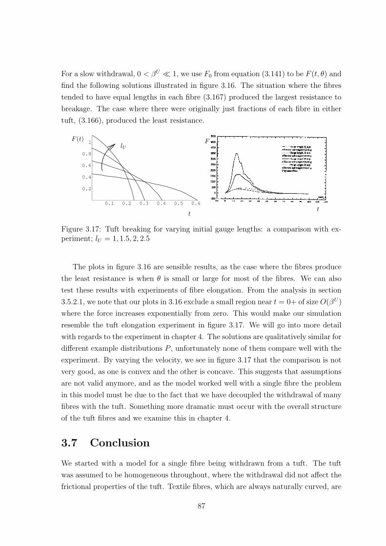
For a slow withdrawal, 0 < βU 1, we use F0 from equation (3.141) to be F (t, θ) and
find the following solutions illustrated in figure 3.16. The situation where the fibres
tended to have equal lengths in each fibre (3.167) produced the largest resistance to
breakage. The case where there were originally just fractions of each fibre in either
tuft, (3.166), produced the least resistance.
0.1 0.2 0.3 0.4 0.5 0.6
0.2
0.4
0.6
0.8
1F (t)
lU
t
F
t
Figure 3.17: Tuft breaking for varying initial gauge lengths: a comparison with ex-periment; lU = 1, 1.5, 2, 2.5
The plots in figure 3.16 are sensible results, as the case where the fibres produce
the least resistance is when θ is small or large for most of the fibres. We can also
test these results with experiments of fibre elongation. From the analysis in section
3.5.2.1, we note that our plots in 3.16 exclude a small region near t = 0+ of size O(βU )
where the force increases exponentially from zero. This would make our simulation
resemble the tuft elongation experiment in figure 3.17. We will go into more detail
with regards to the experiment in chapter 4. The solutions are qualitatively similar for
different example distributions P , unfortunately none of them compare well with the
experiment. By varying the velocity, we see in figure 3.17 that the comparison is not
very good, as one is convex and the other is concave. This suggests that assumptions
are not valid anymore, and as the model worked well with a single fibre the problem
in this model must be due to the fact that we have decoupled the withdrawal of many
fibres with the tuft. Something more dramatic must occur with the overall structure
of the tuft fibres and we examine this in chapter 4.
3.7 Conclusion
We started with a model for a single fibre being withdrawn from a tuft. The tuft
was assumed to be homogeneous throughout, where the withdrawal did not affect the
frictional properties of the tuft. Textile fibres, which are always naturally curved, are
87

approximated by a linearly elastic centre-line. After deriving a model that consisted
of a nonlinear parabolic partial differential equation with a free boundary condition,
we validated the model by testing the solutions against experiment. We then went on
to consider two industrially relevant applications of the simpler single fibre withdrawal
problem. The first scenario was a hook that moved through a tuft and grabbed a
fibre, and the point of interest was whether or not the fibre would be withdrawn
completely or partially. The second scenario went on to consider the case when a
hook or a few hooks grab part of a dense tuft. Then the elongational forces break
the tuft into two, where there are interconnecting fibres. Although we start with just
one interconnecting fibre, we progress to consider many interconnecting fibres. The
results are not completely satisfactory and this leads us on to consider how entangled
fibres are broken down into individuals in the next chapter.
88

Chapter 4
Continuum Models for InteractingFibres
Figure 4.1: A picture of the lap consisting of polyester fibres.
89

4.1 Introduction
We investigate a model for deformations in large populations of inter-connected, ap-
proximately inextensible man-made and natural fibres. In chapter 3, we assumed that
the fibre extraction did not affect the tuft structure. The next step is to focus on how
forces applied to a entangled body of fibres result in the disordered fibre structures
being broken down either into individual fibres or into tufts in which the fibres are
in a more ordered state. Teasing many fibres simultaneously or combing tufts which
cause non-recoverable changes is fundamental to the carding process, and therefore
understanding the transport of fibres relative to one another is crucial if one is to
engage in good carding practice.
Much work on fibre structures consider elastic or visco-elastic deformations in fibre
structures (Buckley, 1980, Pheonix, 1999, Phoenix, 1979). A material composed of
coherent textile fibres will initially respond elastically to stress but our main focus is
on a process that destroys implicit structures that allow for elastic recovery. On the
other hand, visco-elastic models such as those by Maxwell and Jeffreys (Fowler, 1997)
have creeping and relaxation time scales, and are not relevant in the carding machine
as the relaxation time scale is negligible. Therefore we consider a novel approach that
models large populations of inter-connected tufts and fibres under tension, which on
a macroscopic scale will behave as a viscous material.
We begin with a simple approach that considers fibre density and velocity as the
variables in a continuum model. By solving conservation equations for mass and
momentum we find solutions for an elongational flow. After comparing simulations
with experiment we find that except for the initial part of the experiment when
the fibres are re-orientating, the forces in the model were in good agreement with
experiment. Even though the model compares reasonably well with experiment for
the majority of time, we look to include other variables so that we can capture the
behaviour of the re-orientating “alignment phase” and this also allows us to predict
how the internal structure of the lap evolves during the process. The initial “alignment
phase” does not significantly change the density of the tuft or fibre structure, but it
can be thought of as placing the fibres in a state of tension.
We use a vector field to describe average-fibre directionality, and to avoid ambi-
guity in what directionality describes in terms of fibre arrangements, we introduce
an associated scalar field that measures the microscopic alignment to this direction.
In the scientific theories of liquid crystals, there is a particular method to describe
90
the aforementioned directionality and alignment (de Gennes, 1974, Doi and Edwards,
1986, Leslie, 1968) and we gratefully adopt their approach and terminology.
The evolution of each of the new variables requires the introduction of their re-
spective governing equations, and we also need to consider how directionality and
alignment affect the material’s response to stress. There are a number of theories
of mathematics and theoretical physics that attempt to incorporate anisotropies, for
example nematic liquid crystals or fibres in a suspension of fluid. One such example is
the theory of polymers that encompasses a number of interesting modelling concepts,
which may be applicable to a fibrous assembly. A possible modelling assumption
we could employ is polymer reptation, which occurs when a molecular chain in a
concentrated polymer solution is constrained to move strictly in a geometry that is
prescribed by its neighbouring molecules. This may be relevant when extracting a
single fibre but does not apply in the current situation when the whole mass of fibres
is distorted by the applied forces.
Forest et al. (1997) consider how to incorporate directionality and degree of align-
ment into a stress tensor for a polymeric liquid crystal; although the physical prop-
erties of the material may be different there are some fundamental similarities in
design. Closer to the study of fibrous materials are the mathematics applied in fluid
suspensions (Hinch and Leal, 1975, 1976), fibre-reinforced fluids (Spencer, 1972, 1997)
and planar constrained dense fibre arrays (Toll and Manson, 1994, 1995) and using
similar ideology we conjecture a bulk stress tensor. Although there are a number of
analogies with many-body fluid suspensions, there are clearly some major differences
in the physics involved, such as the absence of pressure and advection in a fibre only
continuum. We derive a set of coupled Eulerian field equations, which are composed
of conservation laws, a kinematic condition, and a constitutive evolution equation.
Comparison with experimental data shows that our model with directionality and
alignment to be a good starting point for modelling entangled fibres in the carding
machine. Although the qualitative behaviour is captured in our simulations we find
that there are counter-intuitive problems due to the exclusion of the concept of en-
tanglement. This leads us onto consider inter-fibre topologies within the continuous
medium.
The final piece of the jigsaw is a scalar function that measures the degree of inter-
fibre entanglement. Entanglement is a subject that has seen little coverage in the
scientific press, and we define a method of quantifying the degree of entanglement by
analysing the topology of braids. The description of braids based on group theory is
somewhat sophisticated for our purposes, but it does give a complete methodology
91

that allows us to classify the degree of entanglement of tufts found in the carding
machine. We use equivalence classes of braids and the Artin braid relations, and
this allows us to use a one-to-one mapping to define entanglement as a scalar field.
Incorporating the entanglement into the governing equations results in modifying
the stress tensor and introducing an empirical law for its evolution. The revised
theoretical simulations now compare very well with experiments, both for extensional
and shearing scenarios. We also consider how to include the effects of hooks as they
are dragged through the fibres. Thus we establish a promising continuum model that
describes a many-fibre medium.
4.2 Experiments
Figure 4.2: Graphs of the tuft breaking force experiment for cotton with variableelongation velocities. The initial gauge length is 20 mm.
We have been collaborating with experimentalists at the School of Textile Indus-
tries, University of Leeds. In order to aid the analysis and test the validity of our
models we asked the Leeds group to measure the forces required to pull apart a group
of fibres, loosely labelled as a tuft. They kindly agreed to run two experiments titled
“tuft breaking force” and “tuft shear force”.
92

(a) Cotton
(b) Polyester
(c) Wool
Figure 4.3: Graphs of the tuft breaking force experiment with variable initial tuftlengths: force
weightplotted against extension (mm). Elongation speed of 50 mm/min.
93

For the first of the aforementioned experiments polyester, cotton and short fine
wool tufts were tested on the Instron tensile tester at one of four different gauge
lengths (10, 20 , 30 and 40 mm) depending on tuft size. Care was taken to ensure
that a fibre would not be attached to both clamps holding the tuft in place during the
experiment. The elongational speed is 50 mm/min. The experimentalists considered
the tuft to be broken once the force measured on the tensile tester had reached its
maximum. Working from this definition the magnitude of the force at which tufts
are broken down increase with a decrease in initial tuft length. See figure 4.3 for the
results of this experiment. After further discussion this experiment was also carried
out at four speeds 50, 100, 400 and 500 mm/min, see figure 4.2.
In the second experiment, tuft shear force, a tuft was placed between two wired
surfaces where one traversed the other. The distance between the hooks were varied
(0.007, 0.01 and 0.013 inches), as well as the relative velocity of surfaces (50, 100 and
200 mm/min). On the moving surface a tensile tester measured the forces during the
motion. The shear force experiment in some senses mimics the environment of the
carding machine although in reality the disparity in surface speed is usually between
O(104) and O(105) mm/min. As in the tuft breaking experiment polyester, cotton
and wool fibre tufts were used, see figures B.1, B.2, and B.3 in appendix B.
The consistency of the graphs can be called into question. We highlight two
possible anomalies, one in the tuft breaking force problem with variable speeds, see
figure 4.2, and the other is in the tuft shear force experiment, see B.3 in appendix B.
In the tuft breaking experiment it is difficult to explain why the resistive forces for
elongational speeds 100 mm/min and 400 mm/min are similar and then we observe
a force that approximately doubles when the speed is increased by just 100 mm/min.
For the tuft shear force experiment, there is a dramatic increase in the force and in
the location of the maximum, for speeds of 100 and 200 mm/min, when the distance
between surfaces decrease from 0.01 inches to 0.007. We can also see differences in
the measured forces in the two similar but independent cotton experiments of figures
4.2 and 4.3, which display the measurements for cotton tufts of gauge length 20 mm
elongated at speed 50 mm/min. It is difficult to replicate any experiment involving
tufts that are taken from the lap in a consistent way as the tufts used must differ in
terms of initial entanglement and orientation.
94

4.3 A Simple Viscous Model
There is considerable complexity if one attempts to create a model that incorporates
every single interaction between all fibres in the lap. We have chosen a macroscopic
model in an attempt to get a usable and tractable model. Alternatively we could use
a microscopic approach, whereby probability density functions for microscopic scales
are integrated and averaged to give macroscopic variables. To significantly improve
on a continuum model, we would need to consider discrete interactions but this will
dramatically increase complexity and the mathematics quickly becomes impenetrable.
Furthermore, evolution of many-fibre topologies, see figure 4.7, is difficult to encap-
sulate succinctly consequently making the microscopic method cumbersome. For the
industrialist, the process of disentangling and ordering fibres is only really important
from a macroscopic point of view, as it is the sliver and its intrinsic qualities that
interests the textile manufacturer. So we build a continuum model that encapsulates
the essentials of the carding material without having to account for every single phys-
ical interaction. We begin the modelling process by considering a continuum model
and begin with the simplest case first.
We define the Eulerian scalar function ρ(x, t) to be the average fibre density or
volume fraction,
ρ =NV πa
2l
V, (4.1)
where NV is the number of fibres in volume V , a and l are average fibre radius
and length respectively. The vector function u(x, t) is the average velocity of the
fibres. We make the rather crude assumption that the global behaviour of the micro-
structure, consisting of many interacting fibres, is that of an isotropic medium. The
two factors that give rise to internal forces and structural rigidity are individual
contact points between fibres and the orientation of the fibre network. We neglect
aerodynamic forces, electro-static forces and gravity. These assumptions are tested
by juxtaposing simulation with experiment.
4.3.1 Problem Formulation
Using conservation laws for mass and momentum (Batchelor, 1967) we write down
the governing field equations, in an arbitrary domain V , for a tuft population:
∂ρ
∂t+ ρ
∂uk∂xk
+ ul∂ρ
∂xl= 0, (4.2)
ρ
(∂ui∂t
+ uk∂ui∂xk
)=
∂σil∂xl
+ fi, (4.3)
95

where we employ the summation convention, σij is the stress tensor and fi are the ex-
ternal body forces. It is necessary to impose an initial state, and boundary conditions
at ∂V , if we wish to find a solution and an example of these are:
u(x, t) = u0(x)ρ(x, t) = ρ0(x)
at t = 0 with u(x, t) or σijnj given on ∂V, (4.4)
where x = (x1, x2, x3)T and u = (u1, u2, u3)T . To close the system of equations
(4.2) and (4.3) it remains to relate stress with velocity, or rate-of-strain, using a
constitutive assumption. The simplest approach is to use a Newtonian viscous stress
tensor (Batchelor, 1967), which suggests that stress is linearly proportional to the
rate-of-strain:
σij =µ
2
(∂ui∂xj
+∂uj∂xi
)+ λ
∂uk∂xk
δij (4.5)
where δij is the Kronecker delta and µ and λ are effective viscosities which will depend
on frictional forces generated by fibre-fibre contact points.
4.3.1.1 Fibre Contact Points
To complete the equations we would like to incorporate the effect of friction between
fibres. We can now explore the relationship between the viscous coefficient µ in
equation (4.5) and space x, velocity u and density ρ. By considering two extreme
situations we can gain some idea of how we can implement this into our model. When
we take the limit as fibre density tends to zero we expect µ, λ → 0 and conversely
when the density of fibres tends to unity we postulate that µ, λ→∞. Assuming that
a greater density implies a greater number of contact points per unit volume, then
one would expect the viscous coefficient µ to depend on density (4.1). We could use a
number of power laws based on intuition, but we can refine this assumption by using
a probabilistic method based on the work of Komori and Makishima (1977).
Let us define a region bounded by parallel planes that intersect the centre lines
of two straight fibres A and B; the fibres have polar angles (θ, φ) and (θ′, φ′), and
their respective surfaces are in contact at one point. By connecting the corresponding
vertices with straight line segments, we have a parallelepiped, the bases have lengths
l, the average length of a fibre, see figure 4.4. The volume of the parallelepiped is
v1(θ, φ; θ′, φ) = 2al2 sinχ, (4.6)
where χ is the angle between two adjacent sides of the base or equivalently the angle
between the axes of the fibres A and B, see figure 4.4, and this is explicitly:
cosχ = cos θ cos θ′ + sin θ sin θ′ cos(φ− φ′). (4.7)
96

l
(θ, φ)
(θ′, φ′)B
χ
l
A
2a
Figure 4.4: A diagram illustrating the likelihood of contact between a couple of fibres.
Whenever the centre of mass of a straight fibre with orientation (θ′, φ′) can be found
in the parallelepiped described in figure 4.4 it will necessarily make contact with
fibre A. Equally this would also be true if we reflected the volume through the
plane intersecting A; this means that we are concerned with a larger parallelepiped
of depth 4a, centred on A and this volume is labelled as v = 2v1. We assume that the
distribution of the centre of mass, of B, is random throughout the material concerned,
and we also neglect the frictional forces due to the fibre ends, which is acceptable for
fibres with small aspect ratio al 1. The probability that a fibre B comes into
contact with A is equivalent to the probability that the centre of mass of B can be
found in the volume v:
P (C ⊂ V ) = P (θ, φ; θ′, φ′) =v
V=
4al2
Vsinχ, (4.8)
where V is an arbitrary volume that contains v. When N fibres are in V in addition
to fibre A, the average number of of fibre contact points or crossings on A is
n(θ, φ) = N
∫ π
0
∫ π
0
P (θ, φ; θ′, φ′)Ω(θ′, φ′) sin θ′dθ′dφ′ (4.9)
=4al2N
V
∫ π
0
∫ π
0
Ω(θ′, φ′) sinχ sin θ′dθ′dφ′, (4.10)
where Ω is defined such that the probability of finding a fibre with orientation (θ +
∆θ, φ+ ∆φ) as ∆θ and ∆φ→ 0 is Ω(θ, φ) sin θdθdφ. The average number of contact
points for an arbitrary fibre of length l is
n =4aNl2
VI (4.11)
97
where
I =
∫ π
0
∫ π
0
∫ π
0
∫ π
0
Ω(θ′, φ′)Ω(θ, φ) sinχ sin θdθ′dφ′dθdφ. (4.12)
As we have not incorporated a quantity that represents directionality or alignment in
this model then I in equation (4.12) is constant. We do, however, go on to introduce
such variables and these will be closely related to I. This means that by considering
the average length of fibre in a unit volume we can predict the number of contact
points per volume V , and this can be written in terms of the density as follows:
ν =2aN 2l2I
V=
2I
π2a3ρ2. (4.13)
This result that ν is proportional to ρ2 coincides with work by Toll (1993) and Toll
and Manson (1994) and can also be generalised for non straight fibres (Komori and
Makishima, 1977). We could evaluate I in a number of orientations, for example
either totally random Ω(θ, φ) = 12π
or aligned Ω(0, 0) = δ(θ)δ(φ). Therefore we begin
by modelling the viscous coefficient in (4.5) by:
µ = ν1ρ2 and λ = ν2ρ
2, (4.14)
where ν1 and ν2 are constant. We note that for highly heterogeneous densities, the im-
plicit assumption that the centre of masses of fibres in V being uniformly distributed
is no longer valid, but for our purposes this assumption is adequate. Now the model
is complete, though parameters ν1 and ν2 are still unknown.
The governing equations (4.2) - (4.3) represent a continuum of fibres and to verify
the modelling assumptions made in this section we test theoretical experiment with
reality. The simplest case for both experiment and mathematical solution leads us to
consider the quasi one-dimensional problem of a tuft or entangled fibre-mass being
elongated.
4.3.2 Dimensionless Equations
Before we go on to solve the problem (4.2), (4.3), (4.5) and (4.14), in order to give
greater understanding into the interplay between their respective terms we find their
dimensionless form. The velocity is scaled with a representative value of u(x0, t) from
the boundary conditions (4.4), U, and similarly for the density a suitable quantity
from ρ0(x) or ρ(x0, t), which we call ρ. Scaling distance with the length-scale l, the
98

initial size of the tuft, and time with lU
means the equations (4.2), (4.3), (4.5) and
(4.14) can be re-written as
∂ρ
∂t+ ρ
∂uk∂xk
+ ul∂ρ
∂xl= 0, (4.15)
ρ
(∂ui∂t
+ uk∂ui∂xk
)= Λ
∂σil∂xl
, (4.16)
where
σij = ρ2
(eij +
ν2
ν1
∂uk∂xk
δij
), (4.17)
eij =1
2
(∂ui∂xj
+∂uj∂xi
), (4.18)
eij is the linear rate-of-strain tensor in dimensionless form and we have assumed
that there are no external body forces fi = 0. The dimensionless scalar Λ = ν1ρUl
is
analogous to the inverse of the Reynolds number.
To find an estimate for the size of the parameter Λ, we use the experimental data
given in section 4.2, in figure 4.3. The load for cotton, with initial gauge length of 10
mm, is 132.4 grams for the point at which the extensional force is at its maximum,
and the corresponding force of 1.29752 Newtons, see figure 4.3 and appendix B. When
we compare this to the force generated by the fibre contact points in unidirectional
extension, approximated by F = ν1ρ2 ∂u∂x∼ ν1ρ
2Ul
where density, velocity and length
scale with ρ ∼ 102kgm−3, U ∼ 10−3ms−1, and length l ∼ 10−3m respectively, then
ν1 ∼ 10−2 with dimensions m3kg−1s−1. This means that Λ is O(105) for the exper-
iment and in the carding machine itself, basing the length on the distance between
cylinder surfaces O(10−2) m/s and typical velocity as O(1) m/s, is O(102). Therefore
we shall consider Λ to be large, and this means that the viscous terms dominate over
the inertia terms in equation (4.16).
It must be noted that we never expect a scenario for the motion of entangled
fibres to display noticeable inertia, due to the internal forces generated by fibre-fibre
contact points. For the textile fibres concerned, a low density fibrous media could be
modelled as hydro-dynamically dilute or semi-dilute suspension, and the model may
include inertia but it would then be driven by the fluid dynamics.
4.3.3 The Extensional Simulation
A group of entangled fibres, that form a tuft, can be represented by a simply connected
region in a field. The tuft, unlike a fluid, will retain its initial structural integrity
99

when ambient body forces are applied, such as gravity. Our microscopic structures
that form the continuum are on the scale of microns, unlike conventional fluid flows
that are fundamentally based on molecular interactions. We shall neglect any effects
due to the tuft boundaries, such as surface tension due to the lack of any meniscus
forces. Alternatively one could view this as the tuft being of infinite in width. A tuft
Fixed Clamp Moving Clamp Moving ClampFixed Clamp
Figure 4.5: A diagram of unidirectional elongation.
of length l(t) is pulled apart with force F (t) and speed U(t), see figure 4.5, where
either the force or the rate of extension may be specified on one boundary and the
other boundary is held fixed.
For the experiments the elongation speed U(t) = U0 is constant throughout and
the tuft length varies but has initial length l. We treat the body as quasi one-
dimensional and work with one spatial dimension x and time t, which means that
u = u(x, t)i and ρ = ρ(x, t). For the governing field equations we explicitly specify
the scalings for the dimensionless form: distance with l, viz. x = lx′, velocity U with
U0 and density ρ with the maximum initial density ρ(x, t = 0). Equations (4.15) –
(4.17) with Λ 1, become
∂ρ
∂t+
∂
∂x(ρu) = 0, (4.19)
∂
∂x
(ρ2∂u
∂x
)= 0. (4.20)
With the aforementioned scalings, the moving boundary has speed unity, and the
initial and boundary conditions become
ρ = ρ0(x) at t = 0, and u = 0 at x = 0, (4.21)
ρ2∂u
∂x= F (t) and u = 1 at x = 1 + t. (4.22)
The form of (4.19) suggests that a Lagrangian formulation would be appropriate if we
wish to find analytical solutions. By letting ξ represent a particular material element
100

throughout the motion, position is now a function of element and time, x = X(ξ, t).
Velocity is therefore defined as ∂X(ξ,t)∂t
∣∣∣ξ
= u(x, t). Then X = 1 + t at ξ = 1, which
is the point of the fibre continuum that is dragged away by the moving boundary.
Under the transformation of variables we find that the Lagrangian formulation of the
field equations (4.19) – (4.20) become:
∂ρ
∂t+ ρ
∂u
∂ξ
∂ξ
∂x= 0, (4.23)
∂ξ
∂x
∂
∂ξ
(ρ2∂u
∂ξ
∂ξ
∂x
)= 0. (4.24)
The boundary conditions (4.21) and (4.22) are now:
ρ = ρ0(ξ) at t = 0, and u = 0 at ξ = 0, (4.25)
σ11 = F (t) and u = 1 at ξ = 1, (4.26)
where ξ[X(ξ, t), t] = ξ and ∂ξ∂x
∂x∂ξ
= 1. Substituting (4.23) and also using the first
equation in (4.26), equation (4.24) becomes:
−ρ(ξ, t)∂ρ(ξ, t)
∂t= F (t). (4.27)
A parametric solution can be found by integrating equation (4.27), and imposing the
initial condition in (4.25) the solution is:
ρ(ξ, t) =
√ρ0(ξ)2 − 2
∫ t
0
F (s) ds, X(ξ, t) =
∫ ξ
0
ρ0(p)dp√ρ0(p)2 − 2
∫ t0F (s) ds
. (4.28)
Applying the boundary condition at ξ = 1 so that X(1, t) = 1 + t gives the force at
the moving clamp, F (t) from (4.28). The case when we have a uniform initial density,
ρ0(ξ) = 1 is particularly straightforward to solve, and in this case:
u = ξ, F (t) =1
(1 + t)3and ρ(t) =
1
1 + t. (4.29)
This gives monotonic decreasing functions in time for both the withdrawal force and
the density, which is similar to the analogous hydrodynamic simulation.
The dimensional force from (4.29) is Fdim(t) =ν1Uρ2
0l2
(l+Ut)3 . This agrees well with the
experiment but only when the tuft breaking force has reached its maximum, see figure
4.6. If we visualise the experiment, the fibres orientate themselves to the direction of
extension in the initial stage and then are pulled apart in the latter stage. We have
assumed that the fibre structures have not fractured, but even if they don’t fracture,
as ρ→ 0 the continuum assumption will break down.
101
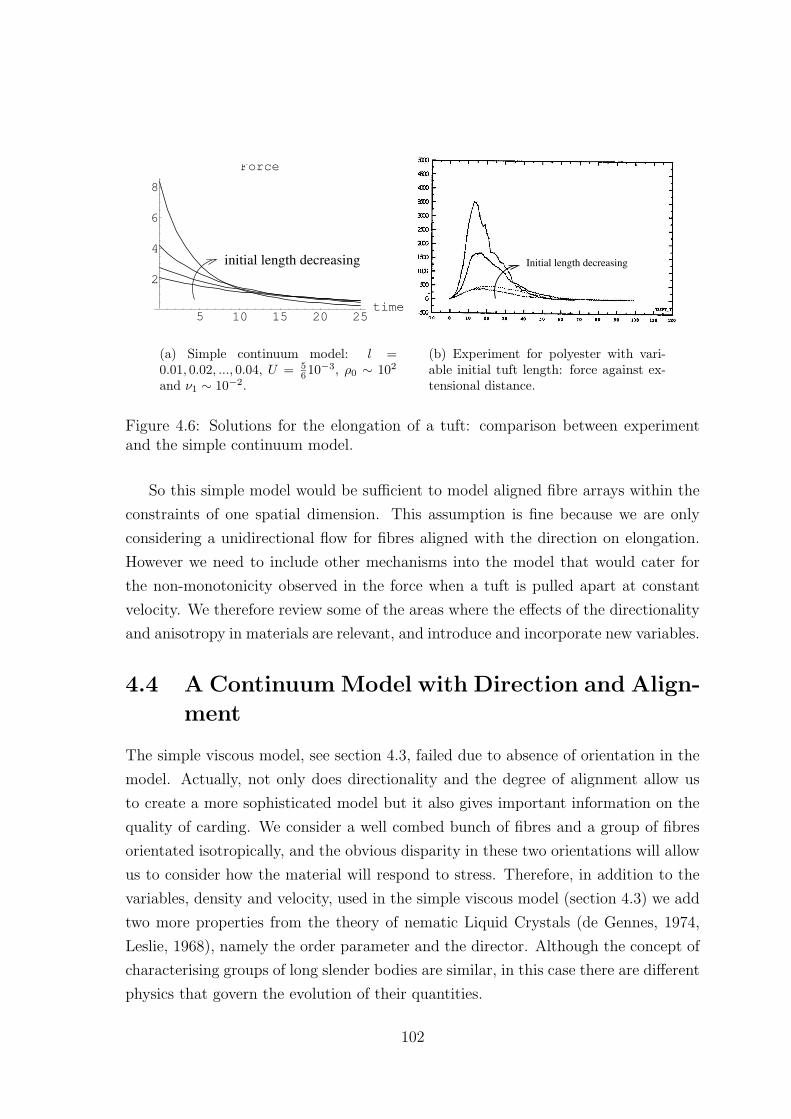
5 10 15 20 25time
2
4
6
8
Force
initial length decreasing
(a) Simple continuum model: l =0.01, 0.02, ..., 0.04, U = 5
610−3, ρ0 ∼ 102
and ν1 ∼ 10−2.
Initial length decreasing
(b) Experiment for polyester with vari-able initial tuft length: force against ex-tensional distance.
Figure 4.6: Solutions for the elongation of a tuft: comparison between experimentand the simple continuum model.
So this simple model would be sufficient to model aligned fibre arrays within the
constraints of one spatial dimension. This assumption is fine because we are only
considering a unidirectional flow for fibres aligned with the direction on elongation.
However we need to include other mechanisms into the model that would cater for
the non-monotonicity observed in the force when a tuft is pulled apart at constant
velocity. We therefore review some of the areas where the effects of the directionality
and anisotropy in materials are relevant, and introduce and incorporate new variables.
4.4 A Continuum Model with Direction and Align-
ment
The simple viscous model, see section 4.3, failed due to absence of orientation in the
model. Actually, not only does directionality and the degree of alignment allow us
to create a more sophisticated model but it also gives important information on the
quality of carding. We consider a well combed bunch of fibres and a group of fibres
orientated isotropically, and the obvious disparity in these two orientations will allow
us to consider how the material will respond to stress. Therefore, in addition to the
variables, density and velocity, used in the simple viscous model (section 4.3) we add
two more properties from the theory of nematic Liquid Crystals (de Gennes, 1974,
Leslie, 1968), namely the order parameter and the director. Although the concept of
characterising groups of long slender bodies are similar, in this case there are different
physics that govern the evolution of their quantities.
102

Figure 4.7: A plan view of the fibre arrangement as they enter the carding machine.
The director a, is a unit vector and φ is the associated order. The director
represents the macroscopic-average direction of the fibres local to a given point. A
group of fibres that have the same average direction can vary in terms of the degree
to which the individual fibres are aligned to the average direction. In figure 4.8, we
see that a 3-fibre bundle can have the same director but the orientation is different,
and so this ambiguity is eliminated by using an order parameter φ.
At each point we measure the fibre orientation with a given directionality. If a
typical fibre-tangent lies at an angle θ relative to a given unit vector a, see figure 4.9,
the order parameter is related to the average angle θ between all the neighbouring
fibres and the director, more specifically
φ = E
[3 cos2 θ − 1
2
]. (4.30)
where E is the average over all fibres in a neighbouring region. For any arbitrary unit
vector a, we can specify an order parameter for a given group of neighbouring fibres.
So we specify a unique macroscopic directionality a to be the unit vector for which
the order φ attains its maximum value. The limits of the order parameter suggest
three distinct states: “nematic” φ = 1, “isotropic” φ = 0 and “planar” φ = − 12.
An illustration of these are given in figure 4.10. The “planar” case, in figure 4.10,
which is a viable form in liquid crystals but is physically unlikely in our fibre model,
particularly when the material is dilated, sheared or elongated. Therefore, we could
assume that the order parameter will always lie between the isotropic to random
phases inclusively, i.e. φ ∈ [0, 1]. Furthermore in this chapter we shall only consider
two dimensional cases, which make the planar isotropy φ = − 12
redundant. We note
103

fibre tangents
a a
fibre tangents
Figure 4.8: A comparison of a couple of 3-fibre bundles with the same average direc-tionality.
θ
Fibre
Fibre Tangent
unit vector
Figure 4.9: An illustration of the angle averaged for the order parameter.
that φ is closely related to I defined in 4.12, but it is different because the the average
direction a is implicit in the definition of φ, whereas I measures the general degree
of alignment.
4.4.1 The Governing Equations
At the moment, to describe the fibre medium, we have an order parameter φ, a
director a, density ρ and components of velocity ui. Conservation laws for mass
and momentum (4.2) and (4.3) respectively are given in the simple viscous model of
section 4.3 and these are still valid in this more sophisticated model.
For the “simple viscous” model in section 4.3 we neglected inertia by assuming
104

!!!!!!!!!!!!!!!!!!!!!!!!!!!!!!!!!!!!!!!!!!!!!!!!!!!!!!!!!!!!!!!!
""""""""""""""""""""""""""""""""""""""""""""""""""""""""""""""""
#$#$#$##$#$#$##$#$#$##$#$#$##$#$#$##$#$#$##$#$#$##$#$#$##$#$#$#
%$%$%$%%$%$%$%%$%$%$%%$%$%$%%$%$%$%%$%$%$%%$%$%$%%$%$%$%%$%$%$%
&$&&$&&$&&$&&$&&$&&$&&$&&$&
'$''$''$''$''$''$''$''$''$'
((((((((((((((((((((((((((((((((((((((((((((((((((
))))))))))))))))))))))))))))))))))))))))))))))))))
****************++++++++++++++++
,$,$,,$,$,,$,$,,$,$,,$,$,,$,$,,$,$,,$,$,,$,$,
-$--$--$--$--$--$--$--$--$-
.$.$.$..$.$.$..$.$.$..$.$.$..$.$.$..$.$.$..$.$.$..$.$.$.
/$/$/$//$/$/$//$/$/$//$/$/$//$/$/$//$/$/$//$/$/$//$/$/$/
"nematic""planar"
"isotropic"
Figure 4.10: Three distinct states for liquid crystals that can be represented by theorder parameter: φ = − 1
2, φ = 0 and φ = 1 respectively.
that Λ 1 and this assumption, that the frictional forces induced by the contact
points dominate over the advective properties of the material, is still valid. So with
negligible inertia, conservation of momentum (4.3) becomes
∂σik∂xk
+ fi = 0, (4.31)
where fi are the components of the external body forces and σij is the stress tensor.
However we need to incorporate the effects of the new characteristic quantities, di-
rectionality and degree of alignment, into the stress-rate-of-strain relationship, and
this forms a key component in our model.
4.4.1.1 The Stress Tensor
Much of the work on fibres in fluids produce a bulk stress tensor that includes a
component from the fluid and a component from the fibre interactions. Usually the
fluids concerned are treated as Newtonian (Batchelor, 1971, Hinch and Leal, 1976,
Spencer, 1972, Toll and Manson, 1995) where the bulk stress tensor varies depending
on the physical effects of the fibres concerned. Hinch and Leal (1975, 1976) derive
governing equations for a material where “micro-scale” interactions are averaged into
a “macro-scale” continuous media. The authors focus on particles in a Newtonian
fluid suspension described by a single scalar-type function and a direction-function,
which are similar to our order parameter and director. A volume average of the
micro-structural state described by a probability density function N governed by the
Fokker-Planck diffusion equations is related to the bulk stress consisting of a normal
viscous component and a contribution due to the fibres,
σij = −pδij + 2µeij + 2µΦ 2A〈aiajakal〉ekl+
105

2B [〈aiakejk + ajakeki〉] + Ceij + F 〈aiaj〉D . (4.32)
〈·〉 denotes the average with respect to the the probability density function N and
A,B,C, and F are shape factors, Φ is a small volume fraction of fibres and µ the
Newtonian viscosity. The terms multiplied by the volume fraction in equation (4.32),
with the exception of the last term which is multiplied by the shape factor F , are
the same as the stress tensor for an incompressible viscous, transversely isotropic
medium. We go on to look at transverse isotropy when we derive our stress tensor
and illustrate this point more clearly.
Toll and Manson (1994, 1995) are the only authors that focus on viscous defor-
mations in fibre suspensions where the fibre-fibre contact points make a significant
contribution to the bulk stress, although there are numerous articles that study elastic
and visco-elastic deformations such as (Pheonix, 1999, Phoenix, 1979) and (Buckley,
1980) respectively. An analytical form of stress is found where linear friction domi-
nates over hydrodynamic effects and the cases of nearly random orientation, shearing
and extensional flows are given. This work is the closest study to that of the card-
ing machine, but the body of fibres we are interested in do not have any internal or
external forces keeping an array of fibres approximately planar. Axial fibre rotations
under planar compression form the distinctive part of this model.
Spencer (1972) examines fibre-reinforced materials. Similar to the work by Hinch
and Leal (1975, 1976) the stress tensor has two components, a reaction stress due to
the constraints and a remainder stress which is dependent on the chosen material. In
general, dynamic cases involve a reaction stress that is dependent on strain-rates and
for elastic fibres a remainder stress that is proportional to strain. None of the cases
studied focussed on the effect of interacting particles which play an important role in
the carding process, but we do adopt a similar ethos in creating our model, with bulk
stress consisting of isotropic and anisotropic components and the use of transverse
isotropic symmetries in our continuum model.
The stress tensor for an anisotropic material needs special consideration. We write
the bulk stress tensor as two components, and these are derived from considering the
two distinct fibre orientations, random and nematic. If the material is in the nematic
phase, see figure 4.11, where all the fibres are theoretically aligned, we expect a line
of symmetry about the direction of alignment, and the stress tensor should also be
independent of a reflection through a plane transverse to this line. This physical
phenomena is called transverse isotropy and it is well documented for linear elasticity
(Green and Zerna, 1968, Love, 1927, Spencer, 1972). When the fibres are randomly
106

σxx
σxy σxy
σyyσyy
Nematic Random
σyxσyx
σxx
Figure 4.11: A diagram of the stresses acting on a nematic body of fibres and arandomly orientated body of fibres.
arranged, the medium will respond as an isotropic medium, and this has already been
described in section 4.3.
To derive a transversely-isotropic stress tensor σN , with axial symmetry about a,
we begin by using a similar methodology illustrated in Love (1927) where the director
is treated as constant, a = (0, 0, 1)T , but for a viscous material, which assumes that
stresses are related linearly to strain-rates. The stress tensor is then generalised for
an arbitrary directionality.
By representing stress and strain rates with six-vectors, three components for
dilation and three for torsion, we can write:
σ =
σxxσyyσzzσyzσzxσxy
= C
uxvywz
vz + wywx + uzuy + vx
(4.33)
where C is a square symmetric six by six matrix. To deduce the form of C we need
to ensure that the strain-rate energy function W , which has the form
2W = c11e2xx + c12exxeyy + c13exxezz + c14exxeyz + c15exxezx + c16exxexy
+c22e2yy + c23eyyezz + c24eyyeyz + c25eyyezx + c26eyyexy
+c33e2zz + c34ezzeyz + c35ezzezx + c36ezzexy
+c44e2yz + c45eyzezx + c46eyzexy
107

+c55e2zx + c56ezxexy
+ c66e2xy, (4.34)
remains unchanged under rotations within and reflections through the transverse
plane perpendicular to a = (0, 0, 1)T . In (4.34), eij is the rate-of-strain tensor given
in (4.18) and cij are components of the matrix C. The reflection through the plane
perpendicular to a takes the form
x′ = x; y′ = y and z′ = −z. (4.35)
This will leave the energy function (4.34) unchanged only if
c14 = c15 = c24 = c25 = c34 = c35 = c46 = c56 = 0. (4.36)
Similarly if we rotate about z by an angle ψ then we write
x′ = x cosψ + y sinψ; y′ = −x sinψ + y cosψ; z′ = z. (4.37)
By using the chain rule one can write the new rate-of-strain terms:
ex′x′ = exx cos2 ψ + eyy sin2 ψ + exy sinψ cosψ, (4.38)
ey′y′ = exx sin2 ψ + eyy cos2 ψ − exy sinψ cosψ, (4.39)
ez′z′ = ezz, (4.40)
ey′z′ = eyz cosψ − ezx sinψ, (4.41)
ez′x′ = ezx cosψ + eyz sinψ, (4.42)
ex′y′ = exy(cos2 ψ − sin2 ψ)− 2 cosψ sinψ(exx − eyy). (4.43)
The equations (4.38) – (4.43) can be used to express the old strain-rates in vector
form, e, in terms of the new strain-rates e′ = Ree, where Re is a six by six matrix.
Similarly, the rotation also means that the stress vector σ can be related linearly with
the new variable, σ′ = Rsσ, where Rs is a six by six matrix. After the rotation we
expect σ′ = Ce′ as it would be inconsistent if the coefficients in C changed, therefore
we find that
C′ = R−1s CRe. (4.44)
This gives six dependent equations for c11, c12, c13, c16, c22, c23, c26, c36, c44, c45, c55 and
c66. Further algebraic manipulations give the following simplifications:
c11 = c22, c66 =c11 − c12
2, c13 = c23, c44 = c55 and c33 6= 0 (4.45)
c14 = c15 = c16 = c24 = c25 = c26 = c34 = c35 = c36 = c45 = c46 = c56 = 0. (4.46)
108

An alternative to this method has been given by Spencer (1972), which again
considers an elastic medium, but uses linear algebra, namely the Cayley-Hamilton
Theorem. Both methods produce the same result, that is five non-zero coefficients,
in a relatively sparse block-diagonal matrix:
C =
A A− 2N 2F 0 0 0A− 2N A 2F 0 0 0
2F 2F C 0 0 00 0 0 L 0 00 0 0 0 L 00 0 0 0 0 N
, (4.47)
where c11 = A, c13 = 2F , c33 = C, c44 = L, and c66 = N .
We need to generalise this for any director a, and do this using a tensor method.
The stress vector σ and strain-rate vector e can be re-written using tensor notation
σij and eij respectively and the relating coefficients found in C from (4.47) can now
be found in a fourth order tensor Bijrs, and this is written as
σij = Bijrsers. (4.48)
As both stress and rate-of-strain are symmetric, and this imposes the conditions,
Bijrs = Bjirs = Bijsr = Bjisr. (4.49)
For transverse isotropy, most of the elements of the four-tensor, Bijrs, are zero but the
non-zero elements equate to the non-zeros in the matrix equation (4.47) as follows:
B1111 = A2, B1122 = A−2N
2, B1133 = F,
B2211 = A−2N2
, B2222 = A2, B2233 = F,
B3311 = F, B3322 = F, B3333 = C2,
B1212 = N, B1313 = L, B2323 = L.
(4.50)
With a little foresight we rearrange the constants as follows
B2211 = B1122 = λ2
2, B1212 = λ1,
B3311 = B3322 = B1133 = B2233 = λ2
2+ λ4, B1313 = B2323 = λ1 + λ3,
B3333 = λ1 + λ2
2+ 2λ3 + 2λ4 + λ5, B1111 = B2222 = λ1 + λ2
2
(4.51)
and so this gives the form
Bijrs = λ1δirδjs + δisδjr
2+ λ2
δijδrs2
+λ3(δj3δr3δis + δi3δs3δjr + δi3δr3δjs + δj3δs3δir)
2+λ4(δi3δj3δrs + δijδr3δs3) + λ5δi3δj3δr3δs3. (4.52)
109

So far our analysis is valid when a = (0, 0, 1)T , and now we proceed to find the formula
for a general transverse isotropic media with director a = (a1, a2, a3). We rotate the
specified director (0, 0, 1) with an orthonormal matrix tij so ai = tij(0, 0, 1) = ti3,
then
σ′αβ = tαitβjtkrtlsBijrse′kl. (4.53)
Now for the third term in (4.52) we find that
tαitβjtkrtls(δj3δr3δis + δi3δs3δjr + δi3δr3δjs + δj3δs3δir)
= akaβδαl + aαalδβk + aαakδβl + aβalδkl, (4.54)
for the fourth term
tαitβjtkrtls(δi3δj3δrs + δijδr3δs3) = aαaβδkl + akalδαβ, (4.55)
and the final term becomes
tαitβjtkrtlsδi3δj3δr3δs3 = aαaβakal. (4.56)
Thence dropping dashes we find the stress tensor for a general transversely isotropic
material
σNαβ = λ1eαβ + λ2ekk2δαβ + λ3(aαaieβi + aβaieiα)
λ4(aαaβekk + δαβakalekl) + λ5aαaβakalekl, (4.57)
where we have renamed the stress σ which has transverse isotropic symmetries as σNij .
If the material is completely aligned, as in the “nematic phase” in figure 4.11, the
stress tensor should have the form given in (4.57). Notice that if we were to solve
the elongational simulation in section 4.3.3 with the stress tensor (4.57) instead of
equation (4.5), for a = (1, 0, 0)T , the results would be very similar.
The other distinct orientation of the fibre material is the random phase φ ∼ 0,
and we expect a different response such as that of an isotropic medium.
σIαβ = µ1eαβ + µ2ekkδαβ, (4.58)
and this is the same as (4.5).
Adopting a similar approach to Hinch and Leal (1975, 1976) and Spencer (1972),
we break down the stress into two components, which we label nematic and isotropic.
The bulk stress should behave like (4.57) when φ → 1 and when the material is in
110

the random phase φ = 0 we expect (4.58) to dominate. A general form for bulk stress
can be written as
σ = f(φ)σNij + g(φ)σIij , (4.59)
where g and f can take a number of forms. A simple definition that reflects the
difference between the cases φ = 1 and φ = 0 is
g(φ) = (1− φ)m and f(φ) = φn. (4.60)
We will begin with the simplest case first and use a linear relation, m = n = 1.
Finally we need to approximate how the viscous coefficients are dependent on the
frictional contact points. As in the case for the simple viscous model of section 4.3 we
assume that the coefficients are dependent on the square of density. We write each
coefficient as follows:
µi = ρpµi and λi = ρqλi, (4.61)
where p and q are positive constants, and again for simplicity we start our analysis
with p = q = 2.
The stress tensor for a dilute fibre suspension will have the form (4.32) whereas
our fibre continuum has the form (4.59). There are bound to be differences as the
presence of the fluid is significant, where one would expect to include pressure which
is due to the fluid. Spencer (1997) and Hinch and Leal (1975, 1976) both incorporate
pressure into the representative bulk stress. In our stress tensor, unlike (4.32), u is
the velocity of the fibres not the fluid. Although our fibres are surrounded by air
we assume that the aerodynamic contribution to the stress tensor is negligible, our
stress is dominated by fibre-fibre interactions. There are two other differences in the
stress given in (4.59) and (4.32), and they arise from the fluid velocity field being
incompressible whereas our fibrous material is compressible and the fibrous viscous
coefficients being dependent on the number of contact points.
Now we have completed the conservation of momentum equation by defining the
stress (4.59) with viscous coefficients defined by (4.60) and (4.61). We are left with
the task of finding evolution equations for the director and order. These equations
are found in the form of a kinematic condition and an empirical law.
111

x
x+ sa
A
B
x+ u(x)δt
sa
A’
x+ sa+ u(x+ sa)δt
B’
s′a′
Figure 4.12: A diagram illustrating the evolution of the director using kinematics.
4.4.2 Kinematic Condition
The motion of the fibres will govern the evolution of their directionality, and therefore
we derive a governing equation for the director a. Consider an arbitrary element
evolving in time where A → A’ and B → B’, illustrated in figure 4.12, where δt is a
small time and s is a small length scale along a. Applying elementary kinematics we
have the following equation,
s′a′ = sa+ s δt(a · ∇)u+O(s2). (4.62)
Now we take the limit as δt→ 0 and ignoring O(s) terms, we find
∂a
∂t+ (u · ∇)a+
s
sa = (a · ∇)u. (4.63)
where ˙ is full derivative with respect to time. In equation (4.62), we have introduced
a new variable s which represents the length of the element in direction a, and ss
which
represents the rate of extension of a material element. The concept of extensible fibres
and the inclusion of compressibility make this model unique amongst those that model
viscous deformations in fibre suspensions. In the model of fibre reinforced fluids by
Spencer (1972), the fibres are treated as inextensible, and they could represent say
hairs moving in the wind. Our many-fibres’ extensibility will be represented by the
director a and length s, and when the fibres are moved by a non-uniform velocity
field they may be susceptible to viscous deformations, where fibres slide over one
another. This, then, is the crux of our model: fibres slipping over one another.
As the macroscopic continuous medium represents the average of many fibres, this
produces the effect that the macroscopic material elements are extensible. The actual
112
director can be represented by a unit vector
akak = 1, (4.64)
as s takes care of the vector length and s its respective evolution. Consequently we
can eliminate the new variables s if we so desire by using (4.64).
We can contrast the kinematic condition (4.63) with a director for a dilute fibre-
fluid suspension that is driven by the fluid flow (Hinch and Leal, 1975, 1976). When
placed in a time-dependent linear flow u(x, t) = Γ(t)·x with Γ = E+Ω, E = ET and
Ω = −ΩT , symmetric and anti-symmetric tensors, a particle aligned in the direction
of the unit vector a rotates according to
a = Ω · a+G [E · a− a (a ·E · a)] . (4.65)
G represents a shape factor modulus. This means that the evolution of the fibres are
driven purely by the external fluid flow, whereas our director evolves according to the
average fibre velocity (4.63).
4.4.3 Empirical Law for the Order Parameter
Finally we need to find one more evolution equation for the order parameter to close
the system given by (4.2), (4.31), (4.59), (4.60), (4.61), (4.63) and (4.64). There are
a number of scenarios that are possible but we will focus on the effect of density
reducing, elongational and extensional flows. We attempt to encapsulate the leading
order behaviour to get a usable equation, which is based on simple empirical evidence.
If one strains a bunch of entangled fibres, we can see two phases of interaction:
the first involves the orientation of fibres in the direction of the applied force and in
the second phase the fibres begin to slip over one another. This observation cannot be
made categorically for all fibre types and length, nor do we claim that the two phases
are distinct and exclusive processes, but just the dominant qualitative behaviour. So
we conjecture the evolution of the order parameter to be a function of the rate of
extension of the material element ss, and to begin with we use a linear relationship.
Constraining the order parameter to be between zero and unity, where for extensional
or shearing flows we expect φ to be monotonic increasing, we postulate:
∂φ
∂t+ (u · ∇)φ = β(1− φ)
1
s
[∂s
∂t+ (u · ∇)s
], (4.66)
where β is the rate at which the order increases compared to the rate of extension, ss.
We could have used other polynomial functions of φ on the right hand side of equation
113

4.66, but we found when comparing the experimental results of section 4.2 with other
polynomials, 1 − φ is a good starting point. We re-write (4.66) by eliminating s by
using (4.63) with (4.64)
∂φ
∂t+ uk
∂φ
∂xk= β(1− φ)akal
∂uk∂xl
. (4.67)
U ψ
F
Figure 4.13: A diagram that illustrates the evolution of the order parameter with alinearly damped rod.
To support the conjectured evolution equation (4.66), we consider a simple case
of a string, see figure 4.13. A string at one end moves at a constant velocity U , and
the end of the string is constrained by linear damping. Without loss of generality we
consider planar motion, and so it suffices to define the order parameter as φ = cosψ
instead of using (4.30). On neglecting inertia the order then evolves as dφdt
= Ul(1−φ2),
where l is the length of the string. This bears a fair resemblance to (4.66) in terms
of dimensions.
4.4.4 The Two Dimensional Equations
Now there are nine unknown quantities: three components of directionality a, an or-
der parameter φ, three components of velocity u, average density ρ, and the extension
of directional elements s. There are also nine equations: (4.2), (4.31), (4.63), (4.64),
and (4.66). We eliminate the extension s, by using the fact that a is a unit vector,
from (4.64), and write down the two dimensional equations:
ρt + (ρu)x + (ρv)y = 0, (4.68)
θt + uθx + vθy = cos2θvx − sin2θuy + cosθ sinθ (vy − ux) , (4.69)
φt + uφx + vφy = β(1− φ)[cos2θux + sin2θvy + sinθ cosθ (vx + uy)
],(4.70)
σ11,x + σ12,y = 0, (4.71)
σ21,x + σ22,y = 0, (4.72)
114

where subscripts x, y and t represent partial derivatives ∂∂x
, ∂∂y
and ∂∂t
respectively
and
σαβ = σIαβ + σNαβ, (4.73)
σIαβρ2(1− φ)
= µ1eαβ +µ2
2ekkδαβ, (4.74)
σNαβρ2φ
= λ1eαβ + λ2ekk2δαβ + λ3(aαaieβi + aβaieiα)
+λ4(aαaβekk + δαβakalekl) + λ5aαaβakalekl, (4.75)
with a1 = cos θ and a2 = sin θ, and u, v are the components of the velocity u.
Certainly for the radial or azimuthal flow geometries found in carding machines these
equations are perfectly adequate.
Now we look to test the proposed continuum model against experiment. There are
two relevant experiments described in section 4.2: tuft breakage force and tuft shear
force. Up till now we have been rather vague with regard to prescribing boundary
conditions for the field equations, but now they will play an essential part in modelling
the physics of the problem, in particular, the tuft shear force comparison where two
possible mathematical approaches are tested. Firstly, we will begin by testing the
model against the tuft breakage experiment as it is in some senses the simplest case
before we can progress onto more complicated scenarios. We shall actually find that
the description we have so far is not quite adequate.
4.4.5 Elongation of a Fibrous Mass
We expect the initial tuft, or population of tufts, to be approximately randomly
orientated. In terms of the order parameter this means that φ ∼ 0. We set this
problem up in exactly the same way as in section 4.3.3, where there are two parallel
clamps holding the material that is separated initially by a prescribed distance. We
measure the force as one clamp moves away from the other at a uniform speed, see
figure 4.5.
4.4.5.1 The Governing Equations
We note that the velocities in the experiment are considerably slower than carding
machine speeds, but still we expect the elastic response of the model to be a sec-
ondary effect. The problem can be simplified by constraining the motion to be in one
direction, so that v = 0 and the functions depend on x and t only.
115

Before continuing we can introduce a further constraint by considering the two
equations for stress and the divergence of the stress tensor, (4.73)–(4.75),
σ11 = ρ2∂u
∂x
[A(1− φ) + φ
(B + 2C cos2 θ +D cos4 θ
)], (4.76)
σ12 = ρ2φ∂u
∂x
[C cos θ sin θ +D cos3 θ sin θ
], (4.77)
∂σ11
∂x=
∂σ12
∂x= 0, (4.78)
where A = µ1 + µ2, B = λ1 + λ2, C = λ3 + λ4 and D = λ5. There is nothing to
constrain the motion transverse to the direction of elongation so we need to ensure
that σ12 = 0. In fact if we consider (4.77) the only sensible problem would be to
choose
θ ≡ 0. (4.79)
For the case where θ ≡ π2, the macroscopic direction of the fibres should eventually
align themselves to the direction of the applied force and if we consider (4.69), a
unidirectional solution would allow the appropriate evolution in a. As long as the
initial order of the media is approximately isotropic, imposing (4.79) does not negate
the applicability of the model.
From the governing two dimensional equations, (4.68) – (4.75), conservation of
mass and the evolution of the order parameter simplify dramatically to give:
∂ρ
∂t+
∂
∂x(ρu) = 0, (4.80)
∂φ
∂t+ u
∂φ
∂x= β(1− φ)
∂u
∂x, (4.81)
and two equations from the divergence of the stress tensor reduce to
σ11 = ρ2∂u
∂x[A(1− φ) + Eφ] , (4.82)
∂σ11
∂x= 0, (4.83)
where A = µ1 + µ2 and E = λ1 + λ2 + 2λ3 + 2λ4 + λ5.
4.4.5.2 Boundary Conditions
At the two solid boundaries we impose no-slip velocity conditions, where one bound-
ary, x = l(t), moves at a prescribed speed and the other x = 0 is fixed, so
u = 0 at x = 0, (4.84)
and u = U at x = l(t). (4.85)
116

Initial conditions are then set for density and order:
ρ(x, t = 0) = ρ0(x) and φ(x, t = 0) = φ0(x). (4.86)
4.4.5.3 Dimensionless Lagrangian Formulation
We apply the same methodology for solving this problem as we did in the simple
viscous model of section 4.3, as we have similar equations. So we reformulate the
problem using Lagrangian variables. This means that position can now be written as
a function of time and particular element, whereX(ξ, 0) = x. We create dimensionless
equations using the scalings t = l(0)Ut, x = l(0)x, ξ = l(0)ξ, ρ = ρρ, and u = Uu, where
dimensionless variables denoted with over-bar are O(1). Furthermore we remind
ourselves that the order φ is already normalised. Now transforming the derivatives,
using
∂
∂t
∣∣∣∣x fixed
+∂x
∂t
∣∣∣∣ξ fixed
∂
∂x=
∂
∂t
∣∣∣∣ξ fixed
, (4.87)
we can re-write equations (4.80), (4.81) and (4.82) as
∂ρ
∂t= −ρ∂u
∂ξ
∂ξ
∂x, (4.88)
∂φ
∂t= β(1− φ)
∂u
∂ξ
∂ξ
∂x, (4.89)
∂σ11
∂ξ= 0 (4.90)
where σ11 = γρ2∂u
∂ξ
∂ξ
∂x[ν(1− φ) + φ] , (4.91)
respectively, where γ = ρ2UBl
and ν = AE
. Due to the fact that we ignore inertia in
the conservation of momentum equation (4.90), we can eliminate γ from the problem.
The boundary conditions become
u(0, t) = 0, u(1, t) = 1, ρ(ξ, 0) = ρ0(ξ), and φ(ξ, 0) = φ0(ξ). (4.92)
Now we drop the dimensionless notation, removing the over-bars. We can now find
relationships between two of the three unknowns by eliminating ∂u∂ξ
∂ξ∂x
in equations
(4.88)–(4.90), and integrate to get
φ(ξ, t) = 1 + (φ0(ξ)− 1)
(ρ(ξ, t)
ρ0(ξ)
)β. (4.93)
117

To find the solution of the differential equations (4.88)–(4.90) with boundary condi-
tions (4.92) we need to integrate equation (4.90)
−[
1 + (1− ν)(φ0(ξ)− 1)
(ρ(ξ, t)
ρ0(ξ)
)β]ρ∂ρ(ξ, t)
∂t= F (t), (4.94)
where F (t) is the non-dimensional force prescribed at one end of the tuft, i.e. ξ = 1.
Integrating this with respect to time leaves an inversion to get density as a function
of time which is not tractable.
4.4.5.4 The Solution for a Uniformly Dense Tuft
Force
00.1
0.20.3
0.40.5
time0
0.2
0.4
0.6
0.8
1
nu0
0.250.5
0.751
00.1
0.20.3
0.40.5
time
Figure 4.14: The dimensionless force required to elongate the fibre continuum atuniform velocity; β = 10 and φ0 = 0.
A much simpler form can be deduced if we assume a constant initial density and
order. This means that in the Lagrangian framework, all the characteristic variables
except velocity will depend on time only. So from conservation of mass (4.88) we find
that
∂2X
∂τ∂ξ
∂ξ
∂X= −1
ρ
∂ρ
∂τ. (4.95)
Integrating (4.95) we find that
X(ξ, t) =
∫ ξ
0
ρ0(ξ′)
ρ(ξ′, t)dξ′, (4.96)
118

and if ρ0(ξ) = 1 as we have made ρ(ξ, t) dimensionless with respect to ρ0, we get the
relationship
X(ξ, t) =1
ρ(t)ξ + C0. (4.97)
From the boundary condition (4.92), we can deduce that X(ξ, t) = 0 at ξ = 0 and at
ξ = 1 we have the condition X(ξ, t) = 1 + t, thence giving the explicit solutions:
ρ(t) =1
1 + t, (4.98)
φ(t) = 1 +φ0 − 1
(1 + t)β, (4.99)
F (t) =1
(t+ 1)3
[(ν − 1)(1− φ0)
(1 + t)β+ 1
]. (4.100)
The dimensionless density from equation (4.98) tends monotonically to zero as time
tends to infinity. The order tends to one and depends linearly on its initial condition.
Again as ρ→ 0, we expect the continuum model to be no longer adequate, as either
the fibre structures will fracture or be broken down into non-interacting fibres.
10 20 30 40 50 60time
0.2
0.4
0.6
0.8
Force
Figure 4.15: The dimensionless force required to elongate the fibre continuum; u =5610−3, φ0 = 0 , β = 1 and ν = 0.01. The function with the highest maximum
corresponds to length 0.01 and for increasing gauge lengths 0.02, 0.03 and 0.04, therespective maximum decreases.
The results from the simple viscous model in section 4.3 showed that the the-
oretical simulations did not compare well in the initial stage of experimental data.
Qualitatively the force function lacked a maximum. The new model (4.100) allows
for turning points for t > 0 when two conditions are satisfied:
(ν − 1)(φ0 − 1)(β + 3) > 3, (4.101)
ν < 1. (4.102)
119

Since ν = AE
is the ratio of the isotropic and nematic viscosities, this means that
the anisotropic stresses must dominate over the isotropic. In fact the greater the
disparity in viscous coefficients (ν → 0) the later the turning point will occur. We
also note that when the fibres are initially aligned so that φ0 = 1 there is no turning
point. If we assume that the initial order is approximately random φ ∼ 0 then we can
approximate values for ν and β based on qualitative comparisons with experimental
results. Finally we mention the fact that the initial force is not zero, which is what
was observed in the experiments, section 4.2. In fact our initial force is
F (0) = ν(1 + φ0) + φ0, (4.103)
and with the maximum condition (4.102) and the assumption that the initial tuft is
disordered, we expect F (0) to be small. When fibres are at rest there should be no
force measured, but we have neglected the tuft population’s elastic properties and so
our model breaks down when considering small stresses and is only appropriate for a
tuft population under tension.
5 10 15 20 25time
2
4
6
8
Force
Figure 4.16: The dimensionless force required to elongate the fibre continuum; u =5610−3, β = 1 and ν = 0.01. The largest force corresponds to φ0 = 1 and decreases
with respect to the order parameter φ0 = 0.8, 0.6, 0.2, 0.
What is still not correct though, is the counter-intuitive behaviour in (4.100),
where initially random orientations are easier to pull apart than aligned fibres of the
same density, as it can be seen in figure 4.16. On the contrary we would expect that,
under the action of carding wire, when fibres are aligned they will tend to be more
susceptible to viscous deformations. As the number of contact points may in fact
decrease when fibres become more aligned, this suggests that density is not sufficient
in describing the number of contact points that contribute to the bulk stress. The
concept that a number of neighbouring fibres may either be entangled around one
120
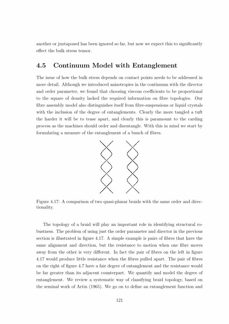
another or juxtaposed has been ignored so far, but now we expect this to significantly
effect the bulk stress tensor.
4.5 Continuum Model with Entanglement
The issue of how the bulk stress depends on contact points needs to be addressed in
more detail. Although we introduced anisotropies in the continuum with the director
and order parameter, we found that choosing viscous coefficients to be proportional
to the square of density lacked the required information on fibre topologies. Our
fibre assembly model also distinguishes itself from fibre-suspensions or liquid crystals
with the inclusion of the degree of entanglements. Clearly the more tangled a tuft
the harder it will be to tease apart, and clearly this is paramount to the carding
process as the machines should order and disentangle. With this in mind we start by
formulating a measure of the entanglement of a bunch of fibres.
Figure 4.17: A comparison of two quasi-planar braids with the same order and direc-tionality.
The topology of a braid will play an important role in identifying structural ro-
bustness. The problem of using just the order parameter and director in the previous
section is illustrated in figure 4.17. A simple example is pairs of fibres that have the
same alignment and direction, but the resistance to motion when one fibre moves
away from the other is very different. In fact the pair of fibres on the left in figure
4.17 would produce little resistance when the fibres pulled apart. The pair of fibres
on the right of figure 4.7 have a fair degree of entanglement and the resistance would
be far greater than its adjacent counterpart. We quantify and model the degree of
entanglement. We review a systematic way of classifying braid topology, based on
the seminal work of Artin (1965). We go on to define an entanglement function and
121

then a corresponding evolution equation for it. Finally we test the new model against
experiment
4.5.1 Degree of Entanglement and Braid Theory
We begin the process of quantifying the entanglement of a group of fibres by classifying
their braid topology. If we consider a bundle of n fibres, a braid is a three-dimensional
object that can be described topologically by a planar diagram. In this plane there
are two parallel lines where on each there lies a set of points Mi = (i, 0, 0) and
Ni = (i, 0, 1), a fibre will begin from a point Mk and end on the point Nl where the
fibres do not intersect on the two parallel lines. Between the two parallel lines the
fibres go over and under each other, see figure 4.18. In the planar braid diagram, one
always assumes that a strand descends without any regions of ascent from one parallel
line containing Mi’s to the other parallel line containing Ni’s. For each diagram we
can construct an infinite number of topologically equivalent three dimensional objects.
Artin (1965) began studying braids and showed that braids under the aforementioned
description form a group. We will use this theory as the basis for our description of
the inter-fibre knottedness.
MM1 2 M3 M4 MM1 2 M3 M4
NN N N1 2 3 4 NN N N1 2 3 4
A B
Figure 4.18: A couple of braid diagrams.
For a braid, the group operation is the product of two braids A and B. For an
n-braid group, Bn, each braid has n fibres or strands. In the planar diagram of a
three-dimensional braid we prescribe the beginning and end points to be equidistant.
The associative binary operation, the product, is the result of placing the top of B
at the bottom of A, see figure 4.19. The inverse of a braid, A, is simply the reflection
122

MM1 2 M3 M4
NN N N1 2 3 4
A
B
Figure 4.19: A diagram illustrating the product of two braids given in figure 4.18
at either one of the bounding parallel lines in the braid diagram. The unit element
is the braid where there are no cross-overs.
It is important to mention the equivalence class of braids. If there are two points
on a strand, bounded by x1 and x2, one can choose a third point, x3, that is not on
the chosen strand and change the original strand element from the original bounded
by x1 and x2, by using a polygonal link from x1 to x3 and then from x3 to x2. When
the polygonal links, x1 → x3 and x3 → x2, are always descending and if the surface
bounded by the polygonal links x1 → x2, x1 → x3 and x3 → x2 do not intersect
any other strand, we call this geometric deviation an elementary move. Two braids
are equivalent if one braid can be transformed into another braid by using elementary
moves. A corollary of this is that the product operation of three braids is associative.
......
... ...
i i+1
i i+1
bi−1
bi
Figure 4.20: A i-th braid generator and its inverse.
Now we progress on to developing the final piece of the braid topology jigsaw,
braid generators. We define a simple set of braid generators where there is only
123

one cross-over between two fibres, b1, ..., bn−1, see figure 4.20. Any braid in Bn
can be constructed using the generators as long as the representative diagram in the
projection plane is composed of cross-overs at different altitudes. When this latter
condition is violated we can find a representative case in the equivalence class that
will satisfy this condition. Now we consider some illustrations in order to find three
relationships between braid generators that allows us to migrate between equivalent
braids. This should also eliminate any ambiguity caused by the choice of projection
plane for the braid diagram.
1 2 3
3 2 1
1 2 3
2 2 1 3 2 1 3 2 1
3211 2 3 1 2 3
123 3 2 1
321
←→ ←→←→
Figure 4.21: Three couples of braids illustrating transformations that yield the braidrelation.
The first of three braid generator relationships is the simplest: a generator followed
by its inverse is equivalent to the identity braid. Topologically, they are simply fibres
standing side-by-side. A simple illustration is the braid on the left-hand-side in figure
4.17, and this gives the result
bib−1i = 1. (4.104)
Now we consider three pairs of braids that illustrate the braid relation, see figure 4.21.
Each pair is equivalent under elementary moves. The two equivalent braids on the
left of figure 4.21 give the relation
bibi+1bi = bi+1bibi+1. (4.105)
The other two transformations in figure 4.21 produce similar relational equalities
bibi+1b−1i = b−1
i+1bibi+1 and b−1i bi+1bi = bi+1bibi+1 respectively, and by using equation
(4.104) these equations are equivalent to (4.105). There remains just one more braid
generator relation to complete the picture. The property is called far commutivity.
We can see that the cross-overs in figure 4.22 can be moved up or down relative to
each other by using elementary moves, and so again are equivalent. This yields the
relationship:
bibj = bjbi whenever | i− j | ≥ 2. (4.106)
124

......... ... ......←→
Figure 4.22: Two couples of braids illustrating transformations that yield the farcommutativity relationship.
The braid relation and far commutivity are also known as Artin’s Braid Relations.
Prasolov and Sossinsky (1997) show that the braid group Bn is isomorphic to the
abstract group generated by the braid generators b1, ..., bn−1 that satisfy Artin’s Braid
Relations, (4.105) and (4.106). This gives a method of writing down the entanglement
of a braid.
Within the equivalence class of a braid, the member with the least number of braid
generators may be found and this we label as a canonical braid, and the set of these
braids we call ω. The canonical braid is not unique but equivalent canonical braids
will be composed of the same number of generators. We define entanglement, κ, to
be the number of generators found in the canonical braid per elementary volume. A
function, Ω can be defined, that operates on the set of canonical braids, ω, varying on
the interval Ω : ω → [0, a]. Furthermore, Ω is strictly monotonically increasing with
respect to the number of braid generators, such that for the identity element, i say,
Ω(i) = 0 and for the braid with the most generators, m say, Ω(m) = a. We write:
κ =Ω(B)
a, (4.107)
where a is a positive real number. One method of calculating Ω would be to choose
a spheroid centred on a point, then compose a braid with the fibres in the spheroid.
Another method for finding the braid that will define entanglement at a chosen point,
would be to include all fibres that are topologically tangled with fibres in the spheroid.
4.5.2 Governing Equations
The equations for conservation of mass (4.2) and momentum (4.31), kinematic con-
dition (4.63), evolution of order parameter (4.66), still hold. In addition to these we
modify the viscous coefficients (4.61) of the stress tensor (4.59) and introduce a new
equation for the evolution of the entanglement.
125

Figure 4.23: A couple of braids illustrating how extension of an element will intuitivelyreduce entanglement.
4.5.2.1 Empirical Law for Entanglement
We ignore the effect of extreme fibre clustering, what is known in the textiles industry
as “nep” formation, as this would coincide with spikes in the density and entangle-
ment functions. In the equation for directionality (4.63), we used the concept of a
group of fibres being moved relative to one another, where extensions were quanti-
fied by a length factor s. As this action occurs we also expect fibres to disentangle,
certainly if we ignore nep formation. Therefore we assume that the concentration
of entanglements will decrease, when material elements are stretched. The length
of fibres concerned will influence the rate at which the decrease occurs. We begin
by assuming a simple relationship and ensuring that the entanglement concentration
remains positive, we write:
∂κ
∂t+ (u · ∇)κ = −ακ1
s
[∂s
∂t+ (u · ∇)s
]. (4.108)
An illustration of the concept behind this equation (4.108) can be seen in figure 4.23.
We reiterate that this is not always the case as some braids will need more than just
simple local elongations in the direction a, in order to become less or completely
disentangled.
4.5.2.2 The Stress Tensor
For the stress tensor (4.59) we look to incorporate the additional information of the
fibres entanglement. When the fibres are highly tangled then they will resist stress
126

better than when fibres are only loosely connected. A simple polynomial relationship
is:
µi = κpρ2µi and λi = κqρ2λi, (4.109)
and a good starting point for this heuristic power law is p = q = 1. Notice that
the degree of entanglement is completely independent of the director and order, and
also braid topology is independent of density. Therefore our viscous coefficients in
(4.109) now include the important physical characteristics that describe a body of
fibres. Again we look to test the proposed continuum model against experiments
from section 4.2, tuft breakage force and tuft shear force.
4.5.3 Elongation of a Fibrous Mass
As in the case for the simple viscous model in section 4.3 and the model with order and
director 4.4.5, there are two parallel clamps holding the material that are separated
initially by a prescribed distance and we measure the force required to elongate the
material at a uniform velocity.
4.5.3.1 The Governing Equations
As in section 4.4.5 the problem can be simplified by constraining the motion to be in
one direction, so that v = 0 and the functions depend only on x and t. The governing
two dimensional equations, (4.68)–(4.75), then simplify to give:
∂ρ
∂t+
∂
∂x(ρu) = 0, (4.110)
∂θ
∂t+ u
∂θ
∂x= − cos θ sin θ
∂u
∂x, (4.111)
∂φ
∂t+ u
∂φ
∂x= β(1− φ) cos2 θ
∂u
∂x, (4.112)
∂κ
∂t+ u
∂κ
∂x= −ακ cos2 θ
∂u
∂x. (4.113)
As before in section 4.4.5, we constrain motion transverse to the direction of elonga-
tion by imposing (4.79).
4.5.3.2 Boundary Conditions
At the two solid boundaries we impose no-slip velocity conditions, where one bound-
ary, x = l(t), moves at a prescribed speed and the other at x = 0 is fixed, so
u = 0 at x = 0, (4.114)
and u = U at x = l(t). (4.115)
127

Initial conditions are then set for density, directionality and order:
ρ(x, t = 0) = ρ0(x), κ(ξ, t) = κ0(ξ) and φ(x, t = 0) = φ0(x). (4.116)
4.5.3.3 Dimensionless Lagrangian Formulation
We can solve this problem by using the same method as that used in section 4.3
and 4.4. Reformulation of the problem using Lagrangian variables and the creation
of dimensionless equations using the scalings of section 4.4, equations (4.2), (4.31),
(4.63), (4.66), (4.109) and (4.59) simplifying to
∂ρ
∂t= −ρ∂u
∂ξ
∂ξ
∂x, (4.117)
∂φ
∂t= β(1− φ)
∂u
∂ξ
∂ξ
∂x, (4.118)
∂κ
∂t= −ακ∂u
∂ξ
∂ξ
∂x, (4.119)
∂σ11
∂ξ= 0 (4.120)
where σ11 = γκρ2∂u
∂ξ
∂ξ
∂x[ν(1− φ) + φ] , (4.121)
respectively, where γ = ρ2Ul
and ν = AB+2C+D
. We note that the entanglement is a
dimensionless variable already. The boundary conditions become
u(0, t) = 0, u(1, t) = 1, (4.122)
ρ(ξ, 0) = ρ0(ξ), κ(ξ, 0) = κ0(ξ) and φ(ξ, 0) = φ0(ξ). (4.123)
Now we drop the dimensionless notation, removing the over-bars. We can now find
relationships between three of the four unknowns by eliminating ∂u∂ξ
∂ξ∂x
in equations
(4.117)–(4.119) and integrating, to get
φ(ξ, t) = 1 + (φ0(ξ)− 1)
(ρ(ξ, t)
ρ0(ξ)
)β(4.124)
= 1 + (φ0(ξ)− 1)
(κ(ξ, t)
κ0(ξ)
) βα
. (4.125)
To find the solution of the differential equations (4.117)–(4.120) with boundary con-
ditions (4.122) we need to integrate equation (4.120) and use equation (4.117):
−ρ(ξ, t)α+1
ρ0(ξ)α
[1 + (1− ν)(φ0(ξ)− 1)
(ρ(ξ, t)
ρ0(ξ)
)β]∂ρ(ξ, t)
∂t= F (t) (4.126)
where F (t) is the force prescribed at one end of the tuft, i.e. ξ = l.
128

4.5.3.4 The Solution For a Uniformly Dense Tuft
Similar to the problem solved in section 4.4, a much simpler form can be deduced if we
assume a constant initial density, order φ0 and entanglement κ0. This means that in
the Lagrangian framework, all the characteristic variables except velocity will depend
on time only. Using the boundary condition (4.122) and by writing X(ξ, t) = 1 + t,
the explicit solutions are:
ρ(t) =1
1 + t, (4.127)
φ(t) = 1 +φ0 − 1
(1 + t)β, (4.128)
κ(t) =κ0
(1 + t)α, (4.129)
F (t) =κ0
(1 + t)3+α
[1 +
(1− ν)(φ0 − 1)
(1 + t)β
]. (4.130)
The dimensionless density from equation (4.127), still tends monotonically to zero as
time tends to infinity. The order and entanglement both depend on one parameter,
and their respective initial conditions. Order tends to one and entanglement tends
to zero as time progresses, but we have now introduced κ0 and the exponent α which
allows more flexibility in matching F (t) with experiment.
Finally the force produced at the moving boundary as a consequence of the motion
is given in equation (4.130). A turning point for F occurs at
tmax =
((1− ν)(1− φ0)(3 + α + β)
3 + α
) 1β
− 1. (4.131)
One condition for a maximum to exist, when tmax ≥ 0, is ν < 1, and this means that
the nematic component of the stress tensor should dominate over the isotropic part
in terms of their respective contributions to the bulk stress. Moreover we require:
(1− ν)(1− φ0) >3 + α
3 + α + β, (4.132)
and as the disparity in the inequality increases (i.e. ν gets smaller), tmax moves away
from the origin. For the same material where α, β and ν are the same then the
initial order of the material is the only parameter that influences the position of the
maximum, whereas the initial entanglement effects the magnitude of the resistive
force linearly. The height of the maximum is:
Fmaxκ0
=
[3 + α
(1− ν)(1− φ0)(3 + α + β)
] 3+αβ(
β
3 + α+ β
). (4.133)
129

Local analysis near the turning point, indicates that the behaviour will always be
a maximum provided α, β ≥ 0. The equation (4.132) suggests that if the rate at
which the order parameter evolves is large (β 3 +α), then the later the maximum
occurs in the experiment and also the smaller its the magnitude. We note that if the
maximum point doesn’t exist, tmax < 0, then the behaviour is similar to the “simple”
viscous model given in section 4.3.
The results for density, order, entanglement and force given by (4.127)–(4.130),
have been plotted, see figures 4.24 and 4.25 for the results. The dimensional force
from (4.130) is
Fdim(t) =κ0(B + 2C +D)ρ2
0lα+2U
(l + Ut)3+α
[1− (1− ν)(1− φ0)lβ
(l + Ut)β
]. (4.134)
We note that the initial force for the experiment that includes entanglement (4.130)
is the same as (4.103) except that it is multiplied by the initial knottedness κ0. This
implies that for the same entanglement, the initial force required to elongate a tuft
will increase linearly with φ0. Now we have the ability to differentiate between a
combed group of straight fibres and an entangled group of straight fibres, where the
latter produces greater resistance to elongation. Moreover any group of fibres that
are highly tangled κ ∼ 1 will now produce greater resistance to viscous deformations
than a group of fibres that are well combed (κ ∼ 0).
4.5.3.5 Comparison with Experiment
When the initial tuft size length varies in the tuft breaking force experiment, see
figure 4.25 plots (a) and (b), the qualitative comparison between experiment and
mathematical simulation can be very good by choosing α and β appropriately. As
our analysis shows we can change numerous parameters, for example α and β, that will
depend on the chosen material, and we have chosen our results to fit the experiment
for polyester.
For the variable speed tuft breaking experiment, see figure 4.25 plots (c) and
(d), the comparison is less good. As mentioned in section 4.2, it is quite likely that
the results recorded include noise produced by the difficultly in obtaining equivalent
tufts for each test. In terms of the model, for the same material, the initial order,
entanglement and director may differ. All these parameters would also significantly
change the mathematical simulation. Regardless of the possibly spurious comparative
data the qualitative shape of the curves are similar in the aforementioned plots.
130

1 2 3 4 5time
0.2
0.4
0.6
0.8
1Order
(a) β = 1 and φ0 = 0, 0.2, .., 1.
1 2 3 4 5time
0.2
0.4
0.6
0.8
Order
(b) β = 0.2, 0.6, ..., 1.8 and φ0 = 0.1
1 2 3 4 5time
0.2
0.4
0.6
0.8
1Entanglement
(c) α = 1 and κ0 = 0.2, 0.4, ..., 1.
1 2 3 4 5time
0.2
0.4
0.6
0.8
Entanglement
(d) α = 1.8, 1.4, ..., 0.2 and κ0 = 1.
Force
00.1
0.20.3
0.40.5
time0
0.2
0.4
0.6
0.81
nu0
0.250.5
0.751
00.1
0.20.3
0.40.5
time
(e) κ0 = 1, φ0 = 0.01, α = 1, β = 25.
Force
00.5
11.5
2
time0
0.1
0.2
0.30.40.5
beta0
0.020.040.06
00.5
11.5
2
time
(f) κ0 = ν = 0.01 and φ0 = κ0 = 1.
Figure 4.24: Results of the dimensionless elongation problem for the continuummodel: (a) and (b) are plots of the order parameter, (c) and (d) are plots of theentanglement, and (e) and (f) are plots of the force. The graphs with multiple func-tions correlate to the given values beneath the graph in ascending order.
131

10 20 30 40 50 60time
0.2
0.4
0.6
0.8
Force
(a) κ0 = α = β = 1, U = 5610−3m/s,
φ0 = ν = 0.01, l = 0.04, 0.03, 0.02, 0.01m.(b) Experiment for polyester with vari-able initial lengths: force against exten-sion.
5 10 15 20time
0.5
1
1.5
2
Force
(c) κ0 = α = β = 1, l =0.04m, φ0 = ν = 0.01, U =5610−3, 10
6 10−3, 406 10−3, 50
6 10−3m/s.
(d) Experiment for polyester with vari-able elongation velocity.
5 10 15 20 25time
0.050.1
0.150.2
0.250.30.35
Force
(e) φ0 = 0.01, κ0 = α = 1, l = 0.01m,U = 5
610−3m/s, β = 0, 0.1, 0.2, 0.3.
10 20 30 40time
0.5
1
1.5
2
2.5
3Force
(f) κ0 = α = β = 1, φ0 = 0.01, l = 0.01m,U = 5
610−3m/s, ν = 0.05, 0.15, 0.25, 0.35.
Figure 4.25: Results of the dimensional elongation problem for the continuum model:(a) and (b) compares experiment with mathematical simulation for varying gaugelengths, (c) and (d) is a comparison for varying velocity. The functions on each graphcorrelate to the given values below where the respective plots in ascending order.
132

4.5.4 A Simple Shearing Problem
0 0 0 0 0 0 0 0 0 0 0 00 0 0 0 0 0 0 0 0 0 0 00 0 0 0 0 0 0 0 0 0 0 00 0 0 0 0 0 0 0 0 0 0 00 0 0 0 0 0 0 0 0 0 0 00 0 0 0 0 0 0 0 0 0 0 00 0 0 0 0 0 0 0 0 0 0 00 0 0 0 0 0 0 0 0 0 0 00 0 0 0 0 0 0 0 0 0 0 0
1 1 1 1 1 1 1 1 1 1 11 1 1 1 1 1 1 1 1 1 11 1 1 1 1 1 1 1 1 1 11 1 1 1 1 1 1 1 1 1 11 1 1 1 1 1 1 1 1 1 11 1 1 1 1 1 1 1 1 1 11 1 1 1 1 1 1 1 1 1 11 1 1 1 1 1 1 1 1 1 11 1 1 1 1 1 1 1 1 1 1
2 2 2 2 2 2 2 2 2 2 22 2 2 2 2 2 2 2 2 2 22 2 2 2 2 2 2 2 2 2 22 2 2 2 2 2 2 2 2 2 22 2 2 2 2 2 2 2 2 2 22 2 2 2 2 2 2 2 2 2 22 2 2 2 2 2 2 2 2 2 22 2 2 2 2 2 2 2 2 2 22 2 2 2 2 2 2 2 2 2 2
3 3 3 3 3 3 3 3 3 3 33 3 3 3 3 3 3 3 3 3 33 3 3 3 3 3 3 3 3 3 33 3 3 3 3 3 3 3 3 3 33 3 3 3 3 3 3 3 3 3 33 3 3 3 3 3 3 3 3 3 33 3 3 3 3 3 3 3 3 3 33 3 3 3 3 3 3 3 3 3 33 3 3 3 3 3 3 3 3 3 3
FIXED
MOVING
FIXED
MOVING
Figure 4.26: A diagram of the shearing problem.
We continue testing this mathematical model by considering the shearing problem,
see figure 4.26. The material is now sheared by two parallel solid boundaries. If the
two plates bounding the material are smooth, there would no change during the
motion or very little non-recoverable change. One should witness constant slipping
between the fibres and the solid surface, unless the surface is rough or sticky. Small
hooks would produce the desired effect of shearing the material. A mathematical
simulation, where we attach the fibres to the solid boundary, could mimic events in
the carding machine or the experiment discussed in section 4.2. The effectiveness of
the model will depend on the hooks used in the experiments, moreover their ability
to hold onto fibres and in the model below we take the boundary condition to be a
no-slip on the wall, i.e. we neglect the effect of the hooks within the fibres.
4.5.4.1 The Governing Equations
As in paragraph 4.5.3 we constrain the motion to be in one direction, and we assume
that the initial state is uniform in the x-direction, allowing only for variations in time
and in y, and assuming v = 0. The director is written as a = (cos θ, sin θ, 0)T . The
governing equations from (4.68) – (4.75), become
∂ρ
∂t= 0, (4.135)
∂θ
∂t= − sin2 θ
∂u
∂y, (4.136)
∂φ
∂t= β(1− φ) sin θ cos θ
∂u
∂y, (4.137)
∂κ
∂t= −ακ sin θ cos θ
∂u
∂y. (4.138)
133

This means that the density does not evolve in time but could depend on the spatial
variable y. Equations (4.71) and (4.72) become:
∂
∂y
ρ2κ
∂u
∂y
[µ1(1− φ) + φ
(λ1 +
λ3
2+ λ5 sin3 θ cos θ
)]= 0, (4.139)
∂
∂y
ρ2κφ
∂u
∂y
[(λ1 + λ2) sin θ cos θ + λ3 sin3 θ cos θ
]= 0. (4.140)
Unlike the extensional problem we do not have to impose a condition on the director
because in this problem the fibre material is bounded by two solid “walls” and there
is no need to ensure that there is no transverse forces. The boundary and initial
conditions are simply no slip at the solid boundaries and initial conditions for density,
order and the director:
u = 0 at y = 0, u = U at y = h, (4.141)
κ(y, t) = κ0(y), θ(y, t) = θ0(y), φ(y, t) = φ0(y) at t = 0. (4.142)
Now we can progress to writing the equation in dimensionless form.
4.5.4.2 Dimensionless Formulation
Velocity is scaled with the speed of the moving solid boundary U , so u = Uu. To
scale density we use a constant ρ0 characterising the prescribed initial condition, so
that ρ = ρ0ρ. The entanglement and order are defined as normalised variables and
the angle θ is order unity. The typical length-scale of motion is distance between the
two parallel plates, so y = hy and finally we are left with scaling time conventionally
as t = hUt. The dimensionless equations (4.135)–(4.138) are:
∂θ
∂t= − sin2 θ
∂u
∂y, (4.143)
∂φ
∂t= β(1− φ) sin θ cos θ
∂u
∂y, (4.144)
∂κ
∂t= −ακ sin θ cos θ
∂u
∂y, (4.145)
and conservation of momentum equations (4.139) and (4.140) become:
∂
∂y
ρ2κ
∂u
∂y
[ν1(1− φ) + φ
(1 + ν2 + ν3 sin3 θ cos θ
)]= 0, (4.146)
∂
∂y
ρ2κφ
∂u
∂y
[(1 + ν4) sin θ cos θ + 2ν2 sin3 θ cos θ
]= 0, (4.147)
134

where ν1 = µ1
λ1, ν2 = λ3
2λ1, ν3 = λ5
λ1, and ν4 = λ2
λ1. The boundary and initial conditions,
from equations (4.141) become:
u = 0 at y = 0, u = 1 at y = 1. (4.148)
and equations (4.142) remain the same. We now drop the dimensionless notation for
tidiness, i.e. do not write the over-bars any more.
4.5.4.3 The Solution
1 2 3 4 5time
0.25
0.5
0.75
1
1.25
1.5
Director Angle
(a) θ0 = π8 ,
π4 , ..,
π2
0.2 0.4 0.6 0.8 1time
0.2
0.4
0.6
0.8
1Entanglement
(b) θ0 = π8 ,
π4 , ..,
π2
0.2 0.4 0.6 0.8 1time
0.2
0.4
0.6
0.8
1Order
(c) θ0 = π8 ,
π4 , ..,
π2
1 2 3 4 5time
0.6
0.7
0.8
0.9
Order
(d) φ0 = 0.2, 0.4, ..., 1.8
Figure 4.27: Results of the dimensionless shearing problem for the continuum model:(a) a plot of the director, (b) entanglement, (c) and (d) order. The plots on eachgraph correlate to the number written below each graph in ascending order.
By considering partial differential equations (4.143)–(4.145), we look for solutions
in which κ, φ and θ are only time dependent. This allows us to integrate equations
(4.146) and (4.147) with respect to y to give the velocity:
u =f1(t)y
ρ2κ[ν1(1− φ) + φ
(1 + ν2 + ν3 sin3 θ cos θ
)] + g1(t) (4.149)
135

u =f2(t)y
ρ2κφ[(1 + ν4) sin θ cos θ + ν2 sin3 θ cos θ
] + g2(t) (4.150)
respectively. Applying the boundary conditions (4.148) gives a simple linear velocity
profile, analogous to Couette Flow (see Batchelor (1967)),
u = y. (4.151)
Now with equation (4.151), the partial differential equations in (4.143) – (4.145)
become ordinary differential equations in time. The solutions are:
θ = arccot(t+ cot θ0), (4.152)
φ = 1 + (φ0 − 1)
[1 + cot2 θ0
1 + (cot θ0 + t)2
] β2
, (4.153)
κ = κ0
(1− φ0
1− φ
)αβ
= κ0
[1 + cot2 θ0
1 + (cot θ0 + t)2
]α2
, (4.154)
and we note that in this case that the density is constant. The director, regardless of
initial condition, will always tend to align itself parallel to the shearing boundaries.
Order evolves to the nematic phase, φ → 1, but depends on the initial direction
of the fibres, θ0. Similarly for the entanglement, we see an evolution that eliminates
knottedness but the rate at which this occurs depends on the initial director. For plots
of the functions (4.152)–(4.154) see figure 4.27. Two components of force (F,G)T are
found using the stress tensor,
F (t) =
(1 + cot2 θ0
1 + (t+ cot θ0)2
)α2
ν1(1− φ0)
(1 + cot2 θ0
1 + (t+ cot θ0)2
)β2
+
[1− (1− φ0)
(1 + cot2 θ0
1 + (t+ cot θ0)2
)β2
]
×[1 + ν2 +
ν3(t+ cot θ0)
[(t+ cot θ0)2 + 1]2
](4.155)
and
G(t) =
[1 + cot2 θ0
1 + (t+ cot θ0)2
]α2
[1− (1− φ0)
(1 + cot2 θ0
1 + (t+ cot θ0)2
)β2
]
×[
(1 + ν4)(t+ cot θ0)
1 + (t+ cot θ0)2+
ν2(t+ cot θ0)
[(t+ cot θ0)2 + 1]2
]. (4.156)
The dimensional forces are found by rescaling time with Ul
and multiplying the force
by ρ2B Ul, see figure 4.28. Now it remains to compare the results with experimental
data.
136

Force in the x-direction
02
46
810
time0.5
1
1.5
theta_00.40.60.8
02
46
810
time
(a) φ0 = ν1 = 0.1, α = β = 1, ν2 = ν3 =2.
Force in the y-direction
02
46
810
time0.5
1
1.5
theta_00
0.20.40.6
02
46
810
time
(b) φ0 = 0.1, α = β = 1, ν2 = ν4 = 2.
2 4 6 8 10time
0.1
0.2
0.3
0.4
0.5
Force
(c) Model with varying hook distances:l = 0.001, 0.002, .., 0.004m, U =0.001m/s.
(d) Shear force experiment for cottonwith varying hook-to-hook distance andshear speed of 100mm/min.
2 4 6 8 10time
0.1
0.2
0.3
0.4
0.5
0.6
Force
(e) Model with varying shear speeds: U =0.001, 0.002, .., 0.005m/s, l = 0.004m.
(f) Shear force experiment for cotton withvarying hook-to-hook distance and shearspeed of 200mm/min.
Figure 4.28: Force graphs for continuum model and the shearing experiment. Thepairs juxtaposed in this figure are simulations and their corresponding experiment.
137

4.5.4.4 Comparison with Experiments
The comparisons juxtaposed in figure 4.28 are fairly good. The main discrepancy is
that the experimental graphs show a greater decrease in the measured forced after
their respective maxima are reached. We can account for this, as the mathematical
model is based on an infinite channel of fibrous material and the experiments are
conducted with tufts, a cluster of fibres. This means that for the mathematical
simulation the density remains constant throughout, which is not what we would
expect in reality. It is also conceivable that as entanglement decreases the hooks’
ability to hold the fibres will diminish, and this suggests that the no-slip condition
may not be valid. The qualitative initial shape of the force plots is captured well with
the model, except for the previously documented fact that the force never begins at
zero, as explained in section 4.5.3.
4.5.5 An Array of Hooks
Another method of modelling the “shear force” experiment, is considering the hooks
as a body force acting on the continuous medium. For a viscous Newtonian fluid,
an array of fibres moving normal to the flow is modelled by Terrill (1990). In this
work, the author incorporates a body force on the fluid due to the presence of a
homogeneous uniform array of fibres, which are considered as a large number of long
slender cylinders to leading order. We have already transposed this problem before
by letting the cylinders represent hooks in section 2.4.
4 4 4 4 4 4 4 4 4 4 4 4 4 4 44 4 4 4 4 4 4 4 4 4 4 4 4 4 44 4 4 4 4 4 4 4 4 4 4 4 4 4 44 4 4 4 4 4 4 4 4 4 4 4 4 4 44 4 4 4 4 4 4 4 4 4 4 4 4 4 44 4 4 4 4 4 4 4 4 4 4 4 4 4 44 4 4 4 4 4 4 4 4 4 4 4 4 4 44 4 4 4 4 4 4 4 4 4 4 4 4 4 44 4 4 4 4 4 4 4 4 4 4 4 4 4 44 4 4 4 4 4 4 4 4 4 4 4 4 4 44 4 4 4 4 4 4 4 4 4 4 4 4 4 44 4 4 4 4 4 4 4 4 4 4 4 4 4 44 4 4 4 4 4 4 4 4 4 4 4 4 4 44 4 4 4 4 4 4 4 4 4 4 4 4 4 4
5 5 5 5 5 5 5 5 5 5 5 5 5 5 55 5 5 5 5 5 5 5 5 5 5 5 5 5 55 5 5 5 5 5 5 5 5 5 5 5 5 5 55 5 5 5 5 5 5 5 5 5 5 5 5 5 55 5 5 5 5 5 5 5 5 5 5 5 5 5 55 5 5 5 5 5 5 5 5 5 5 5 5 5 55 5 5 5 5 5 5 5 5 5 5 5 5 5 55 5 5 5 5 5 5 5 5 5 5 5 5 5 55 5 5 5 5 5 5 5 5 5 5 5 5 5 55 5 5 5 5 5 5 5 5 5 5 5 5 5 55 5 5 5 5 5 5 5 5 5 5 5 5 5 55 5 5 5 5 5 5 5 5 5 5 5 5 5 55 5 5 5 5 5 5 5 5 5 5 5 5 5 55 5 5 5 5 5 5 5 5 5 5 5 5 5 5MOVING
FIXED
Hook-Entrained Region
Shear Region
Hook-Entrained Region
Figure 4.29: A diagram of the fibre continuum which is sheared by two arrays parallelhooks.
For our non-Newtonian viscous material, which is composed of fibres we can add
a body force to the momentum equation (4.3) which is due to the movement of hooks
138

through the fibrous material. In the work by Terrill (1990), the approximation is for
slow flow, and in our case the fibres behave in a similar way, i.e. Λ 1. From our
work in section 2.4 we could think of the approximation (2.31) as the sum of the
forces produced by one hook in low Reynolds number flow:
fi = Huiδ(x− xhook), (4.157)
where H is a viscous coefficient, ui is relative velocity and xhook is the position of the
hook. The forces (4.157) can be added into the equation of conservation of momentum
(4.31) to produce a body force on the fibre continuum proportional to the velocity of
the fibres relative to the hooks. When the forces produced by the hooks dominate over
inertia and viscous stresses, fibres will be entrained by the shearing surfaces, and there
will be a region of shear in between the two hook layers. This means that our shearing
calculations of section 4.5.2 would then be useful in the gap region. Consequently
one approximation that includes hooks will produce exactly the same results as the
shearing experiment in section 4.5.4, as the two entrained fibre regions create two no
slip conditions at interfaces between the shear-region and the hook-entrained regions,
see figure 4.29.
4.6 Conclusion
We have identified three potential areas of applied mathematics and theoretical
physics that model “microscopic” nematic structures, namely liquid crystals, fibre
reinforced fluids and polymers. Within all these fields there is one unifying method-
ology and that is the use of continuum models and the idea of a director. None of
the theories and techniques migrated well enough to model fibre deformations in the
carding machine so we designed a new continuum model where the dominant physical
mechanism was friction between fibres. The key prescribed concepts were that the
material’s dominant behaviour in the carding machine was viscous and that these
deformations occurred under tension.
Using just velocity and density to describe a many-fibre body, we began to explore
the possibilities of finding a tractable model. An isotropic bulk stress tensor was
carefully derived using a probabilistic technique, where the viscous coefficients were
proportional to the square of density. Comparisons with experiment and our model
partially justified the viscous assumption as there was a fair degree of similarity,
but the theoretical simulations failed to capture the behaviour of a fibre-medium
139

when forces are initially applied. We postulated that this was due to the lack of
directionality and anisotropy in the model.
After defining two new continuum quantities, the order parameter and director, we
defined a kinematic condition and an empirical evolution equation. A new bulk stress
tensor incorporated both isotropic and anisotropic components, where the latter was
based on transversely isotropic media. The comparison with experiments improved
significantly as we captured, qualitatively, the behaviour of a many-fibre material as
it was being elongated, in particular during the initial stages of the experiment. This
result however, was not so conclusive when one looked closely at the relationship
between initial order and the magnitude of the force produced. It was clear that
neglecting how the fibres were interconnected led to counter-intuitive results.
Finally we introduced a function that defined the degree of entanglement. An
explanation of the required braid theory was followed by the introduction of a new
evolution equation for entanglement, and the viscous coefficients of the bulk stress
were modified. The comparisons with experiments, for both elongational and shear-
ing cases, were very promising. We have established a model for many-fibres, in-
terconnected and entangled deformed under tension, that incorporates alignment,
directionality and entanglement. All of these three characteristics are vital to textile
engineers.
140

Chapter 5
Conclusions
We have created a number of models that provide insight into and understanding of
the principal physical processes and mechanisms of the carding machine. We have
done this by applying a number of areas of classical mechanics in novel settings
and created an original model for a many-fibre-medium. Numerous methodologies
were employed from perturbation theory to braid topology. There were three key
areas of interest that arose from conversations with industrialists and experimental-
ists involved with textile manufacturing processes. These were: the behaviour of
a single fibre in the carding machine, in particular their transfer between surfaces,
the behaviour of fibre being teased out of tufts, and a macroscopic model for many
interconnected fibres.
In chapter 2 we derived a model for a textile fibre in the carding machine, which
included rotational and aerodynamic forces. We ignored any interaction with other
fibres and focussed on fluid flow and hook-fibre friction. Working from the simplest
scenario, where a fibre is tethered by a hook on a rotating drum, we examine the
issue of fibre transfer between carding surfaces. The fibres would lie close to the
hooked-drum surface from which it was being tethered, except when the fibre entered
the nip regions between taker-in and cylinder and also cylinder and doffer. In these
two nip regions, we found mechanisms for transfer were completely different.
The work in chapter 3 considered how a fibre is extracted from a tuft. We decou-
pled the internal forces within the tuft and the tension in the fibre. Then we went
on to consider how a tuft, when sheared or teased can be modelled by two tufts with
inter-connecting fibres. This work illuminates the forces acting on a fibre as it moves
through a mass of fibres in a tuft.
The assumption, that fibre withdrawal does not affect the tuft structure, was not
adequate when considering many interconnecting fibres and so in chapter 4, we create
a continuum model for many interacting fibres. We introduced an order parameter, a
141

director and an entanglement function. The governing equations were derived using
the mathematics from subjects such as transverse isotropic symmetry in continuum
models and braid theory. The limitation to the model from the industrialist’s point of
view was that we could not incorporate the possibility of nep formation, singularities
in the entanglement function. The mathematical model compared very well with
experimental data, which included an elongational and shearing problem. Now we go
on to describe how all the aforementioned models cumulatively describe the transport
and deformation of fibres in the carding process.
5.1 The Life of Fibres in the Carding Machine
6767676767676767667676767676767676676767676767676766767676767676767667676767676767676676767676767676766767676767676767667676767676767676676767676767676766767676767676767667676767676767676
8787878787878787887878787878787878878787878787878788787878787878787887878787878787878878787878787878788787878787878787887878787878787878878787878787878788787878787878787887878787878787878
Taker-in(d)
(c)
Cylinder
(b)
(a)
Doffer
Cylinder
(e)
(f)
(g)(h)
(i)
Figure 5.1: Diagrams illustrating the life of a single fibre in the carding machine.
142

5.1.1 The Taker-In
The taker-in teases out a single fibre from the lap on the feeder-in or it will grab a
tuft, see (a) in figure 5.1 and (i) in figure 5.2. In both cases we can apply the models
of chapter 3, that is the single fibre withdrawal problem from a tuft and two tufts with
interconnecting fibres. From the solutions we can then predict fibre breakage based
on the machine setting and the degree of entanglement in the lap. The continuum
model of chapter 4 could also be applied to this region, because as the fibres are fed
onto the taker-in, the rotation of the taker-in shears the fibre mass. Our continuum
model can predict how the order in the fibre-medium evolves from this shearing.
It is found experimentally that half the fibres on the taker-in do not interact
with other fibres. For the single fibres we can use the models of chapter 2, where
we expect the fibres to remain close to the drum surface (b) until they reach the
nip region between taker-in and doffer, the single fibre transfer onto the cylinder by
the leading end first, see point (c) in figure 5.1. This mechanism is governed by the
aerodynamics as described in section 2.5. As the tufts transfer onto the cylinder there
may be slight changes in their respective structure which would be generated by the
shearing motion in the nip region, see (ii) in figure 5.2. The reason for assuming that
the changes are slight is that the hooks on both surfaces in the nip region all face the
same direction, and consequently the resistance to motion relies on the ability of the
taker-in hooks to hold onto a tuft, and this will be minimal.
5.1.2 The Cylinder
Tufts that enter the carding region have already been teased by their extraction
from the lap with the taker-in hooks. The fixed and revolving flats now produce
considerable resistance to tufts that are transported through this region, see (iii) in
figure 5.2. Here we can apply the shearing problem of chapter 4 for a continuous
media. We can use the machine parameters in our model to approximate how the
tufts will evolve through this part of the process, although in order to find some of
the parameters in the model, we will require experimental data. Single fibres, as
they enter the region with the revolving and fixed flats, will remain close to the drum
surface (see (e) in figure 5.1), and they should not interact with neighbouring machine
surfaces. By the end of the revolving flats, from section 1.1, all the tufts should be
broken down into individual fibres.
All the fibres now can be treated as single fibres, and modelled by the equations
in chapter 2. The transfer mechanism from cylinder to doffer is also governed by
143

999999
:::::
;<;<;;<;<;;<;<;;<;<;;<;<;
=<=<==<=<==<=<==<=<==<=<=(i)
><><><><>><><><><>><><><><>><><><><>><><><><>><><><><>><><><><>><><><><>><><><><>
?<?<?<?<??<?<?<?<??<?<?<?<??<?<?<?<??<?<?<?<??<?<?<?<??<?<?<?<??<?<?<?<??<?<?<?<?
@<@<@@<@<@@<@<@@<@<@@<@<@@<@<@@<@<@@<@<@
A<AA<AA<AA<AA<AA<AA<AA<A
(ii)
(iii)
Taker-in
Cylinder
Figure 5.2: A diagram illustrating the regions where entangled tufts are teased intoindividual fibres or evolve into less entangle tufts.
the fluid dynamics, and the tails of the fibres are offered to the doffer hooks, see (f)
in figure 5.1. Some fibres transfer onto the doffer and some remain on the cylinder.
Those that remain on the cylinder, see (g) in figure 5.1 will always remain close to the
cylinder surface until they return to the doffer nip region where they will be offered
again for transfer.
5.1.3 The Doffer
Fibres that transfer onto the doffer are then transported to the stripper, which takes
the fibres out of the machine in the form of the sliver, see (j) in figure 5.1. We modelled
a single fibre on the doffer in chapter 2, see (h) in figure 5.1. All these models can
help carding machine manufacturers, by firstly explaining how fibres evolve and move
throughout the machine and then by using the theoretical simulations to suggest
optimal hook design, machine settings and machine geometries.
5.1.4 Suggested Further Work
For the single fibre model, the main difficulty arose from finding the correct fluid
flow. For both annular and transfer regions improvements could be made to our
144

aerodynamic approximations. In the case of annular flow, the incorporation of the
hooks assumed that the hooks were cylindrical and not radially dependent. This
is not the case for the cylinder, doffer and taker-in hooks. The hooks are usually
thin triangular prisms. This may give a radial dependence for the amount of fluid
entrained by the hooks, which will in turn affect the aerodynamic forces acting on the
fibre. Other modifications could be made by considering the viscous model to flow
around the two cylinders, and to quantify the level of local instability on a fibre due
to turbulence.
There is much more work that could be done on the fibre withdrawal problems
and the continuum model. The issue of modelling inter-fibre dynamic friction could
be addressed in a number of ways, but the outcome of any such study will benefit
both models in chapters 3 and 4. For the two tufts with many interconnecting fibres it
is not clear whether or not a change in the body force would have made the solutions
more realistic. We could also couple the fibre withdrawal problem with the fibre
continuum, and this would hopefully explain the differences in the fibre elongation
experiment and the breaking of two tufts with interconnecting fibres.
The main area that would benefit from more analysis is the continuum model of
chapter 4. There are three important areas. The first would be to compute the size of
the unknown parameters in the model and this could be achieved by constructing a
number of experiments. This may require further simulations of the model which will
require numerical computation. The second would be theoretical improvements to the
empirical laws that govern the evolution of the order parameter and the entanglement
scalar field. For the empirical laws, in particular the evolution of entanglement, one
may be able to consider the braid topologies so that they understand structural
evolution of a tuft under the various stresses.
145

Appendix A
Dimensional and DimensionlessNumbers
A.1 Drum Speeds
The specifications of the three main cylindrical drums inside the revolving-flat carding
machine.
Unit Taker-In Cylinder Doffer
Diameter metres 0.25 1.0 0.5Revolutions rpm 600 – 1500 500 – 750 25 – 100Surface Speed metres per minute 471.2 – 1178 1570 – 2356 39.27 – 157.1
metres per second 7.854 – 19.63 26.18 – 39.27 0.6545 – 2.618
Table A.1: Drum specifications.
A.2 The Fibres
Two commonly used short-staple fibres are cotton and polyester, and a description
of their properties are given in table A.2. The average typical mass flow of polyester
through the carding machine is about 12
kg/min.
A.3 Fluid Dynamics and Drag
We compute the Reynolds number, Re = ULν
, using the circumference of the cross
section of the drum, the surface speed of the cylinder and the kinematic viscosity,
ν = 0.150 cm2/sec, for air at twenty degrees Celsius, found in Batchelor (1967) on
146

Cotton PolyesterLength 20.0–48.0 mmAverage Length 28 mm 38 mmDiameter 11.5–22.0 micronAverage Diameter 17 micron 6.26 micronweight 6.832 10−6 g 6.46 10−6 gAverage Density 1.075 106 g/m3 5.784 106 g/m3
Moment of Inertia I =∫Ar2dA 8.2 10−21 m4 1.508 10−22 m4
Young’s Modulus E 9 109 N/m2 7.7 109 N/m2
Table A.2: The properties of cotton and polyester Fibres.
page 594. For the local Reynolds number near the fibre we consider the circumference
of the fibre. A polyester fibre has an approximate diameter of 6.26 microns. We
estimate the thickness of the boundary layer, in metres, on an infinite smooth cylinder
to be δ = O( l√Re
), where l is the typical length, see Rosenhead (1963).
Reynolds No. Taker-In Cylinder Doffer
Cylinder 4.1× 10⁵–106 5.5× 10⁶–8.2× 10⁶ 6.9× 10⁵– 2.7× 10⁵
Single fibre 10–26 34–51 0.86–3.4
Boundary layer 7.8× 10⁻⁴–1.2× 10⁻³ 1.1× 10⁻³–1.3× 10⁻³ 3.0× 10⁻³– 6.0× 10⁻³
Table A.3: The Reynolds numbers of a drum in a homogeneous fluid.
A.3.1 Stokes Drag
The slow flow approximation for flow around a cylinder breaks down (Khayat and
Cox, 1989), when
∣∣∣∣lnRe− ln ε
(ln ε)2
∣∣∣∣∣∣∣∣
1
ln ε
∣∣∣∣ . (A.1)
Considering a polyester fibre with aspect ratio ε = al
= 0.000824, then ln ε = −2.497
and we find that (A.1) is true only for the doffer.
In chapter 2, a single fibre in Stokes flow was discussed. The important dimen-
sionless parameter κ = 8AρairaReρfibre log 1
ε
, see table A.4, is the ratio of centrifugal force
over viscous drag, where A is the radius of the rotating drum, a is the radius of the
fibre, Re is the Reynolds number for flow around the fibre, and ρair and ρfibre are the
respective air and fibre densities.
147

Doffer
κ 6.22× 10⁵ – 2.48× 10⁶
Table A.4: Dimensionless parameter κ for a single fibre with Stokes drag.
A.3.2 Taylor Drag
In section 2, a fibre on the cylinder and taker-in involved the dimensionless parameter
ς, which was the ratio of Taylor drag over centrifugal force. The two definitions
used are dependent on the local flow, “triple-layer” and shear flow, and these were
ς =2πa(B−A)2ρfibre
Al2ρairand ς =
2πaρfibreAρair
respectively, see table A.5.
ς Taker-In Cylinder
“triple-layer” flow 1.27× 10⁻⁴ 5.01× 10⁻⁴
shear flow 1.41× 10⁻⁵ 5.57× 10⁻⁵
Table A.5: Dimensionless parameter ς for single polyester fibre with Taylor drag.
148

Appendix B
Shear Breaking Experiments onTufts
In section 4.2, the “tuft shear force” experiment was described. A tuft is placed
between two wired surfaces where one traversed the other at a uniform velocity. The
distance between the hooks were varied (0.007, 0.01 and 0.013 inches), as well as
the relative velocity of surfaces (50, 100 and 200 mm/min). There are three sets of
experiments for cotton, polyester and fine wool, see figures B.1, B.2 and B.3 which
plot the force acting on the one of the moving wired surfaces. The two parameters
that were changed for each material were the gap between the teeth of the shearing
surfaces, namely the flat and cylinder, and the relative speed between the two surfaces.
We note that in the experiments, the tufts were hand picked out of typical Laps that
would be fed into the carding machine. This underlines the difficulty of the experiment
and may go some way to explain, in some cases, the rather volatile findings.
149

(a) 50 mm/min
(b) 100 mm/min
(c) 200 mm/min
Figure B.1: Graphs of the tuft shear force experiment for cotton: forceweight
plotted
against shearing distance (mm).
150

(a) 50 mm/min
(b) 100 mm/min
(c) 200 mm/min
Figure B.2: Graphs of the tuft shear force experiment for polyester with variablespeeds: force
weightplotted against extension (mm).
151

(a) 50 mm/min
(b) 100 mm/min
(c) 200 mm/min
Figure B.3: Graphs of the tuft shear force experiment for fine wool: forceweight
plotted
against extension (mm).
152

Appendix C
Stability Analysis of a Fibre in theCarding Machine
In chapter 2, we modelled a textile fibre as an inextensible elastica. Due to the domi-
nant aerodynamic forces within the carding machine a fibre behaved approximately as
a quasi-steady string. We remind ourselves of the governing dimensionless equations
(2.13) and (2.14), from section 2.3.2, and the inextensibility condition:
∂N
∂s+ F = Λ1
∂2R
∂t2, (C.1)
∂M
∂s+ Λ2
∂R
∂s∧N = Λ1Λ2
ε2
2
2∑
i=1
∂2di∂t2∧ di, (C.2)
∂R
∂s· ∂R∂s
= 1, (C.3)
where the stress resultant vector is N (s, t), the couple resultant vector is M(s, t), the
body force is F , R = (X,Y, Z) describes position with respect to a global coordinate
system, (d1,d2,d3) are a local orthonormal triad of principal normals and tangent
with respect to the centre line of a fibre and (Λ1, Λ2) are dimensionless parameters.
We assume as in section 2.3.4 that drag dominates flexural rigidity: Λ1 1ε2
, Λ2 1,
where ε = al 1 is the aspect ratio. In fact Λ1 ∼ 10−3, Λ2 ∼ 104 and ε ∼ 10−4,
which means that from (C.2),
∂R
∂s∧N ≈ 0, (C.4)
and so,
N ≈ T (s, t)d3, (C.5)
where T is the tension in the fibre and ∂∂sR = d3. Therefore, it suffices to consider
just (C.1), (C.3) and (C.5).
153

We begin the linear stability analysis by writing
R = R(s) + R(s, t), (C.6)
where bar and tilde denote steady and perturbed solutions respectively. Then from
equation (C.5) we write
T = T (s) + T (s, t). (C.7)
We note that for the steady state problem the global coordinates relate to the fibre’s
local frame of reference with
dR
ds= (cos θ(s), sin θ(s), 0) = d3(s), (C.8)
where θ is the angle between the global X-axis and the local d3 tangent vector.
The first step is to find an analytical steady state solution R(s) and T (s). We
choose to consider the problem of uniform flow and Stokes drag, see equation (2.61).
Therefore the body force F in equation (C.1) is composed of Stokes drag and rota-
tional force
F = κ
(2I − ∂R
∂s
∂R
∂s
T)i+ j, (C.9)
where I is the identity matrix, κ is a dimensionless parameter of drag over rotational
force, (i, j) are Cartesian orthonormal unit vectors and j represents the contribution
due to centrifugal force. We could also compute a solution for Taylor drag.
The steady state problem consists of two equations from (C.1) and two geometrical
conditions from (C.8):
dT
ds+ κ cos θ + sin θ = 0, (C.10)
Tdθ
ds− 2κ sin θ + cos θ = 0, (C.11)
dY
ds− sin θ = 0, (C.12)
dX
ds− cos θ = 0, (C.13)
where Y and X represent the approximate distance from and along the carding drum
surface. The boundary conditions for (C.10) – (C.13) are
T = 0 at s = 1, (C.14)
R = 0 at s = 0, (C.15)
θ is non-singular, (C.16)
154

and these also apply to the unsteady problem (C.1), (C.3) and (C.5) for all time t.
The steady state solution is a straight thread:
θ = arccot2κ and T (s) =1√
4κ2 + 1
[2κ2 + 1
](1− s), (C.17)
Y (s) =s√
4κ2 + 1, X(s) =
2κs√4κ2 + 1
, Y =X
2κ, (C.18)
where R = (X, Y , 0).
For linear stability analysis we now consider equations (C.1), (C.3) and (C.5) with
(C.6) and (C.7), ignoring quadratic terms in T and R. We write the displacement in
local variables R = (d3f(s, t) + d1g(s, t) + d2h(s, t)) to simplify the algebra. From
the inextensibility constraint (C.3) we find that
∂f
∂s= 0, (C.19)
and with boundary condition (C.15) this simplifies to
f(s, t) = 0. (C.20)
The linear stability equations, after some algebraic manipulation, can be written as
Λ1∂2g
∂t2=
1√4κ2 + 1
[(2κ2 + 1)(1− s)∂
2g
∂s2− (4κ2 + 1)
∂g
∂s
], (C.21)
Λ1∂2h
∂t2=
1√4κ2 + 1
[(2κ2 + 1)(1− s)∂
2h
∂s2− (4κ2 + 1)
∂h
∂s
], (C.22)
∂T
∂s= − κ√
4κ2 + 1
∂g
∂s, (C.23)
with boundary conditions
h = g = 0 at s = 0, (C.24)
T = 0 at s = 1, (C.25)
h(s, t) and g(s, t) are non-singular. (C.26)
We note that both the orthogonal perturbations satisfy the same governing equation.
Looking for separable solutions for either g and h of the form ei ωt√
Λ1 Σ(s) we find
that either (C.21) or (C.22) becomes
a(1− s)d2Σ
ds2− bdΣ
ds+ ω2Σ = 0, (C.27)
155
where a = 2κ2+1√4κ2+1
and b =√
4κ2 + 1. The solution to equation (C.27) is composed of
Bessel functions
Σ(s) = (1− s) a−b2a
[C0J1− b
a
(2ω
√1− sa
)+ C1J b
a−1
(2ω
√1− sa
)]. (C.28)
where ba
= 2− 12κ2+1
which ∈ (1, 2), 1− ba< 0 and b
a− 1 > 0. At s = 1, J1− b
abecomes
singular and to satisfy condition (C.26) we suppress the singular term by imposing
C0 = 0. Implementing the boundary condition (C.24) gives
C1J ba−1
(2ω√a
)= 0, (C.29)
which means that
ω = ωn =
√ajn2
, (C.30)
where jn is the n-th root of J ba−1(ξ). Hence the set ωn is a sequence of positive
numbers. Since ω and Λ1 are real, the perturbations oscillate neutrally, and the flow
is linearly stable.
156

Bibliography
A. S. Abhiraman and W. George. A new aspect of the stochastic nature of carding.
Textile Research Journal, 43(8):452–467, 1973.
S. S. Antman. Problems of Nonlinear Elasticity. Springer Verlag, 1995.
E. Artin. Theory of braids. In S. Lang and J. T. Tate, editors, The Collected Papers
of Emil Artin, pages 446–471. Addison-Wesley, 1965.
G. K. Batchelor. An Introduction to Fluid Dynamics. Cambridge University Press,
1967.
G. K. Batchelor. Slender-body theory for particles of arbitrary cross-section in stokes
flow. Journal of Fluid Mechanics, 44(3):419–440, 1970.
G. K. Batchelor. The stress generated in a non-dilute suspension of elongated particles
by pure straining motion. Journal of Fluid Mechanics, 46(4):813–829, 1971.
Y. A. Baturin. The load of the surfaces and the proportion of fibre transferred between
the surfaces. Technology of the Textile Industry, U.S.S.R., 4:37–43, 1964.
C. P. Buckley. Review of the mechanical properties of fibres. In J. W. S. Hearle,
J. J. Thwaites, and J. Amirbayat, editors, NATO Advanced Study Institute on
Mechanics of Flexible Fibre Assemblies (1979 : Kilini, Greece), number 38 in NATO
advanced study institute series : Series E, Applied sciences, pages 35–49. Sijthoff
and Noordhoff, 1980.
A. Cherkassky. A two-dimensional mathematical model of the carding process. Textile
Research Journal, 64(3):169–175, 1994.
A. Cherkassky. Analysis of the smoothing effect of the card cylinder using simulation.
Textile Research Journal, 65(12):723–730, 1995.
W. Cooke. Mathematics of Crimping. PhD thesis, University of Oxford, 2000.
157
R. G. Cox. The motion of long slender bodies in a viscous fluid part 1. general theory.
Journal of Fluid Mechanics, 44(4):791–810, 1970.
P. G. de Gennes. The Physics of Liquid Crystals. Oxford University Press, 1974.
A. Dehghani, C. A. Lawrence, M. Mahmoudi, B. Greenwood, and Iype C. An assess-
ment of changes in the state of fibre mass during the early stages of the carding
process. TBA, 2000.
M. Doi and S. F. Edwards. The Theory of Polymer Dynamics. Oxford University
Press, 1986.
M. G. Forest, Q. Wang, and S.E. Bechtel. One-dimensional isothermal spinning
models for liquid crystalline polymer fibers. Journal of Rheology, 41(4):821–850,
1997.
A. C. Fowler. Mathematical Models in the Applied Sciences. Cambridge University
Press, 1997.
A. E. Green and W. Zerna. Theoretical Elasticity. Oxford University Press, second
edition, 1968.
H. M. Gutierrez, J. P. Rust, and A. F. Seyam. Modeling and simulation for control
carding. Textile Research Journal, 65(11):638–643, 1995.
E. J. Hinch. The distortion of a flexible inextensible thread in a shearing flow. Journal
of Fluid Mechanics, 74(2):317–333, 1976.
E. J. Hinch and L. G. Leal. Constitutive equations in suspension mechanics. part 1.
general formulation. Journal of Fluid Mechanics, 71(3):481–495, 1975.
E. J. Hinch and L. G. Leal. Constitutive equations in suspension mechanics. part 2.
approximate forms for a suspension of rigid particles affected by brownian rotations.
Journal of Fluid Mechanics, 76(1):187–208, 1976.
M. Jones. Inviscid aerodynamics of the carding machine. Technical report, University
of Oxford, 2000a.
M. Jones. Wing-in-ground aerodynamics. PhD thesis, University College, University
of London, 2000b.
158

J. B. Keller and S. I. Rubinow. Slender-body theory for slow viscous flow. Journal
of Fluid Mechanics, 75(4):705–714, 1976.
R. E. Khayat and R. G. Cox. Inertia effects on the motion of long slender bodies.
Journal of Fluid Mechanics, 209:435–462, 1989.
T. Komori and K. Makishima. Estimation of fibre orientation and length in fiber
assemblies. Textile Research Journal, 47:309–314, 1977.
L. X. Kong and R. A. Platfoot. Computational two-phase air/fibre flow within transfer
channels of rotor spinning machines. Textile Research Journal, 67(4):269–278, 1997.
C. A. Lawrence, A. Dehghani, M. Mahmoudi, B. Greenwood, and C. Iype. Fibre
dynamics in the revolving-flats card. TBA, 2000.
F. M. Leslie. Some constitutive equations for liquid crystals. Archive of Rational
Mechanics and Analysis, 28:265–283, 1968.
H. W. Liepmann and A. Roshko. Elements of Gas Dynamics. John Wiley and Sons,
1957.
A. E. H. Love. A Treatise on the Mathematical Theory of Elasticity. Cambridge
University Press, fourth edition, 1927.
W. E. Morton and J. W. S. Hearle. Physical properties of Textile Fibres. The Textile
Institute, 1975.
H. Ockendon and J. R. Ockendon. Viscous Flow. Cambridge University Press, 1995.
H. Ockendon and E. L. Terrill. A mathematical model for the wet-spinning process.
European Journal of Applied Mathematics, 4:341–360, 1993.
S. L. Pheonix. Statistical strength theory for fibrous composite materials. In T. W.
Chou, editor, Comprehensive Composite Materials, volume 1, chapter 1.20. Perga-
mon Press, 1999.
S. L. Phoenix. Statistical theory for the strength of twisted bundles with applications
to yarn and cables strength. Textile Research Journal, 49(7):407–423, July 1979.
V. V. Prasolov and A. B. Sossinsky. Knots, links, braids and 3-manifolds: an introduc-
tion to the new invariants in low-dimensional topology, volume 154 of Translations
of Mathematical Monographs. American Mathematical Society, 1997.
159

W. W. Roberts Jr. Industrial fiber processing and machine design: Mathematical
modeling, computer simulation, and virtual prototyping. Textile Research Journal,
66(4):195–200, 1996.
L. Rosenhead, editor. Laminar Boundary Layers. Oxford University Press, 1963.
J. P. Rust and H. M. Gutierrez. Mathematical modeling and simulation for carding.
Textile Research Journal, 64(10):573–578, 1994.
A. C. Smith and W. W. Roberts Jr. Straightening of crimped and hooked fibers in
converging transport ducts: Computational modeling. Textile Research Journal,
64(6):335–344, 1994.
F. T. Smith. Theoretical prediction and design for vortex generators in turbulent
boundary-layers. Journal of Fluid Mechanics, (270):91–131, July 1994.
A. J. M. Spencer. Deformations of fibre-reinforced Materials. Oxford Science Research
Papers. Oxford University Press, 1972.
A. J. M. Spencer. Fibre-streamline flows of fibre-reinforced viscous fluids. European
Journal of Applied Mathematics, 8:209–215, 1997.
G. I. Taylor. Analysis of the swimming of long and narrow animals. Proceedings of
the Royal Society, A, 214:158–183, 1952.
E. L. Terrill. Mathematical Modelling of some Spinning Processes. PhD thesis, Uni-
versity of Oxford, 1990.
S. Toll. Note: On the tube model for fibre suspensions. Journal of Rheology, 37:
123–125, 1993.
S. Toll and J.-A. E. Manson. Dynamics of a planar concentrated fiber suspension with
non-hydrodynamic interaction. Journal of Rheology, 38(4):985–997, July/August
1994.
S. Toll and J.-A. E. Manson. Elastic compression of a fiber network. Journal of
Applied Mechanics, 62:223–226, March 1995.
M. J. Varga and H. Cripps. A Theory of Carding. Crosrol Ltd., Holmfield, Halifax,
HX2 9TN, England, 1996.
L. D. Wibberly and W. W. Roberts Jr. Modeling the diffusive transport of bulk fiber
mass in a card. Textile Research Journal, 67(4):296–308, 1997.
160


