Mathematical Morphology in the L*a*b* Colour Space Allan Hanbury and Jean Serra 30 August 2001 Some corrections made 25 October 2002 Technical report N-36/01/MM Centre de Morphologie Mathématique Ecole des Mines de Paris 35, rue Saint-Honoré 77305 Fontai nebleau cedex France [email protected]
Transcript
8/13/2019 Mathematical Morphology in the Lab Colour Space
The use of mathematical morphology in the L*a*b* colour space is discussed. Initially, a de-
scription of the characteristics of the L*a*b* space and a comparison to the HLS space are
given. This is followed by a theoretical demonstration of the use of weighting functions to im-
pose a complete order on a vector space. Various colour weighting functions are considered, and
one based on a model of an electrostatic potential is chosen for further development. A lexico-
graphical order using this weighting function allows one to simulate a complete order by coloursaturation, a notion absent from the definition of the L*a*b* space. Demonstrations of the basic
morphological operators and of the top-hat operator making use of the proposed colour order are
Much research has been carried out on the application of mathematical morphology [12, 14] to
colour images, a subset of the research on its application to multivariate data [13, 15]. While
the definition of orders for vectors in the RGB colour space [4, 5] has been discussed, these
formulations usually present the disadvantage of having to arbitrarily choose one of the red,
green or blue channels to play a dominant role in the ordering. Attempts have been made to
overcome this limitation through the use of, for example, bit-interlacing [3]. The application of
mathematical morphology in a colour space which has an angular hue component [10] can over-
come this disadvantage, allowing a non-constrained choice of the dominant hue, or permittingthe implementation of rotationally invariant operators independent of the hue [7]. The use of
lexicographical orders in the HLS colour space [6] allow the pixels to be ordered by physically
intuitive characteristics such as luminance, saturation or hue difference.
However, the HLS space suffers from a number of disadvantages such as an uneven distri-
bution of the hue values when converting from a rectangular coordinate system such as RGB [6,
chapter 2]. As this space is closely linked to the RGB representation, it is also device-dependent,
that is, the colour coordinates depend on the characteristics of the devices used to capture and
display the images.
The CIE (Commission Internationale de l’Eclairage), in 1976, introduced two device-independent
spaces, the L*a*b* and L*u*v* spaces. They were designed to be perceptually uniform, meaning
that colours which are visually similar are close to each other in the colour space (if the properdistance metric is used). These spaces are based on the CIE-XYZ space, which allows one to
take into account the illumination characteristics of an image. The L*a*b* space is often used
in scientific imaging and colourimetry, as the use of properly calibrated instruments allows the
exchange of objectively measured colour information between different observers. Nevertheless,
a transformation from the RGB space to the L*a*b* space results in an irregularly shaped gamut
of colours, its shape being dependent on the illumination conditions, and which lacks the notion
of colour saturation. It is thus difficult to apply standard morphological operators to assist in
making measurements. In addition, a transformation back to a rectangular coordinate system
often results in the loss of some colour information.
In this report, we begin with a discussion of the L*a*b* space and its characteristics (chap-
ter 2). Due to the irregular shape of the L*a*b* space colour gamut, we consider the use of
a weighting function in the space which imposes a colour vector order analogous to an order
by saturation in the HLS space (chapter 3). Examples of the use of the basic morphological
operators as well a top-hat operator are shown. Chapter 4 concludes.
5
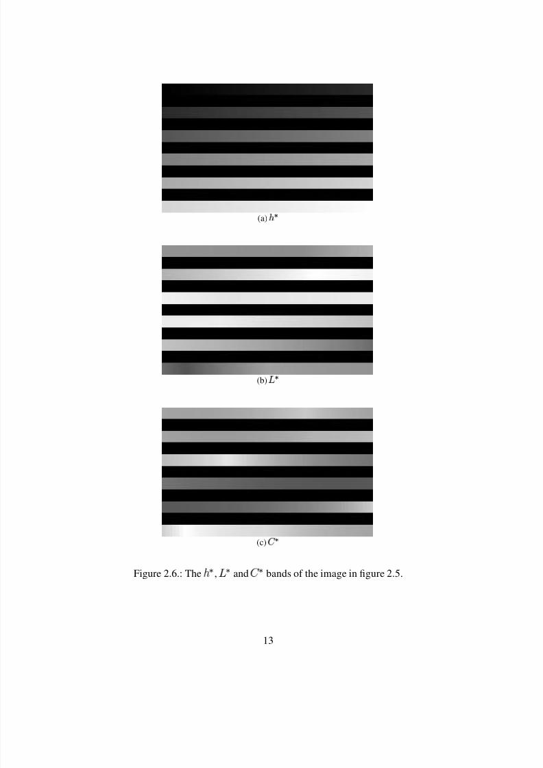
8/13/2019 Mathematical Morphology in the Lab Colour Space
Figure 2.4.: The values of the extrema of the chroma
and their corresponding luminance
as a function of hue
in the L*a*b* space.
corresponding to each integer value of
, along with the luminance
of the extremal point.
These functions are henceforth denoted as
and
, where the values can be read off
the graph for integer values of
, and interpolated for non-integer values.
2.5. Comparison between the HLS and L*a*b* spaces
In the HLS (double-cone) space, the points with highest saturation (
) have luminance
values of half the maximum (
). It is interesting to examine the relation between these
points and the extremal chroma points in the L*a*b* colour gamut. For the case we are treating,where use is made of primaries and a white point well adapted to computer monitors, the extrema
of the two spaces should coincide.
The extremal chroma points of the L*a*b* colour gamut are those plotted in figure 2.4, and
the colours corresponding to these points for integer hues between
and
are shown in
11
8/13/2019 Mathematical Morphology in the Lab Colour Space
numerical order of , so that one can order the points
and
where
. One can, for example, use cascades of lexicographical orders,
possibly dependent on the values of . In this new completely ordered lattice, the function is
replaced by a composite function , bi-unique, which permits one to assign a triplet
to a supremum or infimum of
.
3.2. The weighting function
In this section, we develop a weighting function allowing the colour vectors to be ordered, as
discussed in section 3.1. The weighting function associates a weight
with each colour
It is defined so that a lower weight implies a colour closer to the extremal points (more highly
saturated), and a higher weight indicates a colour close to the luminance axis (less saturated).
Four possible methods of defining weighting functions are discussed. The three methods
based on distance functions are rejected for reasons discussed in section 3.2.1, whereas the bestweighting function was found to be one modelled on an electrostatic potential, the details of
which are given in section 3.2.2.
3.2.1. Distance methods
Three possible methods were considered and rejected. The first is to measure the distance from
a colour in the L*a*b* space to the extremal point with the same hue. In symbolic form, the
weighting
of each colour point
is calculated as
(3.2)
where
and
are the extremal points (section 2.4.2). However, this approach does
not work as the L*a*b* colour gamut is not spherical. A two-dimensional illustration of this
problem is shown in figure 3.1. The extremal points of a simple two-dimensional non-circular
space with centre are shown. Using a two-dimensional version of equation 3.2, point would
be assigned a weight
equal to the distance , the distance to the extremal point with the same
hue. However, the distance to the closest extremal point is actually . This form of weighting
function therefore assigns too high a weight to some colours.
The second distance-based approach attempts to overcome the previous limitation by setting
the weight as the distance to the closest extremal point, or
(3.3)
With this formulation, however, we are hindered by the fact that the luminance axis is not in the
geometrical centre of the space. The grey colours are therefore not at an equal distance from the
17
8/13/2019 Mathematical Morphology in the Lab Colour Space
The weight (equation 3.6) is calculated for each colour vector in the L*a*b* space. A weight
image corresponding to a colour image is produced by replacing each colour pixel with its cor-
responding weight. The two weight images corresponding to figures 3.6a and b are shown in
figures 3.6c and d, where the grey-level represents the weight of the colour vector, and hence
darker pixels indicate colours which are closer to the extremal points.With the potential function approach, we have created a lattice of equipotential surfaces. The
colour vectors making up an equipotential surface have not yet been ordered. Unfortunately, the
best order for the colour vectors in the same equipotential surface is not obvious. In order to
obtain a complete ordering of the colour vectors, we make use of the lexicographical order. The
order of the equipotential surfaces is placed in the first level, followed by an arbitrary ordering
of the vectors in the same equipotential surface in the second and lower levels.
The following lexicographical orders for vectors
and
are introduced
(3.7)
and
(3.8)
where
is the hue origin chosen by the user, and
(3.9)
These two extra levels in the order relation are sufficient to completely order the colour vectors
as long as there are no spherical equipotential surfaces contained in the colour gamut. If use is
made of a charge configuration resulting in a spherically shaped equipotential surface included
in the colour gamut, then a fourth level relation for
would be necessary to retain the complete
ordering.
In a practical application of a morphological operator, the value of
is not critical, as it is
very seldom used, a phenomenon discussed further in section 3.5.
Note that the use of equation 3.9 does not directly result in a complete order, as is explained
in the following example. Two points
and
, where
is an arbitrary angle, have the same distances from the origin, even though they are not the
same point. We can impose a complete order by stating, for example, that in the situation where
and
, we take
if
, else
.
25
8/13/2019 Mathematical Morphology in the Lab Colour Space
Once these orders have been defined, the morphological operators are defined in the standard
way. The vector erosion at point
by structuring element
is
(3.10)
and the corresponding dilation by structuring element
is
(3.11)
An opening
is an erosion followed by a dilation, and a closing
is a dilation followed by
an erosion.
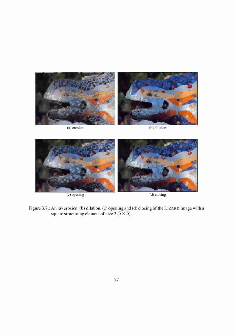
3.3.3. Examples
The first example demonstrates the behaviour of these operators. The L IZARD image was pur-
posely chosen as it contains highly coloured regions — the mosaic tiles — separated by greylines. The result of the erosion, dilation, opening and closing operators are shown in figure 3.7.
The operators produce the expected results, with the dilation operator enlarging the tiles, and the
erosion operator enlarging the regions between the tiles.
The second set of examples in figures 3.8 and 3.9 serve to illustrate the similarities and
differences between the approach presented for images in the L*a*b* space, and the analogous
approach in the HLS space of the lexicographical order with saturation in the first position [6].
The MIRO image used in the example is more demanding than the LIZARD image as it contains
black and white regions in addition to the coloured regions.
The results of the two approaches are strikingly similar, with the colours always being chosen
in preference to the black, white and grey pixels for the dilation operator. The main differences
are found when pixels of similar grey level or colours of similar saturation are ordered. Theeffects of the operators near the image borders have not been standardised, so the results in these
regions should be ignored.
3.4. Top-hat
One can create an operator analogous to the greyscale top-hat [12] for use on image in the L*a*b*
space. The greyscale opening top-hat is defined as
for all points
in
, and the greyscale closing top-hat is defined as
26
8/13/2019 Mathematical Morphology in the Lab Colour Space
The first two levels of this relation are obviously independent of the choice of the hue origin
. The hue only enters into the third level relation, and given the results of section 3.5, one
may be tempted to ignore this parameter as in practice it has little or no effect on the outcome of
the morphological operators. On the other hand, if we consider the complete ordering of all the
vectors in the HLS space, it is clear that the resulting order depends critically on the value of
.
The lexicographical order suggested for the L*a*b* space is similar to the above HLS space
order, and also consists of two levels which are rotationally invariant, and a third level depending
on the hue. These levels can be summarised as:
Order of equipotential surfaces (rotationally invariant).
Order of the luminance within each equipotential surface (rotationally invariant). This levelis in fact the order of a set of one-dimensional rings tracing out lines of equal potential and equal
luminance.
Order by hue within each equipotential equi-luminance ring (depends on the choice of a hue
origin).
In conclusion, the approach adopted in this report is to make the morphological operators
as “rotationally invariant as possible”. We do this by placing the relations which depend on the
choice of an origin in positions which have been experimentally shown to be almost never used,
so that in practice, their effect is almost negligible.
An alternative approach would be to start with operators which are designed to be rotationally
invariant on the hue, such as those introduced in [7], and add ways for them to take the othervector components into account. This remains to be explored.
33
8/13/2019 Mathematical Morphology in the Lab Colour Space
The use of a weighting function to impose an order on colours in the L*a*b* space is presented.
After introducing the theory underlying the use of a weighting function in the context of a vector
space, the electrostatic potential model is used as a basis for creating a weighting function which
simulates an order by colour saturation in the L*a*b* space. The weighting function has the
advantages of taking the positions of the luminance axis and extremal colours into account, and
being adaptable to many L*a*b* colour gamuts. The development of such a weighting function
is useful in that it avoids the necessity to transform to another colour space, an action possibly
accompanied by loss of colour information, before applying morphological operators based onan order by saturation. This is well demonstrated by the top-hat example, where we initially
ignore the inherent characteristics of the L*a*b* space by imposing an order based on colour
saturation, and then make intensive use of the perceptual uniformity characteristics during the
subtraction step.
The adaptation of the weighting function to other colour gamuts can be done by following
the steps presented in this report. One begins with the transformation of an RGB colour cube
completely filled with points to the L*a*b* space, after which the position of the extremal points
of the resultant colour gamut are found. The negative charges are placed at these extremal points,
and, not forgetting to take the positive charge on the luminance axis into account, the weight of
each colour can be determined.
The way in which the charge distribution at the extremal points is modelled should be im-proved. At the moment, the irregularly-shaped curve on which the extremal points are found is
approximated by a line of point charges. A formulation allowing these charges to be represented
as a continuous line charge, as for the line at the centre, will improve the results for highly satu-
rated colours. The calculation time of the weighting function is not critical, as the weight of each
colour only has to be calculated once for each colour gamut, after which a three-dimensional
look-up table can be used. An accurate implementation of the weighting function calculation
should therefore be possible.
This improvement in the accuracy of the weight calculation is necessary before this formu-
lation can be used for morphological reconstruction operators. With the current approximation
of the negatively charged line by relatively widely spaced point charges, some fully saturated
colours have lower weights than others, and one can therefore have an “invasion” of an image by
certain colours during a reconstruction process.
A possible useful modification to this technique could be to change the potential function
by adding charges elsewhere in the space. For example, if one is interested in regions of a
specific colour, an additional negative point charge could be placed at the position of this colour
34
8/13/2019 Mathematical Morphology in the Lab Colour Space
The transformation from the RGB to the L*a*b* space requires a passage through the XYZ
space. It is during the transformation from RGB to XYZ that the characteristics of the image
capture or display device and the illumination conditions are taken into account. A derivation of
the transformation from the RGB to XYZ colour space is given in section A.1, and shows how
any set of primaries and white point can be taken into account. For people pressed for time, a
matrix for transforming from RGB to XYZ for a set of commonly used primaries and white point
is given in section A.2. The other necessary transformations are XYZ to L*a*b* (section A.3)
and the inverse transformations, L*a*b* to XYZ (section A.4) and XYZ to RGB (section A.5).The material in this appendix is mainly from Poynton [11] and Wyszecki and Stiles [16].
A.1. RGB to XYZ derivation
A.1.1. Primaries and white point
We are working in a tristimulus RGB space with primary stimuli
so that an arbitrary stimulus is written as
where
,
and
are called the tristimulus values.
In colourimetric practice, a two-dimensional representation is often used, in which the coor-
dinates of the colours in the plane
are given. These chromaticity coordinates are
defined as
36
8/13/2019 Mathematical Morphology in the Lab Colour Space