Mathematical problems of General Relativity Lecture 2 Juan A. Valiente Kroon School of Mathematical Sciences Queen Mary, University of London [email protected], LTCC Course LMS Juan A. Valiente Kroon (QMUL) Mathematical GR 1 / 40
Transcript
Mathematical problems of General RelativityLecture 2
Juan A. Valiente Kroon
School of Mathematical SciencesQueen Mary, University of London
1 The 3 + 1 decomposition of General RelativitySubmanifolds of spacetimeFoliations of spacetimeThe intrinsic metric of an hypersurfaceThe extrinsic curvature of an hypersurfaceThe Gauss-Codazzi and Codazzi-Mainardi equationsThe constraint equations of General RelativityThe ADM-evolution equations
Juan A. Valiente Kroon (QMUL) Mathematical GR 2 / 40
The 3 + 1 decomposition of General Relativity Submanifolds of spacetime
Outline
1 The 3 + 1 decomposition of General RelativitySubmanifolds of spacetimeFoliations of spacetimeThe intrinsic metric of an hypersurfaceThe extrinsic curvature of an hypersurfaceThe Gauss-Codazzi and Codazzi-Mainardi equationsThe constraint equations of General RelativityThe ADM-evolution equations
Juan A. Valiente Kroon (QMUL) Mathematical GR 3 / 40
The 3 + 1 decomposition of General Relativity Submanifolds of spacetime
Submanifolds
Intuitive definition:
A submanifold of M, is a set N ⊂M which inherits a manifold structurefrom M.
Embeddings:
An embedding map ϕ : N →M which is injective and structure preserving;
The restriction ϕ : N → ϕ(N ) is a diffeomorphism.
Rigoruous definition of submanifold:
In terms of the above concepts, a submanifold N is the image ϕ(N ) ⊂M ofa k-dimensional manifold (k < n).
Very often it is convenient to identify N with ϕ(N ).
In what follows we will mosty be concerned with 3-dimensional submanifolds.It is customary to call these hypersurfaces.
Juan A. Valiente Kroon (QMUL) Mathematical GR 4 / 40
The 3 + 1 decomposition of General Relativity Foliations of spacetime
Outline
1 The 3 + 1 decomposition of General RelativitySubmanifolds of spacetimeFoliations of spacetimeThe intrinsic metric of an hypersurfaceThe extrinsic curvature of an hypersurfaceThe Gauss-Codazzi and Codazzi-Mainardi equationsThe constraint equations of General RelativityThe ADM-evolution equations
Juan A. Valiente Kroon (QMUL) Mathematical GR 5 / 40
The 3 + 1 decomposition of General Relativity Foliations of spacetime
Foliations
Globally hyperbolic spacetimes:
In what follows, we assume that the spacetime (M, gab) is globallyhyperbolic.
That is, we assume that its topology is that of R× S, where S is anorientable 3-dimensional manifold.
Globaly hyperbolic spacetimes are the natural class of spacetimes on which toformulate a Cauchy problem.
Definition of a foliation:
A spacetime is said to be foliated by (non-intersecting) hypersurfaces St,t ∈ R if
M =⋃t∈RSt,
where we identify the leaves St with {t} × S.
It is customary to think of the hypersurface S0 as an initial hypersurface onwhich the initial information giving rise to the spacetime is to be prescribed.
Juan A. Valiente Kroon (QMUL) Mathematical GR 6 / 40
The 3 + 1 decomposition of General Relativity Foliations of spacetime
Time functions
Definition:
In what follows it will be convenient to assume that the hypersurfaces Starise as the level surfaces of of a scalar function t which will be interpreted asa global time function.
From t one can define the the covector
ωa = ∇at.
By construction ωa denotes the normal to the leaves St of the foliation.
The covector ωa is closed —that is,
∇[aωb] = ∇[a∇b]t = 0.
Juan A. Valiente Kroon (QMUL) Mathematical GR 7 / 40
The 3 + 1 decomposition of General Relativity Foliations of spacetime
The lapse function
Definition:
Fom ωa one defines a scalar α called the lapse function via
gab∇at∇bt = ∇at∇at ≡ −1/α2.
The lapse measures how much proper time elapses between neighbouringtime slices along the direction given by the normal vector ωa ≡ gabωb.Assume that α > 0 so that ωa. Notice that ωa is assumed to be timelike sothat the hypersurfaces St are spacelike.
Unit normal:
In what follows we define the unit normal na via
na ≡ −αωa.The minus sign in the last definition is chosen so that na points in thedirection of increasing t.
One can readily verify that nana = −1.
One thinks of na as the 4-velocity of a normal observer whose worldline isalways orthogonal to the hypersurfaces St.
Juan A. Valiente Kroon (QMUL) Mathematical GR 8 / 40
The 3 + 1 decomposition of General Relativity The intrinsic metric of an hypersurface
Outline
1 The 3 + 1 decomposition of General RelativitySubmanifolds of spacetimeFoliations of spacetimeThe intrinsic metric of an hypersurfaceThe extrinsic curvature of an hypersurfaceThe Gauss-Codazzi and Codazzi-Mainardi equationsThe constraint equations of General RelativityThe ADM-evolution equations
Juan A. Valiente Kroon (QMUL) Mathematical GR 9 / 40
The 3 + 1 decomposition of General Relativity The intrinsic metric of an hypersurface
The intrinsic metric (I)
Definition:
The spacetime metric gab induces a 3-dimensional Riemannian metric hij onSt.The relation between gab and hab is given by
hab ≡ gab + nanb.
In the previous formula we regard the 3-metric as an object living onspacetime.
Properties:
The tensor hab is purely spatial —i.e. it has no component along na.
Contracting with the normal:
nahab = nagab + nananb = nb − nb = 0,
The inverse 3-metric hab is obtained by raising indices with
hab = gab + nanb
Juan A. Valiente Kroon (QMUL) Mathematical GR 10 / 40
The 3 + 1 decomposition of General Relativity The intrinsic metric of an hypersurface
The intrinsic metric (II)
Use as a projector:
The 3-metric hab can be used to project all geometric objects along thedirection given by na.
Effectively, hab decomposes tensors into a purely spatial part which lies onthe hypersurfaces St and a timelike part normal to the hypersurface.
In actual computations it is convenient to consider
hab = δa
b + nanb.
Given a tensor Tab its spatial part, to be denoted by T⊥ab is defined to be
T⊥ab ≡ hachbdTcd.
Juan A. Valiente Kroon (QMUL) Mathematical GR 11 / 40
The 3 + 1 decomposition of General Relativity The intrinsic metric of an hypersurface
The normal projector
Definition:
One can also define a normal projector Nab as
Nab ≡ −nanb = δa
b − hab.
In terms of these operators an arbitrary projector can be decomposed as
va = δabvb = (ha
b +Nab) = v⊥a − nanbvb.
Juan A. Valiente Kroon (QMUL) Mathematical GR 12 / 40
The 3 + 1 decomposition of General Relativity The intrinsic metric of an hypersurface
Covariant derivatives on hypersurfaces (I)
A definition of a covariant drivative:
The 3-metric hij defines in a unique manner a covariant derivative Di —theLevi-Civita connection of hij .
Work from a 4-dimensional (spacetime) perspective so that we write Da.
One requires Da to be torsion-free and compatible with the metric hab.
For a scalar φDaφ ≡ hab∇bφ,
and, say, for a (1, 1) tensor
DaTbc ≡ hadhebhcf∇dT ef ,
with an obvious extension to other tensors.
In coordinates, the covariant derivative Da is associated to the spatialChristoffel symbols
γµνλ = 12h
µρ(∂νhρλ + ∂λhνρ − ∂ρhνλ).
Juan A. Valiente Kroon (QMUL) Mathematical GR 13 / 40
The 3 + 1 decomposition of General Relativity The intrinsic metric of an hypersurface
Covariant derivatives on hypersurfaces (II)
The curvature of Da:
Being a covariant derivative, one can naturally associate a curvature tensorrabcd to Da by considering its commutator:
DaDbvc −DbDav
c = rcdabvd
One can verify that rcdabnd = 0.
Similarly, one can define the Ricci tensors and scalar as
rdb ≡ rcdcb, r ≡ gabrab.
Juan A. Valiente Kroon (QMUL) Mathematical GR 14 / 40
The 3 + 1 decomposition of General Relativity The extrinsic curvature of an hypersurface
Outline
1 The 3 + 1 decomposition of General RelativitySubmanifolds of spacetimeFoliations of spacetimeThe intrinsic metric of an hypersurfaceThe extrinsic curvature of an hypersurfaceThe Gauss-Codazzi and Codazzi-Mainardi equationsThe constraint equations of General RelativityThe ADM-evolution equations
Juan A. Valiente Kroon (QMUL) Mathematical GR 15 / 40
The 3 + 1 decomposition of General Relativity The extrinsic curvature of an hypersurface
The extrinsic curvature (I)
Motivation:
The Einstein field equation Rab = 0 imposes some conditions on the4-dimensional Riemann tensor Rabcd.
In order to understand the implications of the Einstein equations on anhypersurface one needs to decompose Rabcd into spatial parts. Thisdecomposition naturally involves rabcd.
The tensor rabcd measures the intrinsic curvature of the hypersurface St.This tensor provides no information about how St fits in (M, gab).
The missing information is contained in the so-called extrinsic curvature.
Juan A. Valiente Kroon (QMUL) Mathematical GR 16 / 40
The 3 + 1 decomposition of General Relativity The extrinsic curvature of an hypersurface
The extrinsic curvature (II)
Definition:
The extrinsic curvature is defined as the following projection of the spacetimecovariant derivative of the normal to St:
Kab ≡ −hachbd∇(cnd) = −hachbd∇cnd.
The second equality follows from the fact that na is rotation free.
By construction the extrinsic curvature is symmetric and purely spatial.
It measures how the normal to the hypersurface changes from point to point.
It also measures the rate at which the hypersurface deforms as it is carriedalong the normal —Ricci identity.
Juan A. Valiente Kroon (QMUL) Mathematical GR 17 / 40
The 3 + 1 decomposition of General Relativity The extrinsic curvature of an hypersurface
The acceleration
Definition:
The acceleration of a foliation is define via
aa ≡ nb∇bna.
Using nd∇c∇d = 0, one can compute
Kab = −hachbd∇cnd= −(δac + nan
c)(δbd + nbn
d)
= −(δac + nanc)δb
d∇cnd= −∇anb − naab.
Juan A. Valiente Kroon (QMUL) Mathematical GR 18 / 40
The 3 + 1 decomposition of General Relativity The extrinsic curvature of an hypersurface
An alternative expression for the extrinsic curvature
The Lie derivative of the intrinsic metric:
One computes
Lnhab = Ln(gab + nanb)
= 2∇(anb) + naLnnb + nbLnna= 2(∇(anb) + n(aab))
= −2Kab.
Juan A. Valiente Kroon (QMUL) Mathematical GR 19 / 40
The 3 + 1 decomposition of General Relativity The extrinsic curvature of an hypersurface
Mean curvature
Definition:
A related object is the so-called mean curvature:
K ≡ gabKab = habKab.
One can compute (exercise):
K = −Ln(ln deth).
Thus the mean curvature measures the fractional change in 3-dimensionalvolume along the normal na.
An hypersuface for which K = 0 everywhere is called maximal —it enclosesmaximum volume for a given area.
Juan A. Valiente Kroon (QMUL) Mathematical GR 20 / 40
The 3 + 1 decomposition of General Relativity The Gauss-Codazzi and Codazzi-Mainardi equations
Outline
1 The 3 + 1 decomposition of General RelativitySubmanifolds of spacetimeFoliations of spacetimeThe intrinsic metric of an hypersurfaceThe extrinsic curvature of an hypersurfaceThe Gauss-Codazzi and Codazzi-Mainardi equationsThe constraint equations of General RelativityThe ADM-evolution equations
Juan A. Valiente Kroon (QMUL) Mathematical GR 21 / 40
The 3 + 1 decomposition of General Relativity The Gauss-Codazzi and Codazzi-Mainardi equations
The Gauss-Codazzi equation
Motivation:
Given the extrinsic curvature of an hypersurface St, we now look how thisrelates to the curvature of spacetime.
A computation using the definitions of the previous section shows that
DaDbvc = ha
phbqhr
c∇p∇qvr −Kabhrcnp∇pvr −Ka
cKbpvp.
Combining with the commutator
DaDbvc −DbDav
c = rcdabvd,
after some manipulations one obtains
rabcd +KacKbd −KadKcb = haphb
qhcrhd
sRpqrs.
This equation is called the Gauss-Codazzi equation. It relates the spatialprojection of the spacetime curvature tensor to the 3-dimensional curvature.
Juan A. Valiente Kroon (QMUL) Mathematical GR 22 / 40
The 3 + 1 decomposition of General Relativity The Gauss-Codazzi and Codazzi-Mainardi equations
The Codazzi-Mainardi equation
Motivation:
A further important identity arises from considering projections of Rabcdalong the normal direction. This involves a spatial derivative of the extrinsiccurvature.
One has thatDaKbc = ha
phbqhc
r∇pKqr.
From this expression after some manipulations one can deduce
DbKac −DaKbc = haphb
qhcrnsRpqrs.
This equation is called the Codazzi-Mainardi equation.
In the sequel:
In the sequel, we explore the consequences of the Gauss-Codazzi andCodazzi-Mainardi equations for the initial value problem in General Relativity.
These give rise to the so-called constraint equations of General Relativity.
Juan A. Valiente Kroon (QMUL) Mathematical GR 23 / 40
The 3 + 1 decomposition of General Relativity The constraint equations of General Relativity
Outline
1 The 3 + 1 decomposition of General RelativitySubmanifolds of spacetimeFoliations of spacetimeThe intrinsic metric of an hypersurfaceThe extrinsic curvature of an hypersurfaceThe Gauss-Codazzi and Codazzi-Mainardi equationsThe constraint equations of General RelativityThe ADM-evolution equations
Juan A. Valiente Kroon (QMUL) Mathematical GR 24 / 40
The 3 + 1 decomposition of General Relativity The constraint equations of General Relativity
The constraint equations
Strategy:
The 3 + 1 decomposition of the Einstein field equations allows to identify theintrinsic metric and the extrinsic curvature of an initial hypersurface S0 as theinitial data to be prescribed for the evolution equations of General Relativity.
In what follows we will make use of the Gauss-Codazzi and theCodazzi-Mainardi equations to extract the consequences of the vacuumEinstein field equations
Rab = 0
on a hypersurface S.
Juan A. Valiente Kroon (QMUL) Mathematical GR 25 / 40
The 3 + 1 decomposition of General Relativity The constraint equations of General Relativity
The Hamiltonian constraint (I)
Derivation of the equation:
Contracting the Gauss-Codazzi equation one finds that
hprhbqhd
sRpqrs = rbd +KKbd −KcdKcb,
where K ≡ habKab denotes the trace of the extrinsic curvature.
A further contraction then yields
hprhqsRpqrs = r +K2 −KabKab.
Now, the left-hand side can be expanded into
hprhqsRpqrs = (gpr + npns)(gqs + nqns)
= R+ 2npnrRpr + npnrnqnsRpqrs = 0.
The last term vanishes beacuse of the symmetries of the Riemann tensor.
Juan A. Valiente Kroon (QMUL) Mathematical GR 26 / 40
The 3 + 1 decomposition of General Relativity The constraint equations of General Relativity
The Hamiltonian constraint (II)
Summarising
Combining the equations from the previous calculations one obtains the so-calledHamiltonian constraint:
r +K2 −KabKab = 0.
Juan A. Valiente Kroon (QMUL) Mathematical GR 27 / 40
The 3 + 1 decomposition of General Relativity The constraint equations of General Relativity
The momentum constraint
Derivation:
Contracting once the Codazzi-Mainardi equation one has that
DbKab −DaK = haphqrnsRpqrs.
The right hand side of this equation can be, in turn, expanded as
haphqrnsRpqrs = −hap(gqr + npnr)nsRqprs
= −hapnsRps − hapnqnrnsRpqrs = 0,
where in the last equatlity one makes use, again, of the vacuum Equationsand the symmetries of the Riemann tensor.
Summarising:
Combining the previous expressions one obtains the so-called momentumconstraint:
DbKab −DaK = 0.
Juan A. Valiente Kroon (QMUL) Mathematical GR 28 / 40
The 3 + 1 decomposition of General Relativity The constraint equations of General Relativity
Initial data and the constraint equations
Discussion:
The Hamiltonian and momentum constraint involve only the 3-dimensionalintrinsic metric, the extrinsic curvature and their spatial derivatives.
They are the conditions that allow a 3-dimensional slice with data (hab,Kab)to be embedded in a 4-dimensional spacetime (M, gab).
The existence of the constraint equations implies that the data for theEinstein field equations cannot be prescribed freely.
Remark:
An important point still to be clarified is the sense in which the fields hab and Kab
correspond to data for the Einstein field equations. To see this, one has to analysethe evolution equations implied by the Einstein field equations.
Juan A. Valiente Kroon (QMUL) Mathematical GR 29 / 40
The 3 + 1 decomposition of General Relativity The constraint equations of General Relativity
The constraint equations for the electromagnetic field (I)
A source of insight:
The equations of other physical theories also imply constraint equations. Theclassical example in this respect is given by the Maxwell equations.
In order to analyse the constraint equations implied by the Maxwell equationsit is convenient to introduce the electric and magnetic parts of the Faradaytensor Fab:
Ea ≡ Fabnb, Ba ≡ 12εab
cdFcdnb = F ∗abn
b.
A calculation then shows that the Maxwell equations imply the constraintequations
DaEa = 0, DaBa = 0.
These constraints correspond to the well-known Gauss laws for the electricand magnetic fields.
Juan A. Valiente Kroon (QMUL) Mathematical GR 30 / 40
The 3 + 1 decomposition of General Relativity The constraint equations of General Relativity
The constraint equations for the electromagnetic field (II)
Summarising:
Thus, it follows that data for the Maxwell equations cannot be prescribedfreely. The initial value of the electric and magnetic parts of the Faradaytensor must be divergence free.
Notice, by contrast that the wave equation for a scalar field φ implies noconstraint equations. Thus, the data for this equation can be prescribedfreely.
Juan A. Valiente Kroon (QMUL) Mathematical GR 31 / 40
The 3 + 1 decomposition of General Relativity The ADM-evolution equations
Outline
1 The 3 + 1 decomposition of General RelativitySubmanifolds of spacetimeFoliations of spacetimeThe intrinsic metric of an hypersurfaceThe extrinsic curvature of an hypersurfaceThe Gauss-Codazzi and Codazzi-Mainardi equationsThe constraint equations of General RelativityThe ADM-evolution equations
Juan A. Valiente Kroon (QMUL) Mathematical GR 32 / 40
The 3 + 1 decomposition of General Relativity The ADM-evolution equations
The Ricci equation
Strategy:
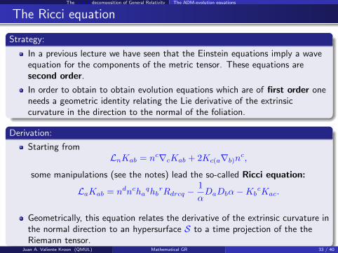
In a previous lecture we have seen that the Einstein equations imply a waveequation for the components of the metric tensor. These equations aresecond order.
In order to obtain to obtain evolution equations which are of first order oneneeds a geometric identity relating the Lie derivative of the extrinsiccurvature in the direction to the normal of the foliation.
Derivation:
Starting fromLnKab = nc∇cKab + 2Kc(a∇b)nc,
some manipulations (see the notes) lead the so-called Ricci equation:
LaKab = ndnchaqhb
rRdrcq −1
αDaDbα−Kb
cKac.
Geometrically, this equation relates the derivative of the extrinsic curvature inthe normal direction to an hypersurface S to a time projection of the theRiemann tensor.
Juan A. Valiente Kroon (QMUL) Mathematical GR 33 / 40
The 3 + 1 decomposition of General Relativity The ADM-evolution equations
The Ricci equation
Strategy:
In a previous lecture we have seen that the Einstein equations imply a waveequation for the components of the metric tensor. These equations aresecond order.
In order to obtain to obtain evolution equations which are of first order oneneeds a geometric identity relating the Lie derivative of the extrinsiccurvature in the direction to the normal of the foliation.
Derivation:
Starting fromLnKab = nc∇cKab + 2Kc(a∇b)nc,
some manipulations (see the notes) lead the so-called Ricci equation:
LaKab = ndnchaqhb
rRdrcq −1
αDaDbα−Kb
cKac.
Geometrically, this equation relates the derivative of the extrinsic curvature inthe normal direction to an hypersurface S to a time projection of the theRiemann tensor.
Juan A. Valiente Kroon (QMUL) Mathematical GR 33 / 40
The 3 + 1 decomposition of General Relativity The ADM-evolution equations
The time vector and the shift vector (I)
The time vector:
The discussion from the previous paragraphs suggests that the Einstein fieldequations will imply an evolution of the data (hab,Kab).
Assumed that the spacetime (M, gab) is foliated by a time function t whoselevel surfaces corresponds to the leaves of the foliation.
Recalling that ωa = ∇at, we consider now a vector ta (the time vector)such that
ta = αna + βa, βana = 0.
Juan A. Valiente Kroon (QMUL) Mathematical GR 34 / 40
The 3 + 1 decomposition of General Relativity The ADM-evolution equations
The time vector and the shift vector (II)
The shift vector:
The vector βa is called the shift vector.
The time vector ta will be used to propagate coordinates from one timeslice to another.
In other words, ta connects points with the same spatial coordinate —hence,the shift vector measures the amount by which the spatial coordinates areshifted within a slice with respect to the normal vector.
Juan A. Valiente Kroon (QMUL) Mathematical GR 35 / 40
The 3 + 1 decomposition of General Relativity The ADM-evolution equations
The time vector and the shift vector (III)
Gauge functions:
Together, the lapse and shift determine how coordinates evolve in time. Thechoice of these functions is fairly arbitrary and hence they are known asgauge functions.
The lapse function reflects the to choose the sequence of time slices, pushingthem forward by different amounts of proper time at different spatial pointson a slice —this idea is usually known as the many-fingered nature of time.
The shift vector reflects the freedom to relabel spatial coordinates on eachslices in an arbitrary way.
Observers at rest relative to the slices follow the normal congreunce na andare called Eulerian observers, while observers following the congruence ta
are called coordinate observers.
It is observed that as a consequence of the previous definitions one has thatta∇at = 1 so that the integral curves of ta are naturally parametrised by t.
Juan A. Valiente Kroon (QMUL) Mathematical GR 36 / 40
The 3 + 1 decomposition of General Relativity The ADM-evolution equations
The evolution equation for the 3-metric
Derivation of the equation:
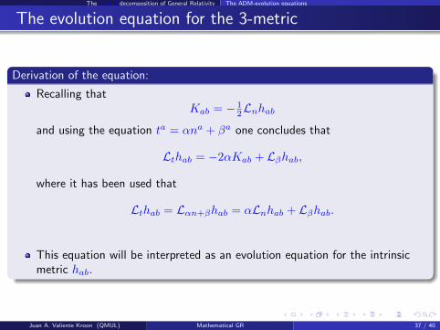
Recalling thatKab = − 1
2Lnhaband using the equation ta = αna + βa one concludes that
Lthab = −2αKab + Lβhab,
where it has been used that
Lthab = Lαn+βhab = αLnhab + Lβhab.
This equation will be interpreted as an evolution equation for the intrinsicmetric hab.
Juan A. Valiente Kroon (QMUL) Mathematical GR 37 / 40
The 3 + 1 decomposition of General Relativity The ADM-evolution equations
Evolution equation for the second fundamental form
Derivation of the equation:
In order to construct a similar equation for the extrinsic curvature one makesuse of the Ricci equation.
It is noticed that
ndnchaqhb
rRdrcq = hcdhaqhb
rRdrcq − haqhbrRrq= hcdha
qhbrRdrcq,
where to obtain the second equality Rab = 0 has been used. The remainingterm, hcdha
qhbrRdrcq is dealt with using the Gauss-Codazzi equation.
Finally, noticing that
LtKab = Lαn+βKab = αLnKab + LβKab,
one concludes that
LtKab = −DaDbα+ α(rab − 2KacKcb +KKab) + LβKab.
This is the desired evolution equation for Kab.
Juan A. Valiente Kroon (QMUL) Mathematical GR 38 / 40
The 3 + 1 decomposition of General Relativity The ADM-evolution equations
The 3+1 equations and the Einstein field equations
Remarks:
The evolution equations deduced in the previous slices determine theevolution of the data (hab,Kab). These equations are usually known as theADM (Arnowitz-Deser-Misner) equations.
Together with the constraint equations they are completely equivalent tothe vacuum Einstein field equations.
The ADM evolution equations are first order equations —contrast with thewave equation for the components of the metric gab discussed in a previouslecture. However, the equations are not hyperbolic!
Thus, one cannot apply directly the standard PDE theory to assert existenceof solutions. Nevertheless, there are some more complicated versions whichdo have the hyperbolicity property.
Juan A. Valiente Kroon (QMUL) Mathematical GR 39 / 40
The 3 + 1 decomposition of General Relativity The ADM-evolution equations
The Maxwell evolution equations
A source of insight:
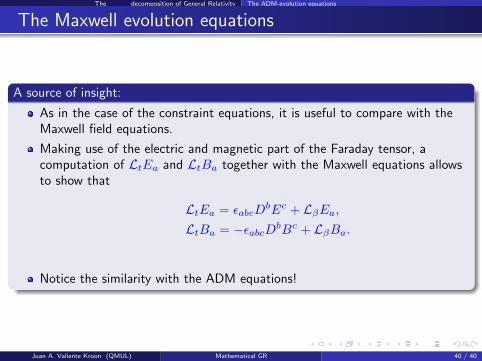
As in the case of the constraint equations, it is useful to compare with theMaxwell field equations.
Making use of the electric and magnetic part of the Faraday tensor, acomputation of LtEa and LtBa together with the Maxwell equations allowsto show that
LtEa = εabcDbEc + LβEa,
LtBa = −εabcDbBc + LβBa.
Notice the similarity with the ADM equations!
Juan A. Valiente Kroon (QMUL) Mathematical GR 40 / 40