Mathematical statistics in physics and astronomy Radu Stoica Universit´ e Lille - Laboratoire Paul Painlev´ e Observatoire de Paris - Institut de M´ ecanique C´ eleste et Calcul d Eph´ em´ erides [email protected]Tartu, September, 2014
Transcript
Mathematical statistics in physics and astronomy
Radu StoicaUniversite Lille - Laboratoire Paul Painleve
Observatoire de Paris - Institut de Mecanique Celeste et Calculd Ephemerides
24 hours = 4 weeks × 6 hours = 4 weeks × 2 days times 3hours
mark : project + written/oral exam (last day of the course -you need a mark of 50% to validate it)
Bibliogaphical references
• Baddeley, A. J. (2010) Analysing spatial point patterns in ’R’.Workshop Notes, Version 4.1.• Diggle, P. J. (2003) Statistical analysis of spatial point patterns.Arnold Publishers.• van Lieshout, M. N. M. (2000) Markov point processes and theirapplications. Imperial College Press.• Martinez, V. J., Saar, E. (2002) Statistics of the galaxydistribution. Chapman and Hall.• Møller, J., Waagepetersen, R. P. (2004) Statistical inference andsimulation for spatial point processes. Chapman and Hall/CRC.V• Chiu, S. N., Stoyan, D., Kendall, W. S., Mecke, J. (2013)Stochastic geometry and its applications. John Wiley and Sons.
Aknowledgements
A. J. Baddeley, G. Castellan, J.-F. Coeurjolly, X. Descombes, P.Gregori, C. Lantuejoul, M. N. M. van Liehsout, V. Martinez, J.Mateu, J. Møller, Z. Pawlas, F. Rodriguez, E. Saar, D. Stoyan, E.Tempel, R. Waagepetersen, J. Zerubia
Lesson IIntroductionSome data sets and their related questions
Lesson IIMathematical backgroundDefinition of a point processBinomial point processPoisson point process
Lesson IIIMoment and factorial moment measures, product densitiesMore properties of the Poisson processCampbell moment measuresCampbell - Mecke formula
Lesson IVInterior and exterior conditionningA review of the Palm theorySlivnyak - Mecke theoremApplications : summary statistics
Lesson V
Reduced Palm distributionsCampbell and Slivnyak theoremsSummary statistics : the K and L functionsExterior conditioning : conditional intensity
Lesson VIIProbability density of a point processesInteracting marked point processesMarkov point processes
Lesson VIIIMonte Carlo simulationMarkov chains : a little bit of theoryMetropolis-Hastings algorithmMH algorithm for sampling marked point processesSpatial birth-and-death processes
Perfect or exact simulation
Lesson IXStatistical inference problemsMonte Carlo Maximum likelihood estimationParameter estimation based on pseudo-likelihoodModel validation : residual analysis for point processesStatistical pattern detection
Conclusion and perspectives
What is this course about ?
Spatial data analysis : investigate and describe data sets whoseelements have two components
position : spatial coordinates of the elements in a certainspace
characteristic : value(s) of the measure(s) done at thisspecific location
what is the data subset made of those elements having acertain ”common” property ?
”The” answer :
generally, this ”common” property may be described by astatistical analysis
the spatial coordinates of the spatial data elements add amorphological component to the answer
the data subset we are looking for, it forms a pattern that hasrelevant geometrical characteristics
”The” question re-formulated :
what is the pattern hidden in the data ?
what are the geometrical and the statistical characteristics ofthis pattern ?
Aim of the course : provide you with some mathematical tools toallow you formulate answers to these questions
Examples : data sets and related questions
For the purpose of this course : software and data sets areavailable
R library : spatstat by A. Baddeley, R. Turner andcontributors → www.spatstat.org
C++ library : MPPLIB by A. G. Steenbeek, M. N. M. vanLieshout, R. S. Stoica and contributors → available at simpledemand
Toravere Observatory : huge quantities of data sets and software,and the questions going together with
there are plenty of future Nobel subjects for you :)
contact : E. Tempel, L. J. Liivamagi, E. Saar and myself
Forestry data (1) : the points positions exhibit attraction →clustered distribution
redwoodfull
Figure: Redwoodfull data from the spatstat package
> library(spatstat)
> data(redwoodfull) ; plot(redwoodfull)
Forestry data (2) : the points positions exhibit neither attractionnor repulsion → completely random distribution
japanesepines
Figure: Japanese data from the spatstat package
In order to see all the available data sets> data(package="spatstat")
Biological data (1) : the points positions exhibit repulsion →regular distribution
cells
Figure: Cell data from the spatstat package
> data(cells)
> cells
planar point pattern: 42 points
window: rectangle = [0, 1] x [0, 1] units
Biological data (2) : two types of cells exhibiting attraction andrepulsion depending on their relative positions and types
amacrine
Figure: Amacrine data from the spatstat package
> data(amacrine) ;
plot(amacrine,cols=c("blue","red"))
Animal epidemiology : sub-clinical mastitis for diary herds
points → farms location
to each farm → disease score (continuous variable)
clusters pattern detection : regions where there is a lack ofhygiene or rigour in farm management
0 50 100 150 200 250 300 3500
50
100
150
200
250
300
Figure: The spatial distribution of the farms outlines almost the entireFrench territory (INRA Avignon).
Cluster pattern : some comments
particularity of the disease : can spread from animal to animalbut not from farm to farm
cluster pattern : several groups (regions) of points that areclose together and have the “same statistical properties”
clusters regions → approximate it using interacting smallregions (random disks)
local properties of the cluster pattern : small regions wherelocally there are a lot of farms with a high disease score value
problem : pre-visualisation is difficult ...
Image analysis : road and hydrographic networks
a) b)
Figure: a) Rural region in Malaysia (http://southport.jpl.nasa.gov), b)Forest galleries (BRGM).
Thin networks : some comments
road and hydrographic networks → approximate it byconnected random segments
topologies : roads are “straight” while rivers are “curved”
texture : locally homogeneous, different from its right and itsleft with respect a local orientation
avoid false alarms : small fields, buildings,etc.
local properties of the network : connected segments coveredby a homogeneous texture
Geological data : two types of patterns, line segments and points→ are these patterns independent ?
Copper
Figure: Copper data from the spatstat package
> attach(copper) ; L=rotate(Lines,pi/2) ;
P=rotate(Points,pi/2)
> plot(L,main="Copper",col="blue") ;
points(P$x,P$y,col="red")
Cosmology (1) : spatial distribution of galactic filaments
Figure: Cuboidal sample from the North Galactic Cap of the 2dF GalaxyRedshift Survey. Diameter of a galaxy ∼ 30× 3261.6 light years.
Cosmology (2) : study of mock catalogs
a) b)
Figure: Galaxy distribution : a) Homogeneous region from the 2dfNcatalog, b) A mock catalogue within the same volume
Cosmology (3) : questions and observations
Real data
filaments, walls and clusters : different size and contrast
inhomogeneity effects (only the brightest galaxies areobserved)
filamentary network the most relevant feature
local properties of the filamentary network : connectingrandom cylinders containing a “lot” of galaxies “along” itsmain axis ...
Mock catalogues
how “filamentary” they are w.r.t the real observation ?
how the theoretical models producing the synthetic data fitsthe reality ?
Oort cloud comets (1)
The comets dynamics :
comets parameters (z , q, cos i , ω,Ω) → inverse of thesemi-major axis,perihelion distance, inclination, perihelionargument, longitude of the ascending node
variations of the orbital parameters
initial state : parameters before entering the planetary regionof our Solar System
final state : current state
question : do these perturbation exhibit any spatial pattern ?
Oort cloud comets (2)
Study of the planetary perturbations
∼ 107 perturbations were simulated
data → set of triplets (q, cos i ,z)
spatial data framework : location (q, cos i) and marks z
z = zf − zi :perturbations of the cometary orbital energy
local properties of the perturbations : locations are uniformlyspread in the observation domain, marks tend to be importantwhenever they are close to big planets orbits
reformulated question : do these planetary observationsexhibit an observable spatial pattern ?
problem : pre-visualisation is very difficult ...
Spatio-temporal data (1)
Time dimension available :
the previous example may be considered snapshots
more recent data sets have also a temporal coordinate
question : what is the pattern hidden in the data and itstemporal behaviour ?
Satellite debris :
after explosion, the debris of two colliding artificial satellitesdistributes a long an orbit around Earth
test the uniformity of the debris along the orbit
characterize the spatio-temporal distribution of the entire setof debris
extremely interesting set : the evolution of the objectsdynamics is known from the initial state, i.e. no debris at all
→ video spatial debris
Spatio-temporal data (2)
Roads dynamics in Central Africa region :
in forest region with rare woods, road networks appear anddisappear within the territory of an exploitation concession
there is a difference between “classical” road networks and“exploitation” networks → mining galleries
this roads dynamics may be relevant in many aspects : healthof the forest, respect of rules for the enterprises,environmental behaviour and understanding
characterize the distribution and the dynamics of the roadnetwork
→ video roads dynamics
Synthesis
Hypothesis : the pattern we are looking for can be approximatedby a configuration of random objects that interact
marked points pattern : repulsive or attractive marked points
clusters pattern : superposing random disks
filamentary network : connected and aligned segments
Important remark :
locally : the number of objects is finite
Marked point processes :
probabilistic models for random points with randomcharacteristics
origin → stochastic geometry
the pattern is described by means of a probability density →stochastic modelling
the probability density allows the computation of averagequantities and descriptors (these are integrals) related to thepattern
Remarks :
there exist also deterministic mathematical tools able to treatpattern recognition problems
probability is cool : the phenomenon is not controlled, butunderstood
probability thinking framework offers simultaneously theanalysis and the synthesis abilities of the proposed method
probabilistic approach deeply linked with physics →exploratory analysis, model formulation, simulation, inference
comets example : random fields → another probabilisticmathematical tool
unifying random fields and marked point processes is amathematical challenge
spatio - temporal example : requires new clean andappropriate mathematics, based on both stochastic processesand stochastic geometry
still, partial answers to these questions can be given using thetools presented in this course
present challenge : big data
Lesson IIntroductionSome data sets and their related questions
Lesson IIMathematical backgroundDefinition of a point processBinomial point processPoisson point process
Lesson IIIMoment and factorial moment measures, product densitiesMore properties of the Poisson processCampbell moment measuresCampbell - Mecke formula
Lesson IVInterior and exterior conditionningA review of the Palm theorySlivnyak - Mecke theoremApplications : summary statistics
Lesson V
Reduced Palm distributionsCampbell and Slivnyak theoremsSummary statistics : the K and L functionsExterior conditioning : conditional intensity
Lesson VIIProbability density of a point processesInteracting marked point processesMarkov point processes
Lesson VIIIMonte Carlo simulationMarkov chains : a little bit of theoryMetropolis-Hastings algorithmMH algorithm for sampling marked point processesSpatial birth-and-death processes
Perfect or exact simulation
Lesson IXStatistical inference problemsMonte Carlo Maximum likelihood estimationParameter estimation based on pseudo-likelihoodModel validation : residual analysis for point processesStatistical pattern detection
Conclusion and perspectives
Measure and integration theory → blackboard
σ−algebra
measurable space, sets, functions
measure
measure space, integral with respect to a measure
probability space, probability measure
Construction of a point processes
Mathematical ingredients :
observation window : the measure space (W ,B, ν), withW ⊂ R
d , B the Borel σ−algebra and 0 < ν(W ) <∞ theLebesgue measure
points configuration space : probability space (Ω,F ,P)Configuration space construction :
state space Ω :
Wn is the set of all n-tuples w1, . . . ,wn ⊂ WΩ = ∪∞
n=0Wn, n ∈ N
events space F : the σ− algebra given by
F = σ(w = w1, . . . ,wn ∈ Ω : n(wB) = n(w ∩ B) = m)
with B ∈ B and m ∈ N
probability measure P : the model answering our questions
DefinitionA point process in W is a measurable mapping from a probabilityspace (S,A) in (Ω,F). Its distribution is given by
P(X ∈ F ) = Pω ∈ S : X (ω) ∈ F,
with F ∈ F . The realization of a point process is random set ofpoints in W . We shall sometimes identify X and P(X ∈ F ) andcall them both a point process.
Remarks : point process ⇒ random configuration of points w in aobservation window W
a points configuration is w = w1,w2, . . . ,wn, with n thecorresponding number of points
locally finite : n(w) is finite whenever the volume of W isfinite
simple : wi 6= wj for i 6= j
in this course, W is almost always a compact set ...
from time to time we will consider also the case W = Rd but
this should not worry you ... too much ...
→ drawing
Marked point processes : attach characteristics to the points →extra-ingredient : marks probability space (M,M, νM)
DefinitionA marked point process is a random sequence x = xn = (wn,mn)such that the points wn are a point process in W and mn are themarks corresponding for each wn.
Examples :
random circles : M = (0,∞)
random segments : M = (0,∞)× [0, π]
multi-type process : M = 1, 2, . . . , k... and all the possible combinations ... → drawing
Stationarity and isotropy. A point process X on W is stationary ifit has the same distribution as the translated proces Xw , that is
w1, . . . ,wn L= w1 + w , . . . ,wn + w
for any w ∈ W .A point process X on W is isotropic if it has the same distributionas the rotated proces rX , that is
w1, . . . ,wn L= rw1, . . . , rwn
for any rotation matrix r.
motion invariant : stationary and isotropic
marked case : in principle easy to generalize, but take care ...
Intuitive description of a point process : being able to say howmany points of the process X can be found in any neighbourhoodof WThe mathematical tools for point processes : should be able to dothe following
count the points of a point process in a small neighbourhoodof a point in W , and then extend the neighbourhood
count the points of a point process in a small neighbourhoodof a typical point of the process X , and then extend theneighbourhood
counting within this context means using a probabilitymeasure based counter
Let X be a point process on W , and let us consider the countingvariable
N(B) = n(XB), B ∈ B,representing the number of points “falling” in B .Let us consider also the sets of the form
FB = x ∈ Ω : n(xB) = 0,
that are called void events.
DefinitionThe distribution of a point process X is determined by the finitedimensional distributions of its count function, i.e. the jointdistribution of N(B1), . . . ,N(Bm) for any B1, . . . ,Bm ∈ B andm ∈ N.
TheoremThe distribution of a point process is uniquely determined by itsvoid probabilities
v(B) = P(N(B) = 0), B ∈ B.
Remarks :
the previous definition is sometimes considered amathematical result ...
the proof of the theorem shows first, that the events set Fcan be built using the void set made of FB ’s. Then, ameasure theory argument says that two measures acting in thesame way on a first original event set, they will act similarlyon a second event set generated from the previous one
this result is easy to generalize for marked point processes,but with care ...
the generalization of the previous result can be done also withrespect to W : complete and separable (Polish) space
Binomial point process
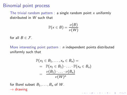
The trivial random pattern : a single random point x uniformlydistributed in W such that
P(x ∈ B) =ν(B)
ν(W )
for all B ∈ F .
More interesting point pattern : n independent points distributeduniformly such that
P(x1 ∈ B1, . . . , xn ∈ Bn) =
= P(x1 ∈ B1) · . . . · P(xn ∈ Bn)
=ν(B1) · . . . · ν(Bn)
ν(W )n
for Borel subset B1, . . . ,Bn of W .→ drawing
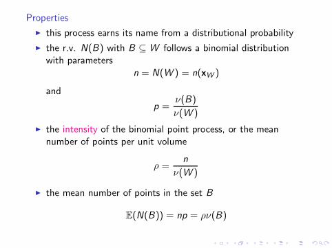
Properties
this process earns its name from a distributional probability
the r.v. N(B) with B ⊆ W follows a binomial distributionwith parameters
n = N(W ) = n(xW )
and
p =ν(B)
ν(W )
the intensity of the binomial point process, or the meannumber of points per unit volume
ρ =n
ν(W )
the mean number of points in the set B
E(N(B)) = np = ρν(B)
the binomial process is simple : all points are isolated
number of points in different subsets of W are notindependent even if the subsets are disjoint
N(B) = m ⇒ N(W \ B) = n−m
the distribution of the point process is characterized by thefinite dimensional distributions
P(N(B1) = n1, . . . ,N(Bk) = nk) for k = 1, 2, . . .
such that n1 + n2 + . . .+ nk ≤ n
if the Bk are disjoint Borel sets with B1 ∪ . . .Bk = W andn1 + . . .+ nk = n, the finite-dimensional distributions aregiven by the multinomial probabilities
P(N(B1) = n1, . . . ,N(Bk) = nk)
=n!
n1! . . . nk !
ν(B1)n1 . . . ν(Bk)
nk
ν(W )n
the void probabilities for the binomial point process are givenby
v(B) = P(N(B) = 0) =(ν(W )− ν(B))n
ν(W )n
Stationary Poisson point process
Motivation :
convergence binomial towards Poisson
→ drawing + blackboard
Definition : a stationary (homogeneous) Poisson point process X ischaracterized by the following fundamental properties
Poisson distribution of points counts. The random number ofpoints of X in a bounded Borel set B has a Poissondistribution with mean ρν(B) for some constant ρ, that is
P(N(B) = m) =(ρν(B))m
m!exp(−ρν(B))
Independent scattering. The number of points of X in kdisjoint Borel sets form k independent random variables, forarbitrary k
Properties
simplicity : no duplicate points
the mean number of points in a Borel set B is
E(N(B)) = ρν(B)
ρ : the intensity or density of the Poisson process, and itrepresents the mean number of points in a set of unit volume
0 < ρ <∞, since for ρ = 0 ⇒ the process contains no points,while for ρ = ∞ we get a pathological case
if B1, . . . ,Bk are disjoint Borel sets, then N(B1), . . . ,N(Bk)are independent Poisson variable with meansρν(B1), . . . , ρν(Bk).Thus
P(N(B1) = n1, . . . ,N(Bk) = nk)
=ρn1+...+nkν(B1)
n1 . . . ν(Bk)nk
n1! · . . . · nk !exp
(−
k∑
i=1
ρν(Bi)
),
this formula can be used to compute joint probabilities foroverlapping sets
the void probabilities for the Poisson point process are givenby
v(B) = P(N(B) = 0) = exp(−ρ(ν(B)))
the Poisson point process with ρ = ct. is stationary andisotropic
if the intensity is a function ρ : W → R+ such that
∫
B
ρ(w)dν(w) <∞
for bounded subsets B ⊆ W , then we have a inhomogeneousPoisson process with mean
E(N(B)) =
∫
B
ρ(w)dν(w) = Υ(B)
Υ is called the intensity measure
we have already seen that for the stationary Poisson process :Υ(B) = ρν(B)
Mapping theorem
a Poisson process on W mapped into another space W ′ by afunction ψ is still a Poisson process, provided ψ is measurableand has no atoms
ψ has no atoms ↔ ψ does not map several points from Winto a single point in W ′
consequence : the projection of a Poisson process is also aPoisson process
if ψ is a linear transformation, then we have :
TheoremLinear transformation of a Poisson process. Let A : Rd → R
d anon-singular mapping. If X is a stationary Poisson process ofintensity ρ, then AX = Aw : w ∈ X is also a stationary Poissonprocess and its intensity is ρ|det(A−1)|, where det(A−1) is thedeterminant of the inverse of A.
Spherical contact distribution :
F (r) = P(d(w ,X ) < r)
= 1− P(d(w ,X ) > r)
= 1− P(b(w , r) ∩ X = ∅)
with b(w , r) the ball centred in w ∈ W and with radius r . Forthe stationary Poisson point processes on W ⊂ R
2, we get
F (r) = 1− P(N(b(o, r)) = 0) = 1− exp(−ρπr2)
Remark : the spherical contact distribution does not completelycharacterize a point process, because it is obtained for a particularset B
Conditioning and binomial point processes. Let X be astationary Poisson point process on W a compact set in R
d ,and consider the conditioning N(W ) = n. The resultingprocess is a binomial point process with n points.
This is easily verified, by computing the void probabilities in acompact subset B ⊂ W → Exercice 1 and 2
a Poisson point process on Rd is obtained by adding
“disjoint” boxes till covering the whole domain ...
The most important marked Poisson point proces : the unitintensity Poisson point process with i.i.d. marks on a compact W
number of objects ∼ Poisson(ν(W ))
locations and marks i.i.d. : wi ∼ 1ν(W ) and mi ∼ νM
The corresponding probability measure : weighted ‘counting” ofobjects
P(X ∈ F ) =∞∑
n=0
e−ν(W )
n!
∫
W×M
· · ·∫
W×M
1F(w1,m1), . . . , (wn,mn)
×dν(w1)dνM(m1) . . . dν(wn)dνM(m)
for all F ∈ F .Remark : the simulation of this process is straightforward, whilethe knowledge of the probability distribution allows analyticalcomputations of the interest quantities
Simulations results of some Poissonian point processes : thedomain is W = [0, 1]× [0, 1] and the intensity parameter is ρ = 100
a)
Poisson point process
b)
Multi−type Poisson point process
c)
Poisson segment process
0.00 0.25 0.50 0.75 1.00
Figure: Poisson based models realizations : a) unmarked, b) multi-typeand c) Boolean model of segments.
→ Exercice 3
Some general facts concerning the binomial and the Poisson pointprocesses
the law is completely known → analytical formulas,
independence → no interaction → no structure in the data ...
completely random patterns : null or the default hypothesisthat we want to reject
more complicate models can be built → specifying aprobability density p(x) w.r.t. the reference measure given bythe unit intensity Poisson point process. This probabilitymeasure is written as
P(X ∈ F ) =
∫
F
p(x)µ(dx)
with µ the reference measure.
Remark : in this case the normalizing constant is not availablefrom an analytical point of view. To check this replace in theexpression of µ(·) the indicator function 1Fy with p(y) ...
Lesson IIntroductionSome data sets and their related questions
Lesson IIMathematical backgroundDefinition of a point processBinomial point processPoisson point process
Lesson IIIMoment and factorial moment measures, product densitiesMore properties of the Poisson processCampbell moment measuresCampbell - Mecke formula
Lesson IVInterior and exterior conditionningA review of the Palm theorySlivnyak - Mecke theoremApplications : summary statistics
Lesson V
Reduced Palm distributionsCampbell and Slivnyak theoremsSummary statistics : the K and L functionsExterior conditioning : conditional intensity
Lesson VIIProbability density of a point processesInteracting marked point processesMarkov point processes
Lesson VIIIMonte Carlo simulationMarkov chains : a little bit of theoryMetropolis-Hastings algorithmMH algorithm for sampling marked point processesSpatial birth-and-death processes
Perfect or exact simulation
Lesson IXStatistical inference problemsMonte Carlo Maximum likelihood estimationParameter estimation based on pseudo-likelihoodModel validation : residual analysis for point processesStatistical pattern detection
Conclusion and perspectives
Moment and factorial moment measures, product densities
Present context :
mathematical background
definition of a marked point process
Binomial and Poisson point process
important result : the point process law is determined bycounts of points
Let X be a point process on W . The counts of points in Borelregions of B ⊂ W , N(B) characterize the point process and theyare well defined random variables
it is difficult to average the pattern X
it is possible to compute moments of the N(B)’s
The appropriate mathematical tools are :
the moment measures
the factorial moment measures
the product densities
→ blackboard
More properties of the Poisson process
Stationary Poisson point processes : compute the momentmeasures, the factorial moment measures and the product densities
find relations between all these for this process
→ Exercice 4
DefinitionA disjoint union ∪∞
i=1Xi of point processes X1,X2, . . . is calledsuperposition.
Proposition
If Xi ∼ Poissson(W , ρi) , i = 1, 2, . . . are mutually independentand if ρ =
∑ρi is locally integrable, then with probability one,
X = ∪∞i=1Xi is a disjoint union and est X ∼ Poisson(W , ρ) .
→ stable character of the Poisson process
DefinitionLet be q : W → [0, 1] a function and X a point process on W .The point process Xthin ⊂ X obtained by including the ξ ∈ X inXthin with probability q(ξ), where points are included/excludedindependently of each other, is said to be an independent thinningof X with retention probabilities q(ξ).
Formally, we can set
Xthin = ξ ∈ X : R(ξ) ≤ q(ξ),
with the random variables R(ξ) ∼ U [0, 1], ξ ∈ W , mutuallyindependent and independent of X .
Proposition
Suppose that X ∼ Poisson(W , ρ) is subject to independentthinning with retention probabilities q(ξ), ξ ∈ W and let
ρthin = q(ξ)ρ(ξ), ξ ∈ W .
Then Xthin and X \ Xthin are independent Poisson processes withintensity functions ρthin and ρ− ρthin, respectively.
Corollary
Suppose that X ∼ Poisson(W , ρ) with ρ bounded by a positiveconstant C. Then X is distributed as independent thinning of aPoisson(W ,C ) with retention probabilities q(ξ) = ρ(ξ)/C.
Remarks : utility of the previous results
the Poisson process is invariant under independent thinning
easy procedure for simulate non-stationary Poisson process
the n−th product density measure of an independentlythinned point process is
ρ(n)thin(w1, . . . ,wn) = ρ(n)(w1, . . . ,wn)
n∏
i=1
q(wi )
this gives the invariance under independent thinning of then−th point correlation function (van Lieshout, 2011)
ρ(n)thin(w1, . . . ,wn)
ρthin(w1) · . . . · ρthin(wn)=
ρ(n)(w1, . . . ,wn)
ρ(w1) · . . . · ρ(wn)
but watch out ...
→ Exercice 5 : explain the envelope tests
Campbell moment measures
Present context :
counting points i.e. computing moment and factorial momentmeasures → very interesting tool for analysing pointpatterns : allow the computation of average quantities
still, compute an average pattern → difficult and challengingproblem
idea : counting points that have some specific properties →Campbell measures
DefinitionLet X be a point process on W . The Campbell measure is
C (B × F ) = E [N(B)1X ∈ F] ,
for all B ∈ B and F ∈ F .
The first order moment measure can be expressed as a Campbellmeasure :
C (B ×Ω) = E[N(B)] = µ(1)(B).
Higher order Campbell measures are constructed in a similarmanner. For instance, the second ordre Campbell measure is
C (2)(B1 × B2 × F ) = E [N(B1)N(B2)1X ∈ F] ,
from which we can get the second order moment measure
C (2)(B1 × B2 ×Ω) = E [N(B1)N(B2)] = µ(2)(B1 × B2)
Remark :
the moment measures allow to average functions h(x)measured in the location of a point process X : the function hdoes not depend on X
the Campbell measures allow to average functions h(x , x)measured in the location of a point process X : the function hmay depend on X
Campbell - Mecke formula
TheoremLet h : W × Ω → [0,∞) a measurable function that is eithernon-negative either integrable with respect to the Campbellmeasure. Then
E
[∑
w∈X
h(w ,X )
]=
∫
W
∫
Ωh(w , x)dC (w , x).
Proof.→ blackboard
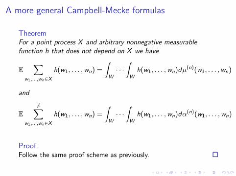
A more general Campbell-Mecke formulas
TheoremFor a point process X and arbitrary nonnegative measurablefunction h that does not depend on X we have
E
∑
w1,...,wn∈X
h(w1, . . . ,wn) =
∫
W
· · ·∫
W
h(w1, . . . ,wn)dµ(n)(w1, . . . ,wn)
and
E
6=∑
w1,...,wn∈X
h(w1, . . . ,wn) =
∫
W
· · ·∫
W
h(w1, . . . ,wn)dα(n)(w1, . . . ,wn)
Proof.Follow the same proof scheme as previously.
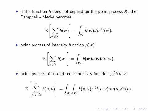
If the function h does not depend on the point process X , theCampbell - Mecke becomes
E
[∑
w∈X
h(w)
]=
∫
W
h(w)dµ(1)(w).
point process of intensity function ρ(w)
E
[∑
w∈X
h(w)
]=
∫
W
h(w)ρ(w)dν(w).
point process of second order intensity function ρ(2)(u, v)
E
6=∑
u,v∈X
h(u, v)
=
∫
W
∫
W
h(u, v)ρ(2)(u, v)dν(u)dν(v).
Lesson IIntroductionSome data sets and their related questions
Lesson IIMathematical backgroundDefinition of a point processBinomial point processPoisson point process
Lesson IIIMoment and factorial moment measures, product densitiesMore properties of the Poisson processCampbell moment measuresCampbell - Mecke formula
Lesson IVInterior and exterior conditionningA review of the Palm theorySlivnyak - Mecke theoremApplications : summary statistics
Lesson V
Reduced Palm distributionsCampbell and Slivnyak theoremsSummary statistics : the K and L functionsExterior conditioning : conditional intensity
Lesson VIIProbability density of a point processesInteracting marked point processesMarkov point processes
Lesson VIIIMonte Carlo simulationMarkov chains : a little bit of theoryMetropolis-Hastings algorithmMH algorithm for sampling marked point processesSpatial birth-and-death processes
Perfect or exact simulation
Lesson IXStatistical inference problemsMonte Carlo Maximum likelihood estimationParameter estimation based on pseudo-likelihoodModel validation : residual analysis for point processesStatistical pattern detection
Conclusion and perspectives
Interior and exterior conditioning
Present context :
counting points measures : count the points in a smallneighbourhood and then integrate using the Campbell Meckeformula → the small neighbourhood is a small region in W
idea : the “same” counting points measures → the smallneighbourhood is a small region in W “centred” in a point ofthe process X → interior conditionning
question : how the measures applied to a process X change, ifwe add or if we delete a point from the current configuration→ exterior conditionning
A review of the Palm theory
construction → blackboard
the Palm distributions of X at w ∈ W can be interpreted as
Pw (F ) = P(X ∈ F |N(w) > 0)
the Campbell - Mecke formula can be expressed as
E
[∑
w∈X
h(w ,X )
]=
∫
W
∫
Ωh(w , x)dPw (x)dµ
(1)(w)
for stationary point processes
E
[∑
w∈X
h(w ,X )
]
= ρ
∫
W
∫
Ωh(w , x)dPw (x)dν(w)
= ρ
∫
W
∫
Ωh(w , x+ w)dPo(x)dν(w)
Slivnyak - Mecke theorem
TheoremIf X ∼ Poisson(W , ρ), then for functions g : W × Ω → [0,∞), wehave
E
∑
w∈X
h(w ,X \ w) =∫
W
Eh(w ,X )ρ(w)dν(w),
(where the left hand side is finite if and only if the right hand sideis finite).
proof : → blackboard
generalization : rather easy ... (the same comment as for theCampbell - Mecke theorem)
this theorem is a very strong result, since it allows computingaverages of a Poisson point process knowing that one orseveral points belong to the process ...
application in telecomunications : knowing, in this location Ihave a mobile phone antena, how the quality of the signalchange if I add randomly more antenas ? (the group of F.Baccelli)
combining the Campbell-Mecke and the Slivnyak-Mecketheorem, we obtain for a Poisson proces
∫
Ωh(x)dPw (x) =
∫
Ωh(x ∪ w)dP(x)
in words : the Palm distribution of a Poisson process withrespect to w is simply the Poisson distribution plus an addedpoint at w
a more mathematical formulation : the Palm distributionPΥw (·) of a Poisson process of intensity measure Υ and
distribution PΥ is the convolution P
Υ ⋆ δw of PΥ with anadditional deterministic point at w
explanation : blackboard
→ Exercice 6 and 7
Assumption : X is a stationary point process
the nearest neighbour distance distribution function
G (r) = Pw (d(w ,X \ w) ≤ r) (1)
with Pw the Palm distribution. The translation invariance ofthe distribution of X → inherited by the Palm distribution →G(r) is well-defined and does not depend on the choice of w .
replacing the Palm distribution in (1) by the distribution of X→ the spherical contact distribution or the empty spacefunction
F (r) = P(d(w ,X ) ≤ r)
with P the distribution of X .
the J function : compares nearest neighbour to emptydistances
J(r) =1− G (r)
1− F (r)
defined for all r > 0 such that F (r) < 1
The J function describes the morphology of a point pattern withrespect to a Poisson process :
For the stationary Poisson process of intensity parameter ρ, onW ⊂ R
2, these statistics have exact formulas :
F (r) = 1− exp[−ρπr2]G (r) = F (r)
J(r) = 1
→ Exercice 8
Lesson IIntroductionSome data sets and their related questions
Lesson IIMathematical backgroundDefinition of a point processBinomial point processPoisson point process
Lesson IIIMoment and factorial moment measures, product densitiesMore properties of the Poisson processCampbell moment measuresCampbell - Mecke formula
Lesson IVInterior and exterior conditionningA review of the Palm theorySlivnyak - Mecke theoremApplications : summary statistics
Lesson V
Reduced Palm distributionsCampbell and Slivnyak theoremsSummary statistics : the K and L functionsExterior conditioning : conditional intensity
Lesson VIIProbability density of a point processesInteracting marked point processesMarkov point processes
Lesson VIIIMonte Carlo simulationMarkov chains : a little bit of theoryMetropolis-Hastings algorithmMH algorithm for sampling marked point processesSpatial birth-and-death processes
Perfect or exact simulation
Lesson IXStatistical inference problemsMonte Carlo Maximum likelihood estimationParameter estimation based on pseudo-likelihoodModel validation : residual analysis for point processesStatistical pattern detection
Conclusion and perspectives
Reduced Palm distributions
Present context :
Palm distributions : count the points in a neighbourhoodcentred on a point of the process → this point is counted aswell
idea : in some applications (telecommunications) we may wishto measure the effect of a point process in a location being apoint of the process, while this particular point has no effecton the entire process → reduced Palm distributions
the following mathematical development is rather easy tofollows since it is similar to what we have already seen duringuntil now
Reduced Campbell measure
DefinitionLet X be a simple point process on the complete, separable metricspace (W , d). The reduced Campbell measure is
C !(B × F ) = E
[∑
w∈X∩B
1X \ w ∈ F],
for all B ∈ B and F ∈ F .
the analogue of Campbell-Mecke formula reads
E
[∑
w∈X
h(w ,X \ w)]=
∫
W
∫
Ωh(w , x)dC !(w , x).
assuming the first order moment measure µ(1) of X exists andit is σ−finite, we can apply Radon-Nikodym theory to write
C !(B × F ) =
∫
B
P !w (F )dµ
(1)(w),
for all B ∈ B and F ∈ F the function P !
· (F ) is defined uniquely up to an µ(1)−null set
it is possible to find a version such that for fixed w ∈ W ,P !w (·) is a probability distribution → the reduced Palm
distribution
Campbell and Slivnyak theorems
the reduced Palm distribution can be interpreted as theconditional distribution
P !w (F ) = P(X \ w ∈ F |N(w) > 0)
the Campbell-Mecke formula equivalent
E
[∑
w∈X
h(w ,X \ w)]=
∫
W
∫
Ωh(w , x)dP !
w (x)dµ(1)(w).
for stationary point processes
E
[∑
w∈X
h(w ,X \ w)]
= ρ
∫
W
∫
Ωh(w , x)dP !
w (x)dν(w)
= ρ
∫
W
∫
Ωh(w , x+ w)dP !
o(x)dν(w)
the Slivnyak-Mecke theorem : for a Poisson process on Wwith distribution P, we have
P !w (·) = P(·)
there is a general result linking the reduced Palm distributionand the distribution of a Gibbs process → a little bit later inthis course ...
Example
The nearest neighbour distribution G (r) of stationary process canbe expressed in terms of the Palm distributions
G (r) = 1− Po(X ∈ Ω : N(b(o, r)) = 1),
and the reduced Palm distributions
G (r) = 1− P !o(X ∈ Ω : N(b(o, r)) = 0),
where N(b(o, r)) is the number of points inside the ball centred atthe origin o of radius r .
Summary statistics : the K and L functions
The K function :
maybe one of the most used summary statistic
for a stationary process, its definition depending on thereduced Palm distribution is
ρK (r) = E!o [N(b(o, r))]
the L function is
L(r) =
[K (r)
ωd
]1/d
with ωd = ν(b(0, 1)) the volume of the d−dimensional unitball
for stationary point processes, the pair correlation function is
g(r) =K ′(r)
σd rd−1
with σd the surface area of the unit sphere in Rd
for the stationary Poisson process we have
K (r) = ωd rd , g(r) = 1
andL(r) = r
theoretical explanations → blackboard
Exterior conditioning : conditional intensity
assume that for any fixed bounded Borel set A ∈ B, thereduced Campbell measure C !(A× ·) is absolutely continuouswith respect to the distribution P(·) of X
then
C !(A × F ) =
∫
F
Λ(B ; x)dP(x)
for some measurable function Λ(B ; ·) specified uniquely up toa P−null set
moreover, one can find a version such that for fixed x, Λ(·; x)is a locally finite Borel measure → the first order Papangeloukernel
if Λ(·; x) admits a density λ(·; x) with respect to the Lebesguemeasure ν(·) on W , the Campbell-Mecke theorem becomes
E
[∑
w∈X
h(w ,X \ w)]
=
∫
W
∫
Ωh(w , x)dC !(w , x)
= E
[∫
W
h(w ,X )λ(w ;X )dν(w)
]
the function λ(·; ·) is called the Papangelou conditionalintensity
the previous result is known as the Georgii-Nguyen-Zessinformula
the case where the distribution of X is dominated by aPoisson process is especially important
TheoremLet X be a finite point process specified by a density p(x) withrespect to a Poisson process with non-atomic finite intensitymeasure ν. Then X has Papangelou conditional intensity
the infinitesimal probability of finding a point in a regiondν(u) around u ∈ W given that the point process agrees withthe configuration x outside of dν(u)
the “conditional reverse” of the Palm distributions
describe the local interactions in a point pattern → Markovpoint processes
ifλ(u; x) = λ(u; ∅)
for all patterns x satisfying x ∩ b(u, r) = ∅ → the process has‘interactions of range r at u’
in other words, points further than r away from u do notcontribute to the conditional intensity at u
integrability of the model
convergence of the Monte Carlo dynamics able to simulate themodel
differential characterization of Gibbs point processes →blackboard
→ Exercice 9
Lesson IIntroductionSome data sets and their related questions
Lesson IIMathematical backgroundDefinition of a point processBinomial point processPoisson point process
Lesson IIIMoment and factorial moment measures, product densitiesMore properties of the Poisson processCampbell moment measuresCampbell - Mecke formula
Lesson IVInterior and exterior conditionningA review of the Palm theorySlivnyak - Mecke theoremApplications : summary statistics
Lesson V
Reduced Palm distributionsCampbell and Slivnyak theoremsSummary statistics : the K and L functionsExterior conditioning : conditional intensity
Lesson VIIProbability density of a point processesInteracting marked point processesMarkov point processes
Lesson VIIIMonte Carlo simulationMarkov chains : a little bit of theoryMetropolis-Hastings algorithmMH algorithm for sampling marked point processesSpatial birth-and-death processes
Perfect or exact simulation
Lesson IXStatistical inference problemsMonte Carlo Maximum likelihood estimationParameter estimation based on pseudo-likelihoodModel validation : residual analysis for point processesStatistical pattern detection
Conclusion and perspectives
Some main ideas to be retained till now
counting measures → summary statistics for point patterncharacterization
two categories : interpoint distances (F ,G and J) and secondorder characteristics (ρ,K and L)
possible extension of the summary statistics : marks,non-stationary processes, different observation spaces W caseand spatio-temporal → some of these topics are alreadysolved, others are rather hot research topics
non-parametrical estimation of the summary statistics : kernelestimation and management of the border effects + numericalsensitivity → not presented in this course, but Enn and histeam are experts of this domain ...
central limit available : statistical tests
summary statistics for parameter estimation of the undergoingmodel ⇒ these statistics are an ”equivalent” of the momentsin probability theory, hence they do not entirely determine themodel to be estimated ... (Baddeley and Silverman, 1984)
good exploring tool : spatstat provides also some 3destimators ...
outline important aspects of a point pattern : clustering,repulsion, completely randomness
→ real need for models able to reproduce these characteristics→ counting is not always obvious ...
Cox processes
DefinitionLet Υ be a random locally finite diffuse measure on (W ,B). If theconditional distribution of X given Υ is a Poisson process on Wwith intensity measure Υ, X is said to be a Cox point process withdriving measure Υ. Sometimes X is also called doubly stochasticPoisson process.
Remarks :
if there exists a random field Z = Z (w),w ∈ W such that
Υ(B) =
∫
B
Z (w)dν(w)
then X is a Cox process with driving function Z
the conditional distribution of X given Z = z is a distributionof the Poisson process with intensity function z ⇒
E[N(B)|Z = z] =
∫
B
z(w)dν(w)
the first order factorial moment measure is obtained using thelaw of the total expectation
µ(1)(B) = α(1)(B) = E[N(B)]
= E [E[N(B)|Z = z]] = E
[∫
B
Z (w)dν(w)
]
= E[Υ(B)] =
∫
B
EZ (w)dν(w)
if ρ(w) = EZ (w) exists then it is the intensity function
smilarly, it can be shown that the second order factorialmoment measure is
α(2)(B1 × B2) = E [Υ(B1)Υ(B2)]
= E
[∫
B1
Z (u)dν(u)
∫
B2
Z (v)dν(v)
]
= E
[∫
B1
∫
B2
Z (u)Z (v)dν(u)dν(v)
]
=
∫
B1
∫
B2
E [Z (u)Z (v)] dν(u)dν(v)
if ρ(2)(u, v) = EZ (u)Z (v) exists, then it is the product density
proof : use the results from Exercice 4 and the totalexpectation law
the pair correlation function is
g(u, v) =ρ(2)(u, v)
ρ(u)ρ(v)=
E [Z (u)Z (v)]
E [Z (u)]E [Z (v)]
depending on Z it is possible to obtain analytical formulas forthe second order characteristics (g ,K and L) and theinterpoint distance characteristic (F ,G and J)
the variance VarN(B) is obtained using the total variance law,and it is
VarN(B) = EN(B) + Var
[∫
B
Z (w)dν(w)
]≥ EN(B)
⇒ over - dispersion of the Cox process counting variables
the void probabilities of Cox processes are
P(N(B) = 0)) = E1N(B) = 0= E [E1N(B) = 0|Z = z)] = E [P(N(B) = 0|Z = z)]
= E
[exp
(−∫
B
Z (w)dν(w)
)]
= E [exp (−Υ(B))]
Trivial Cox process : mixed Poisson processes
Z (w) = Z0 a common positive random variable for alllocations w ∈ W
X |Z0 follows a homogeneous Poisson process with intensity Z0
the driving measure is Υ(B) = Z0ν(B)
Thinning of Cox processes
X is a Cox process driven by Z
Π = Π(w) : w ∈ W ⊆ [0, 1] is a random field which isindependent of (X ,Z )
Xthin|Π → the point process obtained by independent thinningof the points in X with retention probabilities Π
⇒ Xthin is a Cox process driven by Zthin(w) = Π(w)Z (w)
Cluster processes
DefinitionLet C be a point process (parent process), and for each c ∈ C letXc be a finite point process (daughter process). Then
X =⋃
c∈C
Xc
is called a cluster point process.
DefinitionLet X be a cluster point process such that C is a Poisson pointprocess and conditional on C, the processes Xc , c ∈ C areindependent. Then X is called a Poisson cluster point process.
DefinitionLet X be a Poisson cluster point process such that centreddaughter processes Xc − c are independent of C . Given C, let thepoints of Xc − c be i.i.d. with density function k on R
d and N(Xc )be i.i.d. random variables. Then X is called a Neyman-Scottprocess. If moreover N(Xc ) given C has a Poisson distribution withintensity α, then X is a Neyman-Scott Poisson process.
→ drawing + Exercice 10
TheoremLet X be a Neyman-Scott Poisson process such that C is astationary Poisson process with intensity κ. Then X is stationaryprocess with intensity ρ = ακ and pair correlation function
g(u) = 1 +h(u)
κ,
where
h(u) =
∫k(v)k(u + v)dν(v)
is the density for the difference between two independent pointswhich have density k.
Proof.→ blackboard
Matern cluster process (Matern 1960,1986)
k(u) =1‖ u ‖≤ r
ωd rd
is the uniform density on the ball b(o, r)
Thomas process (Thomas 1949)
k(u) =exp
(−‖u‖2
2ω2
)
(2πω2)d/2
is the density for Nd (0, ω2Id ), i.e. for d independent normally
distributed variables with mean 0 and variance ω2 > 0
both kernels are isotropic
the Thomas process pair correlation function is
g(u) = 1 +1
κ(4πω2)d/2exp
[−‖ u ‖2
4ω2
]
and its K−function for d = 2 is
K (r) = πr2 +1− exp[−r2/(4ω2)]
κ
other summary statistics can be also computed
the expressions of the summary statistics are morecomplicated for the Matern process
→ drawing + show on your computer Exercice 11 + data sets(redwoodfull, japanesepines, celss)
Remarks :
usually in applications Z is unobserved
we cannot distinguish a Cox process X from its correspondingPoisson process X |Z when only one realisation of X isavailable
open question : which of the two models might be mostappropriate, i.e. whether Z should be random or“systematic”/deterministic
prior knowledge of the observed phenomenon
Bayesian setting of the intensity function ⇒ Cox processes
if we want to investigate the dependence of certain covariatesassociated to Z , these may be treated as systematic terms,while unobserved effects may be treated as random terms
Cox process : more flexible models for clustered patterns thaninhomogeneous Poisson point processes
Boolean model
Random objects “centred” around Poissonian points → germs andgrains
germs : a stationary Poisson point process X of intensity ρ onRd
grains : a sequence of i.i.d. random compact sets Γ1, Γ2, . . .and independent of X
The Boolean model is the random set obtained by the replacementof the germs by the appropriately shifted corresponding set, andtaking the set union as it follows
Γ =
∞⋃
n=1
(Γn + wn) = (Γ1 + w1) ∪ (Γ2 + w2) ∪ . . .
The random set Γ0 is said to be the typical grain. The set Γ is alsocalled the Poisson germ-grain model.
The Boolean model observation is an incomplete observation of amarked point process, since the locations points is not available
a)
Boolean model of random discs
b)
Boolean model : what is really observed
Figure: Boolean model of random discs : complete and incomplete views.
important practical applications → one of the first models ofcomplex patttern
no structure ↔ no objects interactions
Neyman-Scott processes may be seen as Boolean models aswell ...
Capacity functional.Choquet theorem
in general, for random sets it is rather difficult to use momentand factorial measures ↔ it is not possible to “count” points
un-marked and marked point processes are particular randomsets
DefinitionThe capacity functional the random closed set Γ is
TΓ(K ) = P(Γ ∩ K 6= ∅)
for K an element of the family K of compact sets in Rd .
Theorem(Choquet theorem). The distribution of a random closed set Γ iscompletely determined by the capacity functionals TΓ(K ) for allK ∈ K.
Capacity functional of the Boolean model
Proposition
The capacity functional of the Boolean model Γ is
TΓ(K ) = 1− exp[−ρE(ν(Γ0 ⊕ K ))
].
the reflection of the typical grain :
Γ0 = −Γ0 = −w : w ∈ A, for A ⊂ Rd
the Minkowski addition :
A⊕ B = u + v : u ∈ A, y ∈ B, for A,B ⊂ Rd
Proof.→ blackboard
Basic characteristics of the Boolean model
the volume fraction
covariance
contact distribution
→ blackboard
Stability of the Boolean model
Proposition
The following properties are satisfied :i) the union of two independent Boolean models is a Booleanmodelii) a Boolean model dilated by a non-empty compact subset of Rd
is a Boolean modeliii) the intersection between a Boolean model and a compactsubset of Rd is a Boolean modeliv) the cross-section of a Boolean model by an i-flat is a Booleanmodel
Proof.→ blackboard
Lesson IIntroductionSome data sets and their related questions
Lesson IIMathematical backgroundDefinition of a point processBinomial point processPoisson point process
Lesson IIIMoment and factorial moment measures, product densitiesMore properties of the Poisson processCampbell moment measuresCampbell - Mecke formula
Lesson IVInterior and exterior conditionningA review of the Palm theorySlivnyak - Mecke theoremApplications : summary statistics
Lesson V
Reduced Palm distributionsCampbell and Slivnyak theoremsSummary statistics : the K and L functionsExterior conditioning : conditional intensity
Lesson VIIProbability density of a point processesInteracting marked point processesMarkov point processes
Lesson VIIIMonte Carlo simulationMarkov chains : a little bit of theoryMetropolis-Hastings algorithmMH algorithm for sampling marked point processesSpatial birth-and-death processes
Perfect or exact simulation
Lesson IXStatistical inference problemsMonte Carlo Maximum likelihood estimationParameter estimation based on pseudo-likelihoodModel validation : residual analysis for point processesStatistical pattern detection
Conclusion and perspectives
Probability density of a point processes
Present context :
the independence property of the Poisson based processesdoes not allow to introduce point interactions
interactions can be introduced by means of a probabilitymeasure w.r.t a Poissonian reference measure µ
the distribution of such a point process writes as
P(X ∈ F ) =
∫
F
p(x)dµ(x)
let µ be the standard unit intensity Poisson process
the point process distribution w.r.t µ writes as
P(X ∈ F ) =
=∞∑
n=0
exp[−ν(W )]
n!
∫
W
· · ·∫
W
1(w1, . . . ,wn ∈ F )×
p(w1, . . . ,wn)dν(w1) . . . dν(wn),
whenever n > 0. If n = 0, we take exp[−ν(W )]1(∅ ∈ F )p(∅).If ν(W ) = 0, then P(X = ∅) = 1. For applications, we alwaysassume that ν(W ) > 0.
the marked case writes in a similar way by introducing alsothe marks distribution νM
usually the probability density is known up to a constant :p ∝ h
the normalizing constant or the partition function is given by
α =
∫
Ωh(x)dµ(x)
that becomes
α =∞∑
n=0
exp[−ν(W )]
n!
∫
W
· · ·∫
W
h(w1, . . . ,wn)dν(w1) . . . dν(wn)
(2)
the previous quantity is not always available under analyticalclosed form
this is the main difficulty to be solved while ausing thisapproach ...
Normalizing constant for the Poisson process : Let ρ be theintensity function of a Poisson point process on W . Its probabilitydensity up to a normalizing constant is
p(w) ∝∏
wi∈w
ρ(wi ).
Let Υ(B) =∫Bρ(w)dν(w) be the associated intensity measure.
We asssume 0 < Υ(B) <∞ for any B ⊆ W .By using (2), we get
α = exp[−ν(W )]
∞∑
n=0
Υ(W )n
n!= exp[Υ(W )− ν(W )],
that gives for the complete probability density
p(w) = exp[ν(W )−Υ(W )]∏
wi∈w
ρ(wi )
If the process is stationary ρ(w) = ρ = ct., then the probabilitydensity is
p(w) = exp[(1 − ρ)ν(W )]ρn
Interacting marked point processes
Construction of the probability density :
specify the interaction functions φ(k) : Ω → R+
φ(xi1 , . . . , xik )(k)
for any k−tuplet of objects
the density is the product of all these functions
p(x) = α∏
xi∈x
φ(xi )(1) · · ·
∏
xi1 ,...,xik ∈x
φ(xi1 , . . . , xik )(k) (3)
α the normalizing constant is not known
the probability densities (3) are suitable for modelling providedthey are integrable on Ω ; that is
α =
∫
Ωp(x)dµ(x) <∞.
the following results ensure the integrability of the probabilitydensity of a marked point process → the Ruelle stabilityconditions
DefinitionLet X be a marked point process with probability density p w.r.tthe reference measure µ. The process X is stable in the sense ofRuelle, if it exists Λ > 0 such that
p(x) ≤ Λn(x), ∀x ∈ Ω. (4)
Proposition
The probability density of a stable point process is integrable.
Proof.The integrability of p(x) follows directly from the precedingcondition :
∫
Ωp(x)µ(dx) ≤
∫
ΩΛn(x)µ(dx)
=∞∑
n=0
exp[−ν(W )][Λν(W )])n
n!= exp[ν(W )(Λ − 1)].
DefinitionUnder the same hypotheses as in Prop. 5, a marked point processis said to be locally stable if it exists Λ > 0 such that
p(x ∪ η) ≤ Λp(x), ∀x ∈ Ω, η ∈ W ×M \ x (5)
Proposition
A locally stable point process is stable in the sense of Ruelle.
Proof.It is easy to show by induction that
p(x) = p(∅)Λn(x), ∀x ∈ Ω.
The local stability of a point process (5) implies itsintegrability (4).
the local stability implies the hereditary condition
p(x) = 0 ⇒ p(y) = 0, if x ⊆ y.
this condition allows the definition of the conditional intensityas
λ(η; x) =p(x ∪ η)
p(x), x ∈ Ω, η ∈ W ×M \ x,
assuming 0/0 = 0
the conditional intensity is also known in the literature as thePapangelou intensity condition (we have already meet it)
Importance of the conditional intensity : key element in modelling
plays a similar role as the conditional probabilities for Markovrandom fields
integrability
convergence properties of the MCMC algorithms used tosample from p
the process X is attractive if x ⊆ y implies
λ(η; x) ≤ λ(η; y),
and repulsive otherwise
λ(η; x) ≥ λ(η; y),
attractive processes tend to cluster the points, while therepulsive ones tend to distance the points
these conditions are important also for exact MCMCalgorithms
there exist processes that are neither attractive nor repulsive
there are processes that are integrable but not locally stable :Lennard - Jones (statistical physics)
Markov point processes
The conditional intensity of an interacting point process is given by
λ(η; x) = φ(η)(1)∏
xi∈x
φ(xi , η)(2) · · ·
∏
xi1 ,...,xik ∈x
φ(xi1 . . . . , xik , η)(k+1)
difficult to manipulate
possible simplifications : limit the order of interactions → onlypairs of points for instance
limit the range of the interaction : a point interact only withits closest neighbours
Let ∼ be a symmetrical and reflexive relation between pointsbelonging to W ×M. This may be a typical neighbourhoodrelation based on a metric (Euclidean, Hausdorff) or on setsintersection.
DefinitionA clique is a configuration x ∈ Ω such that η ∼ ζ for all η, ζ ∈ x.The empty set is a clique.
DefinitionLet X be a marked point process on W ×M with probabilitydensity p w.r.t the reference measure µ. The process X is Markovif for all x ∈ Ω such that p(x) > 0, the following conditions aresimultaneously fulfilled :
(i) p(y) > 0 for all y ⊆ x (hereditary)
(ii) p(x∪ζ)p(x) depends only on ζ and ∂(ζ) ∩ x = η ∈ x : η ∼ ζ.
This process is known in the literature as the Ripley-Kelly Markovprocess.
Example : The probability density w.r.t to µ of a marked Poissonprocess on W ×M with constant intensity function(ρ(η) = β > 0) is
p(x) = βn(x) exp[(1 − β)ν(W )].
Clearly p(x) > 0 for all configurations x. Its Papangelouconditional intensity is
λ(η; x) = β1η /∈ x.
Hence, the Poisson process is Markov, independently of theinteraction functions φ(k). This agrees with the choice of thePoisson process for modelling a completely random structure.
The following result is known as the spatial Markov property.→ drawing
TheoremLet X be a Markov point process with density p(·) on W andconsider a Borel set A ⊆ W. Then the conditional distribution ofX ∩ A given X ∩ Ac depends only on X restricted to theneighbourhood
∂(A) ∩ Ac = u ∈ W \ A : u ∼ a for some a ∈ A.
Proof.→ blackboard
The following result is known as the Hammersley-Clifford theorem.
TheoremA marked point process density p : Ω → R
+ is Markov withrespect to the interaction relation ∼ if and only if there is ameasurable function φc : Ω → R
+ such that
p(x) =∏
cliques y⊆x
φc(y), α = φ(∅) (6)
for all x ∈ Ω.
Proof.→ blackboard
Remarks :
the previous result simplifies the writing of the probabilitydensity of an interacting point process
taking φc (y) = 1 whenever y is not a clique leads us to theequivalence of (3) and (6)
Markov point processes are known in physics community asGibbs point processes
p(x) =1
Zexp [−U(x)] =
1
Zexp
−
∑
cliques z⊆x
Uc(z)
,
with Z the partition function, U the system energy andUc = log φc the clique potential
all the Markov processes are Gibbs
the reciprocal is not true
Poisson process as a Markov process : the probability density of aPoisson point process is
p(x) = e(1−β)ν(W )∏
x∈x
β.
Hence, the interactions functions applied to cliques are
φc(∅) = e(1−β)ν(W )
φc(u) = β
with φc ≡ 1 for the cliques made of more than one object. Thepotential of the cliques made of a single object is
Uc(u) = − log β,
while Uc = 0 otherwise. This confirms the lack of interaction inthe Poisson process. It validates also, the choice of this process tomodel patterns exhibiting no particular morphological structure.
Distance interaction model - Strauss model : (Strauss, 1975),(Kelly and Ripley, 1976)
p(x) = αβn(x)γsr (x), α, β > 0, γ ∈ [0, 1]
a) 0 0.1 0.2 0.3 0.4 0.5 0.6 0.7 0.8 0.9 10
0.1
0.2
0.3
0.4
0.5
0.6
0.7
0.8
0.9
1
b) 0 0.1 0.2 0.3 0.4 0.5 0.6 0.7 0.8 0.9 1
0
0.1
0.2
0.3
0.4
0.5
0.6
0.7
0.8
0.9
1
c) 0 0.1 0.2 0.3 0.4 0.5 0.6 0.7 0.8 0.9 1
0
0.1
0.2
0.3
0.4
0.5
0.6
0.7
0.8
0.9
1
Figure: Strauss model realisations for different parameter values : a)γ = 1.0, b) γ = 0.5 and c) γ = 0.0.
The interaction function γ : W ×W → [0, 1] is
γ(u, v) =
γ if d(u, v) ≤ r1 otherwise
The conditional intensity of adding a point η to x \ η is
λ(u; x) = βγcard∂(u)
where ∂(u) = v ∈ x : d(u, v) ≤ r
The Strauss model is a locally stable model with Λ = β andMarkov with interaction range r .The interaction functions applied to cliques are
φc(∅) = α
φc(u) = β
φc(u, v) = γ(u, v)
and φc ≡ 1 if the cliques have three or more objects. Theinteraction potentials are obtained taking Uc = − log φc .
Multi-type pairwise interaction processes
a)
Bivariate Poisson model
b)
Bivariate Strauss model
c)
Widom − Rowlinson model
Figure: Bivariate pairwise interaction processes with r = 0.05 and : a)γ1,2 = γ2,1 = 1.0, b) γ1,2 = γ2,1 = 0.75 and c) γ1,2 = γ2,1 = 0. Circlesaround the points have a radius of 0.25.
Widom-Rowlinson or penetrable spheres model : this model isdescribed by the mark space M = 1, 2 and the density
p(x) = α∏
(w ,m)∈x
βm∏
(u,1),(v ,2)∈x
1‖ u − v ‖> r (7)
w.r.t the standard Poisson point process on W ×M withνM(1) = νM(2).The parameters β1 > 0 and β2 > 0 control the number of particlesof type 1 and 2, respectively.The conditional intensity for adding (w , 1) /∈ x to the configurationx is
λ((w , 1); x) = β11d(u,w) > r for all the (u, 2) ∈ x.
A similar expression is available for adding an object of type 2.
The Widom-Rowlinson is hereditary and locally stable with
Λ = maxβ1, β2.
Furthermore, λ((w ,m); x′) ≥ λ((w ,m); x) for all x′ ⊆ x and(w ,m) ∈ W ×M.The interaction functions are
φc (∅) = α
φc((w ,m)) = βm
φc((u, 1), (v , 2)) = 1d(u, v) > r
and φc ≡ 1 if the cliques have two or more objects of the sametype.
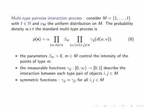
Multi-type pairwise interaction process : consider M = 1, . . . , Iwith I ∈ N and νM the uniform distribution on M. The probabilitydensity w.r.t the standard multi-type process is
p(x) = α∏
(w ,m)∈x
βm∏
(u,i)6=(v ,j)∈x
γij(d(u, v)). (8)
the parameters βm > 0, m ∈ M control the intensity of thepoints of type m.
the measurable functions γij : [0,∞) → [0, 1] describe theinteraction between each type pair of objects i , j ∈ M
symmetric functions : γij ≡ γji for all i , j ∈ M
For (w ,m) /∈ x, the conditional intensity is
λ((w ,m); x) = βm∏
(u,i)∈x
γim(d(u,w)).
This process is locally stable with Λ = maxm∈M βm, anti-monotonicand Markov under smooth assumptions on the functions γij .The interaction functions are
φc(∅) = α
φc((w ,m)) = βm
φc ((u, i), (v , j)) = γij(d(u, v))
with φc ≡ 1 for cliques of three objects and more.
Area interaction model :(Baddeley and van Lieshout, 1995)
p(x) ∝ βn(x)γ−ν[Γ(x)], β, γ > 0 (9)
a) 0 50 100 150 200 250 3000
50
100
150
200
250
300
b) 0 50 100 150 200 250 3000
50
100
150
200
250
300
c) 0 50 100 150 200 250 3000
50
100
150
200
250
300
Figure: Area interaction model realisations for different parametervalues : a) γ = 1.0, b) γ > 1.0 and c) γ < 1.0.
Remarks :
the first probability density based point process producingclusters → alternative to the Strauss process ...
the model should be re-parametrized in order to be identifiable
Proposition
The area interaction process given by (9) is a Markov pointprocess.
Proof.→ blackboard
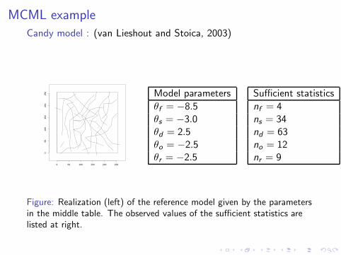
Candy model :
(van Lieshout and Stoica, 2003), (Stoica, Descombes and Zerubia,2004)
p(x) ∝ γnf (x)f γ
ns (x)s γ
nd (x)d γ
no(x)o γ
nr (x)r ,
with γf , γs , γd > 0 and γo , γr ∈ [0, 1]
a)
0 50 100 150 200 250
050
100
150
200
250
b)
0 50 100 150 200 250
050
100
150
200
250
c)
0 50 100 150 200 250
050
100
150
200
250
Figure: Candy model realisations.
Bisous model :(Stoica, Gregori and Mateu, 2005)
p(x) ∝[
q∏
s=0
γns(x)s
]∏
κ∈Γ⊂R
γnκ(x)κ γs > 0, γκ ∈ [0, 1]
020
4060
80100
020
4060
80100
0
10
20
30
40
50
60
70
80
90
100
020
4060
80100
020
4060
80
0
10
20
30
40
50
60
70
80
90
100
020
4060
80100
020
4060
80100
0
10
20
30
40
50
60
70
80
90
100
Figure: Random shapes generated with Bisous model.
Remarks :
Candy and Bisous are based on compound interactions →drawing + explanations
connections are produced by giving different weights for therepulsive interactions
the conditional intensity is bounded
λ(ζ; x) ≤q∏
s=0
maxγs , γ−1s 12 = Λ.
this gives the name of the model → kissing number
→ blackboard - Candy
Markov range : 4rh + 2ra
the models are locally stable but the exact simulation issometimes difficult ...
Compare two random sets : idea inspired by current undergoingwork with M. N. M. van Lieshout and classical literature inmathematical morphology
Figure: Realizations of the Candy model obtained with different samplers.
Empty space function : these probability distributions should besimilar ⇒ Kolmogorov-Smirnov p− value is higher than 0.8
0.00 0.05 0.10 0.15 0.20
0.0
0.2
0.4
0.6
0.8
1.0
Empty space functions for Candy patterns
r
F e
stim
ate
Figure: Estimation of the empty space function for the previous Candyrealizations
J function for multi-type segment pattern : undergoing work withMarie-Colette van Lieshout
undergoing work with Marie-Colette van Lieshout (CWIAmsterdam) and a group of people from CIRAD Montpellier
show : R script testJFuncData.R
Open questions :
may the F function be used to characterize and to comparedifferent filamentary patterns ?
may a general J function be used to characterise theinteractions of filaments, clusters and walls ?
temporal behaviour ? if yes, for what type of model ?
planar and cluster patterns ?
Lesson IIntroductionSome data sets and their related questions
Lesson IIMathematical backgroundDefinition of a point processBinomial point processPoisson point process
Lesson IIIMoment and factorial moment measures, product densitiesMore properties of the Poisson processCampbell moment measuresCampbell - Mecke formula
Lesson IVInterior and exterior conditionningA review of the Palm theorySlivnyak - Mecke theoremApplications : summary statistics
Lesson V
Reduced Palm distributionsCampbell and Slivnyak theoremsSummary statistics : the K and L functionsExterior conditioning : conditional intensity
Lesson VIIProbability density of a point processesInteracting marked point processesMarkov point processes
Lesson VIIIMonte Carlo simulationMarkov chains : a little bit of theoryMetropolis-Hastings algorithmMH algorithm for sampling marked point processesSpatial birth-and-death processes
Perfect or exact simulation
Lesson IXStatistical inference problemsMonte Carlo Maximum likelihood estimationParameter estimation based on pseudo-likelihoodModel validation : residual analysis for point processesStatistical pattern detection
Conclusion and perspectives
Markov chain Monte Carlo algorithms
Problem : sampling or simulation probability distributions
π(A) =
∫
A
p(x)dµ(x)
that are not available in closed form ↔ normalizing constantanalytically intractableRemarks :
almost all the point process models and Markov random fields
exceptions : Poisson processes and also permanental anddeterminental point processes
Markov chain theory and simulation is whole domain inprobability and statistics → very general working framework
Basic MCMC algorithm
Algorithm
x = My first MCMC sampler (T )
1. choose an initial condition x0
2. for i = 1 to T , do
xi = Update(xi−1)
3. return xT .
Principles of the MCMC algorithm :
simulates a Markov chain
the Update function reproduces the transition kernel of theMarkov chain
the output xT is asymptotically distributed according to πwhenever T → ∞
if the simulated Markov chain has good properties →statistical inference is possible
several solutions : Gibbs sampler, Metropolis-Hastings, birthand death processes, stochastic adsorption, RJMCMC, exactsimulation (CFTP, clan of ancestors, etc.)
Markov chains : a little bit of theory
Let (Ω,F , µ) a probability space.
Markov chain : a sequence of random variables Xn such that :
P(Xn+1|X0, . . . ,Xn) = P(Xn+1|Xn)
The chain is homogeneous if the probabilities from going from onestate to another do not change in time.
Transition kernel : it is the “engine” of the Markov chain, that is amapping P : Ω×F → [0, 1] such that
P(·,A) is measurable for any A ∈ F P(x , ·) is a probability measure on (Ω,F) for any fixed x ∈ Ω
Invariant distribution : the probability distribution π that satisfies
π(A) =
∫
Ωπ(dx)P(x ,A), ∀A ∈ F
interpretation : the transition kernel changes of the currentstate, but the new state is distributed according to π
Reversible chain : the probability of going from A to B equals theprobability of going from B to A
∫
B
π(dx)P(x ,A) =
∫
A
π(dx)P(x ,B).
The reversibility implies invariance. Indeed, since P(x ,Ω) = 1 andconsidering B = Ω in the reversibility equations, we get
∫
Ωπ(dx)P(x ,A) =
∫
A
π(dx) = π(A)
Equilibrium distribution : the invariant distribution is anequilibrium distribution if and only if :
limn→∞
Pn(x ,A) = π(A)
for all measurable sets A ∈ F and any x ∈ Ω ; Pn is the n−thapplication of the transition kernel
Markov chains : convergence properties
Important : key elements whenever building a transition kernels
aperiodicity : no deterministic loops
irreducibility : the chain can go from any state to any otherstate
recurrence : the chain can go from any state to any otherstate “often enough” → independence of the initial conditions
ergodicity : the chains distribution converge towards itsequilibrium distribution “fast enough” (an ergodic chain isrecurrent ..)
Proposition
The invariant distribution of an aperiodic and irreducible chain isunique and it is also the equilibrium distribution of the chain.
Remark : the previous result is verified, for all starting pointsx ∈ Ω′ such that π(Ω \ Ω′) = 0. Hence, the convergence dependon the initial conditions. The recurrence property banishes thesenull-sets.
Proposition
The ergodic chain reaches the equilibrium regime, fast enough,from any initial state. The large numbers law and the central limittheorem can be used whenever sampling with an ergodic chain.
Remark : the speed of convergence of the chain may be the samefor all the initial conditions, the chain is uniformly ergodic. If thespeed of convergence depends on the starting a point, we mayhave a geometrically ergodic chain
drift condition : technical mathematical tool for establishingconvergence properties of a Markov chain
Metropolis-Hastings algorithm
Principle :
consider the chain in the state xi = x
propose a new state xf = y using the proposal densityq(xi → xf )
accept this new state with probability
α(x , y) = min
1,
p(y)q(y → x)
p(x)q(x → y)
if not remain in the previous state
iterate as many times as we need (... in theory till infinity ...)
Properties
α(·, ·) is a solution of the detailed balance equation →reversibility is preserved
very few conditions are required for q(· → ·) so that the chainhas all the convergence properties
q(· → ·) should be simple to calculate and to simulate
the knowledge of the normalizing constant of p(·) is notneeded
→ blackboard + Exercise 12 + comment Elmo
MH algorithm for sampling marked point processes
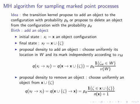
Idea : the transition kernel propose to add an object to theconfiguration with probability pb or propose to delete an objectfrom the configuration with the probability pdBirth : add an object
initial state : xi = x an object configuration
final state : xf = x ∪ ζ proposal density to add an object : choose uniformly its
location in W and its mark independently according to νM
q(xi → xf ) = q(x → x ∪ ζ) = pb1ζw ∈ W ν(W )
proposal density to remove an object : choose uniformly anobject from x ∪ ζ
q(xf → xi) = q(x ∪ ζ → x) = pd1ζ ∈ x ∪ ζ
n(x) + 1
acceptance probability
α(x → x ∪ ζ) = min
1,
pdp(x ∪ ζ)pbp(x)
× ν(W )
n(x) + 1
(10)
Death : remove an object
the inverse movement of birth
acceptance probability
α(x → x \ ζ) = min
1,
pbp(x \ ζ)pdp(x)
× n(x)
ν(K )
(11)
Remark : note the appearance of the Papangelou intensity in theacceptance probability ⇒ local stability property guarantees goodconvergence properties of the Markov chain
A transition kernel doing these transformations is
P(x,A) = pb
∫
K
b(x, η)α(x, y := x ∪ η)1y ∈ Adσ(η)
+ pd∑
η∈x
d(x, η)α(x, y := x \ η)1y ∈ A
+ 1x ∈ A[1− pb
∫
K
b(x, η)α(x, x ∪ η)dσ(η)
− pd∑
η∈x
d(x, η)α(x, x \ η)],
where K = W ×M, dσ(η) = dσ((w ,m)) = dν(w)× dνM(m) et0 < pb + pd ≤ 1. The birth rate is b(x, η) = 1
ν(W ) and the death
rate is d(x, η) = 1n(x)
Algorithm
y = Update(x)
1. Choose “birth” or “death” with probabilities pb and pd ,respectively.
2. If “birth” was chosen, then generate a new object followingb(x, η). Accept the new configuration, y = x ∪ η with theprobability α(x, y) given by (10).
3. If “death” was chosen, then select the object to be removedusing d(x, η). Accept the new configuration, y = x \ η withthe probability α(x, y) given by (11).
4. Return the present configuration.
TheoremLet be b, d and q as described previously. Assume that b(x, η) andd(x, η) are strictly positive on their corresponding definitiondomain, respectively, and
limn→∞
un = limn→∞
[sup
η∈W×M,x∈Ξn
d(x ∪ η, η)b(x, η)
]→ 0.
Fix pb, pd ∈ (0, 1) with pb + pd ≤ 1 and let p(x) be the probabilitydensity of a marked point process on W ×M. The point process islocally stable and p(x) is built w.r.t the standard Poisson processµ. The MH sampler defined previously simulates a Markov chainwith invariant measure π =
∫pdµ who is φ−irreducible, Harris
recurrent and geometric ergodic.
Remark :
the same result holds if change moves are introduced withcare ... → explain ...
Optimality of the MH dynamics
theoretical convergence properties
local computation
no need of the normalising constant
highly correlated samples : only one element changed peraccepted transition
allows improvements : transition kernels that “help” themodel
Tailored to the model proposal distribution
b(x, η) =p1ν(K )
+ p2ba(x, η),
with p1 + p2 = 1 and ba(x, η) a probability density given by
ba(x, η) =1
n(A(x))
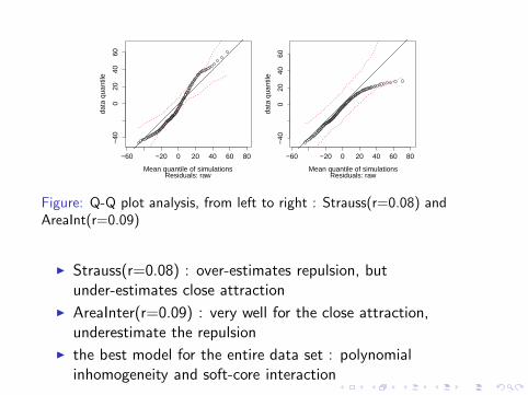
∑
x∈A(x)
b(x , η).
the role of ba(x, η) : propose the birth of a new pointin thoseregions where the interactions between the new born and theother configuration members is favoured or not penalised bythe model
A(x) : the set of marked points in a configuration that are notexhibiting yet “good” interactions
Figure: Extremities marked by triangles are connected and further than12 lmax + rc to the boundary, those labeled by a black disk are closer than12 lmax + rc to the boundary of K .
MH algorithm for sampling the Candy model : dynamics behaviourthrough the sufficient statistics analysis
0.2 0.4 0.6 0.8 1 1.2 1.4 1.6 1.8 2
x 104
0
0.5
1
1.5
2
2.5
3
3.5
4
4.5
5
0.2 0.4 0.6 0.8 1 1.2 1.4 1.6 1.8 2
x 104
24
25
26
27
28
29
30
31
32
nf = 3.64 ns = 28.63
0.2 0.4 0.6 0.8 1 1.2 1.4 1.6 1.8 2
x 104
55
60
65
70
75
0.2 0.4 0.6 0.8 1 1.2 1.4 1.6 1.8 2
x 104
7
7.5
8
8.5
9
9.5
10
10.5
11
nd = 64.07 no = 8.82
great adaptability and theoretical convergence
easy to use
but appropriate solutions need to be found for each newproblem or situation ...
the dynamics has to be built depending on the model
the general framework, even if having good theoreticalproperties, it is not always the most efficient from a numericalpoint of view ...
but if you do not have good theoretical properties, yourresults will be bad anyway ...
Spatial birth-and-death processes
Theoretical background : continuous time Markov chains → thevery nice book of S. Resnick (2005)
history : the first MCMC sampler for marked point processes
the simulation of locally stable marked point process is verysimple
thinning procedure
the simulated pattern is “hidden” in a dominating Poissonprocess
Algorithm
Let p be the probability density w.r.t. the standard Poissonprocess, of a locally stable marked point process on W ×M. Itscorresponding Papangelou conditional intensity bound is Λ.
1. Simulate a Poisson process on W ×M with intensity functionρ = Λ. Let xΛ be the obtained configuration.
2. Set x = ∅ the realisation of p, and continue
3. For every point η in xΛ do
the point is added to x : x = x ∪ η with probability
λ(η; xΛ)
Λ
otherwise the point is deleted from xΛ : xΛ = xΛ \ η4. Return x
Remarks :
this algorithm has all the desired convergence properties
comparing with MH algorithm, this algorithm may easilyproduce independent samples ...
nevertheless, for strong interactions Λ may be very high
Candy and Bisous models with strong interactions cannot besimulated with this algorithm
Perfect or exact simulation
classical MCMC methods → need a theoretical infinite timetill convergence
dependence on the initial conditions
perfect or exact MCMC methods indicate by themselveswhenever the convergence is attained
these methods are perfect within the limits of the randomnumber generators of the computers
historical paper : (Propp and Willson, 1996)
Principle : discrete case
Let us build a MCMC sampler for π defined on the discrete statespace Ω = ω1, ω2, . . . , ωm. The induced Markov chain (Xn) isrepresented by its transition functiones φ(·, ·) such that
Xn+1 = φ(Xn,Vn), (12)
where Vn are i.i.d random variables.
Key idea :
consider m, (Xn(ωi )) all initialised with a different state, thatevolve from −T < 0 till 0
the chains are coupled : they use the same Vns
if at a certain moment n ∈ −T , . . . , 0 all the chains are in thesame state or they coalesced, that is
Xn ≡ x
then they will all remain in the same state, till the time 0
the influence of the initial conditions just ... vanished
if the chains are started before the time −T , at infinite, thechains will be all in the same state, at the same moment
it comes out that X0 is a perfect sampler from the equilibriumdistribution π
→ blackboard drawing
Extraordinary smart idea :
launching m parallel chains is not always feasible
if Ω can be ordered
ωmin = ω(1) < ω(2) < . . . < ω(m) = ωmax
and if the transition kernel respect this order relation
ω ≤ ω′ ⇒ φ(ω) ≤ φ(ω′)
then only the states ωmin and ωmax are needed
the behaviour of the other chains is bounded by the extremalchains Xn(ωmin) and Xn(ωmax)
This idea is known under the name Coupling From The Past(CFTP).
Perfect algorithms for sampling marked point processes
Previous ideas hold for perfect sampling of marked point processesCFTP based algorithms :
spatial birth-and-death and clan of ancestors : thinningprinciples
Metropolis-Hastings
locally stable point processes
monotonic and anti-monotonic point processes
dominating process : stationary Poisson → (CFTP and clan ofancestors), Λ parameter is important
the transition function ingredients : conditional intensity, Λand the Vns
Gibbs sampler algorithm :
discrete probability densities → approximation of thecontinuous marked point processes probability density
does not require : order relation, dominating process,monotonic or anti-monotonic relation
still the algorithm is more efficient if these properties areexhibited by the considered model
Potts like models
Remarks :
CFTP algorithm is implemented within the spatstat package
all these algorithms are implemented within the MPPLIB
C++ package
Strauss model : convergence speed for exact sampling methods
(van Lieshout and Stoica, 2006)
a) 0
0.05
0.1
0.15
0.2
0
50
100
1500
2000
4000
6000
8000
10000
12000
14000
b) 0
0.02
0.04
0.06
0.08
0
20
40
60
80
1000
500
1000
1500
2000
2500
3000
3500
c) 0
0.05
0.1
0.15
0.2
0
50
100
1500
2
4
6
8
10
12
x 104
d) 00.02
0.040.06
0.080.1
0.120.14
0
20
40
60
80
1003000
4000
5000
6000
7000
8000
9000
10000
Figure: Exact simulation algorithms applied to Strauss model : a) CFTP,b) clan of ancestors, c) Metropolis-Hastings and d) Gibbs.
Comparison exact simulation and MH algorithm for the
Strauss model (1)
2040
6080
Comparison Strauss statistics distributions
2040
6080
2040
6080
Figure: Boxplots comparison for the n and sr statistics distributions :white - the distributions obtained using the exact algorithm, pink (darkcouloured) - the distributions obtained using the Metropolis - Hastingsalgorithm.
Comparison exact simulation and MH algorithm for the
Strauss model (2)
60 70 80 90
5060
7080
90
Total number of points distribution
Exact quantiles
MH
qua
ntile
s
5 10 15 20
510
1520
Interacting pairs distribution
Exact quantiles
MH
qua
ntile
s
Figure: Qqplot comparison for the n and sr statistics distributions.
Open questions MCMC methods :
Classical algorithms - MH based dynamics
good convergence properties but convergence at infinity
burning-in methods + de-correlation techniques
great adaptability : tailored to the model moves
manipulate several objects during one move : work of X.Descombes
link with RJMCMC : great adaptability, but difficult to stateconvergence proofs, hence difficult to use ...
Perfect simulation algorithms
the simulated chain indicates by itself whenever convergenceis reached
parameter dependence : can be applied in practice only to arestricted range of parameters
neither change moves, nor tailored moves
study existing algorithm : Fill algorithm, forward simulationand simulated tempering
challenging perspective : synthesis of both families ofalgorithms → exact algorithms able to be tailored to themodel
Lesson IIntroductionSome data sets and their related questions
Lesson IIMathematical backgroundDefinition of a point processBinomial point processPoisson point process
Lesson IIIMoment and factorial moment measures, product densitiesMore properties of the Poisson processCampbell moment measuresCampbell - Mecke formula
Lesson IVInterior and exterior conditionningA review of the Palm theorySlivnyak - Mecke theoremApplications : summary statistics
Lesson V
Reduced Palm distributionsCampbell and Slivnyak theoremsSummary statistics : the K and L functionsExterior conditioning : conditional intensity
Lesson VIIProbability density of a point processesInteracting marked point processesMarkov point processes
Lesson VIIIMonte Carlo simulationMarkov chains : a little bit of theoryMetropolis-Hastings algorithmMH algorithm for sampling marked point processesSpatial birth-and-death processes
Perfect or exact simulation
Lesson IXStatistical inference problemsMonte Carlo Maximum likelihood estimationParameter estimation based on pseudo-likelihoodModel validation : residual analysis for point processesStatistical pattern detection
Conclusion and perspectives
Statistical inference problems
Problem I : parameter estimation
observe the pattern x and find the model parameters θ able tostatistically reproduce it
complete and incomplete data : Monte Carlo maximumlikelihood, pseudo-likelihood, EM ...
open problem : sampling p(θ|x) ...Problem II : pattern detection
observe the data d and find x “hidden”
the model parameters are : hidden, modelled, unknown
open problem : the detected pattern does it really exist ...?
Problem III : sample the joint law of the pattern and theparameters p(x, θ)
shape modelling → “crystal ball” ?
observe a phenomenon and propose a model doing the“same” ...
needs the time dimension
open problem : time,
what it is the time “quanta” → generating element andinteractions as for marked point processes ?
Monte Carlo Maximum likelihood estimation
Exponential family models :
very general framework
the point processes models that were presented are given by
p(x|θ) = exp〈t(x), θ〉Z (θ)
where t(x) and θ represent the sufficient statistics vector andthe model parameters vector, respectively. The normalisingconstant Z (θ) is unknown.
The configuration x is entirely observed, hence the log-likelihoodwith respect a known parameter ψ can be written as follows :
l(θ) = 〈t(x), θ − ψ〉 − logZ (θ)
Z (ψ)
It is easy to check, that the normalizing constants ratio is
Z (θ)
Z (ψ)= E [exp〈t(X), θ − ψ〉] ,
since we have
Z (θ)
Z (ψ)=
1
Z (ψ)
∫
Ωp(x|θ)dµ(x)
=1
Z (ψ)
∫
Ωp(x|θ)p(x|ψ)
p(x|ψ)dµ(x)
=
∫
Ω
p(x|θ)p(x|ψ)
p(x|ψ)Z (ψ)
dµ(x)
= E
[p(X|θ)p(X|ψ)
]
The Monte Carlo approximation of the normalizing constants ratiogives :
Z (θ)
Z (ψ)≈ 1
n
n∑
i=1
exp〈t(Xi), θ − ψ〉,
where X1,X2, . . . ,Xn are samples obtained from p(y|ψ).Hence, the Monte-Carlo counterpart of the log-likelihood is :
ln(θ) = 〈t(x), θ − ψ〉 − log
(1
n
n∑
i=1
exp〈t(Xi), θ − ψ〉).
TheoremThe log-likelihood of an exponential family model is a convexfunction.
proof : see (Monfort 1997, Thm.3, pp. 61)
ln(θ) → l(θ) almost sureley
all these suggest that local optimisation procedures applied toln(θ) may give interesting results
MCMC local optimisation procedures
The gradient of the MCMC log-likelihood is
∇ln(θ) = t(x)− En,θ,ψ[t(X)]
where
En,θ,ψ[t(X)] =
∑ni=1 t(Xi) exp〈t(Xi), θ − ψ〉∑n
i=1 exp〈t(Xi ), θ − ψ〉that is the Monte Carlo importance sampling approximationof Eθt(X).
where ρ(θk) is the optimal step (Descombes et al. ’99, Stoica ’01).
re-sampling if ‖ θk − ψ ‖> threshold
obtain a reference value θ0 close enough to the maximumlikelihood estimator
Asymptotic results
The random variable√n(θn − θ) whenever n → ∞, it converges in
distribution towards a normal random variable of zero mean andvariance I (θ)−1ΓI (θ)−1 :
√n(θn − θ) → N (0, I (θ)−1ΓI (θ)−1).
the matrixI (θ) = Var
θ[t(X)] = −∇2l(θ)
is the Fisher information of θ
the matrix Γ is the matrix of asymptotic covariance of thenormalised Monte Carlo gradient
√n∇ln(θ)
an approximation of these matrices may be found in (vanLieshout and Stoica, 2003)
under some assumptions, the error θ − θ0 can be estimated bythe diagonal of the inverse of −∇2ln(θn)
MCML example
Candy model : (van Lieshout and Stoica, 2003)
0 50 100 150 200 250
050
100
150
200
250 Model parameters
θf = −8.5θs = −3.0θd = 2.5θo = −2.5θr = −2.5
Sufficient statistics
nf = 4ns = 34nd = 63no = 12nr = 9
Figure: Realization (left) of the reference model given by the parametersin the middle table. The observed values of the sufficient statistics arelisted at right.
Results : estimation of the parameters from the referenceconfiguration given by the Candy model
Figure: Monte Carlo approximation of the log likelihood function. The Xaxis represents the variation of a single component. The Y axisrepresents the values of the Monte Carlo log likelihood with all othercomponents of θ0 fixed : a - θf ∈ [−11,−7], b - θs ∈ [−5,−1], c -θd ∈ [1, 5], d - θo ∈ [−4.5,−0.5], e - θr ∈ [−4.5,−0.5].
Parameter estimation based on pseudo-likelihood
The pseudo-likelihood of a marked point process X with conditionalintensity λθ(ζ; x) observed on the bounded set W is expressed as
PLW (θ; x) =
=
[∏
xi∈x
λθ(xi ; x)
]exp
[−∫
W×M
λθ((w ,m); x)ν(dw)νM (dm)
].
The pseudo-likelihood estimator is given by the solution of theequation :
∂PLW (θ; x)
∂θ= 0
Properties :
the PL is concave for exponential models
no normalising constant needed ...
it ”amplifies” the interaction weights : check the formula - fora Strauss process the interactions are counted twice ...
consistency and asymptotic normality of the estimator : if weobserve the model in a finite window, then it convergestowards the parameters estimated based on the “whole”window (Jensen and Møller, 1991)
lacks of statistical significance (except for the Poissonprocess) : there is no real link with the true model behind thepattern
but easy to be implemented : this was the motivation tointroduce it in the middle of 70s (Besag, 1975)
Implementation within R spatstat package
stationary Strauss process :
log λθ(ζ; x) = log β + (log γ)t(ζ, x)
with t(ζ, x) the number of pairs of objects closer than thedistance r in the configuration y
general structure of the conditional intensity
log λθ(ζ; x) = ηS(ζ) + φV (ζ, x),
with the ‘first order term’ S(u) that describes spatialinhomogeneity and/or covariates effects and the ‘higher order’term that describes interobject interaction
refer to the spatstat documentation
Applications
Pseudo-likelihood profile analysis : the range parameters>radius = data.frame(r=seq(0.05,0.11, by=0.01))
Pearson residuals h(η, x) = 1/√λ(η; x) (analogy with Poisson
log-linear regression)
R(A,1√λ, θ) =
∑
xi∈xA
1√λ(xi ; xA)
−∫
A
√λ(η; x)(ν × νM)(dη)
RemarkThe inverse and Pearson residuals we need λθ(x)(xi ; x) > 0 for allxi ∈ x for any pattern yy , while λθ(x)(η; x) = 0 is allowed for η /∈ x
Properties
expectation
E
[R(A, h, θ)
]
=
∫
A
E
[hθ(X∪η)
(η,X)λ(η,X) − hθ(X)
(η,X)λθ(X)
(η,X)]
variance : more complicate structures but very nice formulasfor Poisson processes (Baddeley, Moller and Pakes 2008)
these residuals do not have independent increments → theraw innovations for Markov point processes are conditionnalyindependent and uncorrelated (Baddeley, 2005)
consistency and asymptotic normality for the residuals ofstationary Gibbs point processes (Coeurjolly and Lavancier,2013)
Application : smoothed residuals to test several models forjapanesepines datasets
Strauss process : only repulsion
area-interaction process : repulsion or attraction (competitionfor ressources)
−70
−60
−50
−40
−56
.8−
56.4
−56
Figure: Raw residual analysis, from left to right : Strauss(r=0.08) andAreaInt(r=0.09)
R code>mjp=ppm(japanesepines, 1,Strauss(r=0.08),rbord=0.08)
>rjp=residuals(mjp,type="raw")
>plot(rjp)
QQ plots : comparison of empirical quantiles of the smoothedresiduals with the expected quantiles under the estimated model
interpretation in the spirit of K and F functions
if the data pattern is more clustered than the model : heaviertails especially in the left-hand tail
if the data pattern is more inhibited than the model : lightertails especially in the right-hand tail
R code : qqplot.ppm(rjp, type="raw")
−60 −20 0 20 40 60 80
−40
020
4060
Mean quantile of simulations
data
qua
ntile
Residuals: raw
−60 −20 0 20 40 60 80
−40
020
4060
Mean quantile of simulations
data
qua
ntile
Residuals: raw
Figure: Q-Q plot analysis, from left to right : Strauss(r=0.08) andAreaInt(r=0.09)
Strauss(r=0.08) : over-estimates repulsion, butunder-estimates close attraction
AreaInter(r=0.09) : very well for the close attraction,underestimate the repulsion
the best model for the entire data set : polynomialinhomogeneity and soft-core interaction
Remarks :
the theory is wonderful
but the numerical results are obtained using the PL estimators...
see the remark of J. Besag
visualisation of residuals difficult for higher dimensions
the qq plots very informative → link with the central limittheorems for computing confidence intervals
open question : validating pattern detection result ... ?
Statistical pattern detectionBuild the pattern model : probability density constructionconditionally on the data observation
p(x, θ|d) ∝ exp
[−Ud(x|θ) + Ui (x|θ)
Z (θ)+ log p(θ)
]
interaction energy Ui(x|θ) → objects interactions (geometricalshape of the structure)
data energy Ud(x|θ) induced by the data field d → objectlocations
if the interaction parameters are unknown → prior model p(θ)
Pattern estimator : the object configuration that maximises theprobability density
(x, θ) = arg minΩ×Ψ
Ud(x|θ) + Ui(x|θ)
Z (θ)− log p(θ)
with Ψ the model parameters space
Simulated annealing : global optimisation technique
sampling from p(x, θ)1/T while slowly T → 0
convergence towards the uniform distribution on theconfiguration subspace minimizing U(x, θ) (Stoica, Gregoriand Mateu, 2005)
inhomogeneous Markov chain ...
Algorithm
x = Simulated Annealing (T0, δ,T )
1. choose an initial condition x0
2. for i = 1 to T do
xi = Update (xi−1,Ti−1, δ)Ti = T0/[log(i) + 1]
3. return xT .
Level sets estimators :
visit maps for compact regions in K (Heinrich, Stoica andTran, 2012) :
T (x) > α ⇒ Tn(x) > α
two challenges : discretisation and Monte Carloapproximations
average behaviour of the pattern (fixed temperature)
Build the machine ...Galaxies catalogs :
interaction energy : Bisous model (random cylinders) data energy : local tests (density and spread of galaxies inside
a cylinder)
ily
iy
y
i+ky
i+k
i+k
l
w
ir
Figure: Locating interacting cylinders in a field of points.
Epidemiological data :
interaction energy : Strauss and Area-interaction model(random disks)
data energy : local statistical test (the average score of thefarms covered by a disk)
a) b)
Figure: Data→ field of marked points : a) observed clusters, b) clustersapproximated by random disks.
Road network extraction
(Stoica, Descombes, van Lieshout and Zerubia, 2002)
a) b)
Figure: Rural region in Malaysia : a) original image; b) obtained results.
Forest galleries : verifying the results(Stoica, Descombes and Zerubia, 2004)
a) b)
c) d)
Figure: Forest galleries extraction : a) original image ; b) ground truth ;c)-d) obtained results. Data provided by BRGM.
Figure: Detected filamentary pattern (cylinder axes) in a small samplevolume within a pattern of galaxies (points).
Galaxy catalogue (2)
(Tempel, Stoica et. al., 2014)The movie, showing the MCMC in action is available at:http://www.aai.ee/ elmo/sdss-filaments/
Epidemiology : sub-clinical mastitis data
(Stoica, Gay and Kretzschmar, 2007)
a) 0 50 100 150 200 250 300 350
50
100
150
200
250
300
b) 0 50 100 150 200 250 300
50
100
150
200
250
300
0
0.1
0.2
0.3
0.4
0.5
0.6
0.7
0.8
0.9
1
Figure: Disease data scores and coordinates for the year 1996 : a) diskconfiguration obtained using the simulated annealing algorithm ; b) coverprobabilities.
Does the detected pattern really exist ?
Idea : the sufficient statistics of the model → morphologicaldescriptors of the shape hidden by the data
turn the machine at constant temperature T = 1
compute the average of the sufficient statistics
compare with the maximum value obtained for the permuteddata
Sufficient statistics :
Bisous model (pattern of connected cylinders) : free cylinders,cylinders with one extremity connected, cylinders with bothextremities connected
Test for the galaxy catalogs
Permuted data : keeping the same number of galaxies whilespreading them uniformly (binomial point process)
Permuted data : keeping the same farm locations while exchangingthe score disease
Results :
sufficient statistics for the data from the year 1996 :
n(y) = 74.10, ν[Z (y)] = 312.46, no = 555.08
maximum values of the sufficient statistics for 100 simulateddata fields
n(y) = 2.36, ν[Z (y)] = 13.83, no = 2.62
Interpretation : this test does not say if the pattern is welldetected, but it says that there is something to be detected ...
How similar are two data sets ?
Cosmology : compare the sufficient statistics for 22 mockcatalogues with the ones for the observation (Stoica, Martinez andSaar, 2010)
Discussion
mock catalogues exhibit filaments
mock filaments are generally shorter, more fragmented andmore dense
Bisous model : good for testing the filamentary structure
1 2 3 4 5 6 7 8 9 11 13 15 17 19 21 23
05
1015
200
510
1520
Distribution of the n0 statistics
1 2 3 4 5 6 7 8 9 11 13 15 17 19 21 23
010
2030
400
1020
3040
Distribution of the n1 statistics
1 2 3 4 5 6 7 8 9 11 13 15 17 19 21 23
02
46
80
24
68
Distribution of the n2 statistics
Figure: Comparison of the sufficient statistics distributions for the realdata (dark box plot) and the mock catalogues.
Spatial models and random geometry :
Markov marked point processes allow statistical andmorphological description of the pattern
good synthesis properties
limitations : models remain just models ...
Perspectives :
random geometry (marked point processes, random fields) →modelling, simulation, statistical inference
temporal dimension ...
applications : astronomy and environmental sciences
Acknowledgements :
this work was done together with wonderful co-authors and alsowith the precious help of some very generous persons ... Some ofthem are today with us :) ...