152
Mathematical Statistics Sara van de Geer September 2015
Mathematical Statistics
Sara van de Geer
September 2015

2
Contents
1 Introduction 71.1 Some notation and model assumptions . . . . . . . . . . . . . . . 71.2 Estimation . . . . . . . . . . . . . . . . . . . . . . . . . . . . . . 101.3 Comparison of estimators: risk functions . . . . . . . . . . . . . . 121.4 Comparison of estimators: sensitivity . . . . . . . . . . . . . . . . 121.5 Confidence intervals . . . . . . . . . . . . . . . . . . . . . . . . . 13
1.5.1 Equivalence confidence sets and tests . . . . . . . . . . . . 131.6 Intermezzo: quantile functions . . . . . . . . . . . . . . . . . . . 141.7 How to construct tests and confidence sets . . . . . . . . . . . . . 141.8 An illustration: the two-sample problem . . . . . . . . . . . . . . 16
1.8.1 Assuming normality . . . . . . . . . . . . . . . . . . . . . 171.8.2 A nonparametric test . . . . . . . . . . . . . . . . . . . . 181.8.3 Comparison of Student’s test and Wilcoxon’s test . . . . . 20
1.9 How to construct estimators . . . . . . . . . . . . . . . . . . . . . 211.9.1 Plug-in estimators . . . . . . . . . . . . . . . . . . . . . . 211.9.2 The method of moments . . . . . . . . . . . . . . . . . . . 221.9.3 Likelihood methods . . . . . . . . . . . . . . . . . . . . . 23
2 Decision theory 292.1 Decisions and their risk . . . . . . . . . . . . . . . . . . . . . . . 292.2 Admissibility . . . . . . . . . . . . . . . . . . . . . . . . . . . . . 312.3 Minimaxity . . . . . . . . . . . . . . . . . . . . . . . . . . . . . . 332.4 Bayes decisions . . . . . . . . . . . . . . . . . . . . . . . . . . . . 342.5 Intermezzo: conditional distributions . . . . . . . . . . . . . . . . 352.6 Bayes methods . . . . . . . . . . . . . . . . . . . . . . . . . . . . 362.7 Discussion of Bayesian approach . . . . . . . . . . . . . . . . . . 392.8 Integrating parameters out . . . . . . . . . . . . . . . . . . . . . 412.9 Intermezzo: some distribution theory . . . . . . . . . . . . . . . . 42
2.9.1 The multinomial distribution . . . . . . . . . . . . . . . . 422.9.2 The Poisson distribution . . . . . . . . . . . . . . . . . . . 432.9.3 The distribution of the maximum of two random variables 44
2.10 Sufficiency . . . . . . . . . . . . . . . . . . . . . . . . . . . . . . . 452.10.1 Rao-Blackwell . . . . . . . . . . . . . . . . . . . . . . . . . 472.10.2 Factorization Theorem of Neyman . . . . . . . . . . . . . 482.10.3 Exponential families . . . . . . . . . . . . . . . . . . . . . 502.10.4 Canonical form of an exponential family . . . . . . . . . . 51
3
4 CONTENTS
2.10.5 Minimal sufficiency . . . . . . . . . . . . . . . . . . . . . . 56
3 Unbiased estimators 593.1 What is an unbiased estimator? . . . . . . . . . . . . . . . . . . . 593.2 UMVU estimators . . . . . . . . . . . . . . . . . . . . . . . . . . 60
3.2.1 Complete statistics . . . . . . . . . . . . . . . . . . . . . . 633.3 The Cramer-Rao lower bound . . . . . . . . . . . . . . . . . . . . 663.4 Higher-dimensional extensions . . . . . . . . . . . . . . . . . . . . 703.5 Uniformly most powerful tests . . . . . . . . . . . . . . . . . . . . 72
3.5.1 An example . . . . . . . . . . . . . . . . . . . . . . . . . . 723.5.2 UMP tests and exponential families . . . . . . . . . . . . 753.5.3 Unbiased tests . . . . . . . . . . . . . . . . . . . . . . . . 783.5.4 Conditional tests . . . . . . . . . . . . . . . . . . . . . . . 80
4 Equivariant statistics 854.1 Equivariance in the location model . . . . . . . . . . . . . . . . . 854.2 Equivariance in the location-scale model . . . . . . . . . . . . . . 91
5 Proving admissibility and minimaxity 955.1 Minimaxity . . . . . . . . . . . . . . . . . . . . . . . . . . . . . . 965.2 Admissibility . . . . . . . . . . . . . . . . . . . . . . . . . . . . . 985.3 Inadmissibility in higher-dimensional settings . . . . . . . . . . . 104
6 Asymptotic theory 1076.1 Types of convergence . . . . . . . . . . . . . . . . . . . . . . . . . 107
6.1.1 Stochastic order symbols . . . . . . . . . . . . . . . . . . . 1096.1.2 Some implications of convergence . . . . . . . . . . . . . . 109
6.2 Consistency and asymptotic normality . . . . . . . . . . . . . . . 1116.2.1 Asymptotic linearity . . . . . . . . . . . . . . . . . . . . . 1116.2.2 The δ-technique . . . . . . . . . . . . . . . . . . . . . . . 112
6.3 M-estimators . . . . . . . . . . . . . . . . . . . . . . . . . . . . . 1146.3.1 Consistency of M-estimators . . . . . . . . . . . . . . . . . 1166.3.2 Asymptotic normality of M-estimators . . . . . . . . . . . 119
6.4 Plug-in estimators . . . . . . . . . . . . . . . . . . . . . . . . . . 1256.4.1 Consistency of plug-in estimators . . . . . . . . . . . . . . 1276.4.2 Asymptotic normality of plug-in estimators . . . . . . . . 128
6.5 Asymptotic relative efficiency . . . . . . . . . . . . . . . . . . . . 1316.6 Asymptotic Cramer Rao lower bound . . . . . . . . . . . . . . . 133
6.6.1 Le Cam’s 3rd Lemma . . . . . . . . . . . . . . . . . . . . . 1366.7 Asymptotic confidence intervals and tests . . . . . . . . . . . . . 139
6.7.1 Maximum likelihood . . . . . . . . . . . . . . . . . . . . . 1416.7.2 Likelihood ratio tests . . . . . . . . . . . . . . . . . . . . . 145
6.8 Complexity regularization (to be written) . . . . . . . . . . . . . 149
7 Literature 151

CONTENTS 5
These notes in English closely follow Mathematische Statistik, by H.R. Kunsch(2005). Mathematische Statistik can be used as supplementary reading materialin German.
Mathematical rigor and clarity often bite each other. At some places, not allsubtleties are fully presented. A snake will indicate this.

6 CONTENTS
Chapter 1
Introduction
Statistics is about the mathematical modeling of observable phenomena, usingstochastic models, and about analyzing data: estimating parameters of themodel and testing hypotheses. In these notes, we study various estimation andtesting procedures. We consider their theoretical properties and we investigatevarious notions of optimality.
1.1 Some notation and model assumptions
The data consist of measurements (observations) x1, . . . , xn, which are regardedas realizations of random variables X1, . . . , Xn. In most of the notes, the Xi
are real-valued: Xi ∈ R (for i = 1, . . . , n), although we will also consider someextensions to vector-valued observations.
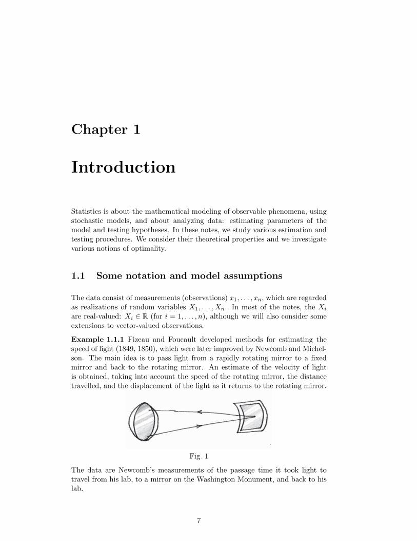
Example 1.1.1 Fizeau and Foucault developed methods for estimating thespeed of light (1849, 1850), which were later improved by Newcomb and Michel-son. The main idea is to pass light from a rapidly rotating mirror to a fixedmirror and back to the rotating mirror. An estimate of the velocity of lightis obtained, taking into account the speed of the rotating mirror, the distancetravelled, and the displacement of the light as it returns to the rotating mirror.
Fig. 1
The data are Newcomb’s measurements of the passage time it took light totravel from his lab, to a mirror on the Washington Monument, and back to hislab.
7
8 CHAPTER 1. INTRODUCTION
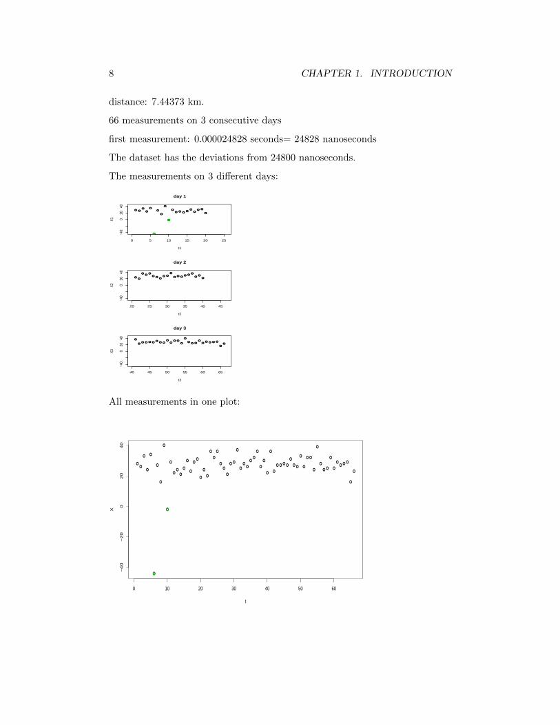
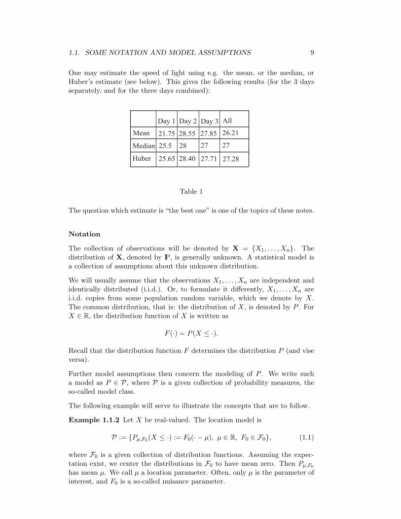
distance: 7.44373 km.
66 measurements on 3 consecutive days
first measurement: 0.000024828 seconds= 24828 nanoseconds
The dataset has the deviations from 24800 nanoseconds.
The measurements on 3 different days:
0 5 10 15 20 25
−40
020
40
day 1
t1
X1
20 25 30 35 40 45
−40
020
40
day 2
t2
X2
40 45 50 55 60 65
−40
020
40
day 3
t3
X3
All measurements in one plot:
0 10 20 30 40 50 60
−4
0−
20
02
04
0
t
X
1.1. SOME NOTATION AND MODEL ASSUMPTIONS 9
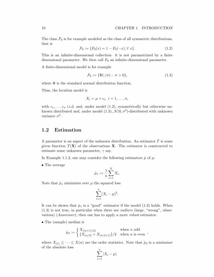
One may estimate the speed of light using e.g. the mean, or the median, orHuber’s estimate (see below). This gives the following results (for the 3 daysseparately, and for the three days combined):
Mean
Median
Huber
Day 1 Day 2 Day 3 All
21.75 28.55 27.85 26.21
25.5 28 27 27
25.65 28.40 27.71 27.28
Table 1
The question which estimate is “the best one” is one of the topics of these notes.
Notation
The collection of observations will be denoted by X = X1, . . . , Xn. Thedistribution of X, denoted by IP, is generally unknown. A statistical model isa collection of assumptions about this unknown distribution.
We will usually assume that the observations X1, . . . , Xn are independent andidentically distributed (i.i.d.). Or, to formulate it differently, X1, . . . , Xn arei.i.d. copies from some population random variable, which we denote by X.The common distribution, that is: the distribution of X, is denoted by P . ForX ∈ R, the distribution function of X is written as
F (·) = P (X ≤ ·).
Recall that the distribution function F determines the distribution P (and viseversa).
Further model assumptions then concern the modeling of P . We write sucha model as P ∈ P, where P is a given collection of probability measures, theso-called model class.
The following example will serve to illustrate the concepts that are to follow.
Example 1.1.2 Let X be real-valued. The location model is
P := Pµ,F0(X ≤ ·) := F0(· − µ), µ ∈ R, F0 ∈ F0, (1.1)
where F0 is a given collection of distribution functions. Assuming the expec-tation exist, we center the distributions in F0 to have mean zero. Then Pµ,F0
has mean µ. We call µ a location parameter. Often, only µ is the parameter ofinterest, and F0 is a so-called nuisance parameter.
10 CHAPTER 1. INTRODUCTION
The class F0 is for example modeled as the class of all symmetric distributions,that is
F0 := F0(x) = 1− F0(−x),∀ x. (1.2)
This is an infinite-dimensional collection: it is not parametrized by a finitedimensional parameter. We then call F0 an infinite-dimensional parameter.
A finite-dimensional model is for example
F0 := Φ(·/σ) : σ > 0, (1.3)
where Φ is the standard normal distribution function.
Thus, the location model is
Xi = µ+ εi, i = 1, . . . , n,
with ε1, . . . , εn i.i.d. and, under model (1.2), symmetrically but otherwise un-known distributed and, under model (1.3), N (0, σ2)-distributed with unknownvariance σ2.
1.2 Estimation
A parameter is an aspect of the unknown distribution. An estimator T is somegiven function T (X) of the observations X. The estimator is constructed toestimate some unknown parameter, γ say.
In Example 1.1.2, one may consider the following estimators µ of µ:
• The average
µ1 :=1
n
N∑i=1
Xi.
Note that µ1 minimizes over µ the squared loss
n∑i=1
(Xi − µ)2.
It can be shown that µ1 is a “good” estimator if the model (1.3) holds. When(1.3) is not true, in particular when there are outliers (large, “wrong”, obser-vations) (Ausreisser), then one has to apply a more robust estimator.
• The (sample) median is
µ2 :=
X((n+1)/2) when n oddX(n/2) +X(n/2+1)/2 when n is even
,
where X(1) ≤ · · · ≤ X(n) are the order statistics. Note that µ2 is a minimizerof the absolute loss
n∑i=1
|Xi − µ|.
1.2. ESTIMATION 11
• The Huber estimator is
µ3 := arg minµ
n∑i=1
ρ(Xi − µ), (1.4)
where
ρ(x) =
x2 if |x| ≤ kk(2|x| − k) if |x| > k
,
with k > 0 some given threshold.
• We finally mention the α-trimmed mean, defined, for some 0 < α < 1, as
µ4 :=1
n− 2[nα]
n−[nα]∑i=[nα]+1
X(i).
Note To avoid misunderstanding, we note that e.g. in (1.4), µ is used as variableover which is minimized, whereas in (1.1), µ is a parameter. These are actuallydistinct concepts, but it is a general convention to abuse notation and employthe same symbol µ. When further developing the theory (see Chapter 6) weshall often introduce a new symbol for the variable, e.g., (1.4) is written as
µ3 := arg minc
n∑i=1
ρ(Xi − c).
An example of a nonparametric estimator is the empirical distribution function
Fn(·) :=1
n#Xi ≤ ·, 1 ≤ i ≤ n.
This is an estimator of the theoretical distribution function
F (·) := P (X ≤ ·).
Any reasonable estimator is constructed according the so-called a plug-in princi-ple (Einsetzprinzip). That is, the parameter of interest γ is written as γ = Q(F ),with Q some given map. The empirical distribution Fn is then “plugged in”, toobtain the estimator T := Q(Fn). (We note however that problems can arise,e.g. Q(Fn) may not be well-defined ....).
Examples are the above estimators µ1, . . . , µ4 of the location parameter µ. Wedefine the maps
Q1(F ) :=
∫xdF (x)
(the mean, or point of gravity, of F ), and
Q2(F ) := F−1(1/2)
(the median of F ), and
Q3(F ) := arg minµ
∫ρ(· − µ)dF,
12 CHAPTER 1. INTRODUCTION
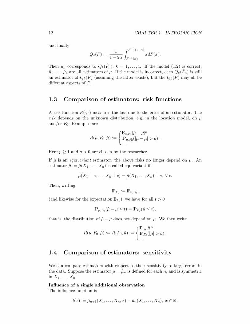
and finally
Q4(F ) :=1
1− 2α
∫ F−1(1−α)
F−1(α)xdF (x).
Then µk corresponds to Qk(Fn), k = 1, . . . , 4. If the model (1.2) is correct,µ1, . . . , µ4 are all estimators of µ. If the model is incorrect, each Qk(Fn) is stillan estimator of Qk(F ) (assuming the latter exists), but the Qk(F ) may all bedifferent aspects of F .
1.3 Comparison of estimators: risk functions
A risk function R(·, ·) measures the loss due to the error of an estimator. Therisk depends on the unknown distribution, e.g. in the location model, on µand/or F0. Examples are
R(µ, F0, µ) :=
IEµ,F0 |µ− µ|pIPµ,F0(|µ− µ| > a). . .
.
Here p ≥ 1 and a > 0 are chosen by the researcher.
If µ is an equivariant estimator, the above risks no longer depend on µ. Anestimator µ := µ(X1, . . . , Xn) is called equivariant if
µ(X1 + c, . . . ,Xn + c) = µ(X1, . . . , Xn) + c, ∀ c.
Then, writingIPF0 := IP0,F0 ,
(and likewise for the expectation IEF0), we have for all t > 0
IPµ,F0(µ− µ ≤ t) = IPF0(µ ≤ t),
that is, the distribution of µ− µ does not depend on µ. We then write
R(µ, F0, µ) := R(F0, µ) :=
IEF0 |µ|pIPF0(|µ| > a). . .
.
1.4 Comparison of estimators: sensitivity
We can compare estimators with respect to their sensitivity to large errors inthe data. Suppose the estimator µ = µn is defined for each n, and is symmetricin X1, . . . , Xn.
Influence of a single additional observationThe influence function is
l(x) := µn+1(X1, . . . , Xn, x)− µn(X1, . . . , Xn), x ∈ R.
1.5. CONFIDENCE INTERVALS 13
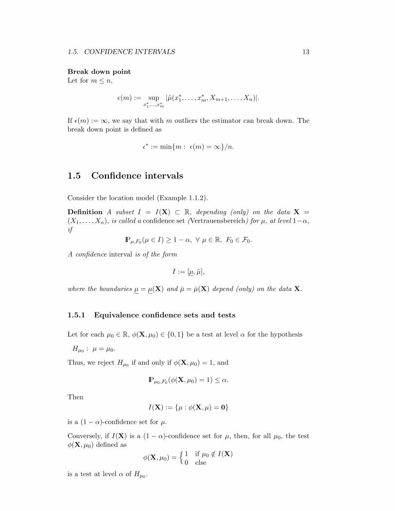
Break down pointLet for m ≤ n,
ε(m) := supx∗1,...,x
∗m
|µ(x∗1, . . . , x∗m, Xm+1, . . . , Xn)|.
If ε(m) :=∞, we say that with m outliers the estimator can break down. Thebreak down point is defined as
ε∗ := minm : ε(m) =∞/n.
1.5 Confidence intervals
Consider the location model (Example 1.1.2).
Definition A subset I = I(X) ⊂ R, depending (only) on the data X =(X1, . . . , Xn), is called a confidence set (Vertrauensbereich) for µ, at level 1−α,if
IPµ,F0(µ ∈ I) ≥ 1− α, ∀ µ ∈ R, F0 ∈ F0.
A confidence interval is of the form
I := [µ, µ],
where the boundaries µ = µ(X) and µ = µ(X) depend (only) on the data X.
1.5.1 Equivalence confidence sets and tests
Let for each µ0 ∈ R, φ(X, µ0) ∈ 0, 1 be a test at level α for the hypothesis
Hµ0 : µ = µ0.
Thus, we reject Hµ0 if and only if φ(X, µ0) = 1, and
IPµ0,F0(φ(X, µ0) = 1) ≤ α.
Then
I(X) := µ : φ(X, µ) = 0
is a (1− α)-confidence set for µ.
Conversely, if I(X) is a (1 − α)-confidence set for µ, then, for all µ0, the testφ(X, µ0) defined as
φ(X, µ0) =
1 if µ0 /∈ I(X)0 else
is a test at level α of Hµ0 .
14 CHAPTER 1. INTRODUCTION
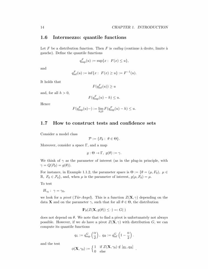
1.6 Intermezzo: quantile functions
Let F be a distribution function. Then F is cadlag (continue a droite, limite agauche). Define the quantile functions
qFsup(u) := supx : F (x) ≤ u,
andqFinf(u) := infx : F (x) ≥ u := F−1(u).
It holds thatF (qFinf(u)) ≥ u
and, for all h > 0,F (qFsup(u)− h) ≤ u.
HenceF (qFsup(u)−) := lim
h↓0F (qFsup(u)− h) ≤ u.
1.7 How to construct tests and confidence sets
Consider a model classP := Pθ : θ ∈ Θ.
Moreover, consider a space Γ, and a map
g : Θ→ Γ, g(θ) := γ.
We think of γ as the parameter of interest (as in the plug-in principle, withγ = Q(Pθ) = g(θ)).
For instance, in Example 1.1.2, the parameter space is Θ := θ = (µ, F0), µ ∈R, F0 ∈ F0, and, when µ is the parameter of interest, g(µ, F0) = µ.
To test
Hγ0 : γ = γ0,
we look for a pivot (Tur-Angel). This is a function Z(X, γ) depending on thedata X and on the parameter γ, such that for all θ ∈ Θ, the distribution
IPθ(Z(X, g(θ)) ≤ ·) =: G(·)
does not depend on θ. We note that to find a pivot is unfortunately not alwayspossible. However, if we do have a pivot Z(X, γ) with distribution G, we cancompute its quantile functions
qL := qGsup
(α2
), qR := qGinf
(1− α
2
).
and the test
φ(X, γ0) :=
1 if Z(X, γ0) /∈ [qL, qR]0 else
.
1.7. HOW TO CONSTRUCT TESTS AND CONFIDENCE SETS 15
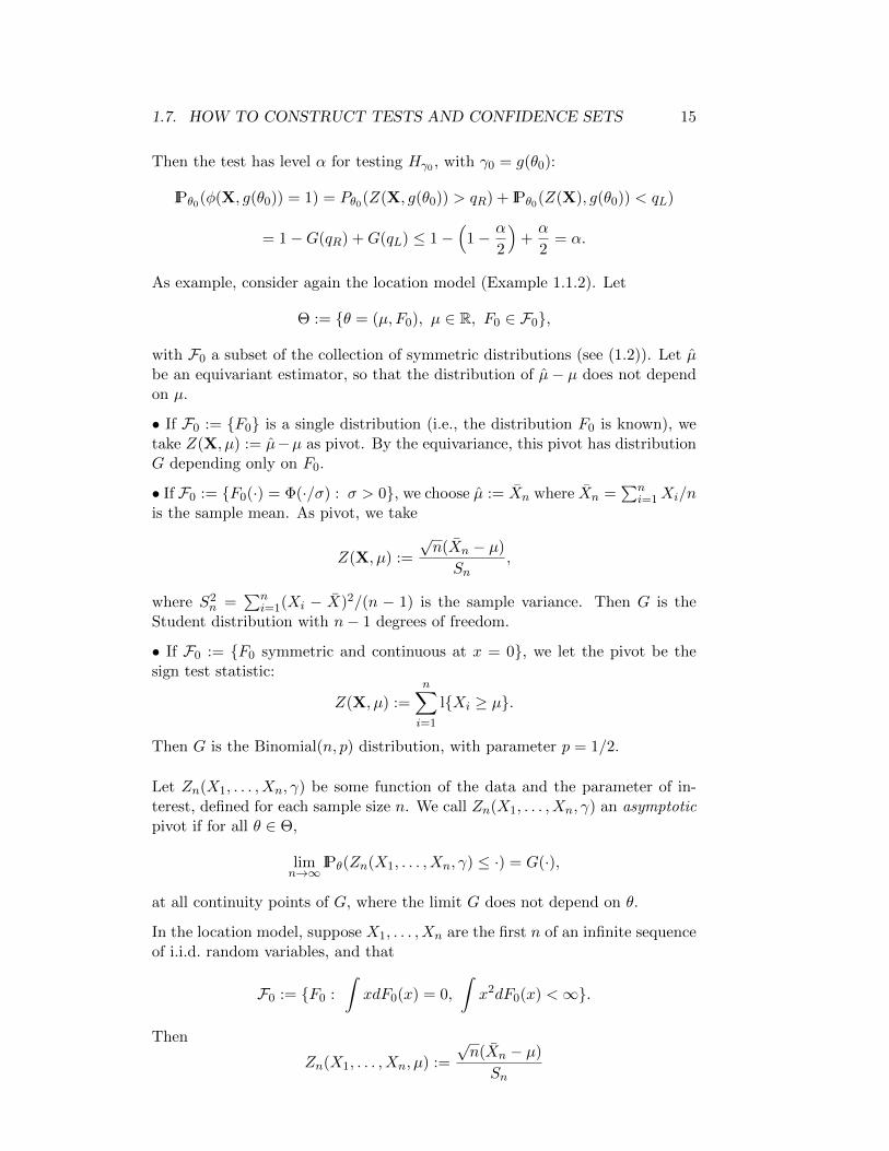
Then the test has level α for testing Hγ0 , with γ0 = g(θ0):
IPθ0(φ(X, g(θ0)) = 1) = Pθ0(Z(X, g(θ0)) > qR) + IPθ0(Z(X), g(θ0)) < qL)
= 1−G(qR) +G(qL) ≤ 1−(
1− α
2
)+α
2= α.
As example, consider again the location model (Example 1.1.2). Let
Θ := θ = (µ, F0), µ ∈ R, F0 ∈ F0,
with F0 a subset of the collection of symmetric distributions (see (1.2)). Let µbe an equivariant estimator, so that the distribution of µ− µ does not dependon µ.
• If F0 := F0 is a single distribution (i.e., the distribution F0 is known), wetake Z(X, µ) := µ−µ as pivot. By the equivariance, this pivot has distributionG depending only on F0.
• If F0 := F0(·) = Φ(·/σ) : σ > 0, we choose µ := Xn where Xn =∑n
i=1Xi/nis the sample mean. As pivot, we take
Z(X, µ) :=
√n(Xn − µ)
Sn,
where S2n =
∑ni=1(Xi − X)2/(n − 1) is the sample variance. Then G is the
Student distribution with n− 1 degrees of freedom.
• If F0 := F0 symmetric and continuous at x = 0, we let the pivot be thesign test statistic:
Z(X, µ) :=n∑i=1
lXi ≥ µ.
Then G is the Binomial(n, p) distribution, with parameter p = 1/2.
Let Zn(X1, . . . , Xn, γ) be some function of the data and the parameter of in-terest, defined for each sample size n. We call Zn(X1, . . . , Xn, γ) an asymptoticpivot if for all θ ∈ Θ,
limn→∞
IPθ(Zn(X1, . . . , Xn, γ) ≤ ·) = G(·),
at all continuity points of G, where the limit G does not depend on θ.
In the location model, suppose X1, . . . , Xn are the first n of an infinite sequenceof i.i.d. random variables, and that
F0 := F0 :
∫xdF0(x) = 0,
∫x2dF0(x) <∞.
Then
Zn(X1, . . . , Xn, µ) :=
√n(Xn − µ)
Sn
16 CHAPTER 1. INTRODUCTION
is an asymptotic pivot, with limiting distribution G = Φ.
Comparison of confidence intervals and testsWhen comparing confidence intervals, the aim is usually to take the one withsmallest length on average (keeping the level at 1 − α). In the case of tests,we look for the one with maximal power. In the location model, this leads tostudying
IEµ,F0 |µ(X)− µ(X)|
for (1 − α)-confidence sets [µ, µ], or to studying the power of test φ(X, µ0) atlevel α. Recall that the power is Pµ,F0(φ(X, µ0) = 1) for values µ 6= µ0.
1.8 An illustration: the two-sample problem
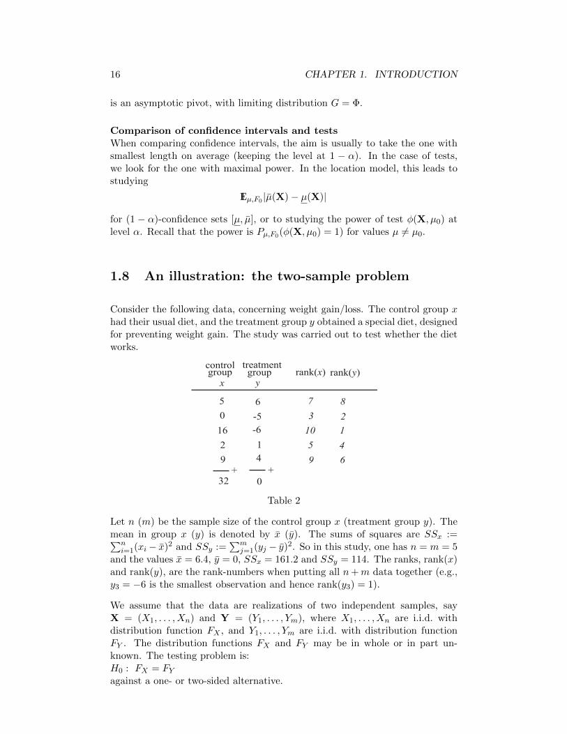
Consider the following data, concerning weight gain/loss. The control group xhad their usual diet, and the treatment group y obtained a special diet, designedfor preventing weight gain. The study was carried out to test whether the dietworks.
controlgroup group
treatment
501629
32+ +
6-5-614
0
rank(x) rank(y)x y
7
9
103
5
82146
Table 2
Let n (m) be the sample size of the control group x (treatment group y). Themean in group x (y) is denoted by x (y). The sums of squares are SSx :=∑n
i=1(xi− x)2 and SSy :=∑m
j=1(yj − y)2. So in this study, one has n = m = 5and the values x = 6.4, y = 0, SSx = 161.2 and SSy = 114. The ranks, rank(x)and rank(y), are the rank-numbers when putting all n+m data together (e.g.,y3 = −6 is the smallest observation and hence rank(y3) = 1).
We assume that the data are realizations of two independent samples, sayX = (X1, . . . , Xn) and Y = (Y1, . . . , Ym), where X1, . . . , Xn are i.i.d. withdistribution function FX , and Y1, . . . , Ym are i.i.d. with distribution functionFY . The distribution functions FX and FY may be in whole or in part un-known. The testing problem is:H0 : FX = FYagainst a one- or two-sided alternative.
1.8. AN ILLUSTRATION: THE TWO-SAMPLE PROBLEM 17
1.8.1 Assuming normality
The classical two-sample student test is based on the assumption that the datacome from a normal distribution. Moreover, it is assumed that the variance ofFX and FY are equal. Thus,
(FX , FY ) ∈FX = Φ
(· − µσ
), FY = Φ
(· − (µ+ γ)
σ
): µ ∈ R, σ > 0, γ ∈ Γ
.
Here, Γ ⊃ 0 is the range of shifts in mean one considers, e.g. Γ = R fortwo-sided situations, and Γ = (−∞, 0] for a one-sided situation. The testingproblem reduces toH0 : γ = 0.
We now look for a pivot Z(X,Y, γ). Define the sample means
X :=1
n
n∑i=1
Xi, Y :=1
m
m∑j=1
Yj ,
and the pooled sample variance
S2 :=1
m+ n− 2
n∑i=1
(Xi − X)2 +m∑j=1
(Yj − Y )2
.
Note that X has expectation µ and variance σ2/n, and Y has expectation µ+γand variance σ2/m. So Y − X has expectation γ and variance
σ2
n+σ2
m= σ2
(n+m
nm
).
The normality assumption implies that
Y − X is N(γ, σ2
(n+m
nm
))−distributed.
Hence √nm
n+m
(Y − X − γ
σ
)is N (0, 1)−distributed.
To arrive at a pivot, we now plug in the estimate S for the unknown σ:
Z(X,Y, γ) :=
√nm
n+m
(Y − X − γ
S
).
Indeed, Z(X,Y, γ) has a distribution G which does not depend on unknownparameters. The distribution G is Student(n+m−2) (the Student-distributionwith n+m−2 degrees of freedom). As test statistic for H0 : γ = 0, we thereforetake
T = T Student := Z(X,Y, 0).
18 CHAPTER 1. INTRODUCTION
The one-sided test at level α, for H0 : γ = 0 against H1 : γ < 0, is
φ(X,Y) :=
1 if T < −tn+m−2(1− α)0 if T ≥ −tn+m−2(1− α)
,
where, for ν > 0, tν(1− α) = −tν(α) is the (1− α)-quantile of the Student(ν)-distribution.
Let us apply this test to the data given in Table 2. We take α = 0.05. Theobserved values are x = 6.4, y = 0 and s2 = 34.4. The test statistic takes thevalue −1.725 which is bigger than the 5% quantile t8(0.05) = −1.9. Hence, wecannot reject H0. The p-value of the observed value of T is
p−value := IPγ=0(T < −1.725) = 0.06.
So the p-value is in this case only a little larger than the level α = 0.05.
1.8.2 A nonparametric test
In this subsection, we suppose that FX and FY are continuous, but otherwiseunknown. The model class for both FX and FY is thus
F := all continuous distributions.
The continuity assumption ensures that all observations are distinct, that is,there are no ties. We can then put them in strictly increasing order. LetN = n+m and Z1, . . . , ZN be the pooled sample
Zi := Xi, i = 1, . . . , n, Zn+j := Yj , j = 1, . . . ,m.
Define
Ri := rank(Zi), i = 1, . . . , N.
and let
Z(1) < · · · < Z(N)
be the order statistics of the pooled sample (so that Zi = Z(Ri) (i = 1, . . . , n)).The Wilcoxon test statistic is
T = TWilcoxon :=n∑i=1
Ri.
One may check that this test statistic T can alternatively be written as
T = #Yj < Xi+n(n+ 1)
2.
For example, for the data in Table 2, the observed value of T is 34, and
#yj < xi = 19,n(n+ 1)
2= 15.
1.8. AN ILLUSTRATION: THE TWO-SAMPLE PROBLEM 19
Large values of T mean that the Xi are generally larger than the Yj , and henceindicate evidence against H0.
To check whether or not the observed value of the test statistic is compatiblewith the null-hypothesis, we need to know its null-distribution, that is, thedistribution under H0. Under H0 : FX = FY , the vector of ranks (R1, . . . , Rn)has the same distribution as n random draws without replacement from thenumbers 1, . . . , N. That is, if we let
r := (r1, . . . , rn, rn+1, . . . , rN )
denote a permutation of 1, . . . , N, then
IPH0
((R1, . . . , Rn, Rn+1, . . . RN ) = r
)=
1
N !,
(see Theorem 1.8.1), and hence
IPH0(T = t) =#r :
∑ni=1 ri = tN !
.
This can also be written as
IPH0(T = t) =1(Nn
)#r1 < · · · < rn < rn+1 < · · · < rN :n∑i=1
ri = t.
So clearly, the null-distribution of T does not depend on FX or FY . It doeshowever depend on the sample sizes n and m. It is tabulated for n and msmall or moderately large. For large n and m, a normal approximation of thenull-distribution can be used.
Theorem 1.8.1 formally derives the null-distribution of the test, and actuallyproves that the order statistics and the ranks are independent. The latter resultwill be of interest in Example 2.10.4.
For two random variables X and Y , use the notation
XD= Y
when X and Y have the same distribution.
Theorem 1.8.1 Let Z1, . . . , ZN be i.i.d. with continuous distribution F onR. Then (Z(1), . . . , Z(N)) and R := (R1, . . . , RN ) are independent, and for allpermutations r := (r1, . . . , rN ),
IP(R = r) =1
N !.
Proof. Let ZQi := Z(i), and Q := (Q1, . . . , QN ). Then
R = r ⇔ Q = r−1 := q,
20 CHAPTER 1. INTRODUCTION
where r−1 is the inverse permutation of r.1 For all permutations q and allmeasurable maps f ,
f(Z1, . . . , ZN )D= f(Zq1 , . . . , ZqN ).
Therefore, for all measurable sets A ⊂ RN , and all permutations q,
IP
((Z1, . . . , ZN ) ∈ A, Z1 < . . . < ZN
)
= IP
((Zq1 . . . , ZqN ) ∈ A, Zq1 < . . . < ZqN
).
Because there are N ! permutations, we see that for any q,
IP
((Z(1), . . . , Z(n)) ∈ A
)= N !IP
((Zq1 . . . , ZqN ) ∈ A, Zq1 < . . . < ZqN
)
= N !IP
((Z(1), . . . , Z(N)) ∈ A, R = r
),
where r = q−1. Thus we have shown that for all measurable A, and for all r,
IP
((Z(1), . . . , Z(N)) ∈ A, R = r
)=
1
N !IP
((Z(1), . . . , Z(n)) ∈ A
). (1.5)
Take A = RN to find that (1.5) implies
IP
(R = r
)=
1
N !.
Plug this back into (1.5) to see that we have the product structure
IP
((Z(1), . . . , Z(N)) ∈ A, R = r
)= IP
((Z(1), . . . , Z(n)) ∈ A
)IP
(R = r
),
which holds for all measurable A. In other words, (Z(1), . . . , Z(N)) and R areindependent. tu
1.8.3 Comparison of Student’s test and Wilcoxon’s test
Because Wilcoxon’s test is ony based on the ranks, and does not rely on theassumption of normality, it lies at hand that, when the data are in fact normallydistributed, Wilcoxon’s test will have less power than Student’s test. The loss
1Here is an example, with N = 3:
(z1, z2, z3) = ( 5 , 6 , 4 )
(r1, r2, r3) = ( 2 , 3 , 1 )
(q1, q2, q3) = ( 3 , 1 , 2 )
1.9. HOW TO CONSTRUCT ESTIMATORS 21
of power is however small. Let us formulate this more precisely, in terms ofthe relative efficiency of the two tests. Let the significance α be fixed, andlet β be the required power. Let n and m be equal, N = 2n be the totalsample size, and NStudent (NWilcoxon) be the number of observations needed toreach power β using Student’s (Wilcoxon’s) test. Consider shift alternatives,i.e. FY (·) = FX(· − γ), (with, in our example, γ < 0). One can show thatNStudent/NWilcoxon is approximately .95 when the normal model is correct. Fora large class of distributions, the ratio NStudent/NWilcoxon ranges from .85 to∞,that is, when using Wilcoxon one generally has very limited loss of efficiency ascompared to Student, and one may in fact have a substantial gain of efficiency.
1.9 How to construct estimators
Consider i.i.d. observations X1, . . . , Xn, copies of a random variable X withdistribution P ∈ Pθ : θ ∈ Θ. The parameter of interest is denoted byγ = g(θ) ∈ Γ.
1.9.1 Plug-in estimators
For real-valued observations, one can define the distribution function
F (·) = P (X ≤ ·).
An estimator of F is the empirical distribution function
Fn(·) =1
n
n∑i=1
lXi ≤ ·.
Note that when knowing only Fn, one can reconstruct the order statisticsX(1) ≤ . . . ≤ X(n), but not the original data X1, . . . , Xn. Now, the orderat which the data are given carries no information about the distribution P . Inother words, a “reasonable”2 estimator T = T (X1, . . . , Xn) depends only on thesample (X1, . . . , Xn) via the order statistics (X(1), . . . X(n)) (i.e., shuffling thedata should have no influence on the value of T ). Because these order statisticscan be determined from the empirical distribution Fn, we conclude that any“reasonable” estimator T can be written as a function of Fn:
T = Q(Fn),
for some map Q.
Similarly, the distribution function Fθ := Pθ(X ≤ ·) completely characterizesthe distribution P . Hence, a parameter is a function of Fθ:
γ = g(θ) = Q(Fθ).
2What is “reasonable” has to be considered with some care. There are in fact “reasonable”statistical procedures that do treat the Xi in an asymmetric way. An example is splittingthe sample into a training and test set (for model validation).
22 CHAPTER 1. INTRODUCTION
If the mapping Q is defined at all Fθ as well as at Fn, we call Q(Fn) a plug-inestimator of Q(Fθ).
The idea is not restricted to the one-dimensional setting. For arbitrary obser-vation space X , we define the empirical measure
Pn =1
n
n∑i=1
δXi ,
where δx is a point-mass at x. The empirical measure puts mass 1/n at eachobservation. This is indeed an extension of X = R to general X , as the empiricaldistribution function Fn jumps at each observation, with jump height equal tothe number of times the value was observed (i.e. jump height 1/n if all Xi aredistinct). So, as in the real-valued case, if the map Q is defined at all Pθ as wellas at Pn, we call Q(Pn) a plug-in estimator of Q(Pθ).
We stress that typically, the representation γ = g(θ) as function Q of Pθ is notunique, i.e., that there are various choices of Q. Each such choice generallyleads to a different estimator. Moreover, the assumption that Q is defined atPn is often violated. One can sometimes modify the map Q to a map Qn that,in some sense, approximates Q for n large. The modified plug-in estimator thentakes the form Qn(Pn).
1.9.2 The method of moments
Let X ∈ R and suppose (say) that the parameter of interest is θ itself, andthat Θ ⊂ Rp. Let µ1(θ), . . . , µp(θ) denote the first p moments of X (assumedto exist), i.e.,
µj(θ) = EθXj =
∫xjdFθ(x), j = 1, . . . , p.
Also assume that the mapm : Θ→ Rp,
defined bym(θ) = [µ1(θ), . . . , µp(θ)],
has an inversem−1(µ1, . . . , µp),
for all [µ1, . . . , µp] ∈M (say). We estimate the µj by their sample counterparts
µj :=1
n
n∑i=1
Xji =
∫xjdFn(x), j = 1, . . . , p.
When [µ1, . . . , µp] ∈M we can plug them in to obtain the estimator
θ := m−1(µ1, . . . , µp).
Example
1.9. HOW TO CONSTRUCT ESTIMATORS 23
Let X have the negative binomial distribution with known parameter k andunknown success parameter θ ∈ (0, 1):
Pθ(X = x) =
(k + x− 1
x
)θk(1− θ)x, x ∈ 0, 1, . . ..
This is the distribution of the number of failures till the kth success, where ateach trial, the probability of success is θ, and where the trials are independent.It holds that
Eθ(X) = k(1− θ)θ
:= m(θ).
Hence
m−1(µ) =k
µ+ k,
and the method of moments estimator is
θ =k
X + k=
nk∑ni=1Xi + nk
=number of successes
number of trails.
Example
Suppose X has density
pθ(x) = θ(1 + x)−(1+θ), x > 0,
with respect to Lebesgue measure, and with θ ∈ Θ ⊂ (0,∞). Then, for θ > 1
EθX =1
θ − 1:= m(θ),
with inverse
m−1(µ) =1 + µ
µ.
The method of moments estimator would thus be
θ =1 + X
X.
However, the mean EθX does not exist for θ < 1, so when Θ contains valuesθ < 1, the method of moments is perhaps not a good idea. We will see that themaximum likelihood estimator does not suffer from this problem.
1.9.3 Likelihood methods
Suppose that P := Pθ : θ ∈ Θ is dominated by a σ-finite measure ν. Wewrite the densities as
pθ :=dPθdν
, θ ∈ Θ.
Definition The likelihood function (of the data X = (X1, . . . , Xn)) is
LX(ϑ) :=
n∏i=1
pϑ(Xi).
24 CHAPTER 1. INTRODUCTION
The MLE (maximum likelihood estimator) is
θ := arg maxϑ∈Θ
LX(ϑ).
Note We use the symbol ϑ for the variable in the likelihood function, and theslightly different symbol θ for the parameter we want to estimate. It is howevera common convention to use the same symbol for both (as already noted in theearlier section on estimation). However, as we will see below, different symbolsare needed for the development of the theory.
Note Alternatively, we may write the MLE as the maximizer of the log-likelihood
θ = arg maxϑ∈Θ
logLX(ϑ) = arg maxϑ∈Θ
n∑i=1
log pϑ(Xi).
The log-likelihood is generally mathematically more tractable. For example,if the densities are differentiable, one can typically obtain the maximum bysetting the derivatives to zero, and it is easier to differentiate a sum than aproduct.
Note The likelihood function may have local maxima. Moreover, the MLE isnot always unique, or may not exist (for example, the likelihood function maybe unbounded).
We will now show that maximum likelihood is a plug-in method. First, as notedabove, the MLE maximizes the log-likelihood. We may of course normalize thelog-likelihood by 1/n:
θ = arg maxϑ∈Θ
1
n
n∑i=1
log pϑ(Xi).
Replacing the average∑n
i=1 log pϑ(Xi)/n by its theoretical counterpart gives
arg maxϑ∈Θ
Eθ log pϑ(X)
which is indeed equal to the parameter θ we are trying to estimate: by theinequality log x ≤ x− 1, x > 0,
Eθ logpϑ(X)
pθ(X)≤ Eθ
(pϑ(X)
pθ(X)− 1
)= 0.
(Note that using different symbols ϑ and θ is indeed crucial here.) Chapter 6will put this is a wider perspective.
Example
We turn back to the previous example. Suppose X has density
pθ(x) = θ(1 + x)−(1+θ), x > 0,
1.9. HOW TO CONSTRUCT ESTIMATORS 25
with respect to Lebesgue measure, and with θ ∈ Θ = (0,∞). Then
log pϑ(x) = log ϑ− (1 + ϑ) log(1 + x),
d
dϑlog pϑ(x) =
1
ϑ− log(1 + x).
We put the derivative of the log-likelihood to zero and solve:
n
θ−
n∑i=1
log(1 +Xi) = 0
⇒ θ =1
∑n
i=1 log(1 +Xi)/n.
(One may check that this is indeed the maximum.)
Example
Let X ∈ R and θ = (µ, σ2), with µ ∈ R a location parameter, σ > 0 a scaleparameter. We assume that the distribution function Fθ of X is
Fθ(·) = F0
(· − µσ
),
where F0 is a given distribution function, with density f0 w.r.t. Lebesgue mea-sure. The density of X is thus
pθ(·) =1
σf0
(· − µσ
).
Case 1 If F0 = Φ (the standard normal distribution), then
f0(x) = φ(x) =1√2π
exp
[−1
2x2
], x ∈ R,
so that
pθ(x) =1√
2πσ2exp
[− 1
2σ2(x− µ)2
], x ∈ R.
The MLE of µ resp. σ2 is
µ = X, σ2 =1
n
n∑i=1
(Xi − X)2.
Case 2 The (standardized) double exponential or Laplace distribution has den-sity
f0(x) =1√2
exp
[−√
2|x|], x ∈ R,
so
pθ(x) =1√2σ2
exp
[−√
2|x− µ|σ
], x ∈ R.
26 CHAPTER 1. INTRODUCTION
The MLE of µ resp. σ is now
µ = sample median, σ =
√2
n
n∑i=1
|Xi − µ2|.
Example
Here is a famous example, from Kiefer and Wolfowitz (1956), where the like-lihood is unbounded, and hence the MLE does not exist. It concerns the caseof a mixture of two normals: each observation, is either N (µ, 1)-distributed orN (µ, σ2)-distributed, each with probability 1/2 (say). The unknown parameteris θ = (µ, σ2), and X has density
pθ(x) =1
2φ(x− µ) +
1
2σφ((x− µ)/σ), x ∈ R,
w.r.t. Lebesgue measure. Then
LX(µ, σ2) =n∏i=1
(1
2φ(Xi − µ) +
1
2σφ((Xi − µ)/σ)
).
Taking µ = X1 yields
LX(X1, σ2) =
1√2π
(1
2+
1
2σ)n∏i=2
(1
2φ(Xi −X1) +
1
2σφ((Xi −X1)/σ)
).
Now, since for all z 6= 0
limσ↓0
1
σφ(z/σ) = 0,
we have
limσ↓0
n∏i=2
(1
2φ(Xi −X1) +
1
2σφ((Xi −X1)/σ)
)=
n∏i=2
1
2φ(Xi −X1) > 0.
It follows that
limσ↓0
LX(X1, σ2) =∞.
Asymptotic tests and confidence intervals based on the likelihood
Suppose that Θ is an open subset of Rp. Define the log-likelihood ratio
Z(X, θ) := 2
logLX(θ)− logLX(θ)
.
Note that Z(X, θ) ≥ 0, as θ maximizes the (log)-likelihood. We will see inChapter 6 that, under some regularity conditions,
Z(X, θ)Dθ−→ χ2
p, ∀ θ.
1.9. HOW TO CONSTRUCT ESTIMATORS 27
Here, “Dθ−→ ” means convergence in distribution under IPθ, and χ2
p denotes theChi-squared distribution with p degrees of freedom.
Thus, Z(X, θ) is an asymptotic pivot. For the null-hypotheses
H0 : θ = θ0,
a test at asymptotic level α is: reject H0 if Z(X, θ0) > χ2p(1−α), where χ2
p(1−α)is the (1−α)-quantile of the χ2
p-distribution. An asymptotic (1−α)-confidenceset for θ is
θ : Z(X, θ) ≤ χ2p(1− α)
= θ : 2 logLX(θ) ≤ 2 logLX(θ) + χ2p(1− α).
Example
Here is a toy example. Let X have the N (µ, 1)-distribution, with µ ∈ R un-known. The MLE of µ is the sample average µ = X. It holds that
logLX(µ) = −n2
log(2π)− 1
2
n∑i=1
(Xi − X)2,
and
2
logLX(µ)− logLX(µ)
= n(X − µ)2.
The random variable√n(X−µ) is N (0, 1)-distributed under IPµ. So its square,
n(X − µ)2, has a χ21-distribution. Thus, in this case the above test (confidence
interval) is exact.

28 CHAPTER 1. INTRODUCTION
Chapter 2
Decision theory
NotationIn this chapter, we denote the observable random variable (the data) by X ∈ X ,and its distribution by P ∈ P. The probability model is P := Pθ : θ ∈ Θ,with θ an unknown parameter. In particular cases, we apply the results withX being replaced by a vector X = (X1, . . . , Xn), with X1, . . . , Xn i.i.d. withdistribution P ∈ Pθ : θ ∈ Θ (so that X has distribution IP :=
∏ni=1 P ∈
IPθ =∏ni=1 Pθ : θ ∈ Θ).
2.1 Decisions and their risk
Let A be the action space.
• A = R corresponds to estimating a real-valued parameter.
• A = 0, 1 corresponds to testing a hypothesis.
• A = [0, 1] corresponds to randomized tests.
• A = intervals corresponds to confidence intervals.
Given the observation X, we decide to take a certain action in A. Thus, anaction is a map d : X → A, with d(X) being the decision taken.
A loss function (Verlustfunktion) is a map
L : Θ×A → R,
with L(θ, a) being the loss when the parameter value is θ and one takes actiona.
The risk of decision d(X) is defined as
R(θ, d) := EθL(θ, d(X)), θ ∈ Θ.
29
30 CHAPTER 2. DECISION THEORY
Example 2.1.1 In the case of estimating a parameter of interest g(θ) ∈ R, theaction space is A = R (or a subset thereof). Important loss functions are then
L(θ, a) := w(θ)|g(θ)− a|r,
where w(·) are given non-negative weights and r ≥ 0 is a given power. The riskis then
R(θ, d) = w(θ)Eθ|g(θ)− d(X)|r.
A special case is taking w ≡ 1 and r = 2. Then
R(θ, d) = Eθ|g(θ)− d(X)|2
is called the mean square error.
Example 2.1.2 Consider testing the hypothesis
H0 : θ ∈ Θ0
against the alternative
H1 : θ ∈ Θ1.
Here, Θ0 and Θ1 are given subsets of Θ with Θ0 ∩Θ1 = ∅. As action space, wetake A = 0, 1, and as loss
L(θ, a) :=
1 if θ ∈ Θ0 and a = 1c if θ ∈ Θ1 and a = 00 otherwise
.
Here c > 0 is some given constant. Then
R(θ, d) =
Pθ(d(X) = 1) if θ ∈ Θ0
cPθ(d(X) = 0) if θ ∈ Θ1
0 otherwise
.
Thus, the risks correspond to the error probabilities (type I and type II errors).
NoteThe best decision d is the one with the smallest risk R(θ, d). However, θ is notknown. Thus, if we compare two decision functions d1 and d2, we may run intoproblems because the risks are not comparable: R(θ, d1) may be smaller thanR(θ, d2) for some values of θ, and larger than R(θ, d2) for other values of θ.
Example 2.1.3 Let X ∈ R and let g(θ) = EθX := µ. We take quadratic loss
L(θ, a) := |µ− a|2.
Assume that varθ(X) = 1 for all θ. Consider the collection of decisions
dλ(X) := λX,
where 0 ≤ λ ≤ 1. Then
R(θ, dλ) = var(λX) + bias2θ(λX)
2.2. ADMISSIBILITY 31
= λ2 + (λ− 1)2µ2.
The “optimal” choice for λ would be
λopt :=µ2
1 + µ2,
because this value minimizes R(θ, dλ). However, λopt depends on the unknownµ, so dλopt(X) is not an estimator.
Various optimality conceptsWe will consider three optimality concepts: admissibility (zulassigkeit), mini-max and Bayes.
2.2 Admissibility
Definition A decision d′ is called strictly better than d if
R(θ, d′) ≤ R(θ, d), ∀ θ,
and
∃ θ : R(θ, d′) < R(θ, d).
When there exists a d′ that is strictly better than d, then d is called inadmissible.
Example 2.2.1 Let, for n ≥ 2, X1, . . . , Xn be i.i.d., with g(θ) := Eθ(Xi) := µ,and var(Xi) = 1 (for all i). Take quadratic loss L(θ, a) := |µ − a|2. Considerd′(X1, . . . , Xn) := Xn and d(X1, . . . , Xn) := X1. Then, ∀ θ,
R(θ, d′) =1
n, R(θ, d) = 1,
so that d is inadmissible.
NoteWe note that to show that a decision d is inadmissible, it suffices to find astrictly better d′. On the other hand, to show that d is admissible, one has toverify that there is no strictly better d′. So in principle, one then has to takeall possible d′ into account.
Example 2.2.2 Let L(θ, a) := |g(θ)− a|r and d(X) := g(θ0), where θ0 is somefixed given value.
Lemma Assume that Pθ0 dominates Pθ1 for all θ. Then d is admissible.
Proof.
1Let P and Q be probability measures on the same measurable space. Then P dominatesQ if for all measurable B, P (B) = 0 implies Q(B) = 0 (Q is absolut stetig bezuglich P ).
32 CHAPTER 2. DECISION THEORY
Suppose that d′ is better than d. Then we have
Eθ0 |g(θ0)− d′(X)|r ≤ 0.
This implies that
d′(X) = g(θ0), Pθ0−almost surely. (2.1)
Since by (2.1),
Pθ0(d′(X) 6= g(θ0)) = 0
the assumption that Pθ0 dominates Pθ, ∀ θ, implies now
Pθ(d′(X) 6= g(θ0)) = 0, ∀ θ.
That is, for all θ, d′(X) = g(θ0), Pθ-almost surely, and hence, for all θ, R(θ, d′) =R(θ, d). So d′ is not strictly better than d. We conclude that d is admissible. tu
Example 2.2.3 We consider testing
H0 : θ = θ0
against the alternative
H1 : θ = θ1.
We let A = [0, 1] and let d := φ be a randomized test. As risk, we take
R(θ, φ) :=
Eθφ(X), θ = θ0
1− Eθφ(X), θ = θ1.
We let p0 (p1) be the density of Pθ0 (Pθ1) with respect to some dominatingmeasure ν (for example ν = Pθ0 + Pθ1). A Neyman Pearson test is
φNP :=
1 if p1/p0 > cq if p1/p0 = c0 if p1/p0 < c
.
Here 0 ≤ q ≤ 1, and 0 ≤ c < ∞ are given constants. To check whether φNP isadmissible, we first recall the Neyman Pearson Lemma.
Neyman Pearson Lemma Let φ be some test. We have
R(θ1, φNP)−R(θ1, φ) ≤ c[R(θ0, φ)−R(θ0, φNP)].
Proof.
R(θ1, φNP)−R(θ1, φ) =
∫(φ− φNP)p1
=
∫p1/p0>c
(φ− φNP)p1 +
∫p1/p0=c
(φ− φNP)p1 +
∫p1/p0<c
(φ− φNP)p1
≤ c∫p1/p0>c
(φ− φNP)p0 + c
∫p1/p0=c
(φ− φNP)p0 + c
∫p1/p0<c
(φ− φNP)p0
2.3. MINIMAXITY 33
= c[R(θ0, φ)−R(θ0, φNP)].
tu
Lemma A Neyman Pearson test is admissible if and only if one of the followingtwo cases hold:i) its power is strictly less than 1,orii) it has minimal level among all tests with power 1.
Proof. Suppose R(θ0, φ) < R(θ0, φNP). Then from the Neyman PearsonLemma, we know that either R(θ1, φ) > R(θ1, φNP) (i.e., then φ is not bet-ter then φNP), or c = 0. But when c = 0, it holds that R(θ1, φNP) = 0, i.e. thenφNP has power one.
Similarly, suppose that R(θ1, φ) < R(θ1, φNP). Then it follows from the NeymanPearson Lemma that R(θ0, φ) > R(θ0, φNP), because we assume c <∞.
tu
2.3 Minimaxity
Definition A decision d is called minimax if
supθR(θ, d) = inf
d′supθR(θ, d′).
Thus, the minimax criterion concerns the best decision in the worst possiblecase.
Lemma A Neyman Pearson test φNP is minimax, if and only if R(θ0, φNP) =R(θ1, φNP).
Proof. Let φ be a test, and write for j = 0, 1,
rj := R(θj , φNP), r′j = R(θj , φ).
Suppose that r0 = r1 and that φNP is not minimax. Then, for some test φ,
maxjr′j < max
jrj .
This implies that bothr′0 < r0, r
′1 < r1
and by the Neyman Pearson Lemma, this is not possible.
Let S = (R(θ0, φ), R(θ1, φ)) : φ : X → [0, 1]. Note that S is convex. Thus, ifr0 < r1, we can find a test φ with r0 < r′0 < r1 and r′1 < r1. So then φNP is notminimax. Similarly if r0 > r1.
tu
34 CHAPTER 2. DECISION THEORY
2.4 Bayes decisions
Suppose the parameter space Θ is a measurable space. We can then equip itwith a probability measure Π. We call Π the a priori distribution.
Definition The Bayes risk (with respect to the probability measure Π) is
r(Π, d) :=
∫ΘR(ϑ, d)dΠ(ϑ).
A decision d is called Bayes (with respect to Π) if
r(Π, d) = infd′r(Π, d′).
If Π has density w := dΠ/dµ with respect to some dominating measure µ, wemay write
r(Π, d) =
∫ΘR(ϑ, d)w(ϑ)dµ(ϑ) := rw(d).
Thus, the Bayes risk may be thought of as taking a weighted average of therisks. For example, one may want to assign more weight to “important” valuesof θ.
Example 2.4.1 Consider again the testing problem
H0 : θ = θ0
against the alternative
H1 : θ = θ1.
Let L(θ0, a) := a and L(θ1, a) := 1− a, w(θ0) =: w0 and w(θ1) =: w1 = 1−w0.Then
rw(φ) := w0R(θ0, φ) + w1R(θ1, φ).
We take 0 < w0 = 1− w1 < 1.
Lemma Bayes test is
φBayes =
1 if p1/p0 > w0/w1
q if p1/p0 = w0/w1
0 if p1/p0 < w0/w1
.
Proof.
rw(φ) = w0
∫φp0 + w1(1−
∫φp1)
=
∫φ(w0p0 − w1p1) + w1.
So we choose φ ∈ [0, 1] to minimize φ(w0p0 − w1p1). This is done by taking
φ =
1 if w0p0 − w1p1 < 0q if w0p0 − w1p1 = 00 if w0p0 − w1p1 > 0
,
2.5. INTERMEZZO: CONDITIONAL DISTRIBUTIONS 35
where for q we may take any value between 0 and 1. tu
Note that
2rw(φBayes) = 1−∫|w1p1 − w0p0|.
In particular, when w0 = w1 = 1/2,
2rw(φBayes) = 1−∫|p1 − p0|/2,
i.e., the risk is large if the two densities are close to each other.
2.5 Intermezzo: conditional distributions
Recall the definition of conditional probabilities: for two sets A and B, withP (B) 6= 0, the conditional probability of A given B is defined as
P (A|B) =P (A ∩B)
P (B).
It follows that
P (B|A) = P (A|B)P (B)
P (A),
and that, for a partition Bj2
P (A) =∑j
P (A|Bj)P (Bj).
Consider now two random vectors X ∈ Rn and Y ∈ Rm. Let fX,Y (·, ·), be thedensity of (X,Y ) with respect to Lebesgue measure (assumed to exist). Themarginal density of X is
fX(·) =
∫fX,Y (·, y)dy,
and the marginal density of Y is
fY (·) =
∫fX,Y (x, ·)dx.
Definition The conditional density of X given Y = y is
fX(x|y) :=fX,Y (x, y)
fY (y), x ∈ Rn.
2Bj is a partition if Bj ∩Bk = ∅ for all j 6= k and P (∪jBj) = 1.
36 CHAPTER 2. DECISION THEORY
Thus, we have
fY (y|x) = fX(x|y)fY (y)
fX(x), (x, y) ∈ Rn+m,
and
fX(x) =
∫fX(x|y)fY (y)dy, x ∈ Rn.
Definition The conditional expectation of g(X,Y ) given Y = y is
E[g(X,Y )|Y = y] :=
∫fX(x|y)g(x, y)dx.
Note thus that
E[g1(X)g2(Y )|Y = y] = g2(y)E[g1(X)|Y = y].
Notation We define the random variable E[g(X,Y )|Y ] as
E[g(X,Y )|Y ] := h(Y ),
where h(y) is the function h(y) := E[g(X,Y )|Y = y].
Lemma 2.5.1 (Iterated expectations lemma) It holds that
E
[[E[g(X,Y )|Y ]
]= Eg(X,Y ).
Proof. Define
h(y) := E[g(X,Y )|Y = y].
Then
Eh(Y ) =
∫h(y)fY (y)dy =
∫E[g(X,Y )|Y = y]fY (y)dy
=
∫ ∫g(x, y)fX,Y (x, y)dxdy = Eg(X,Y ).
tu
2.6 Bayes methods
Let X have distribution P ∈ P := Pθ : θ ∈ Θ. Suppose P is dominated by a(σ-finite) measure ν, and let pθ = dPθ/dν denote the densities. Let Π be an apriori distribution on Θ, with density w := dΠ/dµ. We now think of pθ as thedensity of X given the value of θ. We write it as
pθ(x) = p(x|θ), x ∈ X .
2.6. BAYES METHODS 37
Moreover, we define
p(·) :=
∫Θp(·|ϑ)w(ϑ)dµ(ϑ).
Definition The a posteriori density of θ is
w(ϑ|x) = p(x|ϑ)w(ϑ)
p(x), ϑ ∈ Θ, x ∈ X .
Lemma 2.6.1 Given the data X = x, consider θ as a random variable withdensity w(ϑ|x). Let
l(x, a) := E[L(θ, a)|X = x] =
∫ΘL(ϑ, a)w(ϑ|x)dµ(ϑ),
andd(x) := arg min
al(x, a).
Then d is Bayes decision dBayes.
Proof.
rw(d′) =
∫ΘR(ϑ, d′)w(ϑ)dµ(ϑ)
=
∫Θ
[∫XL(ϑ, d′(x))p(x|ϑ)dν(x)
]w(ϑ)dµ(ϑ)
=
∫X
[∫ΘL(ϑ, d′(x))w(ϑ|x)dµ(ϑ)
]p(x)dν(x)
=
∫Xl(x, d′(x))p(x)dν(x)
≥∫Xl(x, d(x))p(x)dν(x)
= rw(d).
tu
Example 2.6.1 For the testing problem
H0 : θ = θ0
against the alternative
H1 : θ = θ1, with loss function
L(θ0, a) := a, L(θ1, a) := 1− a, a ∈ 0, 1,
we havel(x, φ) = φw0p0(x)/p(x) + (1− φ)w1p1(x)/p(x).
Thus,
arg minφl(·, φ) =
1 if w1p1 > w0p0
q if w1p1 = w0p0
0 if w1p1 < w0p0
.
38 CHAPTER 2. DECISION THEORY
In the next example, we shall use:
Lemma. Let Z be a real-valued random variable. Then
arg mina∈R
E(Z − a)2 = EZ.
Proof.
E(Z − a)2 = var(Z) + (a− EZ)2.
tu
Example 2.6.2 Consider the case A = R and Θ ⊆ R . Let L(θ, a) := |θ− a|2.Then
dBayes(X) = E(θ|X).
Example 2.6.3 Consider again the case Θ ⊆ R, and A = Θ, and now withloss function L(θ, a) := l|θ − a| > c for a given constant c > 0. Then
l(x, a) = Π(|θ − a| > c|X = x) =
∫|ϑ−a|>c
w(ϑ|x)dϑ.
We note that for c→ 0
1− l(x, a)
2c=
Π(|θ − a| ≤ c|X = x)
2c≈ w(a|x) = p(x|a)
w(a)
p(x).
Thus, for c small, Bayes rule is approximately d0(x) := arg maxa∈Θ p(x|a)w(a).The estimator d0(X) is called the maximum a posteriori estimator. If w is theuniform density on Θ (which only exists if Θ is bounded), then d0(X) is themaximum likelihood estimator.
Example 2.6.4 Suppose that given θ, X has Poisson distribution with pa-rameter θ, and that θ has the Gamma(k, λ)-distribution. The density of θ isthen
w(ϑ) = λkϑk−1e−λϑ/Γ(k),
where
Γ(k) =
∫ ∞0
e−zzk−1dz.
The Gamma(k, λ) distribution has mean
Eθ =
∫ ∞0
ϑw(ϑ)dϑ =k
λ.
The a posteriori density is then
w(ϑ|x) = p(x|ϑ)w(ϑ)
p(x)
= e−ϑϑx
x!
λkϑk−1e−λϑ/Γ(k)
p(x)
2.7. DISCUSSION OF BAYESIAN APPROACH 39
= e−ϑ(1+λ)ϑk+x−1c(x, k, λ),
where c(x, k, λ) is such that ∫w(ϑ|x)dϑ = 1.
We recognize w(ϑ|x) as the density of the Gamma(k + x, 1 + λ)-distribution.Bayes estimator with quadratic loss is thus
E(θ|X) =k +X
1 + λ.
The maximum a posteriori estimator is
k +X − 1
1 + λ.
Example 2.6.5 Suppose given θ, X has the Binomial(n, θ)-distribution, andthat θ is uniformly distributed on [0, 1]. Then
w(ϑ|x) =
(n
x
)ϑx(1− ϑ)n−x/p(x).
This is the density of the Beta(x+1, n−x+1)-distribution. Thus, with quadraticloss, Bayes estimator is
E(θ|X) =X + 1
n+ 2.
More generally, suppose that X is binomial(n, θ) and that θ has the Beta(r, s)-prior
w(ϑ) =Γ(r + s)
Γ(r)Γ(s)ϑr−1(1− ϑ)s−1, 0 < ϑ < 1.
Here r and s are given positive numbers. The prior expectation is
Eθ =r
r + s.
Bayes estimator under quadratic loss is the posterior expectation
E(θ|X) =X + r
n+ r + s.
2.7 Discussion of Bayesian approach
A main objection against the Bayesian approach is that it is generally subjective.The final estimator depends strongly on the choice of the prior distribution. Onthe other hand, Bayesian methods are very powerful and often quite natural.The prior may be inspired by or estimated from previous data sets, in whichcase the above subjectivity problem becomes less pregnant. Furthermore, incomplicated models with many unknown parameters, Bayesian methods are awelcome tool for developing sensible algorithms.
40 CHAPTER 2. DECISION THEORY
Credibility sets. A (frequentist) confidence set for a parameter of interest canbe hard to find, and is also less easy to explain to “non-experts”. The Bayesianversion of a confidence set is called a credibility set, which generally is seen asan intuitively much clearer concept. For example, in the case of a real-valuedparameter θ, a (1− α)-credibility interval is defined as
I := [θL(X), θR(X)],
where the endpoints θL and θR are chosen in such a way that∫ θR(X)
θL(X)w(ϑ|X)dϑ = (1− α).
Thus, it is the set which has posterior probability (1−α). A (1−α)-credibilityset is generally not a (1 − α)-confidence set, i.e., from a frequentist point ofview, its properties are not always clear.
Pragmatic point of view. The Bayesian approach is fruitful for the construc-tion of estimators. One can then proceed by studying the frequentist propertiesof the Bayesian procedure. For example, in the Binomial(n, θ)-model with auniform prior on θ, the Bayes estimator is
θBayes(X) =X + 1
n+ 2.
Given this estimator, one can “forget” we obtained it by Bayesian arguments,and study for example its (frequentist) mean square error.
Complexity regularization. Here is a “toy” example, where a Bayesianmethod helps constructing a useful procedure. Let X1, . . . , Xn be independentrandom variables, where Xi is N (θi, 1)- distributed. The n parameters θi areall unknown. Thus, there are as many observations as unknowns, a situationwhere complexity regularization is needed. Complexity regularization meansthat in principle, one allows for any parameter value, but that one pays aprice for choosing “complex” values. What “complexity” means depends on thesituation at hand. We consider in this example the situation where complexityis the opposite of sparsity, where the sparseness of a vector ϑ is defined as itsnumber of non-zero entries. Consider the estimator
θ := arg minϑ
n∑i=1
(Xi − ϑi)2 + 2λ
n∑i=1
|ϑi|,
where λ > 0 is a regularization parameter. Note that when λ = 0, one hasθi = Xi for all i, whereas on the other extreme, when λ = ∞, one has θ ≡ 0.The larger λ, the more sparse the estimator will be. In fact, it is easy to verifythat for i = 1, . . . , n,
θi =
Xi − λ Xi > λ0 |Xi| ≤ λXi + λ Xi < −λ
.
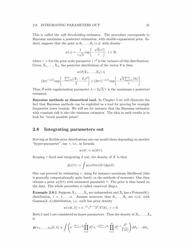
2.8. INTEGRATING PARAMETERS OUT 41
This is called the soft thresholding estimator. The procedure corresponds toBayesian maximum a posteriori estimation, with double-exponential prior. In-deed, suppose that the prior is θ1, . . . , θn i.i.d. with density
w(z) =1
τ√
2exp
[−√
2|z|τ
], z ∈ R,
where τ > 0 is the prior scale parameter ( τ2 is the variance of this distribution).Given X1, . . . , Xn, the posterior distribution of the vector θ is then
w(ϑ|X1, . . . , Xn) ∝
(2π)−n/2 exp
[−∑n
i=1(Xi − ϑi)2
2
]× (2πτ)−n/2 exp
[−√
2∑n
i=1 |ϑi|τ
].
Thus, θ with regularization parameter λ = 2√
2/τ is the maximum a posterioriestimator.
Bayesian methods as theoretical tool. In Chapter 5 we will illustrate thefact that Bayesian methods can be exploited as a tool for proving for examplefrequentist lower bounds. We will see for instance that the Bayesian estimatorwith constant risk is also the minimax estimator. The idea in such results is tolook for “worst possible priors”.
2.8 Integrating parameters out
Striving at flexible prior distributions one can model them depending on another“hyper-parameter”, say τ , i.e., in formula
w(ϑ) := w(ϑ|τ).
Keeping τ fixed and integrating ϑ out, the density of X is then
p(x|τ) :=
∫p(x|ϑ)w(ϑ|τ)dµ(ϑ).
One can proceed by estimating τ , using for instance maximum likelihood (thisis generally computationally quite hard), or the methods of moments. One thenobtains a prior w(ϑ|τ) with estimated parameter τ . The prior is thus based onthe data. The whole procedure is called empirical Bayes.
Example 2.8.1 SupposeX1, . . . , Xn are independent andXi has a Poisson(θi)-distribution, i = 1, . . . , n. Assume moreover that θ1, . . . , θn are i.i.d. withGamma(k, λ)-distribution, i.e., each has prior density
w(z|k, λ) = e−λzzk−1λk/Γ(k), z > 0.
Both k and λ are considered as hyper-parameters. Then the density ofX1, . . . , Xn
is
p(x1, . . . , xn|k, λ) ∝∫ (
e−∑ni=1 ϑi
n∏i=1
ϑxii e−λ∑ni=1 ϑi
n∏i=1
ϑk−1i
λk
Γ(k)
)dϑ1 · · · dϑn.
42 CHAPTER 2. DECISION THEORY
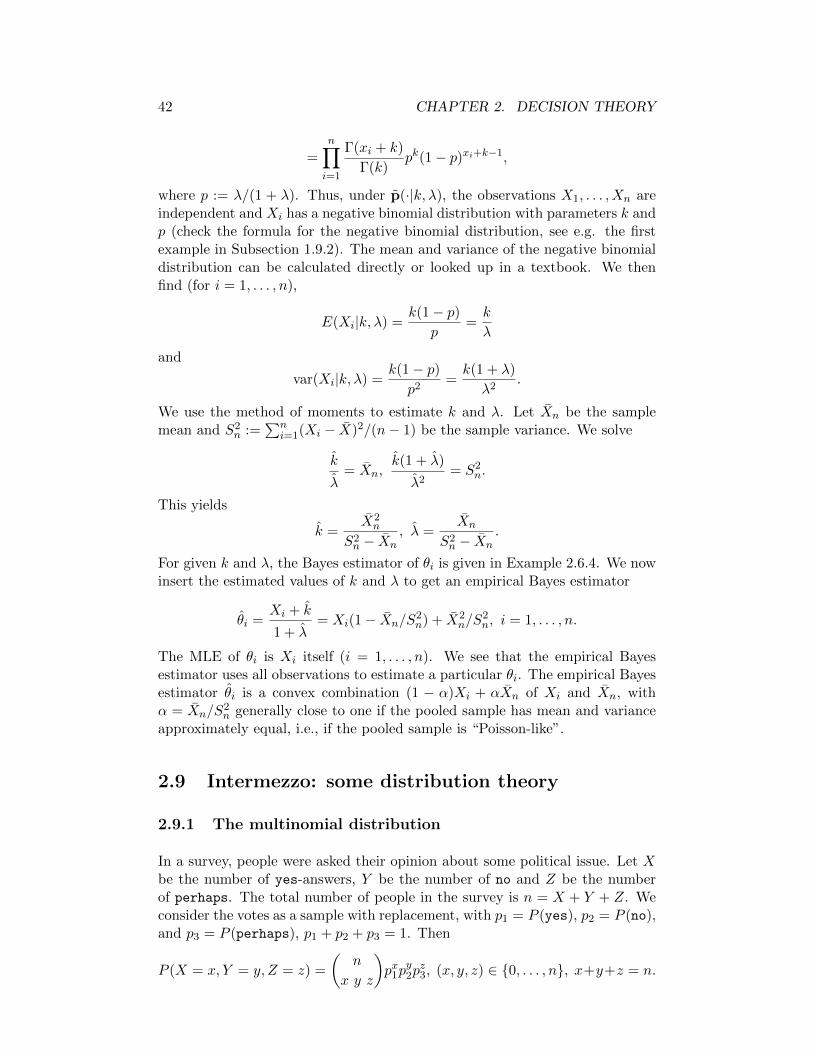
=
n∏i=1
Γ(xi + k)
Γ(k)pk(1− p)xi+k−1,
where p := λ/(1 + λ). Thus, under p(·|k, λ), the observations X1, . . . , Xn areindependent and Xi has a negative binomial distribution with parameters k andp (check the formula for the negative binomial distribution, see e.g. the firstexample in Subsection 1.9.2). The mean and variance of the negative binomialdistribution can be calculated directly or looked up in a textbook. We thenfind (for i = 1, . . . , n),
E(Xi|k, λ) =k(1− p)
p=k
λ
and
var(Xi|k, λ) =k(1− p)
p2=k(1 + λ)
λ2.
We use the method of moments to estimate k and λ. Let Xn be the samplemean and S2
n :=∑n
i=1(Xi − X)2/(n− 1) be the sample variance. We solve
k
λ= Xn,
k(1 + λ)
λ2= S2
n.
This yields
k =X2n
S2n − Xn
, λ =Xn
S2n − Xn
.
For given k and λ, the Bayes estimator of θi is given in Example 2.6.4. We nowinsert the estimated values of k and λ to get an empirical Bayes estimator
θi =Xi + k
1 + λ= Xi(1− Xn/S
2n) + X2
n/S2n, i = 1, . . . , n.
The MLE of θi is Xi itself (i = 1, . . . , n). We see that the empirical Bayesestimator uses all observations to estimate a particular θi. The empirical Bayesestimator θi is a convex combination (1 − α)Xi + αXn of Xi and Xn, withα = Xn/S
2n generally close to one if the pooled sample has mean and variance
approximately equal, i.e., if the pooled sample is “Poisson-like”.
2.9 Intermezzo: some distribution theory
2.9.1 The multinomial distribution
In a survey, people were asked their opinion about some political issue. Let Xbe the number of yes-answers, Y be the number of no and Z be the numberof perhaps. The total number of people in the survey is n = X + Y + Z. Weconsider the votes as a sample with replacement, with p1 = P (yes), p2 = P (no),and p3 = P (perhaps), p1 + p2 + p3 = 1. Then
P (X = x, Y = y, Z = z) =
(n
x y z
)px1p
y2pz3, (x, y, z) ∈ 0, . . . , n, x+y+z = n.
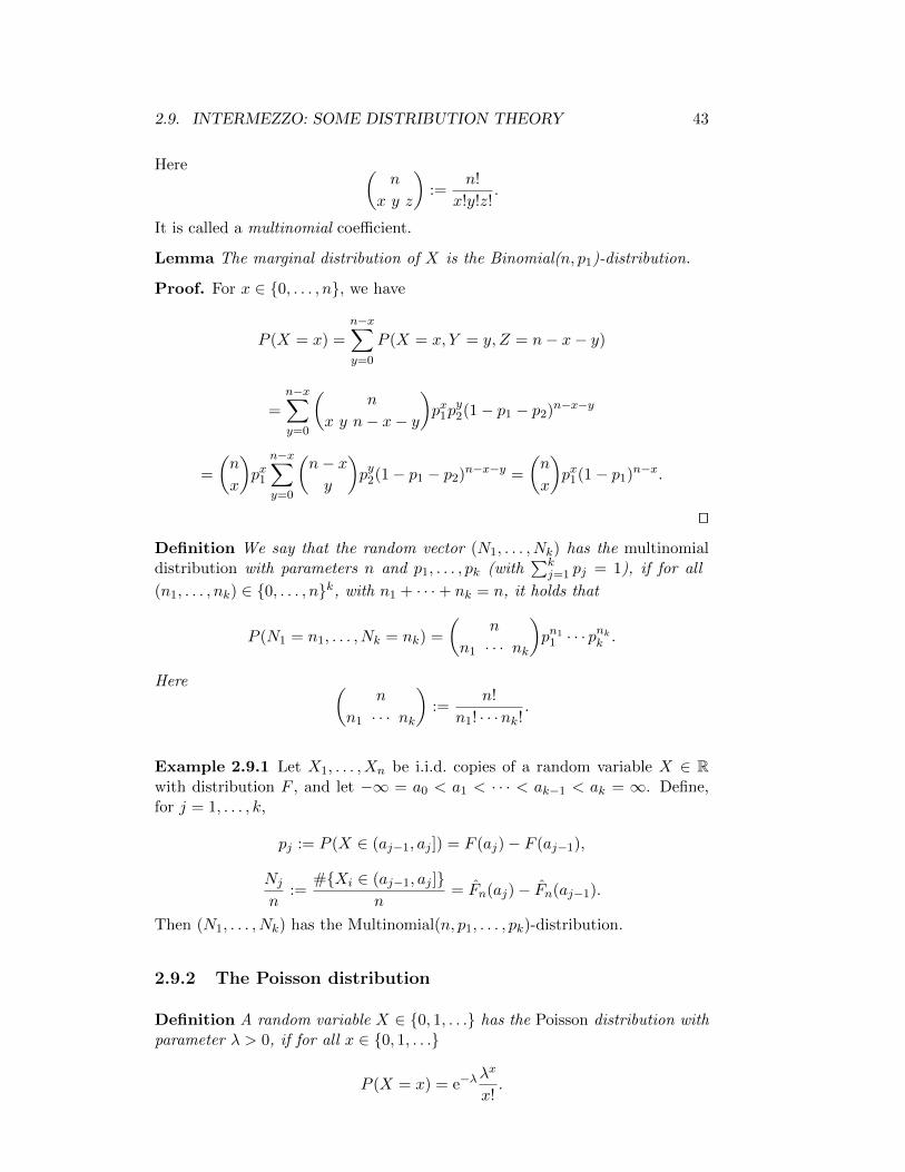
2.9. INTERMEZZO: SOME DISTRIBUTION THEORY 43
Here (n
x y z
):=
n!
x!y!z!.
It is called a multinomial coefficient.
Lemma The marginal distribution of X is the Binomial(n, p1)-distribution.
Proof. For x ∈ 0, . . . , n, we have
P (X = x) =n−x∑y=0
P (X = x, Y = y, Z = n− x− y)
=
n−x∑y=0
(n
x y n− x− y
)px1p
y2(1− p1 − p2)n−x−y
=
(n
x
)px1
n−x∑y=0
(n− xy
)py2(1− p1 − p2)n−x−y =
(n
x
)px1(1− p1)n−x.
tu
Definition We say that the random vector (N1, . . . , Nk) has the multinomialdistribution with parameters n and p1, . . . , pk (with
∑kj=1 pj = 1), if for all
(n1, . . . , nk) ∈ 0, . . . , nk, with n1 + · · ·+ nk = n, it holds that
P (N1 = n1, . . . , Nk = nk) =
(n
n1 · · · nk
)pn1
1 · · · pnkk .
Here (n
n1 · · · nk
):=
n!
n1! · · ·nk!.
Example 2.9.1 Let X1, . . . , Xn be i.i.d. copies of a random variable X ∈ Rwith distribution F , and let −∞ = a0 < a1 < · · · < ak−1 < ak = ∞. Define,for j = 1, . . . , k,
pj := P (X ∈ (aj−1, aj ]) = F (aj)− F (aj−1),
Nj
n:=
#Xi ∈ (aj−1, aj ]n
= Fn(aj)− Fn(aj−1).
Then (N1, . . . , Nk) has the Multinomial(n, p1, . . . , pk)-distribution.
2.9.2 The Poisson distribution
Definition A random variable X ∈ 0, 1, . . . has the Poisson distribution withparameter λ > 0, if for all x ∈ 0, 1, . . .
P (X = x) = e−λλx
x!.
44 CHAPTER 2. DECISION THEORY
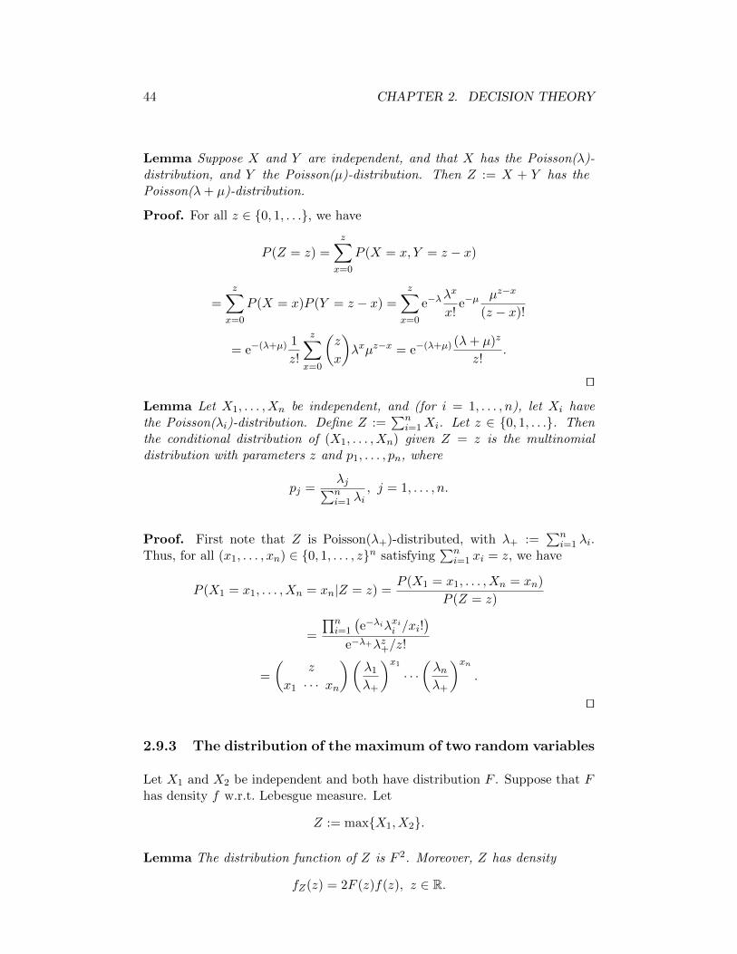
Lemma Suppose X and Y are independent, and that X has the Poisson(λ)-distribution, and Y the Poisson(µ)-distribution. Then Z := X + Y has thePoisson(λ+ µ)-distribution.
Proof. For all z ∈ 0, 1, . . ., we have
P (Z = z) =
z∑x=0
P (X = x, Y = z − x)
=
z∑x=0
P (X = x)P (Y = z − x) =
z∑x=0
e−λλx
x!e−µ
µz−x
(z − x)!
= e−(λ+µ) 1
z!
z∑x=0
(z
x
)λxµz−x = e−(λ+µ) (λ+ µ)z
z!.
tu
Lemma Let X1, . . . , Xn be independent, and (for i = 1, . . . , n), let Xi havethe Poisson(λi)-distribution. Define Z :=
∑ni=1Xi. Let z ∈ 0, 1, . . .. Then
the conditional distribution of (X1, . . . , Xn) given Z = z is the multinomialdistribution with parameters z and p1, . . . , pn, where
pj =λj∑ni=1 λi
, j = 1, . . . , n.
Proof. First note that Z is Poisson(λ+)-distributed, with λ+ :=∑n
i=1 λi.Thus, for all (x1, . . . , xn) ∈ 0, 1, . . . , zn satisfying
∑ni=1 xi = z, we have
P (X1 = x1, . . . , Xn = xn|Z = z) =P (X1 = x1, . . . , Xn = xn)
P (Z = z)
=
∏ni=1
(e−λiλxii /xi!
)e−λ+λz+/z!
=
(z
x1 · · · xn
)(λ1
λ+
)x1· · ·(λnλ+
)xn.
tu
2.9.3 The distribution of the maximum of two random variables
Let X1 and X2 be independent and both have distribution F . Suppose that Fhas density f w.r.t. Lebesgue measure. Let
Z := maxX1, X2.
Lemma The distribution function of Z is F 2. Moreover, Z has density
fZ(z) = 2F (z)f(z), z ∈ R.
2.10. SUFFICIENCY 45
Proof. We have for all z,
P (Z ≤ z) = P (maxX1, X2 ≤ z)
= P (X1 ≤ z,X2 ≤ z) = F 2(z).
If F has density f , then (Lebesgue)-almost everywhere,
f(z) =d
dzF (z).
So the derivative of F 2 exists almost everywhere, and
d
dzF 2(z) = 2F (z)f(z).
tu
Let X := (X1, X2). The conditional density of X given Z = z has density
fX(x1, x2|z) =
f(x2)2F (z) if x1 = z and x2 < zf(x1)2F (z) if x1 < z and x2 = z0 else
.
The conditional distribution function of X1 given Z = z is
FX1(x1|z) =
F (x1)2F (z) , x1 < z1, x1 ≥ z
.
Note thus that this distribution has a jump of size 1/2 at z.
2.10 Sufficiency
Let S : X → Y be some given map. We consider the statistic S = S(X).Throughout, by the phrase for all possible s, we mean for all s for which con-ditional distributions given S = s are defined (in other words: for all s in thesupport of the distribution of S, which may depend on θ).
Definition We call S sufficient for θ ∈ Θ if for all θ, and all possible s, theconditional distribution
Pθ(X ∈ ·|S(X) = s)
does not depend on θ.
Example 2.10.1 Let X1, . . . , Xn be i.i.d., and have the Bernoulli distributionwith probability θ ∈ (0, 1) of success: (for i = 1, . . . , n)
Pθ(Xi = 1) = 1− Pθ(Xi = 0) = θ.
Take S =∑n
i=1Xi. Then S is sufficient for θ: for all possible s,
IPθ(X1 = x1, . . . , Xn = xn|S = s) =1(ns
) , n∑i=1
xi = s.
46 CHAPTER 2. DECISION THEORY
Example 2.10.2 Let X := (X1, . . . , Xn), withX1, . . . , Xn i.i.d. and Poisson(θ)-distributed. Take S =
∑ni=1Xi. Then S has the Poisson(nθ)-distribution. For
all possible s, the conditional distribution of X given S = s is the multinomialdistribution with parameters s and (p1, . . . , pn) = ( 1
n , . . . ,1n):
IPθ(X1 = x1, . . . , Xn = xn|S = s) =
(s
x1 · · · xn
)(1
n
)s,
n∑i=1
xi = s.
This distribution does not depend on θ, so S is sufficient for θ.
Example 2.10.3 Let X1 and X2 be independent, and both have the exponen-tial distribution with parameter θ > 0. The density of e.g., X1 is then
fX1(x; θ) = θe−θx, x > 0.
Let S = X1 +X2. Verify that S has density
fS(s; θ) = sθ2e−θs, s > 0.
(This is the Gamma(2, θ)-distribution.) For all possible s, the conditional den-sity of (X1, X2) given S = s is thus
fX1,X2(x1, x2|S = s) =1
s, x1 + x2 = s.
Hence, S is sufficient for θ.
Example 2.10.4 Let X1, . . . , Xn be an i.i.d. sample from a continuous dis-tribution F . Then S := (X(1), . . . , X(n)) is sufficient for F : for all possibles = (s1, . . . , sn) (s1 < . . . < sn), and for (xq1 , . . . , xqn) = s,
IPθ
((X1, . . . , Xn) = (x1, . . . , xn)
∣∣∣∣(X(1), . . . , X(n)) = s
)=
1
n!.
Example 2.10.5 Let X1 and X2 be independent, and both uniformly dis-tributed on the interval [0, θ], with θ > 0. Define Z := X1 +X2.
Lemma The random variable Z has density
fZ(z; θ) =
z/θ2 if 0 ≤ z ≤ θ(2θ − z)/θ2 if θ ≤ z ≤ 2θ
.
Proof. First, assume θ = 1. Then the distribution function of Z is
FZ(z) =
z2/2 0 ≤ z ≤ 11− (2− z)2/2 1 ≤ z ≤ 2
.
So the density is then
fZ(z) =
z 0 ≤ z ≤ 12− z 1 ≤ z ≤ 2
.
2.10. SUFFICIENCY 47
For general θ, the result follows from the uniform case by the transformationZ 7→ θZ, which maps fZ into fZ(·/θ)/θ. tu
The conditional density of (X1, X2) given Z = z ∈ (0, 2θ) is now
fX,X2(x1, x2|Z = z; θ) =
1z 0 ≤ z ≤ θ
12θ−z θ ≤ z ≤ 2θ
.
This depends on θ, so Z is not sufficient for θ.
Consider now S := maxX1, X2. The conditional density of (X1, X2) givenS = s ∈ (0, θ) is
fX1,X2(x1, x2|S = s) =1
2s, 0 ≤ x1 < s, x2 = s or x1 = s, 0 ≤ x2 < s.
This does not depend on θ, so S is sufficient for θ.
Knowing the sufficient statistic S one can forget about the original data Xwithout loosing information. Indeed, the following lemma says that any deci-sion based on the original data X can be replaced by a randomized one whichdepends only on S and which has the same risk.
Lemma 2.10.1 Suppose S is sufficient for θ. Let d : X → A be some decision.Then there is a randomized decision δ(S) that only depends on S, such that
R(θ, δ(S)) = R(θ, d), ∀ θ.
Proof. Let X∗s be a random variable with distribution P (X ∈ ·|S = s). Then,by construction, for all possible s, the conditional distribution, given S = s,of X∗s and X are equal. It follows that X and X∗S have the same distribution.Formally, let us write Qθ for the distribution of S. Then
Pθ(X∗S ∈ ·) =
∫P (X∗s ∈ ·|S = s)dQθ(s)
=
∫P (X ∈ ·|S = s)dQθ(s) = Pθ(X ∈ ·).
The result of the lemma follows by taking δ(s) := d(X∗s ). tu.
2.10.1 Rao-Blackwell
The result of Rao-Blackwell says that in the case of convex loss a decisionbased on the original data X can be replaced by a decision based only on Swith smaller, or not worse, risk. Randomization is not needed here.
Lemma 2.10.2 (Rao Blackwell) Suppose that S is sufficient for θ. Supposemoreover that the action space A ⊂ Rp is convex, and that for each θ, themap a 7→ L(θ, a) is convex. Let d : X → A be a decision, and define d′(s) :=E(d(X)|S = s) (assumed to exist). Then
R(θ, d′) ≤ R(θ, d), ∀ θ.
48 CHAPTER 2. DECISION THEORY
Proof. Jensen’s inequality says that for a convex function g,
E(g(X)) ≥ g(EX).
Hence, ∀ θ,
E
(L
(θ, d(X)
)∣∣∣∣S = s
)≥ L
(θ,E
(d(X)|S = s
))= L(θ, d′(s)).
By the iterated expectations lemma, we arrive at
R(θ, d) = EθL(θ, d(X))
= EθE
(L
(θ, d(X)
)∣∣∣∣S) ≥ EθL(θ, d′(S)).
tu
2.10.2 Factorization Theorem of Neyman
Theorem 2.10.1 (Factorization Theorem of Neyman) Suppose Pθ : θ ∈ Θis dominated by a σ-finite measure ν. Let pθ := dPθ/dν denote the densities.Then S is sufficient for θ if and only if one can write pθ in the form
pθ(x) = gθ(S(x))h(x), ∀ x, θ
for some functions gθ(·) ≥ 0 and h(·) ≥ 0.
Proof in the discrete case. Suppose X takes only the values a1, a2, . . . ∀ θ(so we may take ν to be the counting measure). Let Qθ be the distribution ofS:
Qθ(s) :=∑
j: S(aj)=s
Pθ(X = aj).
The conditional distribution of X given S is
Pθ(X = x|S = s) =Pθ(X = x)
Qθ(s), S(x) = s.
(⇒) If S is sufficient for θ, the above does not depend on θ, but is only afunction of x, say h(x). So we may write for S(x) = s,
Pθ(X = x) = Pθ(X = x|S = s)Qθ(S = s) = h(x)gθ(s),
with gθ(s) = Qθ(S = s).
(⇐) Inserting pθ(x) = gθ(S(x))h(x), we find
Qθ(s) = gθ(s)∑
j: S(aj)=s
h(aj),
2.10. SUFFICIENCY 49
This gives in the formula for Pθ(X = x|S = s),
Pθ(X = x|S = s) =h(x)∑
j: S(aj)=sh(aj)
which does not depend on θ. tu
Remark The proof for the general case is along the same lines, but does havesome subtle elements!
Corollary 2.10.1 The likelihood is LX(θ) = pθ(X) = gθ(S)h(X). Hence, themaximum likelihood estimator θ = arg maxθ LX(θ) = arg maxθ gθ(S) dependsonly on the sufficient statistic S.
Corollary 2.10.2 The Bayes decision is
dBayes(X) = arg mina∈A
l(X, a),
where
l(x, a) = E(L(θ, a)|X = x) =
∫L(ϑ, a)w(ϑ|x)dµ(ϑ)
=
∫L(ϑ, a)gϑ(S(x))w(ϑ)dµ(ϑ)h(x)/p(x).
So
dBayes(X) = arg mina∈A
∫L(ϑ, a)gϑ(S)w(ϑ)dµ(ϑ),
which only depends on the sufficient statistic S.
Example 2.10.6 Let X1, . . . , Xn be i.i.d., and uniformly distributed on theinterval [0, θ]. Then the density of X = (X1, . . . , Xn) is
pθ(x1, . . . , xn) =1
θnl0 ≤ minx1, . . . , xn ≤ maxx1, . . . , xn ≤ θ
= gθ(S(x1, . . . , xn))h(x1, . . . , xn),
with
gθ(s) :=1
θnls ≤ θ,
and
h(x1, . . . , xn) := l0 ≤ minx1, . . . , xn.
Thus, S = maxX1, . . . , Xn is sufficient for θ.
50 CHAPTER 2. DECISION THEORY
2.10.3 Exponential families
Definition A k-dimensional exponential family is a family of distributions Pθ :θ ∈ Θ, dominated by some σ-finite measure ν, with densities pθ = dPθ/dν ofthe form
pθ(x) = exp
[ k∑j=1
cj(θ)Tj(x)− d(θ)
]h(x).
Note In case of a k-dimensional exponential family, the k-dimensional statisticS(X) = (T1(X), . . . , Tk(X)) is sufficient for θ.
Note If X1, . . . , Xn is an i.i.d. sample from a k-dimensional exponential family,then the distribution of X = (X1, . . . , Xn) is also in a k-dimensional exponentialfamily. The density of X is then (for x := (x1, . . . , xn)),
pθ(x) =n∏i=1
pθ(xi) = exp[k∑j=1
ncj(θ)Tj(x)− nd(θ)]n∏i=1
h(xi),
where, for j = 1, . . . , k,
Tj(x) =1
n
n∑i=1
Tj(xi).
Hence S(X) = (T1(X), . . . , Tk(X)) is then sufficient for θ.
Note The functions Tj and cj are not uniquely defined.
Example 2.10.7 If X is Poisson(θ)-distributed, we have
pθ(x) = e−θθx
x!
= exp[x log θ − θ] 1
x!.
Hence, we may take T (x) = x, c(θ) = log θ, and d(θ) = θ.
Example 2.10.8 If X has the Binomial(n, θ)-distribution, we have
pθ(x) =
(n
x
)θx(1− θ)n−x
=
(n
x
)(θ
1− θ
)x(1− θ)n
=
(n
x
)exp
[x log(
θ
1− θ) + n log(1− θ)
].
So we can take T (x) = x, c(θ) = log(θ/(1− θ)), and d(θ) = −n log(1− θ).
2.10. SUFFICIENCY 51
Example 2.10.9 If X has the Negative Binomial(k, θ)-distribution we have
pθ(x) =Γ(x+ k)
Γ(k)x!θk(1− θ)x
=Γ(x+ k)
Γ(k)x!exp[x log(1− θ) + k log(θ)].
So we may take T (x) = x, c(θ) = log(1− θ) and d(θ) = −k log(θ).
Example 2.10.10 Let X have the Gamma(k, θ)-distribution (with k known).Then
pθ(x) = e−θxxk−1 θk
Γ(k)
=xk−1
Γ(k)exp[−θx+ k log θ].
So we can take T (x) = x, c(θ) = −θ, and d(θ) = −k log θ.
Example 2.10.11 Let X have the Gamma(k, λ)-distribution, and let θ =(k, λ). Then
pθ(x) = e−λxxk−1 λk
Γ(k)
= exp[−λx+ (k − 1) log x+ k log λ− log Γ(k)].
So we can take T1(x) = x, T2(x) = log x, c(θ) = −λ, c2(θ) = (k − 1), andd(θ) = −k log λ+ log Γ(k).
Example 2.10.12 Let X be N (µ, σ2)-distributed, and let θ = (µ, σ). Then
pθ(x) =1√2πσ
exp
[−(x− µ)2
2σ2
]
=1√2π
exp
[xµ
σ2− x2
2σ2− µ2
2σ2− log σ
].
So we can take T1(x) = x, T2(x) = x2, c1(θ) = µ/σ2, c2(θ) = −1/(2σ2), andd(θ) = µ2/(2σ2) + log(σ).
2.10.4 Canonical form of an exponential family
In this subsection, we assume regularity conditions, such as existence of deriva-tives, and inverses, and permission to interchange differentiation and integra-tion.
Let Θ ⊂ Rk, and let Pθ : θ ∈ Θ be a family of probability measures dominatedby a σ-finite measure ν. Define the densities
pθ :=dPθdν
.
52 CHAPTER 2. DECISION THEORY
Definition We call Pθ : θ ∈ Θ an exponential family in canonical form, if
pθ(x) = exp
[ k∑j=1
θjTj(x)− d(θ)
]h(x).
Note that d(θ) is the normalizing constant
d(θ) = log
∫ exp
[ k∑j=1
θjTj(x)
]h(x)dν(x)
.
We let
d(θ) :=∂
∂θd(θ) =
∂∂θ1
d(θ)...
∂∂θk
d(θ)
denote the vector of first derivatives, and
d(θ) :=∂2
∂θ∂θ>d(θ) =
(∂2d(θ)
∂θj∂θj′
)denote the k × k matrix of second derivatives. Further, we write
T (X) :=
T1(X)...
Tk(X)
, EθT (X) :=
EθT1(X)...
EθTk(X)
,
and we write the k × k covariance matrix of T (X) as
Covθ(T (X)) :=
(covθ(Tj(X), Tj′(X))
).
Lemma We have (under regularity)
EθT (X) = d(θ), Covθ(T (X)) = d(θ).
Proof. By the definition of d(θ), we find
d(θ) =∂
∂θlog
(∫exp
[θ>T (x)
]h(x)dν(x)
)
=
∫exp
[θ>T (x)
]T (x)h(x)dν(x)
∫exp
[θ>T (x)
]h(x)dν(x)
=
∫exp
[θ>T (x)− d(θ)
]T (x)h(x)dν(x)
2.10. SUFFICIENCY 53
=
∫pθ(x)T (x)dν(x) = EθT (X),
and
d(θ) =
∫exp
[θ>T (x)
]T (x)T (x)>h(x)dν(x)
∫exp
[θ>T (x)
]h(x)dν(x)
−
(∫exp
[θ>T (x)
]T (x)h(x)dν(x)
)(∫exp
[θ>T (x)
]T (x)h(x)dν(x)
)>(∫
exp
[θ>T (x)
]h(x)dν(x)
)2
=
∫exp
[θ>T (x)− d(θ)
]T (x)T (x)>h(x)dν(x)
−(∫
exp
[θ>T (x)− d(θ)
]T (x)h(x)dν(x)
)
×(∫
exp
[θ>T (x)− d(θ)
]T (x)h(x)dν(x)
)>=
∫pθ(x)T (x)T (x)>dν(x)
−(∫
pθ(x)T (x)dν(x)
)(∫pθ(x)T (x)dν(x)
)>= EθT (X)T (X)> −
(EθT (X)
)(EθT (X)
)>= Covθ(T (X)).
tu
Let us now simplify to the one-dimensional case, that is Θ ⊂ R. Consider anexponential family, not necessarily in canonical form:
pθ(x) = exp[c(θ)T (x)− d(θ)]h(x).
We can put this in canonical form by reparametrizing
θ 7→ c(θ) := γ (say),
to get
pγ(x) = exp[γT (x)− d0(γ)]h(x),
where
d0(γ) = d(c−1(γ)).
It follows that
EθT (X) = d0(γ) =d(c−1(γ))
c(c−1(γ))=d(θ)
c(θ), (2.2)
54 CHAPTER 2. DECISION THEORY
and
varθ(T (X)) = d0(γ) =d(c−1(γ))
[c(c−1(γ))]2− d(c−1(γ))c(c−1(γ))
[c(c−1(γ))]3
=d(θ)
[c(θ)]2− d(θ)c(θ)
[c(θ)]3=
1
[c(θ)]2
(d(θ)− d(θ)
c(θ)c(θ)
). (2.3)
For an arbitrary (but regular) family of densities pθ : θ ∈ Θ, with (again forsimplicity) Θ ⊂ R, we define the score function
sθ(x) :=d
dθlog pθ(x),
and the Fisher information for estimating θ
I(θ) := varθ(sθ(X))
(see also Chapter 3 and 6).
Lemma We have (under regularity)
Eθsθ(X) = 0,
and
I(θ) = −Eθsθ(X),
where sθ(x) := ddθsθ(x).
Proof. The results follow from the fact that densities integrate to one, assumingthat we may interchange derivatives and integrals:
Eθsθ(X) =
∫sθ(x)pθ(x)dν(x)
=
∫d log pθ(x)
dθpθ(x)dν(x) =
∫dpθ(x)/dθ
pθ(x)pθ(x)dν(x)
=
∫d
dθpθ(x)dν(x) =
d
dθ
∫pθ(x)dν(x) =
d
dθ1 = 0,
and
Eθsθ(X) = Eθ
[d2pθ(X)/dθ2
pθ(X)−(dpθ(X)/dθ
pθ(X)
)2]= Eθ
[d2pθ(X)/dθ2
pθ(X)
]− Eθs2
θ(X).
Now, Eθs2θ(X) equals varθsθ(X), since Eθsθ(X) = 0. Moreover,
Eθ
[d2pθ(X)/dθ2
pθ(X)
]=
∫d2
dθ2pθ(x)dν(x) =
d2
dθ2
∫pθ(x)dν(x) =
d2
dθ21 = 0.
tu
2.10. SUFFICIENCY 55
In the special case that Pθ : θ ∈ Θ is a one-dimensional exponential family,the densities are of the form
pθ(x) = exp[c(θ)T (x)− d(θ)]h(x).
Hencesθ(x) = c(θ)T (x)− d(θ).
The equality Eθsθ(X) = 0 implies that
EθT (X) =d(θ)
c(θ),
which re-establishes (2.2). One moreover has
sθ(x) = c(θ)T (x)− d(θ).
Hence, the inequality varθ(sθ(X)) = −Eθsθ(X) implies
[c(θ)]2varθ(T (X)) = −c(θ)EθT (X) + d(θ)
= d(θ)− d(θ)
c(θ)c(θ),
which re-establishes (2.3). In addition, it follows that
I(θ) = d(θ)− d(θ)
c(θ)c(θ).
The Fisher information for estimating γ = c(θ) is
I0(γ) = d0(γ) =I(θ)
[c(θ)]2.
More generally, the Fisher information for estimating a differentiable functiong(θ) of the parameter θ, is equal to I(θ)/[g(θ)]2.
Example
LetX ∈ 0, 1 have the Bernoulli-distribution with success parameter θ ∈ (0, 1):
pθ(x) = θx(1− θ)1−x = exp
[x log
(θ
1− θ
)+ log(1− θ)
], x ∈ 0, 1.
We reparametrize:
γ := c(θ) = log
(θ
1− θ
),
which is called the log-odds ratio. Inverting gives
θ =eγ
1 + eγ,
and hence
d(θ) = − log(1− θ) = log
(1 + eγ
):= d0(γ).
56 CHAPTER 2. DECISION THEORY
Thus
d0(γ) =eγ
1 + eγ= θ = EθX,
and
d0(γ) =eγ
1 + eγ− e2γ
(1 + eγ)2=
eγ
(1 + eγ)2= θ(1− θ) = varθ(X).
The score function is
sθ(x) =d
dθ
[x log
(θ
1− θ
)+ log(1− θ)
]
=x
θ(1− θ)− 1
1− θ.
The Fisher information for estimating the success parameter θ is
Eθs2θ(X) =
varθ(X)
[θ(1− θ)]2=
1
θ(1− θ),
whereas the Fisher information for estimating the log-odds ratio γ is
I0(γ) = θ(1− θ).
2.10.5 Minimal sufficiency
Definition We say that two likelihoods Lx(θ) and Lx′(θ) are proportional at(x, x′), if
Lx(θ) = Lx′(θ)c(x, x′),∀ θ,
for some constant c(x, x′).A statistic S is called minimal sufficient if S(x) = S(x′) for all x and x′ forwhich the likelihoods are proportional.
Example 2.10.13 LetX1 . . . , Xn be independent andN (θ, 1)-distributed. ThenS =
∑ni=1Xi is sufficient for θ. We moreover have
logLx(θ) = S(x)θ − nθ2
2−∑n
i=1 x2i
2− log(2π)/2.
So
logLx(θ)− logLx′(θ) = (S(x)− S(x′))θ −∑n
i=1 x2i −
∑ni=1(x′i)
2
2,
which equals,
log c(x,x′), ∀ θ,
for some function c, if and only if S(x) = S(x′). So S is minimal sufficient.
2.10. SUFFICIENCY 57
Example 2.10.14 LetX1, . . . , Xn be independent and Laplace-distributed withlocation parameter θ. Then
logLx(θ) = −(log 2)/2−√
2n∑i=1
|xi − θ|,
so
logLx(θ)− logLx′(θ) = −√
2n∑i=1
(|xi − θ| − |x′i − θ|)
which equalslog c(x,x′), ∀ θ,
for some function c, if and only if (x(1), . . . , x(n)) = (x′(1), . . . , x′(n)). So the order
statistics X(1), . . . , X(n) are minimal sufficient.

58 CHAPTER 2. DECISION THEORY
Chapter 3
Unbiased estimators
3.1 What is an unbiased estimator?
Let X ∈ X denote the observations. The distribution P of X is assumed tobe a member of a given class Pθ : θ ∈ Θ of distributions. The parameter ofinterest in this chapter is γ := g(θ), with g : Θ→ R (for simplicity, we initiallyassume γ to be one-dimensional).
Let T : X → R be an estimator of g(θ).
Definition The bias of T = T (X) is
biasθ(T ) := EθT − g(θ).
The estimator T is called unbiased if
biasθ(T ) = 0, ∀ θ.
Thus, unbiasedness means that there is no systematic error: EθT = g(θ). Werequire this for all θ.
Example 3.1.1 Let X ∼ Binomial(n, θ), 0 < θ < 1. We have
EθT (X) =
n∑k=0
(n
k
)θk(1− θ)n−kT (k) := q(θ).
Note that q(θ) is a polynomial in θ of degree at most n. So only parametersg(θ) which are polynomials of degree at most n can be estimated unbiasedly. Itmeans that there exists no unbiased estimator of, for example,
√θ or θ/(1− θ).
Example 3.1.2 Let X ∼ Poisson(θ). Then
EθT (X) =
∞∑k=0
e−θθk
k!T (k) := e−θp(θ).
59
60 CHAPTER 3. UNBIASED ESTIMATORS
Note that p(θ) is a power series in θ. Thus only parameters g(θ) which are apower series in θ times e−θ can be estimated unbiasedly. An example is theprobability of early failure
g(θ) := e−θ = Pθ(X = 0).
An unbiased estimator of e−θ is for instance
T (X) = lX = 0.
As another example, suppose the parameter of interest is
g(θ) := e−2θ.
An unbiased estimator is
T (X) =
+1 if X is even−1 if X is odd
.
This estimator does not make sense at all!
Example 3.1.3 Let X1, . . . , Xn be i.i.d. N (µ, σ2), and let θ = (µ, σ2) ∈ R ×R+. Then
S2 :=1
n− 1
n∑i=1
(Xi − X)2
is an unbiased estimator of σ2. But S is not an unbiased estimator of σ. Infact, one can show that there does not exist any unbiased estimator of σ!
We conclude that requiring unbiasedness can have disadvantages: unbiased es-timators do not always exist, and if they do, they can be nonsensical. Moreover,the property of unbiasedness is not preserved under taking nonlinear transfor-mations.
3.2 UMVU estimators
Lemma 3.2.1 We have the following equality for the mean square error:
Eθ|T − g(θ)|2 = bias2θ(T ) + varθ(T ).
In other words, the mean square error consists of two components, the (squared)bias and the variance. This is called the bias-variance decomposition. As wewill see, it is often the case that an attempt to decrease the bias results in anincrease of the variance (and vise versa).
Example 3.2.1 Let X1, . . . , Xn be i.i.d. N (µ, σ2)-distributed. Both µ and σ2
are unknown parameters: θ := (µ, σ2).
3.2. UMVU ESTIMATORS 61
Case i Suppose the mean µ is our parameter of interest. Consider the estimatorT := λX, where 0 ≤ λ ≤ 1. Then the bias is decreasing in λ, but the varianceis increasing in λ:
Eθ|T − µ|2 = (1− λ)2µ2 + λ2σ2/n.
The right hand side can be minimized as a function of λ. The minimum isattained at
λopt :=µ2
σ2/n+ µ2.
However, λoptX is not an estimator as it depends on the unknown parameters.
Case ii Suppose σ2 is the parameter of interest. Let S2 be the sample variance:
S2 :=1
n− 1
n∑i=1
(Xi − X)2.
It is known that S2 is unbiased. But does it also have small mean square error?Let us compare it with the estimator
σ2 :=1
n
n∑i=1
(Xi − X)2.
To compute the mean square errors of these two estimators, we first recall that∑ni=1(Xi − X)2
σ2∼ χ2
n−1,
a χ2-distribution with n−1 degrees of freedom. The χ2-distribution is a specialcase of the Gamma-distribution, namely
χ2n−1 = Γ
(n− 1
2,1
2
).
Thus 1
Eθ
(n∑i=1
(Xi − X)2/σ2
)= n− 1, var
(n∑i=1
(Xi − X)2/σ2
)= 2(n− 1).
It follows that
Eθ|S2 − σ2|2 = var(S2) =σ4
(n− 1)22(n− 1) =
2σ4
n− 1,
and
Eθσ2 =
n− 1
nσ2,
biasθ(σ2) = − 1
nσ2,
1If Y has a Γ(k, λ)-distribution, then EY = k/λ and var(Y ) = k/λ2.
62 CHAPTER 3. UNBIASED ESTIMATORS
so that
Eθ|σ2 − σ2|2 = bias2θ(σ
2) + varθ(σ2) =
σ4
n2+σ4
n22(n− 1) =
σ4(2n− 1)
n2.
Conclusion: the mean square error of σ2 is smaller than the mean square errorof S2!
Generally, it is not possible to construct an estimator that possesses the bestamong all of all desirable properties. We therefore fix one property: unbi-asedness (despite its disadvantages), and look for good estimators among theunbiased ones.
Definition An unbiased estimator T ∗is called UMVU (Uniform MinimumVariance Unbiased) if for any other unbiased estimator T ,
varθ(T∗) ≤ varθ(T ), ∀ θ.
Suppose that T is unbiased, and that S is sufficient. Let
T ∗ := E(T |S).
The distribution of T given S does not depend on θ, so T ∗ is also an estimator.Moreover, it is unbiased:
EθT∗ = Eθ(E(T |S)) = EθT = g(θ).
By conditioning on S, “superfluous” variance in the sample is killed. Indeed,the following lemma (which is a general property of conditional distributions)shows that T ∗ cannot have larger variance than T :
varθ(T∗) ≤ varθ(T ), ∀ θ.
Lemma 3.2.2 Let Y and Z be two random variables. Then
var(Y ) = var(E(Y |Z)) + Evar(Y |Z).
Proof. It holds that
var(E(Y |Z)) = E
[E(Y |Z)
]2
−[E(E(Y |Z))
]2
= E[E(Y |Z)]2 − [EY ]2,
and
Evar(Y |Z) = E
[E(Y 2|Z)− [E(Y |Z)]2
]= EY 2 − E[E(Y |Z)]2.
Hence, when adding up, the term E[E(Y |Z)]2 cancels out, and what is left overis exactly the variance
var(Y ) = EY 2 − [EY ]2.
tu
3.2. UMVU ESTIMATORS 63
3.2.1 Complete statistics
The question arises: can we construct an unbiased estimator with even smallervariance than T ∗ = E(T |S)? Note that T ∗ depends on X only via S = S(X),i.e., it depends only on the sufficient statistic. In our search for UMVU estima-tors, we may restrict our attention to estimators depending only on S. Thus, ifthere is only one unbiased estimator depending only on S, it has to be UMVU.
Definition A statistic S is called complete if we have the following implication:
Eθh(S) = 0 ∀ θ ⇒ h(S) = 0, Pθ − a.s.,∀ θ.
Here, h is a function of S not depending on θ.
Lemma 3.2.3 (Lehmann-Scheffe) Let T be an unbiased estimator of g(θ),with, for all θ, finite variance. Moreover, let S be sufficient and complete.Then T ∗ := E(T |S) is UMVU.
Proof. We already noted that T ∗ = T ∗(S) is unbiased and that varθ(T∗) ≤
varθ(T ) ∀ θ. If T ′(S) is another unbiased estimator of g(θ), we have
Eθ(T (S)− T ′(S)) = 0,∀ θ.
Because S is complete, this implies
T ∗ = T ′, Pθ − a.s.
tu
To check whether a statistic is complete, one often needs somewhat sophisti-cated tools from analysis/integration theory. In the next two examples, we onlysketch the proofs of completeness.
Example 3.2.2 Let X1, . . . , Xn be i.i.d. Poisson(θ)-distributed. We want toestimate g(θ) := e−θ, the probability of early failure. An unbiased estimator is
T (X1, . . . , Xn) := lX1 = 0.
A sufficient statistic is
S :=
n∑i=1
Xi.
We now check whether S is complete. Its distribution is the Poisson(nθ)-distribution. We therefore have for any function h,
Eθh(S) =∞∑k=0
e−nθ(nθ)k
k!h(k).
The equation
Eθh(S) = 0 ∀ θ,
64 CHAPTER 3. UNBIASED ESTIMATORS
thus implies∞∑k=0
(nθ)k
k!h(k) = 0 ∀ θ.
Let f be a function with Taylor expansion at zero. Then
f(x) =
∞∑k=0
xk
k!f (k)(0).
The left hand side can only be zero for all x if f ≡ 0, in which case alsof (k)(0) = 0 for all k. Thus (h(k) takes the role of f (k)(0) and nθ the role of x),we conclude that h(k) = 0 for all k, i.e., that S is complete.
So we know from the Lehmann-Scheffe Lemma that T ∗ := E(T |S) is UMVU.Now,
P (T = 1|S = s) = P (X1 = 0|S = s)
=e−θe−(n−1)θ[(n− 1)θ]s/s!
e−nθ(nθ)s/s!=
(n− 1
n
)s.
Hence
T ∗ =
(n− 1
n
)Sis UMVU.
Example 3.2.3 Let X1, . . . , Xn be i.i.d. Uniform[0, θ]-distributed, and g(θ) :=θ. We know that S := maxX1, . . . , Xn is sufficient. The distribution functionof S is
FS(s) = Pθ(maxX1, . . . , Xn ≤ s) =(sθ
)n, 0 ≤ s ≤ θ.
Its density is thus
fS(s) =nsn−1
θn, 0 ≤ s ≤ θ.
Hence, for any (measurable) function h,
Eθh(S) =
∫ θ
0h(s)
nsn−1
θnds.
If
Eθh(S) = 0 ∀ θ,
it must hold that ∫ θ
0h(s)sn−1ds = 0 ∀ θ.
Differentiating w.r.t. θ gives
h(θ)θn−1 = 0 ∀ θ,
3.2. UMVU ESTIMATORS 65
which implies h ≡ 0. So S is complete.
It remains to find a statistic T ∗ that depends only on S and that is unbiased.We have
EθS =
∫ θ
0snsn−1
θnds =
n
n+ 1θ.
So S itself is not unbiased, it is too small. But this can be easily repaired: take
T ∗ =n+ 1
nS.
Then, by the Lehmann-Scheffe Lemma, T ∗ is UMVU.
In the case of an exponential family, completeness holds for a sufficient statisticif the parameter space is “of the same dimension” as the sufficient statistic.This is stated more formally in the following lemma. We omit the proof.
Lemma 3.2.4 Let for θ ∈ Θ,
pθ(x) = exp
[ k∑j=1
cj(θ)Tj(x)− d(θ)
]h(x).
Consider the set
C := (c1(θ), . . . , ck(θ)) : θ ∈ Θ ⊂ Rk.
Suppose that C is truly k-dimensional (that is, not of dimension smaller thank), i.e., it contains an open ball in Rk. (Or an open cube
∏kj=1(aj , bj).) Then
S := (T1, . . . , Tk) is complete.
Example 3.2.4 Let X1, . . . , Xn be i.i.d. with Γ(k, λ)-distribution. Both k andλ are assumed to be unknown, so that θ := (k, λ). We moreover let Θ := R2
+.The density f of the Γ(k, λ)-distribution is
f(z) =λk
Γ(k)e−λzzk−1, z > 0.
Hence,
pθ(x) = exp
[−λ
n∑i=1
xi + (k − 1)n∑i=1
log xi − d(θ)
]h(x),
whered(k, λ) = −nk log λ+ n log Γ(k),
andh(x) = lxi > 0, i = 1, . . . , n.
It follows that ( n∑i=1
Xi,
n∑i=1
logXi
)is sufficient and complete.
66 CHAPTER 3. UNBIASED ESTIMATORS
Example 3.2.5 Consider two independent samples from normal distributions:X1, . . . Xn i.i.d. N (µ, σ2)-distributed and Y1, . . . , Ym be i.i.d. N (ν, τ2)-distributed.
Case i If θ = (µ, ν, σ2, τ2) ∈ R2 × R2+, one can easily check that
S :=
( n∑i=1
Xi,n∑i=1
X2i ,
m∑j=1
Yj ,m∑j=1
Y 2j
)
is sufficient and complete.
Case ii If µ, σ2 and τ2 are unknown, and ν = µ, then S of course remainssufficient. One can however show that S is not complete. Difficult question:does a sufficient and complete statistic exist?
3.3 The Cramer-Rao lower bound
Let Pθ : θ ∈ Θ be a collection of distributions on X , dominated by a σ-finitemeasure ν. We denote the densities by
pθ :=dPθdν
, θ ∈ Θ.
In this section, we assume that Θ is a one-dimensional open interval (the ex-tension to a higher-dimensional parameter space will be handled in the nextsection).
We will impose the following two conditions:
Condition I The set
A := x : pθ(x) > 0
does not depend on θ.
Condition II (Differentiability in L2) For all θ and for a function sθ : X → Rsatisfying
I(θ) := Eθsθ(X)2 <∞,
it holds that
limh→0
Eθ
(pθ+h(X)− pθ(X)
hpθ(X)− sθ(X)
)2
= 0.
Definition If I and II hold, we call sθ the score function, and I(θ) the Fisherinformation.
Lemma 3.3.1 Assume conditions I and II. Then
Eθsθ(X) = 0,∀ θ.
3.3. THE CRAMER-RAO LOWER BOUND 67
Proof. Under Pθ, we only need to consider values x with pθ(x) > 0, that is,we may freely divide by pθ, without worrying about dividing by zero.
Observe that
Eθ
(pθ+h(X)− pθ(X)
pθ(X)
)=
∫A
(pθ+h − pθ)dν = 0,
since densities integrate to 1, and both pθ+h and pθ vanish outside A. Thus,
|Eθsθ(X)|2 =
∣∣∣∣Eθ(pθ+h(X)− pθ(X)
hpθ(X)− sθ(X)
)∣∣∣∣2
≤ Eθ(pθ+h(X)− pθ(X)
hpθ(X)− sθ(X)
)2
→ 0.
tu
Note Thus I(θ) = varθ(sθ(X)).
Remark If pθ(x) is differentiable for all x, we can take (under regularity con-ditions)
sθ(x) :=d
dθlog pθ(x) =
pθ(x)
pθ(x),
where
pθ(x) :=d
dθpθ(x).
Remark Suppose X1, . . . , Xn are i.i.d. with density pθ, and sθ = pθ/pθ exists.The joint density is
pθ(x) =n∏i=1
pθ(xi),
so that (under conditions I and II) the score function for n observations is
sθ(x) =
n∑i=1
sθ(xi).
The Fisher information for n observations is thus
I(θ) = varθ(sθ(X)) =
n∑i=1
varθ(sθ(Xi)) = nI(θ).
Theorem 3.3.1 (The Cramer-Rao lower bound) Suppose conditions I and IIare met, and that T is an unbiased estimator of g(θ) with finite variance. Theng(θ) has a derivative, g(θ) := dg(θ)/dθ, equal to
g(θ) = cov(T, sθ(X)).
Moreover,
varθ(T ) ≥ [g(θ)]2
I(θ), ∀ θ.
68 CHAPTER 3. UNBIASED ESTIMATORS
Proof. We first show differentiability of g. As T is unbiased, we have
g(θ + h)− g(θ)
h=Eθ+hT (X)− EθT (X)
h
=1
h
∫T (pθ+h − pθ)dν = EθT (X)
pθ+h(X)− pθ(X)
hpθ(X)
= EθT (X)
(pθ+h(X)− pθ(X)
hpθ(X)− sθ(X)
)+ EθT (X)sθ(X)
= Eθ
(T (X)− gθ
)(pθ+h(X)− pθ(X)
hpθ(X)− sθ(X)
)+ EθT (X)sθ(X)
→ EθT (X)sθ(X),
as, by the Cauchy-Schwarz inequality∣∣∣∣Eθ(T (X)− gθ)(
pθ+h(X)− pθ(X)
hpθ(X)− sθ(X)
)∣∣∣∣2≤ varθ(T )Eθ
(pθ+h(X)− pθ(X)
hpθ(X)− sθ(X)
)2
→ 0.
Thus,g(θ) = EθT (X)sθ(X) = covθ(T, sθ(X)).
The last inequality holds because Eθsθ(X) = 0. By Cauchy-Schwarz,
[g(θ)]2 = |covθ(T, sθ(X))|2
≤ varθ(T )varθ(sθ(X)) = varθ(T )I(θ).
tu
Definition We call [g(θ)]2/I(θ), θ ∈ Θ, the Cramer Rao lower bound (CRLB)(for estimating g(θ)).
Example 3.3.1 Let X1, . . . , Xn be i.i.d. Exponential(θ), θ > 0. The densityof a single observation is then
pθ(x) = θe−θx, x > 0.
Let g(θ) := 1/θ, and T := X. Then T is unbiased, and varθ(T ) = 1/(nθ2). Wenow compute the CRLB. With g(θ) = 1/θ, one has g(θ) = −1/θ2. Moreover,
log pθ(x) = log θ − θx,
sosθ(x) = 1/θ − x,
and hence
I(θ) = varθ(X) =1
θ2.
The CRLB for n observations is thus
[g(θ)]2
nI(θ)=
1
nθ2.
In other words, T reaches the CRLB.
3.3. THE CRAMER-RAO LOWER BOUND 69
Example 3.3.2 Suppose X1, . . . , Xn are i.i.d. Poisson(θ), θ > 0. Then
log pθ(x) = −θ + x log θ − log x!,
sosθ(x) = −1 +
x
θ,
and hence
I(θ) = varθ
(X
θ
)=
varθ(X)
θ2=
1
θ.
One easily checks that X reaches the CRLB for estimating θ.
Let now g(θ) := e−θ. The UMVU estimator of g(θ) is
T :=
(1− 1
n
)∑ni=1Xi
.
To compute its variance, we first compute
EθT2 =
∞∑k=0
(1− 1
n
)2k (nθ)k
k!e−nθ
= e−nθ∞∑k=0
1
k!
((n− 1)2θ
n
)k= e−nθ exp
[(n− 1)2θ
n
]= exp
[(1− 2n)θ
n
].
Thus,varθ(T ) = EθT
2 − [EθT ]2 = EθT2 − e−2θ
= e−2θ
(eθ/n − 1
)> θe−2θ/n≈ θe−2θ/n for n large
.
As g(θ) = −e−θ, the CRLB is
[g(θ)]2
nI(θ)=θe−2θ
n.
We conclude that T does not reach the CRLB, but the gap is small for n large.
For the next result, we:
Recall Let X and Y be two real-valued random variables. The correlationbetween X and Y is
ρ(X,Y ) :=cov(X,Y )√
var(X)var(Y ).
We have
|ρ(X,Y )| = 1⇔ ∃ constants a, b : Y = aX + b (a.s.).
The next lemma shows that the CRLB can only be reached within exponentialfamilies, thus is only tight in a rather limited context.
70 CHAPTER 3. UNBIASED ESTIMATORS
Lemma 3.3.2 Assume conditions I and II, with sθ = pθ/pθ. Suppose T isunbiased for g(θ), and that T reaches the Cramer-Rao lower bound. Then Pθ :θ ∈ Θ forms a one-dimensional exponential family: there exist functions c(θ),d(θ), and h(x) such that for all θ,
pθ(x) = exp[c(θ)T (X)− d(θ)]h(x), x ∈ X .
Moreover, c(θ) and d(θ) are differentiable, say with derivatives c(θ) and d(θ)respectively. We furthermore have the equality
g(θ) = d(θ)/c(θ), ∀ θ.
Proof. By Theorem 3.3, when T reaches the CRLB, we must have
varθ(T ) =|cov(T, sθ(X))|2
varθ(sθ(X)),
i.e., then the correlation between T and sθ(X) is ±1. Thus, there exist constantsa(θ) and b(θ) (depending on θ), such that
sθ(X) = a(θ)T (X)− b(θ). (3.1)
But, as sθ = pθ/pθ = d log pθ/dθ, we can take primitives:
log pθ(x) = c(θ)T (x)− d(θ) + h(x),
where c(θ) = a(θ), d(θ) = b(θ) and h(x) is constant in θ. Hence,
pθ(x) = exp[c(θ)T (x)− d(θ)]h(x),
with h(x) = exp[h(x)].
Moreover, the equation (3.1) tells us that
Eθsθ(X) = a(θ)EθT − b(θ) = a(θ)g(θ)− b(θ).
Because Eθsθ(X) = 0, this implies that g(θ) = b(θ)/a(θ). tu
3.4 Higher-dimensional extensions
Expectations and covariances of random vectors
Let X ∈ Rp be a p-dimensional random vector. Then EX is a p-dimensionalvector, and
Σ := Cov(X) := EXXT − (EX)(EX)T
3.4. HIGHER-DIMENSIONAL EXTENSIONS 71
is a p × p matrix containing all variances (on the diagonal) and covariances(off-diagonal). Note that Σ is positive semi-definite: for any vector a ∈ Rp, wehave
var(aTX) = aTΣa ≥ 0.
Some matrix algebra
Let V be a symmetric matrix. If V is positive (semi-)definite, we write thisas V > 0 (V ≥ 0). One then has that V = W 2, where W is also positive(semi-)definite.
Auxiliary lemma. Suppose V > 0. Then
maxa∈Rp
|aT c|2
aTV a= cTV −1c.
Proof. Write V = W 2, and b := Wa, d := W−1c. Then aTV a = bT b = ‖b‖2and aT c = bTd. By Cauchy-Schwarz
maxb∈Rp
|bTd|2
‖b‖2= ‖d‖2 = dTd = cTV −1c.
tu
We will now present the CRLB in higher dimensions. To simplify the exposition,we will not carefully formulate the regularity conditions, that is, we assumederivatives to exist and that we can interchange differentiation and integrationat suitable places.
Consider a parameter space Θ ⊂ Rp. Let
g : Θ→ R,
be a given function. Denote the vector of partial derivatives as
g(θ) :=
∂g(θ)/∂θ1...
∂g(θ)/∂θp
.
The score vector is defined as
sθ(·) :=
∂ log pθ/∂θ1...
∂ log pθ/∂θp
.
The Fisher information matrix is
I(θ) = Eθsθ(X)sTθ (X) = Covθ(sθ(X)).
72 CHAPTER 3. UNBIASED ESTIMATORS
Theorem 3.4.1 Let T be an unbiased estimator of g(θ). Then, under regular-ity conditions,
varθ(T ) ≥ g(θ)T I(θ)−1g(θ).
Proof. As in the one-dimensional case, one can show that, for j = 1, . . . , p,
gj(θ) = covθ(T, sθ,j(X)).
Hence, for all a ∈ Rp,
|aT g(θ)|2 = |covθ(T, aT sθ(X))|2
≤ varθ(T )varθ(aT sθ(X))
= varθ(T )aT I(θ)a.
Combining this with the auxiliary lemma gives
varθ(T ) ≥ maxa∈Rp
|aT g(θ)|2
aT I(θ)a= g(θ)T I(θ)−1g(θ).
tu
Corollary 3.4.1 As a consequence, one obtains a lower bound for unbiasedestimators of higher-dimensional parameters of interest. As example, let g(θ) :=θ = (θ1, . . . , θp)
T , and suppose that T ∈ Rp is an unbiased estimator of θ. Then,for all a ∈ Rp, aTT is an unbiased estimator of aT θ. Since aT θ has derivativea, the CRLB gives
varθ(aTT ) ≥ aT I(θ)−1a.
But
varθ(aTT ) = aTCovθ(T )a.
So for all a,
aTCovθ(T )a ≥ aT I(θ)−1a,
in other words, Covθ(T ) ≥ I(θ)−1, that is, Covθ(T ) − I(θ)−1 is positive semi-definite.
3.5 Uniformly most powerful tests
3.5.1 An example
Let X1, . . . , Xn be i.i.d. copies of a Bernoulli random variable X ∈ 0, 1 withsuccess parameter θ ∈ (0, 1):
Pθ(X = 1) = 1− Pθ(X = 0) = θ.
3.5. UNIFORMLY MOST POWERFUL TESTS 73
We consider three testing problems. The chosen level in all three problems isα = 0.05.
Problem 1
We want to test, at level α, the hypothesis
H0 : θ = 1/2 := θ0,
against the alternative
H1 : θ = 1/4 := θ1.
Let T :=∑n
i=1Xi be the number of successes (T is a sufficient statistic), andconsider the randomized test
φ(T ) :=
1 if T < t0q if T = t00 if T > t0
,
where q ∈ (0, 1), and where t0 is the critical value of the test. The constants qand t0 ∈ 0, . . . , n are chosen in such a way that the probability of rejectingH0 when it is in fact true, is equal to α:
Pθ0(H0 rejected) = Pθ0(T ≤ t0 − 1) + qPθ0(T = t0) := α.
Thus, we take t0 in such a way that
Pθ0(T ≤ t0 − 1) ≤ α, Pθ0(T ≤ t0) > α,
(i.e., t0 − 1 = q+(α) with q+ the quantile function defined in Section 1.6) and
q =α− Pθ0(T ≤ t0 − 1)
Pθ0(T = t0).
Because φ = φNP is the Neyman Pearson test, it is the most powerful test (atlevel α) (see the Neyman Pearson Lemma in Section 2.2). The power of thetest is β(θ1), where
β(θ) := Eθφ(T ).
Numerical Example
Let n = 7. Then
Pθ0(T = 0) =
(1/2
)7
= 0.0078,
Pθ0(T = 1) =(
71
)(1/2
)7
= 0.0546,
Pθ0(T ≤ 1) = 0.0624 > α,
so we choose t0 = 1. Moreover
q =0.05− 0.0078
0.0546=
422
546.
74 CHAPTER 3. UNBIASED ESTIMATORS
The power is now
β(θ1) = Pθ1(T = 0) + qPθ1(T = 1)
=
(3/4
)7
+422
546
(7
1
)(3/4
)6(1/4
)= 0.1335 +
422
5460.3114.
Problem 2
Consider now testing
H0 : θ0 = 1/2,
against
H1 : θ < 1/2.
In Problem 1, the construction of the test φ is independent of the value θ1 < θ0.So φ is most powerful for all θ1 < θ0. We say that φ is uniformly most powerful(German: gleichmassig machtigst) for the alternative H1 : θ < θ0.
Problem 3
We now want to test
H0 : θ ≥ 1/2,
against the alternative
H1 : θ < 1/2.
Recall the function
β(θ) := Eθφ(T ).
The level of φ is defined as
supθ≥1/2
β(θ).
We have
β(θ) = Pθ(T ≤ t0 − 1) + qPθ(T = t0)
= (1− q)Pθ(T ≤ t0 − 1) + qPθ(T ≤ t0).
Observe that if θ1 < θ0, small values of T are more likely under Pθ1 than underPθ0 :
Pθ1(T ≤ t) > Pθ0(T ≤ t), ∀ t ∈ 0, 1, . . . , n.
Thus, β(θ) is a decreasing function of θ. It follows that the level of φ is
supθ≥1/2
β(θ) = β(1/2) = α.
Hence, φ is uniformly most powerful for H0 : θ ≥ 1/2 against H1 : θ < 1/2.
3.5. UNIFORMLY MOST POWERFUL TESTS 75
3.5.2 UMP tests and exponential families
Let P := Pθ : θ ∈ Θ be a family of probability measures. Let Θ0 ⊂ Θ,Θ1 ⊂ Θ, and Θ0 ∩Θ1 = ∅. Based on observations X, with distribution P ∈ P,we consider the general testing problem, at level α, for
H0 : θ ∈ Θ0,
against
H1 : θ ∈ Θ1.
We say that a test φ has level α if
supθ∈Θ0
Eθφ(X) ≤ α.
Definition A test φ is called Uniformly Most Powerful (UMP) if• φ has level α,• for all tests φ′ with level α, it holds that Eθφ
′(X) ≤ Eθφ(X) ∀ θ ∈ Θ1.
We now simplify the situation to the case where Θ is an interval in R, and tothe testing problem
H0 : θ ≤ θ0,
against
H1 : θ > θ0.
We also suppose that P is dominated by a σ-finite measure ν.
Theorem 3.5.1 Suppose that P is a one-dimensional exponential family
dPθdν
(x) := pθ(x) = exp[c(θ)T (x)− d(θ)]h(x).
Assume moreover that c(θ) is a strictly increasing function of θ. Then a UMPtest φ is
φ(T (x)) :=
1 if T (x) > t0q if T (x) = t00 if T (x) < t0
,
where q and t0 are chosen in such a way that Eθ0φ(T ) = α.
Proof. The Neyman Pearson test for H0 : θ = θ0 against H1 : θ = θ1 is
φNP(x) =
1 if pθ1(x)/pθ0(x) > c0
q0 if pθ1(x)/pθ0(x) = c0
0 if pθ1(x)/pθ0(x) < c0
,
where q0 and c0 are chosen in such a way that Eθ0φNP(X) = α. We have
pθ1(x)
pθ0(x)= exp
[(c(θ1)− c(θ0))T (X)− (d(θ1)− d(θ0))
].
76 CHAPTER 3. UNBIASED ESTIMATORS
Hence
pθ1(x)
pθ0(x)
>=<c ⇔ T (x)
>=<t ,
where t is some constant (depending on c, θ0 and θ1). Therefore, φ = φNP. Itfollows that φ is most powerful for H0 : θ = θ0 against H1 : θ = θ1. Because φdoes not depend on θ1, it is therefore UMP for H0 : θ = θ0 against H1 : θ > θ0.
We will now prove that β(θ) := Eθφ(T ) is increasing in θ. Let
pθ(t) = exp[c(θ)t− d(θ)]
be the density of T with respect to dominating measure ν. For ϑ > θ
pϑ(t)
pθ(t)= exp
[(c(ϑ)− c(θ))t− (d(ϑ)− d(θ))
],
which is increasing in t. Moreover, we have∫pϑdν =
∫pθdν = 1.
Therefore, there must be a point s0 where the two densities cross:pϑ(t)pθ(t) ≤ 1 for t ≤ s0
pϑ(t)pθ(t) ≥ 1 for t ≥ s0
.
But then
β(ϑ)− β(θ) =
∫φ(t)[pϑ(t)− pθ(t)]dν(t)
=
∫t≤s0
φ(t)[pϑ(t)− pθ(t)]dν(t) +
∫t≥s0
φ(t)[pϑ(t)− pθ(t)]dν(t)
≥ φ(s0)
∫[pϑ(t)− pθ(t)]dν(t) = 0.
So indeed β(θ) is increasing in θ.
But then
supθ≤θ0
β(θ) = β(θ0) = α.
Hence, φ has level α. Because any other test φ′ with level α must haveEθ0φ
′(X) ≤ α, we conclude that φ is UMP.
tu
Example 3.5.1 LetX1, . . . , Xn be an i.i.d. sample from theN (µ0, σ2)-distribution,
with µ0 known, and σ2 > 0 unknown. We want to test
H0 : σ2 ≤ σ20,
against
3.5. UNIFORMLY MOST POWERFUL TESTS 77
H1 : σ2 > σ20.
The density of the sample is
pσ2(x1, . . . , xn) = exp
[− 1
2σ2
n∑i=1
(xi − µ0)2 − n
2log(2πσ2)
].
Thus, we may take
c(σ2) = − 1
2σ2,
and
T (X) =n∑i=1
(Xi − µ0)2.
The function c(σ2) is strictly increasing in σ2. So we let φ be the test whichrejects H0 for large values of T (X).
Example 3.5.2 LetX1, . . . , Xn be an i.i.d. sample from the Bernoulli(θ)-distribution,0 < θ < 1. Then
pθ(x1, . . . , xn) = exp
[log
(θ
1− θ
) n∑i=1
xi + n log(1− θ)].
We can take
c(θ) = log
(θ
1− θ
),
which is strictly increasing in θ. Then T (X) =∑n
i=1Xi.
Right-sided alternative
H0 : θ ≤ θ0 ,
against
H1 : θ > θ0 .
The UMP test is
φR(T ) :=
1 T > tRqR T = tR0 T < tR
.
The function βR(θ) := EθφR(T ) is strictly increasing in θ.
Left-sided alternative
H0 : θ ≥ θ0 ,
against
H1 : θ < θ0 .
The UMP test is
φL(T ) :=
1 T < tLqL T = tL0 T > tL
.
78 CHAPTER 3. UNBIASED ESTIMATORS
The function βL(θ) := EθφL(T ) is strictly decreasing in θ.
Two-sided alternative
H0 : θ = θ0 ,
against
H1 : θ 6= θ0 .
The test φR is most powerful for θ > θ0, whereas φL is most powerful for θ < θ0.Hence, a UMP test does not exist for the two-sided alternative.
3.5.3 Unbiased tests
Consider again the general case: P := Pθ : θ ∈ Θ is a family of probabilitymeasures, the spaces Θ0, and Θ1 are disjoint subspaces of Θ, and the testingproblem is
H0 : θ ∈ Θ0,
against
H1 : θ ∈ Θ1.
The significance level is α (α < 1).
As we have seen in Example 3.5.2, uniformly most powerful tests do not alwaysexist. We therefore restrict attention to a smaller class of tests, and look foruniformly most powerful tests in the smaller class.
DefinitionA test φ is called unbiased (German unverfalscht) if for all θ ∈ Θ0
and all ϑ ∈ Θ1,Eθφ(X) ≤ Eϑφ(X).
Definition A test φ is called Uniformly Most Powerful Unbiased (UMPU) if• φ has level α,• φ is unbiased,• for all unbiased tests φ′ with level α, one has Eθφ
′(X) ≤ Eθφ(X) ∀ θ ∈ Θ1.
We return to the special case where Θ ⊂ R is an interval. We consider testing
H0 : θ = θ0,
against
H1 : θ 6= θ0.
The following theorem presents the UMPU test. We omit the proof (see e.g.Lehmann ...).
Theorem 3.5.2 Suppose P is a one-dimensional exponential family:
dPθdν
(x) := pθ(x) = exp[c(θ)T (x)− d(θ)]h(x),
3.5. UNIFORMLY MOST POWERFUL TESTS 79
with c(θ) strictly increasing in θ. Then a UMPU test is
φ(T (x)) :=
1 if T (x) < tL or T (x) > tRqL if T (x) = tLqR if T (x) = tR0 if tL < T (x) < tR
,
where the constants tR , tL, qR and qL are chosen in such a way that
Eθ0φ(X) = α,d
dθEθφ(X)
∣∣∣∣θ=θ0
= 0.
Note Let φR a right-sided test as defined Theorem 3.5.1 with level at mostα and φL be the similarly defined left-sided test. Then βR(θ) = EθφR(T ) isstrictly increasing, and βL(θ) = EθφL(T ) is strictly decreasing. The two-sidedtest φ of Theorem 3.5.2 is a superposition of two one-sided tests. Writing
β(θ) = Eθφ(T ),
the one-sided tests are constructed in such a way that
β(θ) = βR(θ) + βL(θ).
Moreover, β(θ) should be minimal at θ = θ0, whence the requirement that itsderivative at θ0 should vanish. Let us see what this derivative looks like. Withthe notation used in the proof of Theorem 3.5.1, for a test φ depending only onthe sufficient statistic T ,
Eθφ(T ) =
∫φ(t) exp[c(θ)t− d(θ)]dν(t).
Hence, assuming we can take the differentiation inside the integral,
d
dθEθφ(T ) =
∫φ(t) exp[c(θ)t− d(θ)](c(θ)t− d(θ))dν(t)
= c(θ)covθ(φ(T ), T ).
Example 3.5.3 LetX1, . . . , Xn be an i.i.d. sample from theN (µ, σ20)-distribution,
with µ ∈ R unknown, and with σ20 known. We consider testing
H0 : µ = µ0,
against
H1 : µ 6= µ0.
A sufficient statistic is T :=∑n
i=1Xi. We have, for tL < tR,
Eµφ(T ) = IPµ(T > tR) + IPµ(T < tL)
= IPµ
(T − nµ√nσ0
>tR − nµ√
nσ0
)+ IPµ
(T − nµ√nσ0
<tL − nµ√nσ0
)
80 CHAPTER 3. UNBIASED ESTIMATORS
= 1− Φ
(tR − nµ√
nσ0
)+ Φ
(tL − nµ√nσ0
),
where Φ is the standard normal distribution function. To avoid confusion withthe test φ, we denote the standard normal density in this example by Φ. Thus,
d
dµEµφ(T ) =
n√nσ0
Φ
(tR − nµ√
nσ0
)− n√
nσ0Φ
(tL − nµ√nσ0
),
So puttingd
dµEµφ(T )
∣∣∣∣µ=µ0
= 0,
gives
Φ
(tR − nµ0√
nσ0
)= Φ
(tL − nµ0√
nσ0
),
or(tR − nµ0)2 = (tL − nµ0)2.
We take the solution (tL − nµ0) = −(tR − nµ0), (because the solution(tL − nµ0) = (tR − nµ0) leads to a test that always rejects, and hence doesnot have level α, as α < 1). Plugging this solution back in gives
Eµ0φ(T ) = 1− Φ
(tR − nµ0√
nσ0
)+ Φ
(− tR − nµ0√
nσ0
)= 2
(1− Φ
(tR − nµ0√
nσ0
)).
The requirement Eµ0φ(T ) = α gives us
Φ
(tR − nµ0√
nσ0
)= 1− α/2,
and hence
tR − nµ0 =√nσ0Φ−1(1− α/2), tL − nµ0 = −
√nσ0Φ−1(1− α/2).
3.5.4 Conditional tests
We now study the case where Θ is an interval in R2. We let θ = (β, γ), and weassume that γ is the parameter of interest. We aim at testing
H0 : γ ≤ γ0,
against the alternative
H1 : γ > γ0.
We assume moreover that we are dealing with an exponential family in canonicalform:
pθ(x) = exp[βT1(x) + γT2(x)− d(θ)]h(x).
Then we can restrict ourselves to tests φ(T ) depending only on the sufficientstatistic T = (T1, T2).
3.5. UNIFORMLY MOST POWERFUL TESTS 81
Lemma 3.5.1 Suppose that β : (β, γ0) ∈ Θ contains an open interval. Let
φ(T1, T2) =
1 if T2 > t0(T1)q(T1) if T2 = t0(T1)0 if T2 < t0(T1)
,
where the constants t0(T1) and q(T1) are allowed to depend on T1, and arechosen in such a way that
Eγ0
(φ(T1, T2)
∣∣∣∣T1
)= α.
Then φ is UMPU.
Sketch of proof.
Let pθ(t1, t2) be the density of (T1, T2) with respect to dominating measure ν:
pθ(t1, t2) := exp[βt1 + γt2 − d(θ)]h(t1, t2).
We assume ν(tt, t2) = ν1(t1)ν2(t2) is a product measure. The conditional den-sity of T2 given T1 = t1 is then
pθ(t2|t1) =exp[βt1 + γt2 − d(θ)]h(t1, t2)∫
s2exp[βt1 + γs2 − d(θ)]h(t1, s2)dν2(s2)
= exp[γt2 − d(γ|t1)]h(t1, t2),
where
d(γ|t1) := log
(∫s2
exp[γs2]h(t1, s2)dν2(s2)
).
In other words, the conditional distribution of T2 given T1 = t1- does not depend on β,- is a one-parameter exponential family in canonical form.This implies that given T1 = t1, φ is UMPU.
Result 1 The test φ has level α, i.e.
supγ≤γ0
E(β.γ)φ(T ) = E(β,γ0)φ(T ) = α, ∀ β.
Proof of Result 1.
supγ≤γ0
E(β,γ)φ(T ) ≥ E(β,γ0)φ(T ) = E(β,γ0)Eγ0(φ(T )|T1) = α.
Conversely,supγ≤γ0
E(β,γ)φ(T ) = supγ≤γ0
E(β,γ)Eγ(φ(T )|T1)︸ ︷︷ ︸≤α
≤ α.
Result 2 The test φ is unbiased.
82 CHAPTER 3. UNBIASED ESTIMATORS
Proof of Result 2. If γ > γ0, it holds that Eγ(φ(T )|T1) ≥ α, as the conditionaltest is unbiased. Thus, also, for all β,
E(β,γ)φ(T ) = E(β,γ)Eγ(φ(T )|T1) ≥ α,
i.e., φ is unbiased.
Result 3 Let φ′ be a test with level
α′ := supβ
supγ≤γ0
E(β,γ)φ′(T ) ≤ α,
and suppose moreover that φ′ is unbiased, i.e., that
supγ≤γ0
supβE(β,γ)φ
′(T ) ≤ infγ>γ0
infβE(β,γ)φ
′(T ).
Then, conditionally on T1, φ′ has level α′.
Proof of Result 3. As
α′ = supβ
supγ≤γ0
E(β,γ)φ′(T )
we know thatE(β,γ0)φ
′(T ) ≤ α′, ∀ β.
Conversely, the unbiasedness implies that for all γ > γ0,
E(β,γ)φ′(T ) ≥ α′,∀ β.
A continuity argument therefore gives
E(β,γ0)φ′(T ) = α′, ∀ β.
In other words, we have
E(β,γ0)(φ′(T )− α′) = 0,∀ β.
But then also
E(β,γ0)Eγ0
((φ′(T )− α′)
∣∣∣∣T1
)= 0, ∀ β,
which we can write asE(β,γ0)h(T1) = 0,∀ β.
The assumption that β : (β, γ0) ∈ Θ contains an open interval implies thatT1 is complete for (β, γ0). So we must have
h(T1) = 0, P(β,γ0)−a.s., ∀ β,
or, by the definition of h,
Eγ0(φ′(T )|T1) = α′, P(β,γ0) − a.s., ∀ β.
So conditionally on T1, the test φ′ has level α′.
3.5. UNIFORMLY MOST POWERFUL TESTS 83
Result 4 Let φ′ be a test as given in Result 3. Then φ′ can not be more powerfulthan φ at any (β, γ), with γ > γ0.
Proof of Result 4. By the Neyman Pearson lemma, conditionally on T1, wehave
Eγ(φ′(T )|T1) ≤ Eγ(φ(T )|T1), ∀ γ > γ0.
Thus also
E(β,γ)φ′(T ) ≤ E(β,γ)φ(T ), ∀ β, γ > γ0.
tu
Example 3.5.4 Consider two independent samples X = (X1, . . . , Xn) andY = (Y1, . . . , Ym), where X1, . . . , Xn are i.i.d. Poisson(λ)-distributed, andY1, . . . , Ym are i.i.d. Poisson(µ)-distributed. We aim at testing
H0 : λ ≤ µ,
against the alternative
H1 : λ > µ.
Define
β := log(µ), γ := log(λ/µ).
The testing problem is equivalent to
H0 : γ ≤ γ0,
against the alternative
H1 : γ > γ0,
where γ0 := 0.
The density is
pθ(x1, . . . , xn, y1, . . . , ym)
= exp
[log(λ)
n∑i=1
xi + log(µ)
m∑j=1
yj − nλ−mµ] n∏i=1
1
xi!
m∏j=1
1
yj !
= exp
[log(µ)(
n∑i=1
xi +m∑j=1
yj) + log(λ/µ)n∑i=1
xi − nλ−mµ]h(x,y)
= exp[βT1(x,y) + γT2(x)− d(θ)]h(x,y),
where
T1(X,Y) :=
n∑i=1
Xi +
m∑j=1
Yj ,
and
T2(X) :=
n∑i=1
Xi,
84 CHAPTER 3. UNBIASED ESTIMATORS
and
h(x,y) :=
n∏i=1
1
xi!
m∏j=1
1
yj !.
The conditional distribution of T2 given T1 = t1 is the Binomial(t1, p)-distribution,with
p =nλ
nλ+mµ=
eγ
1 + eγ.
Thus, conditionally on T1 = t1, using the observation T2 from the Binomial(t1, p)-distribution, we test
H0 : p ≤ p0,
against the alternative
H1 : p > p0,
where p0 := n/(n+m). This test is UMPU for the unconditional problem.

Chapter 4
Equivariant statistics
As we have seen in the previous chapter, it can be useful to restrict attentionto a collection of statistics satisfying certain desirable properties. In Chapter3, we restricted ourselves to unbiased estimators. In this chapter, equivariancewill be the key concept.
The data consists of i.i.d. real-valued random variables X1, . . . , Xn. We writeX := (X1, . . . , Xn). The density w.r.t. some dominating measure ν, of asingle observation is denoted by pθ. The density of X is pθ(x) =
∏i pθ(xi),
x = (x1, . . . , xn).
Location modelThen θ ∈ R is a location parameter, and we assume
Xi = θ + εi, i = 1, . . . , n.
We are interested in estimating θ. Both the parameter space Θ, as well as theaction space A, are the real line R.
Location-scale modelHere θ = (µ, σ), with µ ∈ R a location parameter and σ > 0 a scale parameter.We assume
Xi = µ+ σεi, i = 1, . . . , n.
The parameter space Θ and action space A are both R× (0,∞).
4.1 Equivariance in the location model
Definition A statistic T = T (X) is called location equivariant if for all con-stants c ∈ R and all x = (x1, . . . , xn),
T (x1 + c, . . . , xn + c) = T (x1, . . . , xn) + c.
85
86 CHAPTER 4. EQUIVARIANT STATISTICS
Examples
T =
XX(n+1
2) (n odd)
· · ·.
Definition A loss function L(θ, a) is called location invariant if for all c ∈ R,
L(θ + c, a+ c) = L(θ, a), (θ, a) ∈ R2.
In this section we abbreviate location equivariance (invariance) to simply equiv-ariance (invariance), and we assume throughout that the loss L(θ, a) is invari-ant.
Corollary If T is equivariant (and L(θ, a) is invariant), then
R(θ, T ) = EθL(θ, T (X)) = EθL(0, T (X)− θ)
= EθL(0, T (X− θ)) = EθL0[T (ε)],
where L0[a] := L(0, a) and ε := (ε1, . . . , εn). Because the distribution of ε doesnot depend on θ, we conclude that the risk does not depend on θ. We maytherefore omit the subscript θ in the last expression:
R(θ, T ) = EL0[T (ε)].
Since for θ = 0, we have the equality X = ε we may alternatively write
R(θ, T ) = E0L0[T (X)] = R(0, T ).
Definition An equivariant statistic T is called uniform minimum risk equivari-ant (UMRE) if
R(θ, T ) = mind equivariant
R(θ, d), ∀ θ,
or equivalently,
R(0, T ) = mind equivariant
R(0, d).
Lemma 4.1.1 Let Yi := Xi − Xn, i = 1, . . . , n, and Y := (Y1, . . . , Yn). Wehave
T equivariant ⇔ T (X) = T (Y) +Xn.
Proof.(⇒) Trivial.(⇐) Replacing X by X + c leaves Y unchanged (i.e. Y is invariant). SoT (X + c) = T (Y) +Xn + c = T (X) + c. tu
4.1. EQUIVARIANCE IN THE LOCATION MODEL 87
Theorem 4.1.1 Let Yi := Xi−Xn, i = 1, . . . , n, Y := (Y1, . . . , Yn), and define
T ∗(Y) := arg minvE
(L0[v + εn]
∣∣∣∣Y).Moreover, let
T ∗(X) := T ∗(Y) +Xn.
Then T ∗ is UMRE.
Proof. First, note that the distribution of Y does not depend on θ, so that T ∗
is indeed a statistic. It is also equivariant, by the previous lemma.
Let T be an equivariant statistic. Then T (X) = T (Y) +Xn. So
T (X)− θ = T (Y) + εn.
Hence
R(0, T ) = EL0[T (Y) + εn] = E
[E
(L0[T (Y) + εn]
∣∣∣∣Y)].But
E
(L0[T (Y) + εn]
∣∣∣∣Y) ≥ minvE
(L0[v + εn]
∣∣∣∣Y) = E
(L0[T ∗(Y) + εn]
∣∣∣∣Y).Hence,
R(0, T ) ≥ E[E
(L0[T ∗(Y) + εn]
∣∣∣∣Y)] = R(0, T ∗).
tu
Corollary 4.1.1 If we take quadratic loss
L(θ, a) := (a− θ)2,
we get L0[a] = a2, and so, for Y = X−Xn,
T ∗(Y) = arg minvE
((v + εn)2
∣∣∣∣Y)= −E(εn|Y),
and hence
T ∗(X) = Xn − E(εn|Y).
This estimator is called the Pitman estimator.
To investigate the case of quadratic risk further, we:
Note If (X,Z) has density f(x, z) w.r.t. Lebesgue measure, then the densityof Y := X − Z is
fY (y) =
∫f(y + z, z)dz.
88 CHAPTER 4. EQUIVARIANT STATISTICS
Lemma 4.1.2 Consider quadratic loss. Let p0 be the density of ε = (ε1, . . . , εn)w.r.t. Lebesgue measure. Then a UMRE statistic is
T ∗(X) =
∫zp0(X1 − z, . . . ,Xn − z)dz∫p0(X1 − z, . . . ,Xn − z)dz
.
Proof. Let Y = X−Xn. The random vector Y has density
fY(y1, . . . , yn−1, 0) =
∫p0(y1 + z, . . . , yn−1 + z, z)dz.
So the density of εn given Y = y = (y1, . . . , yn−1, 0) is
fεn(u) =p0(y1 + u, . . . , yn−1 + u, u)∫p0(y1 + z, . . . , yn−1 + z, z)dz
.
It follows that
E(εn|y) =
∫up0(y1 + u, . . . , yn−1 + u, u)du∫p0(y1 + z, . . . , yn−1 + z, z)dz
.
Thus
E(εn|Y) =
∫up0(Y1 + u, . . . , Yn−1 + u, u)du∫p0(Y1 + z, . . . , Yn−1 + z, z)dz
=
∫up0(X1 −Xn + u, . . . ,Xn−1 −Xn + u, u)du∫p0(X1 −Xn + z, . . . ,Xn−1 −Xn + z, z)dz
= Xn −∫zp0(X1 − z, . . . ,Xn−1 − z,Xn − z)dz∫p0(X1 + z, . . . ,Xn−1 + z,Xn + z)dz
.
Finally, recall that T ∗(X) = Xn − E(εn|Y). tu
Example 4.1.1 Suppose X1, . . . , Xn are i.i.d. Uniform[θ−1/2, θ+1/2], θ ∈ R.Then
p0(x) = l|x| ≤ 1/2.
We have
max1≤i≤n
|xi − z| ≤ 1/2 ⇔ x(n) − 1/2 ≤ z ≤ x(1) + 1/2.
So
p0(x1 − z, . . . , xn − z) = lx(n) − 1/2 ≤ z ≤ x(1) + 1/2.
Thus, writing
T1 := X(n) − 1/2, T2 := X(1) + 1/2,
the UMRE estimator T ∗ is
T ∗ =
(∫ T2
T1
zdz
)/(∫ T2
T1
dz
)=T1 + T2
2=X(1) +X(n)
2.
4.1. EQUIVARIANCE IN THE LOCATION MODEL 89
We now consider more general invariant statistics Y.
Definition A map Y : Rn → Rn is called maximal invariant if
Y(x) = Y(x′) ⇔ ∃ c : x = x′ + c.
(The constant c may depend on x and x′.)
Example The map Y(x) := x− xn is maximal invariant:(⇐) is clear(⇒) if x− xn = x′ − x′n, we have x = x′ + (xn − x′n).
More generally:
Example Let d(X) be equivariant. Then Y := X−d(X) is maximal invariant.
Theorem 4.1.2 Suppose that d(X) is equivariant. Let Y := X− d(X), and
T ∗(Y) := arg minvE
(L0[v + d(ε)]
∣∣∣∣Y).Then
T ∗(X) := T ∗(Y) + d(X)
is UMRE.
Proof. Let T be an equivariant estimator. Then
T (X) = T (X− d(X)) + d(X)
= T (Y) + d(X).
Hence
E
(L0[T (ε)]
∣∣∣∣Y) = E
(L0[T (Y) + d(ε)]
∣∣∣∣Y)≥ min
vE
(L0[v + d(ε)]
∣∣∣∣Y).Now, use the iterated expectation lemma. tu
Special caseFor quadratic loss (L0[a] = a2), the definition of T ∗(Y) in the above theoremis
T ∗(Y) = −E(d(ε)|Y) = −E0(d(X)|X− d(X)),
so that
T ∗(X) = d(X)− E0(d(X)|X− d(X)).
So for a equivariant estimator T , we have
T is UMRE ⇔ E0(T (X)|X− T (X)) = 0.
From the right hand side, we conclude that E0T = 0 and hence Eθ(T ) = θ∀ θ. Thus, in the case of quadratic loss, an UMRE estimator is unbiased.
90 CHAPTER 4. EQUIVARIANT STATISTICS
Conversely, suppose we have an equivariant and unbiased estimator T . If T (X)and X− T (X) are independent, it follows that
E0(T (X)|X− T (X)) = E0T (X) = 0.
So then T is UMRE.
To check independence, Basu’s lemma can be useful.
Basu’s lemma Let X have distribution Pθ, θ ∈ Θ. Suppose T is sufficientand complete, and that Y = Y (X) has a distribution that does not depend onθ. Then, for all θ, T and Y are independent under Pθ.
Proof. Let A be some measurable set, and
h(T ) := P (Y ∈ A|T )− P (Y ∈ A).
Notice that indeed, P (Y ∈ A|T ) does not depend on θ because T is sufficient.Because
Eθh(T ) = 0, ∀ θ,
we conclude from the completness of T that
h(T ) = 0, Pθ−a.s., ∀ θ,
in other words,
P (Y ∈ A|T ) = P (Y ∈ A), Pθ−a.s., ∀ θ.
Since A was arbitrary, we thus have that the conditional distribution of Y givenT is equal to the unconditional distribution:
P (Y ∈ ·|T ) = P (Y ∈ ·), Pθ−a.s., ∀ θ,
that is, for all θ, T and Y are independent under Pθ. tu
Basu’s lemma is intriguing: it proves a probabilistic property (independence)via statistical concepts.
Example 4.1.2 LetX1, . . . , Xn be independentN (θ, σ2), with σ2 known. ThenT := X is sufficient and complete, and moreover, the distribution of Y := X−Xdoes not depend on θ. So by Basu’s lemma, X and X − X are independent.Hence, X is UMRE.Remark Indeed, Basu’s lemma is peculiar: X and X − X of course remainindependent if the mean θ is known and/or the variance σ2 is unknown!Remark As a by-product, one concludes the independence of X and the samplevariance S2 =
∑ni=1(Xi − X)2/(n− 1), because S2 is a function of X− X.
4.2. EQUIVARIANCE IN THE LOCATION-SCALE MODEL 91
4.2 Equivariance in the location-scale model
Location-scale modelWe assume
Xi = µ+ σεi, i = 1, . . . , n.
The unknown parameter is θ = (µ, σ), with µ ∈ R a location parameter andσ > 0 a scale parameter. The parameter space Θ and action space A are bothR × R+ (R+ := (0,∞)). The distribution of ε = (ε1, . . . , εn) is assumed to beknown.
Definition A statistic T = T (X) = (T1(X), T2(X)) is called location-scaleequivariant if for all constants b ∈ R, c ∈ R+, and all x = (x1, . . . , xn),
T (b+ cx1, . . . , b+ cxn) = b+ cT (x1, . . . , xn)
andT2(b+ cx1, . . . , b+ cxn) = cT2(x1, . . . , xn).
Definition A loss function L(µ, σ, a1, a2) is called location-scale invariant if forall (µ, a1, b) ∈ R3, (σ, a2, c) ∈ R3
+
L(b+ cµ, cσ, b+ ca1, ca2) = L(µ, σ, a1, a2).
In this section we abbreviate location-scale equivariance (invariance) to simplyequivariance (invariance), and we assume throughout that the loss L(θ, a) isinvariant.
Corollary If T is equivariant (and L(θ, a) is invariant), then
R(θ, T ) = EθL(µ, σ, T1(X), T2(X)) = EθL
(0, 1,
T1(X)− µσ
,T2(X)
σ
)= EθL(0, 1, T1(ε), T2(ε)) = EθL0(T (ε)),
where L0(a1, a2) := L(0, 1, a1, a2). We conclude that the risk does not dependon θ. We may therefore omit the subscript θ in the last expression:
R(θ, T ) = EL0(T (ε)).
Definition An equivariant statistic T is called uniform minimum risk equivari-ant (UMRE) if
R(θ, T ) = mind equivariant
R(θ, d), ∀ θ,
or equivalently,
R(0, 1, T1, T2) = mind equivariant
R(0, 1, d1, d2).
92 CHAPTER 4. EQUIVARIANT STATISTICS
Theorem 4.2.1 Suppose that d(X) is equivariant. Let
Y :=X− d1(X)
d2(X),
and
T ∗(Y) := arg mina1∈R, a2∈R+
E
[L0
(d1(ε) + d2(ε)a1, d2(ε)a2
)∣∣∣∣Y].Then
T ∗(X) :=
(d1(X) + d2(X)T ∗1 (Y)
d2(X)T ∗2 (Y)
)is UMRE.
Proof. We have
Y =X− d1(X)
d2(X)=ε− d1(ε)
d2(ε).
Soε = d1(ε) + d2(ε)Y.
Let T be an equivariant estimator. Then
EL0
(T1(ε), T2(ε)
)= EL0
(T1(d1(ε) + d2(ε)Y), T2(d1(ε) + d2(ε)Y)
)= EL0
(d1(ε) + d2(ε)T1(Y), d2(ε)T2(Y)
)= EE
[L0
(d1(ε) + d2(ε)T1(Y), d2(ε)T2(Y)
)∣∣∣∣Y]≥ E min
a1∈R, a2∈R+
E
[L0
(d1(ε) + d2(ε)a1, d2(ε)a2
)∣∣∣∣Y]= EE
[L0
(d1(ε) + d2(ε)T ∗1 (Y), d2(ε)T ∗2 (Y)
)∣∣∣∣Y].tu
Special caseFor quadratice loss (L0(a1, a2) := a2
1), the definition of T ∗(Y) in the abovetheorem is
T ∗(Y) = arg mina1∈R
E
[(d1(ε) + d2(ε)a1
)2∣∣∣∣Y].We then have:
Lemma 4.2.1 Suppose that d is equivariant, and sufficient and complete. Then
T ∗(X) := d1(X)− d2(X)Ed1(ε)d2(ε)
Ed22(ε)
is UMRE.
4.2. EQUIVARIANCE IN THE LOCATION-SCALE MODEL 93
Proof. By Basu’s lemma, d and Y are independent. Hence
E
[(d1(ε) + d2(ε)a1
)2∣∣∣∣Y] = E
(d1(ε) + d2(ε)a1
)2
.
Moreover
arg mina1∈R
E
(d1(ε) + d2(ε)a1
)2
= −Ed1(ε)d2(ε)
Ed22(ε)
.
tu
Example 4.2.1 Let X1, . . . , Xn be i.i.d. and N (µ, σ2)-distributed. Define
d1(X) := X, d2(X) := S,
where S2 is the sample variance
S2 :=1
n− 1
n∑i=1
(Xi − X)2.
It is easy to see that d is equivariant. We moreover know from Example 2.10.12that d is sufficient, and an application of Lemma 3.2.4 shows that d is alsocomplete. We furthermore have
Ed1(ε) = Eε = 0,
and, from the last remark in Section 4.1 (a consequence of Basu’s lemma), weknow that d1(X) = X and d2(X) = S are independent. So
Ed1(ε)d2(ε) = Ed1(ε)Ed2(ε) = 0.
It follows that T ∗(X) = X is UMRE.

94 CHAPTER 4. EQUIVARIANT STATISTICS
Chapter 5
Proving admissibility andminimaxity
Bayes estimators are quite useful, also for obdurate frequentists. They can beused to construct estimators that are minimax (admissible), or for verificationof minimaxity (admissibility).
Let us first recall the definitions. Let X ∈ X have distribution Pθ, θ ∈ Θ. LetT = T (X) be a statistic (estimator, decision), L(θ, a) be a loss function, andR(θ, T ) := EθL(θ, T (X)) be the risk of T .
T is minimax if ∀ T ′ supθ R(θ, T ) ≤ supθ R(θ, T ′).
T is inadmissible if ∃ T ′: ∀ θ R(θ, T ′) ≤ R(θ, T ) and ∃ θ R(θ, T ′) < R(θ, T ).
T is Bayes (for the prior density w on Θ) if ∀ T ′, rw(T ) ≤ rw(T ′).
Recall also that Bayes risk for w is
rw(T ) =
∫R(ϑ, T )w(ϑ)dµ(ϑ).
Whenever we say that a statistic T is Bayes, without referring to an explicitprior on Θ, we mean that there exists a prior for which T is Bayes. Of course,if the risk R(θ, T ) = R(T ) does not depend on θ, then Bayes risk of T does notdepend on the prior.
Especially in cases where one wants to use the uniform distribution as prior,but cannot do so because Θ is not bounded, the notion extended Bayes is useful.
Definition A statistic T is called extended Bayes if there exists a sequenceof prior densities wm∞m=1 (w.r.t. dominating measures that are allowed todepend on m), such that rwm(T )− infT ′ rwm(T ′)→ 0 as m→∞.
95
96 CHAPTER 5. PROVING ADMISSIBILITY AND MINIMAXITY
5.1 Minimaxity
Lemma 5.1.1 Suppose T is a statistic with risk R(θ, T ) = R(T ) not dependingon θ. Then(i) T admissible ⇒ T minimax,(ii) T Bayes ⇒ T minimax,and in fact more generally,(iii) T extended Bayes ⇒ T minimax.
Proof.(i) T is admissible, so for all T ′, either there is a θ with R(θ, T ′) > R(T ), orR(θ, T ′) ≥ R(T ) for all θ. Hence supθ R(θ, T ′) ≥ R(T ).(ii) Since Bayes implies extended Bayes, this follows from (iii). We neverthelesspresent a separate proof, as it is somewhat simpler than (iii).Note first that for any T ′,
rw(T ′) =
∫R(ϑ, T ′)w(ϑ)dµ(θ) ≤
∫supϑR(ϑ, T ′)w(ϑ)dµ(θ) (5.1)
= supϑR(ϑ, T ′),
that is, Bayes risk is always bounded by the supremum risk. Suppose now thatT ′ is a statistic with supθ R(θ, T ′) < R(T ). Then
rw(T ′) ≤ supϑR(ϑ, T ′) < R(T ) = rw(T ),
which is in contradiction with the assumption that T is Bayes.(iii) Suppose for simplicity that a Bayes decision Tm for the prior wm exists, forall m, i.e.
rwm(Tm) = infT ′rwm(T ′), m = 1, 2, . . . .
By assumption, for all ε > 0, there exists an m sufficiently large, such that
R(T ) = rwm(T ) ≤ rwm(Tm) + ε ≤ rwm(T ′) + ε ≤ supθR(θ, T ′) + ε,
because, as we have seen in (5.1), the Bayes risk is bounded by supremum risk.Since ε can be chosen arbitrary small, this proves (iii). tu
Example 5.1.1 Consider a Binomial(n, θ) random variable X. Let the prioron θ ∈ (0, 1) be the Beta(r, s) distribution. Then Bayes estimator for quadraticloss is
T =X + r
n+ r + s.
Its risk isR(θ, T ) = Eθ(T − θ)2
= varθ(T ) + bias2θ(T )
=nθ(1− θ)
(n+ r + s)2+
[nθ + r
n+ r + s− (n+ r + s)θ
n+ r + s
]2
5.1. MINIMAXITY 97
=[(r + s)2 − n]θ2 + [n− 2r(r + s)]θ + r2
(n+ r + s)2.
This can only be constant in θ if the coefficients in front of θ2 and θ are zero:
(r + s)2 − n = 0, n− 2r(r + s) = 0.
Solving for r and s gives
r = s =√n/2.
Plugging these values back in the estimator T gives
T =X +
√n/2
n+√n
is minimax. The minimax risk is
R(T ) =1
4(√n+ 1)2
.
We can compare this with the supremum risk of the unbiased estimator X/n:
supθR(θ,X/n) = sup
θ
θ(1− θ)n
=1
4n.
So for large n, this does not differ much from the minimax risk.
Example 5.1.2 We consider again the Pitman estimator (see Lemma 4.1.2)
T ∗ =
∫zp0(X1 − z, . . . ,Xn − z)dz∫p0(X1 − z, . . . ,Xn − z)dz
.
Lemma 5.1.2 T ∗ is extended Bayes (for quadratic loss).
Proof. Let wm be (the density of) the uniform distribution on the interval[−m,m]:
wm = l[−m,m]/2m.
The posterior density is then
wm(ϑ|x) =p0(x− ϑ)l[−m,m](ϑ)∫m−m p0(x− ϑ)dϑ
.
Bayes estimator is thus
Tm =
∫m−m ϑp0(x− ϑ)dϑ∫m−m p0(x− ϑ)dϑ
.
We now compute R(θ, Tm) = Eθ(Tm − θ)2. Let
Ta,b(x) :=
∫ ba zp0(x− z)dz∫ ba p0(x− z)dz
.
98 CHAPTER 5. PROVING ADMISSIBILITY AND MINIMAXITY
Then for all x, Ta,b(x) → T (x) as a → −∞ and b → ∞. One can easily verifythat also
lima→−∞, b→∞
E0T2a,b(X)→ E0T
2(X).
(Note that, for any prior w, E0T2(X) is the Bayes risk rw(T ) since the risk
R(θ, T ) = E0T2(X) does not depend on θ.) Moreover
Ta,b(X)− θ =
∫ ba (z − θ)p0(X − z)dz∫ b
a p0(x− z)dz=
∫ b−θa−θ vp0(X − θ − v)dv∫ b−θa−θ p0(X − θ − v)dv
.
It follows thatEθ(Ta,b(X)− θ)2 = E0T
2a−θ,b−θ(X).
Hence,R(θ, Tm) = E0T
2−m−θ,m−θ(X).
The Bayes risk is
rwm(Tm) = Eθ∼wmR(θ, Tm) =1
2m
∫ m
−mE0T
2−m−ϑ,m−ϑ(X)dϑ.
Hence, for any 0 < ε < 1, we have
rwm(Tm) ≥ inf|ϑ|≤m(1−ε)
(1− ε)E0T2−m−ϑ,m−ϑ(X)
≥ infa≤−mε, b≥mε
(1− ε)E0T2a,b(X).
It follows that for any 0 < ε < 1,
lim infm→∞
rwm(Tm) ≥ lim infm→∞
infa≤−mε, b≥mε
(1− ε)E0T2a,b(X) = (1− ε)E0T
2(X).
Hence we have rwm(Tm)→ E0T2(X), i.e., rwm(Tm)− rwm(T )→ 0.
tu
Corollary 5.1.1 T ∗ is minimax (for quadratic loss).
5.2 Admissibility
In this section, the parameter space is assumed to be an open subset of atopological space, so that we can consider open neighborhoods of members ofΘ, and continuous functions on Θ. We moreover restrict ourselves to statisticsT with R(θ, T ) <∞.
Lemma 5.2.1 Suppose that the statistic T is Bayes for the prior density w.Then (i) or (ii) below are sufficient conditions for the admissibility of T .(i) The statistic T is the unique Bayes decision (i.e., rw(T ) = rw(T ′) impliesthat ∀ θ, T = T ′),(ii) For all T ′, R(θ, T ′) is continuous in θ, and moreover, for all open U ⊂ Θ,the prior probability Π(U) :=
∫U w(ϑ)dµ(ϑ) of U is strictly positive.
5.2. ADMISSIBILITY 99
Proof.(i) Suppose that for some T ′, R(θ, T ′) ≤ R(θ, T ) for all θ. Then also rw(T ′) ≤rw(T ). Because T is Bayes, we then must have equality:
rw(T ′) = rw(T ).
So then, ∀ θ, T ′ and T are equal Pθ-a.s., and hence, ∀ θ, R(θ, T ′) = R(θ, T ), sothat T ′ can not be strictly better than T .(ii) Suppose that T is inadmissible. Then, for some T ′, R(θ, T ′) ≤ R(θ, T ) forall θ, and, for some θ0, R(θ0, T
′) < R(θ0, T ). This implies that for some ε > 0,and some open neighborhood U ⊂ Θ of θ0, we have
R(ϑ, T ′) ≤ R(ϑ, T )− ε, ϑ ∈ U.
But then
rw(T ′) =
∫UR(ϑ, T ′)w(ϑ)dν(ϑ) +
∫UcR(ϑ, T ′)w(ϑ)dν(ϑ)
≤∫UR(ϑ, T )w(ϑ)dν(ϑ)− εΠ(U) +
∫UcR(ϑ, T )w(ϑ)dν(ϑ)
= rw(T )− εΠ(U) < rw(T ).
We thus arrived at a contradiction. tu
Lemma 5.2.2 Suppose that T is extended Bayes, and that for all T ′, R(θ, T ′)is continuous in θ. In fact assume, for all open sets U ⊂ Θ,
rwm(T )− infT ′ rwm(T ′)
Πm(U)→ 0,
as m→∞. Here Πm(U) :=∫U wm(ϑ)dµm(ϑ) is the probability of U under the
prior Πm. Then T is admissible.
Proof. We start out as in the proof of (ii) in the previous lemma. Suppose thatT is inadmissible. Then, for some T ′, R(θ, T ′) ≤ R(θ, T ) for all θ, and, for someθ0, R(θ0, T
′) < R(θ0, T ), so that for some ε > 0, and some open neighborhoodU ⊂ Θ of θ0, we have
R(ϑ, T ′) ≤ R(ϑ, T )− ε, ϑ ∈ U.
This would give that for all m,
rwm(T ′) ≤ rwm(T )− εΠm(U).
Suppose for simplicity that a Bayes decision Tm for the prior wm exists, for allm, i.e.
rwm(Tm) = infT ′rwm(T ′), m = 1, 2, . . . .
Then, for all m,
rwm(Tm) ≤ rwm(T ′) ≤ rwm(T )− εΠm(U),
orrwm(T )− rwm(Tm)
Πm(U)≥ ε > 0,
that is, we arrived at a contradiction. tu
100 CHAPTER 5. PROVING ADMISSIBILITY AND MINIMAXITY
Example 5.2.1 Let X be N (θ, 1)-distributed, and R(θ, T ) := Eθ(T − θ)2 bethe quadratic risk. We consider estimators of the form
T = aX + b, a > 0, b ∈ R.
Lemma T is admissible if and only if one of the following cases hold(i) a < 1,(ii) a = 1 and b = 0.
Proof.(⇐) (i)First, we show that T is Bayes for some prior. It turns out that this works witha normal prior, i.e., we take θ ∼ N (c, τ2) for some c and τ2 to be specified.With the notation
f(ϑ) ∝ g(x, ϑ)
we mean that f(ϑ)/g(x, ϑ) does not depend on ϑ. We have
w(ϑ|x) =p(x|ϑ)w(ϑ)
p(x)∝ φ(x− ϑ)φ
(ϑ− cτ
)
∝ exp
[−1
2
(x− ϑ)2 +
(ϑ− c)2
τ2
]∝ exp
[−1
2
ϑ− τ2x+ c
τ2 + 1
2 1 + τ2
τ2
].
We conclude that Bayes estimator is
TBayes = E(θ|X) =τ2X + c
τ2 + 1.
Takingτ2
τ2 + 1= a,
c
τ2 + 1= b,
yields T = TBayes.Next, we check (i) in Lemma 5.2.1, i.e. that T is unique. For quadratic loss,and for T = E(θ|X), the Bayes risk of an estimator T ′ is
rw(T ′) = Evar(θ|X) + E(T − T ′)2.
This follows from straightforward calculations:
rw(T ′) =
∫R(ϑ, T ′)w(ϑ)dµ(ϑ)
= ER(θ, T ′) = E(θ − T ′)2 = E
[E
((θ − T ′)2
∣∣∣∣X)]and, with θ being the random variable,
E
((θ − T ′)2
∣∣∣∣X) = E
((θ − T )2
∣∣∣∣X)+ (T − T ′)2 = var(θ|X) + (T − T ′)2.
5.2. ADMISSIBILITY 101
We conclude that if rw(T ′) = rw(T ), then
E(T − T ′)2 = 0.
Here, the expectation is with θ integrated out, i.e., with respect to the measureP with density
p(x) =
∫pϑ(x)w(ϑ)dµ(ϑ).
Now, we can write X = θ+ε, with θ N (c, τ2)-distributed, and with ε a standardnormal random variable independent of θ. So X is N (c, τ2 +1), that is, P is theN (c, τ2 + 1)-distribution. Now, E(T − T ′)2 = 0 implies T = T ′ P -a.s.. SinceP dominates all Pθ, we conclude that T = T ′ Pθ-a.s., for all θ. So T is unique,and hence admissible.(⇐) (ii)In this case, T = X. We use Lemma 5.2.2. Because R(θ, T ) = 1 for all θ, alsorw(T ) = 1 for any prior. Let wm be the density of the N (0,m)-distribution.As we have seen in the previous part of the proof, the Bayes estimator is
Tm =m
m+ 1X.
By the bias-variance decomposition, it has risk
R(θ, Tm) =m2
(m+ 1)2+
(m
m+ 1− 1
)2
θ2 =m2
(m+ 1)2+
θ2
(m+ 1)2.
As Eθ2 = m, its Bayes risk is
rwm(Tm) =m2
(m+ 1)2+
m
(m+ 1)2=
m
m+ 1.
It follows that
rwm(T )− rwm(Tm) = 1− m
m+ 1=
1
m+ 1.
So T is extended Bayes. But we need to prove the more refined property ofLemma 5.2.2. It is clear that here, we only need to consider open intervalsU = (u, u+ h), with u and h > 0 fixed. We have
Πm(U) = Φ
(u+ h√m
)− Φ
(u√m
)
=1√mφ
(u√m
)h+ o(1/
√m).
For m large,
φ
(u√m
)≈ φ(0) =
1√2π
>1
4(say),
so for m sufficiently large (depending on u)
φ
(u√m
)≥ 1
4.
102 CHAPTER 5. PROVING ADMISSIBILITY AND MINIMAXITY
Thus, for m sufficiently large (depending on u and h), we have
Πm(U) ≥ 1
4√mh.
We conclude that for m sufficiently large
rwm(T )− rwm(Tm)
Πm(U)≤ 4
h√m.
As the right hand side converges to zero as m → ∞, this shows that X isadmissible.(⇒)We now have to show that if (i) or (ii) do not hold, then T is not admissible.This means we have to consider two cases: a > 1 and a = 1, b 6= 0. In thecase a > 1, we have R(θ, aX + b) ≥ var(aX + b) > 1 = R(θ,X), so aX + b isnot admissible. When a = 1 and b 6= 0, it is the bias term that makes aX + binadmissible:
R(θ,X + b) = 1 + b2 > 1 = R(θ,X).
. tu
Lemma 5.2.3 Let θ ∈ Θ = R and Pθ : θ ∈ Θ be an exponential family incanonical form:
pθ(x) = exp[θT (x)− d(θ)]h(x).
Then T is an admissible estimator of g(θ) := d(θ), under quadratic loss (i.e.,under the loss L(θ, a) := |a− g(θ)|2).
Proof. Recall that
d(θ) = EθT, d(θ) = varθ(T ) = I(θ).
Now, let T ′ be some estimator, with expectation
EθT′ := q(θ).
the bias of T ′ isb(θ) = q(θ)− g(θ),
orq(θ) = b(θ) + g(θ) = b(θ) + d(θ).
This impliesq(θ) = b(θ) + I(θ).
By the Cramer Rao lower bound
R(θ, T ′) = varθ(T′) + b2(θ)
≥ [q(θ)]2
I(θ)+ b2(θ) =
[b(θ) + I(θ)]2
I(θ)+ b2(θ).
Suppose now thatR(θ, T ′) ≤ R(θ, T ),∀ θ.
5.2. ADMISSIBILITY 103
Because R(θ, T ) = I(θ) this implies
[b(θ) + I(θ)]2
I(θ)+ b2(θ) ≤ I(θ),
or
I(θ)b2(θ) + 2b(θ) ≤ −[b(θ)]2 ≤ 0.
This in turn implies
b2(θ) + 2b(θ) ≤ 0,
and hence, b(θ) is decreasing and when b(θ) 6= 0,
b(θ)
b2(θ)≤ −1
2,
sod
dθ
(1
b(θ)
)− 1
2≥ 0,
ord
dθ
(1
b(θ)− θ
2
)≥ 0.
In other words, 1/b(θ)− θ/2 is an increasing function.
We will now show that this gives a contradiction, implying that b(θ) = 0 for allθ.
Suppose instead b(θ0) < 0 for some θ0. Then also b(ϑ) < 0 for all ϑ > θ0 sinceb(·) is decreasing. It follows that
1
b(ϑ)≥ 1
b(θ0)+ϑ− θ0
2→∞, ϑ→∞
i.e.,
b(ϑ)→ 0, ϑ→∞.
This is not possible, as b(θ) is a decreasing function.
Similarly, if b(θ0) > 0, take θ0 ≥ ϑ→ −∞, to find again
b(ϑ)→ 0, ϑ→ −∞,
which is not possible.
We conclude that b(θ) = 0 for all θ, i.e., T ′ is an unbiased estimator of θ. Bythe Cramer Rao lower bound, we now conclude
R(θ, T ′) = varθ(T′) ≥ R(θ, T ) = I(θ).
tu
Example Let X be N (θ, 1)-distributed, with θ ∈ R unknown. Then X is anadmissible estimator of θ.
104 CHAPTER 5. PROVING ADMISSIBILITY AND MINIMAXITY
Example Let X be N (0, σ2), with σ2 ∈ (0,∞) unknown. Its density is
pθ(x) =1√
2πσ2exp
[− x2
2σ2
]= exp[θT (x)− d(θ)]h(x),
with
T (x) = −x2/2, θ = 1/σ2, d(θ) = (log σ2)/2 = −(log θ)/2,
d(θ) = − 1
2θ= −σ
2
2,
d(θ) =1
2θ2=σ4
2.
Observe that θ ∈ Θ = (0,∞), which is not the whole real line. So Lemma 5.2.3cannot be applied. We will now show that T is not admissible. Define for alla > 0,
Ta := −aX2.
so that T = T1/2. We have
R(θ, Ta) = varθ(Ta) + bias2θ(Ta)
= 2a2σ4 + [a− 1/2]2σ4.
Thus, R(θ, Ta) is minimized at a = 1/6 giving
R(θ, T1/6) = σ4/6 < σ4/2 = R(θ, T ).
5.3 Inadmissibility in higher-dimensional settings
Let (for i = 1, . . . , p) Xi ∼ N (θi, 1) and let X1, . . . , Xp be independent. Thevector θ := (θ1, . . . , θp) ∈ Rp is unknown. For an estimator T = (T1, . . . , Tp) ∈Rp, we define the risk
R(θ, T ) :=
p∑i=1
Eθ(Ti − θi)2.
Note that R(θ,X) = p where X := (X1, . . . , Xp). One can moreover show(in a similar way as for the case p = 1) that X is minimax, extended Bayes,UMRE and that is reaches the Cramer-Rao lower bound. But for p > 2, X isinadmissible. This follows from the lemma below, which shows that X can beimproved by Stein’s estimator. We use the notation ‖X‖2 :=
∑pi=1X
2i .
Definition Let p > 2 and let 0 < b < 2(p − 2) be some constant. Stein’sestimator is
T ∗ :=
(1− b
‖X‖2
)X.
5.3. INADMISSIBILITY IN HIGHER-DIMENSIONAL SETTINGS 105
Lemma We have
R(θ, T ∗) = p−[2b(p− 2)− b2
]Eθ
1
‖X‖2.
Proof. We first calculate
Eθ(T∗i − θi)2 = Eθ
[(1− b
‖X‖2
)Xi − θi
]2
= Eθ
[(Xi − θi)−
b
‖X‖2Xi
]2
= Eθ
[(Xi − θi)2 + b2
X2i
‖X‖4− 2b
Xi(Xi − θi)‖X‖2
]= 1 + b2Eθ
X2i
‖X‖4− 2bEθ
Xi(Xi − θi)‖X‖2
.
Consider now the expectation in the last term, with i = 1 (say):
EθX1(X1 − θ1)
‖X‖2=
∫x1(x1 − θ1)
‖x‖2p∏i=1
φ(xi − θi)dxi
=
∫x1(x1 − θ1)
‖x‖2φ(x1 − θ1)dx1
p∏i=2
φ(xi − θi)dxi
= −∫
x1
‖x‖2dφ(x1 − θ1)
p∏i=2
φ(xi − θi)dxi
=
∫φ(x1 − θ1)d
(x1
‖x‖2
) p∏i=2
φ(xi − θi)dxi
=
∫φ(x1 − θ1)
(1
‖x‖2− 2
x21
‖x‖4
)dx1
p∏i=2
φ(xi − θi)dxi
=
∫ (1
‖x‖2− 2
x21
‖x‖4
) p∏i=1
φ(xi − θi)dxi
= Eθ
[1
‖X‖2− 2
X21
‖X‖4
].
The same calculation can be done for all other i. Inserting the result in ourformula for Eθ(T
∗i − θi)2 gives
Eθ(T∗i − θi)2 = 1 + b2Eθ
X2i
‖X‖4− 2bEθ
[1
‖X‖2− 2
X2i
‖X‖4
]
= 1 + (b2 + 4b)EθX2i
‖X‖4− 2bEθ
1
‖X‖2.
106 CHAPTER 5. PROVING ADMISSIBILITY AND MINIMAXITY
It follows that
R(θ, T ∗) = p+ (b2 + 4b)Eθ
∑pi=1X
2i
‖X‖4− 2bpEθ
1
‖X‖2
= p−[2b(p− 2)− b2
]Eθ
1
‖X‖2.
tu
We thus have the surprising fact that Stein’s estimator of θi uses also theobservations Xj with j 6= i, even though these observations are independent ofXi and have a distribution which does not depend on θi.
Note that [2b(p − 2) − b2] is maximized for b = p − 2. So the value b = p − 2gives the maximal improvement over X. Stein’s estimator is then
T ∗ =
[1− p− 2
‖X‖2
]X.
Remark It turns out that Stein’s estimator is also inadmissible!
Remark Let g(θ) := Eθ1/‖X‖2. One can show that g(0) = 1/(p − 2). More-over, g(θ) ↓ 0 as ‖θ‖ ↑ ∞, so R(θ, T ∗) ≈ R(θ,X) for ‖θ‖ large.
Remark Let us take an empirical Bayesian point of view. Suppose θ1, . . . , θpare i.i.d. with the N (0, τ2)-distribution. If τ2 is known, Bayes estimator is
Ti,Bayes =τ2
1 + τ2Xi, i = 1, . . . , p
(see Example 5.2.1). Given θi, Xi ∼ N (θi, 1) (i = 1, . . . , p). So uncondi-tionally, Xi ∼ N (0, 1 + τ2) (i = 1, . . . , p). Thus, unconditionally, X1, . . . , Xp
are identically distributed, each having the N (0, σ2)-distribution with σ2 =1 + τ2. As estimator of the variance σ2 we may use the the sample versionσ2 :=
∑pi=1X
2i /p = ‖X‖2/p (we need not center with the sample average as
the unconditional mean of the Xi is known to be zero). That is, we estimateτ2 by
τ2 := σ2 − 1 = ‖X‖2/p− 1.
This leads to the empirical Bayes estimator
Ti,emp. Bayes :=τ2
1 + τ2X =
[1− p
‖X‖2
]X.
This shows that when p > 4, then Stein’s estimator with b = p is an empiricalBayes estimator.
Chapter 6
Asymptotic theory
In this chapter, the observations X1, . . . , Xn are considered as the first n ofan infinite sequence of i.i.d. random variables X1, . . . , Xn, . . . with values in Xand with distribution P . We say that the Xi are i.i.d. copies, of some randomvariable X ∈ X with distribution P . We let IP = P ×P ×· · · be the distributionof the whole sequence Xi∞i=1.
The model class for P is P := Pθ : θ ∈ Θ. When P = Pθ, we writeIP = IPθ = Pθ × Pθ × · · ·. The parameter of interest is
γ := g(θ) ∈ Rp,
where g : Θ→ Rp is a given function. We let
Γ := g(θ) : θ ∈ Θ
be the parameter space for γ.
An estimator of γ, based on the data X1, . . . , Xn, is some function Tn =Tn(X1, . . . , Xn) of the data. We assume the estimator is defined for all n,i.e., we actually consider a sequence of estimators Tn∞n=1.
Remark Under the i.i.d. assumption, it is natural to assume that each Tn is asymmetric function of the data, that is
Tn(X1, . . . , Xn) = Tn(Xπ1 , . . . Xπn)
for all permutations π of 1, . . . , n. In that case, one can write Tn in the formTn = Q(Pn), where Pn is the empirical distribution (see also Subsection 1.9.1).
6.1 Types of convergence
Definition Let Zn∞n=1 and Z be Rp-valued random variables defined on thesame probability space.1 We say that Zn converges in probability to Z if for all
1Let (Ω,A, IP) be a probability space, and X : Ω→ X and Y : Ω→ Y be two measurablemaps. ThenX and Y are called random variables, and they are defined on the same probabilityspace Ω.
107
108 CHAPTER 6. ASYMPTOTIC THEORY
ε > 0,
limn→∞
IP(‖Zn − Z‖ > ε) = 0.
Notation: ZnIP−→Z.
Remark Chebyshev’s inequality can be a tool to prove convergence in proba-bility. It says that for all increasing functions ψ : [0,∞)→ [0,∞), one has
IP(‖Zn − Z‖ ≥ ε) ≤IEψ(‖Zn − Z‖)
ψ(ε).
Definition Let Zn∞n=1 and Z be Rp-valued random variables. We say thatZn converges in distribution to Z, if for all continuous and bounded functionsf ,
limn→∞
IEf(Zn) = IEf(Z).
Notation: ZnD−→Z.
Remark Convergence in probability implies convergence in distribution, butnot the other way around.
Example Let X1, X2, . . . be i.i.d. real-valued random variables with mean µand variance σ2. Let Xn :=
∑ni=1Xi/n be the average of the first n. Then by
the central limit theorem (CLT),
√n(Xn − µ)
D−→N (0, σ2),
that is
IP
(√n
(Xn − µ)
σ≤ z)→ Φ(z), ∀ z.
The following theorem says that for convergence in distribution, one actuallycan do with one-dimensional random variables. We omit the proof.
Theorem 6.1.1 (Cramer-Wold device) Let (Zn, Z) be a collection of Rp-valued random variables. Then
ZnD−→Z ⇔ aTZn
D−→aTZ ∀ a ∈ Rp.
Example LetX1, X2, . . . be i.i.d. copies of a random variableX = (X(1), . . . , X(p))T
in Rp. Assume EX := µ = (µ1, . . . , µp)T and Σ := Cov(X) := EXXT − µµT
exist. Then for all a ∈ Rp,
EaTX = aTµ, var(aTX) = aTΣa.
Define
Xn = (X(1)n , . . . , X(p)
n )T .
6.1. TYPES OF CONVERGENCE 109
By the 1-dimensional CLT, for all a ∈ Rp,
√n(aT Xn − aTµ)
D−→N (0, aTΣa).
The Cramer-Wold device therefore gives the p-dimensional CLT
√n(Xn − µ)
D−→N (0,Σ).
We recall the Portmanteau Theorem:
Theorem 6.1.2 Let (Zn, Z) be a collection of Rp-valued random variables.Denote the distribution of Z by Q and let G = Q(Z ≤ ·) be its distributionfunction. The following statements are equivalent:
(i) ZnD−→Z (i.e., IEf(Zn)→ IEf(Z) ∀ f bounded and continuous).
(ii) IEf(Zn)→ IEf(Z) ∀ f bounded and Lipschitz.2
(iii) IEf(Zn)→ IEf(Z) ∀ f bounded and Q-a.s. continuous.(iv) IP(Zn ≤ z)→ G(z) for all G-continuity points z.
6.1.1 Stochastic order symbols
Let Zn be a collection of Rp-valued random variables, and let rn be strictlypositive random variables. We write
Zn = OIP(1)
(Zn is bounded in probability) if
limM→∞
lim supn→∞
IP(‖Zn‖ > M) = 0.
This is also called uniform tightness of the sequence Zn. We write Zn =OIP(rn) if Zn/rn = OIP(1).
If Zn converges in probability to zero, we write this as
Zn = oIP(1).
Moreover, Zn = oIP(rn) (Zn is of small order rn in probability) if Zn/rn = oIP(1).
6.1.2 Some implications of convergence
Lemma 6.1.1 Suppose that Zn converges in distribution. Then Zn = OIP(1).
2A real-valued function f on (a subset of) Rp is Lipschitz if for a constant C and all (z, z)in the domain of f , |f(z)− f(z)| ≤ C‖z − z‖.
110 CHAPTER 6. ASYMPTOTIC THEORY
Proof. To simplify, take p = 1 (Cramer-Wold device). Let ZnD−→Z, where Z
has distribution function G. Then for every G-continuity point M ,
IP(Zn > M)→ 1−G(M),
and for every G-continuity point −M ,
IP(Zn ≤ −M)→ G(−M).
Since 1 − G(M) as well as G(−M) converge to zero as M → ∞, the resultfollows. tu
Example Let X1, X2, . . . be i.i.d. copies of a random variable X ∈ R withEX = µ and var(X) <∞. Then by the CLT,
Xn − µ = OIP
(1√n
).
Theorem 6.1.3 (Slutsky) Let (Zn, An, Z) be a collection of Rp-valued ran-
dom variables, and a ∈ Rp be a vector of constants. Assume that ZnD−→Z,
AnIP−→a. Then
ATnZnD−→aTZ.
Proof. Take a bounded Lipschitz function f , say
|f | ≤ CB, |f(z)− f(z)| ≤ CL‖z − z‖.
Then ∣∣∣∣IEf(ATnZn)− IEf(aTZ)
∣∣∣∣≤∣∣∣∣IEf(ATnZn)− IEf(aTZn)
∣∣∣∣+
∣∣∣∣IEf(aTZn)− IEf(aTZ)
∣∣∣∣.Because the function z 7→ f(aT z) is bounded and Lipschitz (with Lipschitzconstant ‖a‖CL), we know that the second term goes to zero. As for the firstterm, we argue as follows. Let ε > 0 and M > 0 be arbitrary. Define Sn :=‖Zn‖ ≤M, ‖An − a‖ ≤ ε. Then∣∣∣∣IEf(ATnZn)− IEf(aTZn)
∣∣∣∣ ≤ IE
∣∣∣∣f(ATnZn)− f(aTZn)
∣∣∣∣= IE
∣∣∣∣f(ATnZn)− f(aTZn)
∣∣∣∣lSn+ IE
∣∣∣∣f(ATnZn)− f(aTZn)
∣∣∣∣lScn≤ CLεM + 2CBIP(Scn). (6.1)
NowIP(Scn) ≤ IP(‖Zn‖ > M) + IP(‖An − a‖ > ε).
Thus, both terms in (6.1) can be made arbitrary small by appropriately choosingε small and n and M large. tu
6.2. CONSISTENCY AND ASYMPTOTIC NORMALITY 111
6.2 Consistency and asymptotic normality
Definition A sequence of estimators Tn of γ = g(θ) is called consistent if
TnIPθ−→γ.
Definition A sequence of estimators Tn of γ = g(θ) is called asymptoticallynormal with asymptotic covariance matrix Vθ, if
√n(Tn − γ)
Dθ−→N (0, Vθ).
Example Suppose P is the location model
P = Pµ,F0(X ≤ ·) := F0(· − µ), µ ∈ R, F0 ∈ F0.
The parameter is then θ = (µ, F0) and Θ = R×F0. We assume for all F0 ∈ F0∫xdF0(x) = 0, σ2
F0:=
∫x2dF0(x) <∞.
Let g(θ) := µ and Tn := (X1 + · · · + Xn)/n = Xn. Then Tn is a consistentestimator of µ and, by the central limit theorem
√n(Tn − µ)
Dθ−→N (0, σ2F0
).
6.2.1 Asymptotic linearity
As we will show, for many estimators, asymptotic normality is a consequenceof asymptotic linearity, that is, the estimator is approximately an average, towhich we can apply the CLT.
Definition The sequence of estimators Tn of γ = g(θ) is called asymptoti-cally linear if for a function lθ : X → Rp, with Eθlθ(X) = 0 and
Eθlθ(X)lTθ (X) := Vθ <∞,
it holds that
Tn − γ =1
n
n∑i=1
lθ(Xi) + oIPθ(n−1/2).
Remark. We then call lθ the influence function of (the sequence) Tn. Roughlyspeaking, lθ(x) approximately measures the influence of an additional observa-tion x.
Example Assuming the entries of X have finite variance, the estimator Tn :=Xn is a linear and hence asymptotically linear estimator of the mean µ, withinfluence function
lθ(x) = x− µ.
112 CHAPTER 6. ASYMPTOTIC THEORY
Example 6.2.1 Let X be real-valued, with EθX := µ, varθ(X) := σ2 andκ := Eθ(X − µ)4 (assumed to exist). Consider the estimator
σ2n :=
1
n
n∑i=1
(Xi − Xn)2,
of σ2. We rewrite
σ2n =
1
n
n∑i=1
(Xi − µ)2 + (Xn − µ)2 − 2
n
n∑i=1
(Xi − µ)(Xn − µ)
=1
n
n∑i=1
(Xi − µ)2 − (Xn − µ)2.
Because by the CLT, Xn − µ = OIPθ(n−1/2), we get
σ2n =
1
n
n∑i=1
(Xi − µ)2 +OIPθ(1/n).
So σ2n is asymptotically linear with influence function
lθ(x) = (x− µ)2 − σ2.
The asymptotic variance is
Vθ = Eθ
((X − µ)2 − σ2
)2
= κ− σ4.
6.2.2 The δ-technique
Theorem 6.2.1 Let (Tn, Z) be a collection of random variables in Rp, c ∈ Rpbe a nonrandom vector, and rn be a nonrandom sequence of positive numbers,with rn ↓ 0. Moreover, let h : Rp → R be differentiable at c, with derivativeh(c) ∈ Rp. Suppose that
(Tn − c)/rnD−→Z.
Then
(h(Tn)− h(c))/rnD−→h(c)TZ.
Proof. By Slutsky’s Theorem,
h(c)T (Tn − c)/rnD−→h(c)TZ.
Since (Tn−c)/rn converges in distribution, we know that ‖Tn−c‖/rn = OIP(1).Hence, ‖Tn − c‖ = OIP(rn). The result follows now from
h(Tn)− h(c) = h(c)T (Tn − c) + o(‖Tn − c‖) = h(c)T (Tn − c) + oIP(rn).
tu
6.2. CONSISTENCY AND ASYMPTOTIC NORMALITY 113
Corollary 6.2.1 Let Tn be an asymptotically linear estimator of γ := g(θ),with influence function lθ and asymptotic covariance matrix Vθ. Suppose h isdifferentiable at γ. Then it follows in the same way as in the previous theorem,that h(Tn) is an asymptotically linear estimator of h(γ), with influence functionh(γ)T lθ and asymptotic variance h(γ)TVθh(γ).
Example 6.2.2 Let X1, . . . , Xn be a sample from the Exponential(θ) distri-bution, with θ > 0. Then Xn is a linear estimator of EθX = 1/θ := γ, withinfluence function lθ(x) = x− 1/θ. The variance of
√n(Tn − 1/θ) is 1/θ2 = γ2.
Thus, 1/Xn is an asymptotically linear estimator of θ. In this case, h(γ) = 1/γ,so that h(γ) = −1/γ2. The influence function of 1/Xn is thus
h(γ)lθ(x) = − 1
γ2(x− γ) = −θ2(x− 1/θ).
The asymptotic variance of 1/Xn is
[h(γ)]2γ2 =1
γ2= θ2.
So√n
(1
Xn− θ)
Dθ−→N (0, θ2).
Example 6.2.3 Consider again Example 6.2.1. Let X be real-valued, withEθX := µ, varθ(X) := σ2 and κ := Eθ(X − µ)4 (assumed to exist). Definemoreover, for r = 1, 2, 3, 4, the r-th moment µr := EθX
r. We again considerthe estimator
σ2n :=
1
n
n∑i=1
(Xi − Xn)2.
We have
σ2n = h(Tn),
where Tn = (Tn,1, Tn,2)T , with
Tn,1 = Xn, Tn,2 =1
n
n∑i=1
X2i ,
and
h(t) = t2 − t21, t = (t1, t2)T .
The estimator Tn has influence function
lθ(x) =
(x− µ1
x2 − µ2
).
By the 2-dimensional CLT,
√n
(Tn −
(µ1
µ2
))Dθ−→N (0,Σ),
114 CHAPTER 6. ASYMPTOTIC THEORY
with
Σ =
(µ2 − µ2
1 µ3 − µ1µ2
µ3 − µ1µ2 µ4 − µ22
).
It holds that
h
((µ1
µ2
))=
(−2µ1
1
),
so that σ2n has influence function(
−2µ1
1
)T (x− µ1
x2 − µ2
)= (x− µ)2 − σ2,
(invoking µ1 = µ). After some calculations, one finds moreover that(−2µ1
1
)TΣ
(−2µ1
1
)= κ− σ4,
i.e., the δ-method gives the same result as the ad hoc method in Example 6.2.1,as it of course should.
6.3 M-estimators
Let, for each γ ∈ Γ, be defined some loss function ργ(X). These are for instanceconstructed as in Chapter 2: we let L(θ, a) be the loss when taking action a.Then, we fix some decision d(x), and rewrite
L(θ, d(x)) := ργ(x),
assuming the loss L depends only on θ via the parameter of interest γ = g(θ).
We now require that the risk
Eθρc(X)
is minimized at the value c = γ i.e.,
γ = arg minc∈Γ
Eθρc(X). (6.2)
Alternatively, given ρc, one may view (6.2) as the definition of γ.
If c 7→ ρc(x) is differentiable for all x, we write
ψc(x) := ρc(x) :=∂
∂cρc(x).
Then, assuming we may interchange differentiation and taking expectations 3 ,we have
Eθψγ(X) = 0.
3If |∂ρc/∂c| ≤ H(·) where EθH(X) <∞, then it follows from the dominated convergencetheorem that ∂[Eθρc(X)]/∂c = Eθ[∂ρc(X)/∂c].
6.3. M-ESTIMATORS 115
Example 6.3.1 Let X ∈ R, and let the parameter of interest be the meanµ = EθX. Assume X has finite variance σ2 Then
µ = arg mincEθ(X − c)2,
as (recall), by the bias-variance decomposition
Eθ(X − c)2 = σ2 + (µ− c)2.
So in this case, we can take
ρc(x) = (x− c)2.
Example 6.3.2 Suppose Θ ⊂ Rp and that the densities pθ = dPθ/dν existw.r.t. some σ-finite measure ν.
Definition The quantity
K(θ|θ) = Eθ log
(pθ(X)
pθ(X)
)is called the Kullback Leibler information, or the relative entropy.
Remark Some care has to be taken, not to divide by zero! This can be handlede.g., by assuming that the support x : pθ(x) > 0 does not depend on θ (seealso condition I in the CRLB of Chapter 3).
Define now
ρθ(x) = − log pθ(x).
One easily sees that
K(θ|θ) = Eθρθ(X)− Eθρθ(X).
Lemma Eθρθ(X) is minimized at θ = θ:
θ = arg minθEθρθ(X).
Proof. We will show that
K(θ|θ) ≥ 0.
This follows from Jensen’s inequality. Since the log-function is concave,
K(θ|θ) = −Eθ log
(pθ(X)
pθ(X)
)≥ − log
(Eθ
(pθ(X)
pθ(X)
))= − log 1 = 0.
tu
116 CHAPTER 6. ASYMPTOTIC THEORY
Definition The M-estimator γn of γ is defined as
γn := arg minc∈Γ
1
n
n∑i=1
ρc(Xi).
The “M” in “M-estimator” stands for Minimizer (or - take minus signs - Max-imizer).
If ρc(x) is differentiable in c for all x, we generally can define γn as the solutionof putting the derivatives
∂
∂c
n∑i=1
ρc(Xi) =n∑i=1
ψc(Xi)
to zero. This is called the Z-estimator.
Definition The Z-estimator γn of γ is defined as a solution of the equations
1
n
n∑i=1
ψγn(Xi) = 0.
Remark A solution γn ∈ Γ is then assumed to exist.
6.3.1 Consistency of M-estimators
Note that γ minimizes a theoretical expectation, whereas the M-estimator γnminimizes the empirical average. Likewise, γ is a solution of putting a theoret-ical expectation to zero, whereas the Z-estimator γn is the solution of puttingan empirical average to zero.
By the law of large numbers, averages converge to expectations. So the M-estimator (Z-estimator) does make sense. However, consistency and furtherproperties are not immediate, because we actually need convergence the aver-ages to expectations over a range of values c ∈ Γ simultaneously. This is thetopic of empirical process theory.
We will borrow the notation from empirical process theory. That is, for afunction f : X → Rr, we let
Pθf := Eθf(X), Pnf :=1
n
n∑i=1
f(Xi).
Then, by the law of large numbers, if Pθ|f | <∞,
(Pn − Pθ)f → 0, IPθ−a.s..
We will need that convergence of to the minimum value also implies convergenceof the arg min, i.e., convergence of the location of the minimum. To this end,we present the following definition.
6.3. M-ESTIMATORS 117
Definition The minimizer γ of Pθρc is called well-separated if for all ε > 0,
infPθρc : c ∈ Γ, ‖c− γ‖ > ε > Pθργ .
Theorem 6.3.1 Suppose the uniform convergence
supc∈Γ|(Pn − Pθ)ρc| → 0, Pθ−a.s..
Then
Pθργn → Pθργ , IPθ−a.s..
If γ is well-separated, this implies γn → γ, IPθ-a.s..
Proof. The uniform convergence implies
0 ≤ Pθ(ργn − ργ) = −(Pn − Pθ)(ργn − ργ) + Pn(ργn − ργ)
≤ −(Pn − Pθ)(ργn − ργ) ≤ |(Pn − Pθ)ργn |+ |(Pn − Pθ)ργ |
≤ supc∈Γ|(Pn − Pθ)ρc|+ |(Pn − Pθ)ργ | ≤ 2 sup
c∈Γ|(Pn − Pθ)ρc|.
The second result of the theorem follows immediately from this and the well-separated-ness. tu
In the next lemma, we give sufficient conditions for the uniform in c conver-gence of the empirical risk Pnρc to the theoretical risk Pθρc. Consistency ofthe M-estimator is then an easy consequence, as was shown in Theorem 6.3.1.(For consistency the assumption of a compact parameter space Γ can often beomitted if c 7→ ρc is convex. We skip the details.)
Lemma 6.3.1 Suppose that Γ is compact, that c 7→ ρc(x) is continuous for allx, and that
Pθ
(supc∈Γ|ρc|)<∞.
Then we have the uniform convergence
supc∈Γ|(Pn − Pθ)ρc| → 0, Pθ−a.s.. (6.3)
Proof. Define for each δ > 0 and c ∈ Γ,
w(·, δ, c) := supc∈Γ: ‖c−c‖<δ
|ρc − ρc|.
Then for all x, as δ ↓ 0,
w(x, δ, c)→ 0.
So also, by dominated convergence
Pθw(·, δ, c)→ 0.
118 CHAPTER 6. ASYMPTOTIC THEORY
Hence, for all ε > 0, there exists a δc such that
Pθw(·, δc, c) ≤ ε.
LetBc := c ∈ Γ : ‖c− c‖ < δc.
Then Bc : c ∈ Γ is a covering of Γ by open sets. Since Γ is compact, thereexists finite sub-covering
Bc1 . . . BcN .
For c ∈ Bcj ,|ρc − ρcj | ≤ w(·, δcj , cj).
It follows thatsupc∈Γ|(Pn − Pθ)ρc| ≤ max
1≤j≤N|(Pn − Pθ)ρcj |
+ max1≤j≤N
Pnw(·, δcj , cj) + max1≤j≤N
Pθw(·, δcj , cj)
→ 2 max1≤j≤N
Pθw(·, δcj , cj) ≤ 2ε, IPθ−a.s..
tu
Example The above theorem directly uses the definition of the M-estimator,and thus does not rely on having an explicit expression available. Here isan example where an explicit expression is indeed not possible. Consider thelogistic location family, where the densities are
pθ(x) =ex−θ
(1 + ex−θ)2, x ∈ R,
where θ ∈ Θ ⊂ R is the location parameter. Take
ρθ(x) := − log pθ(x) = θ − x+ 2 log(1 + ex−θ).
So θn is a solution of
2
n
n∑i=1
eXi−θn
1 + eXi−θn= 1.
This expression cannot be made into an explicit expression. However, we donote the caveat that in order to be able to apply the above consistency theorem,we need to assume that Θ is bounded. This problem can be circumvented byusing the result below for Z-estimators.
To prove consistency of a Z-estimator of a one-dimensional parameter is rela-tively easy.
Theorem 6.3.2 Assume that Γ ⊂ R, that ψc(x) is continuous in c for all x,that
Pθ|ψc| <∞, ∀c,
and that ∃ δ > 0 such that
Pθψc > 0, γ < c < γ + δ,
6.3. M-ESTIMATORS 119
Pθψc < 0, γ − δ < c < γ.
Then for n large enough, IPθ-a.s., there is a solution γn of Pnψγn = 0, and thissolution γn is consistent.
Proof. Let 0 < ε < δ be arbitrary. By the law of large numbers, for nsufficiently large, IPθ-a.s.,
Pnψγ+ε > 0, Pnψγ−ε < 0.
The continuity of c 7→ ψc implies that then Pnψγn = 0 for some |γn − γ| < ε. tu
6.3.2 Asymptotic normality of M-estimators
Recall the CLT: for each f : X → Rr for which
Σ := PθffT − (Pθf)(Pθf)T
exists, we have√n(Pn − Pθ)f
Dθ−→N (0,Σ).
Denote now
νn(c) :=√n(Pn − Pθ)ψc, c ∈ Γ.
Definition The stochastic process
νn(c) : c ∈ Γ
is called the empirical process indexed by c. The empirical process is calledasymptotically continuous at γ if for all (possibly random) sequences γn inΓ, with ‖γn − γ‖ = oIPθ(1), we have
|νn(γn)− νn(γ)| = oIPθ(1).
For verifying asymptotic continuity, there are various tools, which involve com-plexity assumptions on the map c 7→ ψc. This goes beyond the scope of thesenotes. Asymptotic linearity can also be established directly, under rather re-strictive assumptions, see Theorem 6.3.4 below. But first, let us see whatasymptotic continuity can bring us.
We assume that
Mθ :=∂
∂cTPθψc
∣∣∣∣c=γ
exists. It is a p× p matrix. We require it to be of full rank, which amounts toassuming that γ, as a solution to Pθψγ = 0, is well-identified.
120 CHAPTER 6. ASYMPTOTIC THEORY
Theorem 6.3.3 Let γn be the Z-estimator of γ, and suppose that γn is a con-sistent estimator of γ, and that νn is asymptotically continuous at γ. Supposemoreover M−1
θ exists, and also
Jθ := PθψγψTγ .
Then γn is asymptotically linear, with influence function
lθ = −M−1θ ψγ .
Hence√n(γn − γ)
Dθ−→N (0, Vθ),
withVθ = M−1
θ JθM−1θ .
Proof. By definition,Pnψγn = 0, Pθψγ = 0.
So we have0 = Pnψγn = (Pn − Pθ)ψγn + Pθψγn
= (Pn − Pθ)ψγn + Pθ(ψγn − ψγ)
= (i) + (ii).
For the first term, we use the asymptotic continuity of νn at γ:
(i) = (Pn − Pθ)ψγn = νn(γn)/√n = νn(γ)/
√n+ oIPθ(1/
√n)
= Pnψγ + oIPθ(1/n).
For the second term, we use the differentiability of Pθψc at c = γ:
(ii) = Pθ(ψγn − ψγ) = M(γn − γ) + o(‖γn − γ‖).
So we arrive at
0 = Pnψγ + oIPθ(1/n) +M(γn − γ) + o(‖γn − γ‖).
Because, by the CLT, Pnψγ = OIPθ(1/√n), this implies ‖γn−γ‖ = OIPθ(1/
√n).
Hence0 = Pnψγ +M(γn − γ) + oIPθ(1/
√n),
orM(γn − γ) = −Pnψγ + oIPθ(1/
√n),
or(γn − γ) = −PnM−1ψγ + oIPθ(1/
√n).
tu
In the next theorem, we assume quite a lot of smoothness for the functionsψc (namely, derivatives that are Lipschitz), so that asymptotic linearity can beproved by straightforward arguments. We stress however that such smoothnessassumptions are by no means necessary.
6.3. M-ESTIMATORS 121
Theorem 6.3.4 Let γn be the Z-estimator of γ, and suppose that γn is a consis-tent estimator of γ. Suppose that, for all c in a neighborhood c ∈ Γ : ‖c−γ‖ <ε, the map c 7→ ψc(x) is differentiable for all x, with derivative
ψc(x) =∂
∂cTψc(x)
(a p × p matrix). Assume moreover that, for all c and c in a neighborhood ofγ, and for all x, we have, in matrix-norm4,
‖ψc(x)− ψc(x)‖ ≤ H(x)‖c− c‖,
where H : X → R satisfiesPθH <∞.
Then
Mθ =∂
∂cTPθψc
∣∣∣∣c=γ
= Pθψγ . (6.4)
Assuming M−1 and J := EθψγψTγ exist, the influence function of γn is
lθ = −M−1θ ψγ .
Proof. Result (6.4) follows from the dominated convergence theorem.
By the mean value theorem,
0 = Pnψγn = Pnψγ + Pnψγn(·)(γn − γ)
where for all x, ‖γn(x)− γ‖ ≤ ‖γn − γ‖. Thus
0 = Pnψγ + Pnψγ(γn − γ) + Pn(ψγn(·) − ψγ)(γn − γ),
so that ∣∣∣∣Pnψγ + Pnψγ(γn − γ)
∣∣∣∣ ≤ PnH‖γn − γ‖2 = OIPθ(1)‖γn − γ‖2,
where in the last inequality, we used PθH < ∞. Now, by the law of largenumbers,
Pnψγ = Pθψγ + oIPθ(1) = Mθ + oIPθ(1).
Thus ∣∣∣∣Pnψγ +Mθ(γn − γ) + oIPθ(‖γn − γ‖)∣∣∣∣ = OIPθ(‖γn − γ‖
2).
Because Pnψγ = OIPθ(1/√n), this ensures that ‖γn − γ‖ = OIPθ(1/
√n). It
follows that ∣∣∣∣Pnψγ +Mθ(γn − γ) + oIPθ(1/√n)
∣∣∣∣ = OIPθ(1/n).
4For a matrix A, ‖A‖ := supv 6=0 ‖Av‖/‖v‖.
122 CHAPTER 6. ASYMPTOTIC THEORY
HenceMθ(γn − γ) = −Pnψγ + oIPθ(1/
√n)
and so(γn − γ) = −PnM−1
θ ψγ + oIPθ(1/√n).
tu
Example 6.3.3 In this example, we show that, under regularity conditions, theMLE is asymptotically normal with asymptotic covariance matrix the inverseof the Fisher-information matrix I(θ). Let P = Pθ : θ ∈ Θ be dominatedby a σ-finite dominating measure ν, and write the densities as pθ = dPθ/dν.Suppose that Θ ⊂ Rp. Assume condition I, i.e. that the support of pθ does notdepend on θ. As loss we take minus the log-likelihood:
ρθ := − log pθ.
We suppose that the score function
sθ =∂
∂θlog pθ =
pθpθ
exists, and that we may interchange differentiation and integration, so that thescore has mean zero.
Pθsθ =
∫pθdν =
∂
∂θ
∫pθdν =
∂
∂θ1 = 0.
Recall that the Fisher-information matrix is
I(θ) := PθsθsTθ .
Now, it is clear that ψθ = −sθ, and, assuming derivatives exist and that againwe may change the order of differentiation and integration,
Mθ = Pθψθ = −Pθsθ,
and
Pθsθ = Pθ
(pθpθ− sθsTθ
)=
(∂2
∂θ∂θT1
)− PθsθsTθ
= 0− I(θ).
Hence, in this case, Mθ = −I(θ), and the influence function of the MLE
θn := arg maxθ∈Θ
Pn log pθ
islθ = I(θ)−1sθ.
So the asymptotic covariance matrix of the MLE θn is
I(θ)−1
(Pθsθs
Tθ
)I(θ)−1 = I(θ)−1.
6.3. M-ESTIMATORS 123
Example 6.3.4 In this example, the parameter of interest is the α-quantile.We will consider a loss function which does not satisfy regularity conditions,but nevertheless leads to an asymptotically linear estimator.
Let X := R. The distribution function of X is denoted by F . Let 0 < α < 1be given. The α-quantile of F is γ = F−1(α) (assumed to exist). We moreoverassume that F has density f with respect to Lebesgue measure, and that f(x) >0 in a neighborhood of γ. As loss function we take
ρc(x) := ρ(x− c),
whereρ(x) := (1− α)|x|lx < 0+ α|x|lx > 0.
We now first check that
arg minc
Pθρc = F−1(α) := γ.
We haveρ(x) = αlx > 0 − (1− α)lx < 0.
Note that ρ does not exist at x = 0. This is one of the irregularities in thisexample.
It follows thatψc(x) = −αlx > c+ (1− α)x < c.
HencePθψc = −α+ F (c)
(the fact that ψc is not defined at x = c can be shown not to be a problem,roughly because a single point has probability zero, as F is assumed to becontinuous). So
Pθψγ = 0, for γ = F−1(α).
We now derive Mθ, which is a scalar in this case:
Mθ =d
dcPθψc
∣∣∣∣c=γ
=d
dc(−α+ F (c))
∣∣∣∣c=γ
= f(γ) = f(F−1(α)).
The influence function is thus 5
lθ(x) = −M−1θ ψγ(x) =
1
f(γ)
−lx < γ+ α
.
5Note that in the special case α = 1/2 (where γ is the median), this becomes
lθ(x) =
− 1
2f(γ)x < γ
+ 12f(γ)
x > γ.
124 CHAPTER 6. ASYMPTOTIC THEORY
We conclude that, for
γn = arg minc
Pnρc,
which we write as the sample quantile γn = F−1n (α) (or an approximation
thereof up to order oIPθ(1/√n)), one has
√n(F−1
n (α)− F−1(α))Dθ−→N
(0,
α(1− α)
f2(F−1(α))
).
Example 6.3.5 In this example, we illustrate that the Huber-estimator isasymptotically linear. Let again X = R and F be the distribution functionof X. We let the parameter of interest be the a location parameter. The Huberloss function is
ρc(x) = ρ(x− c),
with
ρ(x) =
x2 |x| ≤ kk(2|x| − k) |x| > k
.
We define γ as
γ := arg minc
Pθρc.
It holds that
ρ(x) =
2x |x| ≤ k+2k x > k−2k x < −k
.
Therefore,
ψc(x) =
−2(x− c) |x− c| ≤ k−2k x− c > k+2k x− c < −k
.
One easily derives that
Pθψc = −2
∫ k+c
−k+cxdF (x) + 2c[F (k + c)− F (−k + c)]
−2k[1− F (k + c)] + 2kF (−k + c).
So
Mθ =d
dcPθψc
∣∣∣∣c=γ
= 2[F (k + γ)− F (−k + γ)].
The influence function of the Huber estimator is
lθ(x) =1
[F (k + γ)− F (−k + γ)]
x− γ |x− γ| ≤ k+k x− γ > k−k x− γ < −k
.
For k → 0, this corresponds to the influence function of the median.
6.4. PLUG-IN ESTIMATORS 125
6.4 Plug-in estimators
When X is Euclidean space, one can define the distribution function F (x) :=Pθ(X ≤ x) and the empirical distribution function
Fn(x) =1
n#Xi ≤ x, 1 ≤ i ≤ n.
This is the distribution function of a probability measure that puts mass 1/n ateach observation. For general X , we define likewise the empirical distribution Pnas the distribution that puts mass 1/n at each observation, i.e., more formally
Pn :=1
n
n∑i=1
δXi ,
where δx is a point mass at x. Thus, for (measurable ) sets A ⊂ X ,
Pn(A) =1
n#Xi ∈ A, 1 ≤ i ≤ n.
For (measurable) functions f : X → Rr, we write, as in the previous section,
Pnf :=1
n
n∑i=1
f(Xi) =
∫fdPn.
Thus, for sets,
Pn(A) = PnlA.
Again, as in the previous section, we use the same notations for expectationsunder Pθ:
Pθf := Eθf(X) =
∫fdPθ,
so that
Pθ(A) = PθlA.
The parameter of interest is denoted as
γ = g(θ) ∈ Rp.
It can often be written in the form
γ = Q(Pθ),
where Q is some functional on (a supset of) the model class P. Assuming Q isalso defined at the empirical measure Pn, the plug-in estimator of γ is now
Tn := Q(Pn).
Conversely,
126 CHAPTER 6. ASYMPTOTIC THEORY
Definition If a statistic Tn can be written as Tn = Q(Pn), then it is called aFisher-consistent estimator of γ = g(θ), if Q(Pθ) = g(θ) for all θ ∈ Θ.
We will also encounter modifications, where
Tn = Qn(Pn),
and for n large,
Qn(Pθ) ≈ Q(Pθ) = g(θ).
Example Let γ := h(Pθf). The plug-in estimator is then Tn = h(Pnf).
Example The M-estimator γn = arg minc∈Γ
Pnρc is a plug-in estimator of γ =
arg minc∈Γ
Pθρc (and similarly for the Z-estimator).
Example Let X = R and consider the α-trimmed mean
Tn :=1
n− 2[nα]
n−[nα]∑i=[nα]+1
X(i).
What is its theoretical counterpart? Because the i-th order statistic X(i) canbe written as
X(i) = F−1n (i/n),
and in fact
X(i) = F−1n (u), i/n ≤ u < (i+ 1)/n,
we may write, for αn := [nα]/n,
Tn =n
n− 2[nα]
1
n
n−[nα]∑i=[nα]+1
F−1n (i/n)
=1
1− 2αn
∫ 1−αn
αn+1/nF−1n (u)du := Qn(Pn).
Replacing Fn by F gives,
Qn(F ) =1
1− 2αn
∫ 1−αn
αn+1/nF−1(u)du
≈ 1
1− 2α
∫ 1−α
αF−1(u)du =
1
1− 2α
∫ F−1(1−α)
F−1(α)xdF (x) := Q(Pθ).
Example Let X = R, and suppose X has density f w.r.t., Lebesgue measure.Suppose f is the parameter of interest. We may write
f(x) = limh→0
F (x+ h)− F (x− h)
2h.
6.4. PLUG-IN ESTIMATORS 127
Replacing F by Fn here does not make sense. Thus, this is an example whereQ(P ) = f is only well defined for distributions P that have a density f . Wemay however slightly extend the plug-in idea, by using the estimator
fn(x) =Fn(x+ hn)− Fn(x− hn)
2hn:= Qn(Pn),
with hn “small” (hn → 0 as n→∞).
6.4.1 Consistency of plug-in estimators
We first present the uniform convergence of the empirical distribution functionto the theoretical one.
Such uniform convergence results hold also in much more general settings (seealso (6.3) in the proof of consistency for M-estimators).
Theorem 6.4.1 (Glivenko-Cantelli) Let X = R. We have
supx|Fn(x)− F (x)| → 0, IPθ − a.s..
Proof. We know that by the law of large numbers, for all x
|Fn(x)− F (x)| → 0, IPθ−a.s.,
so also for all finite collection a1, . . . , aN ,
max1≤j≤N
|Fn(aj)− F (aj)| → 0, IPθ−a.s..
Let ε > 0 be arbitrary, and take a0 < a1 < · · · < aN−1 < aN in such a way that
F (aj)− F (aj−1) ≤ ε, j = 1, . . . , N
where F (a0) := 0 and F (aN ) := 1. Then, when x ∈ (aj−1, aj ],
Fn(x)− F (x) ≤ Fn(aj)− F (aj−1) ≤ Fn(aj)− F (aj) + ε,
andFn(x)− F (x) ≥ Fn(aj−1)− F (aj) ≥ Fn(aj−1)− F (aj−1)− ε,
sosupx|Fn(x)− F (x)| ≤ max
1≤j≤N|Fn(aj)− F (aj)|+ ε→ ε, IPθ−a.s..
tu
Example Let X = R and let F be the distribution function of X. We considerestimating the median γ := F−1(1/2). We assume F to continuous and strictlyincreasing. The sample median is
Tn := F−1n (1/2) :=
X((n+1)/2) n odd[X(n/2) +X(n/2+1)]/2 n even
.
128 CHAPTER 6. ASYMPTOTIC THEORY
So
Fn(Tn) =1
2+
1/(2n) n odd0 n even
.
It follows that
|F (Tn)− F (γ)| ≤ |Fn(Tn)− F (Tn)|+ |Fn(Tn)− F (γ)|
= |Fn(Tn)− F (Tn)|+ |Fn(Tn)− 1
2|
≤ |Fn(Tn)− F (Tn)|+ 1
2n→ 0, IPθ−a.s..
So F−1n (1/2) = Tn → γ = F−1(1/2), IPθ−a.s., i.e., the sample median is a
consistent estimator of the population median.
6.4.2 Asymptotic normality of plug-in estimators
Let γ := Q(P ) ∈ Rp be the parameter of interest. The idea in this subsection isto apply a δ-method, but now in a nonparametric framework. The parametricδ-method says that if θn is an asymptotically linear estimator of θ ∈ Rp, and ifγ = g(θ) is some function of the parameter θ, with g being differentiable at θ,then γ is an asymptotically linear estimator of γ. Now, we write γ = Q(P ) asa function of the probability measure P (with P = Pθ, so that g(θ) = Q(Pθ)).We let P play the role of θ, i.e., we use the probability measures themselves asparameterization of P. We then have to redefine differentiability in an abstractsetting, namely we differentiate w.r.t. P .
Definition The influence function of Q at P is
lP (x) := limε↓0
Q((1− ε)P + εδx)−Q(P )
ε, x ∈ X ,
whenever the limit exists. The map Q is called Gateaux differentiable at P if for all probability measuresP , we have
limε↓0
Q((1− ε)P + εP )−Q(P )
ε= EP lP (X).
Let d be some (pseudo-)metric on the space of probability measures. The mapQ is called Frechet differentiable at P , with respect to the metric d, if
Q(P )−Q(P ) = EP lP (X) + o(d(P , P )).
Remark 1 In line with the notation introduced previously, we write for afunction f : X → Rr and a probability measure P on X
P f := EP f(X).
6.4. PLUG-IN ESTIMATORS 129
Remark 2 If Q is Frechet or Gateaux differentiable at P , then
PlP (:= EP lP (X)) = 0.
Remark 3 If Q is Frechet differentiable at P , and if moreover
d((1− ε)P + εP , P ) = o(ε), ε ↓ 0,
then Q is Gateaux differentiable at P :
Q((1− ε)P + εP )−Q(P ) = ((1− ε)P + εP )lP + o(ε)
= εP lP + o(ε).
We now show that Frechet differentiable functionals are generally asymptoti-cally linear.
Lemma 6.4.1 Suppose that Q is Frechet differentiable at P with influencefunction lP , and that
d(Pn, P ) = OIP(n−1/2). (6.5)
ThenQ(Pn)−Q(P ) = PnlP + oIP(n−1/2).
Proof. This follows immediately from the definition of Frechet differentiability.tu
Corollary 6.4.1 Assume the conditions of Lemma 6.4.1, with influence func-tion lP satisfying VP := PlP l
TP <∞. Then
√n(Q(Pn)−Q(P ))
DP−→ N (0, VP ).
An example where (6.5) holds
Suppose X = R and that we take
d(P , P ) := supx|F (x)− F (x)|.
Then indeed d(Pn, P ) = OIP(n−1/2). This follows from Donsker’s theorem,which we state here without proof:
Donsker’s theorem Suppose F is continuous. Then
supx
√n|Fn(x)− F (x)| D−→ Z,
where the random variable Z has distribution function
G(z) = 1− 2
∞∑j=1
(−1)j+1 exp[−2j2z2], z ≥ 0.
Frechet differentiability is generally quite hard to prove, and often not eventrue. We will only illustrate Gateaux differentiability in some examples.
130 CHAPTER 6. ASYMPTOTIC THEORY
Example 6.4.1 We consider the Z-estimator. Throughout in this example, weassume enough regularity.
Let γ be defined by the equation
Pψγ = 0.
Let Pε := (1− ε)P + εP , and let γε be a solution of the equation
Pεψγε = 0.
We assume that as ε ↓ 0, also γε → γ. It holds that
(1− ε)Pψγε + εPψγε = 0,
so
Pψγε + ε(P − P )ψγε = 0,
and hence
P (ψγε − ψγ) + ε(P − P )ψγε = 0.
Assuming differentiabality of c 7→ Pψc, we obtain
P (ψγε − ψγ) =
(∂
∂cTPψc
∣∣∣∣c=γ
)(γε − γ) + o(|γε − γ|)
:= MP (γε − γ) + o(|γε − γ|).
Moreover, again under regularity
(P − P )ψγε = (P − P )ψγ + (P − P )(ψγε − ψγ)
= (P − P )ψγ + o(1) = Pψγ + o(1).
It follows that
MP (γε − γ) + o(|γε − γ|) + ε(P − P )ψγ + o(ε) = 0,
or, assuming MP to be invertible,
(γε − γ)(1 + o(1)) = −εM−1P Pψγ + o(ε),
which givesγε − γε→ −M−1
P Pψγ .
The influence function is thus (as already seen in Subsection 6.3.2)
lP = −M−1P ψγ .
6.5. ASYMPTOTIC RELATIVE EFFICIENCY 131
Example 6.4.2 The α-trimmed mean is a plug-in estimator of
γ := Q(P ) =1
1− 2α
∫ F−1(1−α)
F−1(α)xdF (x).
Using partial integration, may write this as
(1− 2α)γ = (1− α)F−1(1− α)− αF−1(α)−∫ 1−α
αvdF−1(v).
The influence function of the quantile F−1(v) is
qv(x) = − 1
f(F−1(v))
(lx ≤ F−1(v) − v
)(see Example 6.3.4), i.e., for the distribution Pε = (1 − ε)P + εP , with distri-bution function Fε = (1− ε)F + εF , we have
limε↓0
F−1ε (v)− F−1(v)
ε= P qv = − 1
f(F−1(v))
(F (F−1(v))− v
).
Hence, for Pε = (1− ε)P + εP ,
(1− 2α) limε↓0
Q((1− ε)P + εP )−Q(P )
ε= (1− α)P q1−α − αPqα −
∫ 1−α
αvdP qv
=
∫ 1−α
α
1
f(F−1(v))
(F (F−1(v))− v
)dv
=
∫ F−1(1−α)
F−1(α)
1
f(u)
(F (u)− F (u)
)dF (u) =
∫ F−1(1−α)
F−1(α)
(F (u)− F (u)
)du
= (1− 2α)P lP ,
where
lP (x) = − 1
1− 2α
∫ F−1(1−α)
F−1(α)
(lx ≤ u − F (u)
)du.
We conclude that, under regularity conditions, the α-trimmed mean is asymp-totically linear with the above influence function lP , and hence asymptoticallynormal with asymptotic variance Pl2P .
6.5 Asymptotic relative efficiency
In this section, we assume that the parameter of interest is real-valued:
γ ∈ Γ ⊂ R.
Definition Let Tn,1 and Tn,2 be two estimators of γ, that satisfy
√n(Tn,j − γ)
Dθ−→N (0, Vθ,j), j = 1, 2.
132 CHAPTER 6. ASYMPTOTIC THEORY
Then
e2:1 :=Vθ,1Vθ,2
is called the asymptotic relative efficiency of Tn,2 with respect to Tn,1.
If e2:1 > 1, the estimator Tn,2 is asymptotically more efficient than Tn,1. Anasymptotic (1−α)-confidence interval for γ based on Tn,2 is then narrower thanthe one based on Tn,1.
Example 6.5.1 Let X = R, and F be the distribution function of X. Supposethat F is symmetric around the parameter of interest µ. In other words,
F (·) = F0(· − µ),
where F0 is symmetric around zero. We assume that F0 has finite varianceσ2, and that is has density f0 w.r.t. Lebesgue measure, with f0(0) > 0. TakeTn,1 := Xn, the sample mean, and Tn,2 := F−1
n (1/2), the sample median. ThenVθ,1 = σ2 and Vθ,2 = 1/(4f2
0 (0)) (the latter being derived in Example 6.3.4). So
e2:1 = 4σ2f20 (0).
Whether the sample mean is the winner, or rather the sample median, dependsthus on the distribution F0. Let us consider three cases.
Case i Let F0 be the standard normal distribution, i.e., F0 = Φ. Then σ2 = 1and f0(0) = 1/
√2π. Hence
e2:1 =2
π≈ 0.64.
So Xn is the winner. Note that Xn is the MLE in this case.
Case ii Let F0 be the Laplace distribution, with variance σ2 equal to one. Thisdistribution has density
f0(x) =1√2
exp[−√
2|x|], x ∈ R.
So we have f0(0) = 1/√
2, and hence
e2:1 = 2.
Thus, the sample median, which is the MLE for this case, is the winner.
Case iii Suppose
F0 = (1− η)Φ + ηΦ(·/3).
This means that the distribution of X is a mixture, with proportions 1− η andη, of two normal distributions, one with unit variance, and one with variance 32.Otherwise put, associated with X is an unobservable label Y ∈ 0, 1. If Y = 1,the random variable X is N (µ, 1)-distributed. If Y = 0, the random variable
6.6. ASYMPTOTIC CRAMER RAO LOWER BOUND 133
X has a N (µ, 32) distribution. Moreover, P (Y = 1) = 1 − P (Y = 0) = 1 − η.Hence
σ2 := var(X) = (1− η)var(X|Y = 1) + ηvar(X|Y = 0) = (1− η) + 9η = 1− 8η.
It furthermore holds that
f0(0) = (1− η)φ(0) +η
3φ(0) =
1√2π
(1− 2η
3
).
It follows that
e2:1 =2
π
(1− 2η
3
)2
(1 + 8η).
Let us now further compare the results with the α-trimmed mean. BecauseF is symmetric, the α-trimmed mean has the same influence function as theHuber-estimator with k = F−1(1− α):
lθ(x) =1
F0(k)− F (−k)
x− µ, |x− µ| ≤ k+k, x− µ > k−k, x− µ < −k
.
This can be seen from Example 6.4.2. The influence function is used to computethe asymptotic variance Vθ,α of the α-trimmed mean:
Vθ,α =
∫ F−10 (1−α)
F−10 (α)
x2dF0(x) + 2α(F−10 (1− α))2
(1− 2α)2.
From this, we then calculate the asymptotic relative efficiency of the α-trimmedmean w.r.t. the mean. Note that the median is the limiting case with α→ 1/2.
Table: Asymptotic relative efficiency of α-trimmed mean over mean
α = 0.05 0.125 0.5
η = 0.00 0.99 0.94 0.640.05 1.20 1.19 0.830.25 1.40 1.66 1.33
6.6 Asymptotic Cramer Rao lower bound
Let X have distribution P ∈ Pθ : θ ∈ Θ. We assume for simplicity thatΘ ⊂ R and that θ is the parameter of interest. Let Tn be an estimator of θ.
Throughout this section, we take certain, sometimes unspecified, regularityconditions for granted.
In particular, we assume that P is dominated by some σ-finite measure ν, andthat the Fisher-information
I(θ) := Eθs2θ(X)
134 CHAPTER 6. ASYMPTOTIC THEORY
exists for all θ. Here, sθ is the score function
sθ :=d
dθlog pθ = pθ/pθ,
with pθ := dPθ/dν.
Recall now that if Tn is an unbiased estimator of θ, then by the Cramer Raolower bound, 1/I(θ) is a lower bound for its variance (under regularity condi-tions I and II, see Section 3.3).
Definition Suppose that
√n(Tn − θ)
Dθ−→ N (bθ, Vθ), ∀ θ.
Then bθ is called the asymptotic bias, and Vθ the asymptotic variance. Theestimator Tn is called asymptotically unbiased if bθ = 0 for all θ. If Tn isasymptotically unbiased and moreover Vθ = 1/I(θ) for all θ, and some regularityconditions holds, then Tn is called asymptotically efficient.
Remark 1 The assumptions in the above definition, are for all θ. Clearly, ifone only looks at one fixed given θ0, it is easy to construct a super-efficient es-timator, namely Tn = θ0. More generally, to avoid this kind of super-efficiency,one does not only require conditions to hold for all θ, but in fact uniformlyin θ, or for all sequences θn. The regularity one needs here involves theidea that one actually needs to allow for sequences θn the form θn = θ+h/
√n.
In fact, the regularity requirement is that also, for all h,
√n(Tn − θn)
Dθn−→ N (0, Vθ).
To make all this mathematically precise is quite involved. We refer to van derVaart (1998). A glimps is given in Le Cam’s 3rd Lemma, see the next subsection.
Remark 2 Note that when θ = θn is allowed to change with n, this means thatdistribution of Xi can change with n, and hence Xi can change with n. Insteadof regarding the sample X1, . . . , Xn are the first n of an infinite sequence, wenow consider for each n a new sample, say X1,1, . . . , Xn,n.
Remark 3 We have seen that the MLE θn generally is indeed asymptoticallyunbiased with asymptotic variance Vθ equal to 1/I(θ), i.e., under regularityassumptions, the MLE is asymptotically efficient.
For asymptotically linear estimators, with influence function lθ, one has asymp-totic variance Vθ = Eθl
2θ(X). The next lemma indicates that generally 1/I(θ)
is indeed a lower bound for the asymptotic variance.
Lemma 6.6.1 Suppose that
(Tn − θ) =1
n
n∑i=1
lθ(Xi) + oIPθ(n−1/2),
6.6. ASYMPTOTIC CRAMER RAO LOWER BOUND 135
where Eθlθ(X) = 0, Eθl2θ(X) := Vθ <∞. Assume moreover that
Eθlθ(X)sθ(X) = 1. (6.6)
Then
Vθ ≥1
I(θ).
Proof. This follows from the Cauchy-Schwarz inequality:
1 = |covθ(lθ(X), sθ(X))|2
≤ varθ(lθ(X))varθ(sθ(X)) = VθI(θ).
tu
It may look like a coincidence when in a special case, equality (6.6) indeedholds. But actually, it is true in quite a few cases. This may at first seem likemagic.
We consider two examples. To simplify the expressions, we again write short-hand
Pθf := Eθf(X).
Example 6.6.1 This example examines the Z-estimator of θ. Then we have,for P = Pθ,
Pψθ = 0.
The influence function islθ = −ψθ/Mθ,
where
Mθ :=d
dθPψθ.
Under regularity, we have
Mθ = Pψθ =
∫ψθpθdν, ψθ =
d
dθψθ.
We may also write
Mθ = −∫ψθpθdν, pθ =
d
dθpθ.
This follows from the chain rule
d
dθψθpθ = ψθpθ + ψθpθ,
and (under regularity)∫d
dθψθpθdν =
d
dθ
∫ψθpθdν =
d
dθPψθ =
d
dθ0 = 0.
Thus
Plθsθ = −M−1θ Pψθsθ = −M−1
θ
∫ψθpθdν = 1,
that is, (6.6) holds.
136 CHAPTER 6. ASYMPTOTIC THEORY
Example 6.6.2 We consider now the plug-in estimator Q(Pn). Suppose thatQ is Fisher consistent (i.e., Q(Pθ) = θ for all θ). Assume moreover that Q isFrechet differentiable with respect to the metric d, at all Pθ, and that
d(Pθ, Pθ) = O(|θ − θ|).
Then, by the definition of Frechet differentiability
h = Q(Pθ+h)−Q(Pθ) = Pθ+hlθ + o(|h|) = (Pθ+h − Pθ)lθ + o(|h|),
or, as h→ 0,
1 =(Pθ+h − Pθ)lθ
h+ o(1) =
∫lθ(pθ+h − pθ)dν
h+ o(1)
→∫lθpθdν = Pθ(lθsθ).
So (6.6) holds.
6.6.1 Le Cam’s 3rd Lemma
The following example serves as a motivation to consider sequences θn depend-ing on n. It shows that pointwise asymptotics can be very misleading.
Example 6.6.3 (Hodges-Lehmann example of super-efficiency) LetX1, . . . , Xn
be i.i.d. copies of X, where X = θ + ε, and ε is N (0, 1)-distributed. Considerthe estimator
Tn :=
Xn, if |Xn| > n−1/4
Xn/2, if |Xn| ≤ n−1/4 .
Then√n(Tn − θ)
Dθ−→N (0, 1), θ 6= 0N (0, 1
4), θ = 0.
So the pointwise asymptotics show that Tn can be more efficient than the sampleaverage Xn. But what happens if we consider sequences θn? For example, letθn = h/
√n. Then, under IPθn , Xn = εn + h/(
√n) = OIPθn
(n−1/2). Hence,
IPθn(|Xn| > n−1/4)→ 0, so that IPθn(Tn = Xn)→ 0. Thus,√n(Tn − θn) =
√n(Tn − θn)lTn = Xn+
√n(Tn − θn)lTn = Xn/2
Dθn−→ N (−h2,1
4).
The asymptotic mean square error AMSEθ(Tn) is defined as the asymptoticvariance + asymptotic squared bias:
AMSEθn(Tn) =1 + h2
4.
The AMSEθ(Xn) of Xn is its normalized non-asymptotic mean square error,which is
AMSEθn(Xn) = MSEθn(Xn) = 1.
So when h is large enough, the asymptotic mean square error of Tn is largerthan that of Xn.
6.6. ASYMPTOTIC CRAMER RAO LOWER BOUND 137
Le Cam’s 3rd lemma shows that asymptotic linearity for all θ implies asymptoticnormality, now also for sequences θn = θ+ h/
√n. The asymptotic variance for
such sequences θn does not change. Moreover, if (6.6) holds for all θ, theestimator is also asymptotically unbiased under IPθn .
Lemma 6.6.2 (Le Cam’s 3rd Lemma) Suppose that for all θ,
Tn − θ =1
n
n∑i=1
lθ(Xi) + oIPθ(n−1/2),
where Pθlθ = 0, and Vθ := Pθl2θ <∞. Then, under regularity conditions,
√n(Tn − θn)
Dθn−→ N(Pθ(lθsθ)− 1h, Vθ
).
We will present a sketch of the proof of this lemma. For this purpose, we needthe following auxiliary lemma.
Lemma 6.6.3 (Auxiliary lemma) Let Z ∈ R2 be N (µ,Σ)-distributed, where
µ =
(µ1
µ2
), Σ =
(σ2
1 σ1,2
σ1,2 σ22
).
Suppose that
µ2 = −σ22/2.
Let Y ∈ R2 be N (µ+ a,Σ)-distributed, with
a =
(σ1,2
σ22
).
Let φZ be the density of Z and φY be the density of Y . Then we have thefollowing equality for all z = (z1, z2) ∈ R2:
φZ(z)ez2 = φY (z).
Proof. The density of Z is
φZ(z) =1
2π√
det(Σ)exp
[−1
2(z − µ)TΣ−1(z − µ)
].
Now, one easily sees that
Σ−1a =
(01
).
So1
2(z − µ)TΣ−1(z − µ) =
1
2(z − µ− a)TΣ−1(z − µ− a)
+aTΣ−1(z − µ)− 1
2aTΣ−1a
138 CHAPTER 6. ASYMPTOTIC THEORY
and
aTΣ−1(z − µ)− 1
2aTΣ−1a =
(01
)T(z − µ)− 1
2
(01
)Ta
= z2 − µ2 −1
2σ2
2 = z2.
tu
Sketch of proof of Le Cam’s 3rd Lemma. Set
Λn :=n∑i=1
[log pθn(Xi)− log pθ(Xi)
].
Then under IPθ, by a two-term Taylor expansion,
Λn ≈h√n
n∑i=1
sθ(Xi) +h2
2
1
n
n∑i=1
sθ(Xi)
≈ h√n
n∑i=1
sθ(Xi)−h2
2I(θ),
as1
n
n∑i=1
sθ(Xi) ≈ Eθsθ(X) = −I(θ).
We moreover have, by the assumed asymptotic linearity, under IPθ,
√n(Tn − θ) ≈
1√n
n∑i=1
lθ(Xi).
Thus, (√n(Tn − θ)
Λn
)Dθ−→ Z,
where Z ∈ R2, has the two-dimensional normal distribution:
Z =
(Z1
Z2
)∼ N
((0
−h2
2 I(θ)
),
(Vθ hPθ(lθsθ)
hPθ(lθsθ) h2I(θ)
)).
Thus, we know that for all bounded and continuous f : R2 → R, one has
IEθf(√n(Tn − θ),Λn)→ IEf(Z1, Z2).
Now, let f : R→ R be bounded and continuous. Then, since
n∏i=1
pθn(Xi) =n∏i=1
pθ(Xi)eΛn ,
we may write
IEθnf(√n(Tn − θ)) = IEθf(
√n(Tn − θ))eΛn .
6.7. ASYMPTOTIC CONFIDENCE INTERVALS AND TESTS 139
The function (z1, z2) 7→ f(z1)ez2 is continuous, but not bounded. However,one can show that one may extend the Portmanteau Theorem to this situation.This then yields
IEθf(√n(Tn − θ))eΛn → IEf(Z1)eZ2 .
Now, apply the auxiliary Lemma, with
µ =
(0
−h2
2 I(θ)
), Σ =
(Vθ hPθ(lθsθ)
hPθ(lθsθ) h2I(θ)
).
Then we get
IEf(Z1)eZ2 =
∫f(z1)ez2φZ(z)dz =
∫f(z1)φY (z)dz = IEf(Y1),
where
Y =
(Y1
Y2
)∼ N
((hPθ(lθsθ)h2
2 I(θ)
),
(Vθ hPθ(lθsθ)
hPθ(lθsθ) h2I(θ)
)),
so thatY1 ∼ N (hPθ(lθsθ), Vθ).
So we conclude that
√n(Tn − θ)
Dθn−→ Y1 ∼ N (hPθ(lθsθ), Vθ).
Hence
√n(Tn − θn) =
√n(Tn − θ)− h
Dθn−→ N (hPθ(lθsθ)− 1, Vθ).
tu
6.7 Asymptotic confidence intervals and tests
Again throughout this section, enough regularity is assumed, such as existenceof derivatives and interchanging integration and differentiation.
Intermezzo: the χ2 distribution Let Y1, . . . , Yp be i.i.d. N (0, 1)-distributed.Define the p-vector
Y :=
Y1...Yp
.
Then Y is N (0, I)-distributed, with I the p × p identity matrix. The χ2-distribution with p degrees of freedom is defined as the distribution of
‖Y ‖2 :=
p∑j=1
Y 2j .
140 CHAPTER 6. ASYMPTOTIC THEORY
Notation: ‖Y ‖2 ∼ χ2p.
For a symmetric positive definite matrix Σ, one can define the square root Σ1/2
as a symmetric positive definite matrix satisfying
Σ1/2Σ1/2 = Σ.
Its inverse is denoted by Σ−1/2 (which is the square root of Σ−1). If Z ∈ Rp isN (0,Σ)-distributed, the transformed vector
Y := Σ−1/2Z
is N (0, I)-distributed. It follows that
ZTΣ−1Z = Y TY = ‖Y ‖2 ∼ χ2p.
Asymptotic pivots Recall the definition of an asymptotic pivot (see Section1.7). It is a function Zn(γ) := Zn(X1, . . . , Xn, γ) of the data X1, . . . , Xn andthe parameter of interest γ = g(θ) ∈ Rp, such that its asymptotic distributiondoes not depend on the unknown parameter θ, i.e., for a random variable Z,with distribution Q not depending on θ,
Zn(γ)Dθ−→Z, ∀ θ.
An asymptotic pivot can be used to construct approximate (1− α)-confidenceintervals for γ, and tests for H0 : γ = γ0 with approximate level α.
Consider now an asymptotically normal estimator Tn of γ, which is asymptot-ically unbiased and has asymptotic covariance matrix Vθ, that is
√n(Tn − γ)
Dθ−→N (0, Vθ), ∀ θ.
(assuming such an estimator exists). Then, depending on the situation, thereare various ways to construct an asymptotic pivot.
1st asymptotic pivotIf the asymptotic covariance matrix Vθ is non-singular, and depends only onthe parameter of interest γ, say Vθ = V (γ) (for example, if γ = θ), then anasymptotic pivot is
Zn,1(γ) := n(Tn − γ)TV (γ)−1(Tn − γ).
The asymptotic distribution is the χ2-distribution with p degrees of freedom.
2nd asymptotic pivotIf, for all θ, one has a consistent estimator Vn of V (θ), then an asymptotic pivotis
Zn,2(γ) := n(Tn − γ)T V −1n (Tn − γ).
The asymptotic distribution is again the χ2-distribution with p degrees of free-dom.
6.7. ASYMPTOTIC CONFIDENCE INTERVALS AND TESTS 141
Estimators of the asymptotic variance If θn is a consistent estimator of θ and if θ 7→ Vθ is continuous, one may insertVn := Vθn . If Tn = γn is the M-estimator of γ, γ being the solution of Pθψγ = 0, then(under regularity) the asymptotic covariance matrix is
Vθ = M−1θ JθM
−1θ ,
whereJθ = Pθψγψ
Tγ ,
and
Mθ =∂
∂cTPθψc
∣∣∣∣c=γ
= Pθψγ .
Then one may estimate Jθ and Mθ by
Jn := PnψγnψTγn =
1
n
n∑i=1
ψγn(Xi)ψTγn(Xi),
and
Mn := Pnψγn =1
n
n∑i=1
ψγn(Xi),
respectively. Under some regularity conditions,
Vn := M−1n JnM
−1n .
is a consistent estimator of Vθ6.
6.7.1 Maximum likelihood
Suppose now that P = Pθ : θ ∈ Θ has Θ ⊂ Rp, and that P is dominated bysome σ-finite measure ν. Let pθ := dPθ/dν denote the densities, and let
θn := arg maxϑ∈Θ
n∑i=1
log pϑ(Xi)
be the MLE. Recall that θn is an M-estimator with loss function ρϑ = − log pϑ,and hence (under regularity conditions), ψϑ = ρθ is minus the score functionsϑ := pϑ/pϑ. The asymptotic variance of the MLE is I−1(θ), where I(θ) :=Pθsθs
Tθ is the Fisher information:
√n(θn − θ)
Dθ−→N (0, I−1(θ)), ∀ θ.6From most algorithms used to compute the M-estimator γn, one easily can obtain Mn
and Jn as output. Recall e.g. that the Newton-Raphson algorithm is based on the iterations
γnew = γold −
(n∑i=1
ψγold
)−1 n∑i=1
ψγold .
142 CHAPTER 6. ASYMPTOTIC THEORY
Thus, in this caseZn,1(θ) = n(θn − θ)I(θ)(θn − θ),
and, with In being a consistent estimator of I(θ)
Zn,2(θ) = n(θn − θ)In(θn − θ).
Note that one may take
In := − 1
n
n∑i=1
sθn(Xi) = − ∂2
∂ϑ∂ϑT1
n
n∑i=1
log pϑ(Xi)
∣∣∣∣ϑ=θn
as estimator of the Fisher information 7.
3rd asymptotic pivotDefine now the twice log-likelihood ratio
2Ln(θn)− 2Ln(θ) := 2
n∑i=1
[log pθn(Xi)− log pθ(Xi)
].
It turns out that the log-likelihood ratio is indeed an asymptotic pivot. Apractical advantage is that it is self-normalizing: one does not need to explicitlyestimate asymptotic (co-)variances.
Lemma 6.7.1 Under regularity conditions, 2Ln(θn)−2Ln(θ) is an asymptoticpivot for θ. Its asymptotic distribution is again the χ2-distribution with p de-grees of freedom:
2Ln(θn)− 2Ln(θ)Dθ−→χ2
p ∀ θ.
Sketch of the proof. We have by a two-term Taylor expansion
2Ln(θn)− 2Ln(θ) = 2nPn
[log pθn − log pθ
]≈ 2n(θn − θ)T Pnsθ + n(θn − θ)T Pnsθ(θn − θ)≈ 2n(θn − θ)T Pnsθ − n(θn − θ)T I(θ)(θn − θ),
where in the second step, we used Pnsθ ≈ Pθsθ = −I(θ). (You may comparethis two-term Taylor expansion with the one in the sketch of proof of Le Cam’s3rd Lemma). The MLE θn is asymptotically linear with influence functionlθ = I(θ)−1sθ:
θn − θ = I(θ)−1Pnsθ + oIPθ(n−1/2).
Hence,2Ln(θn)− 2Ln(θ) ≈ n(Pnsθ)
T I(θ)−1(Pnsθ).
The result now follows from
√nPnsθ
Dθ−→N (0, I(θ)).
tu7In other words (as for general M-estimators), the algorithm (e.g. Newton Raphson) for
calculating the maximum likelihood estimator θn generally also provides an estimator of theFisher information as by-product.
6.7. ASYMPTOTIC CONFIDENCE INTERVALS AND TESTS 143
Example 6.7.1 Let X1, . . . , Xn be i.i.d. copies of X, where X ∈ 1, . . . , k isa label, with
Pθ(X = j) := πj , j = 1, . . . , k.
where the probabilities πj are positive and add up to one:∑k
j=1 πj = 1,but are assumed to be otherwise unknown. Then there are p := k − 1 un-known parameters, say θ = (π1, . . . , πk−1). Define Nj := #i : Xi = j.(Note that (N1, . . . , Nk) has a multinomial distribution with parameters n and(π1, . . . , πk)).
Lemma For each j = 1, . . . , k, the MLE of πj is
πj =Nj
n.
Proof. The log-densities can be written as
log pθ(x) =
k∑j=1
lx = j log πj ,
so thatn∑i=1
log pθ(Xi) =k∑j=1
Nj log πj .
Putting the derivatives with respect to θ = (π1, . . . , πk−1), (with πk = 1 −∑k−1j=1 θj) to zero gives,
Nj
πj− Nk
πk= 0.
Hence
πj = NjπkNk
, j = 1, . . . , k,
and thus
1 =k∑j=1
πj = nπkNk
,
yielding
πk =Nk
n,
and hence
πj =Nj
n, j = 1, . . . , k.
tu
We now first calculate Zn,1(θ). For that, we need to find the Fisher informationI(θ).
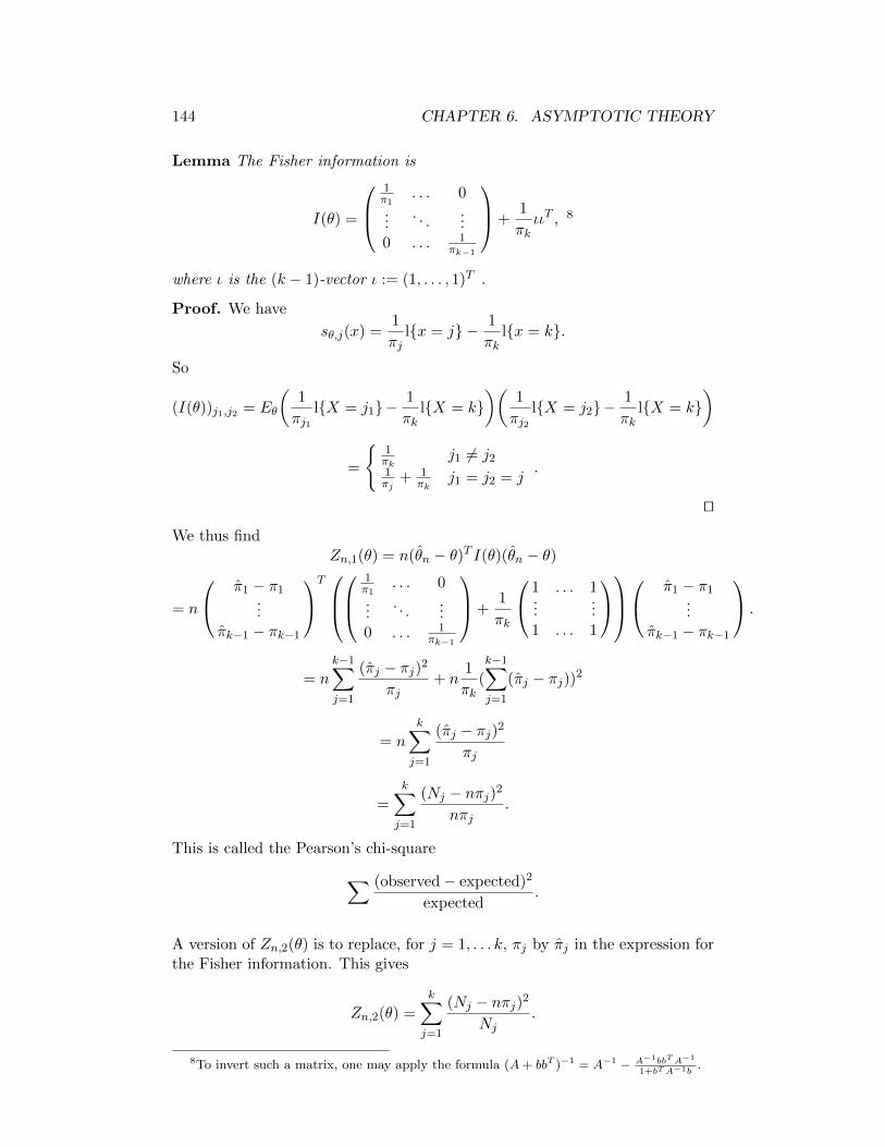
144 CHAPTER 6. ASYMPTOTIC THEORY
Lemma The Fisher information is
I(θ) =
1π1
. . . 0...
. . ....
0 . . . 1πk−1
+1
πkιιT , 8
where ι is the (k − 1)-vector ι := (1, . . . , 1)T .
Proof. We have
sθ,j(x) =1
πjlx = j − 1
πklx = k.
So
(I(θ))j1,j2 = Eθ
(1
πj1lX = j1−
1
πklX = k
)(1
πj2lX = j2−
1
πklX = k
)
=
1πk
j1 6= j21πj
+ 1πk
j1 = j2 = j.
tu
We thus findZn,1(θ) = n(θn − θ)T I(θ)(θn − θ)
= n
π1 − π1...
πk−1 − πk−1
T
1π1
. . . 0...
. . ....
0 . . . 1πk−1
+1
πk
1 . . . 1...
...1 . . . 1
π1 − π1
...πk−1 − πk−1
.
= nk−1∑j=1
(πj − πj)2
πj+ n
1
πk(k−1∑j=1
(πj − πj))2
= n
k∑j=1
(πj − πj)2
πj
=k∑j=1
(Nj − nπj)2
nπj.
This is called the Pearson’s chi-square∑ (observed− expected)2
expected.
A version of Zn,2(θ) is to replace, for j = 1, . . . k, πj by πj in the expression forthe Fisher information. This gives
Zn,2(θ) =k∑j=1
(Nj − nπj)2
Nj.
8To invert such a matrix, one may apply the formula (A+ bbT )−1 = A−1 − A−1bbTA−1
1+bTA−1b.
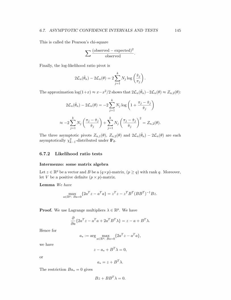
6.7. ASYMPTOTIC CONFIDENCE INTERVALS AND TESTS 145
This is called the Pearson’s chi-square∑ (observed− expected)2
observed.
Finally, the log-likelihood ratio pivot is
2Ln(θn)− 2Ln(θ) = 2k∑j=1
Nj log
(πjπj
).
The approximation log(1+x) ≈ x−x2/2 shows that 2Ln(θn)−2Ln(θ) ≈ Zn,2(θ):
2Ln(θn)− 2Ln(θ) = −2
k∑j=1
Nj log
(1 +
πj − πjπj
)
≈ −2k∑j=1
Nj
(πj − πjπj
)+
k∑j=1
Nj
(πj − πjπj
)2
= Zn,2(θ).
The three asymptotic pivots Zn,1(θ), Zn,2(θ) and 2Ln(θn) − 2Ln(θ) are eachasymptotically χ2
k−1-distributed under IPθ.
6.7.2 Likelihood ratio tests
Intermezzo: some matrix algebra
Let z ∈ Rp be a vector and B be a (q×p)-matrix, (p ≥ q) with rank q. Moreover,let V be a positive definite (p× p)-matrix.
Lemma We have
maxa∈Rp: Ba=0
2aT z − aTa = zT z − zTBT (BBT )−1Bz.
Proof. We use Lagrange multipliers λ ∈ Rp. We have
∂
∂a2aT z − aTa+ 2aTBTλ = z − a+BTλ.
Hence fora∗ := arg max
a∈Rp: Ba=02aT z − aTa,
we havez − a∗ +BTλ = 0,
ora∗ = z +BTλ.
The restriction Ba∗ = 0 gives
Bz +BBTλ = 0.
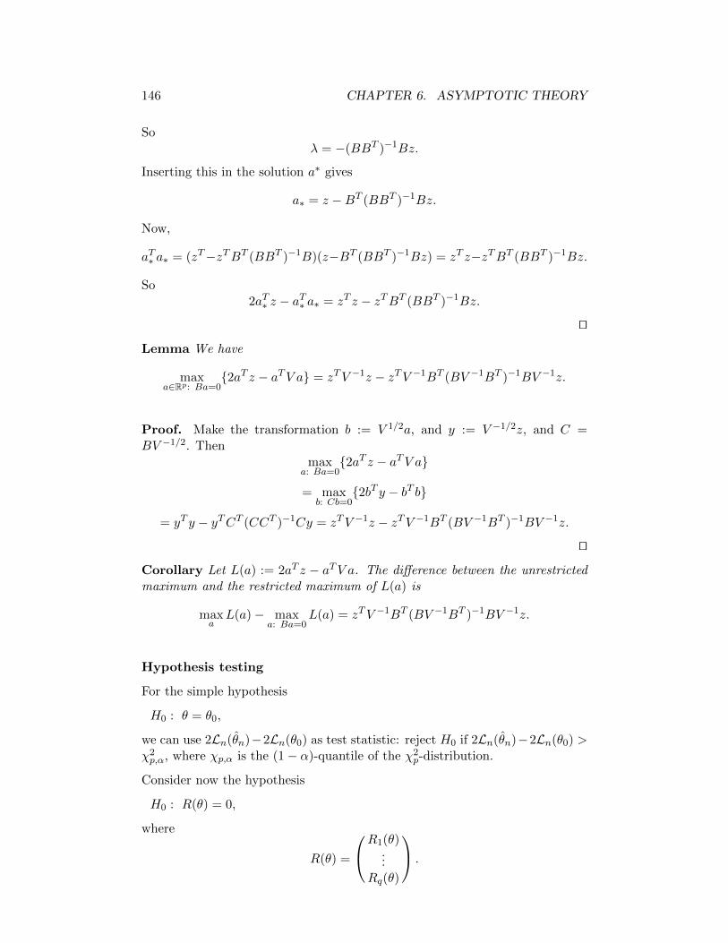
146 CHAPTER 6. ASYMPTOTIC THEORY
Soλ = −(BBT )−1Bz.
Inserting this in the solution a∗ gives
a∗ = z −BT (BBT )−1Bz.
Now,
aT∗ a∗ = (zT−zTBT (BBT )−1B)(z−BT (BBT )−1Bz) = zT z−zTBT (BBT )−1Bz.
So2aT∗ z − aT∗ a∗ = zT z − zTBT (BBT )−1Bz.
tu
Lemma We have
maxa∈Rp: Ba=0
2aT z − aTV a = zTV −1z − zTV −1BT (BV −1BT )−1BV −1z.
Proof. Make the transformation b := V 1/2a, and y := V −1/2z, and C =BV −1/2. Then
maxa: Ba=0
2aT z − aTV a
= maxb: Cb=0
2bT y − bT b
= yT y − yTCT (CCT )−1Cy = zTV −1z − zTV −1BT (BV −1BT )−1BV −1z.
tu
Corollary Let L(a) := 2aT z − aTV a. The difference between the unrestrictedmaximum and the restricted maximum of L(a) is
maxa
L(a)− maxa: Ba=0
L(a) = zTV −1BT (BV −1BT )−1BV −1z.
Hypothesis testing
For the simple hypothesis
H0 : θ = θ0,
we can use 2Ln(θn)−2Ln(θ0) as test statistic: reject H0 if 2Ln(θn)−2Ln(θ0) >χ2p,α, where χp,α is the (1− α)-quantile of the χ2
p-distribution.
Consider now the hypothesis
H0 : R(θ) = 0,
where
R(θ) =
R1(θ)...
Rq(θ)
.
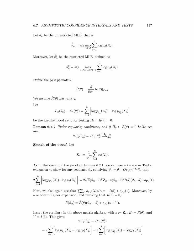
6.7. ASYMPTOTIC CONFIDENCE INTERVALS AND TESTS 147
Let θn be the unrestricted MLE, that is
θn = arg maxϑ∈Θ
n∑i=1
log pϑ(Xi).
Moreover, let θ0n be the restricted MLE, defined as
θ0n = arg max
ϑ∈Θ: R(ϑ)=0
n∑i=1
log pϑ(Xi).
Define the (q × p)-matrix
R(θ) =∂
∂ϑTR(ϑ)|ϑ=θ.
We assume R(θ) has rank q.
Let
Ln(θn)− Ln(θ0n) =
n∑i=1
[log pθn(Xi)− log pθ0n
(Xi)
]be the log-likelihood ratio for testing H0 : R(θ) = 0.
Lemma 6.7.2 Under regularity conditions, and if H0 : R(θ) = 0 holds, wehave
2Ln(θn)− 2Ln(θ0n)
Dθ−→χ2q .
Sketch of the proof. Let
Zn :=1√n
n∑i=1
sθ(Xi).
As in the sketch of the proof of Lemma 6.7.1, we can use a two-term Taylorexpansion to show for any sequence ϑn satisfying ϑn = θ +OIPθ(n
−1/2), that
2n∑i=1
[log pϑn(Xi)−log pθ(Xi)
]= 2√n(ϑn−θ)TZn−n(ϑn−θ)2I(θ)(ϑn−θ)+oIPθ(1).
Here, we also again use that∑n
i=1 sϑn(Xi)/n = −I(θ) + oIPθ(1). Moreover, bya one-term Taylor expansion, and invoking that R(θ) = 0,
R(ϑn) = R(θ)(ϑn − θ) + oIPθ(n−1/2).
Insert the corollary in the above matrix algebra, with z := Zn, B := R(θ), andV = I(θ). This gives
2Ln(θn)− 2Ln(θ0n)
= 2n∑i=1
[log pθn(Xi)− log pθ(Xi)
]− 2
n∑i=1
[log pθ0n
(Xi)− log pθ(Xi)
]
148 CHAPTER 6. ASYMPTOTIC THEORY
= ZTn I(θ)−1RT (θ)
(R(θ)I(θ)−1R(θ)T
)−1
R(θ)I(θ)−1Zn + oIPθ(1)
:= YTnW
−1Yn + oIPθ(1),
where Yn is the q-vector
Yn := R(θ)I(θ)−1Zn,
and where W is the (q × q)-matrix
W := R(θ)I(θ)−1R(θ)T .
We know that
ZnDθ−→N (0, I(θ)).
Hence
YnDθ−→N (0,W ),
so that
YTnW
−1YnDθ−→χ2
q .
tu
Corollary 6.7.1 From the sketch of the proof of Lemma 6.7.2, one sees thatmoreover (under regularity),
2Ln(θn)− 2Ln(θ0n) ≈ n(θn − θ0
n)T I(θ)(θn − θ0n),
and also
2Ln(θn)− 2Ln(θ0n) ≈ n(θn − θ0
n)T I(θ0n)(θn − θ0
n).
Example 6.7.2 Let X be a bivariate label, say X ∈ (j, k) : j = 1, . . . , r, k =1, . . . , s. For example, the first index may correspond to sex (r = 2) and thesecond index to the color of the eyes (s = 3). The probability of the combination(j, k) is
πj,k := Pθ
(X = (j, k)
).
Let X1, . . . , Xn be i.i.d. copies of X, and
Nj,k := #Xi = (j, k).
From Example 6.7.1, we know that the (unrestricted) MLE of πj,k is equal to
πj,k :=Nj,k
n.
We now want to test whether the two labels are independent. The null-hypothesis is
H0 : πj,k = (πj,+)× (π+,k) ∀ (j, k).
6.8. COMPLEXITY REGULARIZATION (TO BE WRITTEN) 149
Here
πj,+ :=
s∑k=1
πj,k, π+,k :=
r∑j=1
πj,k.
One may check that the restricted MLE is
π0j,k = (πj,+)× (π+,k),
where
πj,+ :=
s∑k=1
πj,k, π+,k :=
r∑j=1
πj,k.
The log-likelihood ratio test statistic is thus
2Ln(θn)− 2Ln(θ0n) = 2
r∑j=1
s∑k=1
Nj,k
[log
(Nj,k
n
)− log
(Nj,+N+,k
n2
)]
= 2r∑j=1
s∑k=1
Nj,k log
(nNj,k
Nj,+N+,k
).
Its approximation as given in Corollary 6.7.1 is
2Ln(θn)− 2Ln(θ0n) ≈ n
r∑j=1
s∑k=1
(Nj,k −Nj,+N+,k/n)2
Nj,+N+,k.
This is Pearson’s chi-squared test statistic for testing independence. To findout what the value of q is in this example, we first observe that the unrestrictedcase has p = rs − 1 free parameters. Under the null-hypothesis, there remain(r − 1) + (s− 1) free parameters. Hence, the number of restrictions is
q =
(rs− 1
)−(
(r − 1) + (s− 1)
)= (r − 1)(s− 1).
Thus, under H0 : πj,k = (πj,+)× (π+,k) ∀ (j, k), we have
n
r∑j=1
s∑k=1
(Nj,k −Nj,+N+,k/n)2
Nj,+N+,k
Dθ−→ χ2(r−1)(s−1).
6.8 Complexity regularization (to be written)

150 CHAPTER 6. ASYMPTOTIC THEORY

Chapter 7
Literature
• J.O. Berger (1985) Statistical Decision Theory and Bayesian AnalysisSpringerA fundamental book on Bayesian theory.
• P.J. Bickel, K.A. Doksum (2001) Mathematical Statistics, Basic Ideas andSelected Topics Volume I, 2nd edition, Prentice HallQuite general, and mathematically sound.
• D.R. Cox and D.V. Hinkley (1974) Theoretical Statistics Chapman andHallContains good discussions of various concepts and their practical meaning.Mathematical development is sketchy.
• A. DasGupta (2011) Probability for Statistics and Machine Learning,SpringerContains all the probability theory background needed. (Look out for theupcoming book Statistical Theory, a Comprehensive Course by the sameauthor.)
• J.G. Kalbfleisch (1985) Probability and Statistical Inference Volume 2,SpringerTreats likelihood methods.
• L.M. Le Cam (1986) Asymptotic Methods in Statistical Decision TheorySpringerTreats decision theory on a very abstract level.
• E.L. Lehmann (1983) Theory of Point Estimation WileyA “klassiker”. The lecture notes partly follow this book
• E.L. Lehmann (1986) Testing Statistical Hypothesis 2nd edition, WileyGoes with the previous book.
• J.A. Rice (1994) Mathematical Statistics and Data Analysis 2nd edition,Duxbury PressA more elementary book.
151
152 CHAPTER 7. LITERATURE
• M.J. Schervish (1995) Theory of Statistics SpringerMathematically exact and quite general. Also good as reference book.
• R.J. Serfling (1980) Approximation Theorems of Mathematical StatisticsWileyTreats asymptotics.
• A.W. van der Vaart (1998) Asymptotic Statistics Cambridge UniversityPressTreats modern asymptotics and e.g. semiparametric theory
• L. Wasserman (2004) All of Statistics. A Concise Course in StatisticalInference Springer.Contains a wide range of topics in mathematical statistics and machinelearning.


