Mathematics Behind Planimeters by Osman Yardimci A thesis submitted to the Graduate Faculty of Auburn University in partial fulfillment of the requirements for the Degree of Master of Science Auburn, Alabama Aug 3, 2013 Keywords: Planimeter, Green theorem, Guldin-Pappus theorem Approved by Andras Bezdek, Chair, C. Harry Knowles Professor of Mathematics Narendra Kumar Govil, Alumni Professor of Mathematics and Statistics Wlodzimierz Kuperberg, Professor of Mathematics and Statistics
Transcript
Mathematics Behind Planimeters
by
Osman Yardimci
A thesis submitted to the Graduate Faculty ofAuburn University
in partial fulfillment of therequirements for the Degree of
Master of Science
Auburn, AlabamaAug 3, 2013
Keywords: Planimeter, Green theorem, Guldin-Pappus theorem
Approved by
Andras Bezdek, Chair, C. Harry Knowles Professor of MathematicsNarendra Kumar Govil, Alumni Professor of Mathematics and Statistics
Wlodzimierz Kuperberg, Professor of Mathematics and Statistics
Abstract
Original master thesis project: By studying the literature, collect and write a survey
paper on the mathematics of the planimeters. Planimeter is a somewhat forgotten ingenious
device which was invented in 1814 to satisfy the area computational need of land surveyors
and other real life applications. The project also asked for filling in details of published
proofs and asked for including, if possible, some new statements and generalizations.
On the importance of planimeters: The history of approximating and computing
areas goes back to 3000 BC, when the ancient Egyptians approximated the area of circles.
A great deal of knowledge on areas was summarized by Euclid around 300 BC in his book
entitled Elements. Undoubtedly the discovery of modern time calculus by Newton and Leib-
nitz around 1660 was the biggest advancement in area computation. At the beginning of the
18th century, practical mechanical tools, called planimeters, were patented for determining
the area closed regions.
The following are the outcomes of the thesis: 8 papers ([1], [2], [3], [4], [5],
[6], [7], [8])were included in this review. The mathematics of both of the linear and the
polar planimeters were studied. All arguments were based on Green’s theorem, on the Area
Difference Theorem, and on the theorems concerning sweeping line segments. These theorems
are explained in the first half of the thesis. It turned out that there are two basic approaches
at proving the correctness of planimeters. The section which explains the indirect approach
(using Green’s theorem without computing the involved integrals) is based on a work of B.
Casselman [4]. The section which explains the direct approach (using Green’s theorem with
computing the involved integrals) is based on the work of Ronald W. Gatterdam, [1]. The
explicit approach in the paper of Gatterdam was explained when the two arms of the polar
ii
planimeter had equal length. Using the method of Gatterdam, I verified the correctness of
the polar planimeter in case the arms had different lengths.
iii
Acknowledgments
I would like to acknowledge my advisor Andras Bezdek for his tireless support. I also
would like thank professors, Narendra Kumar Govil and Wlodzimierz Kuperberg for their
willingness to serve on my master committee.
Without the generous financial support of the republic of Turkey government and es-
pecially that of the current prime minister, Recep Tayyip Erdogan, I would not be able to
attend the mathmatics program at Auburn University.
Special thanks go for my friend Olcay Ciftci and his family. They always encouraged
me and were willing to help me at various stages of my career.
The last but the greatest thank goes to my parents, Resat and Rahime Yardimci and
to my wife, Gonul, and to my siblings, Ayse, Fatma and Cevat. Throughout all my life I
Actually if we carefully consider the direction of the octagon we will see that we have
an easy way to decide which triangles will be substracted i.e. we need to calculate only each
triangle’s area by the direction of the common edge with the octagon and then sum all the
results. This process can be done for all simple polygons and their area can be found by
equation (∗).
7
Chapter 3
Planimeters
How can one measure area of two-dimensional shapes, such as leaves, foot soles or bird’s
wings? This question was studied at the beginning of the 19th century and was answered by a
mechanical measuring device called planimeter. Planimeters were designed to determine the
exact areas of shapes drawn on a photo or on a sheet of paper. The first planimeter concept
is attributed to Johann Martin Hermann, Germany, 1814. However the first prototype
was built by the Swiss mathematician Jakob Amsler-Laffon only in 1856. Today, most of
planimeters are digital tools.
The best known planimeters are the linear and the polar planimeters. The latter is also
known as the Amsler planimeter.
3.1 Discription of the Linear Planimeter
The main component of the linear planimeter is the tracer arm (Figure 3.1). One of
its ends is called a pivot and moves only on a straight line (tracer line), as forward and
backward, and the other end is the tracer, which traces out a curve counter clockwise.
During the motion, the arm freely rotates on the pivot. There is a measuring wheel attached
to the tracer arm that rolls during the motions of the tracer while a dial stays in contact
with the wheel and records how much the total rolling of the wheel is.
8
Tracer line
Tracer arm
Tracer
Wheel
Dial
P ivot
Figure 3.1 Technical drawing of the linear planimeter
The linear planimeter measures the total rolling of the wheel by tracing the boundary of
a measured region at the counterclockwise direction. Note that in mathematics the counter-
clockwise direction is defined as positive direction. Since the tracer arm’s length t is a given
constant, the tracer can reach a point which must be at most a distance t from the tracer
line. We will require that no point of the curve is exactly at a distance t from the tracer line.
We can assume that throughout tracing the tracer arm forms an angle θ with the tracer line
which is less than 90◦. So the angle θ is −90◦ < θ < 90◦. (θ is negative if the tarcer point is
on the left from the tracer line and is positive otherwise.) (Figure 3.2).
Tracer line
Tracer armθ◦
Figure 3.2 The reachable region of the linear planimeter and −90◦ < θ◦ < 90◦
9
3.2 Description of the Polar Planimeter
The polar planimeter, in addition to the tracer arm, has a pole and a polar arm. The
pole point is fixed outside of the region enclosed by the curve, and it is joined to the tracer
arm through the polar arm. The polar arm rotates freely on the pole. The other end of
the polar arm, called pivot, joins the polar and the tracer arms together, and they rotate
easily on the pivot. The other end of the tracer arm, called tracer, is designed to trace out
the curve counter clockwise. Similarly to the linear planimeter, the tracer arm of the polar
planimeter has a wheel and a dial.
Pivot
Polar arm
Tracer arm
WheelDial Tracer
Pole
Figure 3.3 Technical drawing of the polar planimeter
Pivot
Pole
Tracer arm
Polar arm
Wheel Dial
Tracer
Figure 3.4 The polar planimeter
10
The polar planimeter, like the linear planimeter, measures the total rolling of the wheel
when a closed curve is traced out counter clockwise. The lengths of the polar and of the
tracer arms are restricted and the former length l is longer than the latter length t. Therefore,
the planimeter cannot reach outside of the circle of radius l+ t and points inside of the circle
of radius l − t. The curve which will be traced must lie in the anulus which is formed by
intersection of the interior of the circle, radius l+ t and the exterior of the circle, radius l− t
(Figure3.4).
Pivot
Pole
Tracer
l
t
Figure 3.5 Traceable anulus area
In order to avoid any confusion, we want to determine uniquely the positions of the
polar and tracer arms in the annulus for each point of the curve. Hence first we define the
angle between the polar arm and the tracer arm as (0◦ < α◦ < 360◦), the angle of the
11
counter-clockwise rotation around the pivot which takes the polar over the tracer arms. The
position of the pivot is uniquely determined if we require that the angle α is 0◦ < α < 180◦.
Furthermore, for some critical reasons, which will be explained in the following sections, the
pole must be outside of the region enclosed by the curve.
As it is seen in Figure 3.5, once the pivot is in the required position than it automatically
remains in the required position as the tracer traces the curve.
(a, b)(x1, y1)
(x2, y2)Pivot
Pole
Tracer
l
t
(x1, y1) 6= (x2, y2)
t2 = (a− x1)2 + (b− y1)
2 = (a− x2)2 + (b− y2)
2
l2 = x12 + y1
2 = x22 + y2
2
Figure 3.6 To uniquely determine the position of the tracer on the curve, the angle betweenthe polar and the tracer arm must be less than 180◦ and more than 0◦
Understanding the theory behind the planimeters depends on a good understanding of
the total rolling of a wheel during shifting and rotating a line which has an attached wheel
whose axis is parallel to the line. It will turn out that the area of a closed curve is equal to
12
the total rolling times the length of the tracer arm. In the next section the total rolling of
the measureing wheel will be discussed.
3.3 Total Rolling of the Planimeters Measuring Wheel and the Swept Area
In this section we study the motion of the tracer arm (and the wheel attached to the
tracer arm) independently from the rest of the mechanics and the swept area. Here the
tracer arm is just a segment with a wheel attached to it.
Let us start with a simple observation. If the axis of the measuring wheel is perpen-
diculuar to the path throughout the entirely motion, then the measuring wheel totally rolls
an angle θ =P
R, where P is a distance and R is the wheel’s radius (Firgure 3.7).
a
aθR
︸ ︷︷ ︸
θ = PR
P = θR
Figure 3.7 The total rolling of the measuring wheel.
Therefore the rotation of the wheel is related to the traced path, but this relation is a
bit subtle, especially if we want to understand its connection to the area swept by the tracer
arm. In the rest of this section we consider a line segment that has a measuring wheel whose
axis is parallel to it.
We will use the following notations: Γ denotes the path traversed by the center of the
wheel and−→N denotes the normal unit vector of the line segment and
−→T denotes the unit
direction vector of the path Γ at each point.
Theorem 3.1. During a motion of the segment on curve Γ, total rolling of the wheel is equal
to ˆΓ
−→N · −→T ds
13
If the segment moves perpendiculary to itself a distance s, then−→T =
−→N and the mea-
suring wheel rolls a distance s; furthermore, the swept area is ls, where the segment’s length
is l (Figure 3.8).
NT
Γ
ds
lWheelFigure 3.8 The swept area is ls.
However, if the line segment is shifted on a line segment, then the wheel rotates a
distance h which is the height of the parallelogram and the swept area is equal to hl (Figure
3.9).
NT
Γ
ds
lWheel
h
Figure 3.9 The swept area is hl.
If the line parallelly moves on itself then, the wheel will not roll at all, so the swept area
is equal to 0 (Figure 3.10).
14
n
t
︷ ︸︸ ︷
︸ ︷︷ ︸
Γ
ds
Figure 3.10 The line parallel moves on itself then the area is 0.
From the above results, when a segment is translated, the swept area directly depends
on the distance P , which is measured by the wheel and the length l of the segment.
In all cases, the total rolling of the wheel basically depends on the magnitudes of the
unit vectors−→T and
−→N at each point of the path. Therefore, in the first case, since
−→N ‖−→T , the
dot product−→N ·−→T = 1, then the moved distance of the wheel is exactly equal to the length
of the traced path. In the second case, the vectors−→N and
−→T are neither parallel (
−→N ∦−→T )
nor perpendicular (−→N 6⊥−→T ), and so the dot product
−→N ·−→T is equal to l times the height h of
the parallelogram. In the third case, the vectors−→N and
−→T are perpendicular i.e. (
−→N⊥−→T ),
therefore−→N ·−→T = 0.
NT
(a)−→N ‖−→T , then
−→N ·−→T = 1.
N Tα
(b)−→N ∦−→T and
−→N 6⊥−→T , then
−→N ·−→T =
cosα.
N T
(c)−→N⊥−→T , then
−→N ·−→T = 0.
15
Therefore, when the motion of the line is parallel to itself, then the total distance
measured by the wheel P is equal to´ −→N ·−→T ds. Actually this basic result is valid for general
motions because they can be approximated by a sequence of rotations and translations.
NT
a
b
c
Figure 3.12 A motion is formed by rotation and parallel shifting. (−→N ∦−→T )
Infinitesimally, the distance which is displayed on the dial, while it moves from a to c is
equal to the distances which are displayed when it moves from a to b and from b to c so
P =
ˆ −→N ·−→T ds
−→N
−→T
Γ
ds
Wheel
Figure 3.13 General case, the total distance measured P =´ −→N ·−→T ds.
16
We already saw that in cases of various parallel line motions the swept area is equal to
the product of the total rolling of the wheel and the length of the line segment. However,
this is not true for general motions unless the wheel is attached at the middle of the segment.
In the next section, Guldin-Pappus theorem is given, which shows how to calculate the area
in terms of the rotation of the wheel and the length of the segment in case of non-parallel
motions.
Assume we have a plane curve C and an external segment l in the plane.
Theorem 3.2 (Guldin-Pappus Theorem (1641)). If the curve revolves about the line then
the surface area of the solid of the revolution is equal to the length of the curve times the
circumference of the circle obtained by the rotating which passes through the centroid of the
curve along the line.
Here, we do not give the proof but the relation of the line sweeping and the area is
explained.
Suppose that the wheel of radius R is attached at the middle of the line segment. Then,
if the wheel rolls an angle θ at the end of the motion, the measuring wheel rolls a distance
P = Rθ and so the swept area by the segment is Pl.
Figure 3.14 The wheel is attached at the middle of the segment.
17
If we infinitesimally partition the swept area as shown above, then we get the strips
below.
Figure 3.15 An infinitesimal strip.
For each of the strips, when the upper line is rotated to make it parallel to the bottom
line as in Figure 3.15, the wheel does not roll because it is at the middle of the line. Moreover,
for an infinitesimal partition, the area is not changed because the area lost to the right of
the midpoint is equal to the area gained to the left from the midpoint. Applying the same
argument for each strip, then we get a combination of parallel line motions (Figure 3.16).
Figure 3.16 An infinitesimal band.
As in seen in Figure 3.17, if we horizontally slide the right side of the swept area to the
left, the measuring wheel does not roll because the motion is paralel to its axis and the area
is not change.
18
Figure 3.17 The horizontal motion.
Then, the swept area can be turned into a cylinder and its surface area is the length
of the segment times the total rolling of the measuring wheel i.e. total swept area is Pl. (
Figure 3.18.) Therefore the theorem is verified for the line segment sweeping.
Figure 3.18 Making cylinder.
However, during the parallelization process, one end of the line goes up and the other
goes down. In general, this fact will be considered a signed interpretation.
This result is valid when the wheel is at the middle of the line. However one might
wonder what will happen if the wheel is placed somewhere else of the line.
Let the wheel be far away from the middle of the segment and its position vector at
time t be −→v (t) +−→c (t) where −→c (t) is the middle point of the segment and −→v (t) is a vector
which lies on the segment with a fixed length λ (Figure3.19). The wheel traces a curve Γ(t)
Figure 3.19 For the general position of the wheel during the general motion of the segment.
Let us recall that P =´
Γ
−→N ·−→T ds. Here, the unit direction vector
−→T is (x′(t),y′(t))√
x′(t)2+y′(t)2and
the elementary arc length is ds = |Γ′(t)|dt =√x′(t) + y′(t)dt. Therefore;
P =
ˆ
Γ
−→N ·−→T ds
=
ˆ
Γ
−→N · (x′(t), y′(t))√
x′(t)2 + y′(t)2
√x′(t)2 + y′(t)2dt
=
ˆ
Γ
−→N ·(x′(t), y′(t))dt
=
ˆ
Γ
−→N ·(−→c ′(t) +−→v ′(t))dt
=
ˆ
Γ
−→N ·−→c ′(t)dt
︸ ︷︷ ︸1
+
ˆ
Γ
−→N ·−→v ′(t)dt.
︸ ︷︷ ︸2
Here, the integral (1) would be the distance of the wheel’s motion if it were at the middle
of the segment. In the integral (2), since−−→N(t) is the normal vector of the line in which the
vector−−→v(t) lies,
−−→N(t) and
−−→v(t) are perperndicular (
−−→N(t) ⊥ −−→v(t)) (Figure 3.20), the vector
−−→v(t)
travels around a circle of radius λ.
20
t
−−→N(t)
−−→v(t)
Figure 3.20 At each t, the length of −→v is λ and the vectors−→N and −→v are perpendicular.
Thus−−→v(t)′ is parallel to
−→N , and their dot product is the signed length of
−−→v(t)′. Therefore,
the integral (2) is equal to the total rotation of the segment times λ.
Therefore, when the total line rotation is β and the wheel is at distance λ from the
center of the segment, the distance P is measured Pc plus λ times β i.e. P = Pc + λβ where
Pc is the distance that would be measured if the wheel were at the midpoint.
From this general situation, it can be easily seen that when the wheel is at the midpoint
of the segment then the integral (2) is equal to 0 so the total wheel motion would be Pc.
Therefore by Guldin-Pappus theorem, the swept area is equal to
lPc = lP − lλβ.
Theorem 3.3. If a segment’s end points trace two curves ΓA and ΓC as the boundaries of
the regions A and C, respectively, (Figure 3.21 and 3.22) then total swept area is equal to
C − A
21
Proof. Consider the upward motion of the line segment depicted on Figure 3.21. The dot
product of the vectors−→N and
−→T is positive, so the sign of the swept area is positive. The
other way the dot prodcut is negative so the sign of the area is negative Figure 3.22.
A B C
Figure 3.21−→N · −→T > 0
A BC
Figure 3.22−→N · −→T < 0
In the figure, when−→N · −→T is negative, the swept areas A and B have negative signs and
when−→N · −→T is positive, the swept areas B and C have positive signs. Thus, adding them
together yields
−(A+B) + (B + C) = C − A
C−(A)
Figure 3.23 −(A+B) + (B + C) = C − A.
Since during the motion of the line segment the total swept area is lPc = lP − lλγ, we
have C −A = lPc = lP − lλγ. Since the line segment returns to its starting position, so the
total rotation of the line segment γ is zero, and so, C − A = lP .
22
If we could choose the area A to be equal to zero, then the area C would be exactly
equal to the line segmnet’s length l times the distance P measured by the rotation of the
wheel.
In case of the polar planimeter, one end of the polar arm is fixed at the pole and the
other end, called pivot, is connected to the tracer arm and restricted to move on a circle
arc, and thus A = 0. The tracer arm plays the role of the moving segment as the above line
segment and travels on a mesured curve by the tarcer.
Corollary 3.1 For the polar planimeter, if the pole is outside the measured area and the
tracer arm returns to its original position then the total rotating of the tracer arm is zero
and the area is Pl. (Figure 3.24)
C
A
Figure 3.24 The generated region A is a cricular arc.
Here, since, the area of the arc is zero, the area of the closed region is Pl.
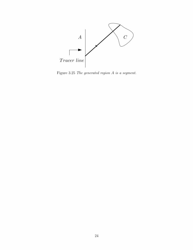
Corollary 3.2 If the tracer of the linear planimeter traces the complete boundary then the
total rotation of the tracer arm is equal to zero and the swept area is Pl
Since the tracer arm returns to the inital position after tracing the simple closed region,
total rotation of tracer arm γ is zero. Since the pivot end moves on the trace line as forward
and backward we have that A = 0 and thus the total area is the length of the tracer times
the total rolling of the measuring wheel (Figure 3.25).
23
CA
Tracer line
Figure 3.25 The generated region A is a segment.
24
Chapter 4
Explaining Planimeters by Green’s Theorem Without Evaluating Integrals
In this chapter we are going to prove the planimeter’s theorem using Green’s theorem.We
will start by Green’s theorem. Then Green’s theorem is applied for the polar and linear
planimeters.
4.1 Green’s Theorem
Let us recall that a curve is simple closed if the curve does not intersect with itself and
closed; it is said to be oriented positively if the boundary C is the counterclockwise oriented;
and it is called piecewise smooth if it is smooth curve with possible finite number of curners.
(Figure 4.1)
R R RC C C
Figure 4.1 Examples of simple closed, positively oriented and piecewise smooth curves, whereR is the interior and C is boundary of the regions.
Theorem 4.1. Let D be a region with the interior R and boundry C which is simple closed,
positively oriented and piecewise smooth and let−→F (x, y) =< P (x, y), Q(x, y) > be a vector
field where P (x, y) and Q(x, y) are functions of two variable and have continuous first order
partial derivative over an open region containing R, then
ffiC
P (x, y)dx+Q(x, y)dy =
ˆ ˆR
(∂Q
∂x− ∂P
∂y
)dA.
25
The integrand Qx − Py is called the curl of the vector field.
Corollary 4.1 If the curl is equal to 1, then the duble integral in Green’s theorem is the
area of the region D, i.e.
ˆ ˆR
(∂Q
∂x− ∂P
∂y
)dA =
ˆ ˆR
dA = area(D).
For example if the vector field F (x, y) =(−y
2,x
2
)then Py = −1
2and Qx =
1
2so
Qx − Py =1
2−(−1
2
)= 1. (Figure 4.2).
y
x
Figure 4.2 The vector fields F (x, y) =(−y
2,x
2
).
If the vector field F (x, y) = (0, x) then Py = 0 and Qx = 1, and so Qx−Py = 1− 0 = 1.
(Figure 4.3).
26
y
x
Figure 4.3 The vector fields F (x, y) = (0, x).
The above examples show us that the vector fields whose line integral on the boundary
of a closed region gives us the area of the region is not uniquely determined. In the next
section, we are going to show that the product of the curl of the vector fields of the planimeter
and the length of the tracer arm is 1.
4.2 An Application of Green’s Theorem for the Polar Planimeter
We have already chosen the tracer’s motion around a closed curve in the positive direc-
tion. Since the region is closed, simple then the tracer follows up the boundary Γ which is
a continuous curve. For each point of the annulus, we have a unit normal vector−→N of the
tracer arm at the tracer which indicates the counterclockwise.
27
−→N
K
L
M
Γ
Figure 4.4 At each point of the annulus there is a normal vector−→N of tracer arm at tracer .
How much does the measuring wheel roll, when the curve is traced along a curve Γ,
depends on the angle between the each point of the normal vector−→N and the tangent vector
−→T of the curve. Figure 4.4 illustrates different possibilities. When the tracer moves a distance
∆s on the curve, at K the wheel responds ∆s; at L the result is between ∆s and 0; and at
M the wheel is not going to roll.
In order to make more clear what is the relation between the measuring wheel’s rolling
and the normal and tangent vectors on the curve, let−→Ni for i = 1, 2...n denote the normal
vectors of tracer arm at a given set of subdivision points of the curve and at these points
let−→Ti be the unit tangent vectors of the curve. Suppose that the tracer travels a distance
∆si from the ith to the (i+ 1)th subdivision point on the boundary Γ, then the wheel rolls
a distance−→Ni ·−→Ti∆si where
−→Ni ·−→Ti is the dot product of the two vectors. Therefore total
rolling of the wheel isn∑
i=1
−→Ni ·−→Ti∆si.
The usual limit process gives that the total rolling of the wheel is equal to
limmax{∆si}→0
∑−→Ni ·−→Ti∆si =
ffiΓ
−→N · −→T ds.
28
Since for a polar planimeter, the angle α between the tracer and polar arms is 0◦ < α <
180◦ the configiration of the planimeter is unique at each point of the annulus. Therefore
for each point of the annulus there is a unique normal vector and these vectors gives us a
vector field and say it−→N (x, y) = (P (x, y), Q(x, y)). Since the studied region’s boundry Γ is
completely included in the annulus where the vector field−→N (x, y) is defined, by the Green’s
theorem, the line integral of−→N on the boundary Γ of the region D is equal to certain double
integral over the interior R of the region of D. Therefore,
ffiΓ
−→N · −→T ds =
ffiΓ
P (x, y)dx+Q(x, y)dy =
ˆ ˆR
(Qx − Py)dA.
As we have mentioned that if the curl Qx − Py is equal to 1 then the line integral is equal
to the area of the region D. In fact, instead of showing the curl Qx − Py is 1, for the polar
planimeter, we are going to show that the vector field t−→N (x, y) verifies the property that its
curl t(Qx − Py) is 1. Normally, the vector field−→N would be found and then its curl would
be detemined. However we do not directly find the vector field and its curl, instead of this
special properties of the vector field will be used to verify that the curl t(Qx − Py) is one.
Then by Green’s theorem,
ffiΓ
t−→N · −→T ds =
ffiΓ
t(P (x, y)dx+Q(x, y))dy
=
ˆ ˆR
t(Qx − Py)dA =
ˆ ˆR
1dA = areaofR.
The vector field−→N has circular symmetry, i.e. in the annulus, the angle between the normal
vectors of the tracer arm and tangent vectors of a circle centered at the pole point is constant.
29
Figure 4.5 The vector field of the polar planimeter has circular symmetry.
By the law of cosines, we get a formula which gives the cosine of the angle between the
line segment from the pole to the tracer and the tracer arm.
l
t
ρ
γ
−→N
Figure 4.6 The circumferential component of−→N .
30
Therefore, by Figure 4.6
l2 = t2 + ρ2 − 2tρ cos(γ)
which gives
cos(γ) =t2 + ρ2 − l2
2tρ
Now, let us define the function f by f(ρ) = cos(γ) =t2 + ρ2 − l2
2tρ.
According to the Green’s theorem the line integral on a closed curve of the path integral
is equal to the area of the region if the curl of the vector field is equal to 1. Here, instead of
directly showing the curl is equal to 1, we show that on an appropriate closed curve in the
annulus the line integral of the vector field times t is the area then this result gives that the
curl is 1. For this we choose a convenient curve Γ. (Figure 4.7)
C1
C2
C3
C4
ρ
∆ρ
∆θ
R
Figure 4.7 A convenient curve Γ with the paths C1, C2, C3 and C4.
Let us show that the area of R is equal to´ ´
Rt(Qx − Py)dA. Let us calculate the line
integral of the vector field−→N along the curve Γ.
ffiΓ
−→N · −→T ds =
ˆC1
−→N · −→T ds+
ˆC2
−→N · −→T ds+
ˆC3
−→N · −→T ds+
ˆC4
−→N · −→T ds
31
Since the vector field has circular symmetry,
ˆC2
−→N · −→T ds = −
ˆC4
−→N · −→T ds.
therefore,
ffiΓ
−→N · −→T ds =
ˆC1
−→N · −→T ds+
ˆC3
−→N · −→T ds
=
ˆC1
f(ρ+ ∆ρ)dθ +
ˆC3
f(ρ)dθ
= ((ρ+ ∆ρ)f(ρ+ ∆ρ)− ρf(ρ))θ
=
((ρ+ ∆ρ)
(ρ+ ∆ρ)2 + t2 − l22t(ρ+ ∆ρ)
− ρρ2 + t2 − l2
2tρ
)θ
=θ
2t((ρ+ ∆ρ)2 − ρ2)
Then t times the path integralfl
Γ
−→N · −→T ds is equal to
θ
2((ρ+ ∆ρ)2− ρ2) which is the area of
the region R and so by the Green’s theorem, we have reached that t(Qx − Py) = 1.
Now, we generalize this result for any simple closed region D in the annulus using
an indirect argument. Let us assume that there is a point (x1, y1) ∈ D which does not
satisfy the result, i.e. t(Qx − Py)(x1, y1) 6= 1. Then without loss generality we can assume
t(Qx − Py)(x1, y1) > 1 and since t(Qx − Py) is a continuous function over the annulus, for a
sufficiently small neighborhood ∆D of the point (x1, y1) the function t(Qx − Py) > 1 and so
ˆ ˆ∆D
t(Qx − Py)dA >
ˆ ˆ∆D
1dA = area of ∆D,
a contraction. So the function t(Qx − Py) is the constant function over the annulus.
Therefore, for any simple, closed region D with boundary Γ, the area is equal to the
length t of the tracer arm times the total rollingfl
Γ
−→N · −→T ds of the measuring wheel in the
annulus, i.e.
area of D = t
ffiΓ
−→N · −→T ds.
32
4.3 An Application of Green’s Theorem to the Linear Planimter
Similarly to the polar planimeter, let Γ be the piecewise continuous boundary curve of
the region D. Assume that the orientation of the tracer’s motion of the linear planimeter
on a closed curve is positive. For each point of the reachable region there is a unit normal
vector−→N of the tracer arm at the tracer that is consistent with the positive direction.
−→N
K
L
M
Figure 4.8 At each point of the reachable region, there is a unit normal vector−→N of tracer
arm at tracer.
The discussion of how much the measuring wheel rolls along the tracing is the same
as that of the polar planimeter’s. The unit vectors−→N and
−→T mean the same as before,
therefore, the total rolling of the wheel isfl
Γ
−→N · −→T ds. The unit normal vectors of the tracer
arm at each point of the reachable region form a vector field−→N (x, y). In the vector fields,
the vectors on a straight line which is parallel to the tracer line form a vector band that is
parallel to the tracer line, i.e. the vectors in a band are parallel to each other. (Figure 4.9)
33
Figure 4.9 The unit normal vectors of the tracer arm form parallel bands to the tracer line.
As the properties of the vector field of the polar planimeter were considered to show
that the total wheel measuring times the tracer arm’s length is the area, here the properties
of the vector field associated with the linear planimeter will be considered.
In the (x, y) coorditate system, let the axis y be the tracer line and let γ be the angle
between the tracer line and the trace arm.
(x, y)
(0, Y )
−→N
y
x
tγ
Figure 4.10 The y axis is the tracer line.
Let us define the function f by f(x) = sin(γ) =x
tand let us choose an appropriatel
region D with the boundary Γ to show that the integrand t(Qx − Py) = 1. (Figure 4.11)
34
(x + ∆x, y + ∆y)
(x + ∆x, y)(x, y)
(x, y + ∆y)
C1
C2
C3
C4
∆Γ
Figure 4.11 An appropriate rectangle bounded by the directed segments C1, C2, C3 and C4.
Using Green’s theorem, we are going to show that the area of the rectangle R is equal
to´ ´
Rt(Qx − Py)dA. We start by calculating the line integral of the vector field t
−→N (x, y)
over the boundary Γ.
ffiΓ
−→N · −→T ds =
ˆC1
−→N · −→T ds+
ˆC2
−→N · −→T ds+
ˆC3
−→N · −→T ds+
ˆC4
−→N · −→T ds.
The line integrals over the paths C2 and C4 are just different by sign. To see this, let us
calculate the dot product−→N ·−→T for the points (x1, y+∆y) and (x1, y) where x1 ∈ (x, x+ ∆x)
in Figure 4.12 ,
35
C4
C2
C1
C3
−→N
−→T
y
x
y
y + ∆y
x x+ ∆x
θ
π2 − θ
π2 + θ
x1
Figure 4.12 Understanding the dot product of−→N and
−→T over the paths C2 and C4.
We have
−→N (x1, y + ∆y) · −→T (x1, y + ∆y) = cos(
π
2+ θ) = − cos(
π
2− θ) = −−→N (x1, y) · −→T (x1, y)
Since every point of (x, x + ∆x) gives this result, we have´C2
−→N · −→T ds +
´C4
−→N · −→T ds = 0,
and so the line integral is equal to the line integral over the paths C1 and C3 i.e.
ffiΓ
−→N · −→T ds =
ˆC1
−→N · −→T ds+
ˆC3
−→N · −→T ds
=
ˆC1
f(x+ ∆x)ds+
ˆC3
−f(x)ds
=x+ ∆x
t
ˆC1
ds− x
t
ˆC3
ds
= (x+ ∆x
t− x
t)∆y =
∆x∆y
t.
36
Then, if we multiply the line integral with the length of the tracer arm t, we get the area of
the rectangle i.e.
t
ffiΓ
−→N · −→T ds = ∆x∆y,
and also by the Green’s theorem we have
t
ffiΓ
−→N · −→T ds =
ˆ ˆR
t(Qx − Py)dA.
Thus the integral´ ´
Rt(Qx − Py)dA is the area of R whenever R is an axis paralel
rectangle and the curl t(Qx − Py) of the vector field t−→N (x, y) is 1. Indeed if there is a point
(x′, y′) in the reachable region such that t(Qx − Py)(x′, y′) 6= 1, then without loss generality
we can assume t(Qx − Py)(x′, y′) > 1. Since the function t(Qx − Py)(x, y) is continuous, we
can choose a sufficiently small axis rectangle ∆D around the point (x′, y′) so that over the
neighborhood t(Qx − Py)(x, y) > 1. Then
ˆ ˆ∆D
t(Qx − Py)dA >
ˆ ˆ∆D
1dA = area of ∆D
which contradicts that´ ´
∆Dt(Qx − Py)dA is the area of the region. Thus for any point of
the reachable region the function value of t(Qx − Py) is equal to 1.
Finally this implies that the area of any simple closed region D in the reachable area is
equal to the total wheel rolling along the boundary Γ of the region times the length of the
tracer arm i.e.
t
ffiΓ
−→N · −→T ds =
ˆ ˆD
t(Qx − Py)dA =
ˆ ˆD
1dA = area of D.
37
Chapter 5
Explaining Planimeters by Green’s Theorem With Evaluating Integrals
In this chapter, the working of the planimeters are explained by the direct use of the
Green’s Theorem.
5.1 The Direct Use of Green’s Theorem for the Polar Planimeter
In the xy-coordinate system, the pole point is fixed at the origin, OA and AB are the
polar and tracer arms with lengths l and t, respectively.
r
t
l
D
Γ
O
A
B
y
x
dN
dN
dT
ldφ
αθφ
γ
α+ γ
Figure 5.1 The mechanics of the polar planimeter.
38
The measuring wheel is attached to the tracer arm at A so that its axis is parallel to
the tracer arm. We assume that the planimeter traces, by the tracer at B, the boundary Γ
of a region D in a counterclockwise direction. The motion of the tracer forces the pivot to
move on the circle with center O and radius l. Notice again that the wheel rolls only if the
motion is not parallel to the axis of the wheel.
We are going to show that the total rolling of the measuring wheel times the length of
the tracer arm is the area of a measured region D.
During the motion, the tracer arm has two elementary motions: translation and rotation.
When the tracing is completed, the terminating position of the tracer arm is the same as
the initial position so total rotation of the tracer arm is zero and the rotation does not affect
the total rolling of the wheel. Therefore, we consider only the translation.
Consider Figure 5.1, which illustrates that the tracer starts to move at point (x, y) and
takes a directed distance ∆B on the curve Γ. Let ∆N be a component of ∆B perpendicular
to the tracer arm, let ∆φ be the infinitesimal change of the angle φ. The pivot covers a
distance l∆φ and the component ∆N becomes equal to cos(α + γ)l∆φ. During the motion,
the rotation of tracer arm is equal to ∆β but that is not changing the pivot’s position so the
wheel does not roll. Therefore for an infinitesimal travel ∆B of the tracer, the wheel rotates
∆N = cos(α + β)l∆φ. Using a standard subdivision and limit argument we get
Total wheel rolling =
ffiΓ
dN = lim∆B→0
lcos(α + γ)∆φ =
ffiΓ
lcos(α + γ)dφ
Here, we are going to write the component dN = P (x, y)dx + Q(x, y)dy and apply
Green’s theorem, i.e.
ffiΓ
dN =
ffiΓ
P (x, y)dx+Q(x, y) =
ˆ ˆD
(Qx − Py)dA,
then show that ˆ ˆD
(Qx − Py)dA =1
t
ˆ ˆD
dA.
39
Let us find, P (x, y) and Q(x, y). Since dN = cos(α + γ)ldφ let us calculate cos(α+ γ),
using one of the trigonometries identities.
cos(α + γ) = cos(α) cos(γ)− sin(α) sin(γ).
1
t2+r2−l2
2tr
γ
Figure 5.2 The computationof sin γ.
In view of Figure 5.1, from the triangle OAB
l2 = t2 + r2 − 2tr cos γ
so cos γ =t2 + r2 − l2
2tr
Also we can easily find
sin γ =
√1−
(t2 + r2 − l2
2tr
)2
=
√−t4 − r4 − l4 + 2t2r2 + 2t2l2 + 2r2l2
2tr.
Similarly,
cosα =l2 + r2 − t2
2lrand sinα =
√−t4 − r4 − l4 + 2t2r2 + 2t2l2 + 2r2l2
2lr.
Therefore,
cos(α + γ) = cos(α) cos(γ)− sin(α) sin(γ)
=
(l2 + r2 − t2
2lr
)(t2 + r2 − l2
2tr
)
−(√−t4 − r4 − l4 + 2t2r2 + 2t2l2 + 2r2l2
2lr
)(√−t4 − r4 − l4 + 2t2r2 + 2t2l2 + 2r2l2
2tr
)
=r4 − l4 − t4 + 2l2t2
4r2lt− −t
4 − r4 − l4 + 2t2r2 + 2t2l2 + 2r2l2
4r2tl
=r2 − t2 − l2
2tl.
40
To compute dφ, (Figure 5.1), since
r2 = x2 + y2
and
tan θ =y
x⇒ θ = tan−1(
y
x
so we have
dr =x
rdx+
y
rdy
and
dθ = − y
r2dx+
x
r2dy
Since cosα =t2 + r2 − l2
2tr, the angle α = cos−1
(t2 + r2 − l2
2tr
).
Then, φ = θ + α = θ + cos−1
(t2 + r2 − l2
2tr
), and consequently
dφ = dθ + dα = dθ +−(r2 − l2 + t2)
r√−t4 − r4 − l4 + 2t2r2 + 2t2l2 + 2r2l2
dr.
If we write dr and dθ in the above formula, we get
dφ = dθ +−(r2 − l2 + t2)
r√−t4 − r4 − l4 + 2t2r2 + 2t2l2 + 2r2l2
dr
=(− y
r2dx+
x
r2dy)
+−(r2 − l2 + t2)
r√−t4 − r4 − l4 + 2t2r2 + 2t2l2 + 2r2l2
(xrdx+
y
rdy)
=
(− y
r2+
−x(r2 − l2 + t2)
r2√−t4 − r4 − l4 + 2t2r2 + 2t2l2 + 2r2l2
)dx
+
(x
r2+
−y(r2 − l2 + t2)
r2√−t4 − r4 − l4 + 2t2r2 + 2t2l2 + 2r2l2
)dy.
41
Therefore we obtained dφ and cos(α+γ), and substitutes these values in dN = lcos(α+
γ)dφ we get
dN = lcos(α + γ)dφ
= l
(r2 − t2 − l2
2tl
)(− y
r2+
−x(r2 − l2 + t2)
r2√−t4 − r4 − l4 + 2t2r2 + 2t2l2 + 2r2l2
)dx
+ l
(r2 − t2 − l2
2tl
)(x
r2+
−y(r2 − l2 + t2)
r2√−t4 − r4 − l4 + 2t2r2 + 2t2l2 + 2r2l2
)dy
=
( −x(r2 − t2 − l2)(r2 − l2 + t2)
tr√−t4 − r4 − l4 + 2t2r2 + 2t2l2 + 2r2l2
− y
2t+y(t2 + l2)
r2t
)dx
+
( −y(r2 − t2 − l2)(r2 − l2 + t2)
tr√−t4 − r4 − l4 + 2t2r2 + 2t2l2 + 2r2l2
+x
2t− x(t2 + l2)
r2t
)dy
= P (x, y)dx+Q(x, y)dy.
When f(r) is a differentiable function of r then for the partial derivative of f we have
y∂f
∂x= y
∂f
∂r
∂r
∂x= y
∂f
∂r
x
r= x
∂f
∂r
y
r= x
∂f
∂r
∂r
∂y= x
∂f
∂y
Since f(r) =−(r2 − t2 − l2)(r2 − l2 + t2)
tr√−t4 − r4 − l4 + 2t2r2 + 2t2l2 + 2r2l2
is a differentiable function of r then
y∂f
∂x= x
∂f
∂y
and also direct calculation shows that
∂
∂y
(y(t2 + l2)
r2t
)=
(x2 − y2)
r4
(t2 + r2)
t=
∂
∂x
(−x(t2 + l2)
r2t
).
42
On applying the Green’s theorem to the total rolling of the wheel, we get
ffiΓ
dN =
ffiΓ
P (x, y)dx+Q(x, y) =
ˆ ˆD
(Qx − Py)dA
=
ˆ ˆD
1
2t−(− 1
2t
)dA =
ˆ ˆD
1
tdA.
Therefore total rolling times the length of the tracer arm is the area of the region D,
that is
t
ffiΓ
dN =
ˆ ˆD
dA = area of D.
5.2 The Direct Use of Green’s Theorem for the Linear Planimeter
In the xy−coordinate system, let the y−axis be as the tracer line and AB as the tracer
arm with length t. The measuring wheel is attached at a distance l from the pivot.
y
x
dN
A(0, a)
O
B(x, y)
WheelP ivot
Tracer
αl
Figure 5.3 The mechanics of the linear planimeter.
We are going to show, as it was done for polar planimeter, that the total rolling of the
wheel times the length of the tracer arm is the area of a measured region.
43
Every motion of the tracer can be replaced by a sequence of translations and rotations
of the arm. So an infinitesimal motion ∆B of the tracer on the boundary Γ is the same as
infinitesimal paralel shifting ∆a and rotation ∆θ.
At a rotation, the pivot does not change place, just the arm turns an angle ∆θ on the
pivot and at a translation the arm moves parallelly by a distance ∆a, so the pivot’s new
coordinates are (0, a + ∆a). The components of the motions, which are perpendicular to
the arm, causes the rolling of the wheel. Therefore, since the rotation is perpendicular to
the arm it also affect the rolling, i.e. the wheel rolls a distance l∆θ plus sinα∆a. By the
standard subdivision and limit argument we have
Total rolling =
ffiΓ
dN = lim∆B→0
sinα∆a+ l∆θ =
ffiΓ
sinαda+
ffiΓ
ldθ
After tracing the curve Γ, the tracer arm returns to its initial position, so the rotation
of the arm equals to zero and as it seen in the Figure 5.2 we have sinα =x
t, and so
Total rolling =
ffiΓ
dN =
ffiΓ
sinαda =1
t
ffiΓ
xda. (∗)
To compute da, we have in Figure 5.2,
t2 = x2 + (y − a)2
Because of the initial assumptions of the linear planimeter, the tracer arm cannot rotate
past the roller, thus we have a < y and so a has an unique value for each point (x, y) of the
curve. Then
a = y −√t2 − x2
so da = dy +x√
t2 − x2dx,
44
and and substituting this expression in the (∗) we get
1
t
ffiΓ
xda =1
t
ffiΓ
x
(dy +
x√t2 − x2
dx
)
=1
t
ffiΓ
x2
√t2 − x2
dx+ xdy
=1
t
ffiΓ
P (x, y)dx+Q(x, y)dy.
Now, by taking the partial derivatives of P (x, y) and Q(x, y) with to y and x, we have,
Py = 0 and Qx = 1,
and this on applying Green’s theorem gives
Total rolling =
ffiΓ
dN =1
t
ˆ ˆD
(Qx − Py)dA
=1
t
ˆ ˆD
dA.
Therefore, the computation shows that total rolling times the arm length is the area of
the measured area i.e.
t
ffiΓ
dN = area of D.
45
Bibliography
[1] Ronald W. Gatterdam, ”The Planimeter as an Example of Green’s Theorem”, Mathe-matical Association of America, 88 (Nov, 1981), pp. 701-704.
[2] Henrici, O.” Report on Planimeters”, British Assoc., Report of the 64th meeting, 1984,pp. 496-523.
[3] Leise, T. ”As the Planimeter’s Wheel Turns: Planimeter Proofs for calculus Class”, TheCollege Mathematics Journal 38, 1, Jan. 2007, pp. 24-31.
[4] Casselman, B. and Eggers, J., ”The Mathematics of Surveying: PartII. The Planime-ter”, American Mathematical Society Feature Column, Jun-Jul. 2008.
[5] Foote L. R., ”Geometry Of The Prytz Planimeter”, Reports on Mathematical Physics,42 Jun. 2, 1998 pp. 249-271.
[6] Lowell L. I. ”Comments on the Polar Planimeter”, Mathematical Association of Amer-ica, 61, 7 (Aug.-Sep. 1954) pp.467-469.
[7] Devadoss S. L. and O’Rourke J. ”Discrete and Computation Geometry”, PrincetonUniversity Press, 2011.
[8] Knill O. Winter D. ”Green’s Theorem and the Planimeter”, Web document:https://www.math.duke.edu//education/ccp/materials/mvcalc/green/, Nov. 15, 2002.