Mathematics of Bioinformatics ---Theory, Practice, and Applications (Part I) Matthew He, Ph.D. Professor/Director Professor/Director Division of Math, Science, and Technology Nova Southeastern University, Florida, USA December 18-21, 2010, Hong Kong, China BIBM 2010
Transcript
Mathematics of Bioinformatics---Theory, Practice, and Applications (Part I)
Matthew He, Ph.D.Professor/DirectorProfessor/Director
Division of Math, Science, and TechnologyNova Southeastern University, Florida, USADecember 18-21, 2010, Hong Kong, China
BIBM 2010
OUTLINEOUTLINE
INTRODUCTION: FUNDAMENTAL QUESTIONS
PART I GENETIC CODES BIOLOGICAL SEQUENCES DNA ANDPART I: GENETIC CODES, BIOLOGICAL SEQUENCES, DNA AND PROTEIN STRUCTURES
PART II: BIOLOGICAL FUNCTIONS, NETWORKS, SYSTEMS BIOLOGY AND COGNITIVE INFORMATICS
TABLE OF TOPICS: PART I
I. Bioinformatics and Mathematics1.1 Introduction1 2 G i C d d M h i1.2 Genetic Code and Mathematics1.3 Mathematical Background 1.4 Converting Data to Knowledge1.5 Big Picture: Informatics1 6 Ch ll d P i1.6 Challenges and Perspectives
II. Genetic Codes, Matrices, and Symmetrical Techniques
2.1 Introduction2.2 Matrix Theory and Symmetry Preliminaries2.3 Genetic Codes and Matrices2.4 Challenges and Perspectives
III Biological Sequences Sequence Alignment and StatisticsIII. Biological Sequences, Sequence Alignment, and Statistics3.1 Introduction 3.2 Mathematical Sequences3.3 Sequence Alignment3.3 Sequence Alignment 3.4 Sequence Analysis/Further Discussions3.5 Challenges and Perspectives
TABLE OF TOPICS: PART I
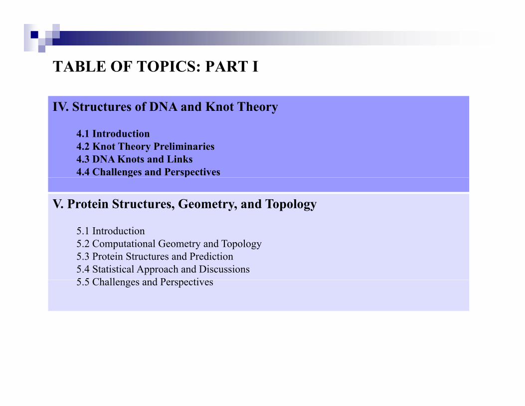
IV. Structures of DNA and Knot Theory
4.1 Introduction4.2 Knot Theory Preliminaries4.3 DNA Knots and Links4.4 Challenges and Perspectivesg p
V. Protein Structures, Geometry, and Topology
5 1 I t d ti5.1 Introduction5.2 Computational Geometry and Topology5.3 Protein Structures and Prediction5.4 Statistical Approach and Discussions5 5 Ch ll d P ti5.5 Challenges and Perspectives
TABLE OF TOPICS: PART II
VI. Biological Networks and Graph Theory
6 1 Introduction6.1 Introduction6.2 Graph Theory and Network Topology6.3 Models of Biological Networks 6.4 Challenges and Perspectives
VII. Biological Systems, Fractals, and Systems Biology
7.1 Introduction 7.2 Fractal Geometry Preliminaries7.3 Fractal Geometry in Biological Systems 7.4 Systems Biology and Perspectives7.5 Challenges and Perspectives
VIII Matrix Genetics Hadamard Matrix and Algebraic BiologyVIII. Matrix Genetics, Hadamard Matrix, and Algebraic Biology
8.1 Introduction8.2 Degeneracy of the Genetic Code 8 3 Th G ti C d d H d d M t i8.3 The Genetic Code and Hadamard Matrices8.4 Genetic Yin-Yang Algebras8.5 Challenges and Perspectives
TABLE OF TOPICS: PART II
IX. Bioinformatics, Living Systems and Cognitive Informatics
9 1 I t d ti9.1 Introduction9.2 Emerging Pattern, Dissipative Structure, and Evolving Cognition9.3 Denotational Mathematics and Cognitive Computing9.4 Challenges and Perspectives
X. The Evolutionary Trends and Central Dogma of Informatics
10.1 Introduction10.1 Introduction10.2 Evolutionary Trends of Information Sciences10.3 Central Dogma of Informatics10.4 Challenges and Perspectives
INTRODUCTION: FUNDAMENTAL QUESTIONS
What is matter? → Physical SciencesWhat is matter? → Physical SciencesWhat is life? → Biological Sciences
What is mind? → New Science of MindWhat is mind? New Science of MindWhat is information? → Informatics
WORDS ON BIOLOGY AND MATHEMATICS…
There's millions and millions of unsolved problems. Biology is so digital,There s millions and millions of unsolved problems. Biology is so digital, and incredibly complicated, but incredibly useful. Biology easily has 500 years of exciting problems to work on, it's at that level.
Don KnuthDon Knuth
Where the telescope ends, the microscope begins. Which of the two has the grander view?grander view?
Victor Hugo
Mathematics if Biology’s Next Microscope, only better; Biology is Mathematics’ Next Physics, Only Better.
Joel Cohen
FROM GENETIC CODE TO LIFEFROM GENETIC CODE TO LIFE
Lif i f d d th ti l tt f th h i l ld G tiLife is founded on mathematical pattern of the physical world. Genetics exploits and organized these patterns. Mathematical regularities are exploited by the organic world at every level of form, structure, pattern, behavior, interaction, and evolution. (Ian Stewart, Life’s other secret), , ( , )
The Natural Technology of genetic coding is major and most effective technology ensuring life on our planet. And acquirement of this technology, occurring in modern time, is major movement in evolution of mankind. The biological evolution can be interpreted as process of deployment and duplicating of the certain forms of ORDERING. (Surgey Petokhov The Biperiodic table of genetic code and number of protons)Petokhov, The Biperiodic table of genetic code and number of protons)
CENTRAL DOGMA OF MOLECULAR BIOLOGY
GeneticsDNA: A, C, G & T (RNA): A, C, G & U
Codons (Triplets)A t i t i i th f th bA string containing three of the abovecharacters
Ex AUG ACU GAC UAA/ UAG /UGAEx. AUG, ACU, GAC, UAA/ UAG /UGA …
Symmetrical Analysis Techniques for Genetic Systems and Bioinformatics: Advanced Patterns and Applications (Sergey Petoukhov and Matthew He IGI Global 2009)Petoukhov and Matthew He, IGI Global, 2009)
Mathematics of Bioinformatics: Theory, Practice, and y, ,Applications (Matthew He and Sergey Petoukhov, in press, Wiley-Interscience, 2011)
Part I Genetic Codes Biological Sequences DNAPart I Genetic Codes, Biological Sequences, DNA and Protein Structures
1. Bioinformatics and Mathematics
IntroductionGenetic Code and MathematicsMathematical BackgroundgConverting Data to KnowledgeBig Picture: InformaticsChallenges and PerspectivesChallenges and Perspectives
1.1 INTRODUCTION
Mathematics and biological data have a synergistic relationship:
Biological information creates interesting problems.Mathematical theory and methods provides models to understand them.Biology validates the mathematical models.
A model is a representation of a real system.A model is a representation of a real system.
Real systems are too complicated, and observation may change the real system. A good system model should be simple, yet powerful enough to capture the behaviors of the real system. Models are especially useful in bioinformatics. p y
Historical Background
Mendel’s genetic experiments and laws of heredity: The discovery of i i h i b G M d l b k i 1865 id d hgenetic inheritance by Gregory Mendel back in 1865 was considered as the
start of bioinformatics history.
The Law of SegregationThe Law of SegregationThe Law of Independent AssortmentThe Law of Dominance
Origin of species: Charles Darwin published “On the Origin of Species” by Means of Natural Selection (Darwin, 1859) or The Preservation of Favored Races in the Struggle for Life" in 1895.
First genetic map: In 1910, after the rediscovery of Mendel’s work, Thomas Hunt Morgan did crossing experiments with the fruit fly (Drosophila Melanogaster) at Columbia University He proved that the(Drosophila Melanogaster) at Columbia University. He proved that the genes responsible for the appearance of a specific phenotype were located on chromosomes.
Historical Background
Transposable genetic elements: In 1944 Barbara McClintock discovered that genes can move on a chromosome. Genes can jump from one chromosome to another.
DNA double helix: In 1953, James Watson and Francis Crick proposed a double helix model of DNA. They suggested that genetic information flows only in one direction, from DNA to messenger RNA to protein, the central concept of the central dogma.
Genetic code: The genetic code was finally "cracked" in 1966. Marshall Ni b H i i h M th i d S O h d t t d th tNirenberg, Heinrich Mathaei and Severo Ochoa demonstrated that a sequence of three nucleotide bases, a codon or triplet, determines each of the 20 amino acids found in nature.
Historical Background
First recombinant DNA molecules: In 1972, Paul Berg of Stanford University (USA) created the first recombinant DNA molecules by combining the DNA of two different organisms.
DNA i d d t b I l 1974 F d i k S f thDNA sequencing and database: In early 1974, Frederick Sanger from the U.K. Medical Research Council was first to invent DNA sequencing techniques. During his experiments to uncover the amino acids in bovine insulin he developed the basics of modern sequencing methodsinsulin, he developed the basics of modern sequencing methods.
Human Genome Project: In 1990, the U.S. Human Genome Project started as a 15-year effort coordinated by the U.S. Department of Energy y y p gyand the National Institutes of Health. The project originally was planned to last 15 years, but rapid technological advances accelerated the expected completion date to 2003.
Historical Background
HG Project goals were to:
identify all the genes in human DNA,determine the sequences of the 3 billion chemical base pairs that makedetermine the sequences of the 3 billion chemical base pairs that make up human DNA, store this information in databases, improve tools for data analysis,transfer related technologies to the private sector andtransfer related technologies to the private sector, andaddress the ethical, legal, and social issues that may arise from the project.
The draft human genome sequence was published on February 15th 2001, in the journals Nature and Science.
1.2 GENETIC CODE AND MATHEMATICS
The secrets of life are more complex than DNA and the genetic code:
One secret of life is the self-assembly of the first cell with a genetic blueprint that allowed it to grow and divide. p g
Another secret of life may be the mathematical control of life as we know it and the logical organization of the genetic code and the use of math in understanding life.
All knowledge is intrinsically unified and lies in a small number of natural la slaws.
1.2 GENETIC CODE AND MATHEMATICS
Math can be used to understand life from the molecular to the biosphere level
the origin and evolution of organisms, the nature of the genomic blueprintsthe universal genetic code ecological relationships.g p
Math helps us look for trends, patterns and relationships that may or may not be obvious to scientists.not be obvious to scientists.
Math allows us to describe the dimensions of genes, sizes of organelles, cells organs and whole organismscells, organs and whole organisms.
1.3 MATHEMATICAL BACKGROUND
ALGEBRA: Algebra is the study of structure, relation and quantity through symbolic operations for the systematic solution of equations and inequalities. In addition to working directly with numbers, algebra works with symbols, variables, and set elements.
ABSTRACT ALGEBRA: Abstract algebra extends the familiar concepts from basic algebra to more general concepts. Abstract algebra deals with the more general concept of sets: a collection of all objects selected bythe more general concept of sets: a collection of all objects selected by property, specific for the set under binary operations. Binary operations are the keystone of algebraic structures studied in abstract algebra: they form part of groups, rings, fields and more.part of groups, rings, fields and more.
1.3 MATHEMATICAL BACKGROUND
PROBABILITY: Probability is the language of uncertainty. It is the likelihood or chance that something is the case or will happen. Probability theory is used extensively in areas such as statistics, mathematics, science, philosophy, psychology, and in the financial markets to draw conclusions b h lik lih d f i l d h d l i h i fabout the likelihood of potential events and the underlying mechanics of
complex systems. An impossible event has a probability of 0, and a certain event has a probability of 1.
STATISTICS: Statistics is a mathematical science pertaining to the collection, analysis, interpretation or explanation, and presentation of data. Probability and statistics have been successfully used to investigateProbability and statistics have been successfully used to investigate sequence analysis, alignments, profile searches and phylogenetic trees and many problems in bioinformatics.
1.3 MATHEMATICAL BACKGROUND
DIFFERENTIAL GEOMETRY: Differential geometry is a mathematical discipline that uses the methods of differential and integral calculus to study problems in geometry. In biological and medical sciences, differential geometry has been used to study protein confirmation and l i i f i id bj h h h d h felasticity of non-rigid objects such as human hearts and human faces.
TOPOLOGY: Topology is the mathematical study of the properties that are preserved through deformations twistings and stretchings of objectsare preserved through deformations, twistings, and stretchings of objects. DNA topology and protein topology are active research areas.
KNOT THEORY: Knot theory is the mathematical branch of topology y p gythat studies mathematical knots, which are defined as embeddings of a circle in 3-dimensional Euclidean space, R3. Chemists and biologists use knot theory to understand, for example, chirality of molecules and the actions of enzymes on DNA.
1.3 MATHEMATICAL BACKGROUND
GRAPH THEORY: Graph theory is the study of graphs. Graphs are mathematical structures used to model pairwise relations between objects from a certain collection. Many applications of graph theory exist in the form of network analysis.
FRACTALS: A fractal is generally "a rough or fragmented geometric shape that can be split into parts, each of which is (at least approximately) a reduced-size copy of the whole," a property called self-similarity. Because they appear similar at all levels of magnification, fractals are often considered to be infinitely complex (in informal terms). Approximate f l il f d i Th bj di l lf i ilfractals are easily found in nature. These objects display self-similar structure over an extended, but finite, scale range. Examples include clouds, snow flakes, crystals, mountain ranges, lightning, river networks, cauliflower or broccoli and systems of blood vessels and pulmonarycauliflower or broccoli, and systems of blood vessels and pulmonary vessels.
1.4 CONVERTING DATA TO KNOWLEDGE
The biological information we gain allows us to learn
About ourselves, About our origins, About our place in the world.
The process of converting data to knowledge:
D t Aggregations KnowledgeDataObservation Filters
AggregationsAndIntegrations
AnalysisKnowledgeDiscovery
1.5 BIG PICTURES: INFORMATICS
Structure, behaviors, and interactions of natural and artificial computational systems
Representation, processing, and communication of information in natural and artificial systems
Computational, cognitive and social aspectsp , g p
The central notion is the transformation of information-whether by computation or communication whether by organisms or artifactscomputation or communication, whether by organisms or artifacts.
COMPUTATIONAL SYSTEMS
Natural ArtificialInternal structure, behavior, and interaction with the environment. Construct (or reconstruct) computational systemsConstruct (or reconstruct) computational systemsAnalytical, experimental and engineering methodologies
h l d h i i f i h i dThe computer language systems and their interfaces with various data types are illustrated below.
COMPUTATIONAL SYSTEMS
Communications Between Computer Languages and Data Types
Computer Languages Design Goals
FORTRAN Numerical analysis
LISP Symbolic computation
C System programming
C++ Objects speed compatibilityC++ Objects, speed, compatibilitywith C
Java Objects, internet
l d i i iPerl System administration
Python General programming
1.6 CHALLENGES AND PERSPECTIVES
Integration: How do we incorporate variation among individual units in nonlinear systems and biological systems?
Scaling: How do we explain the interactions among phenomena that occur on a wide range of scales and molecular levels, of space, time, and organizational complexity? g p y
Pattern Discovery: What is the relation between pattern and process both in mathematical and biological systems?mathematical and biological systems?
Part I Genetic Codes Biological Sequences DNAPart I Genetic Codes, Biological Sequences, DNA and Protein Structures
2. Genetic Codes, Matrices, and Symmetrical Techniques2. Genetic Codes, Matrices, and Symmetrical Techniques
IntroductionM t i Th d S t P li i iMatrix Theory and Symmetry PreliminariesGenetic Codes and MatricesChallenges and Perspectives
2.1 INTRODUCTION
All living organisms are unified by nature. All of them have identical molecular bases of the system of genetic codingmolecular bases of the system of genetic coding.
The set of four letters (A, C, G, T/U) forms the complementary pairs C-G and A-U (or A-T).U ( )
The complementary letters C and G are connected by three hydrogen bonds.
The complementary letters A and U (or A and T) are connected by two hydrogen bonds.
The genetic code is named “the degeneracy code” because its 64 encode 20 amino acids and different amino acids are encoded by different quantities of tripletsof triplets.
2.2 MATRIX THEORY AND SYMMETRY PRELIMINARIES
MatrixMatrix
A rectangular table of elements (or entries), which may be numbers or, more generally any abstract quantities that can be added and multipliedmore generally, any abstract quantities that can be added and multiplied.
Matrices are used to describe linear equations, keep track of the coefficients f li t f ti d t d d t th t d d lti lof linear transformations and to record data that depend on multiple
parameters.
Matrix Operations
2.2 MATRIX THEORY AND SYMMETRY PRELIMINARIES
Operation Definition
AdditionGiven m-by-n matrices A and B, their sum A+B is calculated entrywise,
i.e.
(A + B)i j = Ai j + Bi j where 1 ≤ i ≤ m and 1 ≤ j ≤ n(A + B)i,j Ai,j + Bi,j, where 1 ≤ i ≤ m and 1 ≤ j ≤ n.
Scalar multiplication
Given a matrix A and a number (also called a scalar in the parlance of abstract algebra) c, the scalar multiplication cA is given by multiplying every entry of A by c:
( A) A(cA)i,j = c · Ai,j.
Transpose
The transpose of an m-by-n matrix A is the n-by-m matrix AT (also denoted by Atr or tA) formed by turning rows into columns and columns into rows:
(AT)i,j = Aj,i.
Kronecker (or tensor)
Given m-by-m matrix A=(aij) and n-by-n matrix B=(bij), their Kronecker multiplication is mn-by-mn matrix A B:
A B = [a B a B a Btensor) multiplication
A B = [a11B a12B a1mB……………………………a1mB a2mB ammB]
2.2 MATRIX THEORY AND SYMMETRY PRELIMINARIES
SymmetrySymmetryAn object is symmetric with respect to a given mathematical operation, if, when applied to the object, this operation does not change the object or its appearance.appearance.
In 2D geometry the main kinds of symmetry of interest are with respect to the basic Euclidean plane isometries: translations, rotations, reflections, and glide reflections.
Many structural features of molecules are governed by consideration of tsymmetry.
Symmetries may also be found in living organisms including humans and other animalsother animals.
2.3 GENETIC CODE AND MATRIСES
A, C, G, T
STANDARD GENETIC CODE (64! ARRANGEMENTS)
CCC CCA CAC CAA ACC ACA AAC AAACCU CCG CAU CAG ACU ACG AAU AAGCUC CUA CGC CGA AUC AUA AGC AGACUU CUG CGU CGG AUU AUG AGU AGG
UCC UCA UAC UAA GCC GCA GAC GAAUCU UCG UAU UAG GCU GCG GAU GAGUUC UUA UGC UGA GUC GUA GGC GGAUUU UUG UGU UGG GUU GUG GGU GGG
First kind of equivalence: Two pairs of equivalent letters, where A = Cand U = G, are formed according to an attribute, A and C have a propertyand U G, are formed according to an attribute, A and C have a propertyof amino-mutating of two nitrogenous bases – A and C - in RNA underaction of nitrous acid HNO2. The other two bases U and G do not havethe property of amino-mutating and do not have such a located amino-group; so they are equivalent from viewpoint of absence of this attribute.This was classified by Wittmann in 1961. Here we have G = U and A =C.Second kind of equivalence: Second kind of pairs of equivalent letters isformed on the basis of the attribute of complementation of thesenitrogenous bases in molecules of nucleic acids: C = G (they formcomplementary pair with three hydrogen bonds between them) and А =U (they form complementary pair not with three, but with twohydrogen bonds). This equivalence relation is denoted by C = G and A=U.
ATTRIBUTIVE MAPPINGSATTRIBUTIVE MAPPINGS
We’ll use these attributes equivalence to assign RNA bases A, C, G, U values of 0, 1, 2, and 3 for each pair of equivalence The following listsvalues of 0, 1, 2, and 3 for each pair of equivalence. The following lists these assignments:
Case 1: G = U = 0, A = C = 1, amino- mutating absence/present (0, 1)-bi ticombination,
Case 2: C = U = 1, A = G = 2, pyrimidines /purines ring-based (1, 2)-combination,,
Case 3: A = U = 2, C = G = 3, hydrogen bonds-based (2,3)-combination.
ATTRIBUTIVE MAPPINGSATTRIBUTIVE MAPPINGS
Based on these three attributes equivalences and assignments, threemapping relations from R = A C G U to N = 0 1 2 3 weremapping relations from R = A, C, G, U to N = 0, 1, 2, 3 weredefined as follows (onto and subjective):
α: A, C, G, U → 0, 1 with α (G) = α (U) = 0, α(A) = α (C) =1, , C, G, U , (G) (U) , ( ) (C) ,
β: A, C, G, U → 1, 2 with β (C) = β (U) = 1, β (A) = β (G) = 2,
γ: A, C, G, U → 2, 3 with γ (A) = γ (U) = 2, γ (C) = γ (G) = 3.
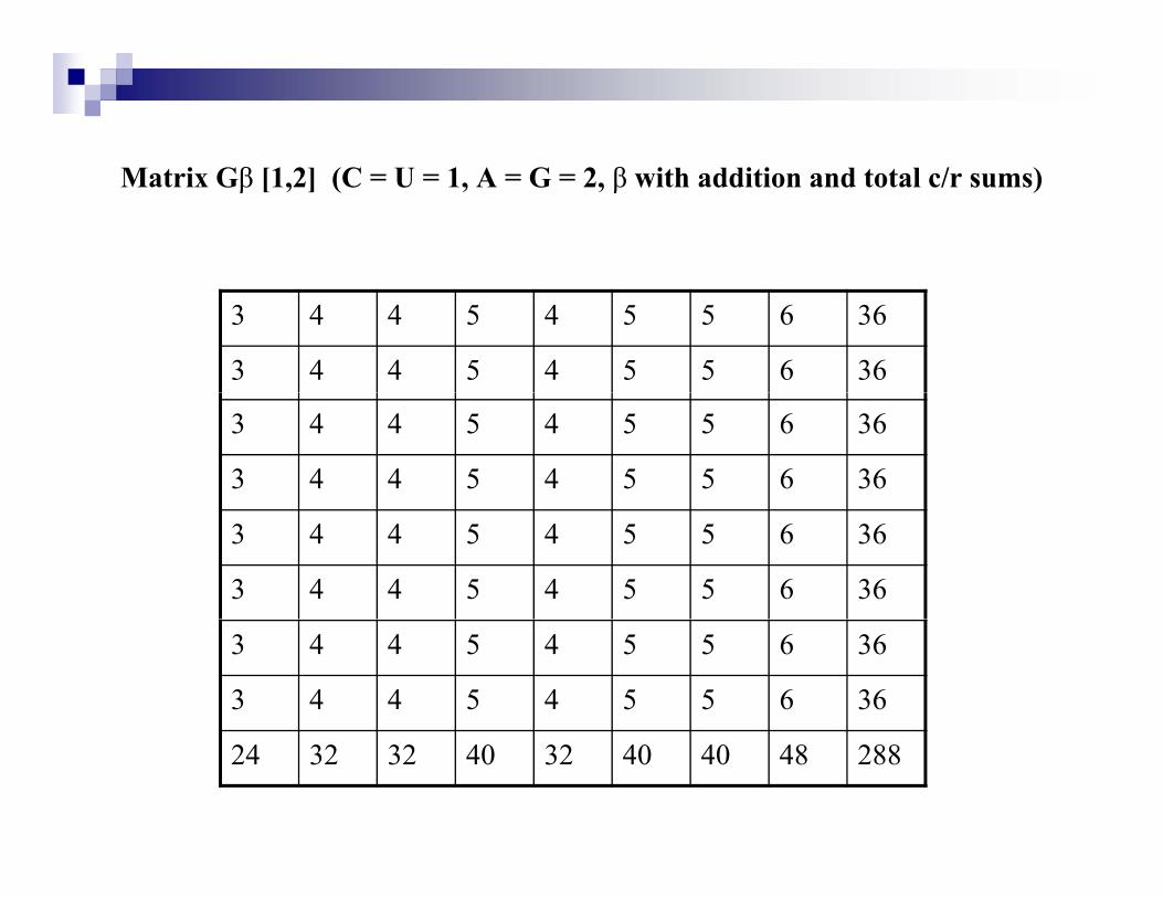
Matrix Gβ [1,2] (C = U = 1, A = G = 2, β with addition and total c/r sums)
3 4 4 5 4 5 5 6 36
3 4 4 5 4 5 5 6 36
3 4 4 5 4 5 5 6 36
3 4 4 5 4 5 5 6 36
3 4 4 5 4 5 5 6 36
3 4 4 5 4 5 5 6 36
3 4 4 5 4 5 5 6 36
3 4 4 5 4 5 5 6 36
24 32 32 40 32 40 40 48 288
Matrix Gγ [2,3] (A = U = 2, C = G = 3, γ with addition and total c/r sums)γ [ , ] ( , , γ )
Basic properties of G [2 3]Basic properties of Gγ [2,3]
These 8 vectors are linearly independent. They form a basis for a vector space of dimension of 8.The power of matrix is stochastic and the limit is a stochastic matrix withThe power of matrix is stochastic and the limit is a stochastic matrix with constant entries.Gγ[2,3]=9P1+8(P2+P3+P4)+7(P5+P6+P7)+6P8
These 8 vectors are linearly independent They form a basis for a vectorThese 8 vectors are linearly independent. They form a basis for a vector space of dimension of 8.The power of matrix is stochastic and the limit is a stochastic matrix with constant entriesconstant entries.Gγ[2,3]=9P1+8(P2+P3+P4)+7(P5+P6+P7)+6P8
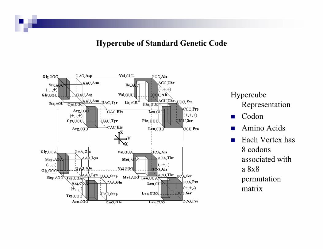
Hypercube of Standard Genetic Codeyp
Hypercube RepresentationCodonAmino AcidsEach Vertex hasEach Vertex has 8 codons associated with a 8x8 a 8 8permutation matrix
2.4 CHALLENGES AND PERSPECTIVES
Why the genetic alphabet consists of four letters?
Why does the genetic code encode 20 amino acids?
H i th t t t f th l l ti d t d ithHow is the system structure of the molecular genetic code connected with known principles of quantum mechanics, which were developed to explain phenomena on atomic and molecular levels?
Why has nature chosen the special code conformity between 64 genetic triplets and 20 amino acids?
What kind of mathematical approach should be chosen among many possible approaches to represent and model structuralized ensembles of molecules of the genetic code?
Part I Genetic Codes Biological Sequences DNAPart I Genetic Codes, Biological Sequences, DNA and Protein Structures
3. Biological Sequences, Sequence Alignment, and Statistics
IntroductionMathematical SequencesSequence AlignmentSequence AlignmentSequence Analysis and Further DiscussionsChallenges and Perspectives
3 1 INTRODUCTION3.1 INTRODUCTION
Biological sequences
DNA sequences (also called genetic sequences or nucleotide sequences). A succession of letters representing the primary structure of a real or hypothetical DNA molecule or strand with the capacity to carryhypothetical DNA molecule or strand, with the capacity to carry information. The possible letters are A, C, G, and T, representing the four nucleotide subunits of a DNA strand - adenine, cytosine, guanine, thymine bases covalently linked to a phospho-backbone. In the typical case, thebases covalently linked to a phospho backbone. In the typical case, the sequences are printed abutting one another without gaps, as in the sequence AAAGTCTGAC, going from 5' to 3' from left to right. DNA sequences instruct the formation of amino acid sequences and N seque ces s uc e o a o o a o ac d seque ces a ddetermine the expression and regulation of genes. They determine the main aspects of the life process.
3 1 INTRODUCTION3.1 INTRODUCTION
Biological sequences
Amino acid sequences (also called peptide sequences or protein sequences).
Amino Acid Alphabets: A, R, …V
Amino acid sequences determine the structures and functions of proteins. The abundant biological sequence data provide us with the most important information of life.
STANDARD AMINO ACID ABBREVIATIONSSTANDARD AMINO ACID ABBREVIATIONS
Amino Acid 3-LetterAbbreviation
1-LetterAbbreviation Amino Acid 3-Letter
Abbreviation1-LetterAbbreviation
Al i Al A L i L LAlanine Ala A Leucine Leu L
Arginine Arg R Lysine Lys K
Asparagine Asn N Methionine Met M
Aspartic acid Asp D Phenylalanine Phe F
Cysteine Cys C Proline Pro P
Glutamic acid Glu E Serine Ser SGlutamic acid Glu E Serine Ser S
Glutamine Gln Q Threonine Thr T
Glycine Gly G Tryptophan Trp W
Histidine His H Tyrosine Tyr Y
Isoleucine Ile I Valine Val V
3.2 MATHEMATICAL SEQUENCES
Mathematical Sequence
An ordered list of objects (or events). It contains members (also called elements or terms).
The number of members (possibly infinite) is called the length of the sequence.
Unlike a set, order matters, and the exact same elements can appear multiple times at different positions in the sequence.
3.2 MATHEMATICAL SEQUENCES
In the language of manoids, a finite set is called an alphabet denoted by Σ. For example,For example,
Σ = 0, 1 is an alphabet of binary numbers: Binary sequencesΣ A C G T i l h b t f DNA b i ti DNAΣ = A, C, G, T is an alphabet of DNA basis. genetic or DNA sequences are sequences over the alphabet of nucleotidesAmino acid sequences are sequences over the alphabet of amino acids
A subsequence of a given sequence is a sequence formed from the given sequence by deleting some of the elements without disturbing the relative positions of the remaining elements.
3.2 MATHEMATICAL SEQUENCES
An infinite binary sequence can represent a formal language (a set of strings) by setting the n-th bit of the sequence to 1 if and only if the nthstrings) by setting the n th bit of the sequence to 1 if and only if the nth string is in the language. Therefore, the study of complexity classes, which are sets of languages, may be regarded as the study of sets of infinite sequences.
An infinite sequence drawn from the alphabet 0, 1, ..., b−1 may also represent a real number expressed in the base-b positional number system.represent a real number expressed in the base b positional number system. This equivalence is often used to bring the techniques of real analysis to bear on complexity classes.
3.3. SEQUENCE ALIGNMENT
The foundation of sequence alignment and analysis is based on the fact that biological sequences develop from pre-existing sequences instead of beingbiological sequences develop from pre existing sequences instead of being invented by nature from the beginning.
The sequence of a gene can be altered in a number of ways Three kinds ofThe sequence of a gene can be altered in a number of ways. Three kinds of changes can occur at any given position within a sequence:
P i t t ti ft d b h i l lf ti f DNAPoint mutations, often caused by chemicals or malfunction of DNA replication, exchange of a single nucleotide for another. Most common is the transition that exchanges a purine for a purine (A ↔ G) or a pyrimidine for a pyrimidine (C ↔ T)pyrimidine for a pyrimidine, (C ↔ T).
3.3. SEQUENCE ALIGNMENT
Insertions add one or more extra nucleotides into the DNA. They are usually caused by transposable elements or errors duringare usually caused by transposable elements or errors during replication of repeating elements (e.g., AT repeats). Insertions in the coding region of a gene may alter splicing of the mRNA (splice site mutation), or cause a shift in the reading frame (frame shift), both of which can significantly alter the gene product. Insertions can be reverted by excision of the transposable element.
Deletions remove one or more nucleotides from the DNA. Like insertions, these mutations can alter the reading frame of the gene. Note that a deletion is not the exact opposite of an insertion: the former is quite random while the latter consists of a specific sequence inserting at locations that are not entirely random or even quite narrowly defined.
3.3 SEQUENCE ALIGNMENT
An alignment between two (or more) sequences is a pairwise (multiple) comparison between the characters of each sequencecomparison between the characters of each sequence
The basic sequence analysis is to ask if two or more sequences are related.
A true alignment of biological sequences is one that reflects the evolutionary relationship between two or more homology which are the
th t h tsequences that share a common ancestor.
3.3 SEQUENCE ALIGNMENT
The key issues to sequence alignments are
What sorts of alignment should be considered:The scoring system used to rank alignments;The algorithm used to find optimal (or good) scoring alignments;The statistical methods used to evaluate the significance of an alignment score.
Biological sequence alignment is a difficult problem (The Number of Alignments!)
THE NUMBER OF ALIGNMENTS
Let a = a1 a2 . . . am and b = b1 b2 . . . bn be two sequences over the alphabet Σ of length, n and m. An alignment of the sequences a and b is a pair ofΣ of length, n and m. An alignment of the sequences a and b is a pair of sequences a* = a a … a and b* = b b … b of equal length of L defined by inserting blanks to the sequences a and b over the extended alphabet Σ *= Σ -. The alignment of a* and b* is represented in a tabular form:
a1 a2 . . . am
b b bb1 b2 . . . bnwhere maxm, n ≤ L ≤ m + n. When L= m + n, the alignment is given by
a1 a2 . . . am - - …. -- - … - b1 b2 . . . bn
THE NUMBER OF ALIGNMENTS
A column that contains two identical characters is called a match, A column that contains two different nonblank characters is called mismatchmismatch, A column that contains a blank is called an indel (insertion/deletion).
The total number of alignments f(m, n) satisfies following recurrence relation:
)1,()1,1(),1(),( −+−−+−= nmfnmfnmfnmfThis recurrence relation was derived by Waterman and it was demonstrated that this number increases rapidly. For example, two sequences of length 1000 have
alignments....4.76710)1000,1000( ≈f
PAIRWISE SEQUENCE ALIGNMENT
Pairwise sequence alignment methods are used to find the best-matching i i (l l) l b l li fpiecewise (local) or global alignments of two query sequences.
Pairwise alignments can only be used between two sequences at a time, but they are efficient to calculate and are often used for methods that do notthey are efficient to calculate and are often used for methods that do not require extreme precision (such as searching a database for sequences with high homology to a query).
Three primary methods of producing pairwise alignments are Global alignment, Local alignmentLocal alignment,Global-local alignment.
GLOBAL ALIGNMENT
Global alignments, which attempt to align every residue in every sequence, f l h h i h i il d fare most useful when the sequences in the query set are similar and of
roughly equal size.
It provides the common means to measure the degree of overall similarity between two sequences. FASTA (FAST ALL) developed by Pearson and Lipman (Pearson and Lipman, 1988) is a heuristic algorithm for global
li I ’ id l d li i llsequence alignment. It’s widely used to align a query sequence against all sequences of a database.
GLOBAL ALIGNMENT
Here is a commonly used algorithm for optimal global alignment. We point h h i l li d d h i d hout that the optimal alignments depend on the input sequences and the
algorithm parameters. The algorithm parameters assigned to matches, mismatches and indels are determined by experience.
Optimal sequence alignment is closely related to the problem of finding the optimal edit distance in binary code. This is an old problem in coding h i d d b L h i (L h i 1966) Th h ftheory introduced by Levenshtein (Levenshtein, 1966). The theory of
semigroups and manoids provides the mathematical background for the manipulation of words over a finite alphabet.
SCORE FUNCTION/SIMILARITY SCORES
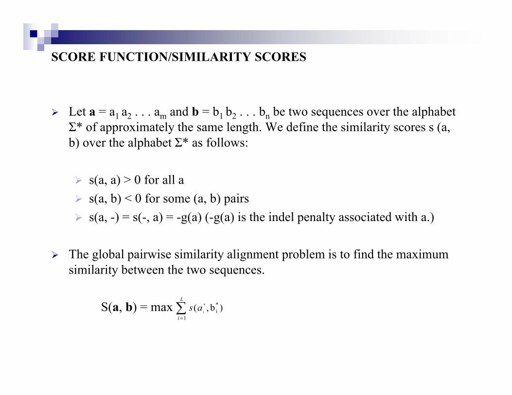
Let a = a1 a2 . . . am and b = b1 b2 . . . bn be two sequences over the alphabet Σ* f i l h l h W d fi h i il i (Σ* of approximately the same length. We define the similarity scores s (a, b) over the alphabet Σ* as follows:
s(a, a) > 0 for all as(a, b) < 0 for some (a, b) pairss(a, -) = s(-, a) = -g(a) (-g(a) is the indel penalty associated with a.)( , ) ( , ) g( ) ( g( ) p y )
The global pairwise similarity alignment problem is to find the maximum similarity between the two sequencessimilarity between the two sequences.
S(a, b) = max ∑=
L
iias
1
*i )b,( *
SCORE FUNCTION/SIMILARITY SCORES
where the maximum is over all alignments. Here the individual score s(x, ) b d fi dy) may be defined as
s (x, y) = log yx
qqp ,
where px,y is the probability of the characters x and y to occur as an aligned column pair in a pairwise alignment of the match model defined as
yxqq
P(a, b| M) = yxp ,∏
And qx is the relative frequency of the character x to occur in the sequences a and b in the random model R defined as
P(a, b| R) = xq∏ yq∏
SCORE FUNCTION/DISTANCE MEASURES
The distance measure can be defined for the global pairwise distance alignment. Let d(a, b) be the distance over the alphabet Σ* as below:
d(a, a) = 0 for all ad(a, b) = d(b, a), cost of a mutation of a into b d( ) d( ) ( ) i i f i id(a, -) = d(-, a) = g(a), positive cost of inserting or deleting of the character a.
DefineD(a, b) = min
where the minimum is over all alignments of a with b
∑=
L
iiad
1
*i )b,( *
where the minimum is over all alignments of a with b.
The main results on global pairwise alignment are stated below.
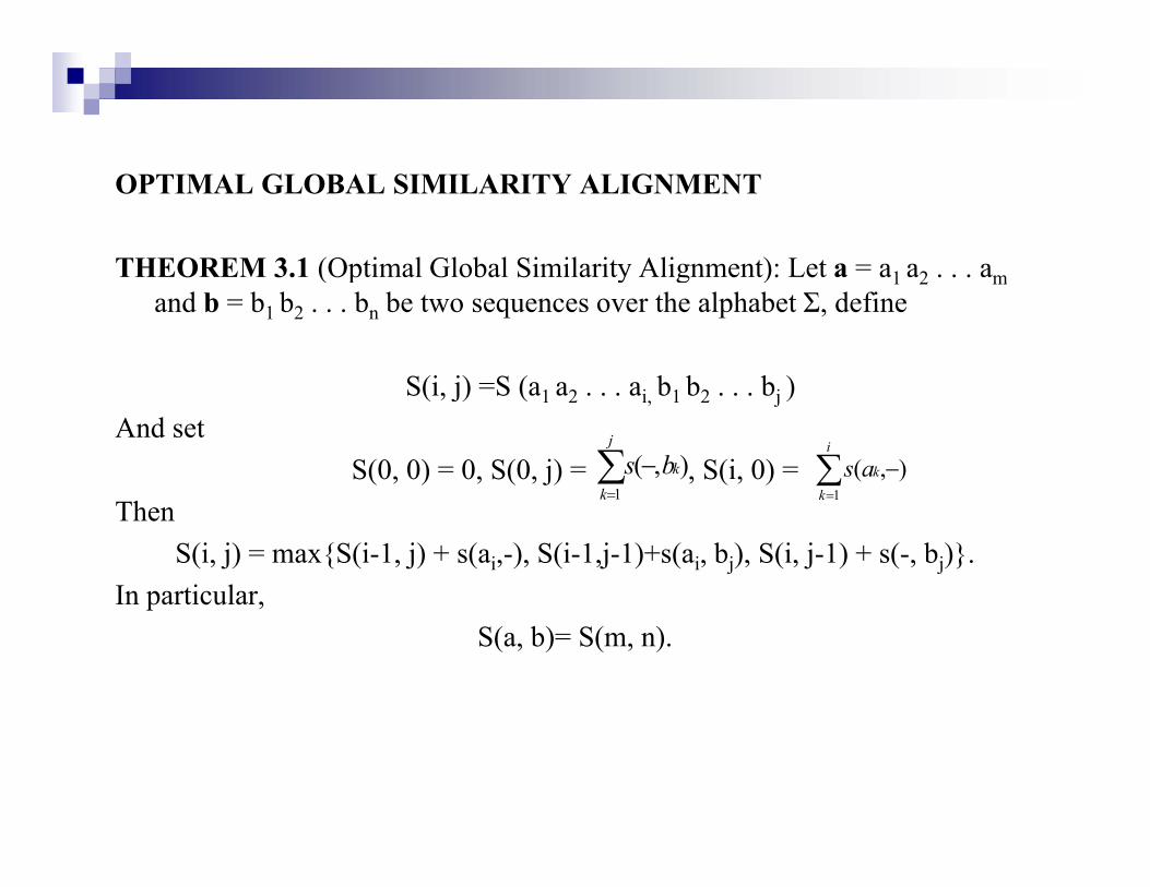
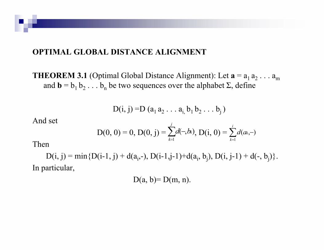
OPTIMAL GLOBAL SIMILARITY ALIGNMENT
THEOREM 3.1 (Optimal Global Similarity Alignment): Let a = a1 a2 . . . amTHEOREM 3.1 (Optimal Global Similarity Alignment): Let a a1 a2 . . . amand b = b1 b2 . . . bn be two sequences over the alphabet Σ, define
S(i j) =S (a a a b b b )S(i, j) =S (a1 a2 . . . ai, b1 b2 . . . bj )And set
THEOREM 3.1 (Optimal Global Distance Alignment): Let a = a1 a2 . . . amTHEOREM 3.1 (Optimal Global Distance Alignment): Let a a1 a2 . . . amand b = b1 b2 . . . bn be two sequences over the alphabet Σ, define
D(i j) =D (a a a b b b )D(i, j) =D (a1 a2 . . . ai, b1 b2 . . . bj )And set
Biological sequences often contain similar subsequences that are preservedBiological sequences often contain similar subsequences that are preserved during the course of evolution.
Local alignments are more useful for dissimilar sequences that are suspected to contain regions of similarity or similar sequence motifs within their larger sequence context.
Th bl f fi di hi hl l t d b f t iThe problem of finding highly related subsequences of two sequences is accomplished by local alignment.
The Smith-Waterman algorithm is a general local alignment method alsoThe Smith Waterman algorithm is a general local alignment method also based on dynamic programming. With sufficiently similar sequences, there is no difference between local and global alignments.
LOCAL ALIGNMENTLOCAL ALIGNMENT
The BLAST (Basic Local Alignment Sequence Tool) is a fast heuristic algorithm for local alignment developed by Altschult et al in 1990algorithm for local alignment developed by Altschult et al., in 1990. BLAST finds regions of similarity. Here we consider only the subsequences of consecutive elements. Any subsequence of a sequence a a a has the form a a a forsubsequence of a sequence a1 a2 . . . am has the form ai ai+1 . . . am+k for some 1≤ i ≤ m and k ≤ m-i. We present the optimal local alignment developed by Smith-Waterman algorithm (Smith and Waterman, 1981). Let a = a1 a2 . . . a and b = b1 b2 . . . b be two sequences over the alphabet Σ.a a1 a2 . . . am and b b1 b2 . . . bn be two sequences over the alphabet Σ.
DefineS(ij, kl) =S (ai . . . aj, bk . . . bl ).
Wh t i th i i il it b t b f d b? Th t iWhat is the maximum similarity between subsequences of a and b? That is, find
L (a b) = max S(ij kl) = S (ai aj bk bl ) | 1 ≤ i ≤ j ≤ m 1 ≤ k ≤ l ≤ nL (a, b) max S(ij, kl) S (ai . . . aj, bk . . . bl ) | 1 ≤ i ≤ j ≤ m, 1 ≤ k ≤ l ≤ n.
OPTIMAL LOCAL ALIGNMENTOPTIMAL LOCAL ALIGNMENT
THEOREM 3.3 (Optimal Local Alignment): Let a = a1 a2 . . . am and b = b1 b2b be two sequences over the alphabet Σ Define. . . bn be two sequences over the alphabet Σ. Define
L(i,0) = 0, 0 ≤ i ≤ m, L(0, j) = 0, 0 ≤ j ≤ n,and
L(i, j) = max 0, L(i-1, j-1)+ s(ai, bj), L(i-1, j)+ s(ai, -), L(i, j-1)+ s(-, bj)| 1≤ i ≤ m, 1≤ j ≤ n,j
where s(x, y) ≥ 0 if x and y match; s(x, y) ≤ 0 if x and y do not match or one of them is a blank.
ThenThenL(j, l) = max 0, S (ai . . . aj, bk . . . bl ) | 1 ≤ i ≤ j ≤ m, 1 ≤ k ≤ l ≤ n.
Each maximal entry L (j*, l*) of the array L corresponds to an optimal local alignment of the sequences a and balignment of the sequences a and b.
GLOBAL LOCAL ALIGNMENTGLOBAL-LOCAL ALIGNMENT
Global-local alignment (hybrid alignment) compares a sequence with the subsequences of another sequencesubsequences of another sequence.
This can be especially useful when the downstream part of one sequence overlaps with the upstream part of the other sequence. In this case, neither p p p q ,global nor local alignment is entirely appropriate: a global alignment would attempt to force the alignment to extend beyond the region of overlap, while a local alignment might not fully cover the region of overlap by Lipman, at el., in 1984.
Let a = a1 a2 . . . am and b = b1 b2 . . . bn be two sequences of different length th l h b t Σ H l t ≤ Th bl i t fi d thover the alphabet Σ. Here we let m ≤ n. The problem is to find the
maximum matching of the shorter sequence with the longer one. That is, find
H( b) S ( b b ) | 1 ≤ k ≤ l ≤ H(a, b) = max S (a, bk . . . bl ) | 1 ≤ k ≤ l ≤ m.
GLOBAL LOCAL ALIGNMENTGLOBAL-LOCAL ALIGNMENT
THEOREM 3.4 (Optimal Global-Local Alignment): Let a = a1 a2 . . . am and b = b b b be two sequences over the alphabet Σ Define= b1 b2 . . . bn be two sequences over the alphabet Σ. Define
H (0, j) = 0, 0 ≤ j ≤ m, H (i, 0) = , 0 ≤ i ≤ n,AndH(i, j) = max H(i-1, j-1)+ s(ai, bj), H(i-1, j)+ s(ai, -), H(i, j-1)+ s(-, bj)|
1≤ i ≤ m, 1≤ j ≤ n,where s(x, y) ≥ 0 if x and y match; s(x, y) ≤ 0 if x and y do not match or one of ( y) y ( y) y
them is a blank.Then
H(i, j) = max S (ai . . . ai bk . . . bj ) | 1 ≤ i ≤ m, 1 ≤ k ≤ j ≤ n.H(i, j) max S (ai . . . ai, bk . . . bj ) | 1 ≤ i ≤ m, 1 ≤ k ≤ j ≤ n.In particular,
H( b) H ( j) | 1 ≤ j ≤ H(a, b) = max H (m, j) | 1 ≤ j ≤ n.
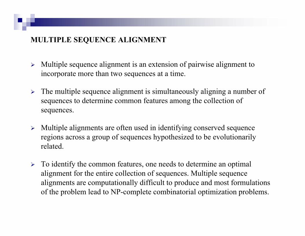
MULTIPLE SEQUENCE ALIGNMENT
Multiple sequence alignment is an extension of pairwise alignment to incorporate more than two sequences at a timeincorporate more than two sequences at a time.
The multiple sequence alignment is simultaneously aligning a number of sequences to determine common features among the collection of q gsequences.
Multiple alignments are often used in identifying conserved sequence regions across a group of sequences hypothesized to be evolutionarily related.
T id tif th f t d t d t i ti lTo identify the common features, one needs to determine an optimal alignment for the entire collection of sequences. Multiple sequence alignments are computationally difficult to produce and most formulations of the problem lead to NP-complete combinatorial optimization problemsof the problem lead to NP-complete combinatorial optimization problems.
MULTIPLE SEQUENCE ALIGNMENT
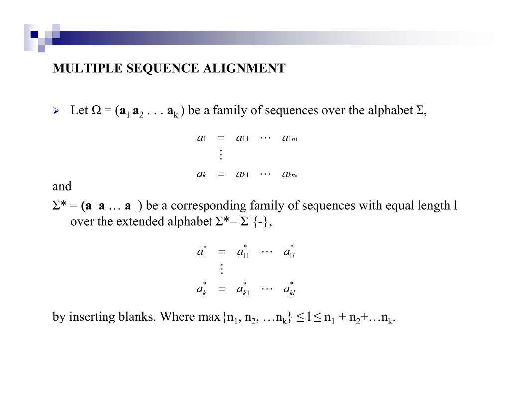
Let Ω = (a1 a2 . . . ak ) be a family of sequences over the alphabet Σ,
kknkk
n
aaa
aaa
L
M
L
1
1111 1
=
=
and Σ* = (a a … a ) be a corresponding family of sequences with equal length l
over the extended alphabet Σ*= Σ -,
kknkk aaa 1
p
*1
*11
*
1 laaaM
L=
by inserting blanks. Where maxn1, n2, …nk ≤ l ≤ n1 + n2+…nk.
**1
*klkk aaa L=
MULTIPLE SEQUENCE ALIGNMENT
The optimal global alignment is to find the maximum similarity between these sequences Ω in terms of a scoring function s (Ω*) that isthese sequences Ω in terms of a scoring function s (Ω*), that is
S(Ω)= max s(Ω*) | Ω* is a multiple alignment of Ω,
where s(Ω*) = ∑
l
ias *ki )a,...,( *
1( )
is the sum of scores of the columns. Here it is assumed that the columns of the alignment are statistically independent. We are now in a position to
∑=i 1
the alignment are statistically independent. We are now in a position to state the optimal multiple sequence alignment result.
OPTIMAL GLOBAL MULTIPLE SEQUENCE ALIGNMENT
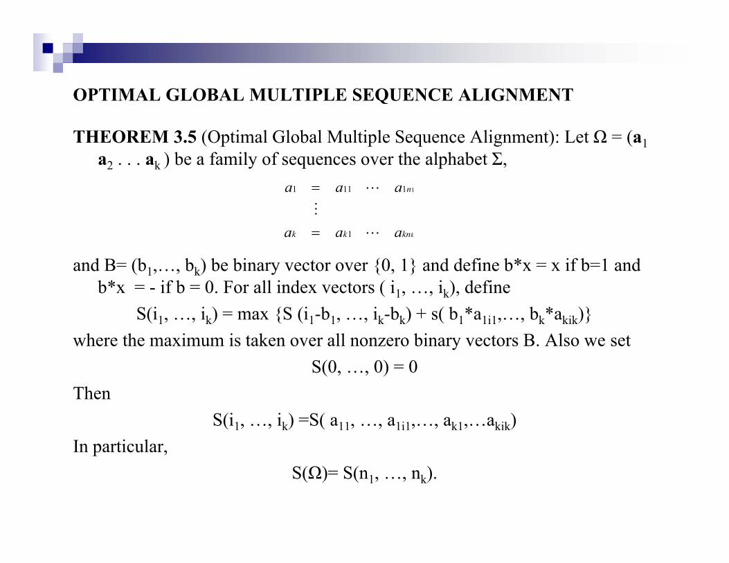
THEOREM 3.5 (Optimal Global Multiple Sequence Alignment): Let Ω = (a1 a2 . . . ak ) be a family of sequences over the alphabet Σ,
kknkk
n
aaa
aaa
L
M
L
1
1111 1
=
=
and B= (b1,…, bk) be binary vector over 0, 1 and define b*x = x if b=1 and b*x = - if b = 0. For all index vectors ( i1, …, ik), define
S(i1 ik) = max S (i1-b1 ik-bk) + s( b1*a1i1 bk*akik)S(i1, …, ik) max S (i1 b1, …, ik bk) + s( b1 a1i1,…, bk akik)where the maximum is taken over all nonzero binary vectors B. Also we set
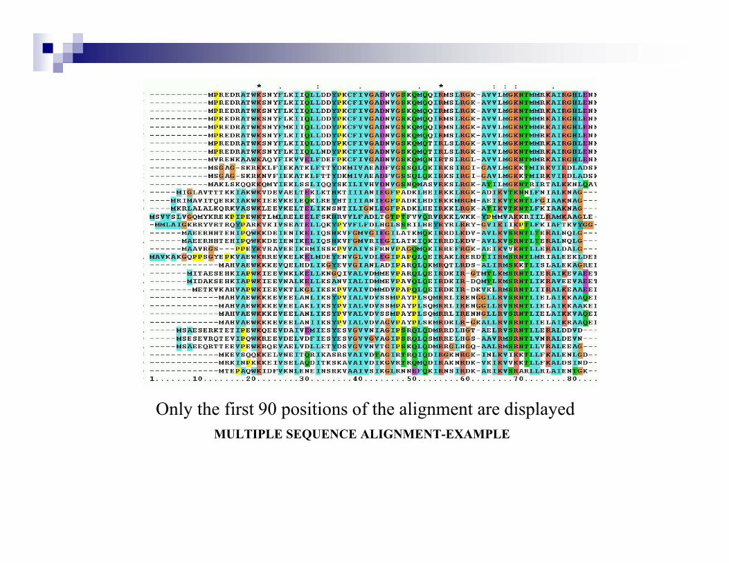
EXAMPLE Here we display the representation of a protein multiple sequence alignment produced with ClustalW (Chenna at el 2003) Thesequence alignment produced with ClustalW (Chenna, at el., 2003). The sequences are instances of the acidic ribosomal protein P0 homolog (L10E) encoded by the Rplp0 gene from multiple organisms. The protein sequences were obtained from SwissProt searching with the gene name.sequences were obtained from SwissProt searching with the gene name. This is generated by Miguel Andrade February 2006 (UTC).
TABLE 3 2 Only the first 90 positions of the alignment are displayed TheTABLE 3.2 Only the first 90 positions of the alignment are displayed. The colours represent the amino acid conservation according to the properties and distribution of amino acid frequencies in each column. Note the two completely conserved residues arginine (R) and lysine (K) marked with ancompletely conserved residues arginine (R) and lysine (K) marked with an asterisk at the top of the alignment.
Only the first 90 positions of the alignment are displayedMULTIPLE SEQUENCE ALIGNMENT-EXAMPLE
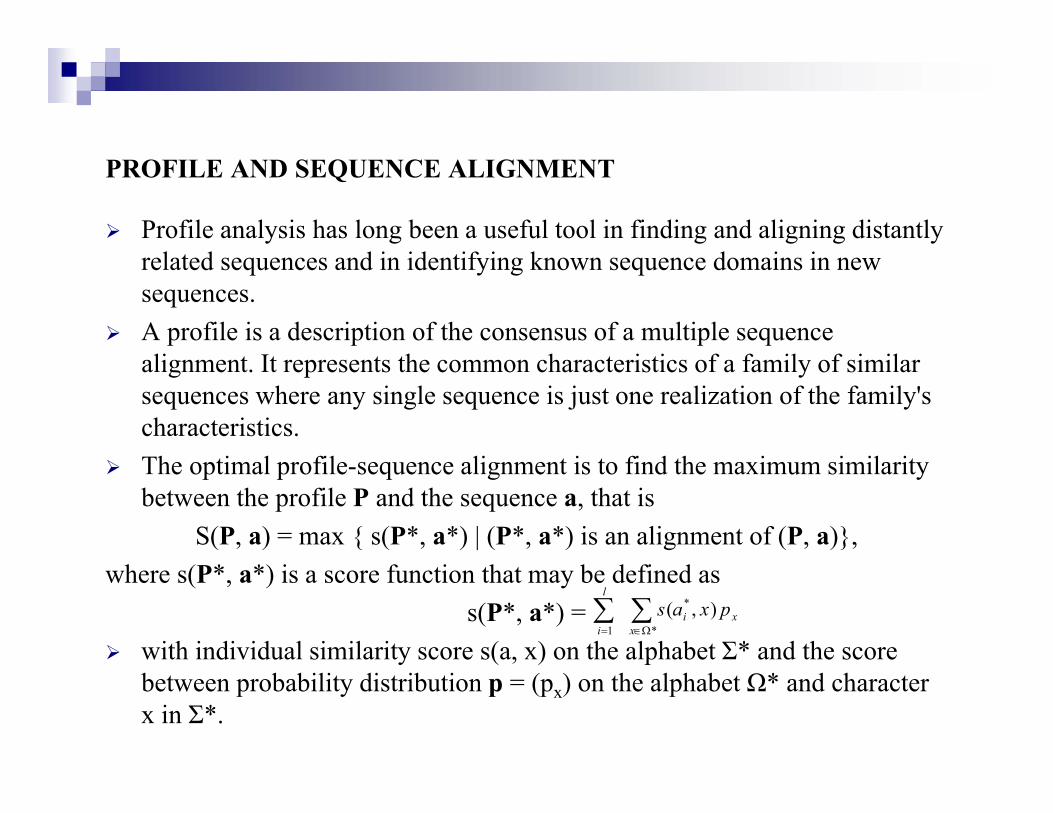
PROFILE AND SEQUENCE ALIGNMENT
Profile analysis has long been a useful tool in finding and aligning distantly l d d i id if i k d i irelated sequences and in identifying known sequence domains in new
sequences. A profile is a description of the consensus of a multiple sequence li I h h i i f f il f i ilalignment. It represents the common characteristics of a family of similar
sequences where any single sequence is just one realization of the family's characteristics.Th i l fil li i fi d h i i il iThe optimal profile-sequence alignment is to find the maximum similarity between the profile P and the sequence a, that is
S(P, a) = max s(P*, a*) | (P*, a*) is an alignment of (P, a),where s(P*, a*) is a score function that may be defined as
s(P*, a*) = with individual similarity score s(a, x) on the alphabet Σ* and the score
xix
l
ipxas ),( *
*1∑∑Ω∈=
y ( , ) pbetween probability distribution p = (px) on the alphabet Ω* and character x in Σ*.
PROFILE AND SEQUENCE ALIGNMENT
Theorem 3.6 (Optimal Profile-Sequence Alignment): Let P = p1 p2 . . . pn be h fil f l i l li d bthe profile of a multiple sequence alignment and a = a1 a2 . . . an be a
sequence over the alphabet Σ*, define
S(i j) S ( ) 1 i 1 jS(i, j) =S (p1 p2 . . . pi, a1 a2 . . . aj ), 1≤ i ≤ m, 1≤ j ≤ nand set
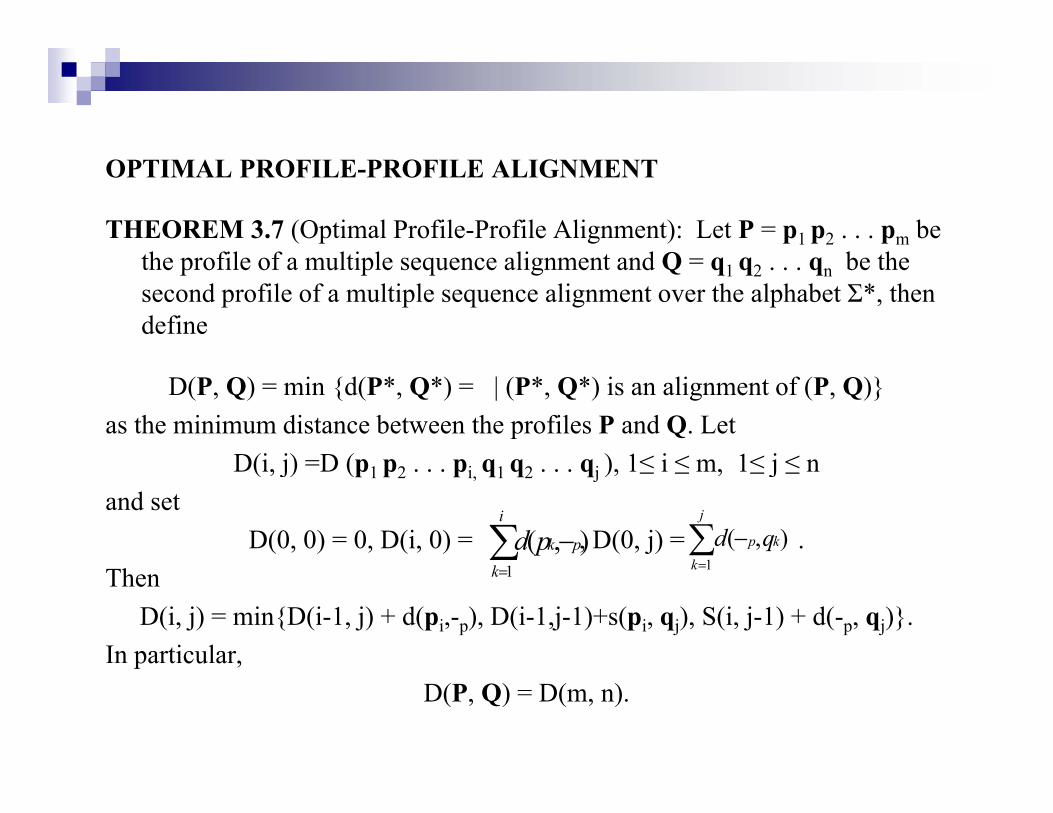
THEOREM 3.7 (Optimal Profile-Profile Alignment): Let P = p1 p2 . . . pm be h fil f l i l li d Q b hthe profile of a multiple sequence alignment and Q = q1 q2 . . . qn be the
second profile of a multiple sequence alignment over the alphabet Σ*, then define
D(P, Q) = min d(P*, Q*) = | (P*, Q*) is an alignment of (P, Q)as the minimum distance between the profiles P and Q. Let
D(i j) D ( ) 1≤ i ≤ 1≤ j ≤D(i, j) =D (p1 p2 . . . pi, q1 q2 . . . qj ), 1≤ i ≤ m, 1≤ j ≤ nand set
A hidden Markov model (HMM) is a statistical model in which the system being modeled is assumed to be a Markov process with unknown parameters, and the challenge is to determine the hidden parameters from the observable parameters. Hidden Markov models are especially known for their application in temporal pattern recognition such as speech, handwriting, gesture
i i i l f ll i i l di h d bi i f irecognition, musical score following, partial discharges and bioinformatics.
Pattern Discovery: Given a sequence of data such as a DNA or amino acid sequence a motif or a pattern is a repeating subsequence Such repeatedsequence, a motif or a pattern is a repeating subsequence. Such repeated subsequences often have important biological significance and hence discovering such motifs in various biological databases turns out to be a very important problem in computational biology. Of course, in biologicalimportant problem in computational biology. Of course, in biological applications the various occurrences of a pattern in the given sequence may not be exact and hence it is important to be able to discover motifs even in the presence of small errors. Various tools are now available for carrying out p y gautomatic pattern discovery. This is usually the first step towards a more sophisticated task such as gene finding in DNA or secondary structure prediction in protein sequences at system level.
Scoring functions: The choice of a scoring function that reflects bi l i l i i l b i b k i ibiological or statistical observations about known sequences is important to producing good alignments.
Structural alignments which are usually specific to protein andStructural alignments, which are usually specific to protein and sometimes RNA sequences, use information about the secondary and tertiary structure of the protein or RNA molecule to aid in aligning the sequences. These methods can be used for two or more sequences andsequences. These methods can be used for two or more sequences and typically produce local alignments; however, because they depend on the availability of structural information, they can only be used for sequences whose corresponding structures are known (usually through X-ray crystallography or NMR spectroscopy).
3.5 CHALLENGES AND PERSPECTIVES3.5 CHALLENGES AND PERSPECTIVES
The issues need to be addressed may include:
Architecture of Data and Knowledge RepositoriesDatabases: Flat, Relational and Object-Oriented; what is most
i t ?appropriate?The imminent need for Ontologies in biologyThe Middle Layer: How to design it?Applications and integration of applications into the middle layerReduction and Analysis of Data: the largest challenge!How to integrate legacy knowledge with data?How to integrate legacy knowledge with data?User Interfaces: web browser and beyond
Part I Genetic Codes Biological Sequences DNAPart I Genetic Codes, Biological Sequences, DNA and Protein Structures
4. Structures of DNA and Knot Theory
IntroductionKnot Theory PreliminariesDNA Knots and LinksDNA Knots and LinksChallenges and Perspectives
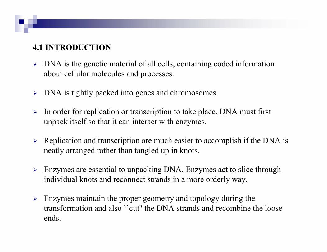
4 1 INTRODUCTION4.1 INTRODUCTION
DNA is the genetic material of all cells, containing coded information about cellular molecules and processes.
DNA is tightly packed into genes and chromosomes.
I d f li ti t i ti t t k l DNA t fi tIn order for replication or transcription to take place, DNA must first unpack itself so that it can interact with enzymes.
Replication and transcription are much easier to accomplish if the DNA isReplication and transcription are much easier to accomplish if the DNA is neatly arranged rather than tangled up in knots.
Enzymes are essential to unpacking DNA. Enzymes act to slice through y p g y gindividual knots and reconnect strands in a more orderly way.
Enzymes maintain the proper geometry and topology during the f i d l `` '' h DNA d d bi h ltransformation and also ``cut'' the DNA strands and recombine the loose
ends.
DNA STRUCTURESDNA STRUCTURES
B-DNA: Fully hydrated DNA, the most common encountered in vivo. Owing to the location of the helical axis in the center of the base pairs, the edges of the base pairs are about equally deep in the interior.
A-DNA: When B-DNA is dehydrated, there is a reversible structural h t A DNAchange to A-DNA
Z-DNA: Unlike B-DNA and A-DNA, Z-DNA is a left-handed helix. The conformational change from B-DNA to Z-DNA is one mechanism forconformational change from B-DNA to Z-DNA is one mechanism for relief of the torsional strain found in B-DNA in vivo, and may serve as a switch mechanism to regulate gene expression.
The three structural variations of these grooves ("A", "B" and "Z" DNA), which differ in the relationship between the bases and the helical axis, offer one mechanism by which reactivity of DNA is modulatedone mechanism by which reactivity of DNA is modulated.
FORMS OF DNA
Supercoiled (or "knotted"): Double stranded circular (or linear) DNA canSupercoiled (or knotted ): Double stranded circular (or linear) DNA can have tertiary or higher order structure. Superhelicity is therefore sometimes referred to as DNA's tertiary structure. Supercoils refer to the DNA structure in which double-stranded circular DNA twists around each other.structure in which double stranded circular DNA twists around each other. Supercoiling can be:
negative (right handed): Supercoils formed by deficit in link are callednegative (right-handed): Supercoils formed by deficit in link are called negative supercoils.
iti (l ft h d d) S il f d b i i li kpositive (left-handed): Supercoils formed by an increase in link are called positive supercoils.
FORMS OF DNA
Relaxed: Circular DNA without any superhelical twist is known as aRelaxed: Circular DNA without any superhelical twist is known as a relaxed molecule. DNA in its relaxed (ideal) state usually assumes the B configuration. In a relaxed double-helical segment of DNA, the two strands twist around the helical axis once every 10.6 base pairs of sequence. Thetwist around the helical axis once every 10.6 base pairs of sequence. The following structures are consistent with the relaxed state:
Linear DNA (either straight or curved)Linear DNA (either straight or curved)
Closed circular DNA, provided its axis lies in a plane or on the surface f hof a sphere
FORMS OF DNA
Supercoiling is vital to two major functionsSupercoiling is vital to two major functions
It helps pack large circular rings of DNA into a small space by making the i hi hl trings highly compact.
It also helps in the unwinding of DNA required for its replication and transcription.
Supercoiled DNA is thus the biological active form. The normal biological p g gfunctioning of DNA occurs only if it is in the proper topological state.
4.2. KNOT THEORY PRELIMINARIES
A knot is a closed continuous curve in space that does not intersect itselfA knot is a closed continuous curve in space that does not intersect itself anywhere.
Wh k t i d f d (i t t h d d b t t i t d) b tWhen a knot is deformed (i.e. stretched, compressed, bent, or twisted), but not cut or torn, all the deformed curves will be considered to be the same as the original closed knotted curve.
The simplest knot of all is the unknotted circle, which we call the unknot or the trivial knot denoted by C. The next simplest knot is called a trefoil knot
knot symbol prime knotKnot projection
knot symbol prime knot
01 unknot
31 trefoil knot
41 figure eight knot
51 Solomon's seal knot
61 stevedore's knot
62 Miller Institute knot
Primary Knots
Crossing Number
The crossing number of a knot K denoted by c(K), is the least number of crossings that occur in any projection of the knot. If a knot is nontrivial, then it has more than one crossing in a projection The figure above calledthen it has more than one crossing in a projection. The figure above called the figure-eight knot has four crossings.
COMPOSITION OF KNOTS
Given two projections of knots and assuming the two projections do notGiven two projections of knots and assuming the two projections do not overlap, one can compose a new knot by deleting a small arc from each knot projection and then connecting the four ending points by two new arcs. The resulting knot is called the composition (or knot sum) of the twoarcs. The resulting knot is called the composition (or knot sum) of the two knots, denoted by K1#K2 (or K1+ K2).
Knot MovesKnot Moves
Reidemeister moves
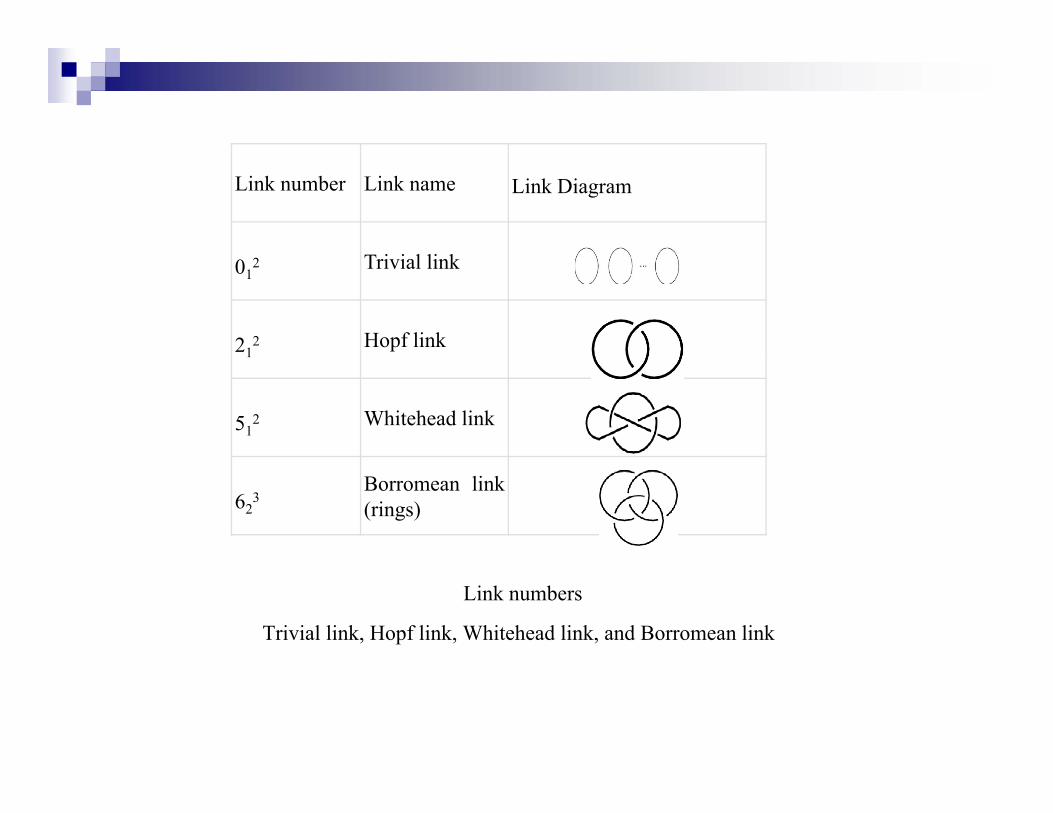
LINKS
A link is the union of a finite number of disjoint knots in three dimensional space.
A knot will be considered a link of one component.
Four common links, known as trivial link (or unlink), the Hopf link, the Whitehead link, and the Borromean links listed in Figure 4.6. The notation and ordering follows that of Rolfsen (1976), where ck
r denotes the kth r-g ( ), kcomponent link with crossing number c.
Two links are considered to be the same if we can deform the one link to the other link without ever having any one of the knots intersect itself or any of the other loops in the process, That is, two links are considered equal if they are isotopic.
Link number Link name Link Diagram
012 Trivial link
212 Hopf link
1
512 Whitehead link
623
Borromean link(rings)
Link numbers
Trivial link, Hopf link, Whitehead link, and Borromean link
LINKING NUMBERLINKING NUMBERFormally, a linking number is defined as the sum of +1 crossings and -1crossing over all crossings between the two links divided by 2 calculated by the following formula:by the following formula:
L(K1, K2) = ,where α ∩ β is the set of crossings of α with β, and ε (p) is the sign of the crossing
21 ∑
∩∈ βα
εp
p )(
crossing. Computing Linking Number:
Let K1 and K2 be two components in a link L, and choose an orientation on h t Th t h i b t th t teach component. Then at each crossing between the two components, we
count a +1 for each crossing of the first type, and a -1 for each crossing of the second type.
COMPUTING LINK NUMBER
In other words, to each of these crossings is associated an index number ofIn other words, to each of these crossings is associated an index number of +1 or -1, according to the direction in which the tangent vector to the top curve must be rotated to coincide with the tangent vector to the bottom curve. If the rotation is clockwise, the index number is -1, and if it is counterclockwise, the index number is +1. Adding all the indices associated to all the crossings and dividing by 2 gives the link number of two knots denoted by L(K1, K2).
PROPERTIES OF LINKING NUMBERS
The linking number L(K1, K2) is a property of the curves in space and isThe linking number L(K1, K2) is a property of the curves in space and is independent of the planar projection.
The linking number L(K1, K2) is unchanged if either of the curves is deformed continuously provided no breaks are made in either curve. Moreover the Reidemeister moves don’t affect linking number.
Th li ki b L(K K ) h i if th di ti f f thThe linking number L(K1, K2) changes sign if the direction of one of the curves is reversed.
The linking number L(K1 K2) changes sign if a pair of curves is reflectedThe linking number L(K1, K2) changes sign if a pair of curves is reflected in a plane.
PROPERTIES OF LINKING NUMBERS
Two oriented curves K1 and K2 bound a ribbon-like surface, the linkingTwo oriented curves K1 and K2 bound a ribbon like surface, the linking number L(K1, K2) is the sum of two geometric quantities: twist T(K1, K2), and writhe W(K1).
L(K1, K2) = T(K1, K2) + W(K1)
Thi i t t h t i ti t th ith th i i f li kiThis important characteristic together with the invariance of linking number have been applied to the study of circular DNA structure by Adams, 1994.
TWIST T(K1, K2)
The twist T(K1, K2) of one curve K1 about another curve K2 measures theThe twist T(K1, K2) of one curve K1 about another curve K2 measures the magnitude of the spinning of K1 around K2. The twist of helices about a linear axis is the number of times the helix (K1) resolves about the axis (K2). This number T(K1, K2) >0 if the helix K1 is right-handed and T(K1, 2 1 2 1 1K2) < 0 if the helix K1 is left-handed (T(K1, K2) =1/2; -1/2; -1)
TWIST T(K1, K2)
For the more general cases in which K2 is not linear, or planar, theFor the more general cases in which K2 is not linear, or planar, the definition of the twist is much more complex for the concept is no longer geometrically obvious. The twist of K1 around K2 is defined to be the measure of the total change of V in the direction of T x V as x moves along the entire curve K2. This is given by the line integral (normalized in turns) over the curve K2:
T(K K ) ∫ )(1 dVVTT(K1, K2) =
This integral is not necessarily an integer. It changes under deformations of
∫ ⋅×2
)(2 K
dVVTπ
either the curve K2 or the corresponding surface. Since the cross-product operation is not commutative, the twist depends on the ordering of the curves. The twist of K1 about K2 is not necessarily the twist of K2 about K1.
WRITHE W(K )WRITHE W(K1)
The writhing number of a curve K1, denoted by W(K1), is a knot property defined as the sum of crossings p of a curve K1,
W(K1) = ∑∈ )( 1
)(KCp
pε
where ε (p) is defined to be ± 1 if the overpass slants from top left to bottom right or bottom left to top right and C(K1) is the set of crossings of an oriented curve
The linking number L(K1, K2) is a topological invariant. However the twist n mber T(K K ) and rithing n mber W(K ) are not and in fact arnumber T(K1, K2) and writhing number W(K2) are not, and in fact, vary under deformation. Therefore, while the twist and a change in writhing could increase or increase linking, the linking number is invariant under deformationdeformation.
4 3 DNA KNOTS AND LINKS4.3. DNA KNOTS AND LINKS
Geneticists have discovered that DNA can form knots and links which can be described mathematically.
By understanding knot theory more completely, scientists are becoming bl t h d th i l it i l d i th lif dmore able to comprehend the massive complexity involved in the life and
reproduction of the cell.
The particular fascination in this process for geneticists is the fact thatThe particular fascination in this process for geneticists is the fact that chemical changes occur in the DNA strand as a result of this process.
Changes in the DNA str ct re d e to the actions of these en mes ha eChanges in the DNA structure due to the actions of these enzymes have required geneticists to use very advanced mathematical topology (which includes knot theory) and geometry in their study of molecular biology.
DESCRIPTIVE PROPERTIES ASSOCIATED WITH SUPERCOILINGDESCRIPTIVE PROPERTIES ASSOCIATED WITH SUPERCOILING
"Supercoiling" is an abstract mathematical property and represents the sum of what are termed "twist" and "writhe". "Supercoil" is the combination of twists and writhes that impart the supercoiling, and these occur in response to a change in the linking number.
Writhing: The writhing number describes the supertwisting or supercoiling of the helix in space. It is the number of turns that the duplex axis makes about the superhelix axis Writhe describes the coiling of the DNA coil Itabout the superhelix axis. Writhe describes the coiling of the DNA coil. It is a measure of the DNA's superhelicity (supercoiling) and can be positive or negative. When a molecule is relaxed and contains no supercoils, the linking number = the twist number since W= 0. The linking number oflinking number the twist number since W 0. The linking number of relaxed DNA is L = N/10.5, where N is the number of base pairs in the DNA fragment.
DESCRIPTIVE PROPERTIES ASSOCIATED WITH SUPERCOILINGDESCRIPTIVE PROPERTIES ASSOCIATED WITH SUPERCOILING
Twisting: Twist is the number of helical turns in the DNA, i.e., the complete revolutions that one polynucleotide strand makes about thecomplete revolutions that one polynucleotide strand makes about the duplex axis in the particular conformation under consideration. Twist is normally the number of base pairs divided by 10.5. Twist is altered by deformation and is a local phenomenon. The total twist is the sum of all ofdeformation and is a local phenomenon. The total twist is the sum of all of the local twists. Twist is a measure of deformation due to a twisting motion.
Linking number: This is a topological property that determines the degree of supercoiling. It defines the number of times a strand of DNA winds in the right-handed direction around the helix axis when the axis is
i d li i l l h i di h h fconstrained to lie in a plane. Topology theory indicates that the sum of T and W equals the linking number: L = T + W. If both strands are covalently intact, the linking number cannot change. Link is thus a topological invariant remaining unaltered even if the two curves are deformed in spaceinvariant, remaining unaltered even if the two curves are deformed in space -- as long as neither is cut.
DESCRIPTIVE PROPERTIES ASSOCIATED WITH SUPERCOILINGDESCRIPTIVE PROPERTIES ASSOCIATED WITH SUPERCOILING
For example, in the circular DNA of 5400 base pairs, the linking number is 5400/10 = 540.
When a molecule is relaxed and contains no supercoils, the linking number th t i t b i W 0 Th if th i ili th W= the twist number since W = 0. Thus if there is no supercoiling, then W =
0, L = T+W= 540.
If there is positive supercoiling W = +20 T = L - W = 520If there is positive supercoiling, W = +20, T = L - W = 520.
4 4 CHALLENGES AND PERSPECTIVES4.4 CHALLENGES AND PERSPECTIVES
In the area of DNA structure, several subareas are particularly amenable to mathematical analysis:
A complete analysis of the packaging of DNA in chromatin. Only the first d ili i t l i d t d B f th l torder coiling into core nucleosomes is understood. By far the largest
compaction of DNA comes from higher order folding.
Presentation of the topological invariants that describe the structure ofPresentation of the topological invariants that describe the structure of DNA and its enzymatic transformations. The goal is to be able to predict the structure of interstate or products from enzymatic mechanisms and in turn to predict mechanisms from structure.p
An analysis of the reciprocal interaction between secondary and higher order structures. This includes the phenomena of bending, looping, and phasing.
4 4 CHALLENGES AND PERSPECTIVES4.4 CHALLENGES AND PERSPECTIVES
Many doubts and suspicions exist in understanding of the genetic language.
How was life information accumulated and evolved in the DNA sequence?
How can we understand the possible function of the large amount of nongenic DNA in the genome and extract life information from DNA sequence under the background of strong noises?
What is the principle that governs the functional networks in a genome?
How can we predict the molecular structure from its sequence information?How can we predict the molecular structure from its sequence information?
Part I Genetic Codes Biological Sequences DNAPart I Genetic Codes, Biological Sequences, DNA and Protein Structures
5. Protein Structures, Geometry, and Topology
I d iIntroductionComputational Geometry and TopologyProtein Structures and PredictionStatistical Approach and DiscussionsChallenges and Perspectives
5.1 INTRODUCTION
Proteins play crucial roles in almost every biological process:
Responsible in one form or another for a variety of physiological functions,
Function as catalysts, y ,
Transport and store other molecules such as oxygen,
P id h i l d i iProvide mechanical support and immune protection,
Generate movement,
Transmit nerve impulses,
Control growth and differentiation.g
5.1 INTRODUCTION
They perform many vital functions e g :They perform many vital functions, e.g.:Catalysis of reactionsTransport of moleculesTransport of moleculesBuilding blocks of musclesStorage of energyDefense against intruders
They are large molecules—containing 100s to 1000s atoms.They are made of amino acids.
There are 20 different types of amino acidsThere are 20 different types of amino acids.
5 2 COPMPUTATIONAL GEOMETRY AND TOPOLOGY5.2 COPMPUTATIONAL GEOMETRY AND TOPOLOGY
C i l GComputational Geometry
The study of efficient algorithms to solve geometric problems, such as given N points in a plane, what is the fastest way to find the nearest neighbor of a point? Given N straight lines, find the lines which intersect with each other.
Many questions in molecular modeling can be understood geometrically in terms of arrangements of spheres in three dimensions.
5.3 COPMPUTATIONAL GEOMETRY AND TOPOLOGY PRELIMINARIES
C i l GComputational Geometry
Problems include computing properties of such arrangements such as their volume and topology, testing intersections and collisions between molecules, finding offset surfaces, data structures for computing inter-atomic forces and performing molecular dynamics simulations, and
hi l i h f d i l l d l lcomputer graphics algorithms for rendering molecular models accurately and efficiently.
Computational geometry can be also used as a tool for studying topology and architecture of macromolecules and macromolecular complexes.
FUNDAMENTAL GEOMETRIC OBJECTS
Polygons: A polygon is a collection of line segments, forming a cycle, and not crossing each other A polygon can be represented as a sequence ofnot crossing each other. A polygon can be represented as a sequence of points.
Convex Hull: The convex hull of a set of points S in n dimensions is the C p Sintersection of all convex sets containing S.
Finding the convex hull of a set of points is the most elementarily interesting problem in computational geometry, just as the minimum spanning tree is the most elementarily interesting problem in graph algorithms.
Novel patterns based on convex hull representation are firstly extracted from a protein structure, then the classification system is constructed and machine learning methods such as neural networks and Hidden Markov Models (HMM) have been applied.
FUNDAMENTAL GEOMETRIC OBJECTS
Triangulation: Triangulation is the division of a surface or plane polygon into a set of triangles, usually with the restriction that each triangle side is
i l h d b dj i lentirely shared by two adjacent triangles.
Triangulation is a fundamental problem in computational geometry, because the first step in working with complicated geometric objects isbecause the first step in working with complicated geometric objects is to break them into simple geometric objects.The simplest geometric objects are triangles in two dimensions, and tetrahedra in threetetrahedra in three.Classical applications of triangulation include finite element analysis and computer graphics. Recently, triangulation has been applied to the computation of molecular surface by Ryu et al in 2007 and 2009)computation of molecular surface by Ryu, et al in 2007 and 2009).Molecular surface is used for both the visualization of the molecule and the computation of various molecular properties such as the area and volume of a protein which are important for studying problems such asvolume of a protein, which are important for studying problems such as protein docking and folding.
FUNDAMENTAL GEOMETRIC OBJECTS
Nearest-neighbor search: Nearest-neighbor search (or similarity search) is a search to quickly find the nearest neighbor to a query point; that is, given
S f i i d di i d i hi h i i S ia set S of n points in d dimensions, and a query point q, which point in S is closest to q?
The nearest neighbor search has been used to approximate the proteinThe nearest-neighbor search has been used to approximate the protein structure by Lotan and Schwarzer, 2004.
Sh i il it Sh i il it i bl th t d li h fShape similarity: Shape similarity is a problem that underlies much of pattern recognition. Given two polygonal shapes, P1 and P2, how similar are P1 and P2? Definition of similarity is application dependent.
The shape similarity measures are widely used in the protein structure comparison and prediction by Lotan and Schwarzer, 2004; Sael et al, 2008.
FUNDAMENTAL GEOMETRIC OBJECTS
Topology is a branch of mathematics. It can be defined as "the study of qualitative properties of certain objects (called topological spaces) that are i i d i ki d f f i ( ll d i )invariant under certain kind of transformations (called continuous maps), especially those properties that are invariant under a certain kind of equivalence (called homeomorphism)." The mathematical definition of topology is briefly described heretopology is briefly described here.
Let X be any set and let T be a family of subsets of X. Then T is a topology on X ifon X if
Both the empty set and X are elements of T.Any union of arbitrarily many elements of T is an element of T.A i t ti f fi it l l t f T i l t f TAny intersection of finitely many elements of T is an element of T.If T is a topology on X, then X together with T is called a topological space.
DNA topology and protein topology are active research areas.
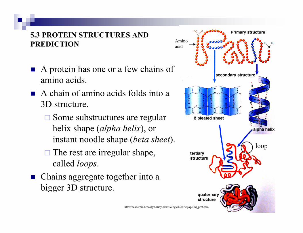
5.3 PROTEIN STRUCTURES AND PREDICTION Amino PREDICTION
A protein has one or a few chains of
acid
pamino acids.A chain of amino acids folds into a 3D t t3D structure.
Some substructures are regular helix shape (alpha helix), or e s ape (alpha helix), oinstant noodle shape (beta sheet).The rest are irregular shape,
ll d l
loop
called loops.Chains aggregate together into a bigger 3D structure.bigger 3D structure.
The prediction of protein secondary structure from its amino acid sequence can be considered as the problem of finding the correlation between the two objects. It can be studied in the framework of information theory.
The amino acid sequence can be regarded as an information source. The corresponding secondary structure can be considered as an information p g yreceiver. For an amino acid sequence of length N one can construct a secondary structure sequence of the same length written by three letters α, β, and c following the one-to-one correspondence between residue and secondary structure.
Let p (ai) be the probability of structure ai in the secondary structure sequence (ai = α, β, c) and let p (si) be the probability of amino acid si in h i (j 1 2 20) D fi l i f ithe protein (j = 1, 2, …, 20). Define average mutual information
∑∑∑ +−=−=i j
iiiiii
ii sapsapspapapYXHXHYXI )|(log)|())()(log)()|()();(
The maximum of H(X|Y) is H(X) which corresponds to no correlation between X and Y So the correlation between secondary structure (X) andbetween X and Y. So the correlation between secondary structure (X) and amino acid (Y) is defined by
),,,;,,(,)();(
1 YWCAscaXHYXIr ji L=== βα
where r1 takes values between 0 and 1:)(XH
INFORMATION THEORETIC APPROACHINFORMATION THEORETIC APPROACH
r1=0 means no correlation;r1=1 means the full determination of secondary structure by amino acid, this occurs in the case of p(ai|sj)=0 or 1 for all ai and sj.
The single peptide-structure correspondence can be easily extended to di-g p p p ypeptide (tri-peptide)-structure correspondence through residue numeration by shifting a window of width 2 (3). The above equations can be generalized in these cases. For the case of di-peptide-structure correspondence ai takes 9 confirmations, that is
αα, αβ, αc, βα, ββ, βc, cα, cβ.
sj takes 400 di-peptides in the above equations, that is,
AA AC WY YYAA, AC…., WY, YY.
INFORMATION THEORETIC APPROACHINFORMATION THEORETIC APPROACH
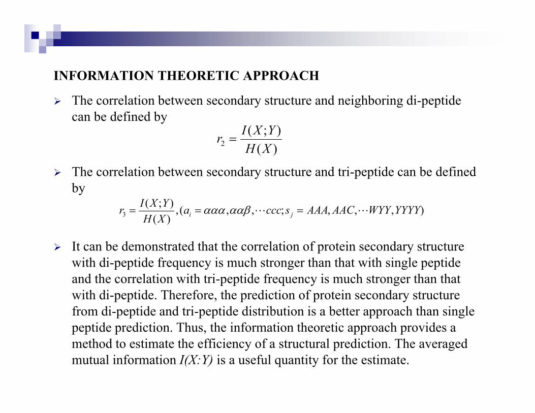
The correlation between secondary structure and neighboring di-peptide can be defined by
);( YXI
The correlation between secondary structure and tri-peptide can be defined
)();(
2 XHYXIr =
by ),,,;,,(,
)();(
3 YYYYWYYAACAAAscccaXHYXIr ji LL === ααβααα
It can be demonstrated that the correlation of protein secondary structure with di-peptide frequency is much stronger than that with single peptide and the correlation with tri-peptide frequency is much stronger than that p p q y gwith di-peptide. Therefore, the prediction of protein secondary structure from di-peptide and tri-peptide distribution is a better approach than single peptide prediction. Thus, the information theoretic approach provides a method to estimate the efficiency of a structural prediction. The averaged mutual information I(X:Y) is a useful quantity for the estimate.
TERTIARY STRUCTURE PREDICTION:POTENTIAL ENERGY SURFACE DEFINED BY FORCE FIELDSPOTENTIAL ENERGY SURFACE DEFINED BY FORCE FIELDS
Molecular Mechanics :
Consider a molecule with N atoms. The position of the i-th atom is denoted by the vector xi.
Describe the potential energy surface of a protein by molecular mechanics.
Molecular mechanics states that the potential energy of a protein can be approximated by the potential energy of the nuclei Therefore the energyapproximated by the potential energy of the nuclei. Therefore, the energy contribution of the electrons is neglected.
This approximation allows one to write the potential energy of a protein asThis approximation allows one to write the potential energy of a protein as a function of the nuclear coordinates.
TERTIARY STRUCTURE PREDICTION:POTENTIAL ENERGY SURFACE DEFINED BY FORCE FIELDSPOTENTIAL ENERGY SURFACE DEFINED BY FORCE FIELDS
Molecular Mechanics :A typical molecular modeling force field contains five types of potentials. These potentials correspond to deformation of
Covalent bond length Bond angles, Torsional motion associated with rotation about bonds, Electrostatic interactionElectrostatic interaction, van der Waals interaction.
The potential energy V=V(x) is a function of the atomic coordinate x of the molecule. The distance is measured in Ångstrom (Å), energy in kcal/mol,
d i t i it (D lt )
weakticelectrostatorsionanglelengh)(
and mass in atomic mass unit (Dalton).
TERTIARY STRUCTURE PREDICTION:POTENTIAL ENERGY SURFACE DEFINED BY FORCE FIELDSPOTENTIAL ENERGY SURFACE DEFINED BY FORCE FIELDS
Th b d l th t ti l i i bThe bond length potential is given by
∑ −=
b dji
ijlengh rrkV,
200 )(
Where rij=||xi-xj|| is the bond length, r0 is the reference bond length, and k0is a force constant. Reference bond lengths and force constants depend on
bonds
g pthe bond type. The bond potential corresponds to covalent bond deformation. The bond length deformations are sufficiently small at ordinary temperatures and in the absence of chemical reactions. The bond deformation energy between the i-th and j-th atom is given by a harmonic potential
2)( rrk 00 )( rrk ij −
TERTIARY STRUCTURE PREDICTION:POTENTIAL ENERGY SURFACE DEFINED BY FORCE FIELDSPOTENTIAL ENERGY SURFACE DEFINED BY FORCE FIELDS
The bond angle potential is given by
Wh θ i th f b d l d k i f t t R f
∑ −=
angle
angle kVθ
θθ 200 )(
Where θ0 is the reference bond angle and k0 is a force constant. Reference bond angle and force constant depend on the type of atom involved. The angle θ between the bonds p = xj-xi and r = xk - xj is given by
].,0[,||||||||
.)cos( πθθ ∈=rp
rp
The bond angle potential corresponds to angle deformation. Bond angle deformations are sufficiently small at ordinary temperatures and in the absence of chemical reactions.
TERTIARY STRUCTURE PREDICTION:POTENTIAL ENERGY SURFACE DEFINED BY FORCE FIELDSPOTENTIAL ENERGY SURFACE DEFINED BY FORCE FIELDS
The potentials for bond length and bond angle deformation are considered as the hard degrees of freedom in a molecular system in the sense thatas the hard degrees of freedom in a molecular system in the sense that considerable energy is necessary to cause significant deformation from their reference values. The most variation in structure and relative energy comes from the remaining potential energy terms.comes from the remaining potential energy terms.
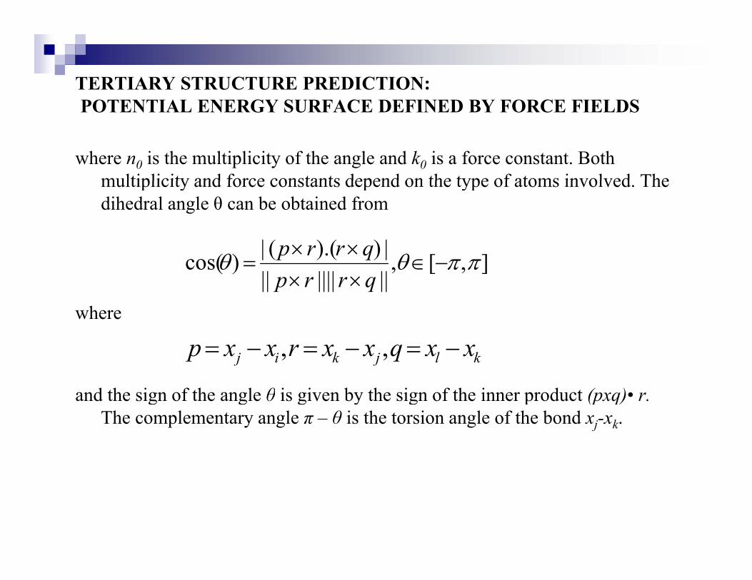
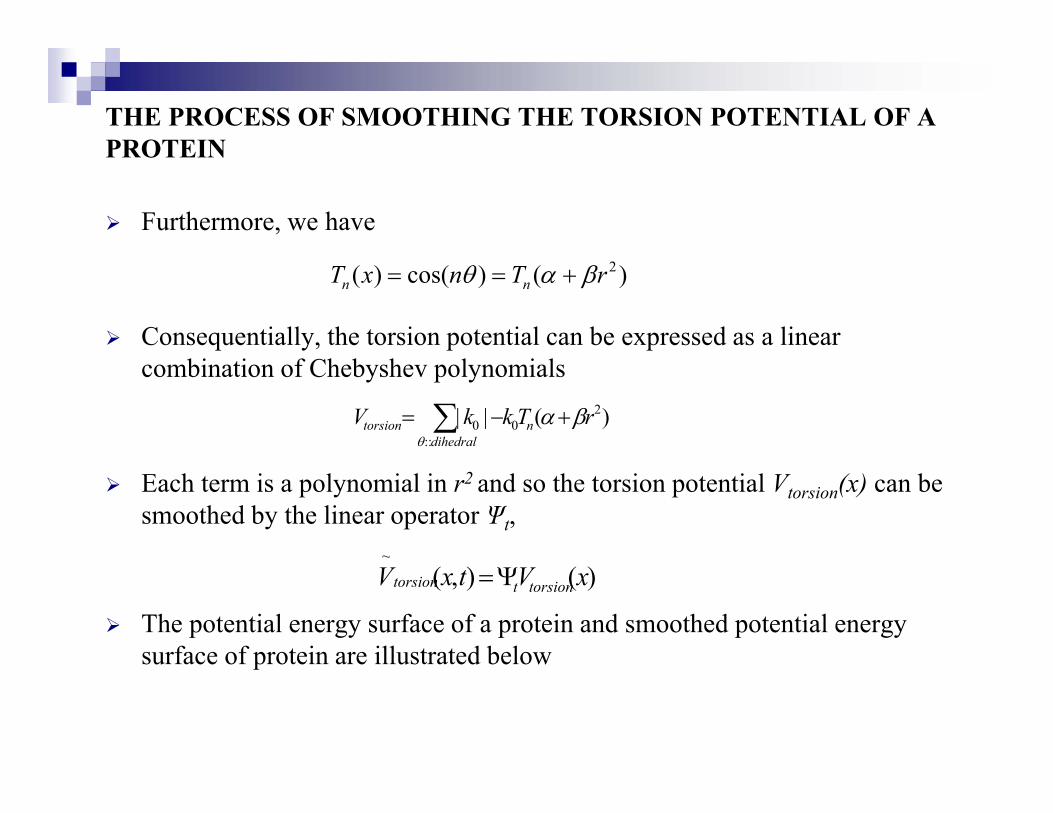
The torsion potential corresponds to the barriers of bond rotation which involves the dihedral angles of the rotatable bonds. The barriers of torsion can be expressed as a series of cosine functions. The mathematical expression for the torsion potential is given by
∑ 2
where n0 is the multiplicity of the angle and k0 is a force constant Both
∑ −=dihedral
torsion nkkV::
2000 )cos(||
θ
θ
where n0 is the multiplicity of the angle and k0 is a force constant. Both multiplicity and force constants depend on the type of atoms involved. The dihedral angle θ can be obtained from
TERTIARY STRUCTURE PREDICTION:POTENTIAL ENERGY SURFACE DEFINED BY FORCE FIELDSPOTENTIAL ENERGY SURFACE DEFINED BY FORCE FIELDS
where n0 is the multiplicity of the angle and k0 is a force constant. Both multiplicity and force constants depend on the type of atoms involved Themultiplicity and force constants depend on the type of atoms involved. The dihedral angle θ can be obtained from
|)).((| ×× qrrp
where
],[,|||||||||)).((|)cos( ππθθ −∈
××××
=qrrpqrrp
and the sign of the angle θ is given by the sign of the inner product (pxq)• r.
kljkij xxqxxrxxp −=−=−= ,,
and the sign of the angle θ is given by the sign of the inner product (pxq) r.The complementary angle π – θ is the torsion angle of the bond xj-xk.
TERTIARY STRUCTURE PREDICTION:POTENTIAL ENERGY SURFACE DEFINED BY FORCE FIELDSPOTENTIAL ENERGY SURFACE DEFINED BY FORCE FIELDS
The electrostatic potential corresponds to the nonbounded interaction between the charged atoms in a molecule The interaction is attractive whenbetween the charged atoms in a molecule. The interaction is attractive when the charges have opposite sign and repulsive when the charges have the same sign. The electrostatic potential of a molecule is given by
∑<
=
atomsji ij
jiticelectrosta r
qqV
04πδ
where qi is the point charge of the i-th atom and δ0 is the dielectric constant of vacuum, and rij is the distance between i-th and j-th atoms.
TERTIARY STRUCTURE PREDICTION:POTENTIAL ENERGY SURFACE DEFINED BY FORCE FIELDSPOTENTIAL ENERGY SURFACE DEFINED BY FORCE FIELDS
The van der Waals potential corresponds to the interaction between nonbounded atoms in a molecule This interaction comes from attractivenonbounded atoms in a molecule. This interaction comes from attractive and repulsive forces. The van der Waals potential is given by
∑⎥⎥⎦
⎤
⎢⎢⎣
⎡⎟⎟⎠
⎞⎜⎜⎝
⎛−⎟
⎟⎠
⎞⎜⎜⎝
⎛= ijji
weak rB
rA
V 612
Where Aij and Bij are given by< ⎥⎦⎢⎣
⎟⎠
⎜⎝
⎟⎠
⎜⎝atoms
ji ijij rr
6)(1jiijij RRBA += )(
2 jiijij
jji
ji
eij NNi
em
Bαα
ααπδ +
=h1
41
23
0
where e is the electron charge, ħ is the reduced Planck constant, me is the electron mass, αi is the polarizability of the ith atom, Ni is the effective number of outer shell electrons in the ith atom. Ri is the van der Waalsnumber of outer shell electrons in the ith atom. Ri is the van der Waals radius of the i-th atom.
CONFORMATIONAL SEARCH METHODS
The objective of conformational search is to find all preferred conformations of a moleculeconformations of a molecule.
The conformational search of the global minimum energy surface of a protein from the amino acid sequence is one of the challenging problems in p q g g pbioinformatics.
In recent years, several optimization approaches to solve this problem have appeared in the literature. The most common approach is to model the protein surface by using a force field.
Th l h i t d fi th t th t i li d hThe general scheme is to define a smooth operator that is linear and each term of the potentials can be separately smoothed.
THE PROCESS OF SMOOTHING THE TORSION POTENTIAL OF A PROTEINPROTEIN
Express the dihedral angles by distances. We assume that bond lengths and bond angles are fixed to their reference values Then the cosine of abond angles are fixed to their reference values. Then the cosine of a dihedral angle θ can be expressed by the distance r = ||xl-xi|| of the first and last of the involved atoms:
where α and β are constants depending on the reference bond lengths and f b d l I l ( θ) f lti l dih d l l
2)cos( rβαθ +=
reference bond angles. In general cos (nθ) of a multiple dihedral angle can be represented as a Chebyshev polynomial in cos (θ), which is a polynomial in r2.
Let x = cos (θ), then the Chebyshev polynomials can be written as
)arccos(cos()cos()( xnnxTn == θ )(()()(n
THE PROCESS OF SMOOTHING THE TORSION POTENTIAL OF A PROTEINPROTEIN
Furthermore, we have
Consequentially, the torsion potential can be expressed as a linear
)()cos()( 2rTnxT nn βαθ +==
combination of Chebyshev polynomials
)(||::
200∑ +−=
dihedralntorsion rTkkV
θ
βα
Each term is a polynomial in r2 and so the torsion potential Vtorsion(x) can be smoothed by the linear operator Ψt,
~
The potential energy surface of a protein and smoothed potential energy surface of protein are illustrated below
)(),( xVtxV torsionttorsion Ψ=
surface of protein are illustrated below
Potential energy surface of protein
The process of smoothing the torsion potential of a protein
Smoothed potential energy surface of protein
The process of smoothing the torsion potential of a protein
5.4 STATISTICAL APPROACH AND DISCUSSIONS
Fold Recognition
Proteins may have similar tertiary structures even if their primary structures are not sufficiently similar or different.
This observation has led to the hypothesis that there are only a limited number of significantly distinct tertiary structures.
The main goal of fold recognition is to predict the tertiary structure of a protein from its amino acid sequence by finding the best match between the amino acid sequence and some tertiary structure in a protein database. q y p
A basic approach to fold recognition is comparative modeling.
5.4 STATISTICAL APPROACH AND DISCUSSIONS
Fold Recognition
Let A be the amino acid sequence of a protein with unknown tertiary structure, align the sequence A to the primary structures of all proteins in th d t b f t ti t i t t S th A b tthe database of tertiary protein structures. Suppose the sequence A best aligns to the primary structure of B. This sequence alignment can be used to infer the structural alignment. For example, if the residue ai of A aligns with the residue b of B then the position of the residue a in the unknownwith the residue bj of B, then the position of the residue ai in the unknown tertiary structure is defined as the position of the residue bj in the tertiary structure in the database. Subsequences of the sequence of A aligned with a series of blanks of the sequence of B are modeled as coil region.series of blanks of the sequence of B are modeled as coil region.
Fold Recognition
Threading predicted 1D structure profiles into known 3D structures: (1) Input sequence; (2) Generate sequence alignment; ( ) p q ; ( ) q g ;(3) Predict 1D structure; (4) Align predicted and known structure(s)
3D PROFILE-SEQUENCE ALIGNMENT
A more sophisticated approach to fold recognition makes use of the method of 3D profile sequence alignment For this we make use of both sequenceof 3D profile-sequence alignment. For this, we make use of both sequence database and protein database.
Let A be a sequence of amino acid and P be the 3D profile of a protein. q p pWe align A to P. Let σ (P, A) be the corresponding alignment score. To estimate the significance of these alignment scores, we align the protein with 3D g g , g pprofile P against all amino acid sequences of a sequence database. The Z score for aligning the amino acid sequence A to the protein with 3D profile P is given byp g y
)()(),(),(
PPAPAPZ
σμσ −
=)(
3D PROFILE-SEQUENCE ALIGNMENT
where µ(P) is the mean score of alignment scores given by
with M as the number of sequences in the sequence database, and σ (P) is the
∑=A
APM
P ),(1)( σμ
standard deviation of the scores given by
2))()((1)( ∑ −= PaPP μσσ
A high Z score Z(P, Z) may indicate that amino acid sequence A has similar tertiary structure as the protein with the 3D profile P.
))(),(()( ∑=A
PaPM
P μσσ
tertiary structure as the protein with the 3D profile P.
5.5. CHALLENGES AND PERSPECTIVES
The sequences of similar structures in PDB, how to identify the correct templates and how to refine the template structure closer to the native.
The sequences without appropriate templates, how to build models of correct topology from scratch.
Protein function is closely related to its 3D structure and applications.
d di i d
calcium
E.g., mad-cow disease is due to PrP misfolding.E.g., calcium atoms bind to good-shape-loopsshape-loops.