1

Mathematics Review

Applied Computational Fluid Dynamics

Instructor: André Bakker

http://www.bakker.org© André Bakker (2002-2006)

2

Vector Notation - 1

=

=.

=x

=

ii yxYXproduct:("inner")Scalar =⋅rr

ZYXproduct:("outer")Vectorrrr

=×

jiij yxaAYXproducttensorDyadic ==rrrr

:)"("

ii fxyYfXtion:Multiplica ==rv

jiij baBAproduct:("inner")dotDouble =rrrr

: =:

3

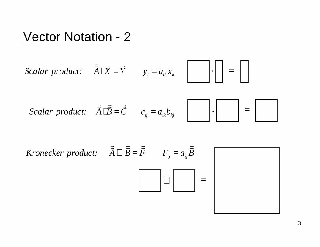
Vector Notation - 2

=.

=.

kiki xayYXAproduct:Scalar ==⋅rrrr

kjikij bacCBAproduct:Scalar ==⋅rrrrrr

=⊗

BaFFBAproduct:kerKronec ijij

rrrrrrrr==⊗

4

• The gradient of a scalar f is a vector:

Similarly, the gradient of a vector is a second order tensor, and the gradient of a second order tensor is a third order tensor.

• The divergence of a vector is a scalar:

Gradients and divergence

kjiz

f

y

f

x

fffgrad

∂∂+

∂∂+

∂∂=∇=

z

A

y

A

x

Adiv zyx

∂∂+

∂∂

+∂∂=∇= .AA

=

=.

5

• The curl (“rotation”) of a vector v(u,v,w) is another vector:

Curl

∂∂−

∂∂

∂∂−

∂∂

∂∂−

∂∂=×∇==

y

u

x

v

x

w

z

u

z

v

y

wrotcurl ,,vvv

=x

6

Definitions - rectangular coordinates

kjiA

∂∂−

∂∂

+

∂∂−

∂∂+

∂∂

−∂∂=×∇

y

A

x

A

x

A

z

A

z

A

y

A xyzxyz

2

2

2

2

2

22

z

f

y

f

x

ff

∂∂+

∂∂+

∂∂=∇

kjiA zyx AAA 2222 ∇+∇+∇=∇

kjiz

f

y

f

x

ff

∂∂+

∂∂+

∂∂=∇

z

A

y

A

x

A zyx

∂∂+

∂∂

+∂∂=∇.A

7

Identities

fggfgf ∇+∇=∇ )(

B)(AA)(B)B(A)A(BB)(A ×∇×+×∇×+∇⋅+∇⋅=⋅∇

)()()( AAA ⋅∇+⋅∇=⋅∇ fff

B)(AABBA ×∇⋅−×∇⋅=×⋅∇ )()(

)()()( AAA ×∇+×∇=×∇ fff

A)B(B)A()B(A)A(BB)(A ⋅∇−⋅∇+∇⋅−∇⋅=××∇

8

Identities

AA)(A 2∇−⋅∇∇=×∇×∇

k

j

i)B(A

∂∂+

∂∂+

∂∂+

∂∂

+∂

∂+

∂∂

+

∂∂+

∂∂+

∂∂=∇⋅

z

BA

y

BA

x

BA

z

BA

y

BA

x

BA

z

BA

y

BA

x

BA

zz

zy

zx

yz

yy

yx

xz

xy

xx

τvolumeboundswhichsurfacetheisSwhere

d

fdf

S

S

∫∫

∫ ∫

×−=×∇

=∇

daAA

da

τ

τ

τ

τ

)(

9

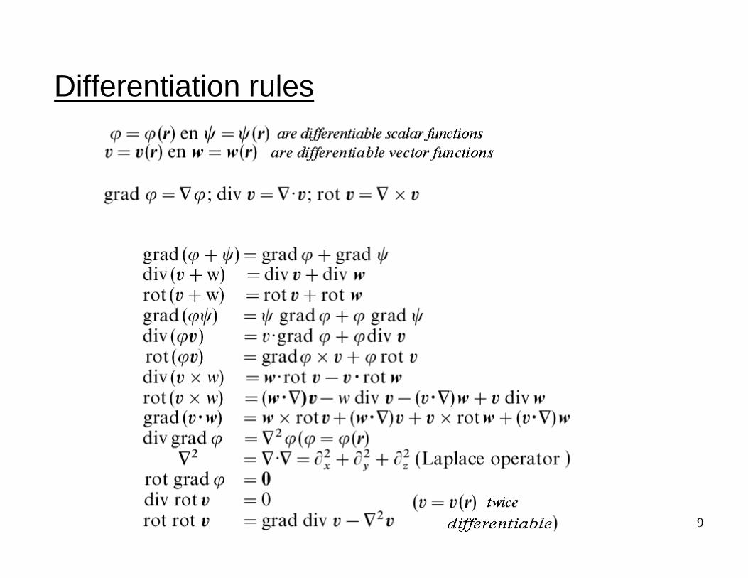
Differentiation rules

10

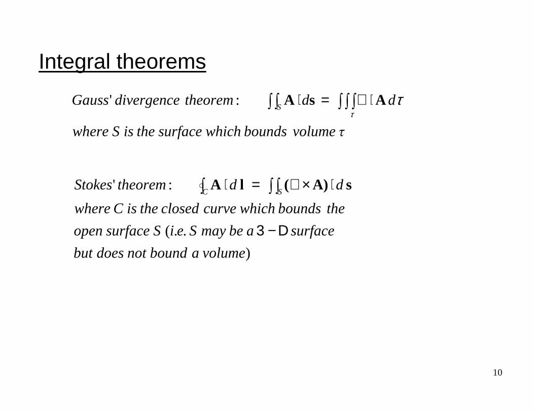
Integral theorems

τvolumeboundswhichsurfacetheisSwhere

ddtheoremdivergenceGaussS ∫ ∫ ∫∫ ∫ ⋅∇=⋅

ττAsA:'

)

..(

:'

volumeaboundnotdoesbut

surfaceabemaySeiSsurfaceopen

theboundswhichcurveclosedtheisCwhere

ddtheoremStokesSC

D3 −

⋅×∇=⋅ ∫ ∫∫ sA)(lA

11

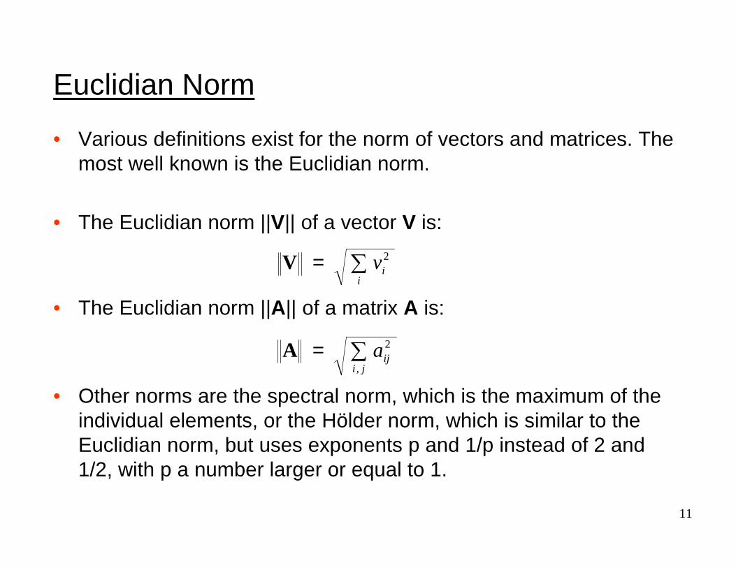
Euclidian Norm

• Various definitions exist for the norm of vectors and matrices. The most well known is the Euclidian norm.

• The Euclidian norm ||V|| of a vector V is:

• The Euclidian norm ||A|| of a matrix A is:

• Other norms are the spectral norm, which is the maximum of the individual elements, or the Hölder norm, which is similar to the Euclidian norm, but uses exponents p and 1/p instead of 2 and 1/2, with p a number larger or equal to 1.

∑=ji

ija,

2A

∑=i

iv2V

12

Matrices - Miscellaneous

• The determinant of a matrix A with elements aij and i=3 rows and j=3 columns:

• A diagonal matrix is a matrix where all elements are zero except a11, a22, and a23. For a tri-diagonal matrix also the diagonals above and below the main diagonal are non-zero, while all other elements are zero.

• Triangular decomposition is expressing A as the product LU with L a lower-triangular matrix (elements above diagonal are 0) and U an upper triangular matrix.

• The transpose AT has elements a’ij=aji. A matrix is symmetric if AT =A.• A sparse matrix is a matrix where the vast majority of elements is zero

and only few elements are non-zero.

322311332112312213322113312312332211

333231

232221

131211

det aaaaaaaaaaaaaaaaaa

aaa

aaa

aaa

−−−++=

=

A

A

13

Matrix invariants - 1• An invariant is a scalar property of a matrix that is independent of the coordinate

system in which the matrix is written.• The first invariant I1 of a matrix A is the trace tr A. This is simply the sum of the

diagonal components: I1 = tr A = a11 + a22 + a33

• The second invariant is:

• The third invariant is the determinant of the matrix: I3 = det A.

• The three invariants are the simplest possible linear, quadratic, and cubic combinations of the eigenvalues that do not depend on their ordering.

3313

3111

2212

2111

3323

32222 aa

aa

aa

aa

aa

aaI ++=

14

Matrix invariants - 2• Using the previous definitions we can form infinitely many other variants, e.g:

• In CFD literature, one will sometimes encounter the following alternative definitions of the second invariant (which are derived from the previous definitions):

– For symmetric matrices:

I2 = (1/2)*[(tr A)2 - tr A2] = a11a22 + a22a33 + a33a11

or

I2 = (1/6) * [ (a11-a22)2 + (a22-a33)2 + (a33-a11)2 ] + a122 + a23

2+ a312

– The Euclidian norm: ∑==ji

ijaI,

22 A

( )ikik

ii

aaII

aI

=−=

221

221

2

15

Gauss-Seidel method

• The Gauss-Seidel method is a numerical method to solve the following set of linear equations:

• We first make an initial guess for x1:

• The superscript 1 denotes the 1st iteration. • Next, using x1

1:

NNNNNNN

NN

Cxaxaxaxa

Cxaxaxaxa

=++++

=++++

.....

.....

332211

11313212111

MMM

11

111 a

Cx =

)(1 1

121

2222

212 xa

aa

Cx −=

16

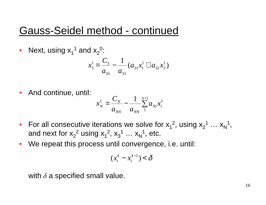
Gauss-Seidel method - continued

• Next, using x11 and x2

0:

• And continue, until:

• For all consecutive iterations we solve for x12, using x2

1 … xN1,

and next for x22 using x1

2, x31 … xN

1, etc.• We repeat this process until convergence, i.e. until:

with δ a specified small value.

)(1 1

2321131

3333

313 xaxa

aa

Cx +−=

∑−

−=1

1

11 1 n

iNi

NNNN

NN xa

aa

Cx

δ<− − )( 1ki

ki xx

17

Gauss-Seidel method - continued

• It is possible to improve the speed at which this system of equations is solved by applying overrelaxation, or improve the stability if the system does not converge by applying underrelaxation.

• Say at iteration k the value of xi equals xik. If applying the Gauss-

Seidel method, the value for iteration k+1 would be xik+1, then,

instead of using xik+1, we consider this to be a predictor.

• We then calculate a corrector as follows:

• Here R is the relaxation factor (R>0). If R<1 we use underrelaxation and if R>1 we use overrelaxation.

• Next we recalculate xik+1as follows:

)( 1 ki

ki xxRcorrector −= +

correctorxx ki

ki +=+1

18

Gauss elimination

• Consider the same set of algebraic equations shown in the Gauss-Seidel discussion. Consider the matrix A:

• The heart of the algorithm is the technique for eliminating all the elements below the diagonal, i.e. to replace them with zeros, tocreate an upper triangular matrix:

=

nnnn

n

n

aaa

aaa

aaa

L

MOMM

L

L

21

22221

11211

A

=

nn

n

n

a

aa

aaa

L

MOMM

L

L

00

0 222

11211

U

19

Gauss elimination - continued

• This is done by multiplying the first row by a21/a11 and subtracting it from the second row. Note that C2 then becomes C2-C1a21/a11.

• The other elements a31 through an1 are treated similarly. Now all elements in the first column below a11 are 0.

• This process is then repeated for all columns.• This process is called forward elimination.• Once the upper diagonal matrix has been created, the last

equation only contains one variable xn, which is readily calculated as xn=Cn/ann.

• This value can then be substituted in equation n-1 to calculate xn-1and this process can be repeated to calculate all variables xi. This is called backsubstitution.

• The number of operations required for this method increases proportional to n3. For large matrices this can be a computationally expensive method.

20

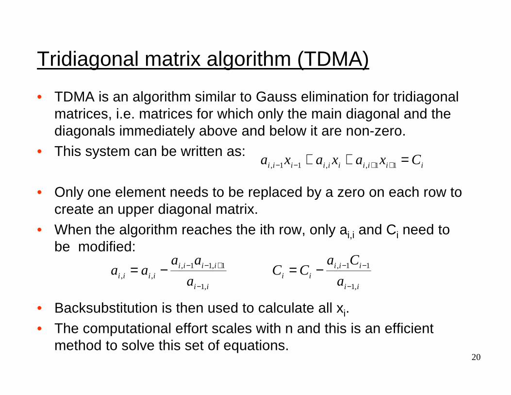
Tridiagonal matrix algorithm (TDMA)

• TDMA is an algorithm similar to Gauss elimination for tridiagonal matrices, i.e. matrices for which only the main diagonal and thediagonals immediately above and below it are non-zero.

• This system can be written as:

• Only one element needs to be replaced by a zero on each row to create an upper diagonal matrix.

• When the algorithm reaches the ith row, only ai,i and Ci need to be modified:

• Backsubstitution is then used to calculate all xi.• The computational effort scales with n and this is an efficient

method to solve this set of equations.

iiiiiiiiii Cxaxaxa =++ ++−− 11,,11,

ii

iiiii

ii

iiiiiiii a

CaCC

a

aaaa

,1

11,

,1

1,11,,,

−

−−

−

+−− −=−=

21

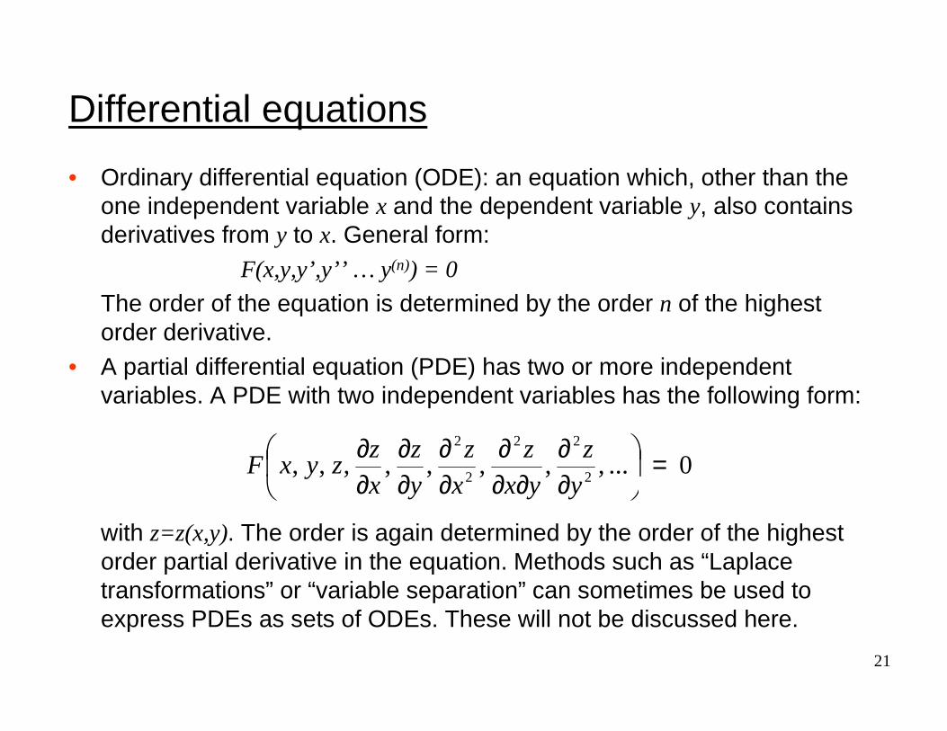
Differential equations

• Ordinary differential equation (ODE): an equation which, other than the one independent variable x and the dependent variable y, also contains derivatives from y to x. General form:

F(x,y,y’,y’’ … y(n)) = 0

The order of the equation is determined by the order n of the highest order derivative.

• A partial differential equation (PDE) has two or more independent variables. A PDE with two independent variables has the following form:

with z=z(x,y). The order is again determined by the order of the highest order partial derivative in the equation. Methods such as “Laplace transformations” or “variable separation” can sometimes be used to express PDEs as sets of ODEs. These will not be discussed here.

0...,,,,,,,,2

22

2

2

=

∂∂

∂∂∂

∂∂

∂∂

∂∂

y

z

yx

z

x

z

y

z

x

zzyxF

22

Classification of partial differential equations

• A general partial differential equation in coordinates x and y:

• Characterization depends on the roots of the higher order (here second order) terms:– (b2-4ac) > 0 then the equation is called hyperbolic.– (b2-4ac) = 0 then the equation is called parabolic.– (b2-4ac) < 0 then the equation is called elliptic.

• Note: if a, b, and c themselves depend on x and y, the equationsmay be of different type, depending on the location in x-y space. In that case the equations are of mixed type.

02

22

2

2

=++∂∂+

∂∂+

∂∂+

∂∂∂+

∂∂

gfy

ex

dy

cyx

bx

a φφφφφφ

23

Origin of the terms

• The origin of the terms “elliptic,” “parabolic,” or “hyperbolic used to label these equations is simply a direct analogy with the case for conic sections.

• The general equation for a conic section from analytic geometry is:

where if– (b2-4ac) > 0 the conic is a hyperbola.– (b2-4ac) = 0 the conic is a parabola. – (b2-4ac) < 0 the conic is an ellipse.

022 =+++++ feydxcybxyax

24

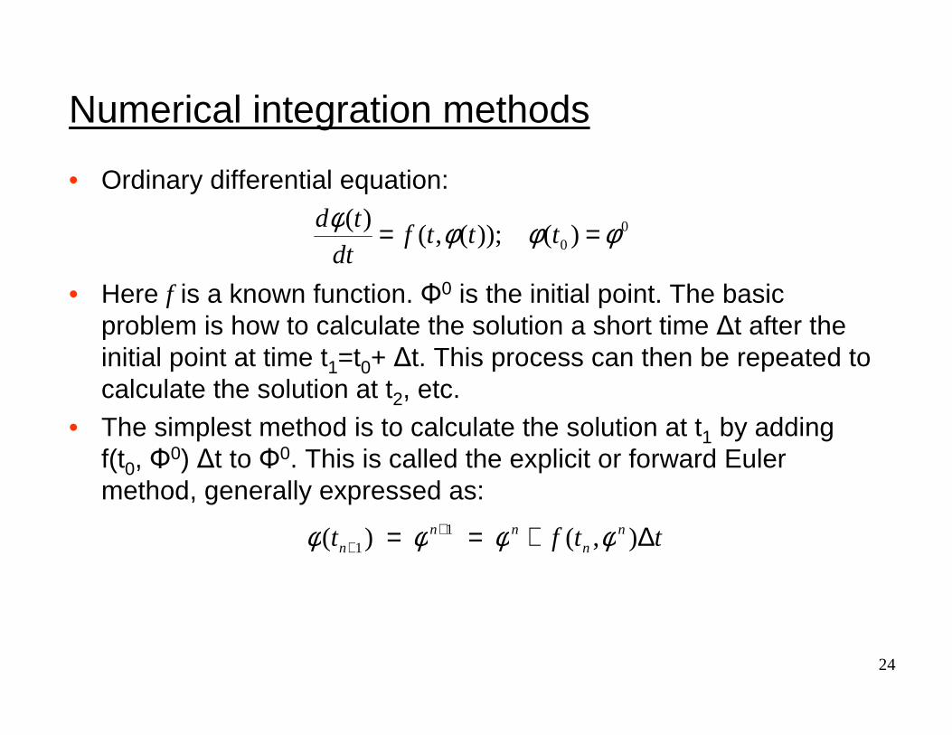
Numerical integration methods

• Ordinary differential equation:

• Here f is a known function. Φ0 is the initial point. The basic problem is how to calculate the solution a short time ∆t after the initial point at time t1=t0+ ∆t. This process can then be repeated to calculate the solution at t2, etc.

• The simplest method is to calculate the solution at t1 by adding f(t0, Φ

0) ∆t to Φ0. This is called the explicit or forward Euler method, generally expressed as:

00)());(,(

)( φφφφ == tttfdt

td

ttft nn

nnn ∆+== +

+ ),()( 11 φφφφ

25

Numerical integration methods

• Another method is the trapezoid rule which forms the basis of a popular method to solve differential equations called the Crank-Nicolson method:

• Methods using points between tn and tn+1 are called Runge-Kutta methods, which come in various forms. The simplest one is second-order Runge-Kutta:

tnn

tfnn

tfnn ∆++++=

+ )1,1

(),(2

11 φφφφ

),(

),(2

*2/12/1

1

*2/1

+++

+

∆+=

∆+=

nnnn

nn

nn

tft

tft

φφφ

φφφ

26

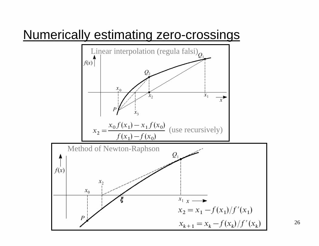
Numerically estimating zero-crossings

(use recursively)

Linear interpolation (regula falsi)

Method of Newton-Raphson

27

Jacobian

• The general definition of the Jacobian for n functions of nvariables is the following set of partial derivatives:

• In CFD, the shear stress tensor Sij = ∂Ui/ ∂xj is also called “the Jacobian.”

n

nnn

n

n

n

n

x

f

x

f

x

f

x

f

x

f

x

fx

f

x

f

x

f

xxx

fff

∂∂

∂∂

∂∂

∂∂

∂∂

∂∂

∂∂

∂∂

∂∂

=∂∂

...

............

...

...

),...,,(),...,,(

21

2

2

2

1

2

1

2

1

1

1

21

21

28

Jacobian - continued

• The Jacobian can be used to calculate derivatives from a function in one coordinate sytem from the derivatives of that same function in another coordinate system.

• Equations u=f(x,y), v=g(x,y), then x and y can be determined as functions of u and v (possessing first partial derivatives) as follows:

• With similar functions for xv and yv.• The determinants in the denominators are examples of the use of

Jacobians.

yx

yx

x

yx

yx

y

yx

yx

gg

ffg

u

y

gg

ff

g

u

x

yggxggyxgv

xffyffyxfu

−=∂∂=

∂∂

∂∂=∂∂==

∂∂=∂∂==

/;/);,(

/;/);,(

29

Eigenvalues• If an equation with an adjustable parameter has non-trivial

solutions only for specific values of that parameter, those values are called the eigenvalues and the corresponding function the eigenfunction.

• If a differential equation with an adjustable parameter only has a solution for certain values of that parameter, those values are called the eigenvalues of the differential equation.

• For an nxn matrix A, for the equation Az = λz, then z is an eigenvector and λ is an eigenvalue.

• The eigenvalues are the n roots of the characteristic equation

det(λI-A) = λn+p1λn-1+…+pn = 0

• (λI-A) is the characteristic matrix of A.• The polynomial is called the characteristic polynomial of A.

• The product of all the eigenvalues of A is equal to det A.

• The sum of all the eigenvalues is equal to tr A.• The matrix is singular if at least one eigenvalue is zero.

30

Taylor series

• Let f(x) have continuous derivatives up to the (n+1)st order in some interval containing the point a. Then:

...)(!

)(....)(

!2)(''

)(!1

)(')()( 2 +−++−+−+= n

n

axn

afax

afax

afafxf

31

Error function

• The error function is defined as:

• It is the integral of the Gaussian (“normal”) distribution. It is usually calculated from series expansions.

• Properties are:

)(1)(

2)(

0

2

zerfzerfcfunction:erroraryComplement

dtezerffunction:Errorz t

−=

= ∫−

π

( )2exp2)(

)()(

1)(

0)0(

zdz

zerfd

zerfzerf

erf

erf

−=

−−==∞=

π

32

Permutation symbol

• The permutation symbol ekmn resembles a third-order tensor.

• If the number of transpositions required to bring k, m, and n in the form 1, 2, 3 is even then ekmn=1.

• If the number of transpositions required to bring k, m, and n in the form 1, 2, 3 is odd then ekmn=-1.

• Otherwise ekmn=0.

• Thus:

• Instead of ekmn the permutation symbol is also often written as εkmn

zeroareelementsotherall

eee

eee

1

1

213321132

312231123

−======

33

Correlation functions

• Continuous signals.• Let x(t) and y(t) be two signals. Then the correlation function Φxy(t) is

defined as:

• The function Φxx(t) is usually referred to as the autocorrelation function of the signal, while the function Φxy(t) is usually called the cross-correlation function.

• Discrete time series.• Let x[n] and y[n] be two real-valued discrete-time signals. The

autocorrelation function Φxx[n] of x[n] is defined as:

• The cross-correlation function is defined as:

∫∞

∞−+= τττφ dytxtxy )()()(

∑∞+

−∞=+=

mxx mxnmxn ][][][φ

∑∞+

−∞=+=

mxy mynmxn ][][][φ

34

• Fourier transforms are used to decompose a signal into a sum of complex exponentials (i.e. sinusoidal signals) at different frequencies.

• The general form is:

• X(ω) is the Fourier transform of x(t). It is also called the spectrum because it shows the amplitude (“energy”) associated with each frequency ω present in the signal. X(ω) is a complex function with real and imaginary parts. The magnitude |X(ω)| is also called the power spectrum.

• Slightly different forms exist for continuous, discrete, periodic, and aperiodic signals.

ωω

ωωπ

ω

ω

detxX

deXtx

ti

ti

−∞

∞−

∞

∞−

∫

∫

=

=

)()(

)(21

)(

Fourier transforms