THE SOLUTION OF A VARIABLE BOUNDARY PROBLEM

Co. H. Tran - Phong .T. Ngo

Faculty of Mathematics, University of Natural Sciences - VNU-HCM coth123@math.com & cohtran@math.com

Copyright 2007August 16 2007

NOTE: This worksheet demonstrates Maple's capabilities in researching the numerical and graphical solution of the variable boundary problem of a thick-walled cylinder of material enclosed in a thin metallic shell . All rights reserved. Copying or transmitting of this material without the permission of the authors is not allowed . Abstract : The relations between stress and strain in linear viscoelastic theory are discussed from the viewpoint of application to problems of stress analysis. This consideration includes some important differences from the estimation of linear viscoelastic laws for the representation of material properties , and the integral operators expressing the creep function or relaxation function can be applied . By using of the differential operator for the relation between stress and strain it is usually most convenient to solve some problems which have the variable boundary .

Problem Definition

We consider a thick-walled cylinder of material enclosed in a thin metallic shell . ( Fig. 1)

( Fig 1 ) . The outer radius of cylinder : b ; the thickness of the metallic shell : h .

The inner radius a is assumed by : a(t) , satisfied the condition . The varying pressure influences upon the inner surface is a given function q(t) . Notice that the tube and shell are under the plain strain conditions and the material is incompressible.

By setting : the radical stress , : the circular stress ,

: the radical displacement ,

are the deformation respectively .

The diferential equation of equilibrium: Bywhat we introduce in (I) it follows that the diferential equation of equilibrium can be written consequently :

(1) In this case we have the law of viscoelasticity relation :

(2)

At the inner boundary : r = a , = -q(t) The circular deformation of the cylinder of material obtained by integrating :

(3) Here E and are the elastic constants of the shell material .

The second boundary condition : e = (b) Because of incompressibility of material and zero axial strain :

it follows that : , , (4.29)

From (2) we obtain : (4)

By substituting (4) to (1) , the deduction can be rewritten : (5)

Integrating (5) gives : (6)

By using the condition : r = a , = - q (t)

then and (7) The relation (6) becomes :

(8)

Consider the second boundary condition : , then we arrive at the integral equation for k(t) :

(9) inwhich we set up :

(10) . The equation (9) can be considered as especial case of the general formation :

(11) The authors of [2] have considered the simplest case of a viscoelastic body expressed by formular :

(12)

Here are the given constants defined by experiments on material . The equation (9) now becomes differential for k(t) .

(13) From (13) , we find out the solution k(t) correspondently with choosing the functions a(t) and q(t) .For examples , some authors have taken :

(14) Here q = const . [ = E in case of elasticity , = 3 in case of Newton's fluid ] . By integrating (13) we obtain the solution of the viscoelasticity problem . In generally the differential equation for k(t) would be established in symbolic form by using the operator :

(15)

Numerical and graphical solution:

Here we have used the parameters :

(13) canbe rewitten as the following :

The analytic solution :

> restart; with(DEtools): a(t)=a[0]/sqrt(1-delta*t); eq:=alpha*(1/a(t)^2-1/b^2)*diff(k(t),t)+(beta*(1/a(t)^2-1/b^2)-1/(b^2*c))*k(t)=q(t); eq:=subs(a(t)=a[0]/sqrt(1-delta*t),eq); eq:=subs(q(t)=q[0],eq); nok:=dsolve(eq,k(t));

a ( t ) =a0

1K d t

eq :=a ⎛⎝1

a ( t )2 K1b2⎞⎠ 0 d

dt k ( t )1

C ⎛⎝b ⎛⎝

1a ( t )2 K

1b2⎞⎠ K

1b2 c

⎞⎠ k ( t ) = q ( t )

eq :=a ⎛⎜⎝1 K d t

a02 K

1b2⎞⎟⎠

0 ddt

k ( t )1C

⎛⎜⎝b ⎛⎜⎝

1 K d ta0

2 K1b2⎞⎟⎠K

1b2 c

⎞⎟⎠

k ( t ) = q ( t )

eq :=a ⎛⎜⎝1 K d t

a02 K

1b2⎞⎟⎠

0 ddt

k ( t )1C

⎛⎜⎝b ⎛⎜⎝

1 K d ta0

2 K1b2⎞⎟⎠K

1b2 c

⎞⎟⎠

k ( t ) = q0

nok := k ( t ) =

⎛⎜⎜⎜⎜⎜⎜⎝

⌠⎮⎮⎮⎮⎮⎮⌡

Kq0 a0

2 b2 0Kb2 C b2 d t C a021

⎛⎜⎝K

c a b2 dK a02

c a b2 d

⎞⎟⎠

e0 b t

a1

adt

C _C1

⎞⎟⎟⎟⎟⎟⎟⎠

e0Kb t

a1

0Kb2 C b2 d t C a021

⎛⎜⎝K

a02

c a b2 d

⎞⎟⎠

> restart; with(DEtools): cof := 1000: eq := alpha*(1/a(t)^2-1/b^2)*(diff(k(t), t))+(beta*(1/a(t)^2-1/b^2)-1/(b^2*c))*k(t) = q(t);eq := subs(a(t) = a[0]/sqrt(1-delta*t), eq); eq := subs(q(t) = q[0], eq); nok := dsolve(eq, k(t)); nok := evalf(subs(c = 1.2, delta = 0.5e-2, alpha = .5, b = 1.5, a[0] = 1, beta = 2, q[0] = 1, nok), 3); u := k(t)/(r*cof);

cof := 1000

eq :=a ⎛⎝1

a ( t )2 K1b2⎞⎠ 0 d

dt k ( t )1

C ⎛⎝b ⎛⎝

1a ( t )2 K

1b2⎞⎠ K

1b2 c

⎞⎠ k ( t ) = q ( t )

eq :=a ⎛⎜⎝1 K d t

a02 K

1b2⎞⎟⎠

0 ddt

k ( t )1C

⎛⎜⎝b ⎛⎜⎝

1 K d ta0

2 K1b2⎞⎟⎠K

1b2 c

⎞⎟⎠

k ( t ) = q ( t )

eq :=a ⎛⎜⎝1 K d t

a02 K

1b2⎞⎟⎠

0 ddt

k ( t )1C

⎛⎜⎝b ⎛⎜⎝

1 K d ta0

2 K1b2⎞⎟⎠K

1b2 c

⎞⎟⎠

k ( t ) = q0

nok := k ( t ) =

⎛⎜⎜⎜⎜⎜⎜⎝

⌠⎮⎮⎮⎮⎮⎮⌡

Kb2 0Kb2 C b2 d t C a0

21

⎛⎜⎝

Kc a b2 dC a02

c a b2 d

⎞⎟⎠

a02 q0 e

0 b ta1

adt

C _C1

⎞⎟⎟⎟⎟⎟⎟⎠

e0Kb t

a1

0Kb2 C b2 d t C a021

⎛⎜⎝K

a02

c a b2 d

⎞⎟⎠

nok := k ( t ) = 1(K1.25C 0.0112 t )148.

⎛⎜⎝⎛⎜⎝⌠⎮⌡K

4.50 (K1.25C 0.0112 t )147. e ( 4.00 t ) dt C _C1⎞⎟⎠

e (K4.00 t ) ⎞⎟⎠

u := 11000

k ( t )r

> k(t):=(int(-4.50*(-1.25+.112e-1*s)^147.*exp(4.00*s),s=0..t)+.22013e14)*exp(-4.00*t)/(-1.25+.112e-1*t)^148.: plot(k(t),t=0..6,labels=[t,"k(t)"],color=blue,style=line,linestyle=4,thickness=2);

> plot3d(u, r = 0 .. 1.5, t = 0 .. 6, axes = boxed, labels = ["r", "t(s)", "u(r,t)"], grid = [40, 40]);

> epsilon[r] := -k(t)/r^2; plot3d(epsilon[r]/cof, r = 0 .. 1.5, t = 0 .. 6, axes = boxed, labels = ["r", "t(s)", "e[r](r,t)"], grid = [40, 40]);

> epsilon[theta] := k(t)/r^2; plot3d(epsilon[theta]/cof, r = 0 .. 1.5, t = 0 .. 6, axes = boxed, labels = ["r", "t(s)", "e[th](r,t)"], grid = [40, 40]);

>

> restart; k(t) = (Int(-4.50*(-1.25+0.112e-1*t)^147.*exp(4.00*t), t)+_C1)*exp(-4.00*t)/(-1.25+0.112e-1*t)^148.;

k ( t ) = 1(K1.25C 0.0112 t )148.

⎛⎜⎝⎛⎜⎝

⌠⎮⌡K4.50 (K1.25C 0.0112 t )147. e ( 4.00 t ) dt

C _C1⎞⎟⎠

e (K4.00 t ) ⎞⎟⎠

> k(t):=(int(-4.50*(-1.25+.112e-1*tau)^147.*exp(4.00*tau),tau=0..t)+.22013e14)*exp(-4.00*t)/(-1.25+.112e-1*t)^148.:;k0:=subs(t=0,k(t));

k0 := 4.542742027 10-15 (K2.728896378 1014

C 2.949026378 1014 e0. ) e0.

> edk := k0 = .1; C1 = evalf(solve(edk, _C1), 5);

edk := 0.09999938024 = 0.1

C1 = ( )> u:=k(t)/r/10^3:

epsilon[theta]:=k(t)/r^2/10^3: epsilon[rt]:=-k(t)/r^2/10^3: print(" NUMERICAL AND GRAPHICAL SOLUTION "); print(" OUTPUT DATA "); N:=10; M:=6; d:=1; > for m from 1 to N do r:=evalf(1.25*m/N,3); u:=k(t)/r/10^3: epsilon[theta]:=k(t)/r^2/10^3: epsilon[rt]:=-k(t)/r^2/10^3: printf(" t k(t) u(r,t) e[theta] \n\n"); for j from 0 to M do printf("%10.1f %10.5f %10.5f %10.5f \n", d*j, subs(t=d*j,k(t)), subs(t=d*j,u), subs(t=d*j,epsilon[theta])); end do; end do;

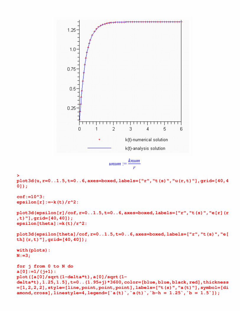
unum := knumr

> plot3d(u,r=0..1.5,t=0..6,axes=boxed,labels=["r","t(s)","u(r,t)"],grid=[40,40]); cof:=10^3: epsilon[r]:=-k(t)/r^2: plot3d(epsilon[r]/cof,r=0..1.5,t=0..6,axes=boxed,labels=["r","t(s)","e[r](r,t)"],grid=[40,40]); epsilon[theta]:=k(t)/r^2: plot3d(epsilon[theta]/cof,r=0..1.5,t=0..6,axes=boxed,labels=["r","t(s)","e[th](r,t)"],grid=[40,40]); with(plots): N:=3; for j from 0 to N do a[0]:=1/(j+1): plot([a[0]/sqrt(1-delta*t),a[0]/sqrt(1-delta*t),1.25,1.5],t=0..(1.95+j)*3600,color=[blue,blue,black,red],thickness=[1,2,2,2],style=[line,point,point,point],labels=["t(s)","a(t)"],symbol=[diamond,cross],linestyle=4,legend=[`a(t)`,`a(t)`,`b-h = 1.25`,`b = 1.5`]);

od;

N := 3

a0 := 1

a0 := 12

a0 := 13

a0 := 14

TRANHONGCO

Approved

>

> func_bankinhtrong(50, 5.2, 2, 7, Hh);

REFERENCES

[1] ю.н. РАБОТНОВ , Пoлзyчесть элементов конструкций , издательство �наука� , MOCKBA 1966[2] Lee E .H ., Radok J.R.M., Woodward W.B., Stress Analysis for Linear Viscoelastic Materials , Trans. Soc. Rheol., 3, 41-59 (1959) Disclaimer: While every effort has been made to validate the solutions in this worksheet, the author is not responsible for any errors contained and are not liable for any damages resulting from the use of this material. Legal Notice: The copyright for this application is owned by the author(s). Neither Maplesoft nor the author are responsible for any errors contained within and are not liable for any damages resulting from the use of this material. This application is intended for non-commercial, non-profit use only. Contact the author for permission if you wish to use this application in for-profit activities.