Center for Financial Studies Goethe-Universität Frankfurt House of Finance

Grüneburgplatz 1 60323 Frankfurt Deutschland

Telefon: +49 (0)69 798-30050 Fax: +49 (0)69 798-30077 http://www.ifk-cfs.de E-Mail: info@ifk-cfs.de

No. 2011/01

Long-run Growth Expectations and "Global Imbalances"

Mathias Hoffmann, Michael U. Krause, and Thomas Laubach

Center for Financial Studies Goethe-Universität House of Finance

Grüneburgplatz 1 60323 Frankfurt am Main Deutschland

Telefon: +49 (0)69 798-30050 Fax: +49 (0)69 798-30077 http://www.ifk-cfs.de E-Mail: info@ifk-cfs.de

Center for Financial Studies

The Center for Financial Studies is a nonprofit research organization, supported by an association of more than 120 banks, insurance companies, industrial corporations and public institutions. Established in 1968 and closely affiliated with the University of Frankfurt, it provides a strong link between the financial community and academia.

The CFS Working Paper Series presents the result of scientific research on selected topics in the field of money, banking and finance. The authors were either participants in the Center´s Research Fellow Program or members of one of the Center´s Research Projects.

If you would like to know more about the Center for Financial Studies, please let us know of your interest.

Prof. Michalis Haliassos, Ph.D. Prof. Dr. Jan Pieter Krahnen Prof. Dr. Uwe Walz

* We thank Toni Braun, Dale Henderson, Heinz Herrmann, Robert Kollmann, Eric Leeper, Wolfgang Lemke, Thomas Lubik, Enrique Mendoza, Gernot Müller, Lars Svensson, Mathias Trabandt, Alexander Wolman, and participants of the Bundesbank Workshop on Global Imbalances and the Crisis, the Bundesbank Spring Conference 2010, the SCE/CEF 2010 conference in London, and seminar participants at the Sveriges Riksbank, the Federal Reserve Bank of Richmond, and at the universities of Würzburg, Bonn, Münster, and Giessen for useful comments and discussions. Laubach gratefully acknowledges the hospitality and financial support of the Bundesbank. The views expressed in this paper do not necessarily reflect those of the Deutsche Bundesbank or its staff.

1 Deutsche Bundesbank, Wilhelm-Epstein-Str. 14, 60431 Frankfurt, Germany. 2 Deutsche Bundesbank, Wilhelm-Epstein-Str. 14, 60431 Frankfurt, Germany. 3 Goethe University Frankfurt and Deutsche Bundesbank. Address: Goethe University Frankfurt, Chair of Macroeconomics, House of

Finance, Grüneburgplatz 1, 60323 Frankfurt, Germany.

CFS Working Paper No. 2011/01

Long-run Growth Expectations

and "Global Imbalances"*

Mathias Hoffmann1, Michael U. Krause2, and Thomas Laubach3

January 5, 2011

Abstract This paper examines to what extent the build-up of "global imbalances" since the mid-1990s can be explained in a purely real open-economy DSGE model in which agents’ perceptions of long-run growth are based on filtering observed changes in productivity. We show that long-run growth estimates based on filtering U.S. productivity data comove strongly with long-horizon survey expectations. By simulating the model in which agents filter data on U.S. productivity growth, we closely match the U.S. current account evolution. Moreover, with household preferences that control the wealth effect on labor supply, we can generate output movements in line with the data. JEL Classification: E13, E32, D83, O40 Keywords: Open Economy DSGE Models, Trend Growth, Kalman Filter, Real-time Data,

News and Business Cycles

Axiom 1 The fundamental things apply / As time goes by - Casablanca (1942)

1 Introduction

The global economic crisis of 2008 and 2009 that began with �nancial market problems

in the United States is often seen as related to the global imbalances building up in the

preceding decade. That is, seemingly excessive borrowing by the United States in an en-

vironment of low world interest rates is seen as the pathological cause of an ever-widening

and unsustainable U.S. current account de�cit that was bound to be corrected sooner or

later. While a correction was often believed to be triggered by a large depreciation of the

dollar, the current account began to reverse itself without large exchange rate movements

(yet).1 Instead, restrictions in lending to U.S. households due to �nancial market problems

and the ensuing increase in the U.S. savings rate appear to have initiated an end to the

ever-expanding current account de�cit.

In this paper, by contrast, we propose an equilibrium explanation of the U.S. current

account � and thus also of global imbalances and their reversal � which abstracts from

�nancial factors. In particular, we show that the evolution of the U.S. current account

de�cit from 1995 onward can to a large extent be explained by households�and �rms�optimal

responses to changing long-run U.S. growth expectations and to the decline of world real

interest rates after 2000. The central role of growth expectations for our results is of course

the implication of the intertemporal approach to the current account, according to which

savings and investment decisions by forward-looking agents are based on the present value of

future incomes, relative to prevailing borrowing costs determined in world capital markets.

The basis of our explanation of U.S. current account dynamics is a standard open-

economy real stochastic growth model with capital accumulation and international trade

in real bonds and goods. Since future long-run growth is intrinsically uncertain, we assume

that the growth rate of productivity consists of persistent and transitory stochastic com-

ponents. While changes in the latter have only minor implications for the present value of

income, even small changes in the former can potentially cause major revisions of perceived

1See Obstfeld and Rogo¤ (2007) and Cooper (2008), and Feldstein (2008).

1

wealth, and thus of the commensurate consumption choices. However, the uncertain nature

of future productivity growth also requires that a signal extraction problem be solved to infer

changes in trend growth. We assume that agents use the Kalman �lter to generate long-

run productivity growth expectations from real-time U.S. productivity data and show that

these model-based productivity growth expectations are consistent with published growth

expectations from surveys.

We �nd that simulating our calibrated model with data on U.S. productivity growth

and real interest rates in the rest of the world as driving processes is su¢ cient to closely

track the actual evolution of the U.S. current account since 1995. Given that our benchmark

choice of parameter values is quite standard, this result is rather striking. Neither changing

productivity growth expectations nor interest rates alone can fully explain the data. Holding

growth expectations �xed, lower world interest rates since the late 1990s have played a role,

but they can at best explain about a �fth of the widening U.S. current account de�cit, and

cannot account for the partial reversal after the crisis of 2008/2009. This instead is accounted

for by the drop in perceived U.S. productivity growth since about 2006. We conclude that

the main driver of the U.S. current account, and thus of global imbalances, are changing

U.S. productivity growth expectations.2

The main implication of our results is that a large part of the evolution of the U.S.

current account should be seen as the e¢ cient response to changing but imperfectly observed

fundamentals. Therefore, the buildup of the current account need not be largely the result

of economic policies, such as a loose monetary stance in the U.S. along with credit market

distortions, as argued by Obstfeld and Rogo¤ (2010). Similarly, most of the reversal of the

current account since 2006 need not be the consequence of a crisis caused by �nancial turmoil.

Instead, as U.S. growth prospects have worsened, expected income streams have fallen, which

must lead to revisions of consumption and investment plans by �rms, manifesting themselves

in the current account.3 From this perspective, global imbalances need not be judged as some

2We do discuss later the extent to which changing growth expectations in the rest of the world may havecontributed to the fall in world interest rates.

3Of course, disappointed growth expectations may be at the core of the collapse of the housing market,which in turn have fed back onto the �nancial system. But the housing market developments are just oneaspect of more fundamental factors at work.

2

form of pathological disequilibrium. However, as we show, even fundamentally justi�ed

changes in actual and perceived growth can have strong e¤ects on the asset valuation of the

productive capacity of the economy, and, furthermore, can also feature concomitant output

movements in the direction we observed since 2008.

The second implication relates to the idea of a savings glut (Bernanke, 2005), according

to which a lack of investment and high savings in the rest of the world caused an excessive

supply of funds to the U.S.4 In the work of Caballero, Fahri, and Gourinchas (2008), the

superior quality and depth of the U.S. �nancial system have led global investors to supply

funds cheaply to the U.S., while Mendoza, Quadrini, and Rios-Rull (2009) explain global

imbalances as a consequence of asymmetric degree of �nancial development. The current

account reversal in the wake of the crisis would then be explained by the interaction of

�nancial frictions and portfolio rebalancing of international investors. While these factors

certainly have played an important role, the fact that we control for the associated interest

rate movements suggests that more is needed for a complete account of the global imbalances

of the 2000s.

Our reasoning is closely related to the analysis of emerging market current account crises

of Aguiar and Gopinath (2008), who �nd that shocks to trend productivity growth can be

a major source of �uctuations in emerging markets. The authors use a small open economy

model to identify the true growth trends from current account and consumption data, by as-

suming that households perfectly observe changes to the long-run growth trend. The growth

trend thus inferred is highly volatile.5 In contrast, we take into account that changes in

the growth trend are only perceived with noise, and constrain ourselves to consider changes

in productivity growth expectations that are consistent with measured expectations from

surveys, such as the Survey of Professional Forecasters. We thus show that changes in per-

ceived long-run productivity growth imply current account movements even for a developed

economy as the U.S., and also are able to match such movements in a quantitatively more

plausible manner.

4Note that U.S. interest rates have not been systematically lower than in other developed economies.See Gruber and Kamin (2009), and further evidence presented below.

5Boz et al. (2010) employ a similar model with learning and show that it matches emerging marketdynamics better than under the full information assumption of Aguiar and Gopinath (2008).

3

Once we acknowledge that long-run growth rates cannot be known with certainty, while

at the same time being central to consumption and savings decisions, we see that revisions

to growth expectations must be perpetually triggering changes in economic choices. This

is akin to the notion of news-driven business cyles, as introduced by Beaudry and Portier

(2004) and others.6 In fact, the news on future productivity inherent in the updates of long-

run growth generated by the Kalman Filter on current productivity amount to what Walker

and Leeper (2011) label �correlated news.�These authors show that this type of information

�ow produces empirically more plausible impulse responses than the �i.i.d. news�typically

analysed. The household preferences that we assume are often used in the news literature,

as they allow to control the wealth e¤ect on labor supply. Under a parameterization based

on the estimate by Schmitt-Grohe and Uribe (2008), our historical simulations do indeed

feature a drop in U.S. output by 2009. Note, however, that our explanation of current

account movements also prevails for standard preferences with wealth e¤ects, because the

present value theory of the current account is one of consumption relative to income, and

not of the level of income.

A large literature has explored the intertemporal approach to the current account (aka

the present value model). The contrast between our ability to match the U.S. current account

and the less conclusive �ndings in previous work lies in our treatment of interest rates and

productivity. In their comprehensive survey, Nason and Rogers (2006) report di¢ culties in

matching the data with that approach. However, all these tests assume a �xed world interest

rate for the (small) countries under consideration, and a process in productivity that is trend

stationary, rather than di¤erence stationary. In other words, shocks to the trend growth

rate are not considered. Neither productivity level shocks nor shocks to demography and

government spending among others can explain the current account via the present value

mechanism. From the perspective of our results, this is not surprising, since only changes

in growth rates have su¢ ciently large e¤ects on present values and therefore the current

account. Other important papers studying the current account and its relation to growth

6This stimulated a rapidly growing literature on news �shocks�. See, for example, Jaimovich and Rebelo(2009), Schmitt-Grohé and Uribe (2008), and Fujiwara, Hirose, and Shintani (2008). Boz, Daude, and Durdu(2010) note the general link between news and information updates in their work on emerging market currentaccounts. We make this link explicit in section 5.

4

take a long-run perspective over many decades, and assume that agents have perfect foresight

and/or perfect information about future growth.7

The paper proceeds from here as follows. First, in section 2, we motivate our analysis

by showing the evolution of global long-run growth expectations and real long-term interest

rates. These data suggest a close link between U.S. long-run growth expectations and the U.S.

current account, but a breakdown of the close relationship between growth expectations and

interest rates in the rest of the world in the early 2000s. In section 3, we develop our model

�a two-country real open economy stochastic growth model �that incorporates changes in

long-run trend growth. We also introduce the signal-extraction problem of inferring long-

run from short-run productivity movements, and its solution by means of the Kalman �lter.

Calibration and simulation results are presented in section 4, where we �rst illustrate the

economics of the model using impulse responses. Then we simulate the model using data

on U.S. productivity growth and rest-of-the-world real interest rates, and on as the input to

the Kalman �lter. In section 5 we examine the robustness of our results with respect to a

di¤erent productivity process. Furthermore, we discuss formally the nature of information

shocks �or, news � in our model, and argue that shocks to long-run growth trends are a

plausible and concrete example where news drive behavior. Section 6 o¤ers conclusions and

directions for future research.

2 The evolution of long-run growth expectations andworld interest rates

The main explanation for the emergence of �global imbalances� that we emphasize is the

evolution of perceived trend growth rates in the U.S. relative to world borrowing conditions.

In this section, we aim to highlight some broad features of the data. The �rst step is to show

how output growth expectations in the U.S. and in a group of major countries, chosen to

represent the rest of the world, evolve. The appropriate source of choice here are the surveys

of long-run outcome growth expectations as compiled by Consensus Economics. Note that,

7These papers include Engel and Rogers (2006), Ferrero (2010), and Chen, Imrohoroglu, and Imrohoroglu(2009).

5

while these data are suggestive for our purposes, they are not operational in the simulations

of the model, since output growth is an endogenous outcome of a variety of factors, in

particular productivity growth.8

Since 1989, Consensus Economics conducts a monthly survey of professional economists.

For the major industrialized economies, every six months this survey has included questions

about participants� expectations of real GDP growth and other macroeconomic variables

at horizons up to ten years. For the major economies of the Asia-Paci�c region these long-

horizon expectations start in 1995. We focus on real GDP growth expectations at the longest

horizon (6 to 10 years ahead) for the U.S. and a set of nine countries that in 2008 jointly

accounted for about 2/3 of world GDP. Moreover, the nine countries accounted in 2003 for

about 2/3 of U.S. imports and slightly less of U.S. exports.9

1994 1996 1998 2000 2002 2004 2006 2008 2010 20122

2.5

3

3.5

4

4.5

5Forecasts of real GDP growth 6­10 years ahead

USRest­of­world (9)

1994 1996 1998 2000 2002 2004 2006 2008 2010 2012­2.5

­2

­1.5

­1

­0.5Trend growth expectations: US minus Rest­of­World

Figure 1: Consensus forecasts of real GDP growth 6-10 years ahead

8In section 3.3 we compute estimates of trend labor productivity growth and compare these to long-horizonexpectations of labor productivity growth from the Survey of Professional Forecasters (SPF). We use theconsensus forecasts here to emphasize the international dimension of changes in perceive trend growth, butuse the SPF below because only the latter provides long-horizon estimates of labor productivity growth.

9The countries included are the U.S., Japan, Germany, France, the U.K., Italy, Canada, China, Koreaand Taiwan. The shares in world GDP are taken from www.ers.usda.gov, the shares in U.S. imports andexports from Loretan (2005).

6

The top panel of Figure 1 shows these expectations for the U.S. and the GDP-weighted

average of the expectations for the other nine countries (henceforth referred to as the �rest

of the world�).10 The bottom panel of Figure 1 shows the di¤erence between the trend

growth expectations for the US and the weighted average growth expectations for our �rest-

of-world�aggregate. As can be seen, participants�perceptions of U.S. trend growth relative

to the �rest of the world�rose by about 1.5 percentage points between 1998 and 2003, then

remained roughly at that level until about 2005, and has since retracted about 1 percentage

point. While the initial increase re�ected in roughly equal measure an increase in perceived

U.S. trend growth and a decline in trend growth elsewhere, the reversal in recent years is

mostly due to lower U.S. trend growth expectations.

1995 2000 2005 2010­7

­6

­5

­4

­3

­2

­1

0US NX/GDPRoW­US expected growth (scaled)

Figure 2: Consensus Forecast Growth Expectations and the Current Account

Figure 2 provides ocular evidence on the link between the current account and growth

expectations, which motivates our analysis below. The points marked with x depicts the gap

betwen U.S. and world growth expectations from Consensus Forecasts as shown in Figure 1.

The blue line is the U.S. current account relative to GDP since 1995. It is striking to us how

10The long-horizon forecasts are always published in April and October, and are shown in the �gure inthe �rst and third quarter of each year.

7

1994 1996 1998 2000 2002 2004 2006 2008 2010 2012­1

0

1

2

3

4

5Long­term real rates

USRest­of ­world (6)

1994 1996 1998 2000 2002 2004 2006 2008 2010 20120

2

4

6Long­term real rates and trend growth expectations: Rest­of ­World

1994 1996 1998 2000 2002 2004 2006 2008 2010 20123.5

4

4.5

5RoW real rate (lef t scale)RoW growth expectations (right scale)

Figure 3: Long-term real rates and growth expectations

the growth expectations di¤erential leads the evolution of the current account. Our model

simulations based on U.S. productivity growth expectations and world interest rates below

will exhibit this pattern even more strongly.

The �nal point of this section concerns the link between world real interest rates and

growth expectations. The upper panel of Figure 3 shows estimates of the ex-ante long-term

real government bond yields for the U.S. and a subset of six countries of our nine-country

�rest-of-world�aggregate.11 The lower panel plots the real long-term interest rate in the rest

of the world (against the left axis) and the weighted growth expectations in the rest of the

world. As can be seen, until about 2003 these two series moved remarkably closely together.

Since then, however, there is a widening gap suggesting that other factors than perceived

trend growth contributed signi�cantly to the movement of the world real interest rate.

Potential explanations for this widening gap, other than growth expectations, have fo-

11For each country, long-horizon in�ation expectations are proxied by a slow-moving partial-adjustmentequation ��et = ���et�1 + (1 � �)�t using CPI in�ation. This type of equation does a good job proxyinglong-horizon in�ation expectations in the U.S. We exclude China and Taiwan from the computation of the�rest-of-world� real interest rate for lack of government bond yield data, and Korea because of the stronge¤ects of the Asian crisis on its yields.

8

cused on the relative inability of the rest of the world to create the safe assets they demand

(Caballero et al., 2008), or increasing purchases of U.S. government issued paper by China,

which is di¢ cult to model. However, what matters for U.S. households and �rms are borrow-

ing conditions, not the speci�c factors that explain their evolution. Therefore, we directly

include the realized path of the world real interest rate in our simulations rather than backing

out the particular factors that generated it.

3 The Model

In this section we develop our real stochastic growth model of open economies. While most

elements are standard from the open-economy real business cycle literature, there are two

key modi�cations: learning about the rate of productivity growth, and generalized household

preferences that allow for various strength of the wealth e¤ect on labor supply in response

to changes in perceived productivity growth.

3.1 Setup

The model consists of two countries, home and foreign (the rest of the world), which is

denoted by an asterisk �. We normalize the population size of the domestic economy to

1 and the relative population size of the foreign economy, i.e., rest of the world, to P�, so

that 1=(1+P�) is the fraction of home population in the world. Each country is inhabited by

a large number of in�nitely living households and endowed with a constant returns to scale

production technology utilized by competitive �rms. Firms produce a single good which can

be used for consumption and investment in both countries. For ease of exposition, we fully

consider only the domestic economy. The foreign country is identical in terms of preferences

and technology.

Households in the home economy maximize the present value of their instantaneous

utility, discounted with a factor �: Thus a representative households maximizes

E0

1Xt=0

�t��Ct � h �Ct�1

�� �L1+�t Xt

�1�� � 11� � ;

where Xt =�Ct � h �Ct�1

� X1� t�1

�ZtZt�1

�1� . Utility depends on consumption Ct relative to

9

a weighted external habit stock �Ct�1, given by past aggregate consumption, and a weighted

disutility of labor, Lt. The weighting factor Xt governs the extent of the wealth e¤ect on

labor supply, and is inspired by Jaimovich and Rebelo (2009). The parameter is between

zero and one. When = 0; these simplify to Greenwood, Hercowitz, and Hu¤mann (1988)

preferences, often used in the open economy literature, allowing plausible labor responses

to positive wealth innovations. When = 1; the preferences are the growth consistent

preferences from King, Plosser, and Rebelo (1988). In contrast to Jaimovich and Rebelo,

we extend the model by including the scale factor�

ZtZt�1

�1� ; to ensure that the model is

consistent with steady state growth in aggregate labor-augmenting technology Zt, de�ned

below.12 Note that the expectations operator denotes here the expectation conditional on

information available in the current period, which may be imperfect.

The household faces two constraints, the budget constraint and the capital accumulation

equation. The former is given by

WtLt + rktKt�1 + rt�1Bt�1 = Ct + It +Bt �Bt�1:

Income consists of real labor income WtLt; as well as return on capital determined in the

previous period, rktKt�1, and the net return on a single non-contingent real bonds, rt�1Bt�1,

respectively. The income is used to �nance consumption Ct, investment It, and to accumulate

net foreign assets, Bt. When agents borrow from the rest of the world it follows that Bt <

0. Financial markets are incomplete in that households cannot insure against all possible

contingencies. The capital accumulation constraint equals

Kt = (1� �)Kt�1 + It

"1� �

2

�ItIt�1

� eg�2#

:

Investment is subject to quadratic adjustment costs, with �(1) = 0; �0(1) = 0; and �00(1) > 0

at the stationary steady state and g the long-run net growth rate. When agents take net

positions in international bond markets, a �nancial intermediation premium must be paid,

which relates the domestic interest rate rt and the rest of the world�s real interest rate r�t by

the following function:12Jaimovich and Rebelo (1998) impose that > 0; so that preferences are growth consistent, by the

weight on the King-Plosser-Rebelo part of preference. Very low values of imply however in the limit highlypersistent deviations from the steady state growth part.

10

rt = r�t � '

�exp

�BtYt� BY

�� 1�; (1)

where B=Y re�ects the steady-state ratio of the country�s net foreign assets to GDP.13 Thus,

both the actual net foreign asset position relative to GDP, Bt=Yt, and movements of the real

interest rate r�t in the rest of the world will a¤ect the borrowing conditions of the domestic

economy.

A competitive representative �rm in the domestic economy produces a single good ac-

cording to the technology

Yt = eK�t (ZtLt)

1�� ;

where 0 < � < 1, and eKt is the capital stock used by the �rm. In equilibrium it will have to

equal the capital Kt�1 supplied by households. Aggregate technology evolves according to

lnZt � lnZt�1 = gt + !t; (2)

with

gt =�1� �g

�g + �ggt�1 + �t: (3)

Both !t and vt are i.i.d. distributed as �t � N (0; �2v) and !t � N (0; �2!). The growth

in technology thus has two components. An innovation !t leads to a permanent shift in

the level of technology Zt, but has no persistent e¤ects on the growth rate of technology,

ln (Zt=Zt�1). An innovation vt, by contrast, leads to a sequence of changes in Zt in the same

direction because it raises its growth rate temporarily above its steady-state growth rate:14

The foreign economy (i.e., the rest of the world) is identically speci�ed. In particular,

we assume that it faces the same steady-state growth rate. Nonetheless, both regions can

grow at di¤erent rates for a substantial amount of time, depending on the realizations of the

domestic and foreign technology shocks. Since the model is expressed in per capita terms,

the global goods market clearing condition takes account of the relative sizes of the two

13The �nancial intermediation premium ensures that the net foreign asset position becomes stationary inthe linearized version of the model (see Schmitt-Grohe and Uribe, 2003).

14An alternative formulation of the technology process involving regime switching has been explored inKahn and Rich (2007).

11

regions:C�t P�1 + P� +

Ct1 + P� +

I�t P�1 + P� +

It1 + P� =

Y �t P�1 + P� +

Yt1 + P� : (4)

For later expositional purposes, the world real interest rate can also be written as the average

of the foreign and domestic interest rates.

rwt = r�t

P�1 + P� + rt

1

1 + P� : (5)

Finally, bond market clearing requires that

B�tP�1 + P� +

Bt1 + P� = 0; (6)

since bonds are in zero net supply in the world economy.

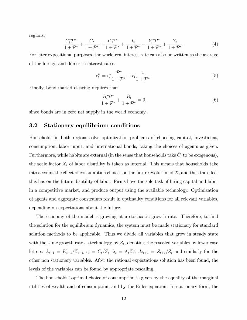
3.2 Stationary equilibrium conditions

Households in both regions solve optimization problems of choosing capital, investment,

consumption, labor input, and international bonds, taking the choices of agents as given.

Furthermore, while habits are external (in the sense that households take �Ct to be exogenous),

the scale factor Xt of labor disutility is taken as internal. This means that households take

into account the e¤ect of consumption choices on the future evolution ofXt and thus the e¤ect

this has on the future disutility of labor. Firms have the sole task of hiring capital and labor

in a competitive market, and produce output using the available technology. Optimization

of agents and aggregate constraints result in optimality conditions for all relevant variables,

depending on expectations about the future.

The economy of the model is growing at a stochastic growth rate. Therefore, to �nd

the solution for the equilibrium dynamics, the system must be made stationary for standard

solution methods to be applicable. Thus we divide all variables that grow in steady state

with the same growth rate as technology by Zt; denoting the rescaled variables by lower case

letters: kt�1 = Kt�1=Zt�1; ct = Ct=Zt; �t = �tZ�t ; dzt+1 = Zt+1=Zt and similarly for the

other non stationary variables. After the rational expectations solution has been found, the

levels of the variables can be found by appropriate rescaling.

The households�optimal choice of consumption is given by the equality of the marginal

utilities of wealth and of consumption, and by the Euler equation. In stationary form, the

12

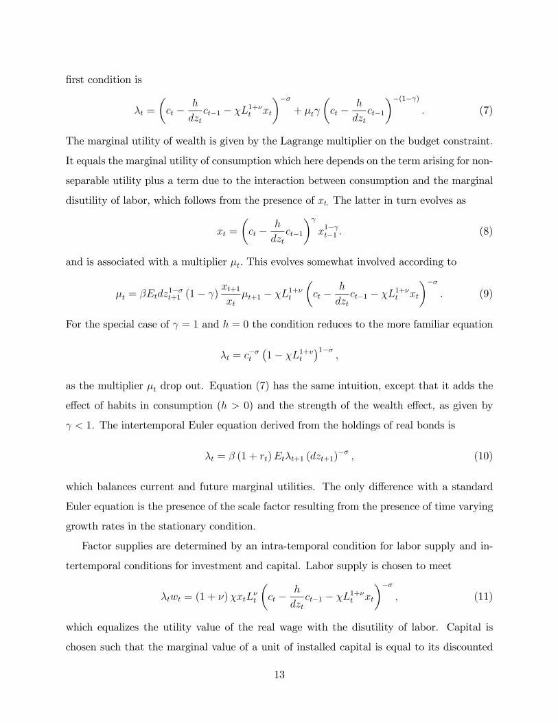
�rst condition is

�t =

�ct �

h

dztct�1 � �L1+�t xt

���+ �t

�ct �

h

dztct�1

��(1� ): (7)

The marginal utility of wealth is given by the Lagrange multiplier on the budget constraint.

It equals the marginal utility of consumption which here depends on the term arising for non-

separable utility plus a term due to the interaction between consumption and the marginal

disutility of labor, which follows from the presence of xt: The latter in turn evolves as

xt =

�ct �

h

dztct�1

� x1� t�1 : (8)

and is associated with a multiplier �t: This evolves somewhat involved according to

�t = �Etdz1��t+1 (1� )

xt+1xt�t+1 � �L1+�t

�ct �

h

dztct�1 � �L1+�t xt

���: (9)

For the special case of = 1 and h = 0 the condition reduces to the more familiar equation

�t = c��t

�1� �L1+vt

�1��;

as the multiplier �t drop out. Equation (7) has the same intuition, except that it adds the

e¤ect of habits in consumption (h > 0) and the strength of the wealth e¤ect, as given by

< 1. The intertemporal Euler equation derived from the holdings of real bonds is

�t = � (1 + rt)Et�t+1 (dzt+1)�� ; (10)

which balances current and future marginal utilities. The only di¤erence with a standard

Euler equation is the presence of the scale factor resulting from the presence of time varying

growth rates in the stationary condition.

Factor supplies are determined by an intra-temporal condition for labor supply and in-

tertemporal conditions for investment and capital. Labor supply is chosen to meet

�twt = (1 + �)�xtL�t

�ct �

h

dztct�1 � �L1+�t xt

���; (11)

which equalizes the utility value of the real wage with the disutility of labor. Capital is

chosen such that the marginal value of a unit of installed capital is equal to its discounted

13

expected value, which is the sum of the marginal product of capital and the expected value

of capital, net of depreciation. Thus capital adjusts to meet the Euler equation

Qt = Et�t+1�rkt+1 +Qt+1 (1� �)

�; (12)

where �t+1 = (dzt+1)�� �t+1=�t is the appropriately de�ned stochastic discount factor, and

rkt is the rental rate of capital and Qt the marginal value of a unit of installed capital. In

the presence of adjustment costs investments follows

1 = Qt

1� �

2

�itit�1

dzt � eg�2� itit�1

dzt�

�itit�1

dzt � eg�!

(13)

+�Et�t+1Qt+1

�it+1itdzt+1 � eg

��dzt+1

it+1it

�2;

and the stationary capital stock evolves according to

kt = (1� �)kt�1dzt

+ it

"1� �

2

�itit�1

dzt � eg�2#

: (14)

Aggregate output of �rms in the domestic economy equals

yt =

�kt�1dzt

��L1��t : (15)

The optimal choices of kt�1 and Lt are governed by the equality of marginal products to

factor prices:

wt = (1� �)�kt�1dzt

��L��t ; (16)

rkt = �

�kt�1dzt

��(1��)L1��t : (17)

Finally, from the budget constraint it follows that output equals spending plus net foreign

asset accumulation:

yt = ct + it + bt � bt�1 +dzt � (1 + rt�1)

dztbt�1: (18)

These stationary conditions together with (1)-(6) and their foreign counterparts deter-

mine the equilibrium of the system, along with the corresponding transversality conditions.

14

A rational expectations equilibrium of the model is a set of sequences fct, c�t , yt, y�t , Lt, L�t ,

it, i�t , �t, ��t , �t, �

�t , Qt, Q

�t bt, kt, k

�t , rt, r

�t , r

kt , r

k�t , wt, w

�t , xt, x

�t , dzt, dz

�t , gt, g

�t g for t � 0

given the sequences of shocks f"t, �t, "�t , ��tg1t=0. The model is solved by log-linearizing the

stationary equilibrium equations around the stationary steady state, and applying familiar

methods for the solution of rational expectations models (e.g., Sims, 2002).

3.3 Extracting the perceived trend growth rate

As in Edge, Laubach, andWilliams (2007) and Gilchrist and Saito (2008), agents only observe

the current level of technology Zt, but are unable to disentangle changes in lnZt from lnZt�1

into one-o¤ level shifts !t and persistent growth rate changes due to innovations �t; in the

notation introduced above. They therefore form at each point in time a best estimate gtjt

of the current level of trend growth. Given the linearity of our setup, this best estimate is

obtained by the Kalman �lter according to the recursion

gtjt = (1� �)�ggt�1jt�1 + � ln dzt;

where dzt = Zt=Zt�1. The Kalman gain � is given by

� =� � (1� �2g) + �

q((1� �2g)=�)2 + 1 + 2(1 + �2g)=�

2 + � � (1� �2g) + �q((1� �2g)=�)2 + 1 + 2(1 + �2g)=�

;

where the signal-to-noise ratio � � �2�=�2! measures the importance of innovations to trend

growth relative to permanent one-o¤ changes to the level of technology. All agents, domestic

and foreign, share the same signal extraction problem for the productivity process.

The results of our analysis rely critically on the gain parameter �, which gives the degree

to which agents update their estimate of trend growth based on actual productivity growth.

To calibrate the gain, we use the median unbiased estimator of the signal-to-noise ratio of

Stock and Watson (1998). Applying this method to quarterly labor productivity data for

the U.S. nonfarm business sector from 1948Q1 to 2008Q4 leads to an estimated signal-to-

noise ratio, � of 0.025. Because the Stock-Watson estimator is based on the assumption of

a unit root growth rate process, this implies a quarterly gain of 0.025 as well. In our model

calibration, for the sake of stationarity of the model, we assume that �g is close to, but

15

1995 2000 2005 20101

1.2

1.4

1.6

1.8

2

2.2

2.4

2.6

2.8Kalman filter using real­time dataKalman filter using revised dataSPF Median ForecastSPF Mean Forecast

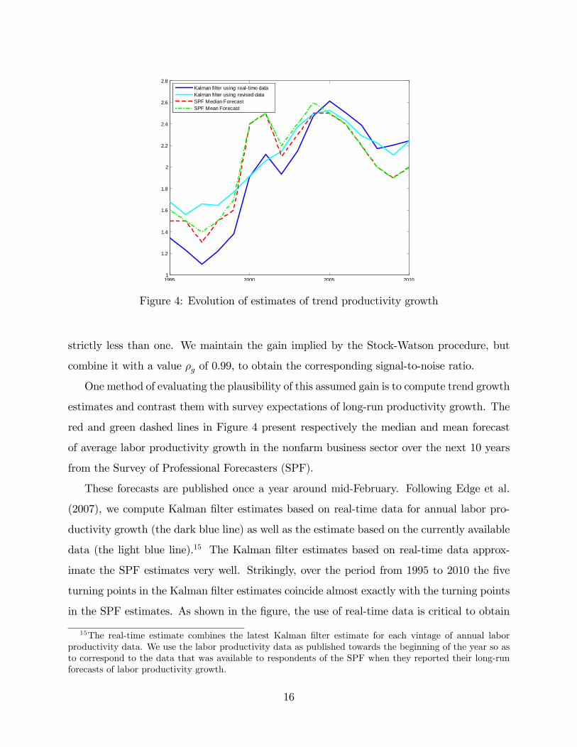
Figure 4: Evolution of estimates of trend productivity growth

strictly less than one. We maintain the gain implied by the Stock-Watson procedure, but

combine it with a value �g of 0.99, to obtain the corresponding signal-to-noise ratio.

One method of evaluating the plausibility of this assumed gain is to compute trend growth

estimates and contrast them with survey expectations of long-run productivity growth. The

red and green dashed lines in Figure 4 present respectively the median and mean forecast

of average labor productivity growth in the nonfarm business sector over the next 10 years

from the Survey of Professional Forecasters (SPF).

These forecasts are published once a year around mid-February. Following Edge et al.

(2007), we compute Kalman �lter estimates based on real-time data for annual labor pro-

ductivity growth (the dark blue line) as well as the estimate based on the currently available

data (the light blue line).15 The Kalman �lter estimates based on real-time data approx-

imate the SPF estimates very well. Strikingly, over the period from 1995 to 2010 the �ve

turning points in the Kalman �lter estimates coincide almost exactly with the turning points

in the SPF estimates. As shown in the �gure, the use of real-time data is critical to obtain

15The real-time estimate combines the latest Kalman �lter estimate for each vintage of annual laborproductivity data. We use the labor productivity data as published towards the beginning of the year so asto correspond to the data that was available to respondents of the SPF when they reported their long-runforecasts of labor productivity growth.

16

0 20 40 60 800

0.1

0.2

0.3

0.4

0.5

0.6

0.7

0.8

0.9

1

Quarters

Productivity growth: Growth rate shock to technology

full info.imp. info.

0 20 40 60 800

0.1

0.2

0.3

0.4

0.5

0.6

0.7

0.8

0.9

1

Quarters

Productivity growth: Level shock to technology

full info.imp. info.

Figure 5: Growth expectations relative to fundamentals

this result: The Kalman �lter estimate based on the revised data is not nearly as successful

in reproducing the patterns of the SPF estimates. The conclusion that we draw from this

�gure is that our simple learning model, with the gain calibrated from the Stock-Watson

median unbiased estimator, provides a plausible model for the formation of trend growth

expectations.

How growth expectations evolve relative to fundamentals is illustrated in Figure 5, where

we simulate a one standard deviation shock to the growth rate in the upper panel of the

�gure. This results in the blue line, which also depicts the case of full information. The

growth rate of technology jumps up and with persistence �g slowly returns to the long-run

steady state growth rate. Under imperfect information, and the estimated Kalman gain,

agents assign only 2.5 percent of a productivity innovation to the permanent change in the

growth rate rather than merely the level. Subsequently, as technology growth is persistently

higher than expected, the Kalman �lter updates the perceived growth rate. Note that the

gap between the blue and red-dashed line is equal to the perceived transitory shock, whose

role diminishes over time.

17

In the lower panel of Figure 5, we see the corresponding evolution of the growth rate of

productivity after a one time shock to the level. Again, the Kalman �lter assigns 2.5 percent

of the change to the growth rate shock, and the remainder to the transitory shock. However,

even though there are no further changes to technology, the long-term growth expectations

continue to be above steady state, since they are revised only slowly downwards.

3.4 Calibrating the remainder of the model

In our calibration, we assign values to the deep parameters using guidance from the literature

and a priori reasoning. Their values are displayed in Table 1.

International capital mobility is high, in that we set the international risk premium

parameter to a value of ' = 0:0002; since we consider a long-run horizon, and a period where

�nancial market appear highly integrated. For simplicity we assume that in the steady state

B = B� = 0. The size of the domestic economy in the world economy is assumed to be 25%

so that P� equals 3.

Household preferences are calibrated based on values from Schmitt-Grohe and Uribe

(2008), who estimate the Jaimovich-Rebelo (2008) model of news shocks. They �nd a value

for the coe¢ cient of relative risk aversion close to � = 2 and a labor supply parameter of

about � = 1; which implies a Frisch labor supply elasticity of 1. In line with Schmitt-Grohe

and Uribe we set the steady state hours worked L = 0:2. Most crucially, the parameter

determining the response of labor supply to changes in consumption, is set based on the

estimation of Schmitt-Grohe and Uribe, at = 0:0075: This is somewhat higher than the

value of Jaimovich and Rebelo, who set = 0:0001: Both values imply that the positive e¤ect

of increased consumption on labor supply only slowly fades away. For < 1, the marginal

disutility of labor will rise as much with consumption, since Xt will grow slower than the

stock of consumption, Ct � hCt�1, so that Xt= (Ct � hCt�1) initially falls. The implication

of this is that current labor supply may rise after increased perceived wealth. Thus, as

falls the wealth elasticity of labor supply declines. We also follow Schmitt-Grohe and Uribe

estimates and set the habit formation in consumption h = 0:85. This value is in line with

other estimates of habit formation in the literature, e.g. Smets and Wouters (2007). The

18

discount factor � is set at a quarterly value of 0:9975.

Table 1: Parameters of the modelParameters Values

' International risk premium 0:0002� Coe¢ cient of relative risk aversion 2� Labor supply parameter 1L Steady state hours worked 0:2 Wealth elasticity of labor supply 0:0075h Habit formation in consumption 0:85� Discount factor 0:9975� Capital share 0:3� Depreciation rate 0:025� Investment adjustment costs 5P� Size of the foreign economy 3

In terms of technology, the parameter of the production function is set at � = 1=3: Capital

depreciates at quarterly rate � = 0:025: The investment adjustment costs are calibrated at

� = 5; which is in line with the literature (e.g., Smets and Wouters, 2003). The foreign

country has identical preferences and technologies. All these parameter values determine

the steady state of the stationary version of the model. For the simulations, we rescale the

endogenous variables either to actual levels or to growth rates, to match them with actual

data.

4 Simulating trend growth expectations and the U.S.current account

In this section we use the calibrated model to quantitatively explore the link between growth

expectations and the U.S. current account. We focus on four variables, the current account,

the present value of income as generated by the model, output, and the rest-of-the-world real

interest rate. First, we show the impulse responses of these variables to one-time one percent

shocks to the growth rate of productivity, where we use the properties of the productivity

process and the associated Kalman gain. Second, we conduct a full historical simulation of

the U.S. current account by feeding the data for U.S. labor productivity and the rest-of-the-

world real interest rate into the solution of the model.

19

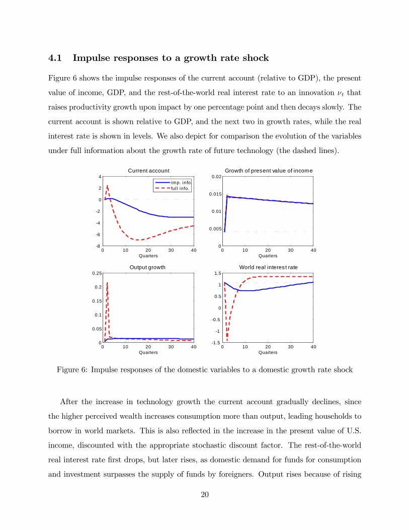
4.1 Impulse responses to a growth rate shock

Figure 6 shows the impulse responses of the current account (relative to GDP), the present

value of income, GDP, and the rest-of-the-world real interest rate to an innovation �t that

raises productivity growth upon impact by one percentage point and then decays slowly. The

current account is shown relative to GDP, and the next two in growth rates, while the real

interest rate is shown in levels. We also depict for comparison the evolution of the variables

under full information about the growth rate of future technology (the dashed lines).

0 10 20 30 40­8

­6

­4

­2

0

2

4

Quarters

Current account

imp. info.ful l info.

0 10 20 30 400

0.005

0.01

0.015

0.02Growth of present value of income

Quarters

0 10 20 30 400

0.05

0.1

0.15

0.2

0.25Output growth

Quarters0 10 20 30 40

­1.5

­1

­0.5

0

0.5

1

1.5World real interest rate

Quarters

Figure 6: Impulse responses of the domestic variables to a domestic growth rate shock

After the increase in technology growth the current account gradually declines, since

the higher perceived wealth increases consumption more than output, leading households to

borrow in world markets. This is also re�ected in the increase in the present value of U.S.

income, discounted with the appropriate stochastic discount factor. The rest-of-the-world

real interest rate �rst drops, but later rises, as domestic demand for funds for consumption

and investment surpasses the supply of funds by foreigners. Output rises because of rising

20

labor supply.

The impulse response show clearly the di¤erence between the imperfect and full informa-

tion case. Without the slow dissemination of knowledge about the growth trend, all variables

react more pronounced and partly less persistent. The current account de�cit builds up faster

because the higher perception of long-run growth, and thus of wealth leads households to

increase consumption faster. Also, investment demand is higher because agents aim at build-

ing up the capital stock faster to exploit the higher marginal product of capital. The reason

that output rises is again the increase in labor supply, due to the mitigated wealth e¤ect

discussed later. Under our parameterization, = 0:0075; based on Schmitt-Grohé and Uribe

(2008), the e¤ect of higher expected future wealth on labor supply is enormous.

We now turn to the historical simulation of these variables. In a later section, we dig

deeper into the reasons for the behavior of labor supply and the role of preferences.

4.2 Historical simulation of the U.S. current account

For the historical simulation of the model we use only two real time data inputs: the produc-

tivity data from which agents infer the long-run growth trend of labor productivity, and the

proxy of the rest-of-the-world real interest rate, described in section 2, and show the implied

evolution of the U.S. current account and the other variables. This section reports the results

obtained with BLS labor productivity growth data; in the next section, we alternatively use

an estimate an estimate of TFP. Note that the historical simulation starts in 1991, a period

when the U.S. current account was virtually balanced.

As pointed out earlier, the reason for using the rest-of-the-world real interest rate rather

than a measure of rest-of-the-world growth expectations (or even rest-of-the-world productiv-

ity growth) is that the former provides a better measure of the external �nancing conditions

relevant for U.S. households� decisions. As discussed in section 2, the latter is not well

explained by rest-of-the-world income growth expectations alone.16 Rather than trying to

model a host of factors that fully explain the rest-of-the-world real interest rate, we use it as

a direct input to the simulation. The simulation thus identi�es the particular evolution of

16There is also the more technical issue that measures of productivity comparable to the U.S. data are infact not readily available for several of the countries in our rest-of-the-world aggregate.

21

the U.S. current account that is consistent both with U.S. productivity growth expectations

and the rest-of-the-world real interest rate.17

1995 2000 2005 2010­7

­6

­5

­4

­3

­2

­1

0DataModel

Figure 7: Actual and simulated evolution of the U.S. current account

Figure 7 presents the main result of this paper: the U.S. current account is to a large

extent explained by U.S. productivity growth expectations along with world borrowing con-

ditions as re�ected in the world real interest rates. The match of the two lines is quite

striking, given the rather simple structure of our basic real open-economy model. Notably,

the buildup of the current account de�cit comes to an end at about 2006, and the de�cit

closes somewhat. As will be seen below, this is solely due to smaller increases in productiv-

ity growth, which leads agents to revise income growth expectations downward. The sharp

reduction in the de�cit at the very sample end, owes presumably to the collapse of trade

�nance in the immediate aftermath of the Lehman bankruptcy, something that our model

is of course not designed to replicate.

What is the economics behind the behavior of the current account? Taking the present

value model literally, we compute the present discounted value of income as perceived by

17To present agents with a stochastic process for the world interest rate, we �t an AR(1) process to it.The estimated persistence parameter over the time period 1991:1 to 2009:4 equals 0.94.

22

agents in the model. That is, at each point in time, we use households�stochastic discount

factor to value the expected income streams, thus getting a measure of perceived wealth.

This perception of wealth is what households base their consumption (smoothing) decisions

on, and leads them to borrow if the prevailing rest-of-the-world real interest rate is below the

one that would obtain under autarky. Obviously, the buildup of the current account re�ects

the fact that rest-of-the-world real interest rates are lower than what market forces in a

closed economy would force the interest rate to be, namely the one that equalized current

consumption and investment with current output.

1995 2000 2005 201040

45

50

55

60

65

70

75

80

Figure 8: Simulated present value of income

Figure 8 shows clearly the large changes in the level of wealth that go along with changes

in perceived income growth. Interestingly, we observe only a slight downward revision of

wealth after 2000, the bursting of the dotcom bubble, followed, however, by an acceleration

in 2003 and 2004: From 2004 up until 2006 wealth perceptions stagnated at a high level,

until falling to a lower level in 2007. Most striking is the large drop in wealth towards

around 2007/2008. The revision in wealth must, by the logic of our model, lead to adjust-

ments in agents consumption and investment plans and should manifest itself also in output

movements.

23

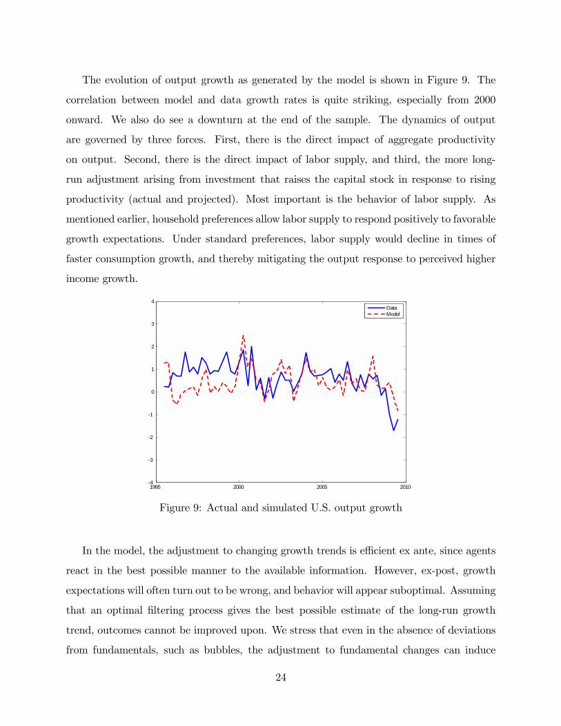
The evolution of output growth as generated by the model is shown in Figure 9. The

correlation between model and data growth rates is quite striking, especially from 2000

onward. We also do see a downturn at the end of the sample. The dynamics of output

are governed by three forces. First, there is the direct impact of aggregate productivity

on output. Second, there is the direct impact of labor supply, and third, the more long-

run adjustment arising from investment that raises the capital stock in response to rising

productivity (actual and projected). Most important is the behavior of labor supply. As

mentioned earlier, household preferences allow labor supply to respond positively to favorable

growth expectations. Under standard preferences, labor supply would decline in times of

faster consumption growth, and thereby mitigating the output response to perceived higher

income growth.

1995 2000 2005 2010­4

­3

­2

­1

0

1

2

3

4DataModel

Figure 9: Actual and simulated U.S. output growth

In the model, the adjustment to changing growth trends is e¢ cient ex ante, since agents

react in the best possible manner to the available information. However, ex-post, growth

expectations will often turn out to be wrong, and behavior will appear suboptimal. Assuming

that an optimal �ltering process gives the best possible estimate of the long-run growth

trend, outcomes cannot be improved upon. We stress that even in the absence of deviations

from fundamentals, such as bubbles, the adjustment to fundamental changes can induce

24

substantial strain on an economy. In spite of the absence of �nancial or nominal frictions,

the model is able to generate behavior of output growth that in some respects matches actual

data. For example, the model generates a downturn in output �an actual recession in terms

of negative growth rates �solely as the result of a downward revision in wealth arising from

slowing down productivity growth.

4.3 The role of trend growth and the savings glut hypothesis

In this section we assess the importance of trend growth expectations and the world real

interest rate for the US current account. It has been argued that an excessive supply of funds

to world �nancial markets, a savings glut, has resulted in a �ow of savings into the U.S., and

thus generating the large current account de�cit of the 2000s. One way to shed light on this

issue is to ask how the current account would have evolved had U.S. productivity growth

not picked up since the late 1990s. We operationalize this by keeping productivity growth

expectations constant at its long run steady-state rate over the sample, but still feeding in

the measure of rest-of-the-world real interest rates. In this way, present value revisions from

changing productivity growth are at a minimum. Of course, actual productivity does change

over time, but we rule out that agents draw any conclusions about the long-run from such

changes. The complementary picture is one where the rest-of-the-world real interest rate is

held �xed at its steady state rate, but instead growth expectations are allowed to evolve as

mandated by the inference from the Kalman �lter.

Figure 10 shows the resulting evolution of the current account had only interest rates

changed, but not growth expectations. Thus, holding growth expectations �xed, lower rest-

of-the-world real interest rates since the late 1990s can be seen to have played a role, but

they can at best explain a �fth of the widening U.S. current account de�cit. Furthermore,

since these interest rates have stayed low during and after the economic crisis of 2008/2009,

they cannot explain the narrowing of the current account by the end of this decade.18

18To give a full picture, the world interest rate ought to be regarded an endogenous variable for a coun-terfactual analysis for a large open economy such as the U.S. Then, knowing the driving forces of the interestrate in general, i.e. global equilibrium, it would be even more instructive to allow the interest rate to movewhen holding growth expectations �xed. The resulting lack of demand for funds by U.S. households wouldthen let the world interest rate fall by even more than was observed in equilibrium, thus possibly have astronger impact on the U.S. current account than seen above.

25

1995 2000 2005 2010­7

­6

­5

­4

­3

­2

­1

0DataModel

Figure 10: Actual and simulated U.S. current account (world real interest rate only)

Instead, the narrowing of the current account by the end of this decade is largely ac-

counted for by the slowdown in perceived U.S. productivity growth since about 2006 alone.

It is evident from Figure 11 that, even holding rest-of-the-world real interest rates �xed, the

current account would have widened incessantly from the 1990s onward, only to slow down

by the end of the sample. Thus, changing growth expectations are an important driver of

the U.S. current account and consequently of global imbalances.

5 Extensions

In this section we examine the robustness of our results with respect to a di¤erent, possibly

cleaner, measure of productivity. We also highlight the relationship between learning about

the persistence of a technology shock and the rapidly evolving literature on the role of news

about future technology as source of business �uctuations.

5.1 A di¤erent measure of productivity

Our use of labor productivity in the U.S. nonfarm business sector allowed us to directly

confront the trend growth estimates generated by the Kalman �lter with published surveys

26

1995 2000 2005 2010­7

­6

­5

­4

­3

­2

­1

0DataModel

Figure 11: Actual and simulated U.S. current account (Growth expectations only)

of long-horizon expectations of productivity growth. However, the BLS measure of labor

productivity is certainly imperfect as a measure of exogenous technology. In the following

we therefore replace the historical process of BLS labor productivity by the (appropriately

scaled) total factor productivity (TFP) estimates of Basu, Fernald and Kimball (2006) that

are corrected for cyclical variation in factor utilization and other endogenous in�uences.

We again use the Kalman Filter speci�ed above to obtain the perceived trend growth rate

on which agents base their current but foward looking decisions, which a¤ect the current

account and output movements of the economy.

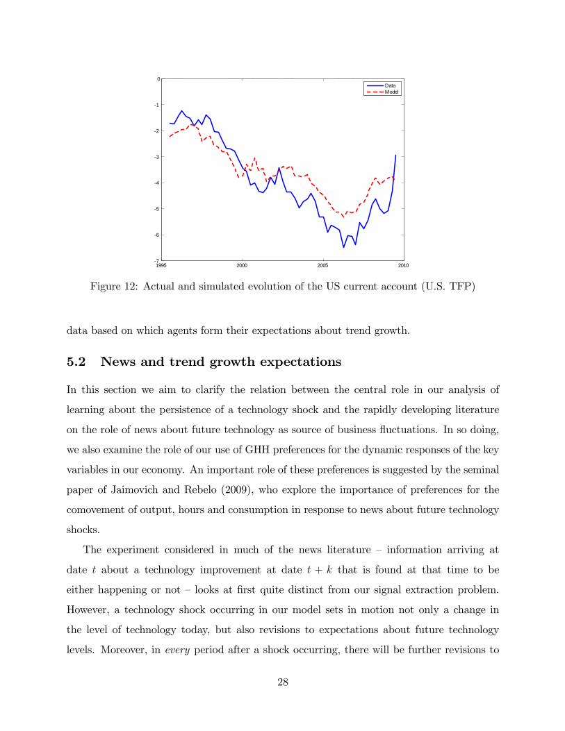
Figure 12 shows how the perceived future growth rate, based on the U.S. TFP process,

determines the model�s implied U.S. current account. Again, the solid blue line represents

the data, the dashed red line the model-implied evolution. It follows from the �gure that, for

the TFP estimates of Basu et al. as well, the simulated series matches the data quite closely.

Thus, we conclude that the evolution of the U.S. current account seems to be explained to

a large extent simply by changes in perceptions of trend growth, whether agents base their

estimates of trend growth on observations of labor productivity or of TFP.

We conclude from this that what matters are the perceived long-run trend growth rates to

explain the U.S. current account and output growth and not the speci�cs of the productivity

27

1995 2000 2005 2010­7

­6

­5

­4

­3

­2

­1

0DataModel

Figure 12: Actual and simulated evolution of the US current account (U.S. TFP)

data based on which agents form their expectations about trend growth.

5.2 News and trend growth expectations

In this section we aim to clarify the relation between the central role in our analysis of

learning about the persistence of a technology shock and the rapidly developing literature

on the role of news about future technology as source of business �uctuations. In so doing,

we also examine the role of our use of GHH preferences for the dynamic responses of the key

variables in our economy. An important role of these preferences is suggested by the seminal

paper of Jaimovich and Rebelo (2009), who explore the importance of preferences for the

comovement of output, hours and consumption in response to news about future technology

shocks.

The experiment considered in much of the news literature � information arriving at

date t about a technology improvement at date t + k that is found at that time to be

either happening or not �looks at �rst quite distinct from our signal extraction problem.

However, a technology shock occurring in our model sets in motion not only a change in

the level of technology today, but also revisions to expectations about future technology

levels. Moreover, in every period after a shock occurring, there will be further revisions to

28

expectations of technology in all future periods (although vanishing asymptotically). These

revisions are illustrated in Figures 13 and 14.

0 5 10 15 20 25 30 35 400

5

10

15

20

25

30

35Actual and expected technology level

Realized levelForecast at t=1Forecast at t=5Forecast at t=9Forecast at t=13Forecast at t=17

Figure 13: Revisions to expected log technology (Growth rate shock)

Figure 13 considers the case of a shock � to the growth rate of technology occurring at

date 1. At date 1, the log level of technology rises by 1. Because the signal-to-noise ratio

in our calibration is small, this shock is mostly seen as a permanent shift in the level to

technology, with very little consequences for future growth. As time goes by and agents

update their beliefs gtjt, not only are expectations of future levels of technology being revised

upwards, the slope of the expected trajectory of technology becomes more closely aligned

to the actual slope (the solid blue line) of the evolution of technology.Thus, in the spirit

of the news literature, in each period there are expectations of future, as yet unrealized,

technology increases that are being revised up from the previously held beliefs, and in each

period agents are surprised by the actual increase in the level of technology.

As shown in Figure 14, apart from the increase in the level of technology in the impact

period, the logic of revisions of beliefs works in reverse when the source of the technology

improvement is a one-o¤ increase ! in the level of technology.The initial small revision in the

estimate of gtjt caused by the shock leads to expectations of (albeit small) future technology

improvements that fail to materialize. The news process in our model is thus a case of

29

0 5 10 15 20 25 30 35 400

0.5

1

1.5

2

2.5

3

3.5Actual and expected technology level

Realized levelForecast at t=1Forecast at t=5Forecast at t=9Forecast at t=13Forecast at t=17

Figure 14: Revisions to expected log technology (Level shock)

what Walker and Leeper (2011) call �correlated news,�except that each shock in our model

triggers an in�nite sequence of such correlated news shocks, a new one in each period due to

the revision of gtjt. The impulse responses presented in Figure 6 can thus be viewed as the

sum of IRFs to a traditional technology shock and IRFs to a sequence of subsequent news

arrivals.

Given the close relation between technology shocks, be they level or growth rate shocks,

and perceived news about future technology, in Figure 15 we explore the role of information

and of our preference speci�cation for the response of hours to technology shocks.As high-

lighted by Jaimovich and Rebelo (2009), the class of preferences considered by King et al.

(1988) induces in response to expected future technology increases a decline in hours today

due to the wealth e¤ect on labor. This e¤ect is not present with the preferences considered

by Greenwood et al. (1988). In the class of preferences proposed by Jaimovich and Rebelo

that we use here, the parameter measures the strength of this wealth e¤ect, with = 1

corresponding to the King et al. preferences and = 0 to the preferences of Greenwood et

al. The responses shown in the left panels of Figure 15 are derived using = 1, those in the

left panels using a value of very close to 0.

Consider �rst the solid blue lines, which are the impulse responses derived under perfect

30

information about the nature of the shock. The upper two panels show that qualitatively

the hours responses to a one-o¤ permanent increase in the level of technology are quite

similar under the two preference speci�cations: Because consumption is permanently higher,

temporarily labor input falls, with this e¤ect being larger in the case of close to 0. The

lower two panels, by contrast, illustrate the e¤ect of the �news component�in a growth rate

shock on hours: With = 1 hours sharply decline due to the wealth e¤ect of expected future

productivity gains whereas with = 0 the opposite is the case.

0 20 40 60 80­4

­3

­2

­1

0

1x 10­3 Level shock, gamma=1

Quarters0 20 40 60 80

­5

0

5

10

15x 10­3

Quarters

Level shock, gamma=0.0075

imp. infoful l info

0 20 40 60 80­0.04

­0.03

­0.02

­0.01

0

0.01Growth rate shock, gamma=1

Quarters0 20 40 60 80

­0.1

­0.05

0

0.05

0.1

0.15

0.2

0.25Growth rate shock, gamma=0.0075

Quarters

Figure 15: IRFs of hours worked (Preferences and learning)

In the case of learning �the dashed red lines �the responses to a growth rate shock (the

lower two panels) are qualitatively similar to those under perfect information, due to the

constant arrival of positive news about future technology implied by the updating of beliefs

gtjt. The interesting case is that of a level shock. In the case of = 1 (the upper left panel)

the initial expectation of future technology increases (as shown by the forecast of technology

in the impact period, the �rst red dashed line in Figure 14) reinforces the negative impact

31

response under perfect information. By contrast, under GHH preferences (the upper right

panel) the expectation of future technology increases leads to an increase in hours that more

than o¤sets the negative e¤ect of the increase in technology upon impact. Over time, as the

expected technology increases fail to materialize, the response of hours turns negative.

6 Conclusions

In this paper we have argued that the evolution of the U.S. current account, and thus of

one side of what has been labelled �global imbalances,� can be largely explained within a

standard neoclassical growth model once changes in perceived trend growth rates in the

domestic and foreign economies are properly taken into account. Our sole departures from a

standard two-country real business cycle model are the assumption of a technology process

composed of two components of di¤erent persistence and the associated �ltering problem

that agents need to solve, and the use of preferences in the spirit of Jaimovich and Rebelo

(2009). As we have shown, the second assumption is relevant for improving our model�s �t of

output movements, whereas only the �rst assumption is necessary for explaining the current

account evolution.

It may seem odd, in the aftermath of the greatest �nancial crisis at least since the Great

Depression, to focus on an explanation that abstracts completely from �nancial factors.

First, we emphasize that we provide an explanation for the evolution of the current account,

not for the �nancial crisis. Second, we do not claim that �nancial innovation had no role

to play in facilitating the capital �ows from the rest of the world to the U.S. Rather, we

argue that it is important to �rst explore how far a simple, standard economic framework

together with careful modeling of agents�growth expectations can take us in understanding

these capital �ows.

Moreover, our conclusions seem particularly relevant in the current situation, in which

the economic policy debate is focused on regulatory reform so as to prevent a repeat of a

�nancial crisis of the dimension just seen. In the context of this debate, limits to current

account imbalances have been proposed as an essential element. Our analysis on the contrary

has shown that large current account de�cits can be the optimal response to relatively small

32

changes in trend growth rates. That said, for as long as agents need to take decisions under

imperfect knowledge of trend growth rates at home and abroad, it is inevitable that current

account movements will at times turn out to have been excessive, with all the concomitant

painful adjustment this entails.

Despite our emphasis on a frictionless framework, a natural next step would be to expand

our model by integrating a role for �nancial intermediation within and between countries

to better understand how changes in trend growth perceptions might interact with �nancial

structure. We leave this for future work.

References

[1] Aguiar, Mark, and Gita Gopinath, 2007. �Emerging Market Business Cycles: The Cycle

is the Trend.�Journal of Political Economy vol. 115(1), 69-102.

[2] Basu, Susanto, John Fernald, and Miles Kimball, 2006. �Are technology improvements

contractionary?�American Economic Review 96(5), 1418-1448.

[3] Baxter, Marianne, 1995. �International Trade and Business Cycles.�Ch. 35 in Gene

Grossman and Kenneth Rogo¤ (eds.), Handbook of International Economics Vol. 3, pp.

1801-1864. Amsterdam: Elsevier.

[4] Bernanke, Ben, 2005, �The Global Saving Glut and the U.S. Current Account De�cit.�

Speech, Federal Reserve Board

[5] Caballero, Ricardo, Emmanuel Farhi, and Pierre-Olivier Gourinchas, 2008. �An Equi-

librium Model of �Global Imbalances�and Low Interest Rates.�American Economic

Review 98(1), 358-93.

[6] Chen, Kaiji, Ayse ·Imrohoro¼glu, and Selahattin ·Imrohoro¼glu, 2009. �A quantitative as-

sessment of the decline in the U.S. current account.�Journal of Monetary Economics

56, 1135-47.

[7] Cooper, Richard, 2008. �Global Imbalances: Globalization, Demography, and Sustain-

ability.�Journal of Economic Perspectives 22(3), 93-112.

33

CFS Working Paper Series: No. Author(s) Title

2010/26 Ester Faia Credit Risk Transfers and the Macroeconomy

2010/25 Ignazio Angeloni Ester Faia Roland Winkler

Exit Strategies

2010/24 Roman Kräussl Andre Lucas Arjen Siegmann

Risk Aversion under Preference Uncertainty

2010/23 Carmen Lee Roman Kräussl Andre Lucas Leo Paas

Why Do Investors Sell Losers? How Adaptation to Losses Affects Future Capitulation Decisions

2010/22 Steffen Juranek Uwe Walz

Vertical Integration, Competition, and Financial Exchanges: Is there Grain in the Silo?

2010/21 Marcel Marekwica Michael Stamos

Optimal life cycle portfolio choice with housing market cycles

2010/20 Mahmoud Botshekan Roman Kraeussl Andre Lucas

Cash Flow and Discount Rate Risk in Up and Down Markets: What Is Actually Priced?

2010/19 Nikolaus Hautsch Peter Malec Melanie Schienle

Capturing the Zero: A New Class of Zero-Augmented Distributions and Multiplicative Error Processes

2010/18 Horst Entorf Christian Knoll Liliya Sattarova

Measuring Confidence and Uncertainty during the Financial Crisis: Evidence from the CFS Survey

Copies of working papers can be downloaded at http://www.ifk-cfs.de

[8] Edge, Rochelle, Thomas Laubach, and John Williams, 2007. �Learning and Shifts in

Long-Run Productivity Growth.�Journal of Monetary Economics 54 (8), 2421-2438.

[9] Engel, Charles, and John Rogers, 2006. �The U.S. current account de�cit and the

expected share of world output,�Journal of Monetary Economics 53

[10] Engel, Charles, and John Rogers, 2009. �Expected Consumption Growth from Cross-

Country Surveys: Implications for Assessing International Capital Markets.�IMF Sta¤

Papers 56, 543-573

[11] Erceg, Christopher, Luca Guerrieri, and Christopher Gust, 2006. �SIGMA: A New Open

Economy Model for Policy Analysis.�International Journal of Central Banking 2, 1-50.

[12] Feldstein, Martin, 2008. �Resolving the Global Imbalance: The Dollar and the U.S.

Saving Rate.�Journal of Economic Perspectives 22(3), 113-125.

[13] Ferrero, Andrea, 2010. �A structural decomposition of the U.S. trade balance: Produc-

tivity, demographics and �scal policy.�Journal of Monetary Economics 57, 478-490.

[14] Gilchrist and Saito, 2008. �Expectations, Asset Prices, and Monetary Policy: The Role

of Learning,� in J. Campbell (ed.), Asset Prices and Monetary Policy, University of

Chicago Press

[15] Glick, Reuben, and Kenneth Rogo¤, 1995. �Global versus country-speci�c productivity

shocks and the current account�, Journal of Monetary Economics 35, 159-92.

[16] Jaimovich, Nir, and Sergio Rebelo, 2009. �Can News about the Future Drive the Busi-

ness Cycle?�American Economic Review 99 (4), 1097-1118.

[17] Kahn, James, and Robert Rich, 2007. �Tracking the new economy: Using growth theory

to detect changes in trend productivity.�Journal of Monetary Economics 54, 1670-1701.

[18] Kollmann, Robert, 1996. �Incomplete Asset Markets and the Cross-Country Consump-

tion Correlation Puzzle�Journal of Economic Dynamics and Control 20, 945-62

34

[19] Laubach, Thomas, and John Williams, 2003. �Measuring the Natural Rate of Interest�.

The Review of Economics and Statistics 85(4) 1063-1070.

[20] Loretan, Mico, 2005. �Indexes of the foreign exchange value of the dollar�. Federal

Reserve Bulletin, Winter, 1-8

[21] Mendoza, Enrique, Vincenco Quadrini, and Victor Rios-Rull, 2009. �Financial Inte-

gration, Financial Development, and Global Imbalances�Journal of Political Economy

117(3)

[22] Nason, James, and John Rogers, 2006. �The present-value model of the current account

has been rejected: Round up the usual suspects�. Journal of International Economics

68, 159-187

[23] Obstfeld, Maurice, and Kenneth Rogo¤, 2007. �The Unsustainable U.S. Current Ac-

count De�cit Revisited.� in Richard H. Clarida, ed. G7 Current Account Imbalances:

Sustainability and Adjustment. Chicago University Press

[24] Obstfeld, Maurice, and Kenneth Rogo¤, 2010. �Global Imbalances and the Financial

Crisis: Products of Common Causes,�in: Reuven Glick andMark Spiegel, eds., Asia and

the Global Financial Crisis, conference volume, Federal Reserve Bank of San Francisco,

131-172

[25] Schmitt-Grohe, Stephanie, and Martin Uribe, 2008. �What�s News in Business Cycles?�

NBER working paper 14215

[26] Sims, Christopher, 2002. �Solving Linear Rational Expectation Models�. Computational

Economics 20, 1-20

[27] Smets, Frank, and Rafael Wouters, 2003. �An Estimated Dynamic Stochastic General

Equilibrium Model for the Euro Area�, Journal of the European Economic Association

1(5), 1123-1175

35

[28] Stock, James, and Mark Watson, 1998, �Business Cycle Fluctuations and U.S. Macro-

economic Time Series�, in John Taylor and Michael Woodford (eds.), Handbook of

Macroeconomics, vol. 1, chapter 1. Elsevier.

[29] Walker, Todd, and Eric Leeper, 2011, �Information �ows and news driven business

cycles�. Review of Economic Dynamics 14, 55-71.

36

CFS Working Paper Series: No. Author(s) Title

2010/26 Ester Faia Credit Risk Transfers and the Macroeconomy

2010/25 Ignazio Angeloni Ester Faia Roland Winkler

Exit Strategies

2010/24 Roman Kräussl Andre Lucas Arjen Siegmann

Risk Aversion under Preference Uncertainty

2010/23 Carmen Lee Roman Kräussl Andre Lucas Leo Paas

Why Do Investors Sell Losers? How Adaptation to Losses Affects Future Capitulation Decisions

2010/22 Steffen Juranek Uwe Walz

Vertical Integration, Competition, and Financial Exchanges: Is there Grain in the Silo?

2010/21 Marcel Marekwica Michael Stamos

Optimal life cycle portfolio choice with housing market cycles

2010/20 Mahmoud Botshekan Roman Kraeussl Andre Lucas

Cash Flow and Discount Rate Risk in Up and Down Markets: What Is Actually Priced?

2010/19 Nikolaus Hautsch Peter Malec Melanie Schienle

Capturing the Zero: A New Class of Zero-Augmented Distributions and Multiplicative Error Processes

2010/18 Horst Entorf Christian Knoll Liliya Sattarova

Measuring Confidence and Uncertainty during the Financial Crisis: Evidence from the CFS Survey

Copies of working papers can be downloaded at http://www.ifk-cfs.de