41
Maths in Motion Procedural animation in video games Danny Chapman Cumberland Lodge - February 2017 Version for distribution

Maths in MotionProcedural animation in video games
Danny ChapmanCumberland Lodge - February 2017
Version for distribution


Types of animation
Types of motion:
● Kinematic: Motion without regard to “physics” (mass or forces)● Dynamic: Motion as a result of forces
Methods:
● Forward: Generating motion given the starting point and controls● Inverse: Generating controls given the start and end states
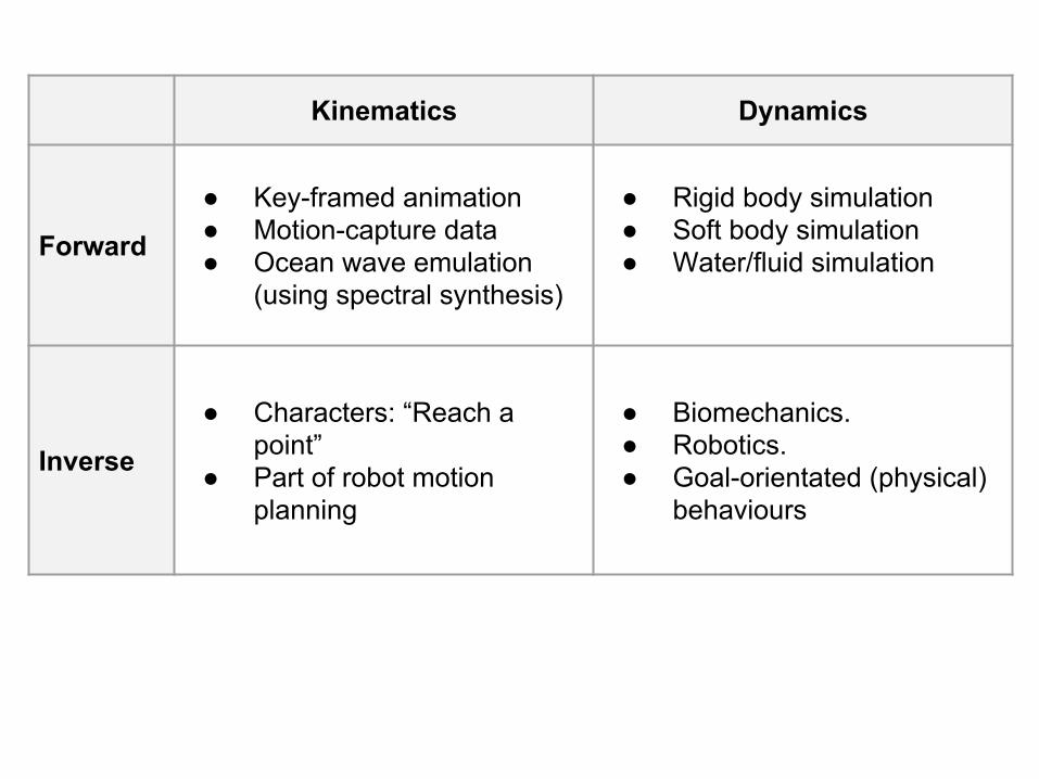
Kinematics Dynamics
Forward
● Key-framed animation● Motion-capture data● Ocean wave emulation
(using spectral synthesis)
● Rigid body simulation● Soft body simulation● Water/fluid simulation
Inverse
● Characters: “Reach a point”
● Part of robot motion planning
● Biomechanics.● Robotics.● Goal-orientated (physical)
behaviours

Clumsy Ninja
Forward kinematics
Inverse kinematics
Inverse dynamics
Forward dynamics


Navigating a skeletal hierarchy
Each bone coordinate frame indicates where it is relative to its parent, and how to transform points/frames into its parent space:
Point P can be expressed in frame 2F3 by 3P
If we want it in the world frame, then 0P = 0F1 1F2 2F3 3P
Where the Fs operate on their right (details depend on whether they are implemented as 4x4 matrices, quaternion plus translation etc.)
3PF1
F2 F3
0P
PF0
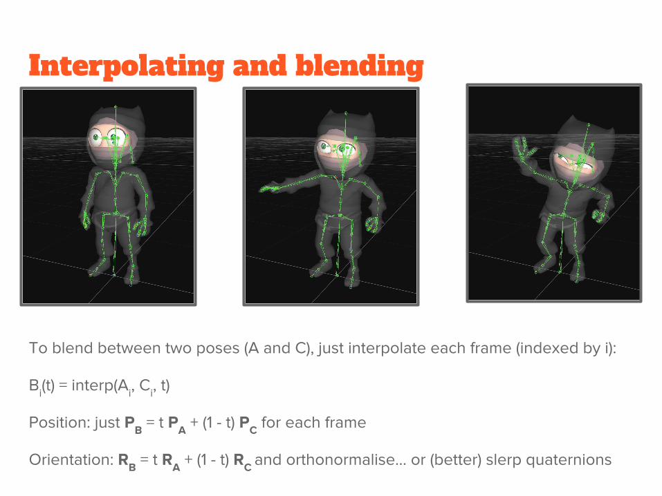
Interpolating and blending
To blend between two poses (A and C), just interpolate each frame (indexed by i):
Bi(t) = interp(Ai, Ci, t)
Position: just PB = t PA + (1 - t) PC for each frame
Orientation: RB = t RA + (1 - t) RC and orthonormalise... or (better) slerp quaternions

Motion matching
Three steps:
1. Record lots of motion (typically mocap)2. Each update, tell the system what kind of motion you want.3. System gives you a new animation frame that is consistent with:
a. What it was doing previouslyb. What you want.
Automatically select and play frames from a (long) animation clip containing all desired movement, based on a requested movement: No more blends and transitions!
Motion Field for Interactive Character Animation: Yongjoon Lee, Kevin Wampler, Gilbert Bernstein, Jovan Popović, Zoran Popović - ACM Transactions on Graphics 29(5) (SIGGRAPH Asia 2010)

Motion matching - preprocessing stepFor every frame in your source animation (40 minutes @ 30FPS = 72k frames):
● Calculate the velocity of the root● The trajectory out to 1 sec in the future● The trajectory back to 1 sec in the past● The position of a few bones relative to the root - e.g. the feet.
Big animation clip - 72k frames
Root motion from above:Extra data stored with each frame

Motion matching - at runtime
● Cost function measures the difference between each of the 72k candidate frames, and our current/history/predicted state.
● Pick the source frame that minimises the cost function.● 30 times a second per character (budget is < 1ms)!
Nice optimisation problem (e.g. nearest neighbours search to get candidates in an 18 dimensional space).
Predicted path
History
Current pose

Inverse Kinematics
If the chain starts at the origin, and each joint is determined by joint parameters θ1,...,θN (each 3x1) then the frame of the last joint (effector) is
0FN(θ1,...,θN) = 0F1(θ1) 1F2(θ2) ... N-1FN(θN)
Let the end joint be called an effector. Effector state vector is the position and world-space orientation of 0FN
s(θ1,...,θN) = [px py pz Ψ Θ Φ]T
If we have a target state t we want
s(θ1,...,θN) = t
Need to determine [θ1,...,θN] by inverting this relationship.

Approaches to IK
Methods
● Analytical/closed form - e.g. 2 links + pole vector● Blend based - interpolate N poses● Cyclic Coordinate Descent (CCD)● Jacobian inverse● Generic optimisation
Considerations
● Speed & memory● Style control - do animators like cost functions, or can they pass in a pose?● Handling of additional constraints (joint limits)● Behaviour with hard/impossible targets

Jacobian inverse solvers
Forwards kinematics equation:
s = f(Θ)
s is the position/orientation of an end effector (or multiple), Θ is the N joint angles in the chain(s).
Differentiate:
ds = df(Θ)/dΘ dΘ = J dΘ
6x1 = 6xN Nx1
Jacobian J tells us how s will move if the joint angles are changed.
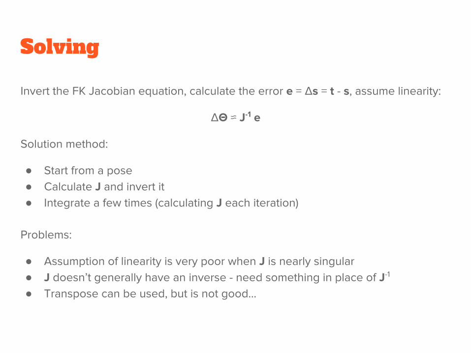
Solving
Invert the FK Jacobian equation, calculate the error e = ∆s = t - s, assume linearity:
∆Θ ≈ J-1 e
Solution method:
● Start from a pose● Calculate J and invert it● Integrate a few times (calculating J each iteration)
Problems:
● Assumption of linearity is very poor when J is nearly singular● J doesn’t generally have an inverse - need something in place of J-1
● Transpose can be used, but is not good...

Pseudo-inverse
J dΘ = ds
J dΘ = ( J JT) (J JT)-1 ds = J JT (J JT)-1 ds
dΘ = JT (J JT)-1 ds
dΘ = J✝ds with J✝ = JT (J JT)-1
● J is 6xN but J JT is 6x6● The pseudo-inverse is a true solution
Can improve behaviour near singularities using a damped least squares term:
J✝ = JT (J JT + λI)-1
Add additional terms to apply other constraints (centre of gravity), bias away from limits, null-space projection for redundancy control.

Ikinema - Recreate complete characters based on tracking a few body parts

Simulation of rigid bodies
Constant:
● Surface properties ● Mass and moments of inertia● Collision geometry (shape) - may or may not be the same as what is drawn.
Varying:
● Position P = [Px Py Pz]T
● Orientation R - 3x3 matrix or a quaternion● Velocity V = [Vx Vy Vz]
T
● Angular velocity w = (wx wy wz)T
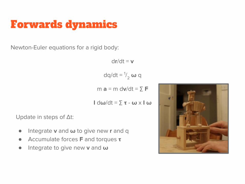
Forwards dynamics
Newton-Euler equations for a rigid body:
dr/dt = v
dq/dt = 1/2 ω q
m a = m dv/dt = ∑ F
I dω/dt = ∑ - ω x I ω
Update in steps of ∆t:
● Integrate v and ω to give new r and q● Accumulate forces F and torques ● Integrate to give new v and ω

Calculating forces and impulses
Impulse J = F ∆t
Inelastic collision so
want ∆v = -vv
Impulse J = m ∆v = -m v
Mass = m
Immovable object

Calculating impulsesTwo movable rigid bodies, single contact point:
● If frictionless then any impulse is normal to the contact● Apply impulse jc along N on body A (-jc on body B)● Desired change in relative velocity at contact: vc = N・∆vc
jc = me vc if vc > 0
jc = 0 otherwise
Where me is an effective mass - depends only on the geometry, mass and inertia properties.
N
A
B

Featherstone’s articulated body method
Featherstone’s method:
● Solves the unconstrained motion of the articulation as a single entity.● Response of the whole articulation to localised forces/impulses (like me).● Internal joint constraints cannot be violated.● Hard to understand and implement!
Maximal coordinates:
12 links 6 DoF for each
Simulate 72 DoF in total
Apply 11 revolute joint constraints to remove 33 DoF
Reduced coordinates:
Root link provides 6 DoF
11 revolute joints provide 33 DoF
Simulate 39 DoF.
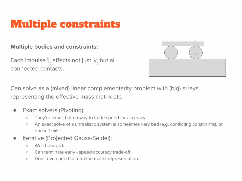
Multiple constraints
Multiple bodies and constraints:
Each impulse ijc affects not just ivc but all connected contacts.
Can solve as a (mixed) linear complementarity problem with (big) arrays representing the effective mass matrix etc.
● Exact solvers (Pivoting):○ They’re exact, but no way to trade speed for accuracy.○ An exact solve of a unrealistic system is sometimes very bad (e.g. conflicting constraints), or
doesn’t exist.
● Iterative (Projected Gauss-Seidel):○ Well behaved.○ Can terminate early - speed/accuracy trade-off.○ Don’t even need to form the matrix representation.

Control of physical characters
Realistic Modeling of Bird Flight Animations - Wu, J and Popović, Z

Complete list of games using optimal control techniques on characters:

Inverse Dynamics: Making things happen
Forwards Dynamics: Calculate motion given control inputs.
Inverse Dynamics: Calculate control inputs given observed/desired motion.
For games:
● Create a virtual stuntman
For biomechanics and robotics:
● Observed/desired motion may be known exactly.● Research in trajectory optimisation, underactuated robotics etc.

Dynamic control in games
Is this the future?
● Emergent gameplay● “Unique game moments”● Links with robotics, UAVs etc● We can cheat!
The challenges:
● Hard problem● Computationally expensive● Game designers lose control● Multiplayer and determinacy

Summary
Thanks to NaturalMotion - http://www.naturalmotion.com
and Clumsy Ninja (iOS and Android)

Internships and opportunities @ NaturalMotion: http://www.naturalmotion.com/
http://www.eurogamer.net/articles/2017-02-12-one-thing-about-gta4-has-never-been-bettered