532
MATLAB ® 7 Mathematics

MATLAB® 7Mathematics
How to Contact MathWorks
www.mathworks.com Webcomp.soft-sys.matlab Newsgroupwww.mathworks.com/contact_TS.html Technical Support
[email protected] Product enhancement [email protected] Bug [email protected] Documentation error [email protected] Order status, license renewals, [email protected] Sales, pricing, and general information
508-647-7000 (Phone)
508-647-7001 (Fax)
The MathWorks, Inc.3 Apple Hill DriveNatick, MA 01760-2098For contact information about worldwide offices, see the MathWorks Web site.
MATLAB® Mathematics
© COPYRIGHT 1984–2010 by The MathWorks, Inc.The software described in this document is furnished under a license agreement. The software may be usedor copied only under the terms of the license agreement. No part of this manual may be photocopied orreproduced in any form without prior written consent from The MathWorks, Inc.
FEDERAL ACQUISITION: This provision applies to all acquisitions of the Program and Documentationby, for, or through the federal government of the United States. By accepting delivery of the Programor Documentation, the government hereby agrees that this software or documentation qualifies ascommercial computer software or commercial computer software documentation as such terms are usedor defined in FAR 12.212, DFARS Part 227.72, and DFARS 252.227-7014. Accordingly, the terms andconditions of this Agreement and only those rights specified in this Agreement, shall pertain to and governthe use, modification, reproduction, release, performance, display, and disclosure of the Program andDocumentation by the federal government (or other entity acquiring for or through the federal government)and shall supersede any conflicting contractual terms or conditions. If this License fails to meet thegovernment’s needs or is inconsistent in any respect with federal procurement law, the government agreesto return the Program and Documentation, unused, to The MathWorks, Inc.
Trademarks
MATLAB and Simulink are registered trademarks of The MathWorks, Inc. Seewww.mathworks.com/trademarks for a list of additional trademarks. Other product or brandnames may be trademarks or registered trademarks of their respective holders.
Patents
MathWorks products are protected by one or more U.S. patents. Please seewww.mathworks.com/patents for more information.
Revision HistoryJune 2004 First printing New for MATLAB 7.0 (Release 14), formerly part of Using
MATLABOctober 2004 Online only Revised for MATLAB 7.0.1 (Release 14SP1)March 2005 Online only Revised for MATLAB 7.0.4 (Release 14SP2)June 2005 Second printing Minor revision for MATLAB 7.0.4September 2005 Second printing Revised for MATLAB 7.1 (Release 14SP3)March 2006 Second printing Revised for MATLAB 7.2 (Release 2006a)September 2006 Second printing Revised for MATLAB 7.3 (Release 2006b)September 2007 Online only Revised for MATLAB 7.5 (Release 2007b)March 2008 Online only Revised for MATLAB 7.6 (Release 2008a)October 2008 Online only Revised for MATLAB 7.7 (Release 2008b)March 2009 Online only Revised for MATLAB 7.8 (Release 2009a)September 2009 Online only Revised for MATLAB 7.9 (Release 2009b)March 2010 Online only Revised for MATLAB 7.10 (Release 2010a)September 2010 Online only Revised for MATLAB 7.11 (Release 2010b)

Contents
Matrices and Arrays
1Creating and Concatenating Matrices . . . . . . . . . . . . . . . 1-2Overview . . . . . . . . . . . . . . . . . . . . . . . . . . . . . . . . . . . . . . . . 1-2Constructing a Simple Matrix . . . . . . . . . . . . . . . . . . . . . . . 1-3Specialized Matrix Functions . . . . . . . . . . . . . . . . . . . . . . . . 1-4Concatenating Matrices . . . . . . . . . . . . . . . . . . . . . . . . . . . . 1-6Matrix Concatenation Functions . . . . . . . . . . . . . . . . . . . . . 1-7Generating a Numeric Sequence . . . . . . . . . . . . . . . . . . . . . 1-9
Matrix Indexing . . . . . . . . . . . . . . . . . . . . . . . . . . . . . . . . . . . 1-12Accessing Single Elements . . . . . . . . . . . . . . . . . . . . . . . . . . 1-12Linear Indexing . . . . . . . . . . . . . . . . . . . . . . . . . . . . . . . . . . . 1-13Functions That Control Indexing Style . . . . . . . . . . . . . . . . 1-13Accessing Multiple Elements . . . . . . . . . . . . . . . . . . . . . . . . 1-14Using Logicals in Array Indexing . . . . . . . . . . . . . . . . . . . . 1-17Single-Colon Indexing with Different Array Types . . . . . . . 1-20Indexing on Assignment . . . . . . . . . . . . . . . . . . . . . . . . . . . . 1-21
Getting Information About a Matrix . . . . . . . . . . . . . . . . . 1-22Dimensions of the Matrix . . . . . . . . . . . . . . . . . . . . . . . . . . . 1-22Classes Used in the Matrix . . . . . . . . . . . . . . . . . . . . . . . . . . 1-23Data Structures Used in the Matrix . . . . . . . . . . . . . . . . . . 1-24
Resizing and Reshaping Matrices . . . . . . . . . . . . . . . . . . . 1-25Expanding the Size of a Matrix . . . . . . . . . . . . . . . . . . . . . . 1-25Diminishing the Size of a Matrix . . . . . . . . . . . . . . . . . . . . . 1-29Reshaping a Matrix . . . . . . . . . . . . . . . . . . . . . . . . . . . . . . . . 1-30Preallocating Memory . . . . . . . . . . . . . . . . . . . . . . . . . . . . . . 1-32
Shifting and Sorting Matrices . . . . . . . . . . . . . . . . . . . . . . 1-35Shift and Sort Functions . . . . . . . . . . . . . . . . . . . . . . . . . . . . 1-35Shifting the Location of Matrix Elements . . . . . . . . . . . . . . 1-35Sorting the Data in Each Column . . . . . . . . . . . . . . . . . . . . 1-37Sorting the Data in Each Row . . . . . . . . . . . . . . . . . . . . . . . 1-37Sorting Row Vectors . . . . . . . . . . . . . . . . . . . . . . . . . . . . . . . 1-38
v
Operating on Diagonal Matrices . . . . . . . . . . . . . . . . . . . . 1-40Diagonal Matrix Functions . . . . . . . . . . . . . . . . . . . . . . . . . . 1-40Constructing a Matrix from a Diagonal Vector . . . . . . . . . . 1-40Returning a Triangular Portion of a Matrix . . . . . . . . . . . . 1-41Concatenating Matrices Diagonally . . . . . . . . . . . . . . . . . . . 1-41
Empty Matrices, Scalars, and Vectors . . . . . . . . . . . . . . . 1-42Overview . . . . . . . . . . . . . . . . . . . . . . . . . . . . . . . . . . . . . . . . 1-42The Empty Matrix . . . . . . . . . . . . . . . . . . . . . . . . . . . . . . . . . 1-43Scalars . . . . . . . . . . . . . . . . . . . . . . . . . . . . . . . . . . . . . . . . . . 1-45Vectors . . . . . . . . . . . . . . . . . . . . . . . . . . . . . . . . . . . . . . . . . . 1-46
Full and Sparse Matrices . . . . . . . . . . . . . . . . . . . . . . . . . . . 1-48Overview . . . . . . . . . . . . . . . . . . . . . . . . . . . . . . . . . . . . . . . . 1-48Sparse Matrix Functions . . . . . . . . . . . . . . . . . . . . . . . . . . . 1-48
Multidimensional Arrays . . . . . . . . . . . . . . . . . . . . . . . . . . . 1-50Overview . . . . . . . . . . . . . . . . . . . . . . . . . . . . . . . . . . . . . . . . 1-50Creating Multidimensional Arrays . . . . . . . . . . . . . . . . . . . 1-52Accessing Multidimensional Array Properties . . . . . . . . . . 1-56Indexing Multidimensional Arrays . . . . . . . . . . . . . . . . . . . 1-56Reshaping Multidimensional Arrays . . . . . . . . . . . . . . . . . . 1-60Permuting Array Dimensions . . . . . . . . . . . . . . . . . . . . . . . . 1-62Computing with Multidimensional Arrays . . . . . . . . . . . . . 1-64Organizing Data in Multidimensional Arrays . . . . . . . . . . . 1-65Multidimensional Cell Arrays . . . . . . . . . . . . . . . . . . . . . . . 1-67Multidimensional Structure Arrays . . . . . . . . . . . . . . . . . . . 1-68
Summary of Matrix and Array Functions . . . . . . . . . . . . 1-70
Linear Algebra
2MATLAB Linear Algebra Functions . . . . . . . . . . . . . . . . . 2-2
Matrices in the MATLAB Environment . . . . . . . . . . . . . . 2-5Creating Matrices . . . . . . . . . . . . . . . . . . . . . . . . . . . . . . . . . 2-5Adding and Subtracting Matrices . . . . . . . . . . . . . . . . . . . . 2-7
vi Contents
Vector Products and Transpose . . . . . . . . . . . . . . . . . . . . . . 2-7Multiplying Matrices . . . . . . . . . . . . . . . . . . . . . . . . . . . . . . 2-9Identity Matrix . . . . . . . . . . . . . . . . . . . . . . . . . . . . . . . . . . . 2-11Kronecker Tensor Product . . . . . . . . . . . . . . . . . . . . . . . . . . 2-12Vector and Matrix Norms . . . . . . . . . . . . . . . . . . . . . . . . . . . 2-13Using Multithreaded Computation with Linear AlgebraFunctions . . . . . . . . . . . . . . . . . . . . . . . . . . . . . . . . . . . . . . 2-14
Systems of Linear Equations . . . . . . . . . . . . . . . . . . . . . . . . 2-15Computational Considerations . . . . . . . . . . . . . . . . . . . . . . . 2-15The mldivide Algorithm . . . . . . . . . . . . . . . . . . . . . . . . . . . . 2-17General Solution . . . . . . . . . . . . . . . . . . . . . . . . . . . . . . . . . . 2-18Square Systems . . . . . . . . . . . . . . . . . . . . . . . . . . . . . . . . . . . 2-18Overdetermined Systems . . . . . . . . . . . . . . . . . . . . . . . . . . . 2-21Using Multithreaded Computation with Systems of LinearEquations . . . . . . . . . . . . . . . . . . . . . . . . . . . . . . . . . . . . . 2-24
Iterative Methods for Solving Systems of LinearEquations . . . . . . . . . . . . . . . . . . . . . . . . . . . . . . . . . . . . . 2-25
Inverses and Determinants . . . . . . . . . . . . . . . . . . . . . . . . . 2-26Introduction . . . . . . . . . . . . . . . . . . . . . . . . . . . . . . . . . . . . . . 2-26Pseudoinverses . . . . . . . . . . . . . . . . . . . . . . . . . . . . . . . . . . . 2-27
Factorizations . . . . . . . . . . . . . . . . . . . . . . . . . . . . . . . . . . . . . 2-31Introduction . . . . . . . . . . . . . . . . . . . . . . . . . . . . . . . . . . . . . . 2-31Cholesky Factorization . . . . . . . . . . . . . . . . . . . . . . . . . . . . . 2-31LU Factorization . . . . . . . . . . . . . . . . . . . . . . . . . . . . . . . . . . 2-33QR Factorization . . . . . . . . . . . . . . . . . . . . . . . . . . . . . . . . . . 2-34Using Multithreaded Computation for Factorization . . . . . 2-38
Powers and Exponentials . . . . . . . . . . . . . . . . . . . . . . . . . . 2-40Positive Integer Powers . . . . . . . . . . . . . . . . . . . . . . . . . . . . 2-40Inverse and Fractional Powers . . . . . . . . . . . . . . . . . . . . . . . 2-40Element-by-Element Powers . . . . . . . . . . . . . . . . . . . . . . . . 2-41Exponentials . . . . . . . . . . . . . . . . . . . . . . . . . . . . . . . . . . . . . 2-41
Eigenvalues . . . . . . . . . . . . . . . . . . . . . . . . . . . . . . . . . . . . . . . 2-44Eigenvalue Decomposition . . . . . . . . . . . . . . . . . . . . . . . . . . 2-44Multiple Eigenvalues . . . . . . . . . . . . . . . . . . . . . . . . . . . . . . 2-45Schur Decomposition . . . . . . . . . . . . . . . . . . . . . . . . . . . . . . 2-46
vii
Singular Values . . . . . . . . . . . . . . . . . . . . . . . . . . . . . . . . . . . 2-48
Random Numbers
3Generating Random Numbers . . . . . . . . . . . . . . . . . . . . . . 3-2
Managing the Default Stream . . . . . . . . . . . . . . . . . . . . . . . 3-3Random Number Data Types . . . . . . . . . . . . . . . . . . . . . . . . 3-8
Creating and Controlling a Random Number Stream . . 3-10Substreams . . . . . . . . . . . . . . . . . . . . . . . . . . . . . . . . . . . . . . 3-11Choosing a Random Number Generator . . . . . . . . . . . . . . . 3-12Compatibility Considerations . . . . . . . . . . . . . . . . . . . . . . . . 3-16
Multiple streams . . . . . . . . . . . . . . . . . . . . . . . . . . . . . . . . . . 3-19
Updating Your Random Number Generator Syntax . . . 3-22Legacy Random Stream . . . . . . . . . . . . . . . . . . . . . . . . . . . . 3-24
Selected Bibliography . . . . . . . . . . . . . . . . . . . . . . . . . . . . . . 3-26
Sparse Matrices
4Function Summary . . . . . . . . . . . . . . . . . . . . . . . . . . . . . . . . 4-2Functions That Support Sparse Matrices . . . . . . . . . . . . . . 4-2Functions That Do Not Support Sparse Matrices . . . . . . . . 4-6Functions with Sparse Alternatives . . . . . . . . . . . . . . . . . . . 4-10
Computational Advantages . . . . . . . . . . . . . . . . . . . . . . . . . 4-10Memory Management . . . . . . . . . . . . . . . . . . . . . . . . . . . . . . 4-10Computational Efficiency . . . . . . . . . . . . . . . . . . . . . . . . . . . 4-11
viii Contents
Constructing Sparse Matrices . . . . . . . . . . . . . . . . . . . . . . 4-13Creating Sparse Matrices . . . . . . . . . . . . . . . . . . . . . . . . . . . 4-13Importing Sparse Matrices . . . . . . . . . . . . . . . . . . . . . . . . . . 4-18
Accessing Sparse Matrices . . . . . . . . . . . . . . . . . . . . . . . . . . 4-19Nonzero Elements . . . . . . . . . . . . . . . . . . . . . . . . . . . . . . . . . 4-19Indices and Values . . . . . . . . . . . . . . . . . . . . . . . . . . . . . . . . 4-21Indexing in Sparse Matrix Operations . . . . . . . . . . . . . . . . 4-21Visualizing Sparse Matrices . . . . . . . . . . . . . . . . . . . . . . . . . 4-24
Sparse Matrix Operations . . . . . . . . . . . . . . . . . . . . . . . . . . 4-25Efficiency of Operations . . . . . . . . . . . . . . . . . . . . . . . . . . . . 4-25Permutations and Reordering . . . . . . . . . . . . . . . . . . . . . . . 4-26Factoring Sparse Matrices . . . . . . . . . . . . . . . . . . . . . . . . . . 4-30Systems of Linear Equations . . . . . . . . . . . . . . . . . . . . . . . . 4-37Eigenvalues and Singular Values . . . . . . . . . . . . . . . . . . . . 4-40Performance Limitations . . . . . . . . . . . . . . . . . . . . . . . . . . . 4-42
Selected Bibliography . . . . . . . . . . . . . . . . . . . . . . . . . . . . . . 4-45
Functions of One Variable
5Function Summary . . . . . . . . . . . . . . . . . . . . . . . . . . . . . . . . 5-2
Representing Polynomials . . . . . . . . . . . . . . . . . . . . . . . . . . 5-3
Evaluating Polynomials . . . . . . . . . . . . . . . . . . . . . . . . . . . . 5-4
Roots of Polynomials . . . . . . . . . . . . . . . . . . . . . . . . . . . . . . . 5-5
Roots of Scalar Functions . . . . . . . . . . . . . . . . . . . . . . . . . . 5-6Solving a Nonlinear Equation in One Variable . . . . . . . . . . 5-6Using a Starting Interval . . . . . . . . . . . . . . . . . . . . . . . . . . . 5-8Using a Starting Point . . . . . . . . . . . . . . . . . . . . . . . . . . . . . 5-9
Derivatives . . . . . . . . . . . . . . . . . . . . . . . . . . . . . . . . . . . . . . . 5-12
ix
Convolution . . . . . . . . . . . . . . . . . . . . . . . . . . . . . . . . . . . . . . . 5-13
Partial Fraction Expansions . . . . . . . . . . . . . . . . . . . . . . . . 5-14
Polynomial Curve Fitting . . . . . . . . . . . . . . . . . . . . . . . . . . 5-15
Characteristic Polynomials . . . . . . . . . . . . . . . . . . . . . . . . . 5-17
Computational Geometry
6Overview . . . . . . . . . . . . . . . . . . . . . . . . . . . . . . . . . . . . . . . . . 6-2
Triangulation Representations . . . . . . . . . . . . . . . . . . . . . 6-32-D and 3-D Domains . . . . . . . . . . . . . . . . . . . . . . . . . . . . . . 6-3Triangulation Face-Vertex Format . . . . . . . . . . . . . . . . . . . 6-5Querying Triangulations Using TriRep . . . . . . . . . . . . . . . . 6-7
Delaunay Triangulation . . . . . . . . . . . . . . . . . . . . . . . . . . . . 6-17Definition of Delaunay Triangulation . . . . . . . . . . . . . . . . . 6-17Creating Delaunay Triangulations . . . . . . . . . . . . . . . . . . . 6-19Triangulation of Point Sets Containing DuplicateLocations . . . . . . . . . . . . . . . . . . . . . . . . . . . . . . . . . . . . . . 6-44
Spatial Searching . . . . . . . . . . . . . . . . . . . . . . . . . . . . . . . . . . 6-47Introduction . . . . . . . . . . . . . . . . . . . . . . . . . . . . . . . . . . . . . . 6-47Nearest-Neighbor Search . . . . . . . . . . . . . . . . . . . . . . . . . . . 6-47Point Location . . . . . . . . . . . . . . . . . . . . . . . . . . . . . . . . . . . . 6-50Searching Non-Delaunay Triangulations . . . . . . . . . . . . . . 6-53
Voronoi Diagrams . . . . . . . . . . . . . . . . . . . . . . . . . . . . . . . . . 6-57Computing the Voronoi Diagram . . . . . . . . . . . . . . . . . . . . . 6-61
Convex Hulls . . . . . . . . . . . . . . . . . . . . . . . . . . . . . . . . . . . . . . 6-66Computing the Convex Hull . . . . . . . . . . . . . . . . . . . . . . . . . 6-67
x Contents
Interpolation
7Interpolating Structured Data . . . . . . . . . . . . . . . . . . . . . . 7-3One-Dimensional Data . . . . . . . . . . . . . . . . . . . . . . . . . . . . . 7-3Two-Dimensional Data . . . . . . . . . . . . . . . . . . . . . . . . . . . . . 7-5Multidimensional Data . . . . . . . . . . . . . . . . . . . . . . . . . . . . . 7-8
Interpolating Scattered Data . . . . . . . . . . . . . . . . . . . . . . . 7-12Scattered Data . . . . . . . . . . . . . . . . . . . . . . . . . . . . . . . . . . . . 7-12Interpolating Scattered Data Using griddata andgriddatan . . . . . . . . . . . . . . . . . . . . . . . . . . . . . . . . . . . . . . 7-15
Interpolating Scattered Data Using the TriScatteredInterpClass . . . . . . . . . . . . . . . . . . . . . . . . . . . . . . . . . . . . . . . . . 7-19
Addressing Problems in Scattered Data Interpolation . . . . 7-32
Optimization
8Function Summary . . . . . . . . . . . . . . . . . . . . . . . . . . . . . . . . 8-2
Optimizing Nonlinear Functions . . . . . . . . . . . . . . . . . . . . 8-3Minimizing Functions of One Variable . . . . . . . . . . . . . . . . 8-3Minimizing Functions of Several Variables . . . . . . . . . . . . . 8-5fminsearch Algorithm . . . . . . . . . . . . . . . . . . . . . . . . . . . . . . 8-5Maximizing Functions . . . . . . . . . . . . . . . . . . . . . . . . . . . . . 8-7
Example: Curve Fitting via Optimization . . . . . . . . . . . . 8-9Curve Fitting by Optimization . . . . . . . . . . . . . . . . . . . . . . . 8-9Creating an Example File . . . . . . . . . . . . . . . . . . . . . . . . . . . 8-9Running the Example . . . . . . . . . . . . . . . . . . . . . . . . . . . . . . 8-10Plotting the Results . . . . . . . . . . . . . . . . . . . . . . . . . . . . . . . 8-10
Setting Options . . . . . . . . . . . . . . . . . . . . . . . . . . . . . . . . . . . . 8-12
Iterative Display . . . . . . . . . . . . . . . . . . . . . . . . . . . . . . . . . . 8-14
xi
Output Functions . . . . . . . . . . . . . . . . . . . . . . . . . . . . . . . . . . 8-16What Is an Output Function? . . . . . . . . . . . . . . . . . . . . . . . . 8-16Creating and Using an Output Function . . . . . . . . . . . . . . . 8-16Structure of the Output Function . . . . . . . . . . . . . . . . . . . . 8-18Example of a Nested Output Function . . . . . . . . . . . . . . . . 8-19Fields in optimValues . . . . . . . . . . . . . . . . . . . . . . . . . . . . . . 8-21States of the Algorithm . . . . . . . . . . . . . . . . . . . . . . . . . . . . . 8-21Stop Flag . . . . . . . . . . . . . . . . . . . . . . . . . . . . . . . . . . . . . . . . 8-22
Plot Functions . . . . . . . . . . . . . . . . . . . . . . . . . . . . . . . . . . . . 8-24What Is A Plot Function? . . . . . . . . . . . . . . . . . . . . . . . . . . . 8-24Example: Plot Function . . . . . . . . . . . . . . . . . . . . . . . . . . . . 8-25
Troubleshooting and Tips . . . . . . . . . . . . . . . . . . . . . . . . . . 8-27
Reference . . . . . . . . . . . . . . . . . . . . . . . . . . . . . . . . . . . . . . . . . 8-29
Function Handles
9Introduction . . . . . . . . . . . . . . . . . . . . . . . . . . . . . . . . . . . . . . 9-2
Defining Functions In Files . . . . . . . . . . . . . . . . . . . . . . . . . 9-3
Anonymous Functions . . . . . . . . . . . . . . . . . . . . . . . . . . . . . 9-4
Example: Function Plotting Function . . . . . . . . . . . . . . . 9-5
Parameterizing Functions . . . . . . . . . . . . . . . . . . . . . . . . . . 9-8Using Nested Functions . . . . . . . . . . . . . . . . . . . . . . . . . . . . 9-8Using Anonymous Functions . . . . . . . . . . . . . . . . . . . . . . . . 9-9
xii Contents
Calculus
10Ordinary Differential Equations . . . . . . . . . . . . . . . . . . . . 10-2Function Summary . . . . . . . . . . . . . . . . . . . . . . . . . . . . . . . . 10-2Initial Value Problems . . . . . . . . . . . . . . . . . . . . . . . . . . . . . 10-4Types of Solvers . . . . . . . . . . . . . . . . . . . . . . . . . . . . . . . . . . . 10-6Solver Syntax . . . . . . . . . . . . . . . . . . . . . . . . . . . . . . . . . . . . 10-8Integrator Options . . . . . . . . . . . . . . . . . . . . . . . . . . . . . . . . 10-9Examples . . . . . . . . . . . . . . . . . . . . . . . . . . . . . . . . . . . . . . . . 10-10Troubleshooting . . . . . . . . . . . . . . . . . . . . . . . . . . . . . . . . . . . 10-39
Delay Differential Equations . . . . . . . . . . . . . . . . . . . . . . . 10-47Function Summary . . . . . . . . . . . . . . . . . . . . . . . . . . . . . . . . 10-47Initial Value Problems . . . . . . . . . . . . . . . . . . . . . . . . . . . . . 10-48Types of Solvers . . . . . . . . . . . . . . . . . . . . . . . . . . . . . . . . . . . 10-49Discontinuities . . . . . . . . . . . . . . . . . . . . . . . . . . . . . . . . . . . 10-50Integrator Options . . . . . . . . . . . . . . . . . . . . . . . . . . . . . . . . 10-51Examples . . . . . . . . . . . . . . . . . . . . . . . . . . . . . . . . . . . . . . . . 10-51
Boundary-Value Problems . . . . . . . . . . . . . . . . . . . . . . . . . . 10-59Function Summary . . . . . . . . . . . . . . . . . . . . . . . . . . . . . . . . 10-59Boundary Value Problems . . . . . . . . . . . . . . . . . . . . . . . . . . 10-60BVP Solver . . . . . . . . . . . . . . . . . . . . . . . . . . . . . . . . . . . . . . . 10-61Integrator Options . . . . . . . . . . . . . . . . . . . . . . . . . . . . . . . . 10-64Examples . . . . . . . . . . . . . . . . . . . . . . . . . . . . . . . . . . . . . . . . 10-65
Partial Differential Equations . . . . . . . . . . . . . . . . . . . . . . 10-87Function Summary . . . . . . . . . . . . . . . . . . . . . . . . . . . . . . . . 10-87Initial Value Problems . . . . . . . . . . . . . . . . . . . . . . . . . . . . . 10-88PDE Solver . . . . . . . . . . . . . . . . . . . . . . . . . . . . . . . . . . . . . . 10-89Integrator Options . . . . . . . . . . . . . . . . . . . . . . . . . . . . . . . . 10-92Examples . . . . . . . . . . . . . . . . . . . . . . . . . . . . . . . . . . . . . . . . 10-93
Selected Bibliography for Differential Equations . . . . . 10-105
Integration . . . . . . . . . . . . . . . . . . . . . . . . . . . . . . . . . . . . . . . . 10-106Quadrature Functions . . . . . . . . . . . . . . . . . . . . . . . . . . . . . 10-106Example: Arc Length . . . . . . . . . . . . . . . . . . . . . . . . . . . . . . 10-107Example: Double Integration . . . . . . . . . . . . . . . . . . . . . . . . 10-107
xiii
Fourier Transforms
11Discrete Fourier Transform (DFT) . . . . . . . . . . . . . . . . . . 11-2Introduction . . . . . . . . . . . . . . . . . . . . . . . . . . . . . . . . . . . . . . 11-2Visualizing the DFT . . . . . . . . . . . . . . . . . . . . . . . . . . . . . . . 11-3
Fast Fourier Transform (FFT) . . . . . . . . . . . . . . . . . . . . . . 11-8Introduction . . . . . . . . . . . . . . . . . . . . . . . . . . . . . . . . . . . . . . 11-8The FFT in One Dimension . . . . . . . . . . . . . . . . . . . . . . . . . 11-9The FFT in Multiple Dimensions . . . . . . . . . . . . . . . . . . . . . 11-23
Function Summary . . . . . . . . . . . . . . . . . . . . . . . . . . . . . . . . 11-28
Index
xiv Contents
1
Matrices and Arrays
• “Creating and Concatenating Matrices” on page 1-2
• “Matrix Indexing” on page 1-12
• “Getting Information About a Matrix” on page 1-22
• “Resizing and Reshaping Matrices” on page 1-25
• “Shifting and Sorting Matrices” on page 1-35
• “Operating on Diagonal Matrices” on page 1-40
• “Empty Matrices, Scalars, and Vectors” on page 1-42
• “Full and Sparse Matrices” on page 1-48
• “Multidimensional Arrays” on page 1-50
• “Summary of Matrix and Array Functions” on page 1-70

1 Matrices and Arrays
Creating and Concatenating Matrices
In this section...
“Overview” on page 1-2
“Constructing a Simple Matrix” on page 1-3
“Specialized Matrix Functions” on page 1-4
“Concatenating Matrices” on page 1-6
“Matrix Concatenation Functions” on page 1-7
“Generating a Numeric Sequence” on page 1-9
OverviewThe most basic MATLAB® data structure is the matrix: a two-dimensional,rectangularly shaped data structure capable of storing multiple elements ofdata in an easily accessible format. These data elements can be numbers,characters, logical states of true or false, or even other MATLAB structuretypes. MATLAB uses these two-dimensional matrices to store single numbersand linear series of numbers as well. In these cases, the dimensions are 1-by-1and 1-by-n respectively, where n is the length of the numeric series. MATLABalso supports data structures that have more than two dimensions. Thesedata structures are referred to as arrays in the MATLAB documentation.
MATLAB is a matrix-based computing environment. All of the data that youenter into MATLAB is stored in the form of a matrix or a multidimensionalarray. Even a single numeric value like 100 is stored as a matrix (in this case,a matrix having dimensions 1-by-1):
A = 100;
whos AName Size Bytes Class
A 1x1 8 double array
Regardless of the class being used, whether it is numeric, character, or logicaltrue or false data, MATLAB stores this data in matrix (or array) form. Forexample, the string 'Hello World' is a 1-by-11 matrix of individual character
1-2
Creating and Concatenating Matrices
elements in MATLAB. You can also build matrices composed of more complexclasses, such as MATLAB structures and cell arrays.
To create a matrix of basic data elements such as numbers or characters, see
• “Constructing a Simple Matrix” on page 1-3
• “Specialized Matrix Functions” on page 1-4
To build a matrix composed of other matrices, see
• “Concatenating Matrices” on page 1-6
• “Matrix Concatenation Functions” on page 1-7
This section also describes
• “Generating a Numeric Sequence” on page 1-9
• “Combining Unlike Classes”
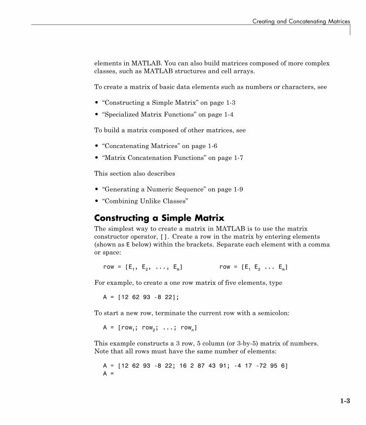
Constructing a Simple MatrixThe simplest way to create a matrix in MATLAB is to use the matrixconstructor operator, []. Create a row in the matrix by entering elements(shown as E below) within the brackets. Separate each element with a commaor space:
row = [E1, E2, ..., Em] row = [E1 E2 ... Em]
For example, to create a one row matrix of five elements, type
A = [12 62 93 -8 22];
To start a new row, terminate the current row with a semicolon:
A = [row1; row2; ...; rown]
This example constructs a 3 row, 5 column (or 3-by-5) matrix of numbers.Note that all rows must have the same number of elements:
A = [12 62 93 -8 22; 16 2 87 43 91; -4 17 -72 95 6]A =
1-3
1 Matrices and Arrays
12 62 93 -8 2216 2 87 43 91-4 17 -72 95 6
The square brackets operator constructs two-dimensional matrices only,(including 0-by-0, 1-by-1, and 1-by-n matrices). To construct arrays of morethan two dimensions, see “Creating Multidimensional Arrays” on page 1-52.
For instructions on how to read or overwrite any matrix element, see “MatrixIndexing” on page 1-12.
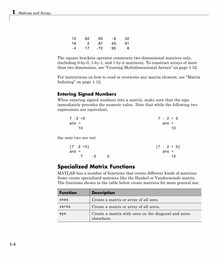
Entering Signed NumbersWhen entering signed numbers into a matrix, make sure that the signimmediately precedes the numeric value. Note that while the following twoexpressions are equivalent,
7 -2 +5 7 - 2 + 5ans = ans =
10 10
the next two are not:
[7 -2 +5] [7 - 2 + 5]ans = ans =
7 -2 5 10
Specialized Matrix FunctionsMATLAB has a number of functions that create different kinds of matrices.Some create specialized matrices like the Hankel or Vandermonde matrix.The functions shown in the table below create matrices for more general use.
Function Description
ones Create a matrix or array of all ones.
zeros Create a matrix or array of all zeros.
eye Create a matrix with ones on the diagonal and zeroselsewhere.
1-4
Creating and Concatenating Matrices
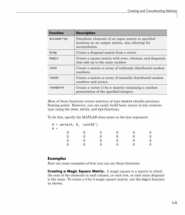
Function Description
accumarray Distribute elements of an input matrix to specifiedlocations in an output matrix, also allowing foraccumulation.
diag Create a diagonal matrix from a vector.
magic Create a square matrix with rows, columns, and diagonalsthat add up to the same number.
rand Create a matrix or array of uniformly distributed randomnumbers.
randn Create a matrix or array of normally distributed randomnumbers and arrays.
randperm Create a vector (1-by-n matrix) containing a randompermutation of the specified integers.
Most of these functions return matrices of type double (double-precisionfloating point). However, you can easily build basic arrays of any numerictype using the ones, zeros, and eye functions.
To do this, specify the MATLAB class name as the last argument:
A = zeros(4, 6, 'uint32')A =
0 0 0 0 0 00 0 0 0 0 00 0 0 0 0 00 0 0 0 0 0
ExamplesHere are some examples of how you can use these functions.
Creating a Magic Square Matrix. A magic square is a matrix in whichthe sum of the elements in each column, or each row, or each main diagonalis the same. To create a 5-by-5 magic square matrix, use the magic functionas shown.
1-5

1 Matrices and Arrays
A = magic(5)A =
17 24 1 8 1523 5 7 14 164 6 13 20 22
10 12 19 21 311 18 25 2 9
Note that the elements of each row, each column, and each main diagonaladd up to the same value: 65.
Creating a Diagonal Matrix. Use diag to create a diagonal matrix from avector. You can place the vector along the main diagonal of the matrix, or on adiagonal that is above or below the main one, as shown here. The -1 inputplaces the vector one row below the main diagonal:
A = [12 62 93 -8 22];
B = diag(A, -1)B =
0 0 0 0 0 012 0 0 0 0 00 62 0 0 0 00 0 93 0 0 00 0 0 -8 0 00 0 0 0 22 0
Concatenating MatricesMatrix concatenation is the process of joining one or more matrices to make anew matrix. The brackets [] operator discussed earlier in this section servesnot only as a matrix constructor, but also as the MATLAB concatenationoperator. The expression C = [A B] horizontally concatenates matrices A andB. The expression C = [A; B] vertically concatenates them.
This example constructs a new matrix C by concatenating matrices A and Bin a vertical direction:
A = ones(2, 5) * 6; % 2-by-5 matrix of 6'sB = rand(3, 5); % 3-by-5 matrix of random values
1-6
Creating and Concatenating Matrices
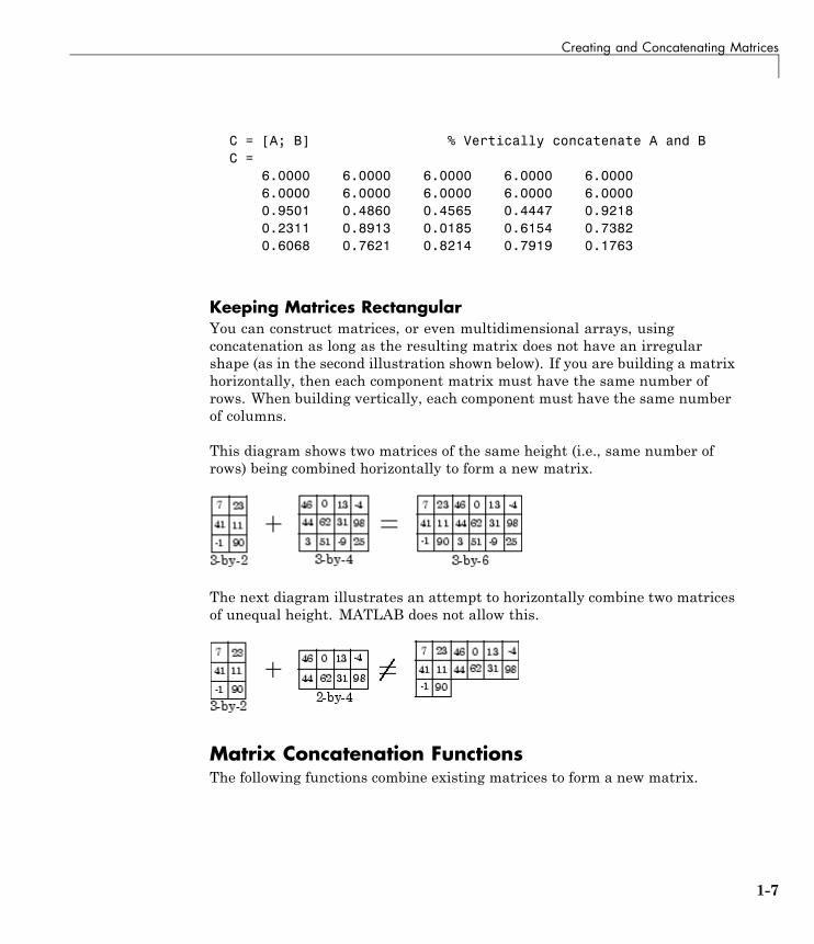
C = [A; B] % Vertically concatenate A and BC =
6.0000 6.0000 6.0000 6.0000 6.00006.0000 6.0000 6.0000 6.0000 6.00000.9501 0.4860 0.4565 0.4447 0.92180.2311 0.8913 0.0185 0.6154 0.73820.6068 0.7621 0.8214 0.7919 0.1763
Keeping Matrices RectangularYou can construct matrices, or even multidimensional arrays, usingconcatenation as long as the resulting matrix does not have an irregularshape (as in the second illustration shown below). If you are building a matrixhorizontally, then each component matrix must have the same number ofrows. When building vertically, each component must have the same numberof columns.
This diagram shows two matrices of the same height (i.e., same number ofrows) being combined horizontally to form a new matrix.
The next diagram illustrates an attempt to horizontally combine two matricesof unequal height. MATLAB does not allow this.
Matrix Concatenation FunctionsThe following functions combine existing matrices to form a new matrix.
1-7
1 Matrices and Arrays
Function Description
cat Concatenate matrices along the specified dimension
horzcat Horizontally concatenate matrices
vertcat Vertically concatenate matrices
repmat Create a new matrix by replicating and tiling existingmatrices
blkdiag Create a block diagonal matrix from existing matrices
ExamplesHere are some examples of how you can use these functions.
Concatenating Matrices and Arrays. An alternative to using the []operator for concatenation are the three functions cat, horzcat, and vertcat.With these functions, you can construct matrices (or multidimensional arrays)along a specified dimension. Either of the following commands accomplish thesame task as the command C = [A; B] used in the section on “ConcatenatingMatrices” on page 1-6:
C = cat(1, A, B); % Concatenate along the first dimensionC = vertcat(A, B); % Concatenate vertically
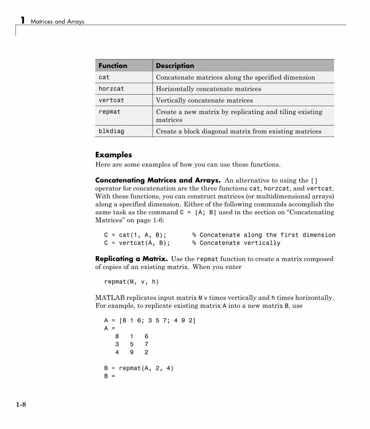
Replicating a Matrix. Use the repmat function to create a matrix composedof copies of an existing matrix. When you enter
repmat(M, v, h)
MATLAB replicates input matrix M v times vertically and h times horizontally.For example, to replicate existing matrix A into a new matrix B, use
A = [8 1 6; 3 5 7; 4 9 2]A =
8 1 63 5 74 9 2
B = repmat(A, 2, 4)B =
1-8
Creating and Concatenating Matrices
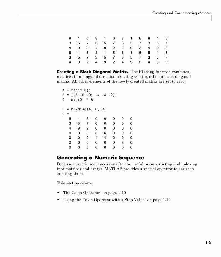
8 1 6 8 1 6 8 1 6 8 1 63 5 7 3 5 7 3 5 7 3 5 74 9 2 4 9 2 4 9 2 4 9 28 1 6 8 1 6 8 1 6 8 1 63 5 7 3 5 7 3 5 7 3 5 74 9 2 4 9 2 4 9 2 4 9 2
Creating a Block Diagonal Matrix. The blkdiag function combinesmatrices in a diagonal direction, creating what is called a block diagonalmatrix. All other elements of the newly created matrix are set to zero:
A = magic(3);B = [-5 -6 -9; -4 -4 -2];C = eye(2) * 8;
D = blkdiag(A, B, C)D =
8 1 6 0 0 0 0 03 5 7 0 0 0 0 04 9 2 0 0 0 0 00 0 0 -5 -6 -9 0 00 0 0 -4 -4 -2 0 00 0 0 0 0 0 8 00 0 0 0 0 0 0 8
Generating a Numeric SequenceBecause numeric sequences can often be useful in constructing and indexinginto matrices and arrays, MATLAB provides a special operator to assist increating them.
This section covers
• “The Colon Operator” on page 1-10
• “Using the Colon Operator with a Step Value” on page 1-10
1-9
1 Matrices and Arrays
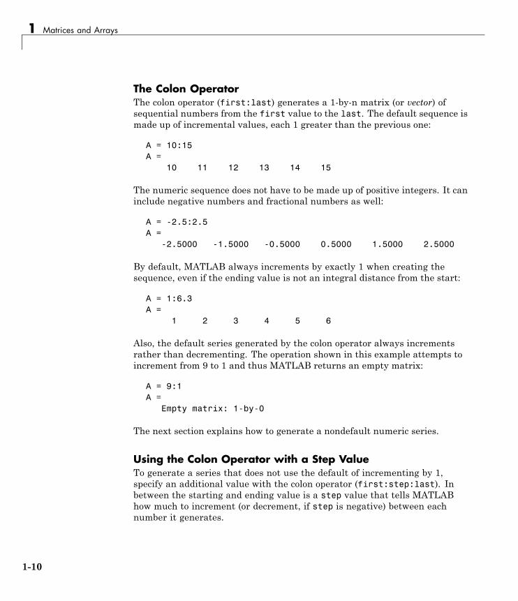
The Colon OperatorThe colon operator (first:last) generates a 1-by-n matrix (or vector) ofsequential numbers from the first value to the last. The default sequence ismade up of incremental values, each 1 greater than the previous one:
A = 10:15A =
10 11 12 13 14 15
The numeric sequence does not have to be made up of positive integers. It caninclude negative numbers and fractional numbers as well:
A = -2.5:2.5A =
-2.5000 -1.5000 -0.5000 0.5000 1.5000 2.5000
By default, MATLAB always increments by exactly 1 when creating thesequence, even if the ending value is not an integral distance from the start:
A = 1:6.3A =
1 2 3 4 5 6
Also, the default series generated by the colon operator always incrementsrather than decrementing. The operation shown in this example attempts toincrement from 9 to 1 and thus MATLAB returns an empty matrix:
A = 9:1A =
Empty matrix: 1-by-0
The next section explains how to generate a nondefault numeric series.
Using the Colon Operator with a Step ValueTo generate a series that does not use the default of incrementing by 1,specify an additional value with the colon operator (first:step:last). Inbetween the starting and ending value is a step value that tells MATLABhow much to increment (or decrement, if step is negative) between eachnumber it generates.
1-10
Creating and Concatenating Matrices
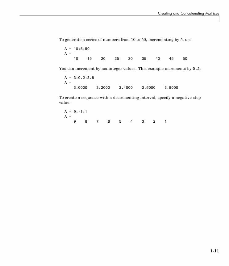
To generate a series of numbers from 10 to 50, incrementing by 5, use
A = 10:5:50A =
10 15 20 25 30 35 40 45 50
You can increment by noninteger values. This example increments by 0.2:
A = 3:0.2:3.8A =
3.0000 3.2000 3.4000 3.6000 3.8000
To create a sequence with a decrementing interval, specify a negative stepvalue:
A = 9:-1:1A =
9 8 7 6 5 4 3 2 1
1-11
1 Matrices and Arrays
Matrix Indexing
In this section...
“Accessing Single Elements” on page 1-12
“Linear Indexing” on page 1-13
“Functions That Control Indexing Style” on page 1-13
“Accessing Multiple Elements” on page 1-14
“Using Logicals in Array Indexing” on page 1-17
“Single-Colon Indexing with Different Array Types” on page 1-20
“Indexing on Assignment” on page 1-21
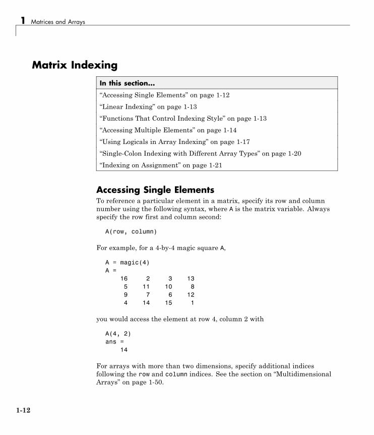
Accessing Single ElementsTo reference a particular element in a matrix, specify its row and columnnumber using the following syntax, where A is the matrix variable. Alwaysspecify the row first and column second:
A(row, column)
For example, for a 4-by-4 magic square A,
A = magic(4)A =
16 2 3 135 11 10 89 7 6 124 14 15 1
you would access the element at row 4, column 2 with
A(4, 2)ans =
14
For arrays with more than two dimensions, specify additional indicesfollowing the row and column indices. See the section on “MultidimensionalArrays” on page 1-50.
1-12
Matrix Indexing
Linear IndexingYou can refer to the elements of a MATLAB matrix with a single subscript,A(k). MATLAB stores matrices and arrays not in the shape that they appearwhen displayed in the MATLAB Command Window, but as a single columnof elements. This single column is composed of all of the columns from thematrix, each appended to the last.
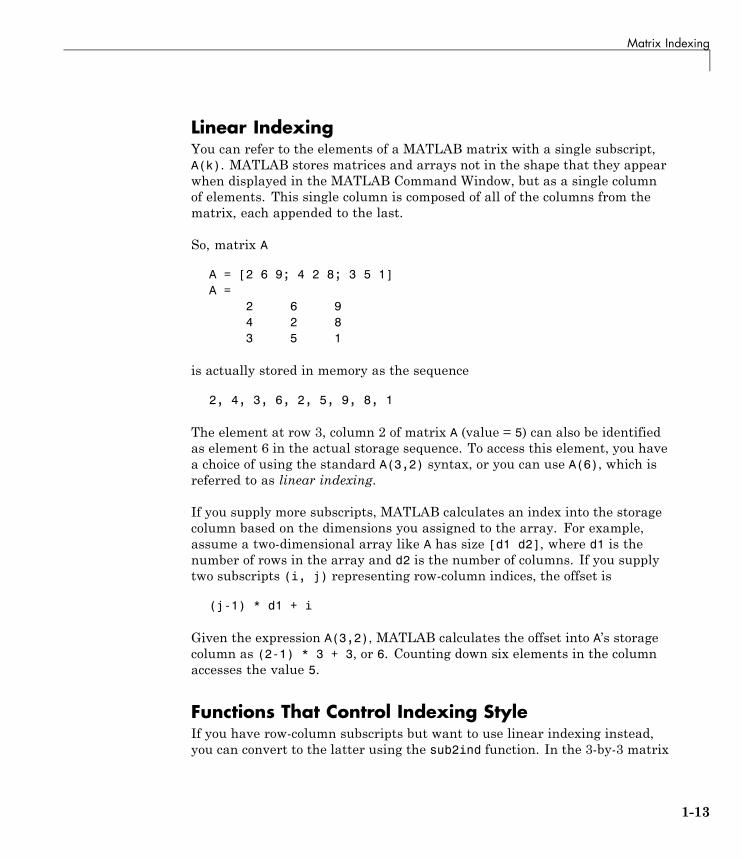
So, matrix A
A = [2 6 9; 4 2 8; 3 5 1]A =
2 6 94 2 83 5 1
is actually stored in memory as the sequence
2, 4, 3, 6, 2, 5, 9, 8, 1
The element at row 3, column 2 of matrix A (value = 5) can also be identifiedas element 6 in the actual storage sequence. To access this element, you havea choice of using the standard A(3,2) syntax, or you can use A(6), which isreferred to as linear indexing.
If you supply more subscripts, MATLAB calculates an index into the storagecolumn based on the dimensions you assigned to the array. For example,assume a two-dimensional array like A has size [d1 d2], where d1 is thenumber of rows in the array and d2 is the number of columns. If you supplytwo subscripts (i, j) representing row-column indices, the offset is
(j-1) * d1 + i
Given the expression A(3,2), MATLAB calculates the offset into A’s storagecolumn as (2-1) * 3 + 3, or 6. Counting down six elements in the columnaccesses the value 5.
Functions That Control Indexing StyleIf you have row-column subscripts but want to use linear indexing instead,you can convert to the latter using the sub2ind function. In the 3-by-3 matrix
1-13
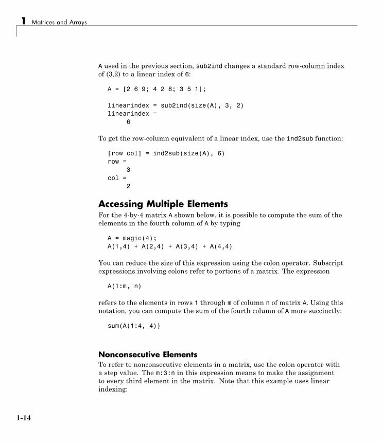
1 Matrices and Arrays
A used in the previous section, sub2ind changes a standard row-column indexof (3,2) to a linear index of 6:
A = [2 6 9; 4 2 8; 3 5 1];
linearindex = sub2ind(size(A), 3, 2)linearindex =
6
To get the row-column equivalent of a linear index, use the ind2sub function:
[row col] = ind2sub(size(A), 6)row =
3col =
2
Accessing Multiple ElementsFor the 4-by-4 matrix A shown below, it is possible to compute the sum of theelements in the fourth column of A by typing
A = magic(4);A(1,4) + A(2,4) + A(3,4) + A(4,4)
You can reduce the size of this expression using the colon operator. Subscriptexpressions involving colons refer to portions of a matrix. The expression
A(1:m, n)
refers to the elements in rows 1 through m of column n of matrix A. Using thisnotation, you can compute the sum of the fourth column of A more succinctly:
sum(A(1:4, 4))
Nonconsecutive ElementsTo refer to nonconsecutive elements in a matrix, use the colon operator witha step value. The m:3:n in this expression means to make the assignmentto every third element in the matrix. Note that this example uses linearindexing:
1-14
Matrix Indexing
B = A;
B(1:3:16) = -10B =
-10 2 3 -105 11 -10 89 -10 6 12
-10 14 15 -10
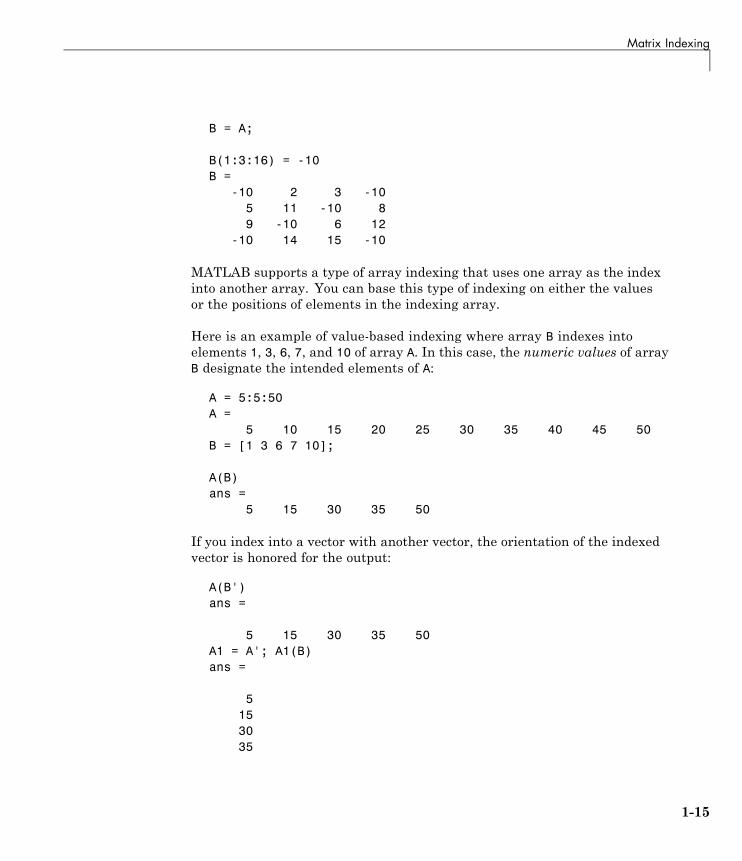
MATLAB supports a type of array indexing that uses one array as the indexinto another array. You can base this type of indexing on either the valuesor the positions of elements in the indexing array.
Here is an example of value-based indexing where array B indexes intoelements 1, 3, 6, 7, and 10 of array A. In this case, the numeric values of arrayB designate the intended elements of A:
A = 5:5:50A =
5 10 15 20 25 30 35 40 45 50B = [1 3 6 7 10];
A(B)ans =
5 15 30 35 50
If you index into a vector with another vector, the orientation of the indexedvector is honored for the output:
A(B')ans =
5 15 30 35 50A1 = A'; A1(B)ans =
5153035
1-15
1 Matrices and Arrays
50
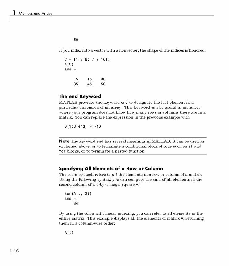
If you index into a vector with a nonvector, the shape of the indices is honored.:
C = [1 3 6; 7 9 10];A(C)ans =
5 15 3035 45 50
The end KeywordMATLAB provides the keyword end to designate the last element in aparticular dimension of an array. This keyword can be useful in instanceswhere your program does not know how many rows or columns there are in amatrix. You can replace the expression in the previous example with
B(1:3:end) = -10
Note The keyword end has several meanings in MATLAB. It can be used asexplained above, or to terminate a conditional block of code such as if andfor blocks, or to terminate a nested function.
Specifying All Elements of a Row or ColumnThe colon by itself refers to all the elements in a row or column of a matrix.Using the following syntax, you can compute the sum of all elements in thesecond column of a 4-by-4 magic square A:
sum(A(:, 2))ans =
34
By using the colon with linear indexing, you can refer to all elements in theentire matrix. This example displays all the elements of matrix A, returningthem in a column-wise order:
A(:)
1-16
Matrix Indexing
ans =16594...
121
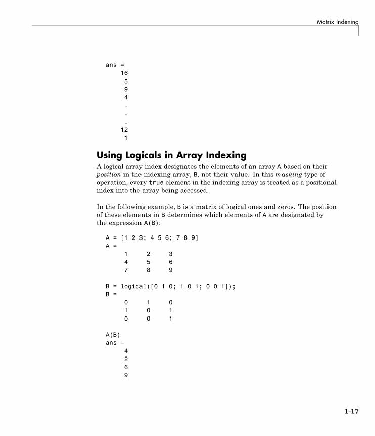
Using Logicals in Array IndexingA logical array index designates the elements of an array A based on theirposition in the indexing array, B, not their value. In this masking type ofoperation, every true element in the indexing array is treated as a positionalindex into the array being accessed.
In the following example, B is a matrix of logical ones and zeros. The positionof these elements in B determines which elements of A are designated bythe expression A(B):
A = [1 2 3; 4 5 6; 7 8 9]A =
1 2 34 5 67 8 9
B = logical([0 1 0; 1 0 1; 0 0 1]);B =
0 1 01 0 10 0 1
A(B)ans =
4269
1-17
1 Matrices and Arrays
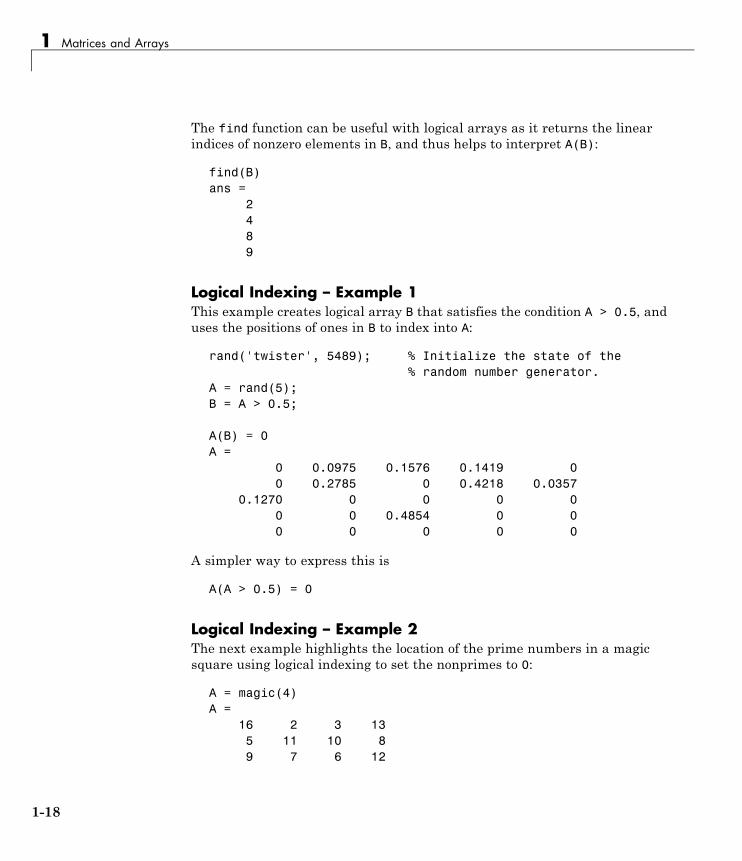
The find function can be useful with logical arrays as it returns the linearindices of nonzero elements in B, and thus helps to interpret A(B):
find(B)ans =
2489
Logical Indexing – Example 1This example creates logical array B that satisfies the condition A > 0.5, anduses the positions of ones in B to index into A:
rand('twister', 5489); % Initialize the state of the% random number generator.
A = rand(5);B = A > 0.5;
A(B) = 0A =
0 0.0975 0.1576 0.1419 00 0.2785 0 0.4218 0.0357
0.1270 0 0 0 00 0 0.4854 0 00 0 0 0 0
A simpler way to express this is
A(A > 0.5) = 0
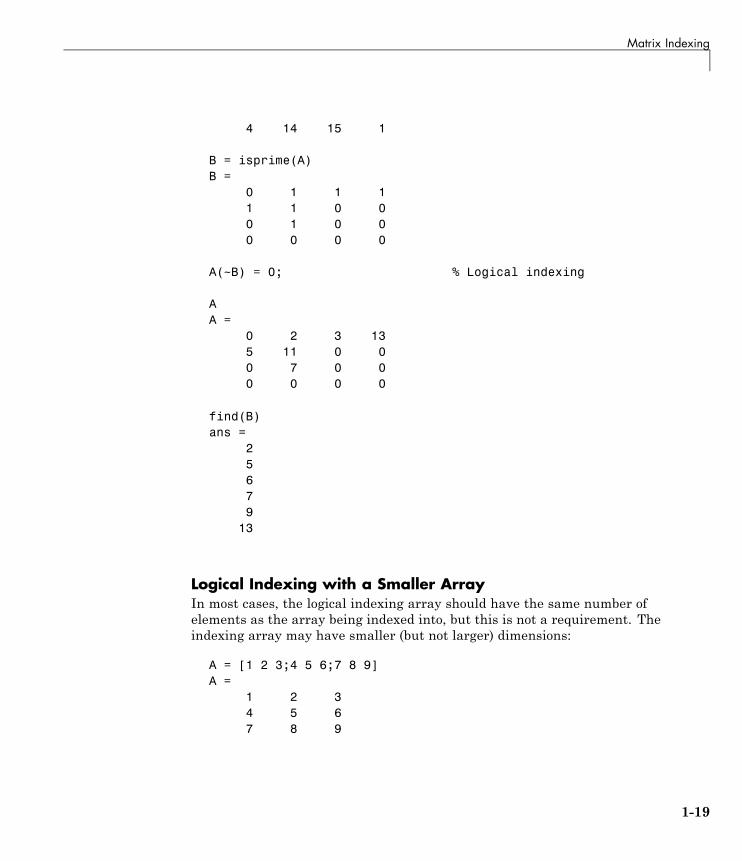
Logical Indexing – Example 2The next example highlights the location of the prime numbers in a magicsquare using logical indexing to set the nonprimes to 0:
A = magic(4)A =
16 2 3 135 11 10 89 7 6 12
1-18
Matrix Indexing
4 14 15 1
B = isprime(A)B =
0 1 1 11 1 0 00 1 0 00 0 0 0
A(~B) = 0; % Logical indexing
AA =
0 2 3 135 11 0 00 7 0 00 0 0 0
find(B)ans =
25679
13
Logical Indexing with a Smaller ArrayIn most cases, the logical indexing array should have the same number ofelements as the array being indexed into, but this is not a requirement. Theindexing array may have smaller (but not larger) dimensions:
A = [1 2 3;4 5 6;7 8 9]A =
1 2 34 5 67 8 9
1-19
1 Matrices and Arrays
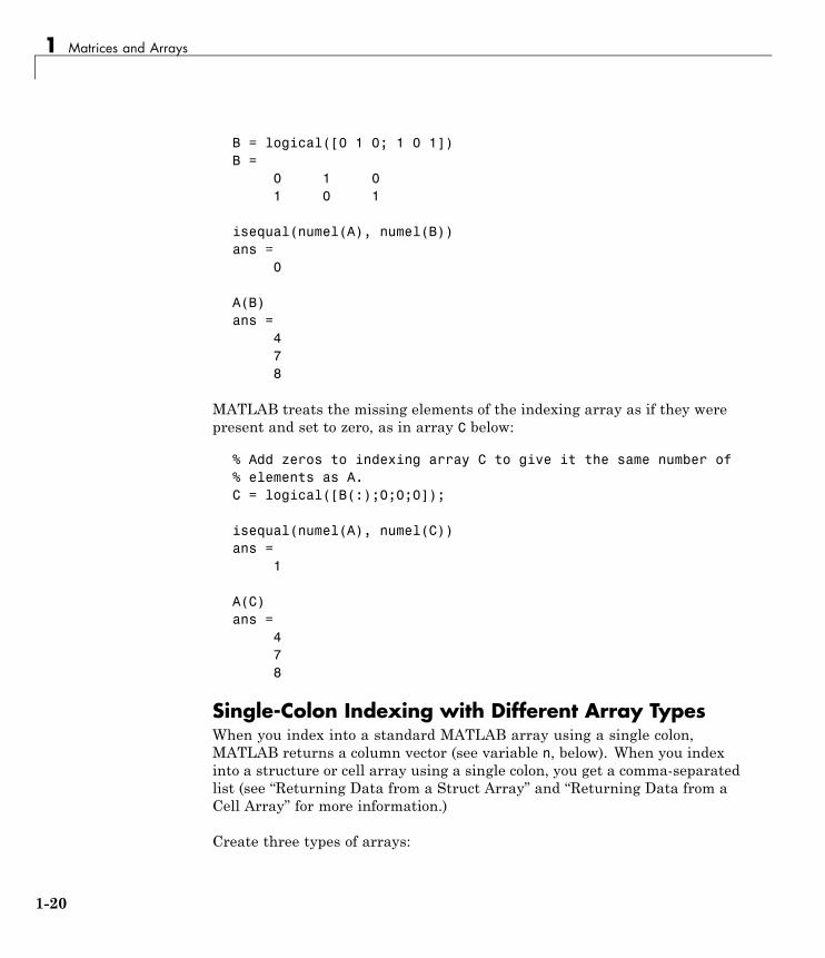
B = logical([0 1 0; 1 0 1])B =
0 1 01 0 1
isequal(numel(A), numel(B))ans =
0
A(B)ans =
478
MATLAB treats the missing elements of the indexing array as if they werepresent and set to zero, as in array C below:
% Add zeros to indexing array C to give it the same number of% elements as A.C = logical([B(:);0;0;0]);
isequal(numel(A), numel(C))ans =
1
A(C)ans =
478
Single-Colon Indexing with Different Array TypesWhen you index into a standard MATLAB array using a single colon,MATLAB returns a column vector (see variable n, below). When you indexinto a structure or cell array using a single colon, you get a comma-separatedlist (see “Returning Data from a Struct Array” and “Returning Data from aCell Array” for more information.)
Create three types of arrays:
1-20
Matrix Indexing
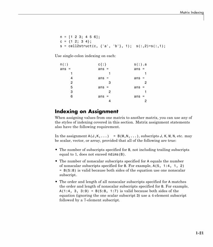
n = [1 2 3; 4 5 6];c = {1 2; 3 4};s = cell2struct(c, {'a', 'b'}, 1); s(:,2)=s(:,1);
Use single-colon indexing on each:
n(:) c{:} s(:).aans = ans = ans =
1 1 14 ans = ans =2 3 25 ans = ans =3 2 16 ans = ans =
4 2
Indexing on AssignmentWhen assigning values from one matrix to another matrix, you can use any ofthe styles of indexing covered in this section. Matrix assignment statementsalso have the following requirement.
In the assignment A(J,K,...) = B(M,N,...), subscripts J, K, M, N, etc. maybe scalar, vector, or array, provided that all of the following are true:
• The number of subscripts specified for B, not including trailing subscriptsequal to 1, does not exceed ndims(B).
• The number of nonscalar subscripts specified for A equals the numberof nonscalar subscripts specified for B. For example, A(5, 1:4, 1, 2)= B(5:8) is valid because both sides of the equation use one nonscalarsubscript.
• The order and length of all nonscalar subscripts specified for A matchesthe order and length of nonscalar subscripts specified for B. For example,A(1:4, 3, 3:9) = B(5:8, 1:7) is valid because both sides of theequation (ignoring the one scalar subscript 3) use a 4-element subscriptfollowed by a 7-element subscript.
1-21
1 Matrices and Arrays
Getting Information About a Matrix
In this section...
“Dimensions of the Matrix” on page 1-22
“Classes Used in the Matrix” on page 1-23
“Data Structures Used in the Matrix” on page 1-24
Dimensions of the MatrixThese functions return information about the shape and size of a matrix.
Function Description
length Return the length of the longest dimension. (The length of amatrix or array with any zero dimension is zero.)
ndims Return the number of dimensions.
numel Return the number of elements.
size Return the length of each dimension.
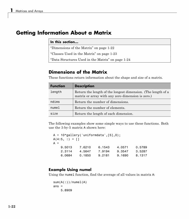
The following examples show some simple ways to use these functions. Bothuse the 3-by-5 matrix A shown here:
A = 10*gallery('uniformdata',[5],0);A(4:5, :) = []A =
9.5013 7.6210 6.1543 4.0571 0.57892.3114 4.5647 7.9194 9.3547 3.52876.0684 0.1850 9.2181 9.1690 8.1317
Example Using numelUsing the numel function, find the average of all values in matrix A:
sum(A(:))/numel(A)ans =
5.8909
1-22
Getting Information About a Matrix
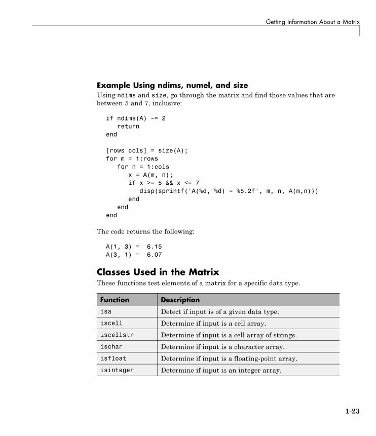
Example Using ndims, numel, and sizeUsing ndims and size, go through the matrix and find those values that arebetween 5 and 7, inclusive:
if ndims(A) ~= 2return
end
[rows cols] = size(A);for m = 1:rows
for n = 1:colsx = A(m, n);if x >= 5 && x <= 7
disp(sprintf('A(%d, %d) = %5.2f', m, n, A(m,n)))end
endend
The code returns the following:
A(1, 3) = 6.15A(3, 1) = 6.07
Classes Used in the MatrixThese functions test elements of a matrix for a specific data type.
Function Description
isa Detect if input is of a given data type.
iscell Determine if input is a cell array.
iscellstr Determine if input is a cell array of strings.
ischar Determine if input is a character array.
isfloat Determine if input is a floating-point array.
isinteger Determine if input is an integer array.
1-23
1 Matrices and Arrays
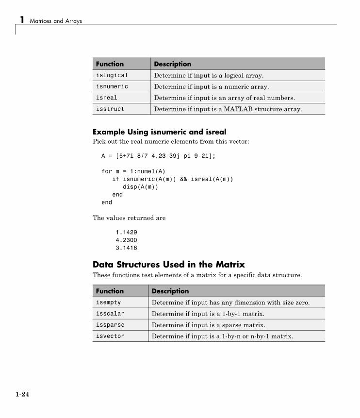
Function Description
islogical Determine if input is a logical array.
isnumeric Determine if input is a numeric array.
isreal Determine if input is an array of real numbers.
isstruct Determine if input is a MATLAB structure array.
Example Using isnumeric and isrealPick out the real numeric elements from this vector:
A = [5+7i 8/7 4.23 39j pi 9-2i];
for m = 1:numel(A)if isnumeric(A(m)) && isreal(A(m))
disp(A(m))end
end
The values returned are
1.14294.23003.1416
Data Structures Used in the MatrixThese functions test elements of a matrix for a specific data structure.
Function Description
isempty Determine if input has any dimension with size zero.
isscalar Determine if input is a 1-by-1 matrix.
issparse Determine if input is a sparse matrix.
isvector Determine if input is a 1-by-n or n-by-1 matrix.
1-24
Resizing and Reshaping Matrices
Resizing and Reshaping Matrices
In this section...
“Expanding the Size of a Matrix” on page 1-25
“Diminishing the Size of a Matrix” on page 1-29
“Reshaping a Matrix” on page 1-30
“Preallocating Memory” on page 1-32
Expanding the Size of a MatrixYou can expand the size of any existing matrix as long as doing so doesnot give the resulting matrix an irregular shape. (See “Keeping MatricesRectangular” on page 1-7). For example, you can vertically combine a 4-by-3matrix and 7-by-3 matrix because all rows of the resulting matrix have thesame number of columns (3).
Two ways of expanding the size of an existing matrix are
• Concatenating new elements onto the matrix
• Storing to a location outside the bounds of the matrix
Note If you intend to expand the size of a matrix repeatedly over timeas it requires more room (usually done in a programming loop), it isadvisable to preallocate space for the matrix when you initially create it. See“Preallocating Memory” on page 1-32.
Concatenating Onto the MatrixConcatenation is most useful when you want to expand a matrix by addingnew elements or blocks that are compatible in size with the original matrix.This means that the size of all matrices being joined along a specific dimensionmust be equal along that dimension. See “Concatenating Matrices” on page1-6.
1-25
1 Matrices and Arrays
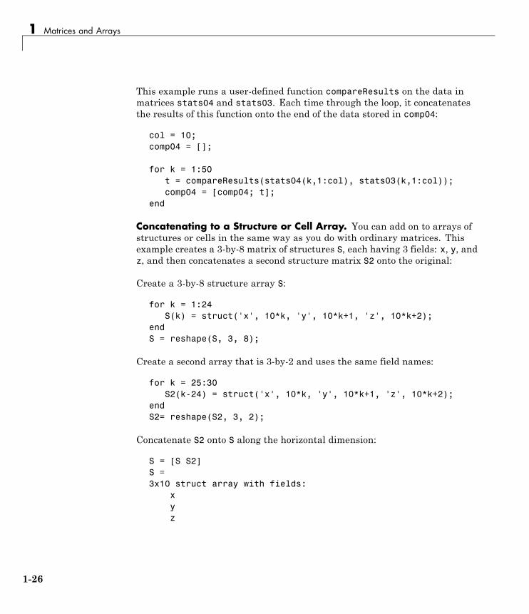
This example runs a user-defined function compareResults on the data inmatrices stats04 and stats03. Each time through the loop, it concatenatesthe results of this function onto the end of the data stored in comp04:
col = 10;comp04 = [];
for k = 1:50t = compareResults(stats04(k,1:col), stats03(k,1:col));comp04 = [comp04; t];
end
Concatenating to a Structure or Cell Array. You can add on to arrays ofstructures or cells in the same way as you do with ordinary matrices. Thisexample creates a 3-by-8 matrix of structures S, each having 3 fields: x, y, andz, and then concatenates a second structure matrix S2 onto the original:
Create a 3-by-8 structure array S:
for k = 1:24S(k) = struct('x', 10*k, 'y', 10*k+1, 'z', 10*k+2);
endS = reshape(S, 3, 8);
Create a second array that is 3-by-2 and uses the same field names:
for k = 25:30S2(k-24) = struct('x', 10*k, 'y', 10*k+1, 'z', 10*k+2);
endS2= reshape(S2, 3, 2);
Concatenate S2 onto S along the horizontal dimension:
S = [S S2]S =3x10 struct array with fields:
xyz
1-26
Resizing and Reshaping Matrices
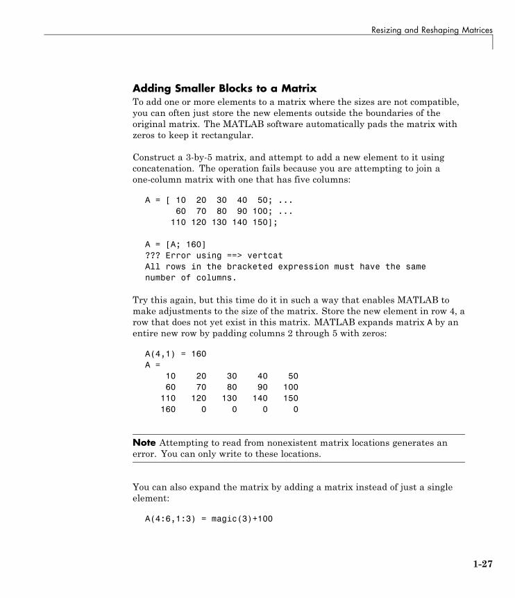
Adding Smaller Blocks to a MatrixTo add one or more elements to a matrix where the sizes are not compatible,you can often just store the new elements outside the boundaries of theoriginal matrix. The MATLAB software automatically pads the matrix withzeros to keep it rectangular.
Construct a 3-by-5 matrix, and attempt to add a new element to it usingconcatenation. The operation fails because you are attempting to join aone-column matrix with one that has five columns:
A = [ 10 20 30 40 50; ...60 70 80 90 100; ...
110 120 130 140 150];
A = [A; 160]??? Error using ==> vertcatAll rows in the bracketed expression must have the samenumber of columns.
Try this again, but this time do it in such a way that enables MATLAB tomake adjustments to the size of the matrix. Store the new element in row 4, arow that does not yet exist in this matrix. MATLAB expands matrix A by anentire new row by padding columns 2 through 5 with zeros:
A(4,1) = 160A =
10 20 30 40 5060 70 80 90 100
110 120 130 140 150160 0 0 0 0
Note Attempting to read from nonexistent matrix locations generates anerror. You can only write to these locations.
You can also expand the matrix by adding a matrix instead of just a singleelement:
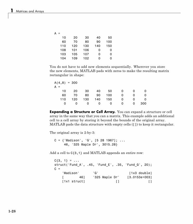
A(4:6,1:3) = magic(3)+100
1-27
1 Matrices and Arrays
A =10 20 30 40 5060 70 80 90 100
110 120 130 140 150108 101 106 0 0103 105 107 0 0104 109 102 0 0
You do not have to add new elements sequentially. Wherever you storethe new elements, MATLAB pads with zeros to make the resulting matrixrectangular in shape:
A(4,8) = 300A =
10 20 30 40 50 0 0 060 70 80 90 100 0 0 0
110 120 130 140 150 0 0 00 0 0 0 0 0 0 300
Expanding a Structure or Cell Array. You can expand a structure or cellarray in the same way that you can a matrix. This example adds an additionalcell to a cell array by storing it beyond the bounds of the original array.MATLAB pads the data structure with empty cells ([]) to keep it rectangular.
The original array is 2-by-3:
C = {'Madison', 'G', [5 28 1967]; ...46, '325 Maple Dr', 3015.28}
Add a cell to C{3,1} and MATLAB appends an entire row:
C{3, 1} = ...struct('Fund_A', .45, 'Fund_E', .35, 'Fund_G', 20);C =
'Madison' 'G' [1x3 double][ 46] '325 Maple Dr' [3.0153e+003][1x1 struct] [] []
1-28
Resizing and Reshaping Matrices
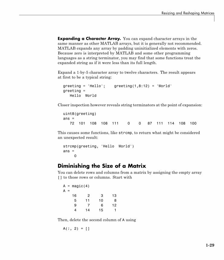
Expanding a Character Array. You can expand character arrays in thesame manner as other MATLAB arrays, but it is generally not recommended.MATLAB expands any array by padding uninitialized elements with zeros.Because zero is interpreted by MATLAB and some other programminglanguages as a string terminator, you may find that some functions treat theexpanded string as if it were less than its full length.
Expand a 1-by-5 character array to twelve characters. The result appearsat first to be a typical string:
greeting = 'Hello'; greeting(1,8:12) = 'World'greeting =
Hello World
Closer inspection however reveals string terminators at the point of expansion:
uint8(greeting)ans =
72 101 108 108 111 0 0 87 111 114 108 100
This causes some functions, like strcmp, to return what might be consideredan unexpected result:
strcmp(greeting, 'Hello World')ans =
0
Diminishing the Size of a MatrixYou can delete rows and columns from a matrix by assigning the empty array[] to those rows or columns. Start with
A = magic(4)A =
16 2 3 135 11 10 89 7 6 124 14 15 1
Then, delete the second column of A using
A(:, 2) = []
1-29
1 Matrices and Arrays
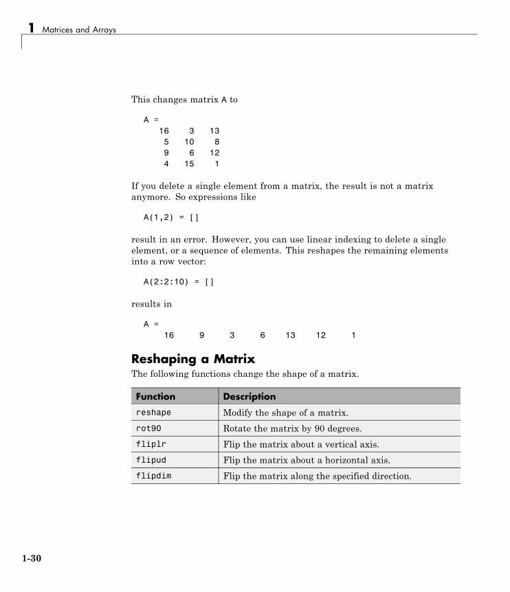
This changes matrix A to
A =16 3 135 10 89 6 124 15 1
If you delete a single element from a matrix, the result is not a matrixanymore. So expressions like
A(1,2) = []
result in an error. However, you can use linear indexing to delete a singleelement, or a sequence of elements. This reshapes the remaining elementsinto a row vector:
A(2:2:10) = []
results in
A =16 9 3 6 13 12 1
Reshaping a MatrixThe following functions change the shape of a matrix.
Function Description
reshape Modify the shape of a matrix.
rot90 Rotate the matrix by 90 degrees.
fliplr Flip the matrix about a vertical axis.
flipud Flip the matrix about a horizontal axis.
flipdim Flip the matrix along the specified direction.
1-30
Resizing and Reshaping Matrices
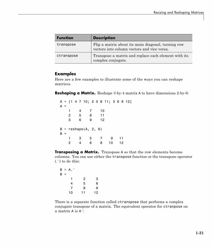
Function Description
transpose Flip a matrix about its main diagonal, turning rowvectors into column vectors and vice versa.
ctranspose Transpose a matrix and replace each element with itscomplex conjugate.
ExamplesHere are a few examples to illustrate some of the ways you can reshapematrices.
Reshaping a Matrix. Reshape 3-by-4 matrix A to have dimensions 2-by-6:
A = [1 4 7 10; 2 5 8 11; 3 6 9 12]A =
1 4 7 102 5 8 113 6 9 12
B = reshape(A, 2, 6)B =
1 3 5 7 9 112 4 6 8 10 12
Transposing a Matrix. Transpose A so that the row elements becomecolumns. You can use either the transpose function or the transpose operator(.') to do this:
B = A.'B =
1 2 34 5 67 8 9
10 11 12
There is a separate function called ctranspose that performs a complexconjugate transpose of a matrix. The equivalent operator for ctranpose ona matrix A is A':
1-31
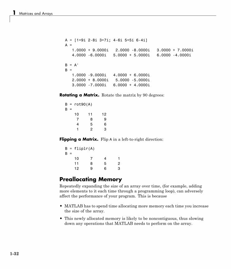
1 Matrices and Arrays
A = [1+9i 2-8i 3+7i; 4-6i 5+5i 6-4i]A =
1.0000 + 9.0000i 2.0000 -8.0000i 3.0000 + 7.0000i4.0000 -6.0000i 5.0000 + 5.0000i 6.0000 -4.0000i
B = A'B =
1.0000 -9.0000i 4.0000 + 6.0000i2.0000 + 8.0000i 5.0000 -5.0000i3.0000 -7.0000i 6.0000 + 4.0000i
Rotating a Matrix. Rotate the matrix by 90 degrees:
B = rot90(A)B =
10 11 127 8 94 5 61 2 3
Flipping a Matrix. Flip A in a left-to-right direction:
B = fliplr(A)B =
10 7 4 111 8 5 212 9 6 3
Preallocating MemoryRepeatedly expanding the size of an array over time, (for example, addingmore elements to it each time through a programming loop), can adverselyaffect the performance of your program. This is because
• MATLAB has to spend time allocating more memory each time you increasethe size of the array.
• This newly allocated memory is likely to be noncontiguous, thus slowingdown any operations that MATLAB needs to perform on the array.
1-32
Resizing and Reshaping Matrices
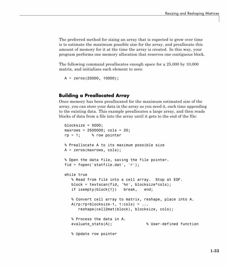
The preferred method for sizing an array that is expected to grow over timeis to estimate the maximum possible size for the array, and preallocate thisamount of memory for it at the time the array is created. In this way, yourprogram performs one memory allocation that reserves one contiguous block.
The following command preallocates enough space for a 25,000 by 10,000matrix, and initializes each element to zero:
A = zeros(25000, 10000);
Building a Preallocated ArrayOnce memory has been preallocated for the maximum estimated size of thearray, you can store your data in the array as you need it, each time appendingto the existing data. This example preallocates a large array, and then readsblocks of data from a file into the array until it gets to the end of the file:
blocksize = 5000;maxrows = 2500000; cols = 20;rp = 1; % row pointer
% Preallocate A to its maximum possible sizeA = zeros(maxrows, cols);
% Open the data file, saving the file pointer.fid = fopen('statfile.dat', 'r');
while true% Read from file into a cell array. Stop at EOF.block = textscan(fid, '%n', blocksize*cols);if isempty(block{1}) break, end;
% Convert cell array to matrix, reshape, place into A.A(rp:rp+blocksize-1, 1:cols) = ...
reshape(cell2mat(block), blocksize, cols);
% Process the data in A.evaluate_stats(A); % User-defined function
% Update row pointer
1-33
1 Matrices and Arrays
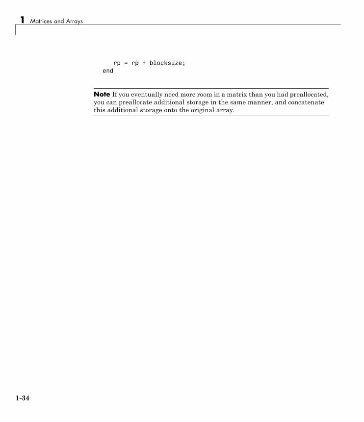
rp = rp + blocksize;end
Note If you eventually need more room in a matrix than you had preallocated,you can preallocate additional storage in the same manner, and concatenatethis additional storage onto the original array.
1-34
Shifting and Sorting Matrices
Shifting and Sorting Matrices
In this section...
“Shift and Sort Functions” on page 1-35
“Shifting the Location of Matrix Elements” on page 1-35
“Sorting the Data in Each Column” on page 1-37
“Sorting the Data in Each Row” on page 1-37
“Sorting Row Vectors” on page 1-38
Shift and Sort FunctionsUse these functions to shift or sort the elements of a matrix.
Function Description
circshift Circularly shift matrix contents.
sort Sort array elements in ascending or descending order.
sortrows Sort rows in ascending order.
issorted Determine if matrix elements are in sorted order.
You can sort matrices, multidimensional arrays, and cell arrays of stringsalong any dimension and in ascending or descending order of the elements.The sort functions also return an optional array of indices showing the orderin which elements were rearranged during the sorting operation.
Shifting the Location of Matrix ElementsThe circshift function shifts the elements of a matrix in a circular manneralong one or more dimensions. Rows or columns that are shifted out of thematrix circulate back into the opposite end. For example, shifting a 4-by-7matrix one place to the left moves the elements in columns 2 through 7 tocolumns 1 through 6, and moves column 1 to column 7.
Create a 5-by-8 matrix named A and shift it to the right along the second(horizontal) dimension by three places. (You would use [0, -3] to shift to theleft by three places):
1-35
1 Matrices and Arrays
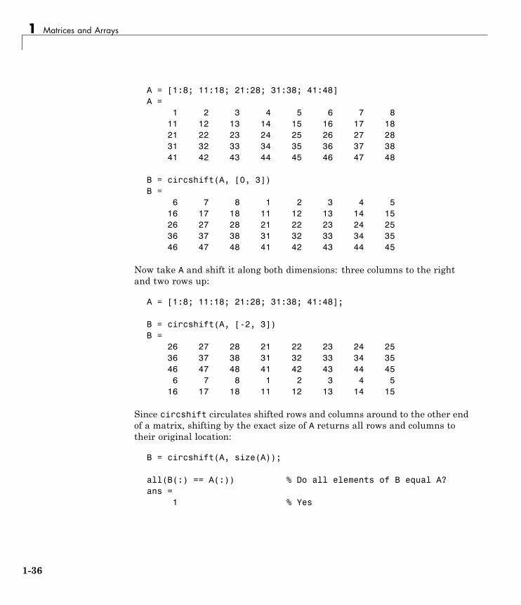
A = [1:8; 11:18; 21:28; 31:38; 41:48]A =
1 2 3 4 5 6 7 811 12 13 14 15 16 17 1821 22 23 24 25 26 27 2831 32 33 34 35 36 37 3841 42 43 44 45 46 47 48
B = circshift(A, [0, 3])B =
6 7 8 1 2 3 4 516 17 18 11 12 13 14 1526 27 28 21 22 23 24 2536 37 38 31 32 33 34 3546 47 48 41 42 43 44 45
Now take A and shift it along both dimensions: three columns to the rightand two rows up:
A = [1:8; 11:18; 21:28; 31:38; 41:48];
B = circshift(A, [-2, 3])B =
26 27 28 21 22 23 24 2536 37 38 31 32 33 34 3546 47 48 41 42 43 44 456 7 8 1 2 3 4 5
16 17 18 11 12 13 14 15
Since circshift circulates shifted rows and columns around to the other endof a matrix, shifting by the exact size of A returns all rows and columns totheir original location:
B = circshift(A, size(A));
all(B(:) == A(:)) % Do all elements of B equal A?ans =
1 % Yes
1-36
Shifting and Sorting Matrices
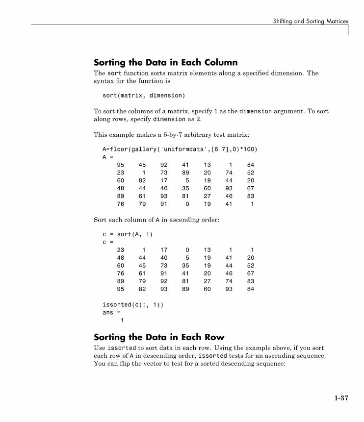
Sorting the Data in Each ColumnThe sort function sorts matrix elements along a specified dimension. Thesyntax for the function is
sort(matrix, dimension)
To sort the columns of a matrix, specify 1 as the dimension argument. To sortalong rows, specify dimension as 2.
This example makes a 6-by-7 arbitrary test matrix:
A=floor(gallery('uniformdata',[6 7],0)*100)A =
95 45 92 41 13 1 8423 1 73 89 20 74 5260 82 17 5 19 44 2048 44 40 35 60 93 6789 61 93 81 27 46 8376 79 91 0 19 41 1
Sort each column of A in ascending order:
c = sort(A, 1)c =
23 1 17 0 13 1 148 44 40 5 19 41 2060 45 73 35 19 44 5276 61 91 41 20 46 6789 79 92 81 27 74 8395 82 93 89 60 93 84
issorted(c(:, 1))ans =
1
Sorting the Data in Each RowUse issorted to sort data in each row. Using the example above, if you sorteach row of A in descending order, issorted tests for an ascending sequence.You can flip the vector to test for a sorted descending sequence:
1-37
1 Matrices and Arrays
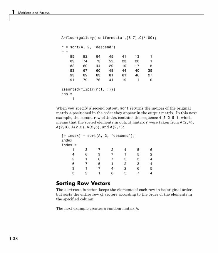
A=floor(gallery('uniformdata',[6 7],0)*100);
r = sort(A, 2, 'descend')r =
95 92 84 45 41 13 189 74 73 52 23 20 182 60 44 20 19 17 593 67 60 48 44 40 3593 89 83 81 61 46 2791 79 76 41 19 1 0
issorted(fliplr(r(1, :)))ans =
1
When you specify a second output, sort returns the indices of the originalmatrix A positioned in the order they appear in the output matrix. In this nextexample, the second row of index contains the sequence 4 3 2 5 1, whichmeans that the sorted elements in output matrix r were taken from A(2,4),A(2,3), A(2,2), A(2,5), and A(2,1):
[r index] = sort(A, 2, 'descend');indexindex =
1 3 7 2 4 5 64 6 3 7 1 5 22 1 6 7 5 3 46 7 5 1 2 3 43 1 7 4 2 6 53 2 1 6 5 7 4
Sorting Row VectorsThe sortrows function keeps the elements of each row in its original order,but sorts the entire row of vectors according to the order of the elements inthe specified column.
The next example creates a random matrix A:
1-38
Shifting and Sorting Matrices
A=floor(gallery('uniformdata',[6 7],0)*100);A =
95 45 92 41 13 1 8423 1 73 89 20 74 5260 82 17 5 19 44 2048 44 40 35 60 93 6789 61 93 81 27 46 8376 79 91 0 19 41 1
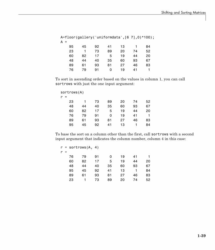
To sort in ascending order based on the values in column 1, you can callsortrows with just the one input argument:
sortrows(A)r =
23 1 73 89 20 74 5248 44 40 35 60 93 6760 82 17 5 19 44 2076 79 91 0 19 41 189 61 93 81 27 46 8395 45 92 41 13 1 84
To base the sort on a column other than the first, call sortrows with a secondinput argument that indicates the column number, column 4 in this case:
r = sortrows(A, 4)r =
76 79 91 0 19 41 160 82 17 5 19 44 2048 44 40 35 60 93 6795 45 92 41 13 1 8489 61 93 81 27 46 8323 1 73 89 20 74 52
1-39
1 Matrices and Arrays
Operating on Diagonal Matrices
In this section...
“Diagonal Matrix Functions” on page 1-40
“Constructing a Matrix from a Diagonal Vector” on page 1-40
“Returning a Triangular Portion of a Matrix” on page 1-41
“Concatenating Matrices Diagonally” on page 1-41
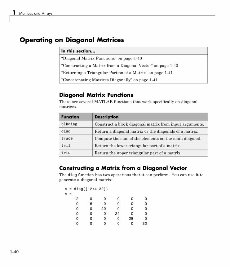
Diagonal Matrix FunctionsThere are several MATLAB functions that work specifically on diagonalmatrices.
Function Description
blkdiag Construct a block diagonal matrix from input arguments.
diag Return a diagonal matrix or the diagonals of a matrix.
trace Compute the sum of the elements on the main diagonal.
tril Return the lower triangular part of a matrix.
triu Return the upper triangular part of a matrix.
Constructing a Matrix from a Diagonal VectorThe diag function has two operations that it can perform. You can use it togenerate a diagonal matrix:
A = diag([12:4:32])A =
12 0 0 0 0 00 16 0 0 0 00 0 20 0 0 00 0 0 24 0 00 0 0 0 28 00 0 0 0 0 32
1-40
Operating on Diagonal Matrices
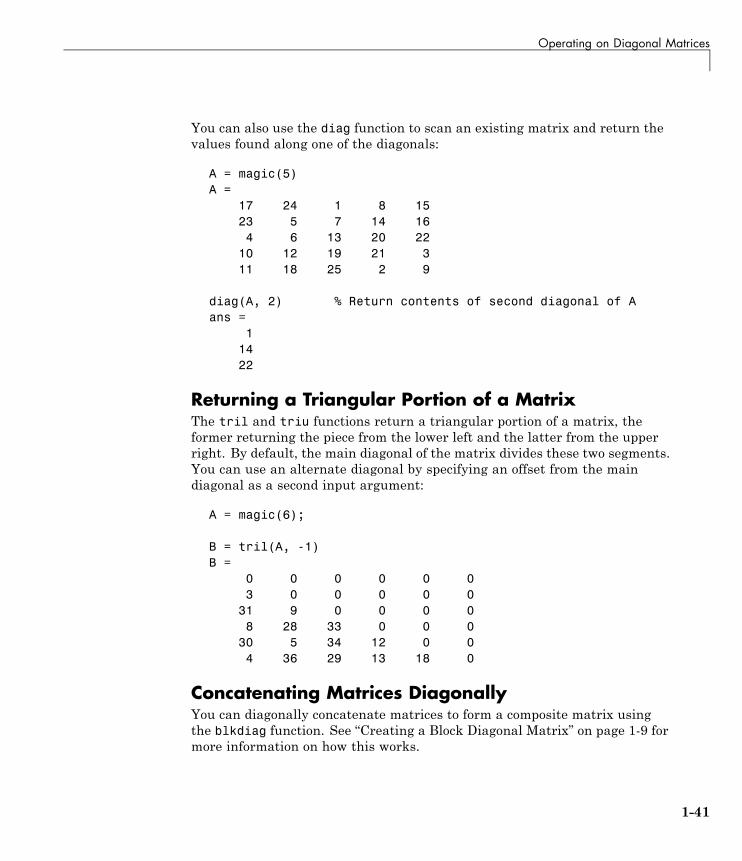
You can also use the diag function to scan an existing matrix and return thevalues found along one of the diagonals:
A = magic(5)A =
17 24 1 8 1523 5 7 14 164 6 13 20 22
10 12 19 21 311 18 25 2 9
diag(A, 2) % Return contents of second diagonal of Aans =
11422
Returning a Triangular Portion of a MatrixThe tril and triu functions return a triangular portion of a matrix, theformer returning the piece from the lower left and the latter from the upperright. By default, the main diagonal of the matrix divides these two segments.You can use an alternate diagonal by specifying an offset from the maindiagonal as a second input argument:
A = magic(6);
B = tril(A, -1)B =
0 0 0 0 0 03 0 0 0 0 0
31 9 0 0 0 08 28 33 0 0 0
30 5 34 12 0 04 36 29 13 18 0
Concatenating Matrices DiagonallyYou can diagonally concatenate matrices to form a composite matrix usingthe blkdiag function. See “Creating a Block Diagonal Matrix” on page 1-9 formore information on how this works.
1-41
1 Matrices and Arrays
Empty Matrices, Scalars, and Vectors
In this section...
“Overview” on page 1-42
“The Empty Matrix” on page 1-43
“Scalars” on page 1-45
“Vectors” on page 1-46
OverviewAlthough matrices are two dimensional, they do not always appear to have arectangular shape. A 1-by-8 matrix, for example, has two dimensions yet islinear. These matrices are described in the following sections:
• “The Empty Matrix” on page 1-43
An empty matrix has one of more dimensions that are equal to zero. Atwo-dimensional matrix with both dimensions equal to zero appears inthe MATLAB application as []. The expression A = [] assigns a 0-by-0empty matrix to A.
• “Scalars” on page 1-45
A scalar is 1-by-1 and appears in MATLAB as a single real or complexnumber (e.g., 7, 583.62, -3.51, 5.46097e-14, 83+4i).
• “Vectors” on page 1-46
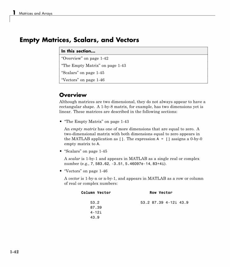
A vector is 1-by-n or n-by-1, and appears in MATLAB as a row or columnof real or complex numbers:
Column Vector Row Vector
53.2 53.2 87.39 4-12i 43.987.394-12i43.9
1-42
Empty Matrices, Scalars, and Vectors
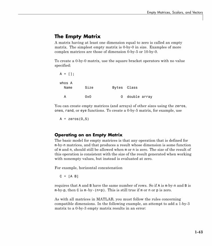
The Empty MatrixA matrix having at least one dimension equal to zero is called an emptymatrix. The simplest empty matrix is 0-by-0 in size. Examples of morecomplex matrices are those of dimension 0-by-5 or 10-by-0.
To create a 0-by-0 matrix, use the square bracket operators with no valuespecified:
A = [];
whos AName Size Bytes Class
A 0x0 0 double array
You can create empty matrices (and arrays) of other sizes using the zeros,ones, rand, or eye functions. To create a 0-by-5 matrix, for example, use
A = zeros(0,5)
Operating on an Empty MatrixThe basic model for empty matrices is that any operation that is defined form-by-n matrices, and that produces a result whose dimension is some functionof m and n, should still be allowed when m or n is zero. The size of the result ofthis operation is consistent with the size of the result generated when workingwith nonempty values, but instead is evaluated at zero.
For example, horizontal concatenation
C = [A B]
requires that A and B have the same number of rows. So if A is m-by-n and B ism-by-p, then C is m-by-(n+p). This is still true if m or n or p is zero.
As with all matrices in MATLAB, you must follow the rules concerningcompatible dimensions. In the following example, an attempt to add a 1-by-3matrix to a 0-by-3 empty matrix results in an error:
1-43
1 Matrices and Arrays
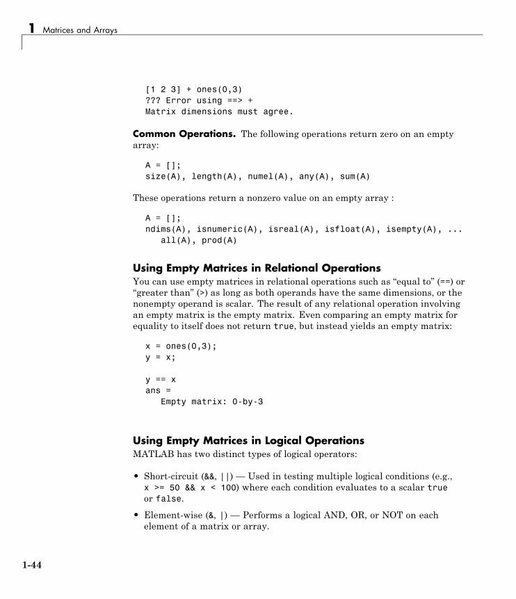
[1 2 3] + ones(0,3)??? Error using ==> +Matrix dimensions must agree.
Common Operations. The following operations return zero on an emptyarray:
A = [];size(A), length(A), numel(A), any(A), sum(A)
These operations return a nonzero value on an empty array :
A = [];ndims(A), isnumeric(A), isreal(A), isfloat(A), isempty(A), ...
all(A), prod(A)
Using Empty Matrices in Relational OperationsYou can use empty matrices in relational operations such as “equal to” (==) or“greater than” (>) as long as both operands have the same dimensions, or thenonempty operand is scalar. The result of any relational operation involvingan empty matrix is the empty matrix. Even comparing an empty matrix forequality to itself does not return true, but instead yields an empty matrix:
x = ones(0,3);y = x;
y == xans =
Empty matrix: 0-by-3
Using Empty Matrices in Logical OperationsMATLAB has two distinct types of logical operators:
• Short-circuit (&&, ||) — Used in testing multiple logical conditions (e.g.,x >= 50 && x < 100) where each condition evaluates to a scalar trueor false.
• Element-wise (&, |) — Performs a logical AND, OR, or NOT on eachelement of a matrix or array.
1-44
Empty Matrices, Scalars, and Vectors
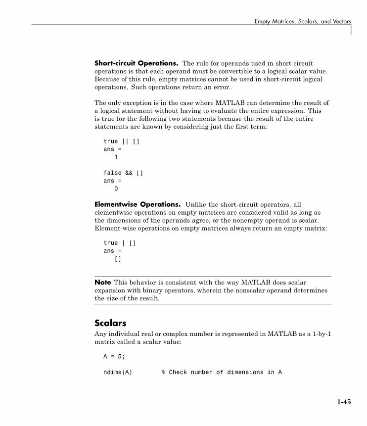
Short-circuit Operations. The rule for operands used in short-circuitoperations is that each operand must be convertible to a logical scalar value.Because of this rule, empty matrices cannot be used in short-circuit logicaloperations. Such operations return an error.
The only exception is in the case where MATLAB can determine the result ofa logical statement without having to evaluate the entire expression. Thisis true for the following two statements because the result of the entirestatements are known by considering just the first term:
true || []ans =
1
false && []ans =
0
Elementwise Operations. Unlike the short-circuit operators, allelementwise operations on empty matrices are considered valid as long asthe dimensions of the operands agree, or the nonempty operand is scalar.Element-wise operations on empty matrices always return an empty matrix:
true | []ans =
[]
Note This behavior is consistent with the way MATLAB does scalarexpansion with binary operators, wherein the nonscalar operand determinesthe size of the result.
ScalarsAny individual real or complex number is represented in MATLAB as a 1-by-1matrix called a scalar value:
A = 5;
ndims(A) % Check number of dimensions in A
1-45
1 Matrices and Arrays
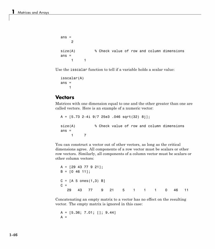
ans =2
size(A) % Check value of row and column dimensionsans =
1 1
Use the isscalar function to tell if a variable holds a scalar value:
isscalar(A)ans =
1
VectorsMatrices with one dimension equal to one and the other greater than one arecalled vectors. Here is an example of a numeric vector:
A = [5.73 2-4i 9/7 25e3 .046 sqrt(32) 8j];
size(A) % Check value of row and column dimensionsans =
1 7
You can construct a vector out of other vectors, as long as the criticaldimensions agree. All components of a row vector must be scalars or otherrow vectors. Similarly, all components of a column vector must be scalars orother column vectors:
A = [29 43 77 9 21];B = [0 46 11];
C = [A 5 ones(1,3) B]C =
29 43 77 9 21 5 1 1 1 0 46 11
Concatenating an empty matrix to a vector has no effect on the resultingvector. The empty matrix is ignored in this case:
A = [5.36; 7.01; []; 9.44]A =
1-46
Empty Matrices, Scalars, and Vectors
5.36007.01009.4400
Use the isvector function to tell if a variable holds a vector:
isvector(A)ans =
1
1-47
1 Matrices and Arrays
Full and Sparse Matrices
In this section...
“Overview” on page 1-48
“Sparse Matrix Functions” on page 1-48
OverviewIt is not uncommon to have matrices with a large number of zero-valuedelements and, because the MATLAB software stores zeros in the same wayit stores any other numeric value, these elements can use memory spaceunnecessarily and can sometimes require extra computing time.
Sparse matrices provide a way to store data that has a large percentage ofzero elements more efficiently. While full matrices internally store everyelement in memory regardless of value, sparse matrices store only the nonzeroelements and their row indices. Using sparse matrices can significantlyreduce the amount of memory required for data storage.
You can create sparse matrices for the double and logical classes. AllMATLAB built-in arithmetic, logical, and indexing operations can be appliedto sparse matrices, or to mixtures of sparse and full matrices. Operationson sparse matrices return sparse matrices and operations on full matricesreturn full matrices.
See the section on Sparse Matrices in the MATLAB Mathematicsdocumentation for more information on working with sparse matrices.
Sparse Matrix FunctionsThis table shows some of the functions most commonly used when workingwith sparse matrices.
Function Description
full Convert a sparse matrix to a full matrix.
issparse Determine if a matrix is sparse.
1-48
Full and Sparse Matrices
Function Description
nnz Return the number of nonzero matrix elements.
nonzeros Return the nonzero elements of a matrix.
nzmax Return the amount of storage allocated for nonzeroelements.
spalloc Allocate space for a sparse matrix.
sparse Create a sparse matrix or convert full to sparse.
speye Create a sparse identity matrix.
sprand Create a sparse uniformly distributed random matrix.
1-49
1 Matrices and Arrays
Multidimensional Arrays
In this section...
“Overview” on page 1-50
“Creating Multidimensional Arrays” on page 1-52
“Accessing Multidimensional Array Properties” on page 1-56
“Indexing Multidimensional Arrays” on page 1-56
“Reshaping Multidimensional Arrays” on page 1-60
“Permuting Array Dimensions” on page 1-62
“Computing with Multidimensional Arrays” on page 1-64
“Organizing Data in Multidimensional Arrays” on page 1-65
“Multidimensional Cell Arrays” on page 1-67
“Multidimensional Structure Arrays” on page 1-68
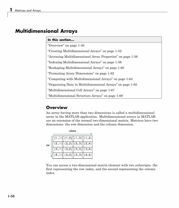
OverviewAn array having more than two dimensions is called a multidimensionalarray in the MATLAB application. Multidimensional arrays in MATLABare an extension of the normal two-dimensional matrix. Matrices have twodimensions: the row dimension and the column dimension.
You can access a two-dimensional matrix element with two subscripts: thefirst representing the row index, and the second representing the columnindex.
1-50
Multidimensional Arrays
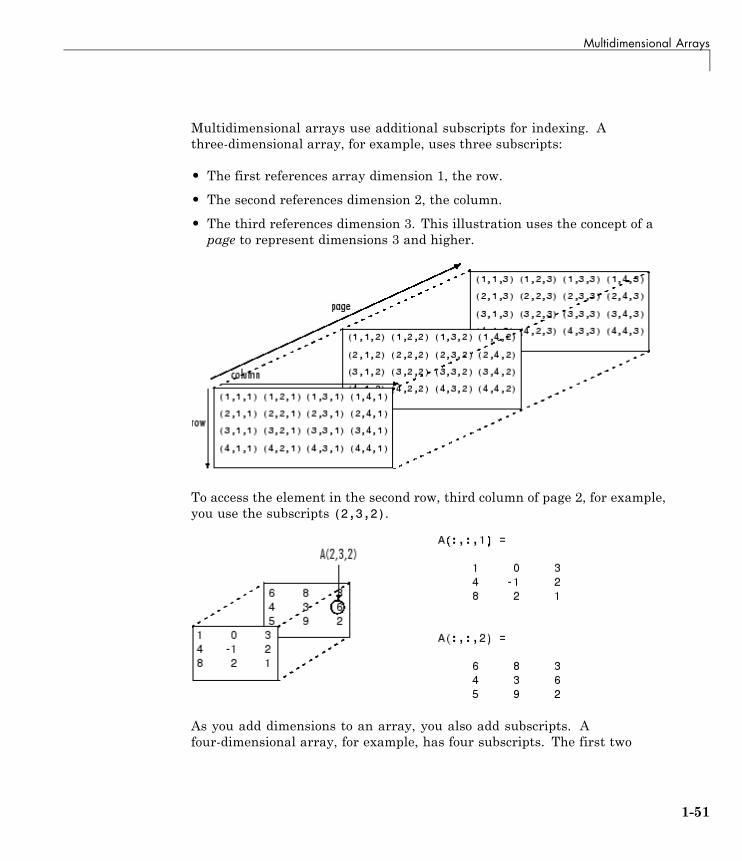
Multidimensional arrays use additional subscripts for indexing. Athree-dimensional array, for example, uses three subscripts:
• The first references array dimension 1, the row.
• The second references dimension 2, the column.
• The third references dimension 3. This illustration uses the concept of apage to represent dimensions 3 and higher.
To access the element in the second row, third column of page 2, for example,you use the subscripts (2,3,2).
As you add dimensions to an array, you also add subscripts. Afour-dimensional array, for example, has four subscripts. The first two
1-51
1 Matrices and Arrays
reference a row-column pair; the second two access the third and fourthdimensions of data.
Most of the operations that you can perform on matrices (i.e., two-dimensionalarrays) can also be done on multidimensional arrays.
Note The general multidimensional array functions reside in the datatypesdirectory.
Creating Multidimensional ArraysYou can use the same techniques to create multidimensional arrays that youuse for two-dimensional matrices. In addition, MATLAB provides a specialconcatenation function that is useful for building multidimensional arrays.
This section discusses
• “Generating Arrays Using Indexing” on page 1-52
• “Extending Multidimensional Arrays” on page 1-53
• “Generating Arrays Using MATLAB Functions” on page 1-54
• “Building Multidimensional Arrays with the cat Function” on page 1-54
Generating Arrays Using IndexingOne way to create a multidimensional array is to create a two-dimensionalarray and extend it. For example, begin with a simple two-dimensionalarray A.
A = [5 7 8; 0 1 9; 4 3 6];
A is a 3-by-3 array, that is, its row dimension is 3 and its column dimensionis 3. To add a third dimension to A,
A(:,:,2) = [1 0 4; 3 5 6; 9 8 7]
MATLAB responds with
A(:,:,1) =
1-52
Multidimensional Arrays
5 7 80 1 94 3 6
A(:,:,2) =1 0 43 5 69 8 7
You can continue to add rows, columns, or pages to the array using similarassignment statements.
Extending Multidimensional ArraysTo extend A in any dimension:
• Increment or add the appropriate subscript and assign the desired values.
• Assign the same number of elements to corresponding array dimensions.For numeric arrays, all rows must have the same number of elements, allpages must have the same number of rows and columns, and so on.
You can take advantage of the MATLAB scalar expansion capabilities,together with the colon operator, to fill an entire dimension with a singlevalue:
A(:,:,3) = 5;
A(:,:,3)ans =
5 5 55 5 55 5 5
To turn A into a 3-by-3-by-3-by-2, four-dimensional array, enter
A(:,:,1,2) = [1 2 3; 4 5 6; 7 8 9];A(:,:,2,2) = [9 8 7; 6 5 4; 3 2 1];A(:,:,3,2) = [1 0 1; 1 1 0; 0 1 1];
1-53
1 Matrices and Arrays
Note that after the first two assignments MATLAB pads A with zeros, asneeded, to maintain the corresponding sizes of dimensions.
Generating Arrays Using MATLAB FunctionsYou can use MATLAB functions such as randn, ones, and zeros to generatemultidimensional arrays in the same way you use them for two-dimensionalarrays. Each argument you supply represents the size of the correspondingdimension in the resulting array. For example, to create a 4-by-3-by-2 arrayof normally distributed random numbers:
B = randn(4,3,2)
To generate an array filled with a single constant value, use the repmatfunction. repmat replicates an array (in this case, a 1-by-1 array) through avector of array dimensions.
B = repmat(5, [3 4 2])
B(:,:,1) =5 5 5 55 5 5 55 5 5 5
B(:,:,2) =5 5 5 55 5 5 55 5 5 5
Note Any dimension of an array can have size zero, making it a form of emptyarray. For example, 10-by-0-by-20 is a valid size for a multidimensional array.
Building Multidimensional Arrays with the cat FunctionThe cat function is a simple way to build multidimensional arrays; itconcatenates a list of arrays along a specified dimension:
B = cat(dim, A1, A2...)
1-54
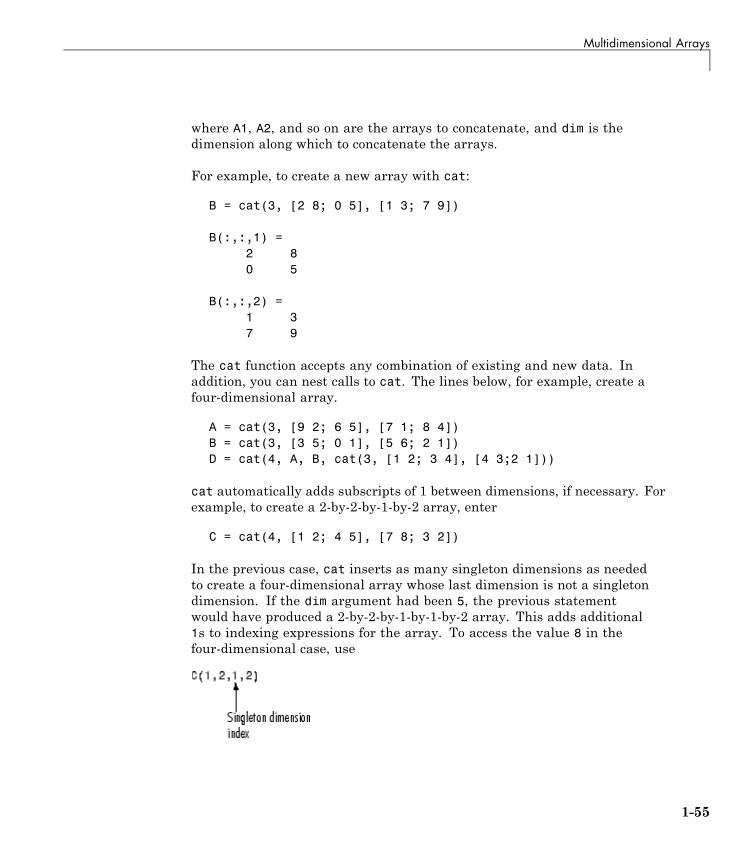
Multidimensional Arrays
where A1, A2, and so on are the arrays to concatenate, and dim is thedimension along which to concatenate the arrays.
For example, to create a new array with cat:
B = cat(3, [2 8; 0 5], [1 3; 7 9])
B(:,:,1) =2 80 5
B(:,:,2) =1 37 9
The cat function accepts any combination of existing and new data. Inaddition, you can nest calls to cat. The lines below, for example, create afour-dimensional array.
A = cat(3, [9 2; 6 5], [7 1; 8 4])B = cat(3, [3 5; 0 1], [5 6; 2 1])D = cat(4, A, B, cat(3, [1 2; 3 4], [4 3;2 1]))
cat automatically adds subscripts of 1 between dimensions, if necessary. Forexample, to create a 2-by-2-by-1-by-2 array, enter
C = cat(4, [1 2; 4 5], [7 8; 3 2])
In the previous case, cat inserts as many singleton dimensions as neededto create a four-dimensional array whose last dimension is not a singletondimension. If the dim argument had been 5, the previous statementwould have produced a 2-by-2-by-1-by-1-by-2 array. This adds additional1s to indexing expressions for the array. To access the value 8 in thefour-dimensional case, use
1-55
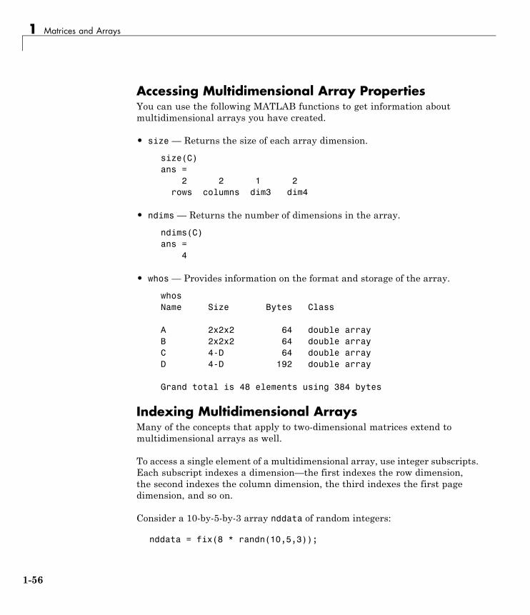
1 Matrices and Arrays
Accessing Multidimensional Array PropertiesYou can use the following MATLAB functions to get information aboutmultidimensional arrays you have created.
• size — Returns the size of each array dimension.
size(C)ans =
2 2 1 2rows columns dim3 dim4
• ndims— Returns the number of dimensions in the array.
ndims(C)ans =
4
• whos— Provides information on the format and storage of the array.
whosName Size Bytes Class
A 2x2x2 64 double arrayB 2x2x2 64 double arrayC 4-D 64 double arrayD 4-D 192 double array
Grand total is 48 elements using 384 bytes
Indexing Multidimensional ArraysMany of the concepts that apply to two-dimensional matrices extend tomultidimensional arrays as well.
To access a single element of a multidimensional array, use integer subscripts.Each subscript indexes a dimension—the first indexes the row dimension,the second indexes the column dimension, the third indexes the first pagedimension, and so on.
Consider a 10-by-5-by-3 array nddata of random integers:
nddata = fix(8 * randn(10,5,3));
1-56
Multidimensional Arrays
To access element (3,2) on page 2 of nddata, for example, use nddata(3,2,2).
You can use vectors as array subscripts. In this case, each vector elementmust be a valid subscript, that is, within the bounds defined by thedimensions of the array. To access elements (2,1), (2,3), and (2,4) onpage 3 of nddata, use
nddata(2,[1 3 4],3);
The Colon and Multidimensional Array IndexingThe MATLAB colon indexing extends to multidimensional arrays. Forexample, to access the entire third column on page 2 of nddata, usenddata(:,3,2).
The colon operator is also useful for accessing other subsets of data. Forexample, nddata(2:3,2:3,1) results in a 2-by-2 array, a subset of the dataon page 1 of nddata. This matrix consists of the data in rows 2 and 3, columns2 and 3, on the first page of the array.
The colon operator can appear as an array subscript on both sides of anassignment statement. For example, to create a 4-by-4 array of zeros:
C = zeros(4, 4)
Now assign a 2-by-2 subset of array nddata to the four elements in the centerof C.
C(2:3,2:3) = nddata(2:3,1:2,2)
Linear Indexing with Multidimensional ArraysMATLAB linear indexing also extends to multidimensional arrays. In thiscase, MATLAB operates on a page-by-page basis to create the storage column,again appending elements columnwise. See “Linear Indexing” on page 1-13for an introduction to this topic.
1-57
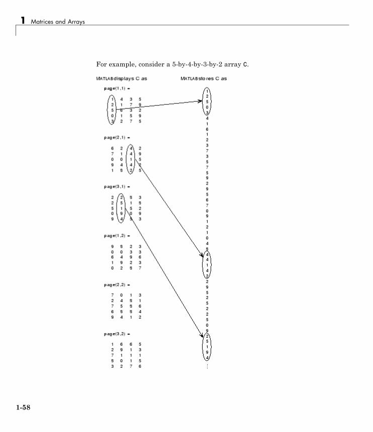
1 Matrices and Arrays
For example, consider a 5-by-4-by-3-by-2 array C.
1-58
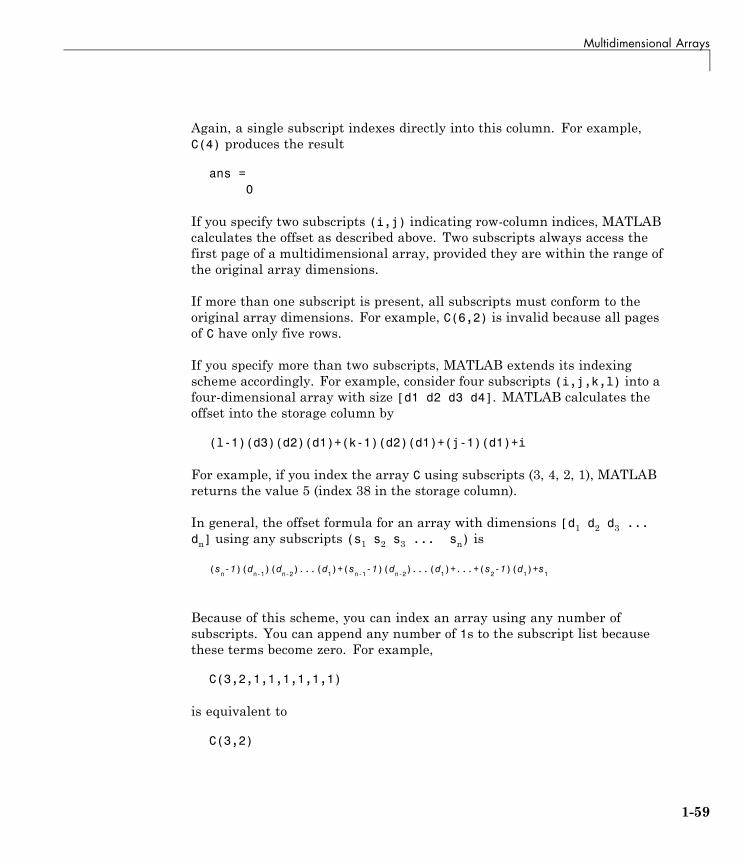
Multidimensional Arrays
Again, a single subscript indexes directly into this column. For example,C(4) produces the result
ans =0
If you specify two subscripts (i,j) indicating row-column indices, MATLABcalculates the offset as described above. Two subscripts always access thefirst page of a multidimensional array, provided they are within the range ofthe original array dimensions.
If more than one subscript is present, all subscripts must conform to theoriginal array dimensions. For example, C(6,2) is invalid because all pagesof C have only five rows.
If you specify more than two subscripts, MATLAB extends its indexingscheme accordingly. For example, consider four subscripts (i,j,k,l) into afour-dimensional array with size [d1 d2 d3 d4]. MATLAB calculates theoffset into the storage column by
(l-1)(d3)(d2)(d1)+(k-1)(d2)(d1)+(j-1)(d1)+i
For example, if you index the array C using subscripts (3, 4, 2, 1), MATLABreturns the value 5 (index 38 in the storage column).
In general, the offset formula for an array with dimensions [d1 d2 d3 ...dn] using any subscripts (s1 s2 s3 ... sn) is
(sn-1)(d
n-1)(d
n-2)...(d
1)+(s
n-1-1)(d
n-2)...(d
1)+...+(s
2-1)(d
1)+s
1
Because of this scheme, you can index an array using any number ofsubscripts. You can append any number of 1s to the subscript list becausethese terms become zero. For example,
C(3,2,1,1,1,1,1,1)
is equivalent to
C(3,2)
1-59
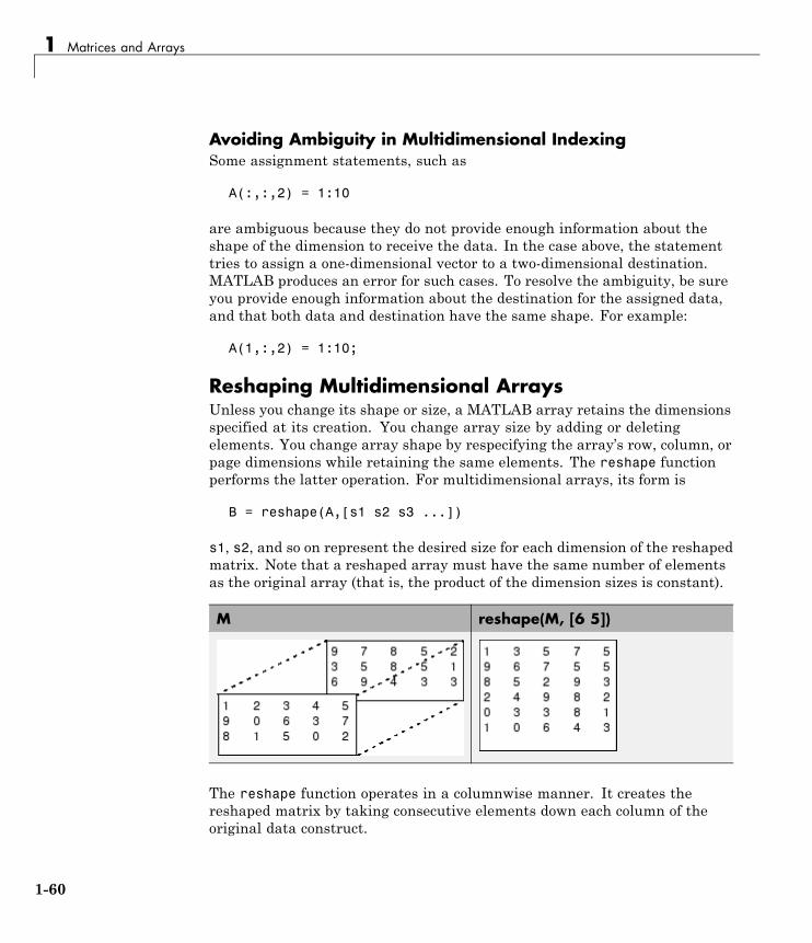
1 Matrices and Arrays
Avoiding Ambiguity in Multidimensional IndexingSome assignment statements, such as
A(:,:,2) = 1:10
are ambiguous because they do not provide enough information about theshape of the dimension to receive the data. In the case above, the statementtries to assign a one-dimensional vector to a two-dimensional destination.MATLAB produces an error for such cases. To resolve the ambiguity, be sureyou provide enough information about the destination for the assigned data,and that both data and destination have the same shape. For example:
A(1,:,2) = 1:10;
Reshaping Multidimensional ArraysUnless you change its shape or size, a MATLAB array retains the dimensionsspecified at its creation. You change array size by adding or deletingelements. You change array shape by respecifying the array’s row, column, orpage dimensions while retaining the same elements. The reshape functionperforms the latter operation. For multidimensional arrays, its form is
B = reshape(A,[s1 s2 s3 ...])
s1, s2, and so on represent the desired size for each dimension of the reshapedmatrix. Note that a reshaped array must have the same number of elementsas the original array (that is, the product of the dimension sizes is constant).
M reshape(M, [6 5])
The reshape function operates in a columnwise manner. It creates thereshaped matrix by taking consecutive elements down each column of theoriginal data construct.
1-60
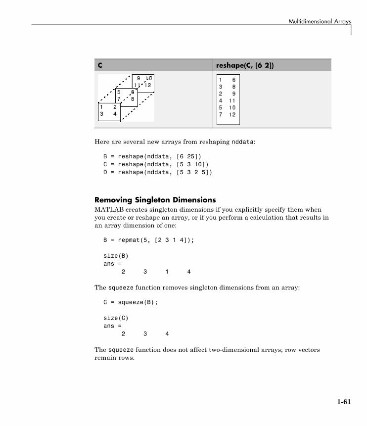
Multidimensional Arrays
C reshape(C, [6 2])
Here are several new arrays from reshaping nddata:
B = reshape(nddata, [6 25])C = reshape(nddata, [5 3 10])D = reshape(nddata, [5 3 2 5])
Removing Singleton DimensionsMATLAB creates singleton dimensions if you explicitly specify them whenyou create or reshape an array, or if you perform a calculation that results inan array dimension of one:
B = repmat(5, [2 3 1 4]);
size(B)ans =
2 3 1 4
The squeeze function removes singleton dimensions from an array:
C = squeeze(B);
size(C)ans =
2 3 4
The squeeze function does not affect two-dimensional arrays; row vectorsremain rows.
1-61
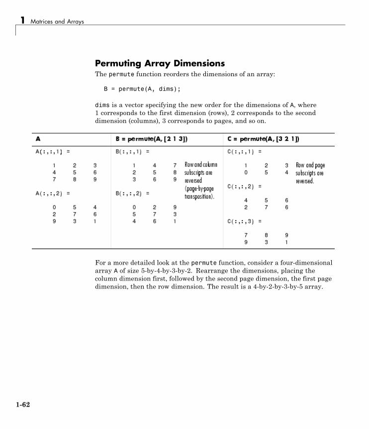
1 Matrices and Arrays
Permuting Array DimensionsThe permute function reorders the dimensions of an array:
B = permute(A, dims);
dims is a vector specifying the new order for the dimensions of A, where1 corresponds to the first dimension (rows), 2 corresponds to the seconddimension (columns), 3 corresponds to pages, and so on.
For a more detailed look at the permute function, consider a four-dimensionalarray A of size 5-by-4-by-3-by-2. Rearrange the dimensions, placing thecolumn dimension first, followed by the second page dimension, the first pagedimension, then the row dimension. The result is a 4-by-2-by-3-by-5 array.
1-62
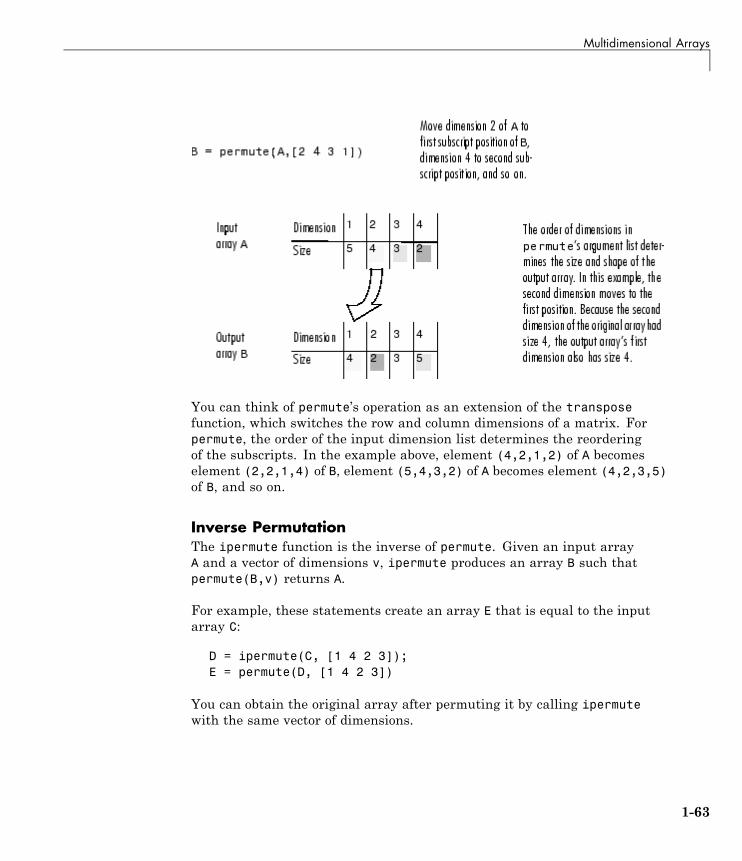
Multidimensional Arrays
You can think of permute’s operation as an extension of the transposefunction, which switches the row and column dimensions of a matrix. Forpermute, the order of the input dimension list determines the reorderingof the subscripts. In the example above, element (4,2,1,2) of A becomeselement (2,2,1,4) of B, element (5,4,3,2) of A becomes element (4,2,3,5)of B, and so on.
Inverse PermutationThe ipermute function is the inverse of permute. Given an input arrayA and a vector of dimensions v, ipermute produces an array B such thatpermute(B,v) returns A.
For example, these statements create an array E that is equal to the inputarray C:
D = ipermute(C, [1 4 2 3]);E = permute(D, [1 4 2 3])
You can obtain the original array after permuting it by calling ipermutewith the same vector of dimensions.
1-63
1 Matrices and Arrays
Computing with Multidimensional ArraysMany of the MATLAB computational and mathematical functions acceptmultidimensional arrays as arguments. These functions operate on specificdimensions of multidimensional arrays; that is, they operate on individualelements, on vectors, or on matrices.
Operating on VectorsFunctions that operate on vectors, like sum, mean, and so on, by defaulttypically work on the first nonsingleton dimension of a multidimensionalarray. Most of these functions optionally let you specify a particulardimension on which to operate. There are exceptions, however. For example,the cross function, which finds the cross product of two vectors, works on thefirst nonsingleton dimension having length 3.
Note In many cases, these functions have other restrictions on the inputarguments — for example, some functions that accept multiple arrays requirethat the arrays be the same size. Refer to the online help for details onfunction arguments.
Operating Element-by-ElementMATLAB functions that operate element-by-element on two-dimensionalarrays, like the trigonometric and exponential functions in the elfundirectory, work in exactly the same way for multidimensional cases. Forexample, the sin function returns an array the same size as the function’sinput argument. Each element of the output array is the sine of thecorresponding element of the input array.
Similarly, the arithmetic, logical, and relational operators all work withcorresponding elements of multidimensional arrays that are the same size inevery dimension. If one operand is a scalar and one an array, the operatorapplies the scalar to each element of the array.
Operating on Planes and MatricesFunctions that operate on planes or matrices, such as the linear algebra andmatrix functions in the matfun directory, do not accept multidimensional
1-64

Multidimensional Arrays
arrays as arguments. That is, you cannot use the functions in the matfundirectory, or the array operators *, ^, \, or /, with multidimensionalarguments. Supplying multidimensional arguments or operands in thesecases results in an error.
You can use indexing to apply a matrix function or operator to matrices withina multidimensional array. For example, create a three-dimensional array A:
A = cat(3, [1 2 3; 9 8 7; 4 6 5], [0 3 2; 8 8 4; 5 3 5], ...[6 4 7; 6 8 5; 5 4 3]);
Applying the eig function to the entire multidimensional array results inan error:
eig(A)??? Error using ==> eigInput arguments must be 2-D.
You can, however, apply eig to planes within the array. For example, usecolon notation to index just one page (in this case, the second) of the array:
eig(A(:,:,2))ans =
12.9129-2.62602.7131
Note In the first case, subscripts are not colons; you must use squeeze toavoid an error. For example, eig(A(2,:,:)) results in an error becausethe size of the input is [1 3 3]. The expression eig(squeeze(A(2,:,:))),however, passes a valid two-dimensional matrix to eig.
Organizing Data in Multidimensional ArraysYou can use multidimensional arrays to represent data in two ways:
• As planes or pages of two-dimensional data. You can then treat these pagesas matrices.
1-65
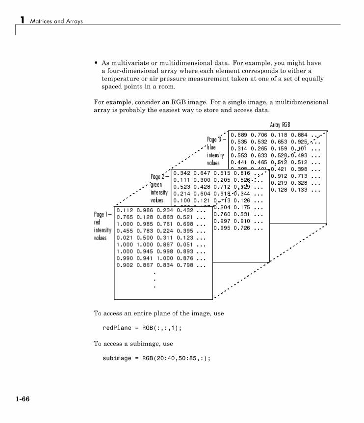
1 Matrices and Arrays
• As multivariate or multidimensional data. For example, you might havea four-dimensional array where each element corresponds to either atemperature or air pressure measurement taken at one of a set of equallyspaced points in a room.
For example, consider an RGB image. For a single image, a multidimensionalarray is probably the easiest way to store and access data.
To access an entire plane of the image, use
redPlane = RGB(:,:,1);
To access a subimage, use
subimage = RGB(20:40,50:85,:);
1-66
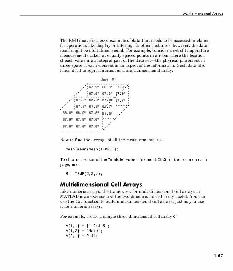
Multidimensional Arrays
The RGB image is a good example of data that needs to be accessed in planesfor operations like display or filtering. In other instances, however, the dataitself might be multidimensional. For example, consider a set of temperaturemeasurements taken at equally spaced points in a room. Here the locationof each value is an integral part of the data set—the physical placement inthree-space of each element is an aspect of the information. Such data alsolends itself to representation as a multidimensional array.
Now to find the average of all the measurements, use
mean(mean(mean(TEMP)));
To obtain a vector of the “middle” values (element (2,2)) in the room on eachpage, use
B = TEMP(2,2,:);
Multidimensional Cell ArraysLike numeric arrays, the framework for multidimensional cell arrays inMATLAB is an extension of the two-dimensional cell array model. You canuse the cat function to build multidimensional cell arrays, just as you useit for numeric arrays.
For example, create a simple three-dimensional cell array C:
A{1,1} = [1 2;4 5];A{1,2} = 'Name';A{2,1} = 2-4i;
1-67
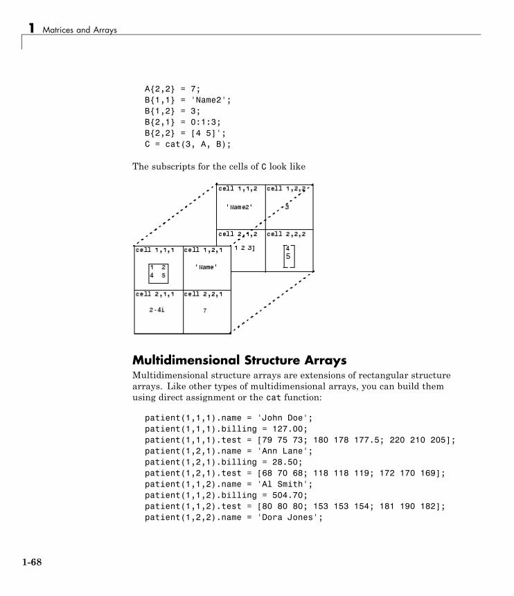
1 Matrices and Arrays
A{2,2} = 7;B{1,1} = 'Name2';B{1,2} = 3;B{2,1} = 0:1:3;B{2,2} = [4 5]';C = cat(3, A, B);
The subscripts for the cells of C look like
Multidimensional Structure ArraysMultidimensional structure arrays are extensions of rectangular structurearrays. Like other types of multidimensional arrays, you can build themusing direct assignment or the cat function:
patient(1,1,1).name = 'John Doe';patient(1,1,1).billing = 127.00;patient(1,1,1).test = [79 75 73; 180 178 177.5; 220 210 205];patient(1,2,1).name = 'Ann Lane';patient(1,2,1).billing = 28.50;patient(1,2,1).test = [68 70 68; 118 118 119; 172 170 169];patient(1,1,2).name = 'Al Smith';patient(1,1,2).billing = 504.70;patient(1,1,2).test = [80 80 80; 153 153 154; 181 190 182];patient(1,2,2).name = 'Dora Jones';
1-68
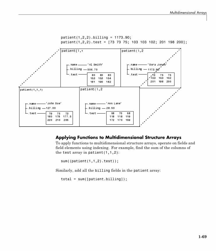
Multidimensional Arrays
patient(1,2,2).billing = 1173.90;patient(1,2,2).test = [73 73 75; 103 103 102; 201 198 200];
Applying Functions to Multidimensional Structure ArraysTo apply functions to multidimensional structure arrays, operate on fields andfield elements using indexing. For example, find the sum of the columns ofthe test array in patient(1,1,2):
sum((patient(1,1,2).test));
Similarly, add all the billing fields in the patient array:
total = sum([patient.billing]);
1-69
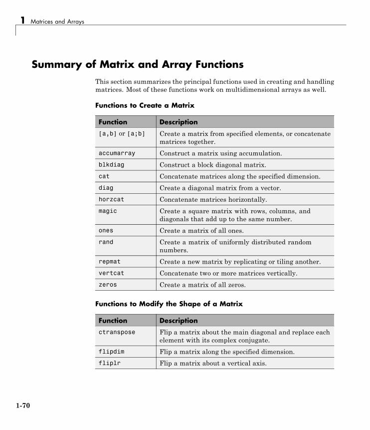
1 Matrices and Arrays
Summary of Matrix and Array FunctionsThis section summarizes the principal functions used in creating and handlingmatrices. Most of these functions work on multidimensional arrays as well.
Functions to Create a Matrix
Function Description
[a,b] or [a;b] Create a matrix from specified elements, or concatenatematrices together.
accumarray Construct a matrix using accumulation.
blkdiag Construct a block diagonal matrix.
cat Concatenate matrices along the specified dimension.
diag Create a diagonal matrix from a vector.
horzcat Concatenate matrices horizontally.
magic Create a square matrix with rows, columns, anddiagonals that add up to the same number.
ones Create a matrix of all ones.
rand Create a matrix of uniformly distributed randomnumbers.
repmat Create a new matrix by replicating or tiling another.
vertcat Concatenate two or more matrices vertically.
zeros Create a matrix of all zeros.
Functions to Modify the Shape of a Matrix
Function Description
ctranspose Flip a matrix about the main diagonal and replace eachelement with its complex conjugate.
flipdim Flip a matrix along the specified dimension.
fliplr Flip a matrix about a vertical axis.
1-70
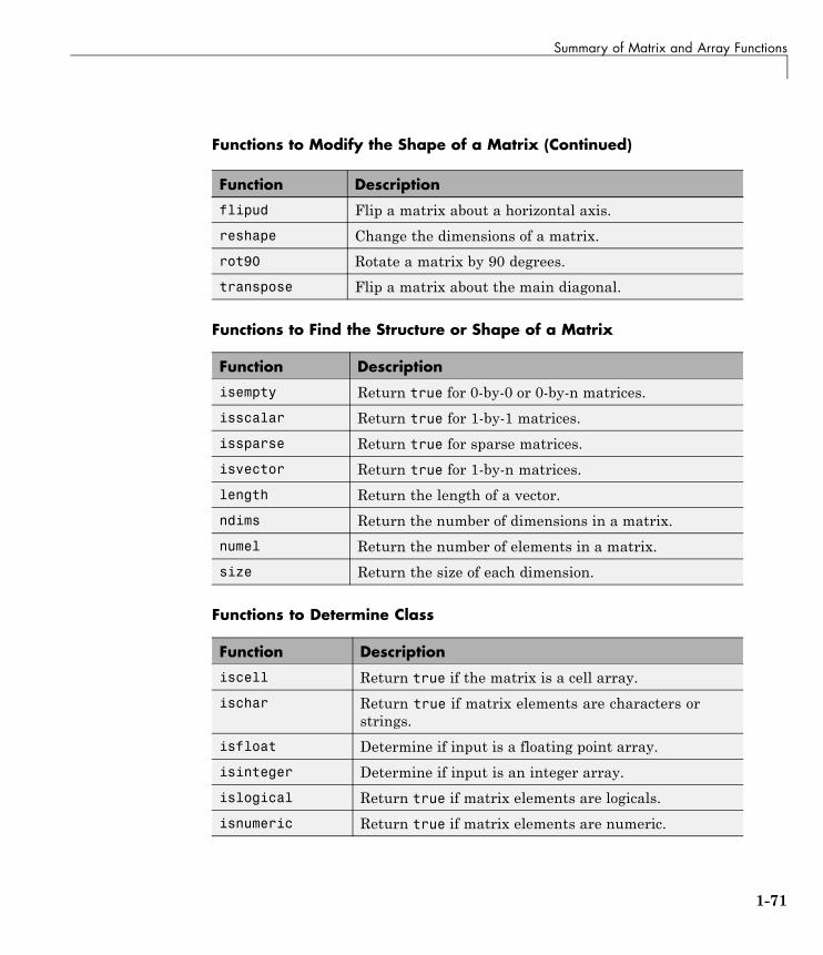
Summary of Matrix and Array Functions
Functions to Modify the Shape of a Matrix (Continued)
Function Description
flipud Flip a matrix about a horizontal axis.
reshape Change the dimensions of a matrix.
rot90 Rotate a matrix by 90 degrees.
transpose Flip a matrix about the main diagonal.
Functions to Find the Structure or Shape of a Matrix
Function Description
isempty Return true for 0-by-0 or 0-by-n matrices.
isscalar Return true for 1-by-1 matrices.
issparse Return true for sparse matrices.
isvector Return true for 1-by-n matrices.
length Return the length of a vector.
ndims Return the number of dimensions in a matrix.
numel Return the number of elements in a matrix.
size Return the size of each dimension.
Functions to Determine Class
Function Description
iscell Return true if the matrix is a cell array.
ischar Return true if matrix elements are characters orstrings.
isfloat Determine if input is a floating point array.
isinteger Determine if input is an integer array.
islogical Return true if matrix elements are logicals.
isnumeric Return true if matrix elements are numeric.
1-71
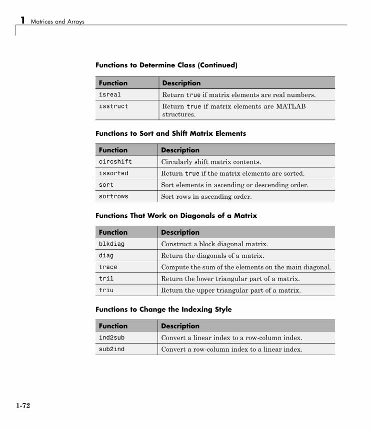
1 Matrices and Arrays
Functions to Determine Class (Continued)
Function Description
isreal Return true if matrix elements are real numbers.
isstruct Return true if matrix elements are MATLABstructures.
Functions to Sort and Shift Matrix Elements
Function Description
circshift Circularly shift matrix contents.
issorted Return true if the matrix elements are sorted.
sort Sort elements in ascending or descending order.
sortrows Sort rows in ascending order.
Functions That Work on Diagonals of a Matrix
Function Description
blkdiag Construct a block diagonal matrix.
diag Return the diagonals of a matrix.
trace Compute the sum of the elements on the main diagonal.
tril Return the lower triangular part of a matrix.
triu Return the upper triangular part of a matrix.
Functions to Change the Indexing Style
Function Description
ind2sub Convert a linear index to a row-column index.
sub2ind Convert a row-column index to a linear index.
1-72
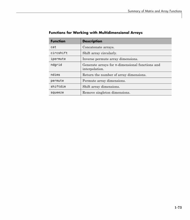
Summary of Matrix and Array Functions
Functions for Working with Multidimensional Arrays
Function Description
cat Concatenate arrays.
circshift Shift array circularly.
ipermute Inverse permute array dimensions.
ndgrid Generate arrays for n-dimensional functions andinterpolation.
ndims Return the number of array dimensions.
permute Permute array dimensions.
shiftdim Shift array dimensions.
squeeze Remove singleton dimensions.
1-73

1 Matrices and Arrays
1-74
2
Linear Algebra
• “MATLAB Linear Algebra Functions” on page 2-2
• “Matrices in the MATLAB Environment” on page 2-5
• “Systems of Linear Equations” on page 2-15
• “Inverses and Determinants” on page 2-26
• “Factorizations” on page 2-31
• “Powers and Exponentials” on page 2-40
• “Eigenvalues” on page 2-44
• “Singular Values” on page 2-48
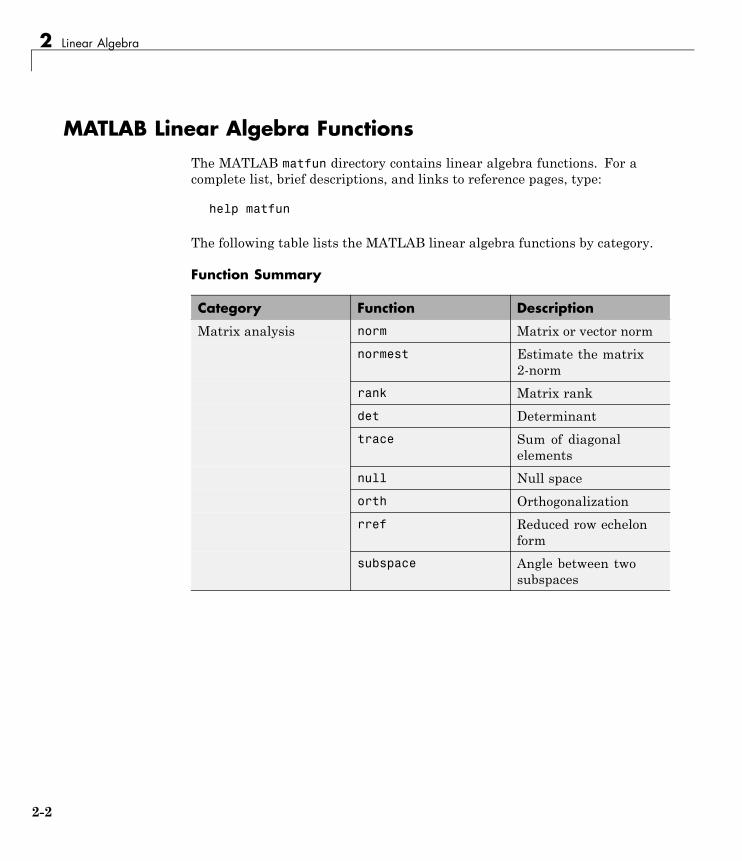
2 Linear Algebra
MATLAB Linear Algebra FunctionsThe MATLAB matfun directory contains linear algebra functions. For acomplete list, brief descriptions, and links to reference pages, type:
help matfun
The following table lists the MATLAB linear algebra functions by category.
Function Summary
Category Function Description
norm Matrix or vector norm
normest Estimate the matrix2-norm
rank Matrix rank
det Determinant
trace Sum of diagonalelements
null Null space
orth Orthogonalization
rref Reduced row echelonform
Matrix analysis
subspace Angle between twosubspaces
2-2
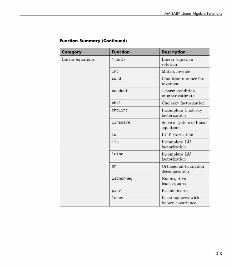
MATLAB® Linear Algebra Functions
Function Summary (Continued)
Category Function Description
\ and / Linear equationsolution
inv Matrix inverse
cond Condition number forinversion
condest 1-norm conditionnumber estimate
chol Cholesky factorization
cholinc Incomplete Choleskyfactorization
linsolve Solve a system of linearequations
lu LU factorization
ilu Incomplete LUfactorization
luinc Incomplete LUfactorization
qr Orthogonal-triangulardecomposition
lsqnonneg Nonnegativeleast-squares
pinv Pseudoinverse
Linear equations
lscov Least squares withknown covariance
2-3
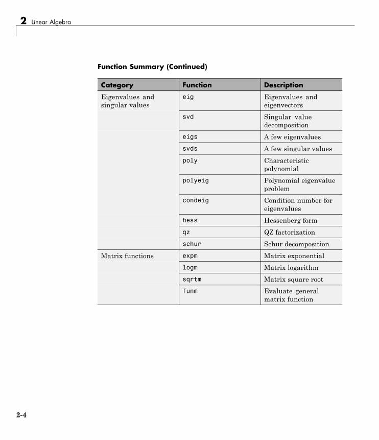
2 Linear Algebra
Function Summary (Continued)
Category Function Description
eig Eigenvalues andeigenvectors
svd Singular valuedecomposition
eigs A few eigenvalues
svds A few singular values
poly Characteristicpolynomial
polyeig Polynomial eigenvalueproblem
condeig Condition number foreigenvalues
hess Hessenberg form
qz QZ factorization
Eigenvalues andsingular values
schur Schur decomposition
expm Matrix exponential
logm Matrix logarithm
sqrtm Matrix square root
Matrix functions
funm Evaluate generalmatrix function
2-4
Matrices in the MATLAB® Environment
Matrices in the MATLAB Environment
In this section...
“Creating Matrices” on page 2-5
“Adding and Subtracting Matrices” on page 2-7
“Vector Products and Transpose” on page 2-7
“Multiplying Matrices” on page 2-9
“Identity Matrix” on page 2-11
“Kronecker Tensor Product” on page 2-12
“Vector and Matrix Norms” on page 2-13
“Using Multithreaded Computation with Linear Algebra Functions” onpage 2-14
Creating MatricesThe MATLAB environment uses the term matrix to indicate a variablecontaining real or complex numbers arranged in a two-dimensional grid.An array is, more generally, a vector, matrix, or higher-dimensional gridof numbers. All arrays in MATLAB are rectangular, in the sense that thecomponent vectors along any dimension are all the same length.
Symbolic Math Toolbox™ software extends the capabilities of MATLABsoftware to matrices of mathematical expressions.
MATLAB has dozens of functions that create different kinds of matrices.There are two functions you can use to create a pair of 3-by-3 examplematrices for use throughout this chapter. The first example is symmetric:
A = pascal(3)
A =1 1 11 2 31 3 6
The second example is not symmetric:
2-5

2 Linear Algebra
B = magic(3)
B =8 1 63 5 74 9 2
Another example is a 3-by-2 rectangular matrix of random integers:
C = fix(10*rand(3,2))
C =9 42 86 7
A column vector is an m-by-1 matrix, a row vector is a 1-by-n matrix, and ascalar is a 1-by-1 matrix. The statements
u = [3; 1; 4]
v = [2 0 -1]
s = 7
produce a column vector, a row vector, and a scalar:
u =314
v =2 0 -1
s =7
For more information about creating and working with matrices, see inMATLAB Programming Fundamentals.
2-6

Matrices in the MATLAB® Environment
Adding and Subtracting MatricesAddition and subtraction of matrices is defined just as it is for arrays, elementby element. Adding A to B and then subtracting A from the result recovers B:
A = pascal(3);B = magic(3);X = A + B
X =9 2 74 7 105 12 8
Y = X - A
Y =8 1 63 5 74 9 2
Addition and subtraction require both matrices to have the same dimension, orone of them be a scalar. If the dimensions are incompatible, an error results:
C = fix(10*rand(3,2))X = A + CError using ==> +Matrix dimensions must agree.
w = v + s
w =9 7 6
Vector Products and TransposeA row vector and a column vector of the same length can be multiplied ineither order. The result is either a scalar, the inner product, or a matrix,the outer product :
u = [3; 1; 4];v = [2 0 -1];
2-7
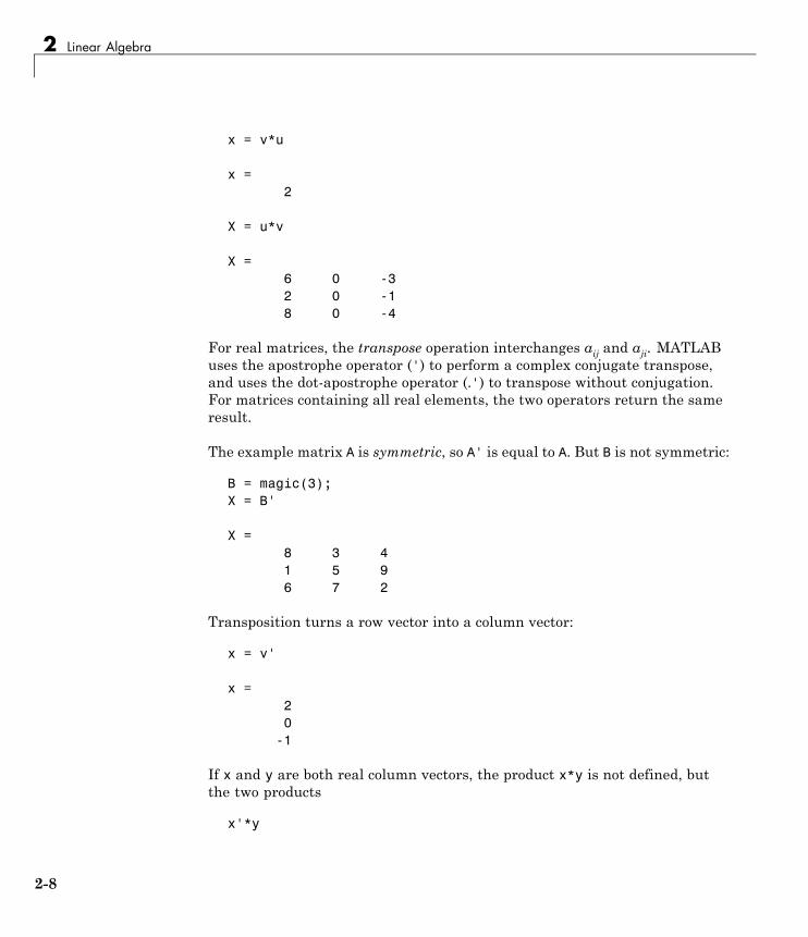
2 Linear Algebra
x = v*u
x =2
X = u*v
X =6 0 -32 0 -18 0 -4
For real matrices, the transpose operation interchanges aij and aji. MATLABuses the apostrophe operator (') to perform a complex conjugate transpose,and uses the dot-apostrophe operator (.') to transpose without conjugation.For matrices containing all real elements, the two operators return the sameresult.
The example matrix A is symmetric, so A' is equal to A. But B is not symmetric:
B = magic(3);X = B'
X =8 3 41 5 96 7 2
Transposition turns a row vector into a column vector:
x = v'
x =20
-1
If x and y are both real column vectors, the product x*y is not defined, butthe two products
x'*y
2-8
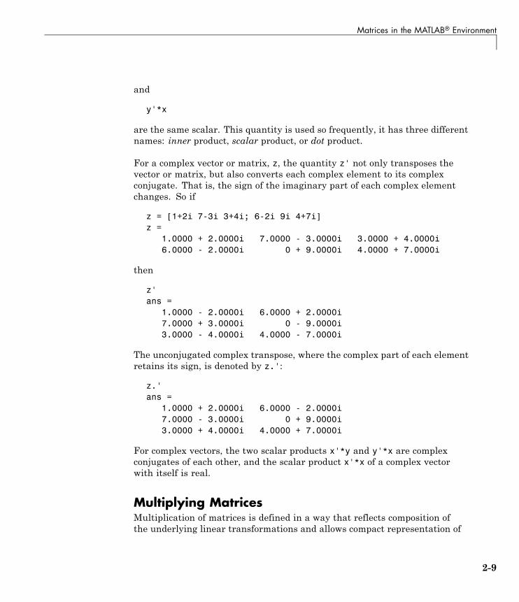
Matrices in the MATLAB® Environment
and
y'*x
are the same scalar. This quantity is used so frequently, it has three differentnames: inner product, scalar product, or dot product.
For a complex vector or matrix, z, the quantity z' not only transposes thevector or matrix, but also converts each complex element to its complexconjugate. That is, the sign of the imaginary part of each complex elementchanges. So if
z = [1+2i 7-3i 3+4i; 6-2i 9i 4+7i]z =
1.0000 + 2.0000i 7.0000 - 3.0000i 3.0000 + 4.0000i6.0000 - 2.0000i 0 + 9.0000i 4.0000 + 7.0000i
then
z'ans =
1.0000 - 2.0000i 6.0000 + 2.0000i7.0000 + 3.0000i 0 - 9.0000i3.0000 - 4.0000i 4.0000 - 7.0000i
The unconjugated complex transpose, where the complex part of each elementretains its sign, is denoted by z.':
z.'ans =
1.0000 + 2.0000i 6.0000 - 2.0000i7.0000 - 3.0000i 0 + 9.0000i3.0000 + 4.0000i 4.0000 + 7.0000i
For complex vectors, the two scalar products x'*y and y'*x are complexconjugates of each other, and the scalar product x'*x of a complex vectorwith itself is real.
Multiplying MatricesMultiplication of matrices is defined in a way that reflects composition ofthe underlying linear transformations and allows compact representation of
2-9
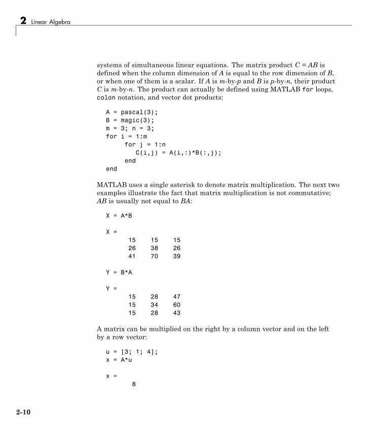
2 Linear Algebra
systems of simultaneous linear equations. The matrix product C = AB isdefined when the column dimension of A is equal to the row dimension of B,or when one of them is a scalar. If A is m-by-p and B is p-by-n, their productC is m-by-n. The product can actually be defined using MATLAB for loops,colon notation, and vector dot products:
A = pascal(3);B = magic(3);m = 3; n = 3;for i = 1:m
for j = 1:nC(i,j) = A(i,:)*B(:,j);
endend
MATLAB uses a single asterisk to denote matrix multiplication. The next twoexamples illustrate the fact that matrix multiplication is not commutative;AB is usually not equal to BA:
X = A*B
X =15 15 1526 38 2641 70 39
Y = B*A
Y =15 28 4715 34 6015 28 43
A matrix can be multiplied on the right by a column vector and on the leftby a row vector:
u = [3; 1; 4];x = A*u
x =8
2-10
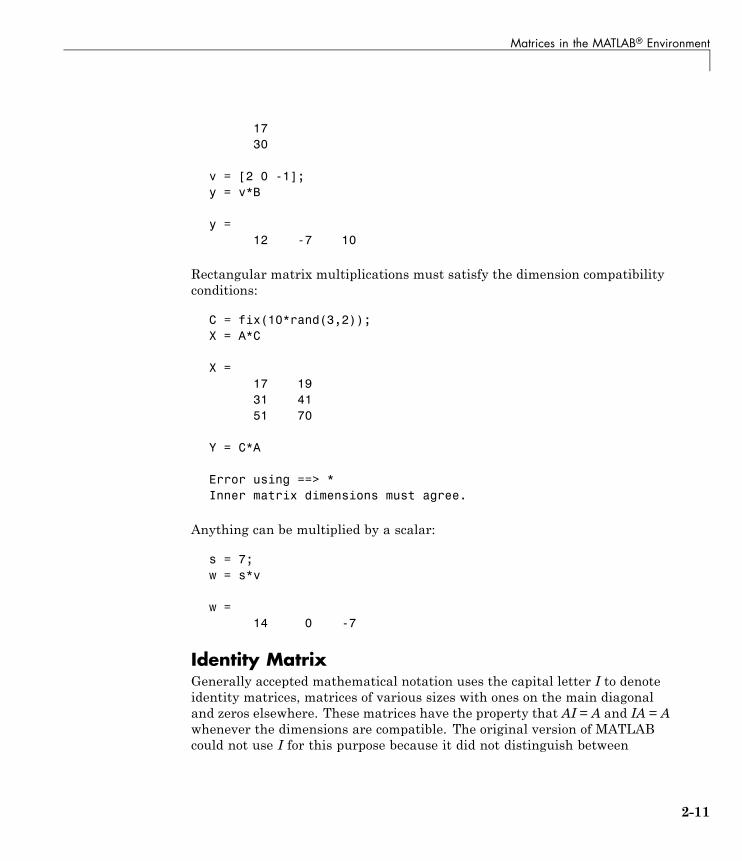
Matrices in the MATLAB® Environment
1730
v = [2 0 -1];y = v*B
y =12 -7 10
Rectangular matrix multiplications must satisfy the dimension compatibilityconditions:
C = fix(10*rand(3,2));X = A*C
X =17 1931 4151 70
Y = C*A
Error using ==> *Inner matrix dimensions must agree.
Anything can be multiplied by a scalar:
s = 7;w = s*v
w =14 0 -7
Identity MatrixGenerally accepted mathematical notation uses the capital letter I to denoteidentity matrices, matrices of various sizes with ones on the main diagonaland zeros elsewhere. These matrices have the property that AI = A and IA = Awhenever the dimensions are compatible. The original version of MATLABcould not use I for this purpose because it did not distinguish between
2-11

2 Linear Algebra
uppercase and lowercase letters and i already served as a subscript and as thecomplex unit. So an English language pun was introduced. The function
eye(m,n)
returns an m-by-n rectangular identity matrix and eye(n) returns an n-by-nsquare identity matrix.
Kronecker Tensor ProductThe Kronecker product, kron(X,Y), of two matrices is the larger matrixformed from all possible products of the elements of X with those of Y. If Xis m-by-n and Y is p-by-q, then kron(X,Y) is mp-by-nq. The elements arearranged in the following order:
[X(1,1)*Y X(1,2)*Y . . . X(1,n)*Y. . .
X(m,1)*Y X(m,2)*Y . . . X(m,n)*Y]
The Kronecker product is often used with matrices of zeros and ones to buildup repeated copies of small matrices. For example, if X is the 2-by-2 matrix
X =1 23 4
and I = eye(2,2) is the 2-by-2 identity matrix, then the two matrices
kron(X,I)
and
kron(I,X)
are
1 0 2 00 1 0 23 0 4 00 3 0 4
and
2-12
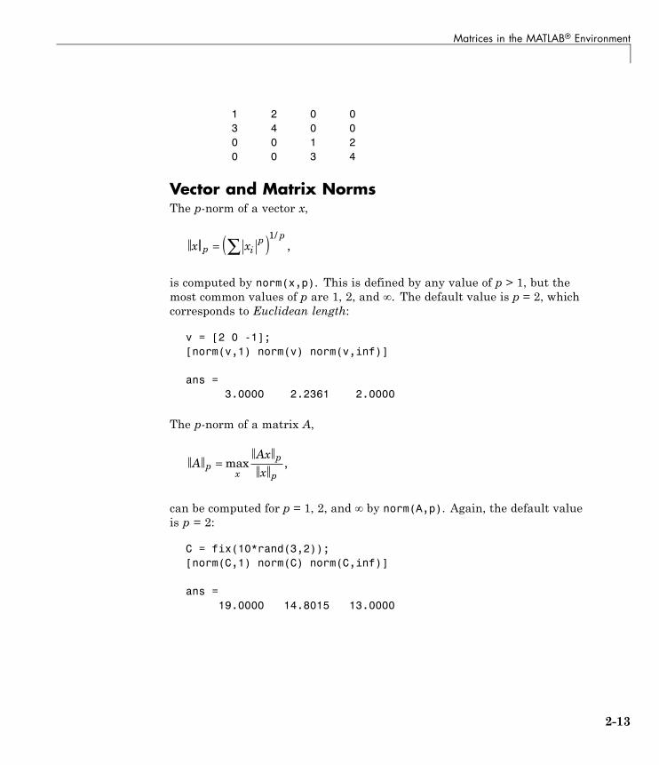
Matrices in the MATLAB® Environment
1 2 0 03 4 0 00 0 1 20 0 3 4
Vector and Matrix NormsThe p-norm of a vector x,
x xp ip p
= ( )∑1/
,
is computed by norm(x,p). This is defined by any value of p > 1, but themost common values of p are 1, 2, and ∞. The default value is p = 2, whichcorresponds to Euclidean length:
v = [2 0 -1];[norm(v,1) norm(v) norm(v,inf)]
ans =3.0000 2.2361 2.0000
The p-norm of a matrix A,
AAx
xp
x
p
p= max ,
can be computed for p = 1, 2, and ∞ by norm(A,p). Again, the default valueis p = 2:
C = fix(10*rand(3,2));[norm(C,1) norm(C) norm(C,inf)]
ans =19.0000 14.8015 13.0000
2-13
2 Linear Algebra
Using Multithreaded Computation with LinearAlgebra FunctionsMATLAB software supports multithreaded computation for a numberof linear algebra and element-wise numerical functions. These functionsautomatically execute on multiple threads. For a function or expression toexecute faster on multiple CPUs, a number of conditions must be true:
1 The function performs operations that easily partition into sections thatexecute concurrently. These sections must be able to execute with littlecommunication between processes. They should require few sequentialoperations.
2 The data size is large enough so that any advantages of concurrentexecution outweigh the time required to partition the data and manageseparate execution threads. For example, most functions speed up onlywhen the array contains than several thousand elements or more.
3 The operation is not memory-bound; processing time is not dominated bymemory access time. As a general rule, complex functions speed up morethan simple functions.
The matrix multiply (X*Y) and matrix power (X^p) operators showsignificant increase in speed on large double-precision arrays (on order of10,000 elements). The matrix analysis functions det, rcond, hess, and expmalso show significant increase in speed on large double-precision arrays.To learn more about mulithreading, see in the MATLAB ProgrammingFundamentals documentation.
2-14
Systems of Linear Equations
Systems of Linear Equations
In this section...
“Computational Considerations” on page 2-15
“The mldivide Algorithm” on page 2-17
“General Solution” on page 2-18
“Square Systems” on page 2-18
“Overdetermined Systems” on page 2-21
“Using Multithreaded Computation with Systems of Linear Equations”on page 2-24
“Iterative Methods for Solving Systems of Linear Equations” on page 2-25
Computational ConsiderationsOne of the most important problems in technical computing is the solution ofsystems of simultaneous linear equations.
In matrix notation, the general problem takes the following form: Given twomatrices A and B, does there exist a unique matrix X so that AX = B or XA = B?
It is instructive to consider a 1-by-1 example. For example, does the equation
7x = 21
have a unique solution?
The answer, of course, is yes. The equation has the unique solution x = 3. Thesolution is easily obtained by division:
x = 21/7 = 3.
The solution is not ordinarily obtained by computing the inverse of 7, that is7–1 = 0.142857..., and then multiplying 7–1 by 21. This would be more workand, if 7–1 is represented to a finite number of digits, less accurate. Similarconsiderations apply to sets of linear equations with more than one unknown;
2-15
2 Linear Algebra
the MATLAB software solves such equations without computing the inverseof the matrix.
Although it is not standard mathematical notation, MATLAB uses thedivision terminology familiar in the scalar case to describe the solution of ageneral system of simultaneous equations. The two division symbols, slash, /,and backslash, \, correspond to the two MATLAB functions mldivide andmrdivide. mldivide and mrdivide are used for the two situations where theunknown matrix appears on the left or right of the coefficient matrix:
X = B/A Denotes the solution to the matrix equationXA = B.
X = A\B Denotes the solution to the matrix equationAX = B.
Think of “dividing” both sides of the equation AX = B or XA = B by A. Thecoefficient matrix A is always in the “denominator.”
The dimension compatibility conditions for X = A\B require the two matricesA and B to have the same number of rows. The solution X then has thesame number of columns as B and its row dimension is equal to the columndimension of A. For X = B/A, the roles of rows and columns are interchanged.
In practice, linear equations of the form AX = B occur more frequently thanthose of the form XA = B. Consequently, the backslash is used far morefrequently than the slash. The remainder of this section concentrates on thebackslash operator; the corresponding properties of the slash operator canbe inferred from the identity:
(B/A)' = (A'\B')
The coefficient matrix A need not be square. If A is m-by-n, there are threecases:
2-16
Systems of Linear Equations
m = n Square system. Seek an exact solution.
m > n Overdetermined system. Find a least squaressolution.
m < n Underdetermined system. Find a basic solutionwith at most m nonzero components.
The mldivide AlgorithmThe mldivide operator employs different algorithms to handle different kindsof coefficient matrices. The various cases are diagnosed automatically byexamining the coefficient matrix.
Permutations of Triangular Matricesmldivide checks for triangularity by testing for zero elements. If a matrix Ais triangular, MATLAB software uses a substitution to compute the solutionvector x. If A is a permutation of a triangular matrix, MATLAB software usesa permuted substitution algorithm.
Square MatricesIf A is symmetric and has real, positive diagonal elements, MATLAB attemptsa Cholesky factorization. If the Cholesky factorization fails, MATLABperforms a symmetric, indefinite factorization. If A is upper Hessenberg,MATLAB uses Gaussian elimination to reduce the system to a triangularmatrix. If A is square but is neither permuted triangular, symmetric andpositive definite, or Hessenberg, MATLAB performs a general triangularfactorization using LU factorization with partial pivoting (see lu).
Rectangular MatricesIf A is rectangular, mldivide returns a least-squares solution. MATLABsolves overdetermined systems with QR factorization (see qr). For anunderdetermined system, MATLAB returns the solution with the maximumnumber of zero elements.
The mldivide function reference page contains a more detailed descriptionof the algorithm.
2-17
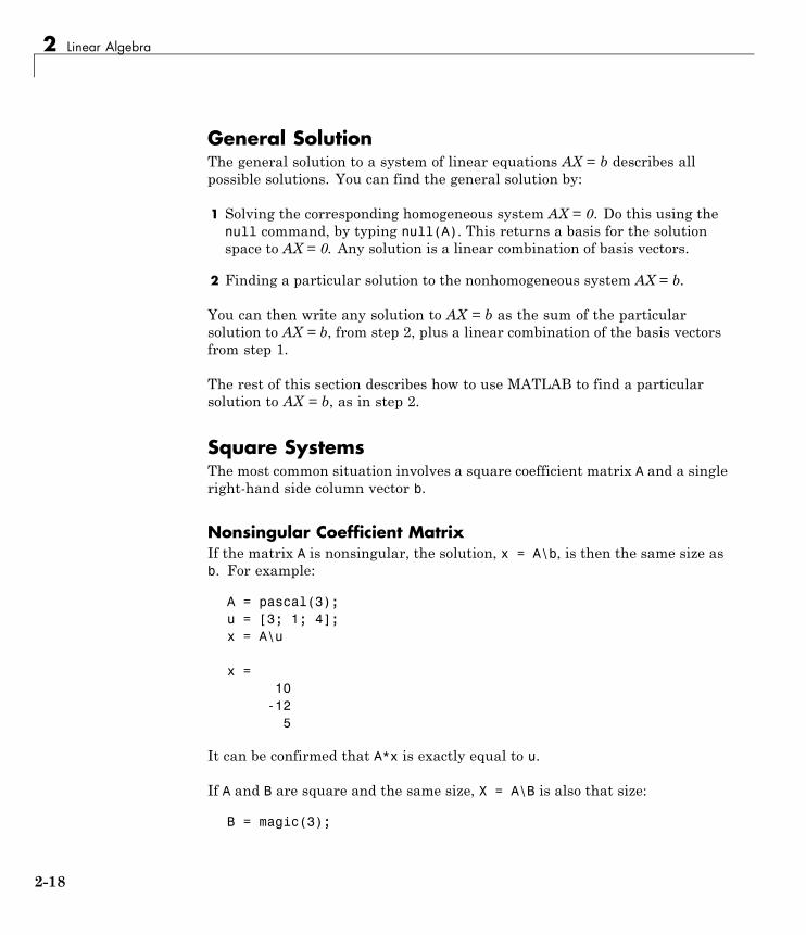
2 Linear Algebra
General SolutionThe general solution to a system of linear equations AX = b describes allpossible solutions. You can find the general solution by:
1 Solving the corresponding homogeneous system AX = 0. Do this using thenull command, by typing null(A). This returns a basis for the solutionspace to AX = 0. Any solution is a linear combination of basis vectors.
2 Finding a particular solution to the nonhomogeneous system AX = b.
You can then write any solution to AX = b as the sum of the particularsolution to AX = b, from step 2, plus a linear combination of the basis vectorsfrom step 1.
The rest of this section describes how to use MATLAB to find a particularsolution to AX = b, as in step 2.
Square SystemsThe most common situation involves a square coefficient matrix A and a singleright-hand side column vector b.
Nonsingular Coefficient MatrixIf the matrix A is nonsingular, the solution, x = A\b, is then the same size asb. For example:
A = pascal(3);u = [3; 1; 4];x = A\u
x =10
-125
It can be confirmed that A*x is exactly equal to u.
If A and B are square and the same size, X = A\B is also that size:
B = magic(3);
2-18
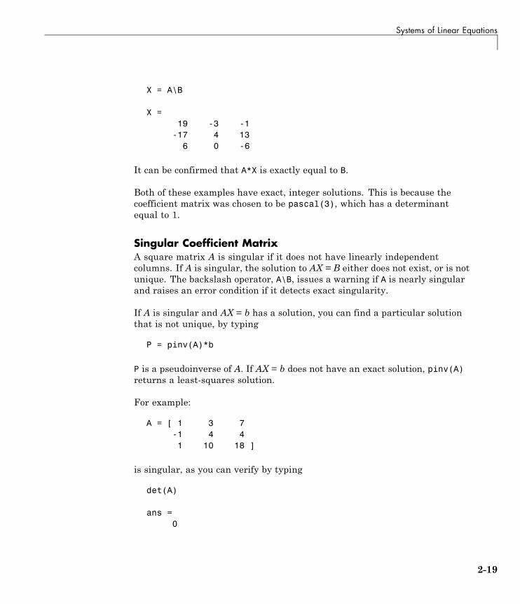
Systems of Linear Equations
X = A\B
X =19 -3 -1
-17 4 136 0 -6
It can be confirmed that A*X is exactly equal to B.
Both of these examples have exact, integer solutions. This is because thecoefficient matrix was chosen to be pascal(3), which has a determinantequal to 1.
Singular Coefficient MatrixA square matrix A is singular if it does not have linearly independentcolumns. If A is singular, the solution to AX = B either does not exist, or is notunique. The backslash operator, A\B, issues a warning if A is nearly singularand raises an error condition if it detects exact singularity.
If A is singular and AX = b has a solution, you can find a particular solutionthat is not unique, by typing
P = pinv(A)*b
P is a pseudoinverse of A. If AX = b does not have an exact solution, pinv(A)returns a least-squares solution.
For example:
A = [ 1 3 7-1 4 41 10 18 ]
is singular, as you can verify by typing
det(A)
ans =0
2-19
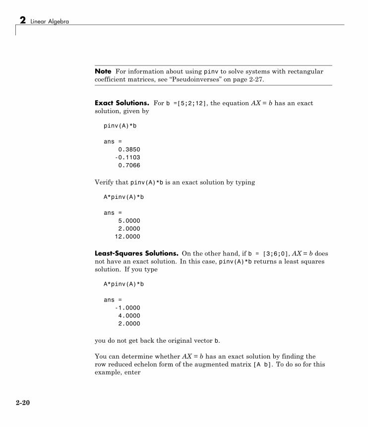
2 Linear Algebra
Note For information about using pinv to solve systems with rectangularcoefficient matrices, see “Pseudoinverses” on page 2-27.
Exact Solutions. For b =[5;2;12], the equation AX = b has an exactsolution, given by
pinv(A)*b
ans =0.3850
-0.11030.7066
Verify that pinv(A)*b is an exact solution by typing
A*pinv(A)*b
ans =5.00002.0000
12.0000
Least-Squares Solutions. On the other hand, if b = [3;6;0], AX = b doesnot have an exact solution. In this case, pinv(A)*b returns a least squaressolution. If you type
A*pinv(A)*b
ans =-1.00004.00002.0000
you do not get back the original vector b.
You can determine whether AX = b has an exact solution by finding therow reduced echelon form of the augmented matrix [A b]. To do so for thisexample, enter
2-20
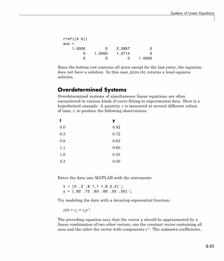
Systems of Linear Equations
rref([A b])ans =
1.0000 0 2.2857 00 1.0000 1.5714 00 0 0 1.0000
Since the bottom row contains all zeros except for the last entry, the equationdoes not have a solution. In this case, pinv(A) returns a least-squaressolution.
Overdetermined SystemsOverdetermined systems of simultaneous linear equations are oftenencountered in various kinds of curve fitting to experimental data. Here is ahypothetical example. A quantity y is measured at several different valuesof time, t, to produce the following observations:
t y
0.0 0.82
0.3 0.72
0.8 0.63
1.1 0.60
1.6 0.55
2.3 0.50
Enter the data into MATLAB with the statements
t = [0 .3 .8 1.1 1.6 2.3]';y = [.82 .72 .63 .60 .55 .50]';
Try modeling the data with a decaying exponential function:
y(t) = c1 + c2e–t.
The preceding equation says that the vector y should be approximated by alinear combination of two other vectors, one the constant vector containing allones and the other the vector with components e–t. The unknown coefficients,
2-21
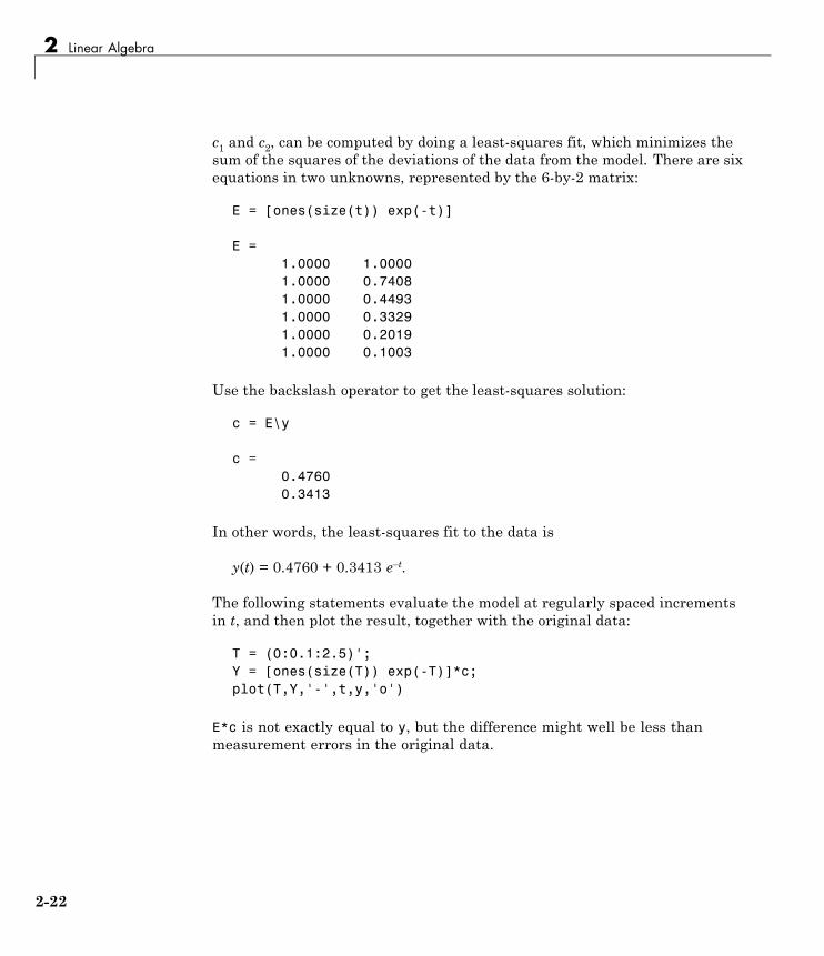
2 Linear Algebra
c1 and c2, can be computed by doing a least-squares fit, which minimizes thesum of the squares of the deviations of the data from the model. There are sixequations in two unknowns, represented by the 6-by-2 matrix:
E = [ones(size(t)) exp(-t)]
E =1.0000 1.00001.0000 0.74081.0000 0.44931.0000 0.33291.0000 0.20191.0000 0.1003
Use the backslash operator to get the least-squares solution:
c = E\y
c =0.47600.3413
In other words, the least-squares fit to the data is
y(t) = 0.4760 + 0.3413 e–t.
The following statements evaluate the model at regularly spaced incrementsin t, and then plot the result, together with the original data:
T = (0:0.1:2.5)';Y = [ones(size(T)) exp(-T)]*c;plot(T,Y,'-',t,y,'o')
E*c is not exactly equal to y, but the difference might well be less thanmeasurement errors in the original data.
2-22
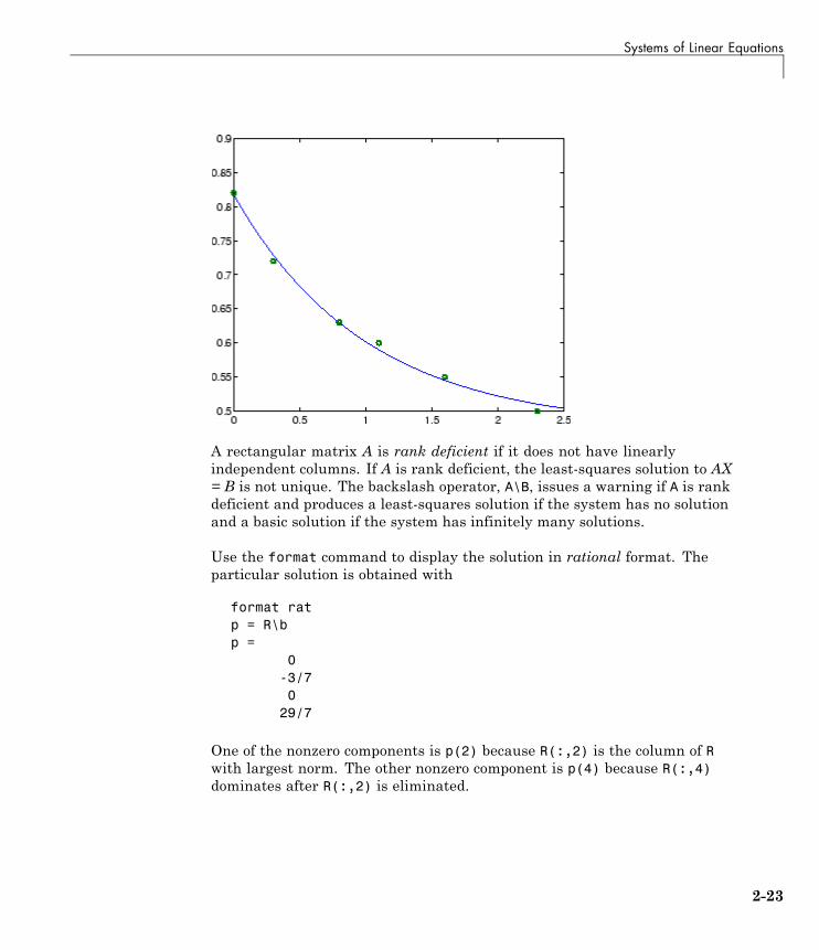
Systems of Linear Equations
A rectangular matrix A is rank deficient if it does not have linearlyindependent columns. If A is rank deficient, the least-squares solution to AX= B is not unique. The backslash operator, A\B, issues a warning if A is rankdeficient and produces a least-squares solution if the system has no solutionand a basic solution if the system has infinitely many solutions.
Use the format command to display the solution in rational format. Theparticular solution is obtained with
format ratp = R\bp =
0-3/70
29/7
One of the nonzero components is p(2) because R(:,2) is the column of Rwith largest norm. The other nonzero component is p(4) because R(:,4)dominates after R(:,2) is eliminated.
2-23
2 Linear Algebra
The complete solution to the underdetermined system can be characterized byadding an arbitrary vector from the null space, which can be found using thenull function with an option requesting a rational basis:
Z = null(R,'r')Z =
-1/2 -7/6-1/2 1/21 00 1
It can be confirmed that R*Z is zero and that any vector x where
x = p + Z*q
for an arbitrary vector q satisfies R*x = b.
Using Multithreaded Computation with Systems ofLinear EquationsMATLAB software supports multithreaded computation for a numberof linear algebra and element-wise numerical functions. These functionsautomatically execute on multiple threads. For a function or expression toexecute faster on multiple CPUs, a number of conditions must be true:
1 The function performs operations that easily partition into sections thatexecute concurrently. These sections must be able to execute with littlecommunication between processes. They should require few sequentialoperations.
2 The data size is large enough so that any advantages of concurrentexecution outweigh the time required to partition the data and manageseparate execution threads. For example, most functions speed up onlywhen the array contains than several thousand elements or more.
3 The operation is not memory-bound; processing time is not dominated bymemory access time. As a general rule, complex functions speed up morethan simple functions.
inv, lscov, linsolve, and mldivide show significant increase in speed onlarge double-precision arrays (on order of 10,000 elements or more) when
2-24
Systems of Linear Equations
multithreading is enabled. To learn more about mulithreading, see in theMATLAB Programming Fundamentals documentation.
Iterative Methods for Solving Systems of LinearEquationsIf the coefficient matrix A is large and sparse, factorization methods aregenerally not efficient. Iterative methods generate a series of approximatesolutions. MATLAB provides several iterative methods to handle large,sparse input matrices.
pcgPreconditioned conjugate gradients method. This method is appropriatefor Hermitian positive definite coefficient matrix A.
bicgBiConjugate Gradients Method
bicgstabBiConjugate Gradients Stabilized Method
bicgstablBiCGStab(l) Method
cgsConjugate Gradients Squared Method
gmresGeneralized Minimum Residual Method
lsqrLSQR Method
minresMinimum Residual Method. This method is appropriate for Hermitiancoefficient matrix A.
qmrQuasi-Minimal Residual Method
symmlqSymmetric LQ Method
tfqmrTranspose-Free QMR Method
2-25
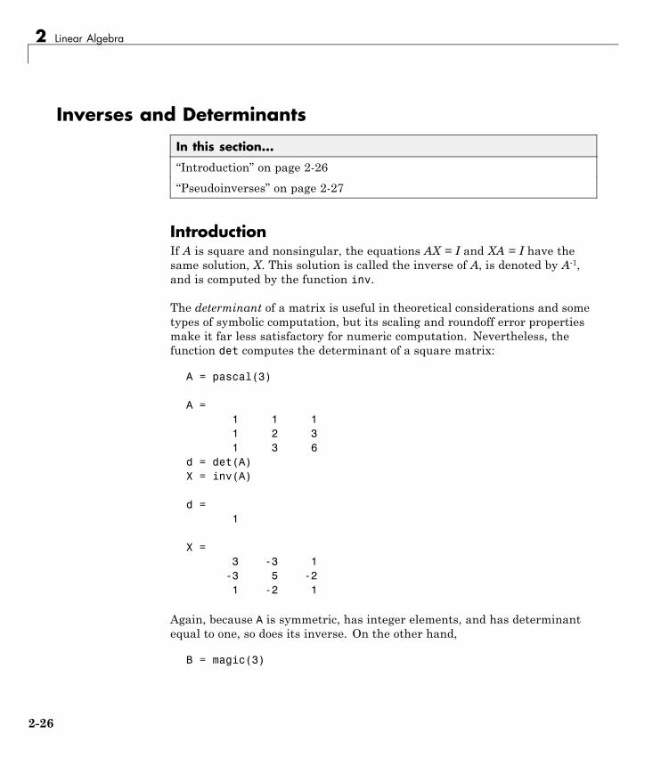
2 Linear Algebra
Inverses and Determinants
In this section...
“Introduction” on page 2-26
“Pseudoinverses” on page 2-27
IntroductionIf A is square and nonsingular, the equations AX = I and XA = I have thesame solution, X. This solution is called the inverse of A, is denoted by A-1,and is computed by the function inv.
The determinant of a matrix is useful in theoretical considerations and sometypes of symbolic computation, but its scaling and roundoff error propertiesmake it far less satisfactory for numeric computation. Nevertheless, thefunction det computes the determinant of a square matrix:
A = pascal(3)
A =1 1 11 2 31 3 6
d = det(A)X = inv(A)
d =1
X =3 -3 1
-3 5 -21 -2 1
Again, because A is symmetric, has integer elements, and has determinantequal to one, so does its inverse. On the other hand,
B = magic(3)
2-26
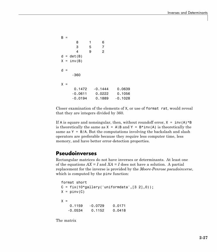
Inverses and Determinants
B =8 1 63 5 74 9 2
d = det(B)X = inv(B)
d =-360
X =0.1472 -0.1444 0.0639
-0.0611 0.0222 0.1056-0.0194 0.1889 -0.1028
Closer examination of the elements of X, or use of format rat, would revealthat they are integers divided by 360.
If A is square and nonsingular, then, without roundoff error, X = inv(A)*Bis theoretically the same as X = A\B and Y = B*inv(A) is theoretically thesame as Y = B/A. But the computations involving the backslash and slashoperators are preferable because they require less computer time, lessmemory, and have better error-detection properties.
PseudoinversesRectangular matrices do not have inverses or determinants. At least oneof the equations AX = I and XA = I does not have a solution. A partialreplacement for the inverse is provided by the Moore-Penrose pseudoinverse,which is computed by the pinv function:
format shortC = fix(10*gallery('uniformdata',[3 2],0));X = pinv(C)
X =0.1159 -0.0729 0.0171
-0.0534 0.1152 0.0418
The matrix
2-27
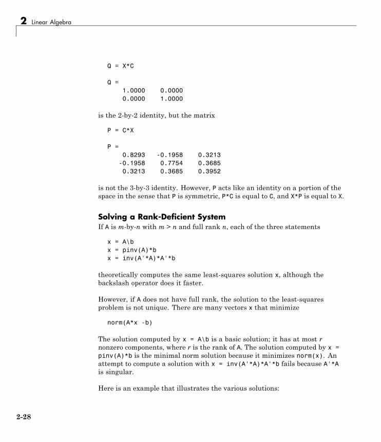
2 Linear Algebra
Q = X*C
Q =1.0000 0.00000.0000 1.0000
is the 2-by-2 identity, but the matrix
P = C*X
P =0.8293 -0.1958 0.3213
-0.1958 0.7754 0.36850.3213 0.3685 0.3952
is not the 3-by-3 identity. However, P acts like an identity on a portion of thespace in the sense that P is symmetric, P*C is equal to C, and X*P is equal to X.
Solving a Rank-Deficient SystemIf A is m-by-n with m > n and full rank n, each of the three statements
x = A\bx = pinv(A)*bx = inv(A'*A)*A'*b
theoretically computes the same least-squares solution x, although thebackslash operator does it faster.
However, if A does not have full rank, the solution to the least-squaresproblem is not unique. There are many vectors x that minimize
norm(A*x -b)
The solution computed by x = A\b is a basic solution; it has at most rnonzero components, where r is the rank of A. The solution computed by x =pinv(A)*b is the minimal norm solution because it minimizes norm(x). Anattempt to compute a solution with x = inv(A'*A)*A'*b fails because A'*Ais singular.
Here is an example that illustrates the various solutions:
2-28
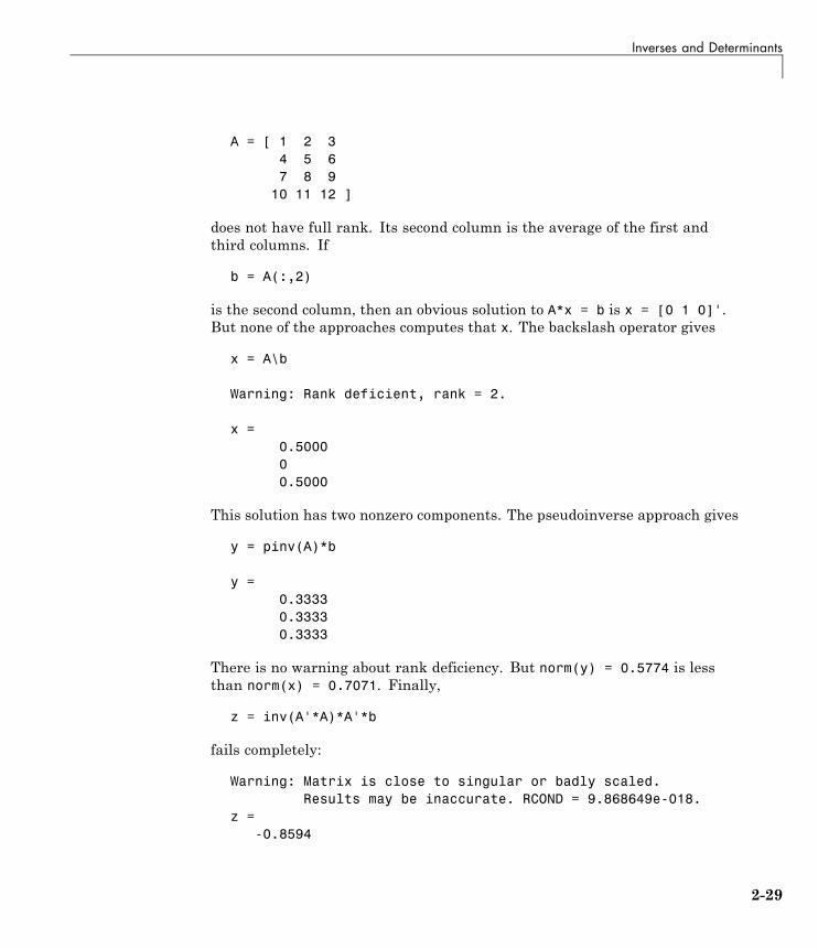
Inverses and Determinants
A = [ 1 2 34 5 67 8 9
10 11 12 ]
does not have full rank. Its second column is the average of the first andthird columns. If
b = A(:,2)
is the second column, then an obvious solution to A*x = b is x = [0 1 0]'.But none of the approaches computes that x. The backslash operator gives
x = A\b
Warning: Rank deficient, rank = 2.
x =0.500000.5000
This solution has two nonzero components. The pseudoinverse approach gives
y = pinv(A)*b
y =0.33330.33330.3333
There is no warning about rank deficiency. But norm(y) = 0.5774 is lessthan norm(x) = 0.7071. Finally,
z = inv(A'*A)*A'*b
fails completely:
Warning: Matrix is close to singular or badly scaled.Results may be inaccurate. RCOND = 9.868649e-018.
z =-0.8594
2-29

2 Linear Algebra
1.3438-0.6875
2-30

Factorizations
Factorizations
In this section...
“Introduction” on page 2-31
“Cholesky Factorization” on page 2-31
“LU Factorization” on page 2-33
“QR Factorization” on page 2-34
“Using Multithreaded Computation for Factorization” on page 2-38
IntroductionAll three of the matrix factorizations discussed in this section make use oftriangularmatrices, where all the elements either above or below the diagonalare zero. Systems of linear equations involving triangular matrices are easilyand quickly solved using either forward or back substitution.
Cholesky FactorizationThe Cholesky factorization expresses a symmetric matrix as the product of atriangular matrix and its transpose
A = R’R,
where R is an upper triangular matrix.
Not all symmetric matrices can be factored in this way; the matrices thathave such a factorization are said to be positive definite. This implies thatall the diagonal elements of A are positive and that the offdiagonal elementsare “not too big.” The Pascal matrices provide an interesting example.Throughout this chapter, the example matrix A has been the 3-by-3 Pascalmatrix. Temporarily switch to the 6-by-6:
A = pascal(6)
A =1 1 1 1 1 11 2 3 4 5 6
2-31

2 Linear Algebra
1 3 6 10 15 211 4 10 20 35 561 5 15 35 70 1261 6 21 56 126 252
The elements of A are binomial coefficients. Each element is the sum of itsnorth and west neighbors. The Cholesky factorization is
R = chol(A)
R =1 1 1 1 1 10 1 2 3 4 50 0 1 3 6 100 0 0 1 4 100 0 0 0 1 50 0 0 0 0 1
The elements are again binomial coefficients. The fact that R'*R is equal to Ademonstrates an identity involving sums of products of binomial coefficients.
Note The Cholesky factorization also applies to complex matrices. Anycomplex matrix that has a Cholesky factorization satisfies A’ = A and is saidto be Hermitian positive definite.
The Cholesky factorization allows the linear system
Ax = b
to be replaced by
R’Rx = b.
Because the backslash operator recognizes triangular systems, this can besolved in the MATLAB environment quickly with
x = R\(R'\b)
2-32
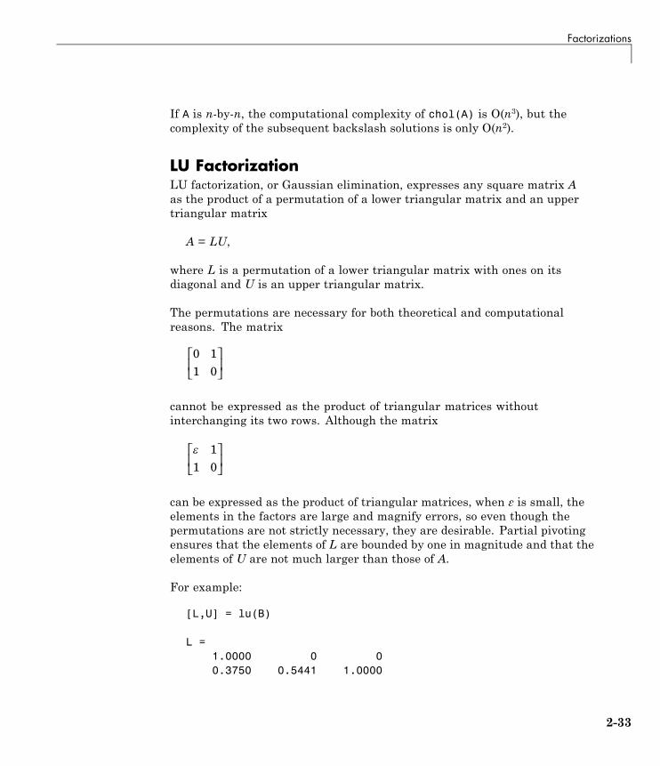
Factorizations
If A is n-by-n, the computational complexity of chol(A) is O(n3), but thecomplexity of the subsequent backslash solutions is only O(n2).
LU FactorizationLU factorization, or Gaussian elimination, expresses any square matrix Aas the product of a permutation of a lower triangular matrix and an uppertriangular matrix
A = LU,
where L is a permutation of a lower triangular matrix with ones on itsdiagonal and U is an upper triangular matrix.
The permutations are necessary for both theoretical and computationalreasons. The matrix
0 11 0
⎡
⎣⎢
⎤
⎦⎥
cannot be expressed as the product of triangular matrices withoutinterchanging its two rows. Although the matrix
11 0
⎡
⎣⎢
⎤
⎦⎥
can be expressed as the product of triangular matrices, when ε is small, theelements in the factors are large and magnify errors, so even though thepermutations are not strictly necessary, they are desirable. Partial pivotingensures that the elements of L are bounded by one in magnitude and that theelements of U are not much larger than those of A.
For example:
[L,U] = lu(B)
L =1.0000 0 00.3750 0.5441 1.0000
2-33
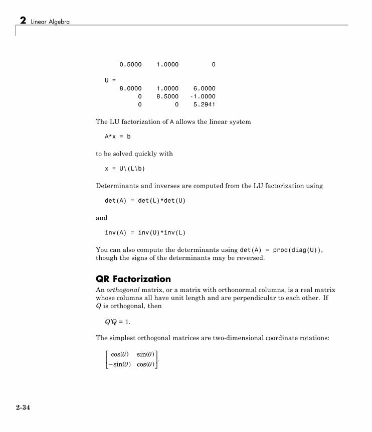
2 Linear Algebra
0.5000 1.0000 0
U =8.0000 1.0000 6.0000
0 8.5000 -1.00000 0 5.2941
The LU factorization of A allows the linear system
A*x = b
to be solved quickly with
x = U\(L\b)
Determinants and inverses are computed from the LU factorization using
det(A) = det(L)*det(U)
and
inv(A) = inv(U)*inv(L)
You can also compute the determinants using det(A) = prod(diag(U)),though the signs of the determinants may be reversed.
QR FactorizationAn orthogonal matrix, or a matrix with orthonormal columns, is a real matrixwhose columns all have unit length and are perpendicular to each other. IfQ is orthogonal, then
Q’Q = 1.
The simplest orthogonal matrices are two-dimensional coordinate rotations:
cos( ) sin( )sin( ) cos( )
. −
⎡
⎣⎢
⎤
⎦⎥
2-34
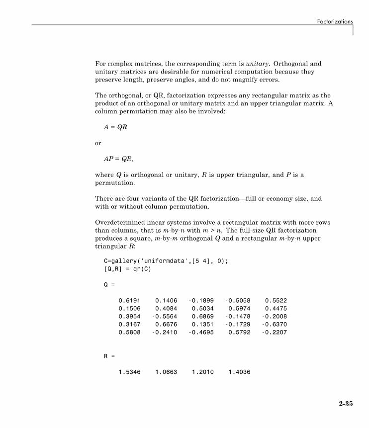
Factorizations
For complex matrices, the corresponding term is unitary. Orthogonal andunitary matrices are desirable for numerical computation because theypreserve length, preserve angles, and do not magnify errors.
The orthogonal, or QR, factorization expresses any rectangular matrix as theproduct of an orthogonal or unitary matrix and an upper triangular matrix. Acolumn permutation may also be involved:
A = QR
or
AP = QR,
where Q is orthogonal or unitary, R is upper triangular, and P is apermutation.
There are four variants of the QR factorization—full or economy size, andwith or without column permutation.
Overdetermined linear systems involve a rectangular matrix with more rowsthan columns, that is m-by-n with m > n. The full-size QR factorizationproduces a square, m-by-m orthogonal Q and a rectangular m-by-n uppertriangular R:
C=gallery('uniformdata',[5 4], 0);[Q,R] = qr(C)
Q =
0.6191 0.1406 -0.1899 -0.5058 0.55220.1506 0.4084 0.5034 0.5974 0.44750.3954 -0.5564 0.6869 -0.1478 -0.20080.3167 0.6676 0.1351 -0.1729 -0.63700.5808 -0.2410 -0.4695 0.5792 -0.2207
R =
1.5346 1.0663 1.2010 1.4036
2-35
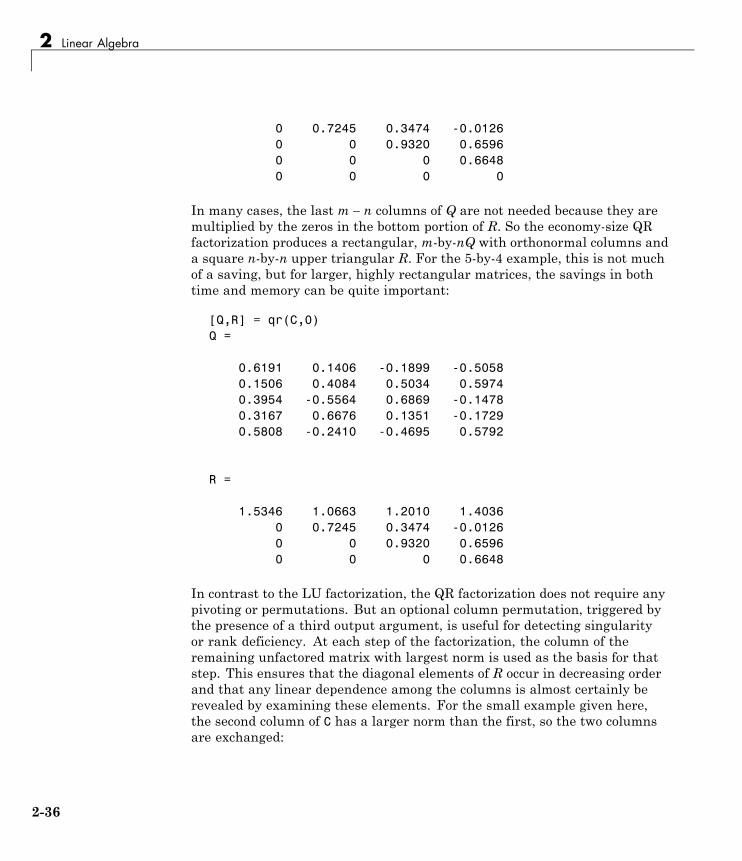
2 Linear Algebra
0 0.7245 0.3474 -0.01260 0 0.9320 0.65960 0 0 0.66480 0 0 0
In many cases, the last m – n columns of Q are not needed because they aremultiplied by the zeros in the bottom portion of R. So the economy-size QRfactorization produces a rectangular, m-by-nQ with orthonormal columns anda square n-by-n upper triangular R. For the 5-by-4 example, this is not muchof a saving, but for larger, highly rectangular matrices, the savings in bothtime and memory can be quite important:
[Q,R] = qr(C,0)Q =
0.6191 0.1406 -0.1899 -0.50580.1506 0.4084 0.5034 0.59740.3954 -0.5564 0.6869 -0.14780.3167 0.6676 0.1351 -0.17290.5808 -0.2410 -0.4695 0.5792
R =
1.5346 1.0663 1.2010 1.40360 0.7245 0.3474 -0.01260 0 0.9320 0.65960 0 0 0.6648
In contrast to the LU factorization, the QR factorization does not require anypivoting or permutations. But an optional column permutation, triggered bythe presence of a third output argument, is useful for detecting singularityor rank deficiency. At each step of the factorization, the column of theremaining unfactored matrix with largest norm is used as the basis for thatstep. This ensures that the diagonal elements of R occur in decreasing orderand that any linear dependence among the columns is almost certainly berevealed by examining these elements. For the small example given here,the second column of C has a larger norm than the first, so the two columnsare exchanged:
2-36
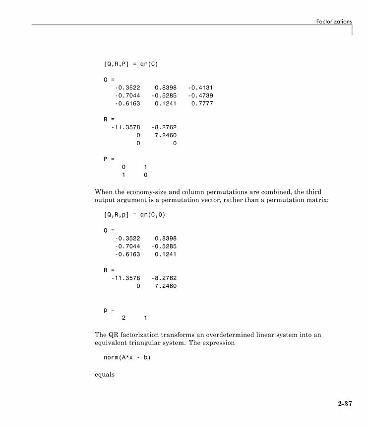
Factorizations
[Q,R,P] = qr(C)
Q =-0.3522 0.8398 -0.4131-0.7044 -0.5285 -0.4739-0.6163 0.1241 0.7777
R =-11.3578 -8.2762
0 7.24600 0
P =0 11 0
When the economy-size and column permutations are combined, the thirdoutput argument is a permutation vector, rather than a permutation matrix:
[Q,R,p] = qr(C,0)
Q =-0.3522 0.8398-0.7044 -0.5285-0.6163 0.1241
R =-11.3578 -8.2762
0 7.2460
p =2 1
The QR factorization transforms an overdetermined linear system into anequivalent triangular system. The expression
norm(A*x - b)
equals
2-37
2 Linear Algebra
norm(Q*R*x - b)
Multiplication by orthogonal matrices preserves the Euclidean norm, so thisexpression is also equal to
norm(R*x - y)
where y = Q'*b. Since the last m-n rows of R are zero, this expression breaksinto two pieces:
norm(R(1:n,1:n)*x - y(1:n))
and
norm(y(n+1:m))
When A has full rank, it is possible to solve for x so that the first of theseexpressions is zero. Then the second expression gives the norm of the residual.When A does not have full rank, the triangular structure of Rmakes it possibleto find a basic solution to the least-squares problem.
Using Multithreaded Computation for FactorizationMATLAB software supports multithreaded computation for a numberof linear algebra and element-wise numerical functions. These functionsautomatically execute on multiple threads. For a function or expression toexecute faster on multiple CPUs, a number of conditions must be true:
1 The function performs operations that easily partition into sections thatexecute concurrently. These sections must be able to execute with littlecommunication between processes. They should require few sequentialoperations.
2 The data size is large enough so that any advantages of concurrentexecution outweigh the time required to partition the data and manageseparate execution threads. For example, most functions speed up onlywhen the array contains several thousand elements or more.
3 The operation is not memory-bound; processing time is not dominated bymemory access time. As a general rule, complex functions speed up morethan simple functions.
2-38
Factorizations
lu and qr show significant increase in speed on large double-precision arrays(on order of 10,000 elements). To learn more about mulithreading, see in theMATLAB Programming Fundamentals documentation.
2-39
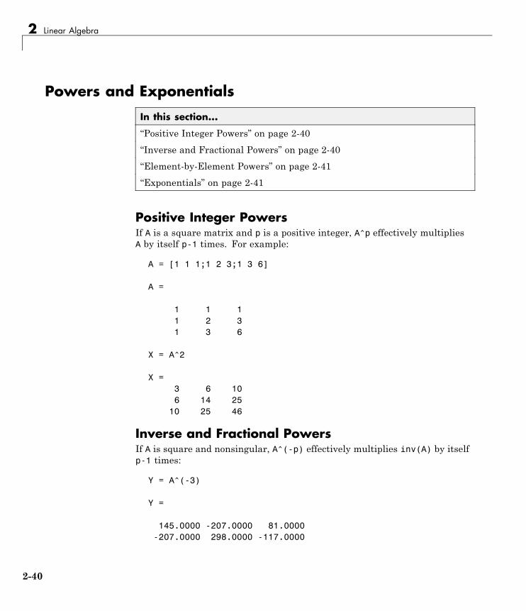
2 Linear Algebra
Powers and Exponentials
In this section...
“Positive Integer Powers” on page 2-40
“Inverse and Fractional Powers” on page 2-40
“Element-by-Element Powers” on page 2-41
“Exponentials” on page 2-41
Positive Integer PowersIf A is a square matrix and p is a positive integer, A^p effectively multipliesA by itself p-1 times. For example:
A = [1 1 1;1 2 3;1 3 6]
A =
1 1 11 2 31 3 6
X = A^2
X =3 6 106 14 25
10 25 46
Inverse and Fractional PowersIf A is square and nonsingular, A^(-p) effectively multiplies inv(A) by itselfp-1 times:
Y = A^(-3)
Y =
145.0000 -207.0000 81.0000-207.0000 298.0000 -117.0000
2-40
Powers and Exponentials
81.0000 -117.0000 46.0000
Fractional powers, like A^(2/3), are also permitted; the results depend uponthe distribution of the eigenvalues of the matrix.
Element-by-Element PowersThe .^ operator produces element-by-element powers. For example:
X = A.^2
A =1 1 11 4 91 9 36
ExponentialsThe function
sqrtm(A)
computes A^(1/2) by a more accurate algorithm. The m in sqrtm distinguishesthis function from sqrt(A), which, like A.^(1/2), does its job element byelement.
A system of linear, constant coefficient, ordinary differential equations can bewritten
dx/dt = Ax,
where x = x(t) is a vector of functions of t and A is a matrix independent of t.The solution can be expressed in terms of the matrix exponential:
x(t) = etAx(0).
The function
expm(A)
computes the matrix exponential. An example is provided by the 3-by-3coefficient matrix
2-41
2 Linear Algebra
A =0 -6 -16 2 -16
-5 20 -10
and the initial condition, x(0)
x0 =111
The matrix exponential is used to compute the solution, x(t), to the differentialequation at 101 points on the interval 0 ≤ t ≤ 1 with
X = [];for t = 0:.01:1
X = [X expm(t*A)*x0];end
A three-dimensional phase plane plot obtained with
plot3(X(1,:),X(2,:),X(3,:),'-o')
shows the solution spiraling in towards the origin. This behavior is relatedto the eigenvalues of the coefficient matrix, which are discussed in the nextsection.
2-42
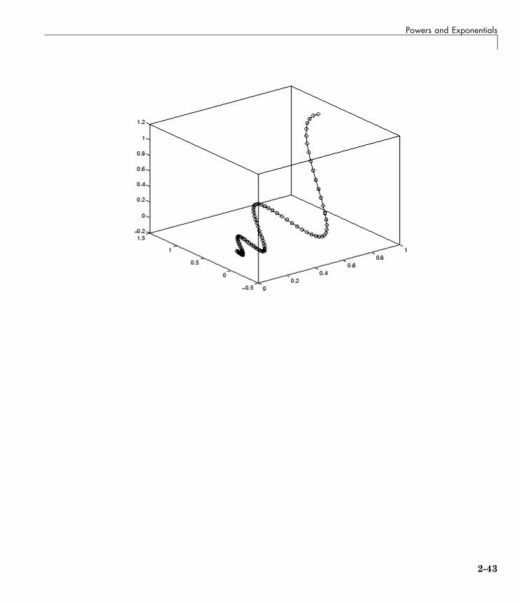
Powers and Exponentials
2-43
2 Linear Algebra
Eigenvalues
In this section...
“Eigenvalue Decomposition” on page 2-44
“Multiple Eigenvalues” on page 2-45
“Schur Decomposition” on page 2-46
Eigenvalue DecompositionAn eigenvalue and eigenvector of a square matrix A are, respectively, a scalarλ and a nonzero vector v that satisfy
Aυ = λυ.
With the eigenvalues on the diagonal of a diagonal matrix Λ and thecorresponding eigenvectors forming the columns of a matrix V, you have
AV = VΛ.
If V is nonsingular, this becomes the eigenvalue decomposition
A = VΛV–1.
A good example is provided by the coefficient matrix of the ordinarydifferential equation in the previous section:
A =0 -6 -16 2 -16
-5 20 -10
The statement
lambda = eig(A)
produces a column vector containing the eigenvalues. For this matrix, theeigenvalues are complex:
lambda =
2-44
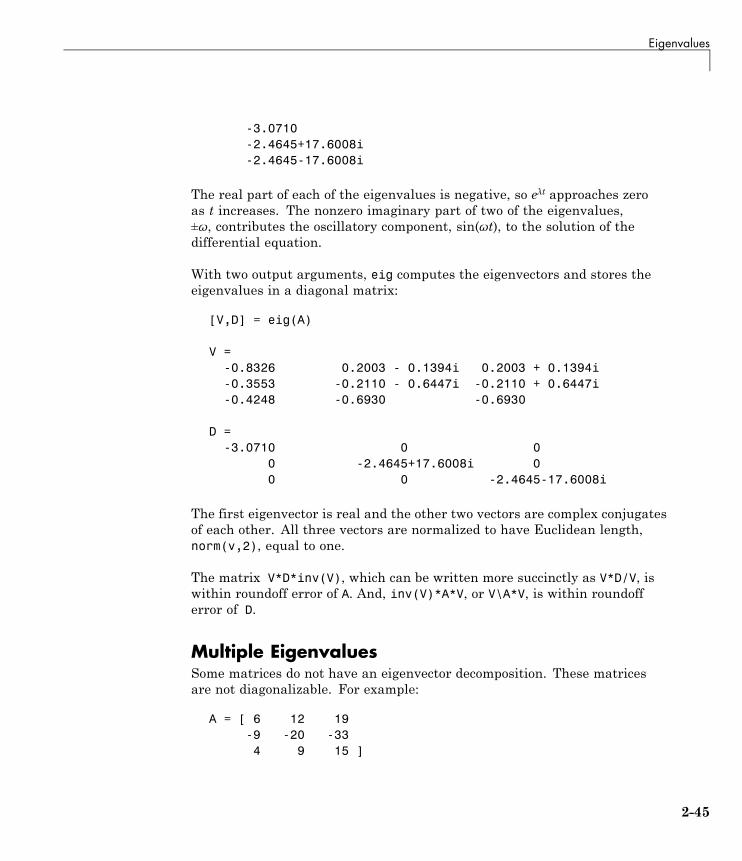
Eigenvalues
-3.0710-2.4645+17.6008i-2.4645-17.6008i
The real part of each of the eigenvalues is negative, so eλt approaches zeroas t increases. The nonzero imaginary part of two of the eigenvalues,±ω, contributes the oscillatory component, sin(ωt), to the solution of thedifferential equation.
With two output arguments, eig computes the eigenvectors and stores theeigenvalues in a diagonal matrix:
[V,D] = eig(A)
V =-0.8326 0.2003 - 0.1394i 0.2003 + 0.1394i-0.3553 -0.2110 - 0.6447i -0.2110 + 0.6447i-0.4248 -0.6930 -0.6930
D =-3.0710 0 0
0 -2.4645+17.6008i 00 0 -2.4645-17.6008i
The first eigenvector is real and the other two vectors are complex conjugatesof each other. All three vectors are normalized to have Euclidean length,norm(v,2), equal to one.
The matrix V*D*inv(V), which can be written more succinctly as V*D/V, iswithin roundoff error of A. And, inv(V)*A*V, or V\A*V, is within roundofferror of D.
Multiple EigenvaluesSome matrices do not have an eigenvector decomposition. These matricesare not diagonalizable. For example:
A = [ 6 12 19-9 -20 -334 9 15 ]
2-45
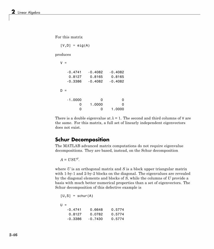
2 Linear Algebra
For this matrix
[V,D] = eig(A)
produces
V =
-0.4741 -0.4082 -0.40820.8127 0.8165 0.8165
-0.3386 -0.4082 -0.4082
D =
-1.0000 0 00 1.0000 00 0 1.0000
There is a double eigenvalue at λ = 1. The second and third columns of V arethe same. For this matrix, a full set of linearly independent eigenvectorsdoes not exist.
Schur DecompositionThe MATLAB advanced matrix computations do not require eigenvaluedecompositions. They are based, instead, on the Schur decomposition
A = USUT.
where U is an orthogonal matrix and S is a block upper triangular matrixwith 1-by-1 and 2-by-2 blocks on the diagonal. The eigenvalues are revealedby the diagonal elements and blocks of S, while the columns of U provide abasis with much better numerical properties than a set of eigenvectors. TheSchur decomposition of this defective example is
[U,S] = schur(A)
U =-0.4741 0.6648 0.57740.8127 0.0782 0.5774
-0.3386 -0.7430 0.5774
2-46

Eigenvalues
S =-1.0000 20.7846 -44.6948
0 1.0000 -0.60960 0 1.0000
The double eigenvalue is contained in the lower 2-by-2 block of S.
Note If A is complex, schur returns the complex Schur form, which is uppertriangular with the eigenvalues of A on the diagonal.
2-47
2 Linear Algebra
Singular ValuesA singular value and corresponding singular vectors of a rectangular matrix Aare, respectively, a scalar σ and a pair of vectors u and v that satisfy
Av = σuATu = σv.
With the singular values on the diagonal of a diagonal matrix Σ and thecorresponding singular vectors forming the columns of two orthogonalmatrices U and V, you have
AV = UΣATU = VΣ.
Since U and V are orthogonal, this becomes the singular value decomposition
A = UΣVT.
The full singular value decomposition of anm-by-nmatrix involves an m-by-mU, an m-by-n Σ, and an n-by-n V. In other words, U and V are both square andΣ is the same size as A. If A has many more rows than columns, the resultingU can be quite large, but most of its columns are multiplied by zeros in Σ. Inthis situation, the economy sized decomposition saves both time and storageby producing an m-by-n U, an n-by-n Σ and the same V.
The eigenvalue decomposition is the appropriate tool for analyzing a matrixwhen it represents a mapping from a vector space into itself, as it does foran ordinary differential equation. On the other hand, the singular valuedecomposition is the appropriate tool for analyzing a mapping from one vectorspace into another vector space, possibly with a different dimension. Mostsystems of simultaneous linear equations fall into this second category.
If A is square, symmetric, and positive definite, then its eigenvalue andsingular value decompositions are the same. But, as A departs from symmetryand positive definiteness, the difference between the two decompositionsincreases. In particular, the singular value decomposition of a real matrixis always real, but the eigenvalue decomposition of a real, nonsymmetricmatrix might be complex.
2-48
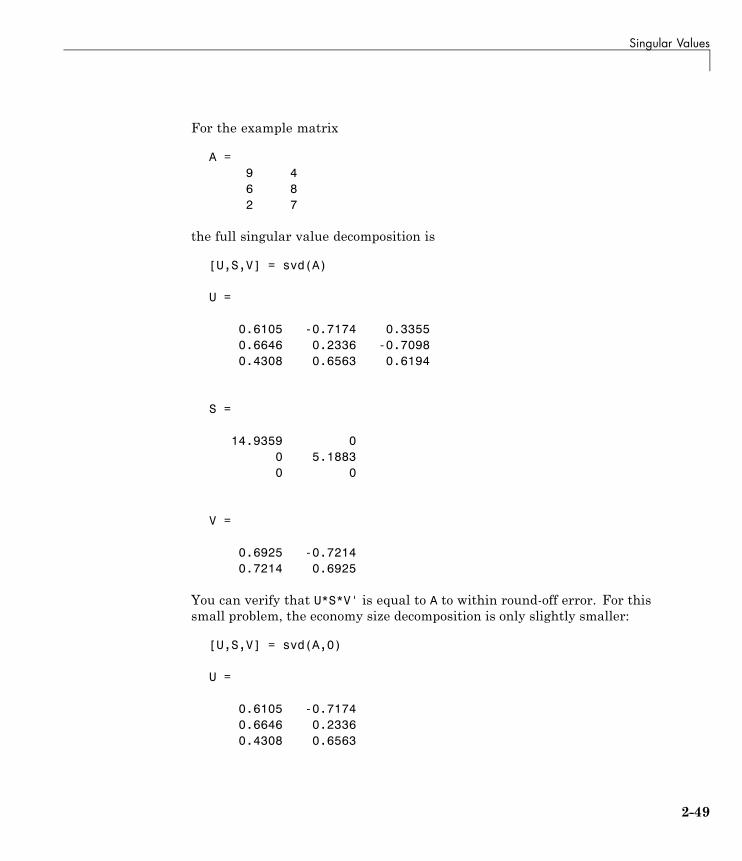
Singular Values
For the example matrix
A =9 46 82 7
the full singular value decomposition is
[U,S,V] = svd(A)
U =
0.6105 -0.7174 0.33550.6646 0.2336 -0.70980.4308 0.6563 0.6194
S =
14.9359 00 5.18830 0
V =
0.6925 -0.72140.7214 0.6925
You can verify that U*S*V' is equal to A to within round-off error. For thissmall problem, the economy size decomposition is only slightly smaller:
[U,S,V] = svd(A,0)
U =
0.6105 -0.71740.6646 0.23360.4308 0.6563
2-49
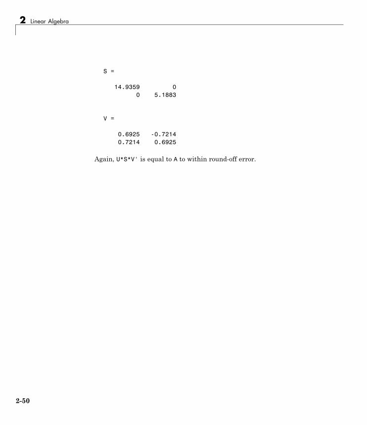
2 Linear Algebra
S =
14.9359 00 5.1883
V =
0.6925 -0.72140.7214 0.6925
Again, U*S*V' is equal to A to within round-off error.
2-50
3
Random Numbers
• “Generating Random Numbers” on page 3-2
• “Managing the Default Stream” on page 3-3
• “Creating and Controlling a Random Number Stream” on page 3-10
• “Multiple streams” on page 3-19
• “Updating Your Random Number Generator Syntax” on page 3-22
• “Selected Bibliography” on page 3-26
Pseudorandom numbers are generated by deterministic algorithms. They are“random” in the sense that, on average, they pass statistical tests regardingtheir distribution and correlation. They differ from true random numbers inthat they are generated by an algorithm, rather than a truly random process.Random number generators (RNGs), like those in MATLAB are algorithmsfor generating pseudorandom numbers with a specified distribution. A givennumber may be repeated many times during the sequence, but the entiresequence is not repeated.
A pseudorandom sequence is described by several properties. A randomstream is the sequence of values that are returned by a generator. The periodof a sequence is its length, that is, the number of values it generates beforethe entire sequence is repeated. The state is the information the generatorkeeps internally in order to create successive values in the stream. The seedof a sequence is a single value to define its starting point.
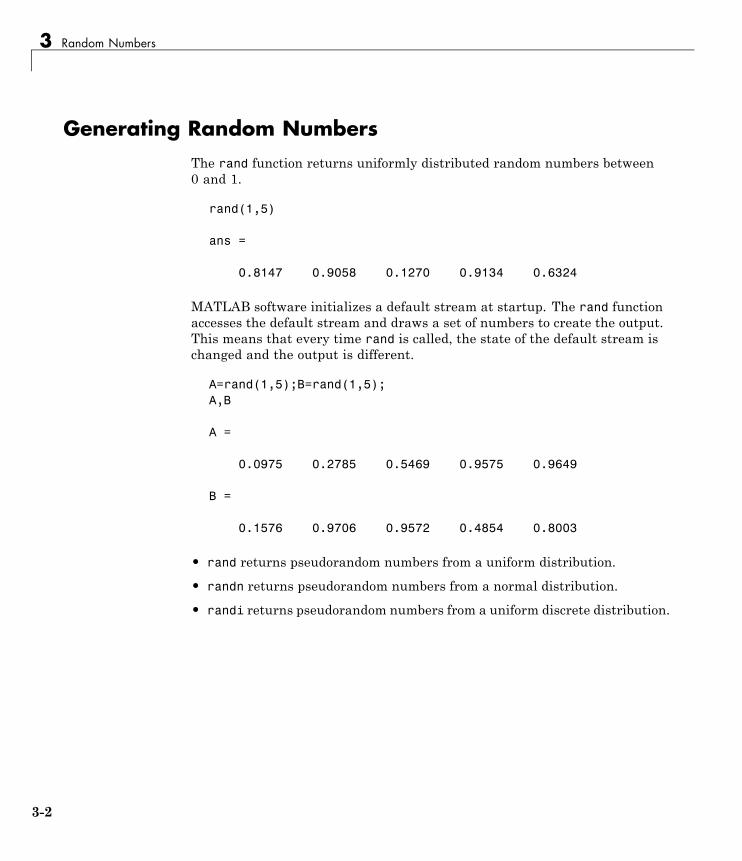
3 Random Numbers
Generating Random NumbersThe rand function returns uniformly distributed random numbers between0 and 1.
rand(1,5)
ans =
0.8147 0.9058 0.1270 0.9134 0.6324
MATLAB software initializes a default stream at startup. The rand functionaccesses the default stream and draws a set of numbers to create the output.This means that every time rand is called, the state of the default stream ischanged and the output is different.
A=rand(1,5);B=rand(1,5);A,B
A =
0.0975 0.2785 0.5469 0.9575 0.9649
B =
0.1576 0.9706 0.9572 0.4854 0.8003
• rand returns pseudorandom numbers from a uniform distribution.
• randn returns pseudorandom numbers from a normal distribution.
• randi returns pseudorandom numbers from a uniform discrete distribution.
3-2

Managing the Default Stream
Managing the Default Streamrand, randn, and randi draw random numbers from an underlying randomnumber stream, called the default stream. The @RandStream class allows youto get a handle to the default stream and control random number generation.
Get a handle to the default stream as follows:
defaultStream=RandStream.getDefaultStream
defaultStream =
mt19937ar random stream (current default)Seed: 0
RandnAlg: Ziggurat
Return the properties of the stream object with the get method:
get(defaultStream)Type: 'mt19937ar'
NumStreams: 1StreamIndex: 1
Substream: 1Seed: 0
State: [625x1 uint32]RandnAlg: 'Ziggurat'
Antithetic: 0FullPrecision: 1
Now, use the rand function to generate uniform random values from thedefault stream.
rand(1,5);
Use the randn and randi functions to generate normal random values andinteger random values from the default stream.
A=randi(100,1,5);A=randn(1,5);
3-3
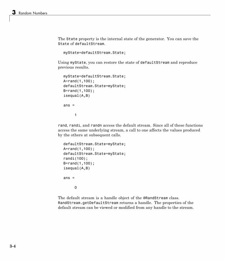
3 Random Numbers
The State property is the internal state of the generator. You can save theState of defaultStream.
myState=defaultStream.State;
Using myState, you can restore the state of defaultStream and reproduceprevious results.
myState=defaultStream.State;A=rand(1,100);defaultStream.State=myState;B=rand(1,100);isequal(A,B)
ans =
1
rand, randi, and randn access the default stream. Since all of these functionsaccess the same underlying stream, a call to one affects the values producedby the others at subsequent calls.
defaultStream.State=myState;A=rand(1,100);defaultStream.State=myState;randi(100);B=rand(1,100);isequal(A,B)
ans =
0
The default stream is a handle object of the @RandStream class.RandStream.getDefaultStream returns a handle. The properties of thedefault stream can be viewed or modified from any handle to the stream.
3-4
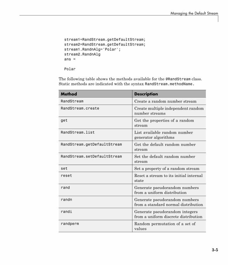
Managing the Default Stream
stream1=RandStream.getDefaultStream;stream2=RandStream.getDefaultStream;stream1.RandnAlg='Polar';stream2.RandnAlgans =
Polar
The following table shows the methods available for the @RandStream class.Static methods are indicated with the syntax RandStream.methodName.
Method Description
RandStream Create a random number stream
RandStream.create Create multiple independent randomnumber streams
get Get the properties of a randomstream
RandStream.list List available random numbergenerator algorithms
RandStream.getDefaultStream Get the default random numberstream
RandStream.setDefaultStream Set the default random numberstream
set Set a property of a random stream
reset Reset a stream to its initial internalstate
rand Generate pseudorandom numbersfrom a uniform distribution
randn Generate pseudorandom numbersfrom a standard normal distribution
randi Generate pseudorandom integersfrom a uniform discrete distribution
randperm Random permutation of a set ofvalues
3-5
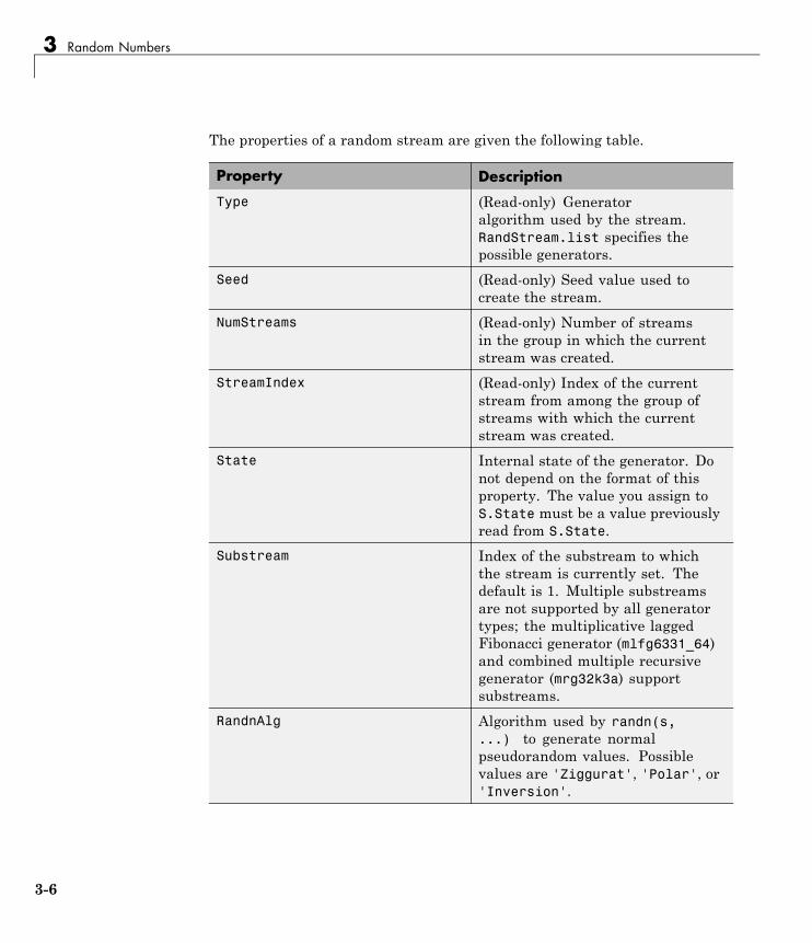
3 Random Numbers
The properties of a random stream are given the following table.
Property Description
Type (Read-only) Generatoralgorithm used by the stream.RandStream.list specifies thepossible generators.
Seed (Read-only) Seed value used tocreate the stream.
NumStreams (Read-only) Number of streamsin the group in which the currentstream was created.
StreamIndex (Read-only) Index of the currentstream from among the group ofstreams with which the currentstream was created.
State Internal state of the generator. Donot depend on the format of thisproperty. The value you assign toS.State must be a value previouslyread from S.State.
Substream Index of the substream to whichthe stream is currently set. Thedefault is 1. Multiple substreamsare not supported by all generatortypes; the multiplicative laggedFibonacci generator (mlfg6331_64)and combined multiple recursivegenerator (mrg32k3a) supportsubstreams.
RandnAlg Algorithm used by randn(s,...) to generate normalpseudorandom values. Possiblevalues are 'Ziggurat', 'Polar', or'Inversion'.
3-6
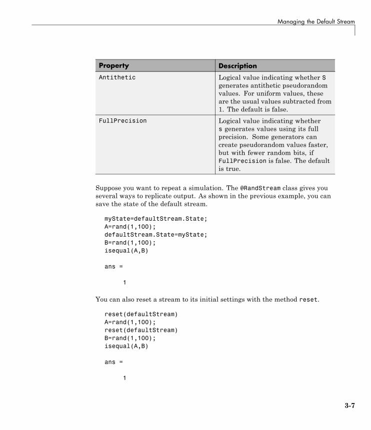
Managing the Default Stream
Property Description
Antithetic Logical value indicating whether Sgenerates antithetic pseudorandomvalues. For uniform values, theseare the usual values subtracted from1. The default is false.
FullPrecision Logical value indicating whethers generates values using its fullprecision. Some generators cancreate pseudorandom values faster,but with fewer random bits, ifFullPrecision is false. The defaultis true.
Suppose you want to repeat a simulation. The @RandStream class gives youseveral ways to replicate output. As shown in the previous example, you cansave the state of the default stream.
myState=defaultStream.State;A=rand(1,100);defaultStream.State=myState;B=rand(1,100);isequal(A,B)
ans =
1
You can also reset a stream to its initial settings with the method reset.
reset(defaultStream)A=rand(1,100);reset(defaultStream)B=rand(1,100);isequal(A,B)
ans =
1
3-7
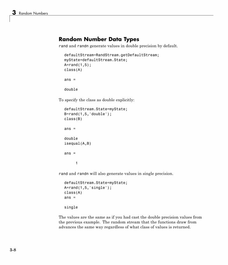
3 Random Numbers
Random Number Data Typesrand and randn generate values in double precision by default.
defaultStream=RandStream.getDefaultStream;myState=defaultStream.State;A=rand(1,5);class(A)
ans =
double
To specify the class as double explicitly:
defaultStream.State=myState;B=rand(1,5,'double');class(B)
ans =
doubleisequal(A,B)
ans =
1
rand and randn will also generate values in single precision.
defaultStream.State=myState;A=rand(1,5,'single');class(A)ans =
single
The values are the same as if you had cast the double precision values fromthe previous example. The random stream that the functions draw fromadvances the same way regardless of what class of values is returned.
3-8
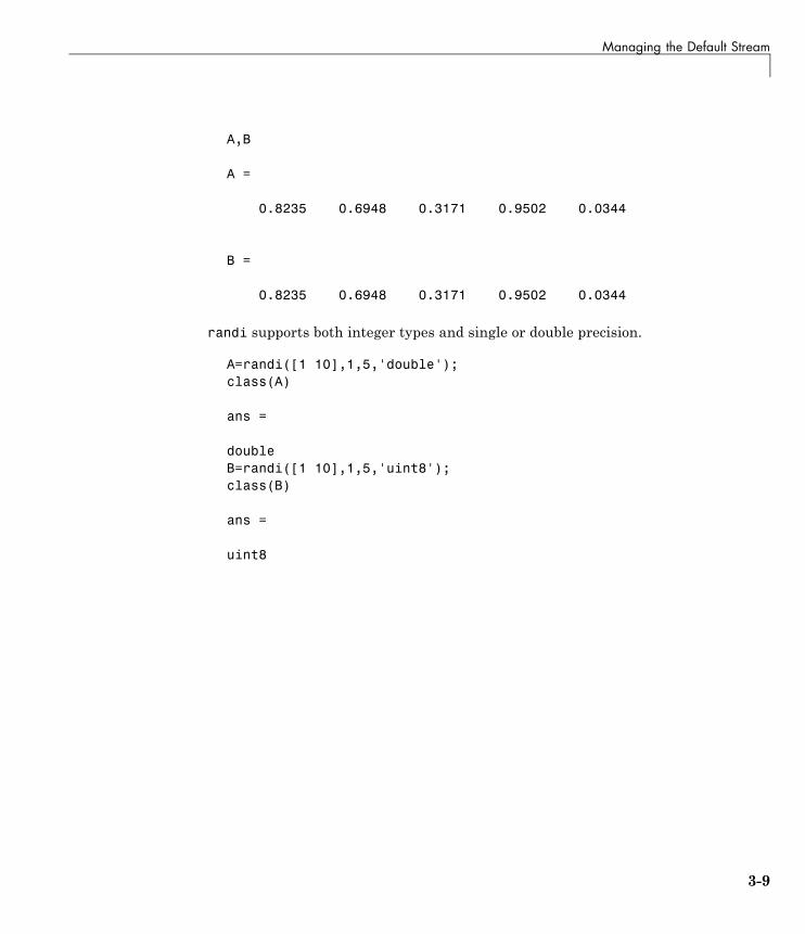
Managing the Default Stream
A,B
A =
0.8235 0.6948 0.3171 0.9502 0.0344
B =
0.8235 0.6948 0.3171 0.9502 0.0344
randi supports both integer types and single or double precision.
A=randi([1 10],1,5,'double');class(A)
ans =
doubleB=randi([1 10],1,5,'uint8');class(B)
ans =
uint8
3-9
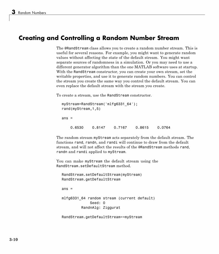
3 Random Numbers
Creating and Controlling a Random Number StreamThe @RandStream class allows you to create a random number stream. This isuseful for several reasons. For example, you might want to generate randomvalues without affecting the state of the default stream. You might wantseparate sources of randomness in a simulation. Or you may need to use adifferent generator algorithm than the one MATLAB software uses at startup.With the RandStream constructor, you can create your own stream, set thewritable properties, and use it to generate random numbers. You can controlthe stream you create the same way you control the default stream. You caneven replace the default stream with the stream you create.
To create a stream, use the RandStream constructor.
myStream=RandStream('mlfg6331_64');rand(myStream,1,5)
ans =
0.6530 0.8147 0.7167 0.8615 0.0764
The random stream myStream acts separately from the default stream. Thefunctions rand, randn, and randi will continue to draw from the defaultstream, and will not affect the results of the @RandStream methods rand,randn and randi applied to myStream.
You can make myStream the default stream using theRandStream.setDefaultStream method.
RandStream.setDefaultStream(myStream)RandStream.getDefaultStream
ans =
mlfg6331_64 random stream (current default)Seed: 0
RandnAlg: Ziggurat
RandStream.getDefaultStream==myStream
3-10
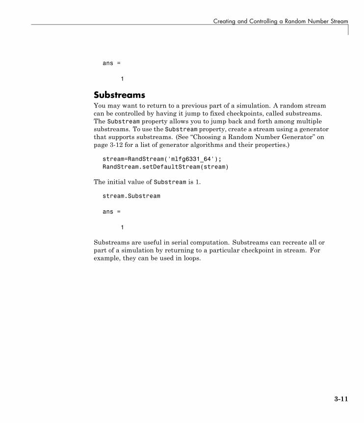
Creating and Controlling a Random Number Stream
ans =
1
SubstreamsYou may want to return to a previous part of a simulation. A random streamcan be controlled by having it jump to fixed checkpoints, called substreams.The Substream property allows you to jump back and forth among multiplesubstreams. To use the Substream property, create a stream using a generatorthat supports substreams. (See “Choosing a Random Number Generator” onpage 3-12 for a list of generator algorithms and their properties.)
stream=RandStream('mlfg6331_64');RandStream.setDefaultStream(stream)
The initial value of Substream is 1.
stream.Substream
ans =
1
Substreams are useful in serial computation. Substreams can recreate all orpart of a simulation by returning to a particular checkpoint in stream. Forexample, they can be used in loops.
3-11
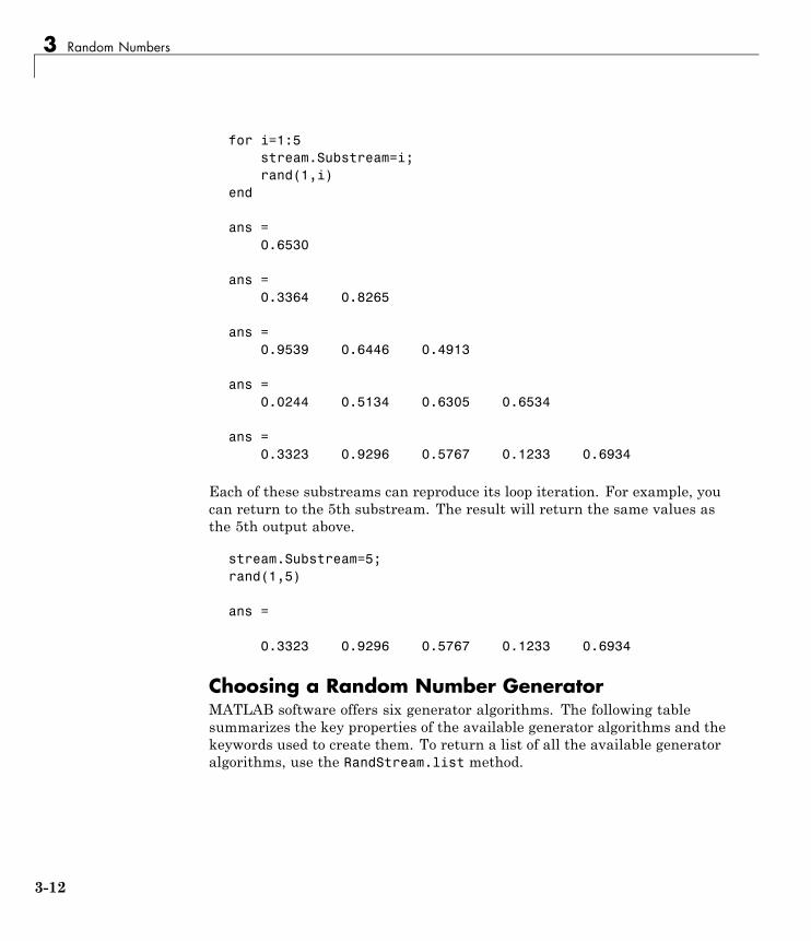
3 Random Numbers
for i=1:5stream.Substream=i;rand(1,i)
end
ans =0.6530
ans =0.3364 0.8265
ans =0.9539 0.6446 0.4913
ans =0.0244 0.5134 0.6305 0.6534
ans =0.3323 0.9296 0.5767 0.1233 0.6934
Each of these substreams can reproduce its loop iteration. For example, youcan return to the 5th substream. The result will return the same values asthe 5th output above.
stream.Substream=5;rand(1,5)
ans =
0.3323 0.9296 0.5767 0.1233 0.6934
Choosing a Random Number GeneratorMATLAB software offers six generator algorithms. The following tablesummarizes the key properties of the available generator algorithms and thekeywords used to create them. To return a list of all the available generatoralgorithms, use the RandStream.list method.
3-12
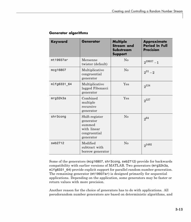
Creating and Controlling a Random Number Stream
Generator algorithms
Keyword Generator MultipleStream andSubstreamSupport
ApproximatePeriod In FullPrecision
mt19937ar Mersennetwister (default)
No2 119937 −
mcg16807 Multiplicativecongruentialgenerator
No2 231 −
mlfg6331_64 Multiplicativelagged Fibonaccigenerator
Yes2124
mrg32k3a Combinedmultiplerecursivegenerator
Yes2127
shr3cong Shift-registergeneratorsummedwith linearcongruentialgenerator
No264
swb2712 Modifiedsubtract withborrow generator
No21492
Some of the generators (mcg16807, shr3cong, swb2712) provide for backwardscompatibility with earlier versions of MATLAB. Two generators (mrg32k3a,mlfg6331_64) provide explicit support for parallel random number generation.The remaining generator (mt19937ar) is designed primarily for sequentialapplications. Depending on the application, some generators may be faster orreturn values with more precision.
Another reason for the choice of generators has to do with applications. Allpseudorandom number generators are based on deterministic algorithms, and
3-13

3 Random Numbers
all will fail a sufficiently specific statistical test for randomness. One way tocheck the results of a Monte Carlo simulation is to rerun the simulation withtwo or more different generator algorithms, and MATLAB software’s choiceof generators provide you with the means to do that. Although it is unlikelythat your results will differ by more than Monte Carlo sampling error whenusing different generators, there are examples in the literature where thiskind of validation has turned up flaws in a particular generator algorithm(see [10] for an example).
Generator Algorithms
mcg16807A 32-bit multiplicative congruential generator, as described in [11],
with multiplier a = 75 , modulo m = −2 131 . This generator has a period
of 2 231 − and does not support multiple streams or substreams. EachU(0,1) value is created using a single 32-bit integer from the generator;
the possible values are all multiples of ( )2 131 1− − strictly within theinterval (0,1). The randn algorithm used by default for mcg16807streams is the polar algorithm (described in [1]). Note: This generatoris identical to the one used beginning in MATLAB Version 4 by boththe rand and randn functions, activated using rand('seed',s) orrandn('seed',s).
mlfg6331_64A 64-bit multiplicative lagged Fibonacci generator, as described in
[8], with lags l = 63 , k = 31 . This generator is similar to the MLFGimplemented in the SPRNG package. It has a period of approximately
2124 . It supports up to 261 parallel streams, via parameterization,
and 251 substreams each of length 272 . Each U(0,1) value is createdusing one 64-bit integer from the generator; the possible values are all
multiples of 2 53− strictly within the interval (0,1). The randn algorithmused by default for mlfg6331_64 streams is the ziggurat algorithm [5],but with the mlfg6331_64 generator underneath.
mrg32k3aA 32-bit combined multiple recursive generator, as described in [3].This generator is similar to the CMRG implemented in the RngStreams
3-14
Creating and Controlling a Random Number Stream
package. It has a period of 2127 , and supports up to 263 parallel
streams, via sequence splitting, and 251 substreams each of length
276 . Each U(0,1) value is created using two 32-bit integers from the
generator; the possible values are multiples of 2 53− strictly withinthe interval (0,1). The randn algorithm used by default for mrg32k3astreams is the ziggurat algorithm [5], but with the mrg32k3a generatorunderneath.
mt19937arThe Mersenne Twister, as described in [9], with Mersenne
prime 2 119937 − . This is the generator documented athttp://www.math.sci.hiroshima-u.ac.jp/~m-mat/MT/emt.html. It
has a period of 2 119937 − . Each U(0,1) value is created using two 32-bitintegers from the generator; the possible values are all multiples of
2 53− strictly within the interval (0,1). This generator does not supportmultiple streams or substreams. The randn algorithm used by defaultfor mt19937ar streams is the ziggurat algorithm [5], but with themt19937ar generator underneath. Note: This generator is identical tothe one used by the rand function beginning in MATLAB Version 7,activated using rand('twister',s).
shr3congMarsaglia’s SHR3 shift-register generator summed with a linear
congruential generator with multiplier a = 69069 , addend b = 1234567 ,
and modulus 2 32− . SHR3 is a 3-shift-register generator defined as
u u= + + +( )( )( )I L I R I L17 13 5 , where I is the identity operator, L isthe left shift operator, and R is the right shift operator. The combined
generator (described in [4]) has a period of approximately 264 . Thisgenerator does not support multiple streams or substreams. EachU(0,1) value is created using one 32-bit integer from the generator; the
possible values are all multiples of 2 32− strictly within the interval(0,1). The randn algorithm used by default for shr3cong streams isthe earlier form of the ziggurat algorithm [7], but with the shr3conggenerator underneath. Note: This generator is identical to the one usedby the randn function beginning in MATLAB Version 5, activated usingrandn('state',s).
3-15
3 Random Numbers
swb2712A modified Subtract-with-Borrow generator, as described in [6]. Thisgenerator is similar to an additive lagged Fibonacci generator with lags27 and 12, but is modified to have a much longer period of approximately
21492 . The generator works natively in double precision to create U(0,1)values, and all values in the open interval (0,1) are possible. The randnalgorithm used by default for swb2712 streams is the ziggurat algorithm[5], but with the swb2712 generator underneath. Note: This generatoris identical to the one used by the rand function beginning in MATLABVersion 5, activated using rand('state',s).
Transformation Algorithms
InversionComputes a normal random variate by applying the standard normalinverse cumulative distribution function to a uniform random variate.Exactly one uniform value is consumed per normal value.
PolarThe polar rejection algorithm, as described in [1]. Approximately 1.27uniform values are consumed per normal value, on average.
ZigguratThe ziggurat algorithm, as described in [5]. Approximately 2.02 uniformvalues are consumed per normal value, on average.
Compatibility ConsiderationsIn MATLAB versions 7.6 and prior, the way to replicate results involvingrandom numbers was to use keyword and seed value arguments with the randand randn functions.
3-16
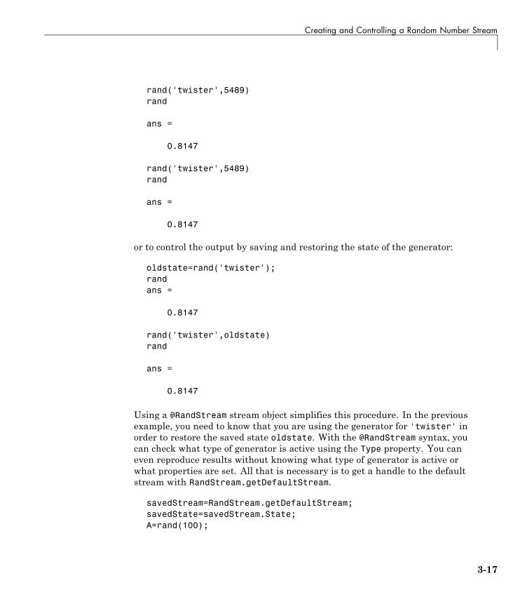
Creating and Controlling a Random Number Stream
rand('twister',5489)rand
ans =
0.8147
rand('twister',5489)rand
ans =
0.8147
or to control the output by saving and restoring the state of the generator:
oldstate=rand('twister');randans =
0.8147
rand('twister',oldstate)rand
ans =
0.8147
Using a @RandStream stream object simplifies this procedure. In the previousexample, you need to know that you are using the generator for 'twister' inorder to restore the saved state oldstate. With the @RandStream syntax, youcan check what type of generator is active using the Type property. You caneven reproduce results without knowing what type of generator is active orwhat properties are set. All that is necessary is to get a handle to the defaultstream with RandStream.getDefaultStream.
savedStream=RandStream.getDefaultStream;savedState=savedStream.State;A=rand(100);
3-17
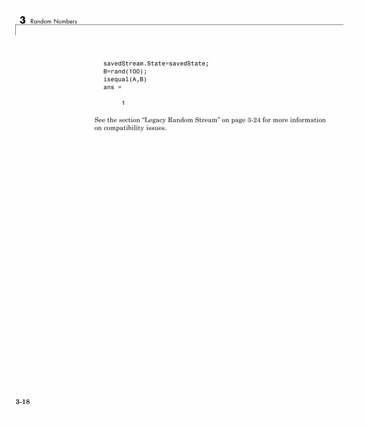
3 Random Numbers
savedStream.State=savedState;B=rand(100);isequal(A,B)ans =
1
See the section “Legacy Random Stream” on page 3-24 for more informationon compatibility issues.
3-18
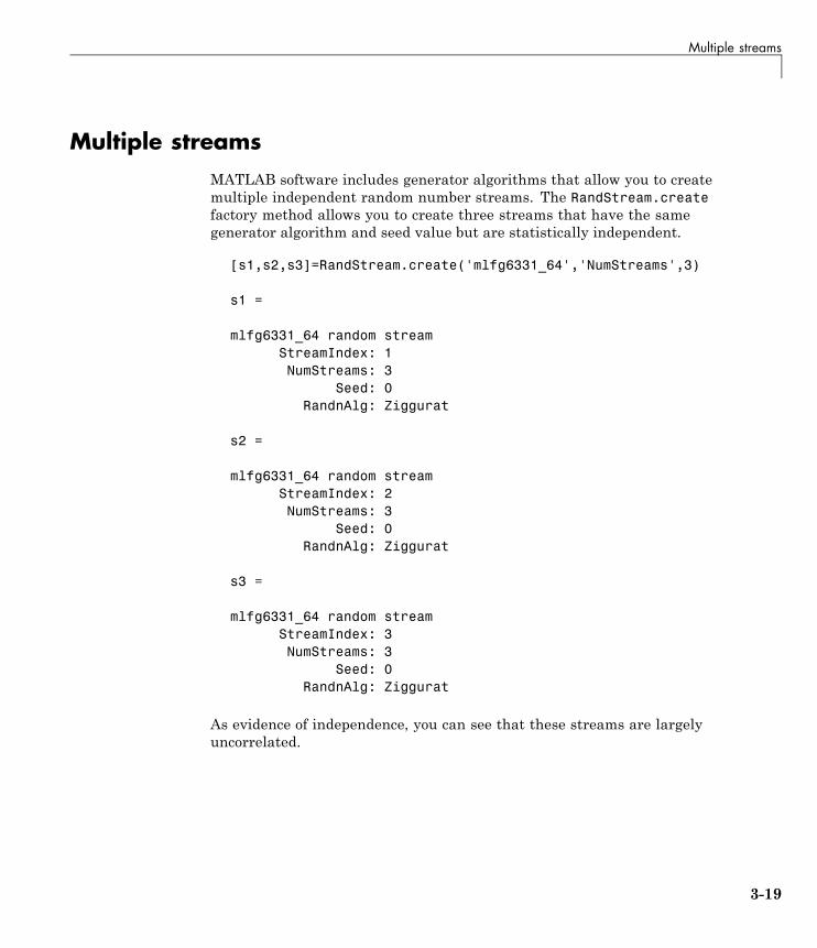
Multiple streams
Multiple streamsMATLAB software includes generator algorithms that allow you to createmultiple independent random number streams. The RandStream.createfactory method allows you to create three streams that have the samegenerator algorithm and seed value but are statistically independent.
[s1,s2,s3]=RandStream.create('mlfg6331_64','NumStreams',3)
s1 =
mlfg6331_64 random streamStreamIndex: 1NumStreams: 3
Seed: 0RandnAlg: Ziggurat
s2 =
mlfg6331_64 random streamStreamIndex: 2NumStreams: 3
Seed: 0RandnAlg: Ziggurat
s3 =
mlfg6331_64 random streamStreamIndex: 3NumStreams: 3
Seed: 0RandnAlg: Ziggurat
As evidence of independence, you can see that these streams are largelyuncorrelated.
3-19
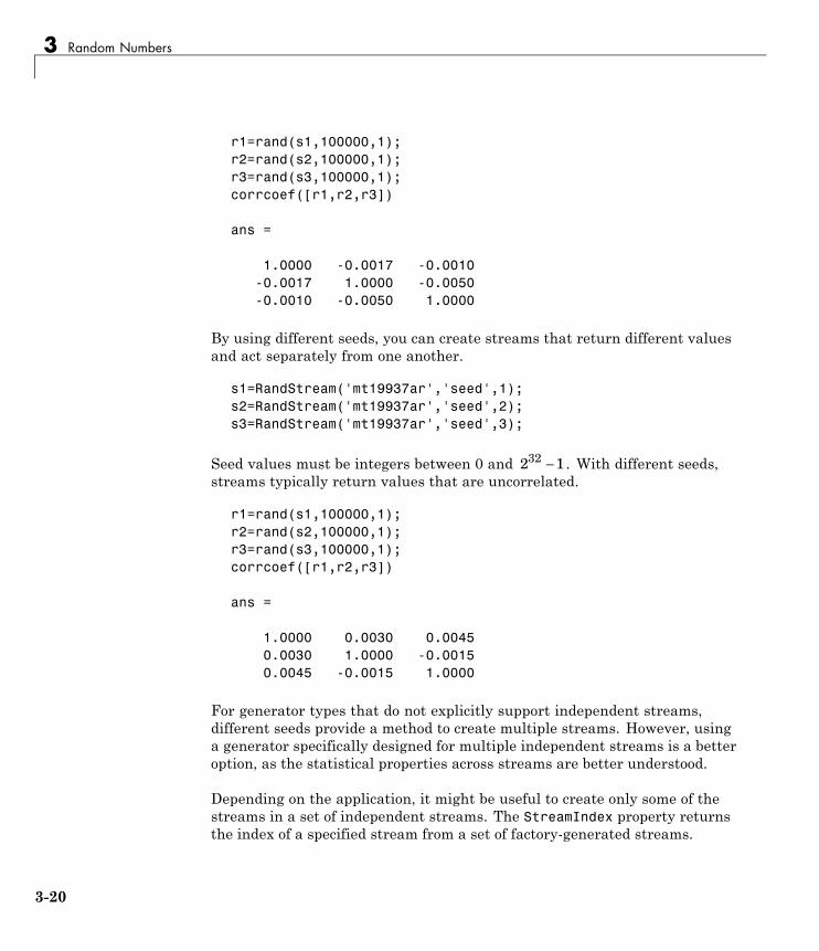
3 Random Numbers
r1=rand(s1,100000,1);r2=rand(s2,100000,1);r3=rand(s3,100000,1);corrcoef([r1,r2,r3])
ans =
1.0000 -0.0017 -0.0010-0.0017 1.0000 -0.0050-0.0010 -0.0050 1.0000
By using different seeds, you can create streams that return different valuesand act separately from one another.
s1=RandStream('mt19937ar','seed',1);s2=RandStream('mt19937ar','seed',2);s3=RandStream('mt19937ar','seed',3);
Seed values must be integers between 0 and 2 132 − . With different seeds,streams typically return values that are uncorrelated.
r1=rand(s1,100000,1);r2=rand(s2,100000,1);r3=rand(s3,100000,1);corrcoef([r1,r2,r3])
ans =
1.0000 0.0030 0.00450.0030 1.0000 -0.00150.0045 -0.0015 1.0000
For generator types that do not explicitly support independent streams,different seeds provide a method to create multiple streams. However, usinga generator specifically designed for multiple independent streams is a betteroption, as the statistical properties across streams are better understood.
Depending on the application, it might be useful to create only some of thestreams in a set of independent streams. The StreamIndex property returnsthe index of a specified stream from a set of factory-generated streams.
3-20

Multiple streams
numLabs=256;labIndex=4;s1=RandStream.create('mlfg6331_64',
'NumStreams',numLabs,'StreamIndices',labIndex)
s1=mlfg6331_64 random stream
StreamIndex: 4NumStreams: 256
Seed: 0RandnAlg: Ziggurat
Multiple streams, since they are statistically independent, can be usedto verify the precision of a simulation. For example, a set of independentstreams can be used to repeat a Monte Carlo simulation several times indifferent MATLAB sessions or on different processors and determine thevariance in the results. This makes multiple streams useful in large-scaleparallel simulations.
Note Not all generators algorithms support multiple streams. See the tableof generator algorithms in “Choosing a Random Number Generator” on page3-12 for a summary of generator properties.
3-21
3 Random Numbers
Updating Your Random Number Generator SyntaxBefore MATLAB Version 7.7 (R2008b), the rand and randn functions used adifferent syntax for controlling the random number generators. In addition,rand and randn had separate underlying random number streams.
For example, in MATLAB Version 7.5 (R2007b), the syntax to reset the randfunction to its startup setting in MATLAB was:
rand('twister',5489)
The syntax to reset the randn function to its startup setting in MATLAB was:
randn('state',0)
Note The syntaxes rand('keyword',seed_value) andrandn('keyword',seed_value) are still supported in the currentversion of MATLAB, though they are not recommended.
The old control syntaxes for rand and randn do two things:
• The first argument—the keyword—selected a random number generator.
• The second argument specified an integer seed or a state vector with whichto reinitialize that generator.
For example, the 'state' keyword in rand('state',0) did not initialize thestate of whatever generator was currently active, but rather activated theMATLAB Version 5 generator and initialized it with the seed 0. Similarly,the 'seed' keyword in rand('seed',0) did not set the seed of whatevergenerator was currently active, but rather activated the MATLAB Version 4generator and initialized it with the seed 0.
In the new RandStream syntax, the first argument to RandStream selects thegenerator type. The other arguments are name-value pairs that allow you toset a seed value and choose a transformation algorithm for randn. To updateyour code so that you get the same sequences of random numbers as in yourold code, use the following tables:
3-22
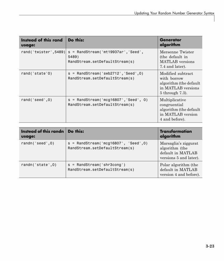
Updating Your Random Number Generator Syntax
Instead of this randusage:
Do this: Generatoralgorithm
rand('twister',5489) s = RandStream('mt19937ar','Seed',5489)RandStream.setDefaultStream(s)
Mersenne Twister(the default inMATLAB versions7.4 and later).
rand('state'0) s = RandStream('swb2712','Seed',0)RandStream.setDefaultStream(s)
Modified subtractwith borrowalgorithm (the defaultin MATLAB versions5 through 7.3).
rand('seed',0) s = RandStream('mcg16807','Seed', 0)RandStream.setDefaultStream(s)
Multiplicativecongruentialalgorithm (the defaultin MATLAB version4 and before).
Instead of this randnusage:
Do this: Transformationalgorithm
randn('seed',0) s = RandStream('mcg16807', 'Seed',0)RandStream.setDefaultStream(s)
Marsaglia’s zigguratalgorithm (thedefault in MATLABversions 5 and later).
randn('state',0) s = RandStream('shr3cong')RandStream.setDefaultStream(s)
Polar algorithm (thedefault in MATLABversion 4 and before).
3-23
3 Random Numbers
Tip In MATLAB V7.6 (R2008a) and above, the functions rand and randndraw from the same random number stream and apply a transformationto produce the desired distribution. When using the the legacy randomstream, however, rand and randn have completely separate streams. UsingRandStream, there is no simple way to replicate the exact number sequencescreated by running this sequence of commands, for example:
rand('state',0)randn(`state',0)rand( )randn( )
You should use the legacy random stream to replicate such sequences.
Legacy Random StreamAny use of the syntax rand('keyword', value), where value is an integerwill activate the legacy random stream.
rand('twister',5489)RandStream.getDefaultStream
ans =
legacy random stream (current default)RAND algorithm: V7.4 (Mersenne Twister)
RANDN algorithm: V5 (Ziggurat)
While the legacy random stream is active, rand and randn use separategenerators. The generator used for each function is determined by thekeyword argument of the function. For example, the twister keyword willactivate the Mersenne Twister generator for rand and the ziggurat algorithmfor randn. While the legacy random stream is active, you can use the oldcontrol syntax to activate other legacy generators as well. The old controlsyntaxes for rand and randn and their equivalents with the RandStreamconstructor are given in the tables above. (The randi function is new inMATLAB Version 7.7 (R2008b) and does not accept legacy random streamkeyword arguments. It can be used with the legacy random stream; in whichcase it uses the same generator as rand.)
3-24
Updating Your Random Number Generator Syntax
While the legacy random stream is active, you may still create random streamobjects and generate values from those streams using RandStream methods.All of the generator and transformation algorithms that were available inMATLAB Version 7.6 (R2008a) and earlier are available in the currentversion.
Deactivating the Legacy Random StreamUse of an old syntax (rand('keyword',value), randn('keyword',value))will will activate the legacy random stream. To deactivate the legacy randomstream, create a new random stream with the RandStream constructor andmake it the default stream.
1 Create a number stream:
s = RandStream('mt19937ar')
2 Make it the default stream:
RandStream.setDefaultStream(s)
3-25

3 Random Numbers
Selected Bibliography[1] Devroye, L. Non-Uniform Random VariateGeneration, Springer-Verlag, 1986. Available online athttp://cg.scs.carleton.ca/~luc/rnbookindex.html.
[2] L’Ecuyer, P. and R. Simard. “TestU01: A C Library for Empirical Testingof Random Number Generators,” ACM Transactions on MathematicalSoftware, 33(4): Article 22. 2007.
[3] L’Ecuyer, P., R. Simard, E. J. Chen, and W. D. Kelton. “AnObjected-Oriented Random-Number Package with Many Long Streams andSubstreams.” Operations Research, 50(6):1073–1075. 2002.
[4] Marsaglia, G. “Random numbers for C: The END?”Usenet posting to sci.stat.math. 1999. Available online athttp://groups.google.com/group/sci.crypt/browse_thread/thread/ca8682a4658a124d/.
[5] Marsaglia G., and W. W. Tsang. “The ziggurat method for generatingrandom variables.” Journal of Statistical Software, 5:1–7. 2000. Availableonline at http://www.jstatsoft.org/v05/i08.
[6] Marsaglia, G., and A. Zaman. “A new class of random number generators.”Annals of Applied Probability 1(3):462–480. 1991.
[7] Marsaglia, G., and W. W. Tsang. “A fast, easily implemented method forsampling from decreasing or symmetric unimodal density functions.” SIAMJ.Sci.Stat.Comput. 5(2):349–359. 1984.
[8] Mascagni, M., and A. Srinivasan. “Parameterizing Parallel MultiplicativeLagged-Fibonacci Generators.” Parallel Computing, 30: 899–916. 2004.
[9] Matsumoto, M., and T. Nishimura.“Mersenne Twister: A623-Dimensionally Equidistributed Uniform Pseudorandom NumberGenerator.” ACM Transactions on Modeling and Computer Simulation,8(1):3–30. 1998.
[10] Moler, C.B. Numerical Computing with MATLAB. SIAM, 2004. Availableonline at http://www.mathworks.com/moler
3-26

Selected Bibliography
[11] Park, S.K., and K.W. Miller. “Random Number Generators: Good OnesAre Hard to Find.” Communications of the ACM, 31(10):1192–1201. 1998.
3-27

3 Random Numbers
3-28

4
Sparse Matrices
• “Function Summary” on page 4-2
• “Computational Advantages” on page 4-10
• “Constructing Sparse Matrices” on page 4-13
• “Accessing Sparse Matrices” on page 4-19
• “Sparse Matrix Operations” on page 4-25
• “Selected Bibliography” on page 4-45
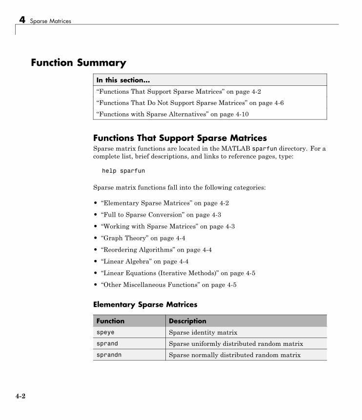
4 Sparse Matrices
Function Summary
In this section...
“Functions That Support Sparse Matrices” on page 4-2
“Functions That Do Not Support Sparse Matrices” on page 4-6
“Functions with Sparse Alternatives” on page 4-10
Functions That Support Sparse MatricesSparse matrix functions are located in the MATLAB sparfun directory. For acomplete list, brief descriptions, and links to reference pages, type:
help sparfun
Sparse matrix functions fall into the following categories:
• “Elementary Sparse Matrices” on page 4-2
• “Full to Sparse Conversion” on page 4-3
• “Working with Sparse Matrices” on page 4-3
• “Graph Theory” on page 4-4
• “Reordering Algorithms” on page 4-4
• “Linear Algebra” on page 4-4
• “Linear Equations (Iterative Methods)” on page 4-5
• “Other Miscellaneous Functions” on page 4-5
Elementary Sparse Matrices
Function Description
speye Sparse identity matrix
sprand Sparse uniformly distributed random matrix
sprandn Sparse normally distributed random matrix
4-2
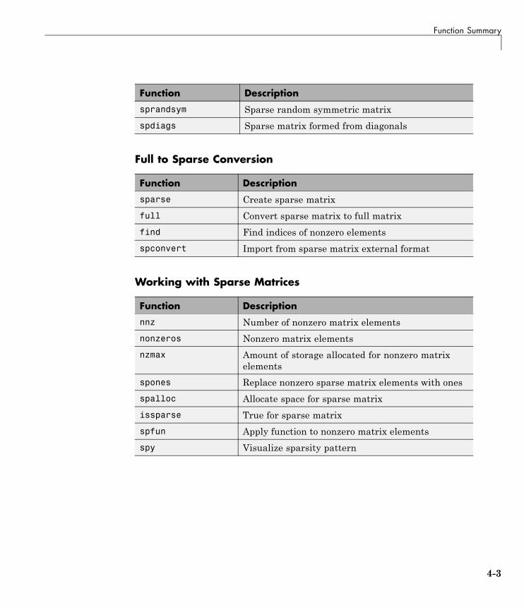
Function Summary
Function Description
sprandsym Sparse random symmetric matrix
spdiags Sparse matrix formed from diagonals
Full to Sparse Conversion
Function Description
sparse Create sparse matrix
full Convert sparse matrix to full matrix
find Find indices of nonzero elements
spconvert Import from sparse matrix external format
Working with Sparse Matrices
Function Description
nnz Number of nonzero matrix elements
nonzeros Nonzero matrix elements
nzmax Amount of storage allocated for nonzero matrixelements
spones Replace nonzero sparse matrix elements with ones
spalloc Allocate space for sparse matrix
issparse True for sparse matrix
spfun Apply function to nonzero matrix elements
spy Visualize sparsity pattern
4-3
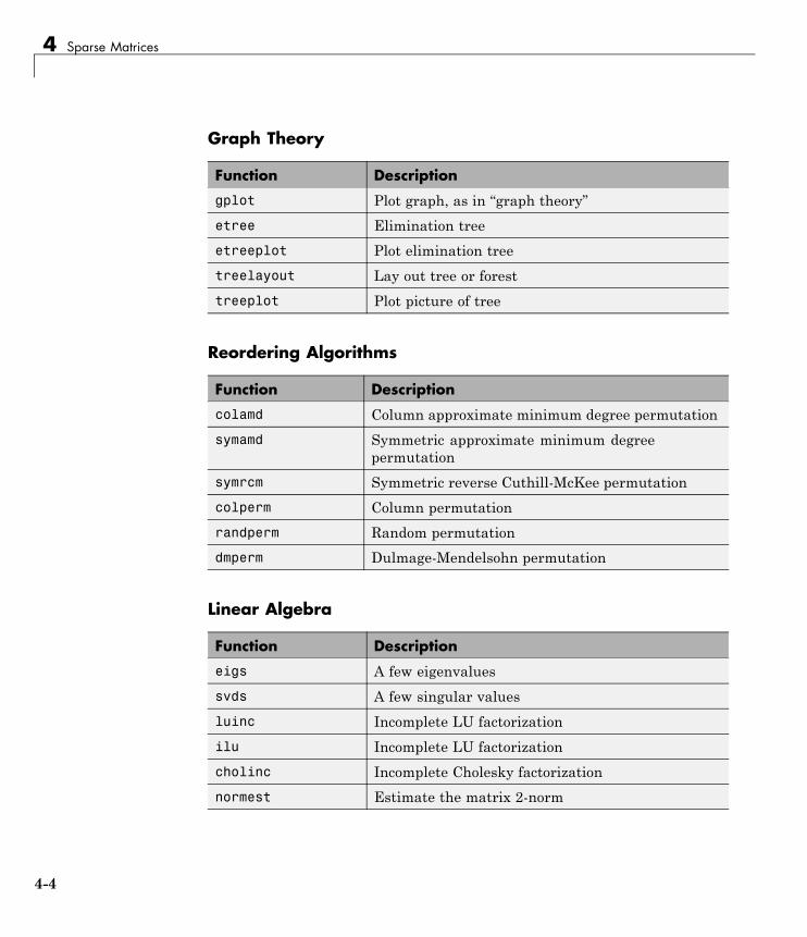
4 Sparse Matrices
Graph Theory
Function Description
gplot Plot graph, as in “graph theory”
etree Elimination tree
etreeplot Plot elimination tree
treelayout Lay out tree or forest
treeplot Plot picture of tree
Reordering Algorithms
Function Description
colamd Column approximate minimum degree permutation
symamd Symmetric approximate minimum degreepermutation
symrcm Symmetric reverse Cuthill-McKee permutation
colperm Column permutation
randperm Random permutation
dmperm Dulmage-Mendelsohn permutation
Linear Algebra
Function Description
eigs A few eigenvalues
svds A few singular values
luinc Incomplete LU factorization
ilu Incomplete LU factorization
cholinc Incomplete Cholesky factorization
normest Estimate the matrix 2-norm
4-4
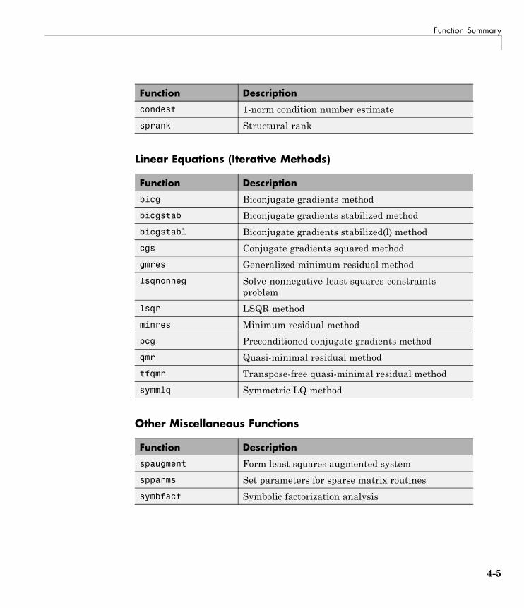
Function Summary
Function Description
condest 1-norm condition number estimate
sprank Structural rank
Linear Equations (Iterative Methods)
Function Description
bicg Biconjugate gradients method
bicgstab Biconjugate gradients stabilized method
bicgstabl Biconjugate gradients stabilized(l) method
cgs Conjugate gradients squared method
gmres Generalized minimum residual method
lsqnonneg Solve nonnegative least-squares constraintsproblem
lsqr LSQR method
minres Minimum residual method
pcg Preconditioned conjugate gradients method
qmr Quasi-minimal residual method
tfqmr Transpose-free quasi-minimal residual method
symmlq Symmetric LQ method
Other Miscellaneous Functions
Function Description
spaugment Form least squares augmented system
spparms Set parameters for sparse matrix routines
symbfact Symbolic factorization analysis
4-5
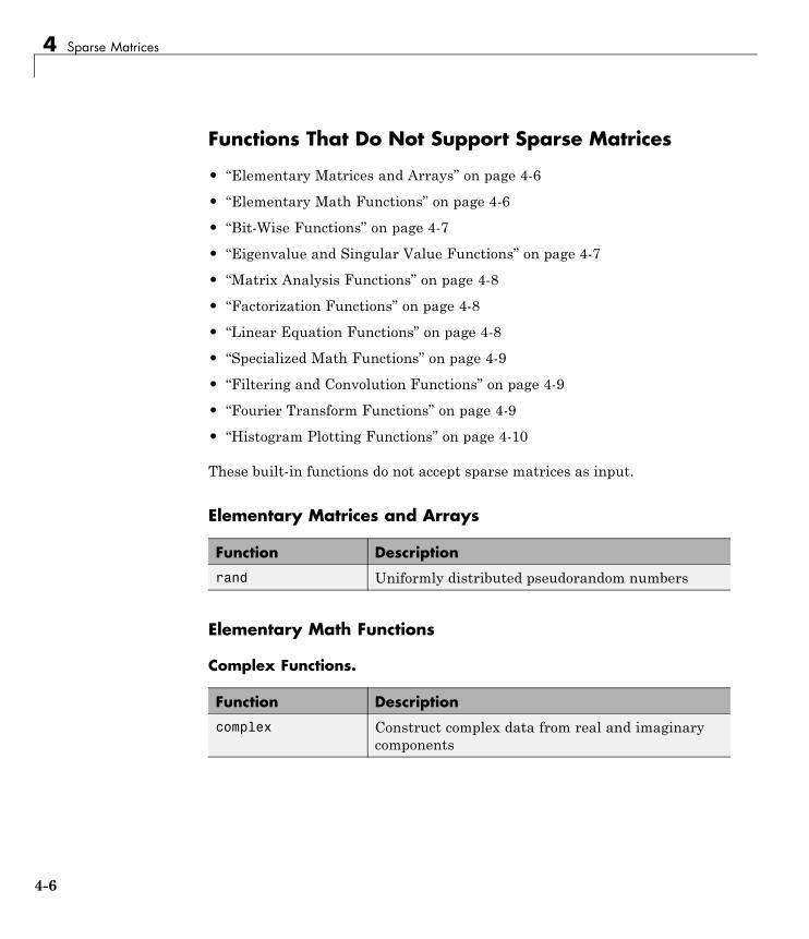
4 Sparse Matrices
Functions That Do Not Support Sparse Matrices
• “Elementary Matrices and Arrays” on page 4-6
• “Elementary Math Functions” on page 4-6
• “Bit-Wise Functions” on page 4-7
• “Eigenvalue and Singular Value Functions” on page 4-7
• “Matrix Analysis Functions” on page 4-8
• “Factorization Functions” on page 4-8
• “Linear Equation Functions” on page 4-8
• “Specialized Math Functions” on page 4-9
• “Filtering and Convolution Functions” on page 4-9
• “Fourier Transform Functions” on page 4-9
• “Histogram Plotting Functions” on page 4-10
These built-in functions do not accept sparse matrices as input.
Elementary Matrices and Arrays
Function Description
rand Uniformly distributed pseudorandom numbers
Elementary Math Functions
Complex Functions.
Function Description
complex Construct complex data from real and imaginarycomponents
4-6
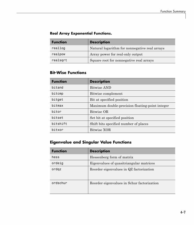
Function Summary
Real Array Exponential Functions.
Function Description
reallog Natural logarithm for nonnegative real arrays
realpow Array power for real-only output
realsqrt Square root for nonnegative real arrays
Bit-Wise Functions
Function Description
bitand Bitwise AND
bitcmp Bitwise complement
bitget Bit at specified position
bitmax Maximum double-precision floating-point integer
bitor Bitwise OR
bitset Set bit at specified position
bitshift Shift bits specified number of places
bitxor Bitwise XOR
Eigenvalue and Singular Value Functions
Function Description
hess Hessenberg form of matrix
ordeig Eigenvalues of quasitriangular matrices
ordqz Reorder eigenvalues in QZ factorization
ordschur Reorder eigenvalues in Schur factorization
4-7
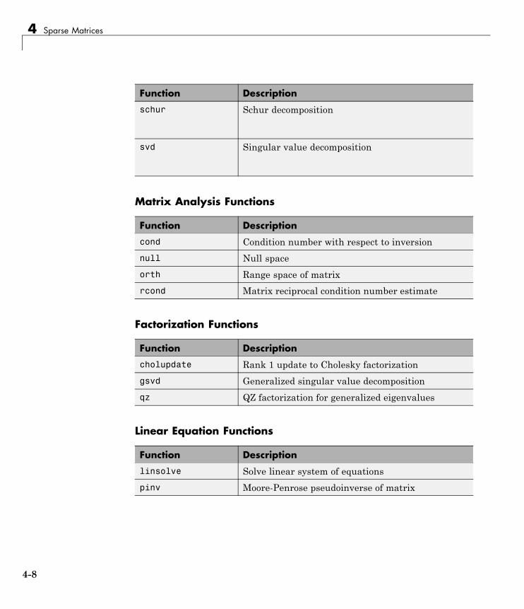
4 Sparse Matrices
Function Description
schur Schur decomposition
svd Singular value decomposition
Matrix Analysis Functions
Function Description
cond Condition number with respect to inversion
null Null space
orth Range space of matrix
rcond Matrix reciprocal condition number estimate
Factorization Functions
Function Description
cholupdate Rank 1 update to Cholesky factorization
gsvd Generalized singular value decomposition
qz QZ factorization for generalized eigenvalues
Linear Equation Functions
Function Description
linsolve Solve linear system of equations
pinv Moore-Penrose pseudoinverse of matrix
4-8
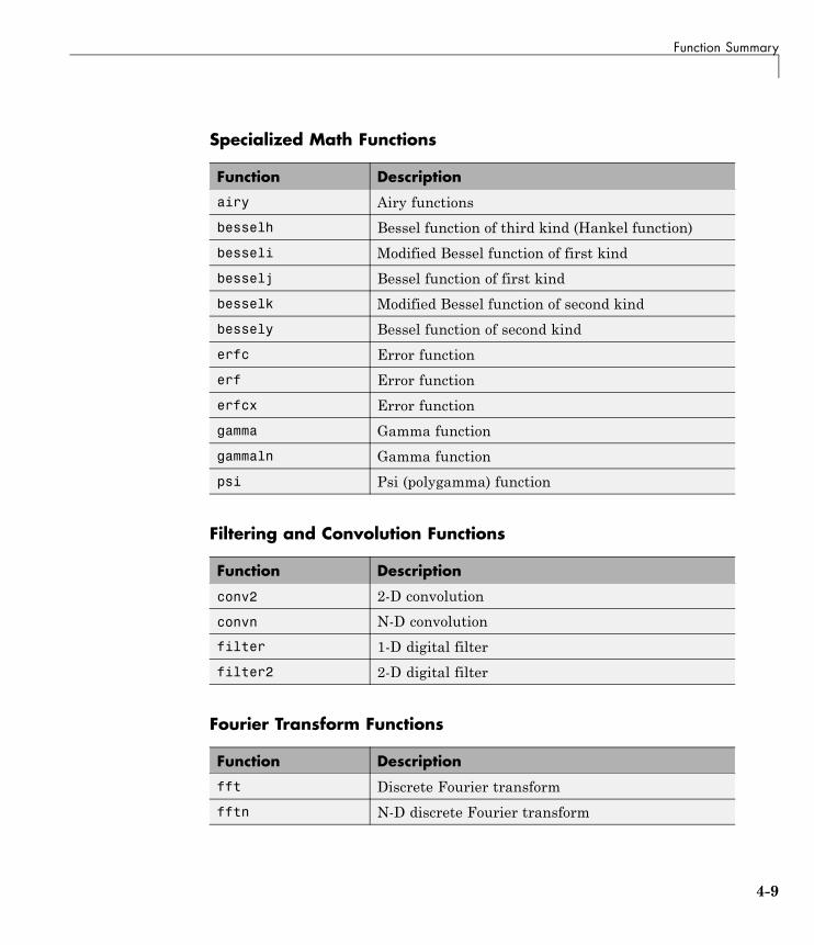
Function Summary
Specialized Math Functions
Function Description
airy Airy functions
besselh Bessel function of third kind (Hankel function)
besseli Modified Bessel function of first kind
besselj Bessel function of first kind
besselk Modified Bessel function of second kind
bessely Bessel function of second kind
erfc Error function
erf Error function
erfcx Error function
gamma Gamma function
gammaln Gamma function
psi Psi (polygamma) function
Filtering and Convolution Functions
Function Description
conv2 2-D convolution
convn N-D convolution
filter 1-D digital filter
filter2 2-D digital filter
Fourier Transform Functions
Function Description
fft Discrete Fourier transform
fftn N-D discrete Fourier transform
4-9
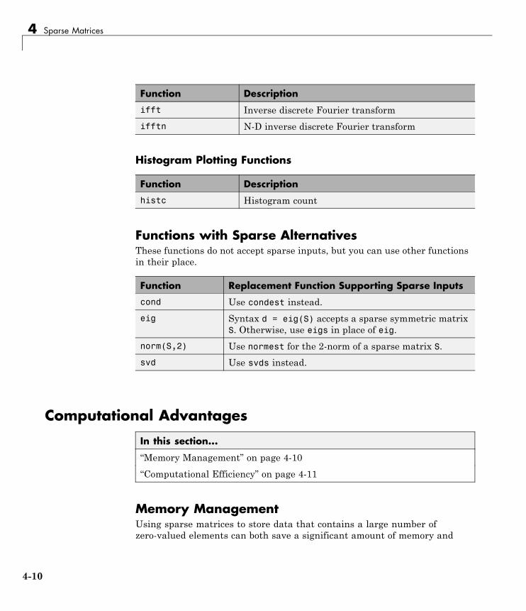
4 Sparse Matrices
Function Description
ifft Inverse discrete Fourier transform
ifftn N-D inverse discrete Fourier transform
Histogram Plotting Functions
Function Description
histc Histogram count
Functions with Sparse AlternativesThese functions do not accept sparse inputs, but you can use other functionsin their place.
Function Replacement Function Supporting Sparse Inputs
cond Use condest instead.
eig Syntax d = eig(S) accepts a sparse symmetric matrixS. Otherwise, use eigs in place of eig.
norm(S,2) Use normest for the 2-norm of a sparse matrix S.
svd Use svds instead.
Computational Advantages
In this section...
“Memory Management” on page 4-10
“Computational Efficiency” on page 4-11
Memory ManagementUsing sparse matrices to store data that contains a large number ofzero-valued elements can both save a significant amount of memory and
4-10
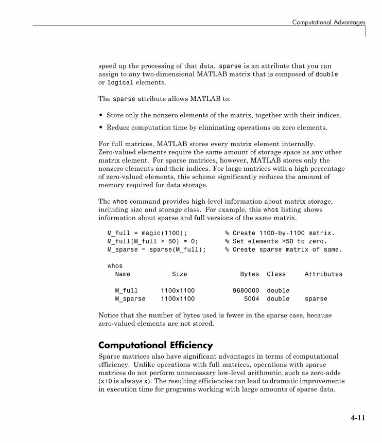
Computational Advantages
speed up the processing of that data. sparse is an attribute that you canassign to any two-dimensional MATLAB matrix that is composed of doubleor logical elements.
The sparse attribute allows MATLAB to:
• Store only the nonzero elements of the matrix, together with their indices.
• Reduce computation time by eliminating operations on zero elements.
For full matrices, MATLAB stores every matrix element internally.Zero-valued elements require the same amount of storage space as any othermatrix element. For sparse matrices, however, MATLAB stores only thenonzero elements and their indices. For large matrices with a high percentageof zero-valued elements, this scheme significantly reduces the amount ofmemory required for data storage.
The whos command provides high-level information about matrix storage,including size and storage class. For example, this whos listing showsinformation about sparse and full versions of the same matrix.
M_full = magic(1100); % Create 1100-by-1100 matrix.M_full(M_full > 50) = 0; % Set elements >50 to zero.M_sparse = sparse(M_full); % Create sparse matrix of same.
whosName Size Bytes Class Attributes
M_full 1100x1100 9680000 doubleM_sparse 1100x1100 5004 double sparse
Notice that the number of bytes used is fewer in the sparse case, becausezero-valued elements are not stored.
Computational EfficiencySparse matrices also have significant advantages in terms of computationalefficiency. Unlike operations with full matrices, operations with sparsematrices do not perform unnecessary low-level arithmetic, such as zero-adds(x+0 is always x). The resulting efficiencies can lead to dramatic improvementsin execution time for programs working with large amounts of sparse data.
4-11

4 Sparse Matrices
For more information, see “Sparse Matrix Operations” on page 4-25.
4-12
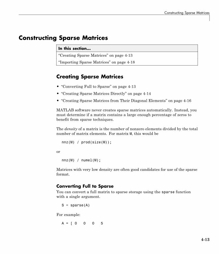
Constructing Sparse Matrices
Constructing Sparse Matrices
In this section...
“Creating Sparse Matrices” on page 4-13
“Importing Sparse Matrices” on page 4-18
Creating Sparse Matrices
• “Converting Full to Sparse” on page 4-13
• “Creating Sparse Matrices Directly” on page 4-14
• “Creating Sparse Matrices from Their Diagonal Elements” on page 4-16
MATLAB software never creates sparse matrices automatically. Instead, youmust determine if a matrix contains a large enough percentage of zeros tobenefit from sparse techniques.
The density of a matrix is the number of nonzero elements divided by the totalnumber of matrix elements. For matrix M, this would be
nnz(M) / prod(size(M));
or
nnz(M) / numel(M);
Matrices with very low density are often good candidates for use of the sparseformat.
Converting Full to SparseYou can convert a full matrix to sparse storage using the sparse functionwith a single argument.
S = sparse(A)
For example:
A = [ 0 0 0 5
4-13
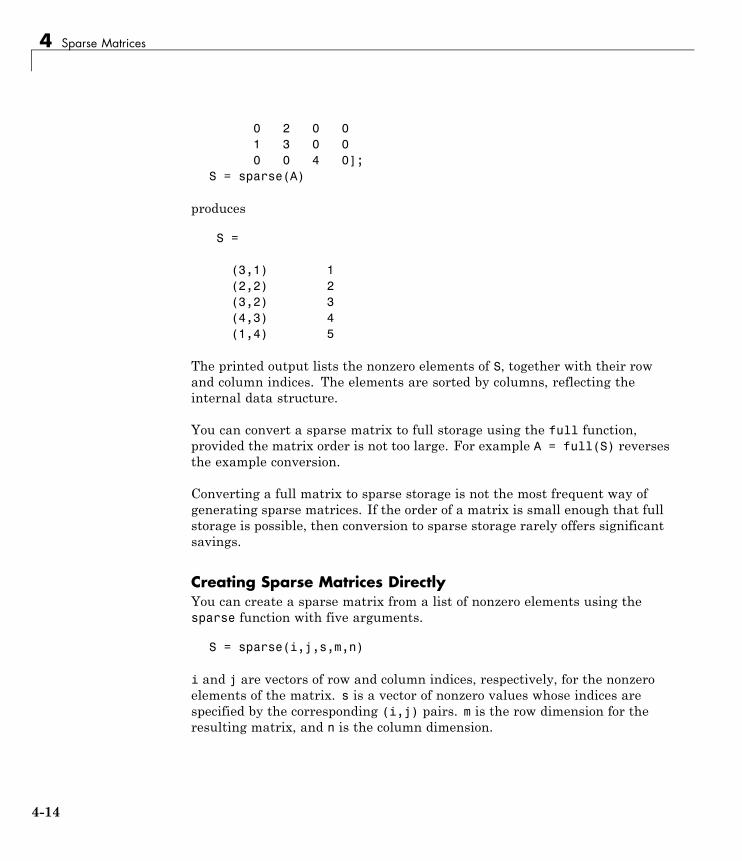
4 Sparse Matrices
0 2 0 01 3 0 00 0 4 0];
S = sparse(A)
produces
S =
(3,1) 1(2,2) 2(3,2) 3(4,3) 4(1,4) 5
The printed output lists the nonzero elements of S, together with their rowand column indices. The elements are sorted by columns, reflecting theinternal data structure.
You can convert a sparse matrix to full storage using the full function,provided the matrix order is not too large. For example A = full(S) reversesthe example conversion.
Converting a full matrix to sparse storage is not the most frequent way ofgenerating sparse matrices. If the order of a matrix is small enough that fullstorage is possible, then conversion to sparse storage rarely offers significantsavings.
Creating Sparse Matrices DirectlyYou can create a sparse matrix from a list of nonzero elements using thesparse function with five arguments.
S = sparse(i,j,s,m,n)
i and j are vectors of row and column indices, respectively, for the nonzeroelements of the matrix. s is a vector of nonzero values whose indices arespecified by the corresponding (i,j) pairs. m is the row dimension for theresulting matrix, and n is the column dimension.
4-14
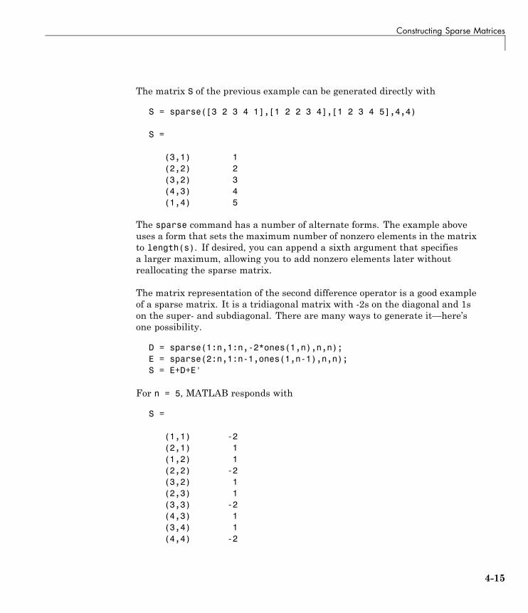
Constructing Sparse Matrices
The matrix S of the previous example can be generated directly with
S = sparse([3 2 3 4 1],[1 2 2 3 4],[1 2 3 4 5],4,4)
S =
(3,1) 1(2,2) 2(3,2) 3(4,3) 4(1,4) 5
The sparse command has a number of alternate forms. The example aboveuses a form that sets the maximum number of nonzero elements in the matrixto length(s). If desired, you can append a sixth argument that specifiesa larger maximum, allowing you to add nonzero elements later withoutreallocating the sparse matrix.
The matrix representation of the second difference operator is a good exampleof a sparse matrix. It is a tridiagonal matrix with -2s on the diagonal and 1son the super- and subdiagonal. There are many ways to generate it—here’sone possibility.
D = sparse(1:n,1:n,-2*ones(1,n),n,n);E = sparse(2:n,1:n-1,ones(1,n-1),n,n);S = E+D+E'
For n = 5, MATLAB responds with
S =
(1,1) -2(2,1) 1(1,2) 1(2,2) -2(3,2) 1(2,3) 1(3,3) -2(4,3) 1(3,4) 1(4,4) -2
4-15
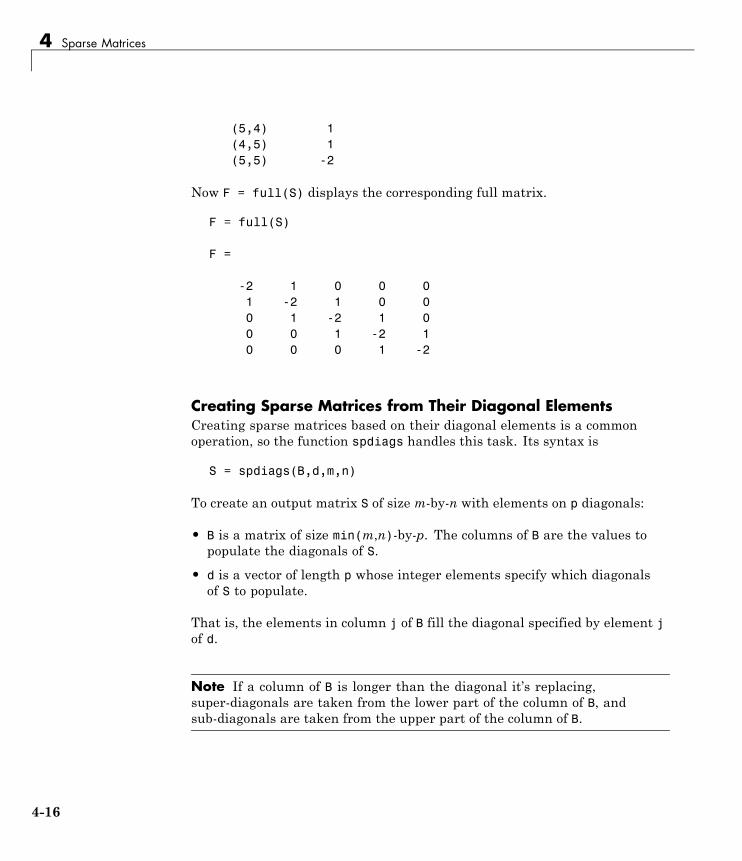
4 Sparse Matrices
(5,4) 1(4,5) 1(5,5) -2
Now F = full(S) displays the corresponding full matrix.
F = full(S)
F =
-2 1 0 0 01 -2 1 0 00 1 -2 1 00 0 1 -2 10 0 0 1 -2
Creating Sparse Matrices from Their Diagonal ElementsCreating sparse matrices based on their diagonal elements is a commonoperation, so the function spdiags handles this task. Its syntax is
S = spdiags(B,d,m,n)
To create an output matrix S of size m-by-n with elements on p diagonals:
• B is a matrix of size min(m,n)-by-p. The columns of B are the values topopulate the diagonals of S.
• d is a vector of length p whose integer elements specify which diagonalsof S to populate.
That is, the elements in column j of B fill the diagonal specified by element jof d.
Note If a column of B is longer than the diagonal it’s replacing,super-diagonals are taken from the lower part of the column of B, andsub-diagonals are taken from the upper part of the column of B.
4-16
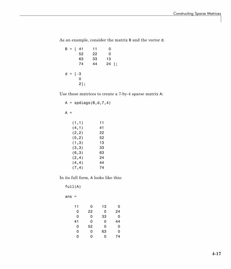
Constructing Sparse Matrices
As an example, consider the matrix B and the vector d.
B = [ 41 11 052 22 063 33 1374 44 24 ];
d = [-302];
Use these matrices to create a 7-by-4 sparse matrix A:
A = spdiags(B,d,7,4)
A =
(1,1) 11(4,1) 41(2,2) 22(5,2) 52(1,3) 13(3,3) 33(6,3) 63(2,4) 24(4,4) 44(7,4) 74
In its full form, A looks like this:
full(A)
ans =
11 0 13 00 22 0 240 0 33 0
41 0 0 440 52 0 00 0 63 00 0 0 74
4-17
4 Sparse Matrices
spdiags can also extract diagonal elements from a sparse matrix, or replacematrix diagonal elements with new values. Type help spdiags for details.
Importing Sparse MatricesYou can import sparse matrices from computations outside the MATLABenvironment. Use the spconvert function in conjunction with the loadcommand to import text files containing lists of indices and nonzero elements.For example, consider a three-column text file T.dat whose first column is alist of row indices, second column is a list of column indices, and third columnis a list of nonzero values. These statements load T.dat into MATLAB andconvert it into a sparse matrix S:
load T.datS = spconvert(T)
The save and load commands can also process sparse matrices stored asbinary data in MAT-files.
4-18
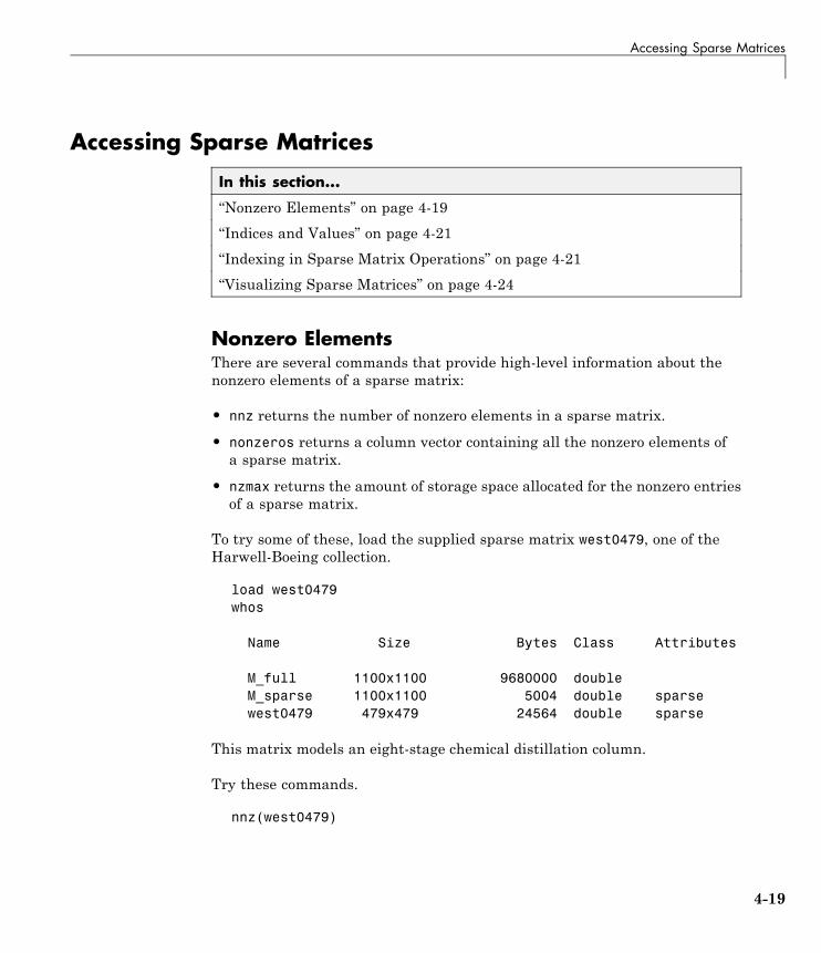
Accessing Sparse Matrices
Accessing Sparse Matrices
In this section...
“Nonzero Elements” on page 4-19
“Indices and Values” on page 4-21
“Indexing in Sparse Matrix Operations” on page 4-21
“Visualizing Sparse Matrices” on page 4-24
Nonzero ElementsThere are several commands that provide high-level information about thenonzero elements of a sparse matrix:
• nnz returns the number of nonzero elements in a sparse matrix.
• nonzeros returns a column vector containing all the nonzero elements ofa sparse matrix.
• nzmax returns the amount of storage space allocated for the nonzero entriesof a sparse matrix.
To try some of these, load the supplied sparse matrix west0479, one of theHarwell-Boeing collection.
load west0479whos
Name Size Bytes Class Attributes
M_full 1100x1100 9680000 doubleM_sparse 1100x1100 5004 double sparsewest0479 479x479 24564 double sparse
This matrix models an eight-stage chemical distillation column.
Try these commands.
nnz(west0479)
4-19
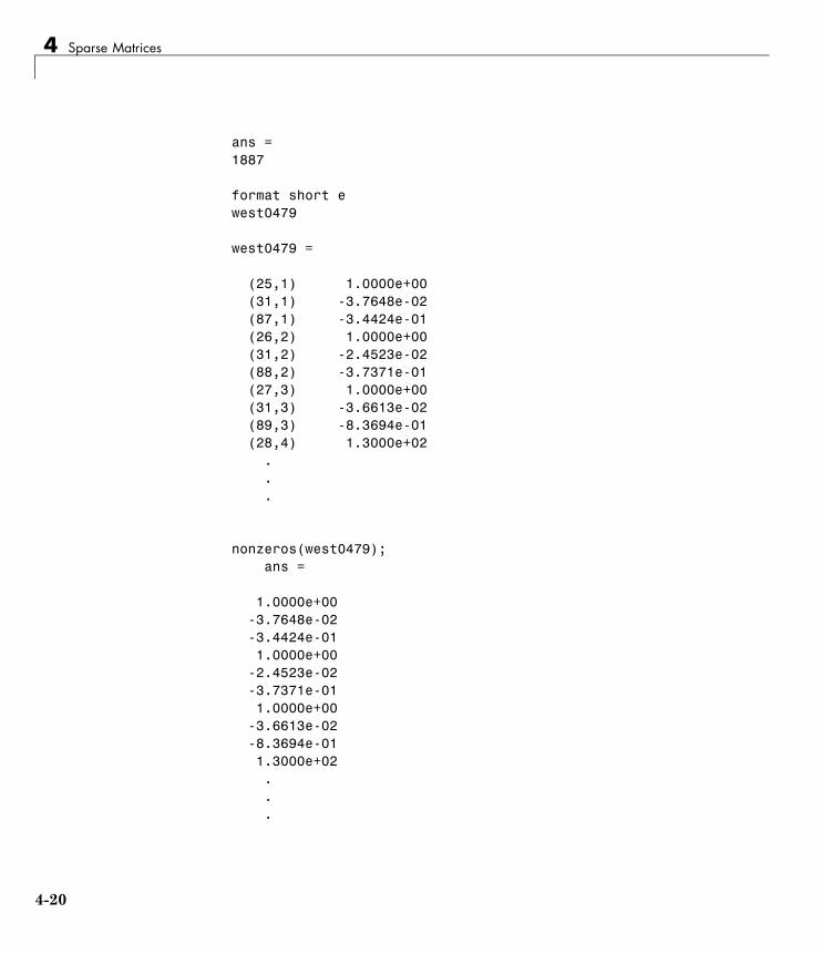
4 Sparse Matrices
ans =1887
format short ewest0479
west0479 =
(25,1) 1.0000e+00(31,1) -3.7648e-02(87,1) -3.4424e-01(26,2) 1.0000e+00(31,2) -2.4523e-02(88,2) -3.7371e-01(27,3) 1.0000e+00(31,3) -3.6613e-02(89,3) -8.3694e-01(28,4) 1.3000e+02
.
.
.
nonzeros(west0479);ans =
1.0000e+00-3.7648e-02-3.4424e-011.0000e+00
-2.4523e-02-3.7371e-011.0000e+00
-3.6613e-02-8.3694e-011.3000e+02...
4-20
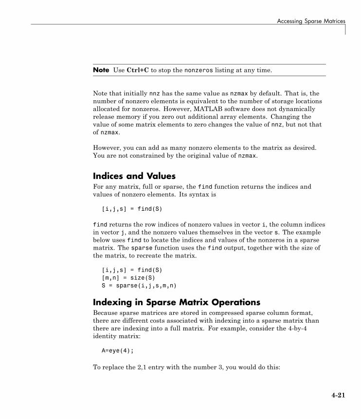
Accessing Sparse Matrices
Note Use Ctrl+C to stop the nonzeros listing at any time.
Note that initially nnz has the same value as nzmax by default. That is, thenumber of nonzero elements is equivalent to the number of storage locationsallocated for nonzeros. However, MATLAB software does not dynamicallyrelease memory if you zero out additional array elements. Changing thevalue of some matrix elements to zero changes the value of nnz, but not thatof nzmax.
However, you can add as many nonzero elements to the matrix as desired.You are not constrained by the original value of nzmax.
Indices and ValuesFor any matrix, full or sparse, the find function returns the indices andvalues of nonzero elements. Its syntax is
[i,j,s] = find(S)
find returns the row indices of nonzero values in vector i, the column indicesin vector j, and the nonzero values themselves in the vector s. The examplebelow uses find to locate the indices and values of the nonzeros in a sparsematrix. The sparse function uses the find output, together with the size ofthe matrix, to recreate the matrix.
[i,j,s] = find(S)[m,n] = size(S)S = sparse(i,j,s,m,n)
Indexing in Sparse Matrix OperationsBecause sparse matrices are stored in compressed sparse column format,there are different costs associated with indexing into a sparse matrix thanthere are indexing into a full matrix. For example, consider the 4-by-4identity matrix:
A=eye(4);
To replace the 2,1 entry with the number 3, you would do this:
4-21
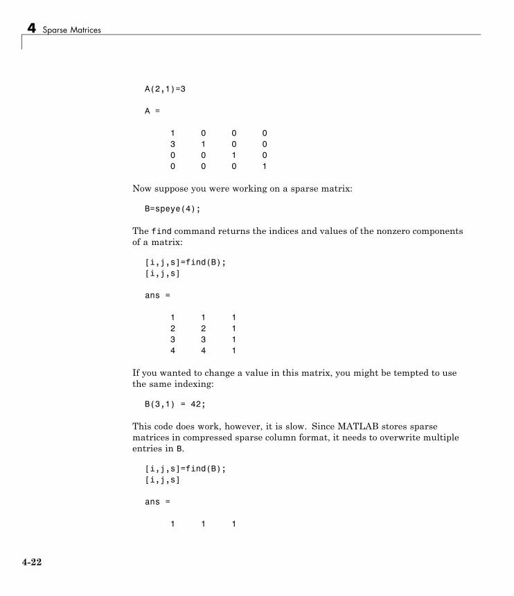
4 Sparse Matrices
A(2,1)=3
A =
1 0 0 03 1 0 00 0 1 00 0 0 1
Now suppose you were working on a sparse matrix:
B=speye(4);
The find command returns the indices and values of the nonzero componentsof a matrix:
[i,j,s]=find(B);[i,j,s]
ans =
1 1 12 2 13 3 14 4 1
If you wanted to change a value in this matrix, you might be tempted to usethe same indexing:
B(3,1) = 42;
This code does work, however, it is slow. Since MATLAB stores sparsematrices in compressed sparse column format, it needs to overwrite multipleentries in B.
[i,j,s]=find(B);[i,j,s]
ans =
1 1 1
4-22
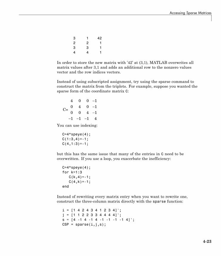
Accessing Sparse Matrices
3 1 422 2 13 3 14 4 1
In order to store the new matrix with ’42’ at (3,1), MATLAB overwrites allmatrix values after 3,1 and adds an additional row to the nonzero valuesvector and the row indices vectors.
Instead of using subscripted assignment, try using the sparse command toconstruct the matrix from the triplets. For example, suppose you wanted thesparse form of the coordinate matrix C:
C=
4 0 0 10 4 0 10 0 4 11 1 1 4
−−−
− − −
You can use indexing:
C=4*speye(4);C(1:3,4)=-1;C(4,1:3)=-1;
but this has the same issue that many of the entries in C need to beoverwritten. If you use a loop, you exacerbate the inefficiency:
C=4*speye(4);for k=1:3
C(k,4)=-1;C(4,k)=-1;
end
Instead of rewriting every matrix entry when you want to rewrite one,construct the three-column matrix directly with the sparse function:
i = [1 4 2 4 3 4 1 2 3 4]';j = [1 1 2 2 3 3 4 4 4 4]';s = [4 -1 4 -1 4 -1 -1 -1 -1 4]';CSP = sparse(i,j,s);
4-23
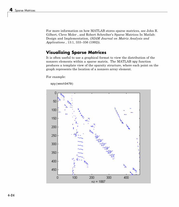
4 Sparse Matrices
For more information on how MATLAB stores sparse matrices, see John R.Gilbert, Cleve Moler , and Robert Schreiber’s Sparse Matrices In Matlab:Design and Implementation, (SIAM Journal on Matrix Analysis andApplications , 13:1, 333–356 (1992)).
Visualizing Sparse MatricesIt is often useful to use a graphical format to view the distribution of thenonzero elements within a sparse matrix. The MATLAB spy functionproduces a template view of the sparsity structure, where each point on thegraph represents the location of a nonzero array element.
For example:
spy(west0479)
4-24
Sparse Matrix Operations
Sparse Matrix Operations
In this section...
“Efficiency of Operations” on page 4-25
“Permutations and Reordering” on page 4-26
“Factoring Sparse Matrices” on page 4-30
“Systems of Linear Equations” on page 4-37
“Eigenvalues and Singular Values” on page 4-40
“Performance Limitations” on page 4-42
Efficiency of Operations
• “Computational Complexity” on page 4-25
• “Algorithmic Details” on page 4-25
Computational ComplexityThe computational complexity of sparse operations is proportional to nnz,the number of nonzero elements in the matrix. Computational complexityalso depends linearly on the row size m and column size n of the matrix, butis independent of the product m*n, the total number of zero and nonzeroelements.
The complexity of fairly complicated operations, such as the solution of sparselinear equations, involves factors like ordering and fill-in, which are discussedin the previous section. In general, however, the computer time requiredfor a sparse matrix operation is proportional to the number of arithmeticoperations on nonzero quantities.
Algorithmic DetailsSparse matrices propagate through computations according to these rules:
• Functions that accept a matrix and return a scalar or constant-size vectoralways produce output in full storage format. For example, the sizefunction always returns a full vector, whether its input is full or sparse.
4-25
4 Sparse Matrices
• Functions that accept scalars or vectors and return matrices, such aszeros, ones, rand, and eye, always return full results. This is necessary toavoid introducing sparsity unexpectedly. The sparse analog of zeros(m,n)is simply sparse(m,n). The sparse analogs of rand and eye are sprand andspeye, respectively. There is no sparse analog for the function ones.
• Unary functions that accept a matrix and return a matrix or vector preservethe storage class of the operand. If S is a sparse matrix, then chol(S) isalso a sparse matrix, and diag(S) is a sparse vector. Columnwise functionssuch as max and sum also return sparse vectors, even though these vectorscan be entirely nonzero. Important exceptions to this rule are the sparseand full functions.
• Binary operators yield sparse results if both operands are sparse, and fullresults if both are full. For mixed operands, the result is full unless theoperation preserves sparsity. If S is sparse and F is full, then S+F, S*F, andF\S are full, while S.*F and S&F are sparse. In some cases, the result mightbe sparse even though the matrix has few zero elements.
• Matrix concatenation using either the cat function or square bracketsproduces sparse results for mixed operands.
• Submatrix indexing on the right side of an assignment preserves thestorage format of the operand unless the result is a scalar. T = S(i,j)produces a sparse result if S is sparse and either i or j is a vector. Itproduces a full scalar if both i and j are scalars. Submatrix indexing onthe left, as in T(i,j) = S, does not change the storage format of the matrixon the left.
Permutations and Reordering
• “Reordering for Sparsity” on page 4-29
• “Reordering to Reduce Bandwidth” on page 4-29
• “Approximate Minimum Degree Ordering” on page 4-29
A permutation of the rows and columns of a sparse matrix S can berepresented in two ways:
• A permutation matrix P acts on the rows of S as P*S or on the columnsas S*P'.
4-26
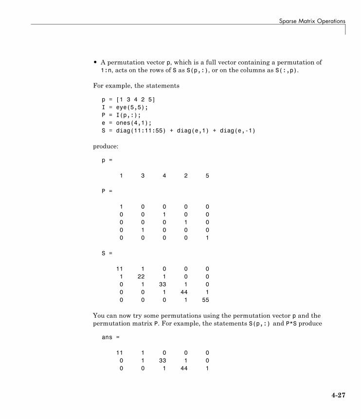
Sparse Matrix Operations
• A permutation vector p, which is a full vector containing a permutation of1:n, acts on the rows of S as S(p,:), or on the columns as S(:,p).
For example, the statements
p = [1 3 4 2 5]I = eye(5,5);P = I(p,:);e = ones(4,1);S = diag(11:11:55) + diag(e,1) + diag(e,-1)
produce:
p =
1 3 4 2 5
P =
1 0 0 0 00 0 1 0 00 0 0 1 00 1 0 0 00 0 0 0 1
S =
11 1 0 0 01 22 1 0 00 1 33 1 00 0 1 44 10 0 0 1 55
You can now try some permutations using the permutation vector p and thepermutation matrix P. For example, the statements S(p,:) and P*S produce
ans =
11 1 0 0 00 1 33 1 00 0 1 44 1
4-27

4 Sparse Matrices
1 22 1 0 00 0 0 1 55
Similarly, S(:,p) and S*P' produce
ans =
11 0 0 1 01 1 0 22 00 33 1 1 00 1 44 0 10 0 1 0 55
If P is a sparse matrix, then both representations use storage proportionalto n and you can apply either to S in time proportional to nnz(S). The vectorrepresentation is slightly more compact and efficient, so the various sparsematrix permutation routines all return full row vectors with the exception ofthe pivoting permutation in LU (triangular) factorization, which returns amatrix compatible with the full LU factorization.
To convert between the two representations, let I = speye(n) be an identitymatrix of the appropriate size. Then,
P = I(p,:)P' = I(:,p)p = (1:n)*P'p = (P*(1:n)')'
The inverse of P is simply R = P'. You can compute the inverse of p withr(p) = 1:n.
r(p) = 1:5
r =
1 4 2 3 5
4-28
Sparse Matrix Operations
Reordering for SparsityReordering the columns of a matrix can often make its LU or QR factorssparser. Reordering the rows and columns can often make its Choleskyfactors sparser. The simplest such reordering is to sort the columns bynonzero count. This is sometimes a good reordering for matrices with veryirregular structures, especially if there is great variation in the nonzerocounts of rows or columns.
The function p = colperm(S) computes this column-count permutation. Thecolperm code has only a single line.
[ignore,p] = sort(sum(spones(S)));
This line performs these steps:
1 The inner call to spones creates a sparse matrix with ones at the locationof every nonzero element in S.
2 The sum function sums down the columns of the matrix, producing a vectorthat contains the count of nonzeros in each column.
3 full converts this vector to full storage format.
4 sort sorts the values in ascending order. The second output argument fromsort is the permutation that sorts this vector.
Reordering to Reduce BandwidthThe reverse Cuthill-McKee ordering is intended to reduce the profile orbandwidth of the matrix. It is not guaranteed to find the smallest possiblebandwidth, but it usually does. The function symrcm(A) actually operates onthe nonzero structure of the symmetric matrix A + A', but the result is alsouseful for asymmetric matrices. This ordering is useful for matrices thatcome from one-dimensional problems or problems that are in some sense“long and thin.”
Approximate Minimum Degree OrderingThe degree of a node in a graph is the number of connections to that node.This is the same as the number of off-diagonal nonzero elements in thecorresponding row of the adjacency matrix. The approximate minimum
4-29
4 Sparse Matrices
degree algorithm generates an ordering based on how these degrees arealtered during Gaussian elimination or Cholesky factorization. It is acomplicated and powerful algorithm that usually leads to sparser factors thanmost other orderings, including column count and reverse Cuthill-McKee.Because the keeping track of the degree of each node is very time-consuming,the approximate minimum degree algorithm uses an approximation to thedegree, rather than the exact degree.
The following MATLAB functions implement the approximate minimumdegree algorithm:
• symamd — Use with symmetric matrices.
• colamd — Use with nonsymmetric matrices and symmetric matrices ofthe form A*A' or A'*A.
See “Reordering and Factorization” on page 4-31 for an example using symamd.
You can change various parameters associated with details of the algorithmsusing the spparms function.
For details on the algorithms used by colamd and symamd, see [5]. Theapproximate degree the algorithms use is based on [1].
Factoring Sparse Matrices
• “LU Factorization” on page 4-30
• “Cholesky Factorization” on page 4-33
• “QR Factorization” on page 4-34
• “Incomplete Factorizations” on page 4-35
LU FactorizationIf S is a sparse matrix, the following command returns three sparse matricesL, U, and P such that P*S = L*U.
[L,U,P] = lu(S)
4-30
Sparse Matrix Operations
lu obtains the factors by Gaussian elimination with partial pivoting. Thepermutation matrix P has only n nonzero elements. As with dense matrices,the statement [L,U] = lu(S) returns a permuted unit lower triangularmatrix and an upper triangular matrix whose product is S. By itself, lu(S)returns L and U in a single matrix without the pivot information.
The three-output syntax
[L,U,P] = lu(S)
selects P via numerical partial pivoting, but does not pivot to improve sparsityin the LU factors. On the other hand, the four-output syntax
[L,U,P,Q]=lu(S)
selects P via threshold partial pivoting, and selects P and Q to improve sparsityin the LU factors.
You can control pivoting in sparse matrices using
lu(S,thresh)
where thresh is a pivot threshold in [0,1]. Pivoting occurs when the diagonalentry in a column has magnitude less than thresh times the magnitude ofany sub-diagonal entry in that column. thresh = 0 forces diagonal pivoting.thresh = 1 is the default. (The default for thresh is 0.1 for the four-outputsyntax).
When you call lu with three or less outputs, MATLAB automaticallyallocates the memory necessary to hold the sparse L and U factors during thefactorization. Except for the four-output syntax, MATLAB does not use anysymbolic LU prefactorization to determine the memory requirements and setup the data structures in advance.
Reordering and Factorization. If you obtain a good column permutationp that reduces fill-in, perhaps from symrcm or colamd, then computinglu(S(:,p)) takes less time and storage than computing lu(S). Twopermutations are the symmetric reverse Cuthill-McKee ordering and thesymmetric approximate minimum degree ordering.
r = symrcm(B);
4-31
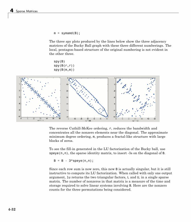
4 Sparse Matrices
m = symamd(B);
The three spy plots produced by the lines below show the three adjacencymatrices of the Bucky Ball graph with these three different numberings. Thelocal, pentagon-based structure of the original numbering is not evident inthe other three.
spy(B)spy(B(r,r))spy(B(m,m))
The reverse Cuthill-McKee ordering, r, reduces the bandwidth andconcentrates all the nonzero elements near the diagonal. The approximateminimum degree ordering, m, produces a fractal-like structure with largeblocks of zeros.
To see the fill-in generated in the LU factorization of the Bucky ball, usespeye(n,n), the sparse identity matrix, to insert -3s on the diagonal of B.
B = B - 3*speye(n,n);
Since each row sum is now zero, this new B is actually singular, but it is stillinstructive to compute its LU factorization. When called with only one outputargument, lu returns the two triangular factors, L and U, in a single sparsematrix. The number of nonzeros in that matrix is a measure of the time andstorage required to solve linear systems involving B. Here are the nonzerocounts for the three permutations being considered.
4-32
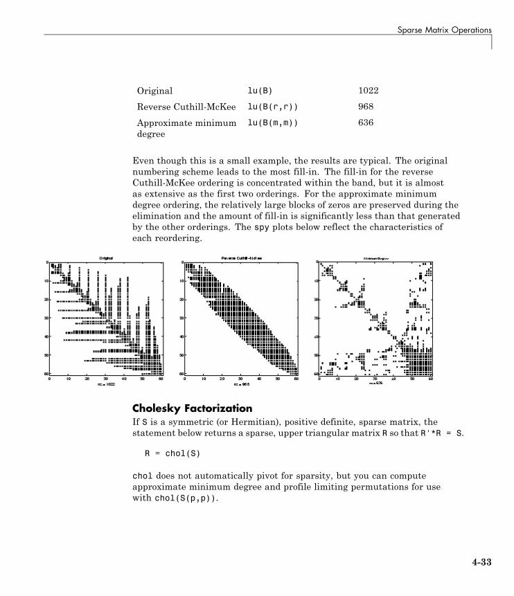
Sparse Matrix Operations
Original lu(B) 1022
Reverse Cuthill-McKee lu(B(r,r)) 968
Approximate minimumdegree
lu(B(m,m)) 636
Even though this is a small example, the results are typical. The originalnumbering scheme leads to the most fill-in. The fill-in for the reverseCuthill-McKee ordering is concentrated within the band, but it is almostas extensive as the first two orderings. For the approximate minimumdegree ordering, the relatively large blocks of zeros are preserved during theelimination and the amount of fill-in is significantly less than that generatedby the other orderings. The spy plots below reflect the characteristics ofeach reordering.
Cholesky FactorizationIf S is a symmetric (or Hermitian), positive definite, sparse matrix, thestatement below returns a sparse, upper triangular matrix R so that R'*R = S.
R = chol(S)
chol does not automatically pivot for sparsity, but you can computeapproximate minimum degree and profile limiting permutations for usewith chol(S(p,p)).
4-33
4 Sparse Matrices
Since the Cholesky algorithm does not use pivoting for sparsity and does notrequire pivoting for numerical stability, chol does a quick calculation of theamount of memory required and allocates all the memory at the start of thefactorization. You can use symbfact, which uses the same algorithm as chol,to calculate how much memory is allocated.
QR FactorizationMATLAB computes the complete QR factorization of a sparse matrix S with
[Q,R] = qr(S)
or
[Q,R,E] = qr(S)
but this is often impractical. The unitary matrix Q often fails to have a highproportion of zero elements. A more practical alternative, sometimes knownas “the Q-less QR factorization,” is available.
With one sparse input argument and one output argument
R = qr(S)
returns just the upper triangular portion of the QR factorization. The matrixR provides a Cholesky factorization for the matrix associated with the normalequations:
R'*R = S'*S
However, the loss of numerical information inherent in the computation ofS'*S is avoided.
With two input arguments having the same number of rows, and two outputarguments, the statement
[C,R] = qr(S,B)
applies the orthogonal transformations to B, producing C = Q'*B withoutcomputing Q.
4-34
Sparse Matrix Operations
The Q-less QR factorization allows the solution of sparse least squaresproblems
minimize Ax b-2
with two steps
[c,R] = qr(A,b)x = R\c
If A is sparse, but not square, MATLAB uses these steps for the linearequation solving backslash operator:
x = A\b
Or, you can do the factorization yourself and examine R for rank deficiency.
It is also possible to solve a sequence of least squares linear systems withdifferent right-hand sides, b, that are not necessarily known when R = qr(A)is computed. The approach solves the “semi-normal equations”
R'*R*x = A'*b
with
x = R\(R'\(A'*b))
and then employs one step of iterative refinement to reduce round off error:
r = b - A*xe = R\(R'\(A'*r))x = x + e
Incomplete FactorizationsThe luinc, ilu, and cholinc functions provide approximate, incompletefactorizations, which are useful as preconditioners for sparse iterativemethods.
4-35
4 Sparse Matrices
The luinc function produces two different kinds of incomplete LU (ILU)factorizations, one involving a drop tolerance and one involving fill-in level.The ilu function produces three incomplete LU factorizations, the ILU withlevel 0 fill-in (ILU(0)), the Crout version of ILU (ILUC), and the ILU withthreshold and pivoting (ILUTP).
For example:
A = gallery('neumann', 1600) + speye(1600);nnz(A)ans =
7840
nnz(lu(A))ans =
126478
shows that A has 7840 nonzeros, and its complete LU factorization has126478 nonzeros:
nnz(luinc(A,'0'))ans =
7840
setup.type = 'nofill';nnz(ilu(A,setup))ans =
7840
nnz(luinc(A,1e-6))ans =
51541
setup.type = 'ilutp';setup.droptol = 1e-6;nnz(luinc(A,setup))ans =
51541
4-36
Sparse Matrix Operations
These calculations, with both the luinc and ilu functions, show that withlevel 0 fill-in it has 7840 nonzeros, and with a drop tolerance of 1e-6 it has51541 nonzeros. See the luinc and ilu reference pages for more optionsand details.
The cholinc function provides drop tolerance and level 0 fill-in Choleskyfactorizations of symmetric, positive definite sparse matrices. See the cholincreference page for more information.
Systems of Linear EquationsThere are two different classes of methods for solving systems of simultaneouslinear equations:
• Direct methods are usually variants of Gaussian elimination. Thesemethods involve the individual matrix elements directly, through matrixoperations such as LU or Cholesky factorization. MATLAB implementsdirect methods through the matrix division operators / and \, which youcan use to solve linear systems.
• Iterative methods produce only an approximate solution after a finitenumber of steps. These methods involve the coefficient matrix onlyindirectly, through a matrix-vector product or an abstract linear operator.Iterative methods are usually applied only to sparse matrices.
Direct MethodsDirect methods are usually faster and more generally applicable than indirectmethods, if there is enough storage available to carry them out. Iterativemethods are usually applicable to restricted cases of equations and dependon properties like diagonal dominance or the existence of an underlyingdifferential operator. Direct methods are implemented in the core of theMATLAB software and are made as efficient as possible for general classes ofmatrices. Iterative methods are usually implemented in MATLAB-languagefiles and can use the direct solution of subproblems or preconditioners.
4-37
4 Sparse Matrices
Using a Different Preordering. If A is not diagonal, banded, triangular,or a permutation of a triangular matrix, backslash (\) reorders the indicesof A to reduce the amount of fill-in—that is, the number of nonzero entriesthat are added to the sparse factorization matrices. The new ordering, calleda preordering, is performed before the factorization of A. In some cases, youmight be able to provide a better preordering than the one used by thebackslash algorithm.
To use a different preordering, first turn off both of the automatic preorderingsthat backslash might perform by default, using the function spparms asfollows:
spparms('autoamd',0);spparms('autommd',0);
Now, assuming you have created a permutation vector p that specifies apreordering of the indices of A, apply backslash to the matrix A(:,p), whosecolumns are the columns of A, permuted according to the vector p.
x = A (:,p) \ b;x(p) = x;spparms('autoamd',1);spparms('autommd',1);
The commands spparms('autoamd',1) and spparms('autommd',1) turnsthe automatic preordering back on, in case you use A\b later withoutspecifying an appropriate preordering.
Iterative MethodsNine functions are available that implement iterative methods for sparsesystems of simultaneous linear systems.
Functions for Iterative Methods for Sparse Systems
Function Method
bicg Biconjugate gradient
bicgstab Biconjugate gradient stabilized
cgs Conjugate gradient squared
4-38

Sparse Matrix Operations
Functions for Iterative Methods for Sparse Systems (Continued)
Function Method
gmres Generalized minimum residual
lsqr Least squares
minres Minimum residual
pcg Preconditioned conjugate gradient
qmr Quasiminimal residual
symmlq Symmetric LQ
These methods are designed to solve Ax = b or minimize the norm of b –Ax. For the Preconditioned Conjugate Gradient method, pcg, A must be asymmetric, positive definite matrix. minres and symmlq can be used onsymmetric indefinite matrices. For lsqr, the matrix need not be square. Theother five can handle nonsymmetric, square matrices.
All nine methods can make use of preconditioners. The linear system
is replaced by the equivalent system
The preconditioner M is chosen to accelerate convergence of the iterativemethod. In many cases, the preconditioners occur naturally in themathematical model. A partial differential equation with variable coefficientscan be approximated by one with constant coefficients, for example.Incomplete matrix factorizations can be used in the absence of naturalpreconditioners.
The five-point finite difference approximation to Laplace’s equation ona square, two-dimensional domain provides an example. The followingstatements use the preconditioned conjugate gradient method preconditionerM = R’*R, where R is the incomplete Cholesky factor of A.
A = delsq(numgrid('S',50));
4-39
4 Sparse Matrices
b = ones(size(A,1),1);tol = 1.e-3;maxit = 10;R = cholinc(A,tol);[x,flag,err,iter,res] = pcg(A,b,tol,maxit,R',R);
Only four iterations are required to achieve the prescribed accuracy.
Background information on these iterative methods and incompletefactorizations is available in [2] and [7].
Eigenvalues and Singular ValuesTwo functions are available that compute a few specified eigenvalues orsingular values. svds is based on eigs that uses ARPACK [6].
Functions to Compute a Few Eigenvalues or Singular Values
Function Description
eigs Few eigenvalues
svds Few singular values
These functions are most frequently used with sparse matrices, but they canbe used with full matrices or even with linear operators defined in MATLABcode.
The statement
[V,lambda] = eigs(A,k,sigma)
finds the k eigenvalues and corresponding eigenvectors of the matrix A thatare nearest the “shift” sigma. If sigma is omitted, the eigenvalues largest inmagnitude are found. If sigma is zero, the eigenvalues smallest in magnitudeare found. A second matrix, B, can be included for the generalized eigenvalueproblem: Aυ = λBυ.
The statement
[U,S,V] = svds(A,k)
4-40
Sparse Matrix Operations
finds the k largest singular values of A and
[U,S,V] = svds(A,k,0)
finds the k smallest singular values.
For example, the statements
L = numgrid('L',65);A = delsq(L);
set up the five-point Laplacian difference operator on a 65-by-65 grid in anL-shaped, two-dimensional domain. The statements
size(A)nnz(A)
show that A is a matrix of order 2945 with 14,473 nonzero elements.
The statement
[v,d] = eigs(A,1,0);
computes the smallest eigenvalue and eigenvector. Finally,
L(L>0) = full(v(L(L>0)));x = -1:1/32:1;contour(x,x,L,15)axis square
distributes the components of the eigenvector over the appropriate grid pointsand produces a contour plot of the result.
4-41
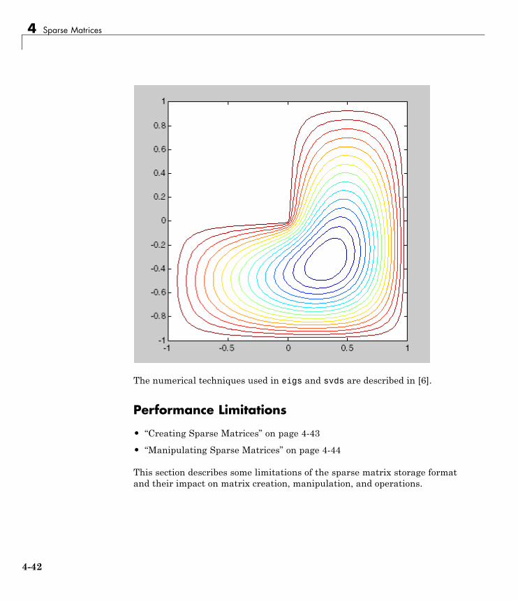
4 Sparse Matrices
The numerical techniques used in eigs and svds are described in [6].
Performance Limitations
• “Creating Sparse Matrices” on page 4-43
• “Manipulating Sparse Matrices” on page 4-44
This section describes some limitations of the sparse matrix storage formatand their impact on matrix creation, manipulation, and operations.
4-42
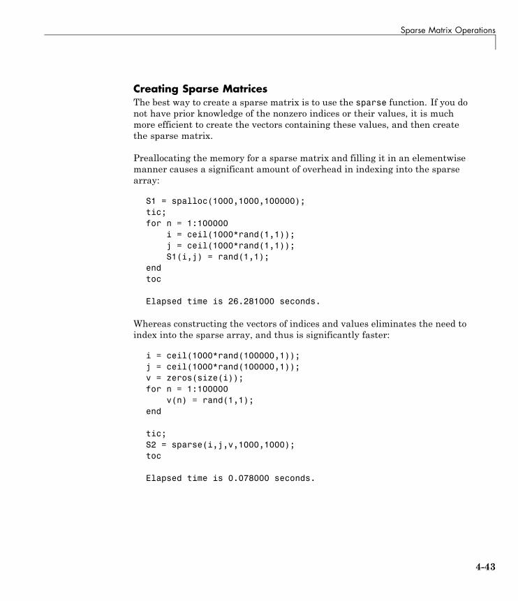
Sparse Matrix Operations
Creating Sparse MatricesThe best way to create a sparse matrix is to use the sparse function. If you donot have prior knowledge of the nonzero indices or their values, it is muchmore efficient to create the vectors containing these values, and then createthe sparse matrix.
Preallocating the memory for a sparse matrix and filling it in an elementwisemanner causes a significant amount of overhead in indexing into the sparsearray:
S1 = spalloc(1000,1000,100000);tic;for n = 1:100000
i = ceil(1000*rand(1,1));j = ceil(1000*rand(1,1));S1(i,j) = rand(1,1);
endtoc
Elapsed time is 26.281000 seconds.
Whereas constructing the vectors of indices and values eliminates the need toindex into the sparse array, and thus is significantly faster:
i = ceil(1000*rand(100000,1));j = ceil(1000*rand(100000,1));v = zeros(size(i));for n = 1:100000
v(n) = rand(1,1);end
tic;S2 = sparse(i,j,v,1000,1000);toc
Elapsed time is 0.078000 seconds.
4-43
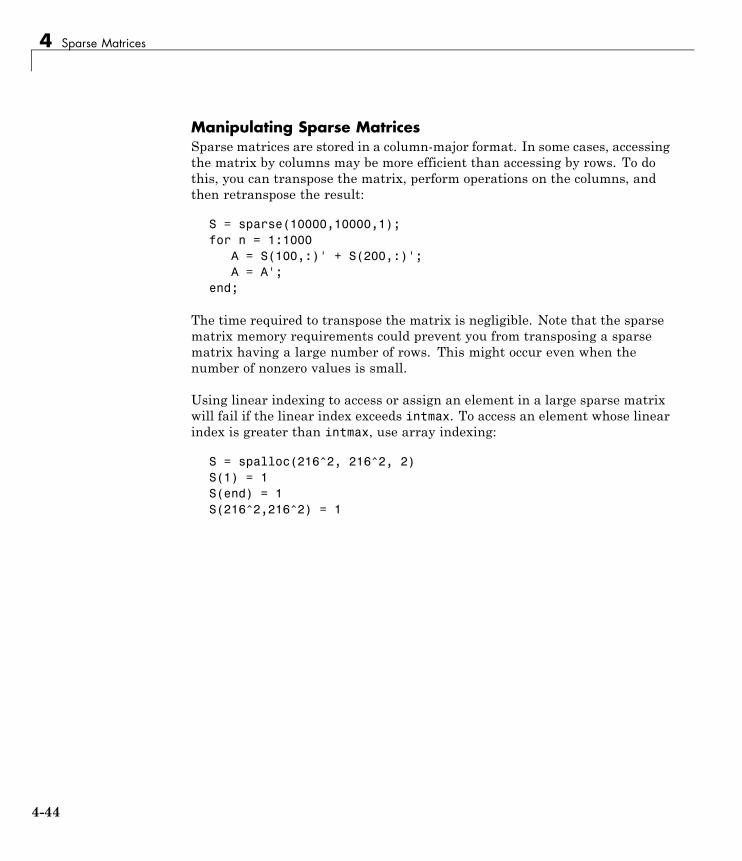
4 Sparse Matrices
Manipulating Sparse MatricesSparse matrices are stored in a column-major format. In some cases, accessingthe matrix by columns may be more efficient than accessing by rows. To dothis, you can transpose the matrix, perform operations on the columns, andthen retranspose the result:
S = sparse(10000,10000,1);for n = 1:1000
A = S(100,:)' + S(200,:)';A = A';
end;
The time required to transpose the matrix is negligible. Note that the sparsematrix memory requirements could prevent you from transposing a sparsematrix having a large number of rows. This might occur even when thenumber of nonzero values is small.
Using linear indexing to access or assign an element in a large sparse matrixwill fail if the linear index exceeds intmax. To access an element whose linearindex is greater than intmax, use array indexing:
S = spalloc(216^2, 216^2, 2)S(1) = 1S(end) = 1S(216^2,216^2) = 1
4-44
Selected Bibliography
Selected Bibliography[1] Amestoy, P. R., T. A. Davis, and I. S. Duff, “An Approximate MinimumDegree Ordering Algorithm,” SIAM Journal on Matrix Analysis andApplications, Vol. 17, No. 4, Oct. 1996, pp. 886-905.
[2] Barrett, R., M. Berry, T. F. Chan, et al., Templates for the Solution ofLinear Systems: Building Blocks for Iterative Methods, SIAM, Philadelphia,1994.
[3] Davis, T.A., Gilbert, J. R., Larimore, S.I., Ng, E., Peyton, B., “A ColumnApproximate Minimum Degree Ordering Algorithm,” Proc. SIAM Conferenceon Applied Linear Algebra, Oct. 1997, p. 29.
[4] Gilbert, John R., Cleve Moler, and Robert Schreiber, “Sparse Matrices inMATLAB: Design and Implementation,” SIAM J. Matrix Anal. Appl., Vol. 13,No. 1, January 1992, pp. 333-356.
[5] Larimore, S. I., An Approximate Minimum Degree Column OrderingAlgorithm, MS Thesis, Dept. of Computer and Information Science andEngineering, University of Florida, Gainesville, FL, 1998, available athttp://www.cise.ufl.edu/submit/files/file_281.ps .
[6] Lehoucq, R. B., D. C. Sorensen, C. Yang, ARPACK Users’ Guide, SIAM,Philadelphia, 1998.
[7] Saad, Yousef, Iterative Methods for Sparse Linear Equations. PWSPublishing Company, 1996.
4-45

4 Sparse Matrices
4-46

5
Functions of One Variable
• “Function Summary” on page 5-2
• “Representing Polynomials” on page 5-3
• “Evaluating Polynomials” on page 5-4
• “Roots of Polynomials” on page 5-5
• “Roots of Scalar Functions” on page 5-6
• “Derivatives” on page 5-12
• “Convolution” on page 5-13
• “Partial Fraction Expansions” on page 5-14
• “Polynomial Curve Fitting” on page 5-15
• “Characteristic Polynomials” on page 5-17
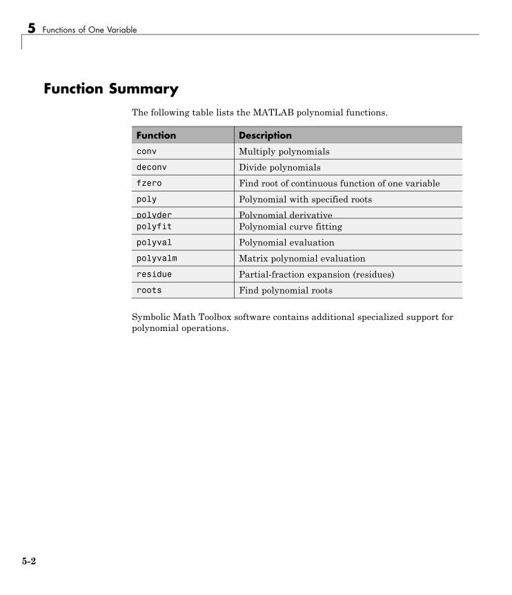
5 Functions of One Variable
Function SummaryThe following table lists the MATLAB polynomial functions.
Function Description
conv Multiply polynomials
deconv Divide polynomials
fzero Find root of continuous function of one variable
poly Polynomial with specified roots
polyder Polynomial derivativepolyfit Polynomial curve fitting
polyval Polynomial evaluation
polyvalm Matrix polynomial evaluation
residue Partial-fraction expansion (residues)
roots Find polynomial roots
Symbolic Math Toolbox software contains additional specialized support forpolynomial operations.
5-2
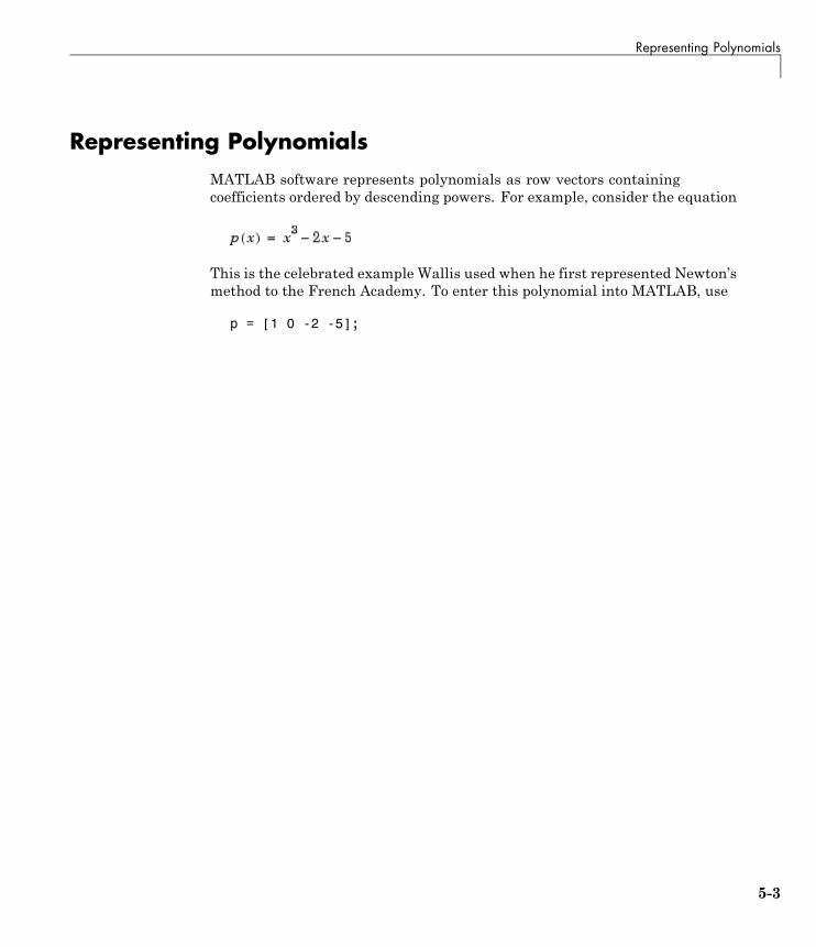
Representing Polynomials
Representing PolynomialsMATLAB software represents polynomials as row vectors containingcoefficients ordered by descending powers. For example, consider the equation
This is the celebrated example Wallis used when he first represented Newton’smethod to the French Academy. To enter this polynomial into MATLAB, use
p = [1 0 -2 -5];
5-3
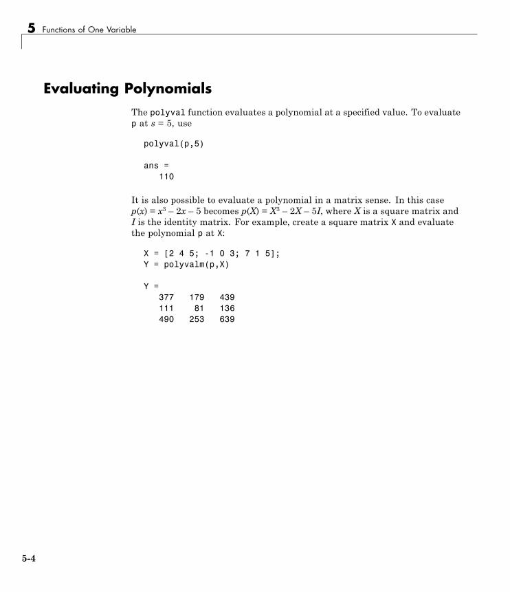
5 Functions of One Variable
Evaluating PolynomialsThe polyval function evaluates a polynomial at a specified value. To evaluatep at s = 5, use
polyval(p,5)
ans =110
It is also possible to evaluate a polynomial in a matrix sense. In this casep(x) = x3 – 2x – 5 becomes p(X) = X3 – 2X – 5I, where X is a square matrix andI is the identity matrix. For example, create a square matrix X and evaluatethe polynomial p at X:
X = [2 4 5; -1 0 3; 7 1 5];Y = polyvalm(p,X)
Y =377 179 439111 81 136490 253 639
5-4
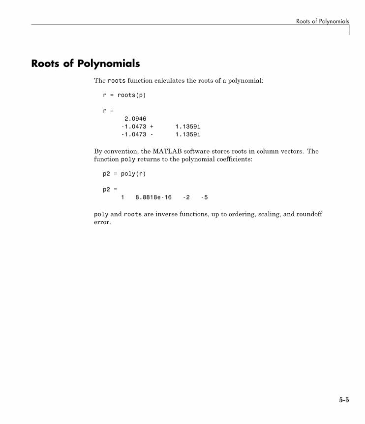
Roots of Polynomials
Roots of PolynomialsThe roots function calculates the roots of a polynomial:
r = roots(p)
r =2.0946
-1.0473 + 1.1359i-1.0473 - 1.1359i
By convention, the MATLAB software stores roots in column vectors. Thefunction poly returns to the polynomial coefficients:
p2 = poly(r)
p2 =1 8.8818e-16 -2 -5
poly and roots are inverse functions, up to ordering, scaling, and roundofferror.
5-5
5 Functions of One Variable
Roots of Scalar Functions
In this section...
“Solving a Nonlinear Equation in One Variable” on page 5-6
“Using a Starting Interval” on page 5-8
“Using a Starting Point” on page 5-9
Solving a Nonlinear Equation in One VariableThe fzero function attempts to find a root of one equation with one variable.You can call this function with either a one-element starting point or atwo-element vector that designates a starting interval. If you give fzero astarting point x0, fzero first searches for an interval around this point wherethe function changes sign. If the interval is found, fzero returns a value nearwhere the function changes sign. If no such interval is found, fzero returnsNaN. Alternatively, if you know two points where the function value differsin sign, you can specify this starting interval using a two-element vector;fzero is guaranteed to narrow down the interval and return a value near asign change.
The following sections contain two examples that illustrate how to find a zeroof a function using a starting interval and a starting point. The examples usethe function humps.m, which is provided with MATLAB. The following figureshows the graph of humps.
5-6
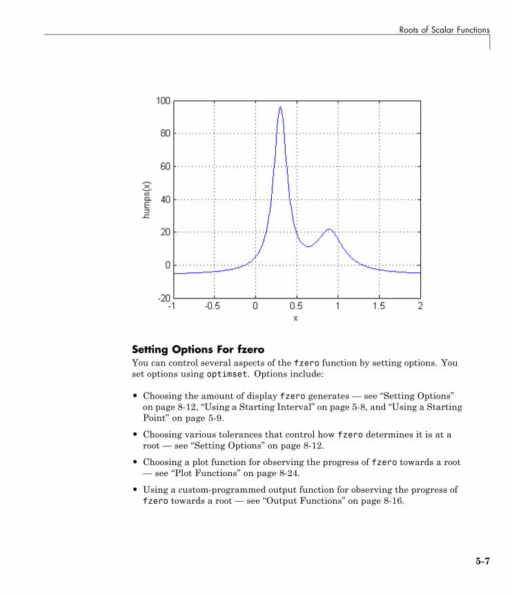
Roots of Scalar Functions
Setting Options For fzeroYou can control several aspects of the fzero function by setting options. Youset options using optimset. Options include:
• Choosing the amount of display fzero generates — see “Setting Options”on page 8-12, “Using a Starting Interval” on page 5-8, and “Using a StartingPoint” on page 5-9.
• Choosing various tolerances that control how fzero determines it is at aroot — see “Setting Options” on page 8-12.
• Choosing a plot function for observing the progress of fzero towards a root— see “Plot Functions” on page 8-24.
• Using a custom-programmed output function for observing the progress offzero towards a root — see “Output Functions” on page 8-16.
5-7
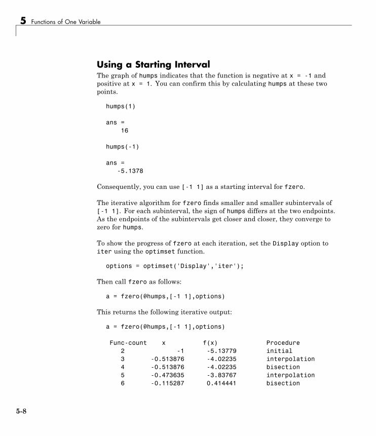
5 Functions of One Variable
Using a Starting IntervalThe graph of humps indicates that the function is negative at x = -1 andpositive at x = 1. You can confirm this by calculating humps at these twopoints.
humps(1)
ans =16
humps(-1)
ans =-5.1378
Consequently, you can use [-1 1] as a starting interval for fzero.
The iterative algorithm for fzero finds smaller and smaller subintervals of[-1 1]. For each subinterval, the sign of humps differs at the two endpoints.As the endpoints of the subintervals get closer and closer, they converge tozero for humps.
To show the progress of fzero at each iteration, set the Display option toiter using the optimset function.
options = optimset('Display','iter');
Then call fzero as follows:
a = fzero(@humps,[-1 1],options)
This returns the following iterative output:
a = fzero(@humps,[-1 1],options)
Func-count x f(x) Procedure2 -1 -5.13779 initial3 -0.513876 -4.02235 interpolation4 -0.513876 -4.02235 bisection5 -0.473635 -3.83767 interpolation6 -0.115287 0.414441 bisection
5-8
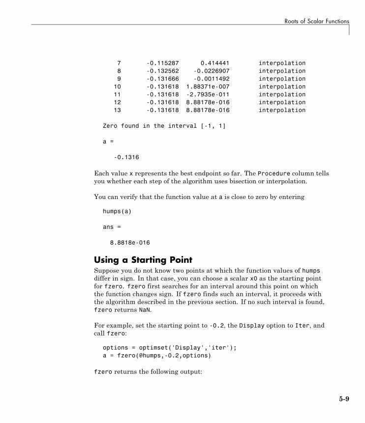
Roots of Scalar Functions
7 -0.115287 0.414441 interpolation8 -0.132562 -0.0226907 interpolation9 -0.131666 -0.0011492 interpolation
10 -0.131618 1.88371e-007 interpolation11 -0.131618 -2.7935e-011 interpolation12 -0.131618 8.88178e-016 interpolation13 -0.131618 8.88178e-016 interpolation
Zero found in the interval [-1, 1]
a =
-0.1316
Each value x represents the best endpoint so far. The Procedure column tellsyou whether each step of the algorithm uses bisection or interpolation.
You can verify that the function value at a is close to zero by entering
humps(a)
ans =
8.8818e-016
Using a Starting PointSuppose you do not know two points at which the function values of humpsdiffer in sign. In that case, you can choose a scalar x0 as the starting pointfor fzero. fzero first searches for an interval around this point on whichthe function changes sign. If fzero finds such an interval, it proceeds withthe algorithm described in the previous section. If no such interval is found,fzero returns NaN.
For example, set the starting point to -0.2, the Display option to Iter, andcall fzero:
options = optimset('Display','iter');a = fzero(@humps,-0.2,options)
fzero returns the following output:
5-9
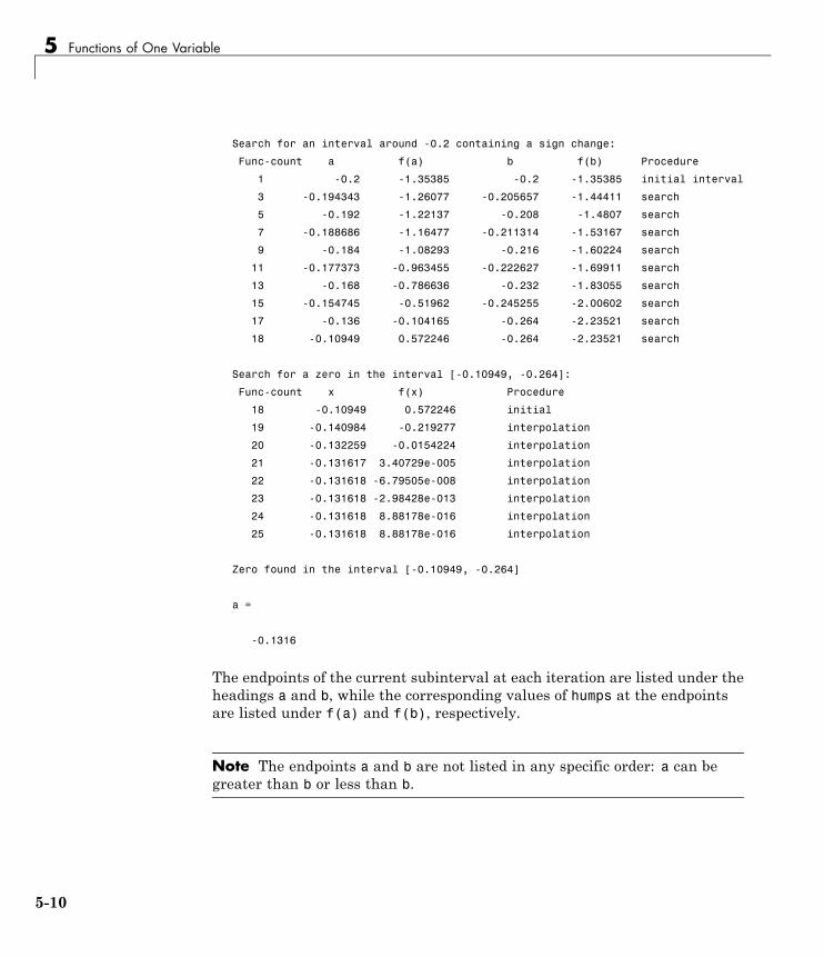
5 Functions of One Variable
Search for an interval around -0.2 containing a sign change:
Func-count a f(a) b f(b) Procedure
1 -0.2 -1.35385 -0.2 -1.35385 initial interval
3 -0.194343 -1.26077 -0.205657 -1.44411 search
5 -0.192 -1.22137 -0.208 -1.4807 search
7 -0.188686 -1.16477 -0.211314 -1.53167 search
9 -0.184 -1.08293 -0.216 -1.60224 search
11 -0.177373 -0.963455 -0.222627 -1.69911 search
13 -0.168 -0.786636 -0.232 -1.83055 search
15 -0.154745 -0.51962 -0.245255 -2.00602 search
17 -0.136 -0.104165 -0.264 -2.23521 search
18 -0.10949 0.572246 -0.264 -2.23521 search
Search for a zero in the interval [-0.10949, -0.264]:
Func-count x f(x) Procedure
18 -0.10949 0.572246 initial
19 -0.140984 -0.219277 interpolation
20 -0.132259 -0.0154224 interpolation
21 -0.131617 3.40729e-005 interpolation
22 -0.131618 -6.79505e-008 interpolation
23 -0.131618 -2.98428e-013 interpolation
24 -0.131618 8.88178e-016 interpolation
25 -0.131618 8.88178e-016 interpolation
Zero found in the interval [-0.10949, -0.264]
a =
-0.1316
The endpoints of the current subinterval at each iteration are listed under theheadings a and b, while the corresponding values of humps at the endpointsare listed under f(a) and f(b), respectively.
Note The endpoints a and b are not listed in any specific order: a can begreater than b or less than b.
5-10
Roots of Scalar Functions
For the first nine steps, the sign of humps is negative at both endpoints ofthe current subinterval, which is shown in the output. At the tenth step,the sign of humps is positive at the endpoint, -0.10949, but negative at theendpoint, -0.264. From this point on, the algorithm continues to narrowdown the interval [-0.10949 -0.264], as described in the previous section,until it reaches the value -0.1316.
5-11

5 Functions of One Variable
DerivativesThe polyder function computes the derivative of any polynomial. To obtainthe derivative of the polynomial p = [1 0 -2 -5],
q = polyder(p)
q =3 0 -2
polyder also computes the derivative of the product or quotient of twopolynomials. For example, create two polynomials a and b:
a = [1 3 5];b = [2 4 6];
Calculate the derivative of the product a*b by calling polyder with a singleoutput argument:
c = polyder(a,b)
c =8 30 56 38
Calculate the derivative of the quotient a/b by calling polyder with twooutput arguments:
[q,d] = polyder(a,b)
q =-2 -8 -2
d =4 16 40 48 36
q/d is the result of the operation.
5-12

Convolution
ConvolutionPolynomial multiplication and division correspond to the operationsconvolution and deconvolution. The functions conv and deconv implementthese operations.
Consider the polynomials and . Tocompute their product,
a = [1 2 3]; b = [4 5 6];c = conv(a,b)
c =4 13 28 27 18
Use deconvolution to divide back out of the product:
[q,r] = deconv(c,a)
q =4 5 6
r =0 0 0 0 0
5-13
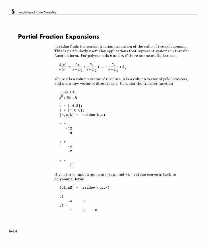
5 Functions of One Variable
Partial Fraction Expansionsresidue finds the partial fraction expansion of the ratio of two polynomials.This is particularly useful for applications that represent systems in transferfunction form. For polynomials b and a, if there are no multiple roots,
where r is a column vector of residues, p is a column vector of pole locations,and k is a row vector of direct terms. Consider the transfer function
b = [-4 8];a = [1 6 8];[r,p,k] = residue(b,a)
r =-12
8
p =-4-2
k =[]
Given three input arguments (r, p, and k), residue converts back topolynomial form:
[b2,a2] = residue(r,p,k)
b2 =-4 8
a2 =1 6 8
5-14
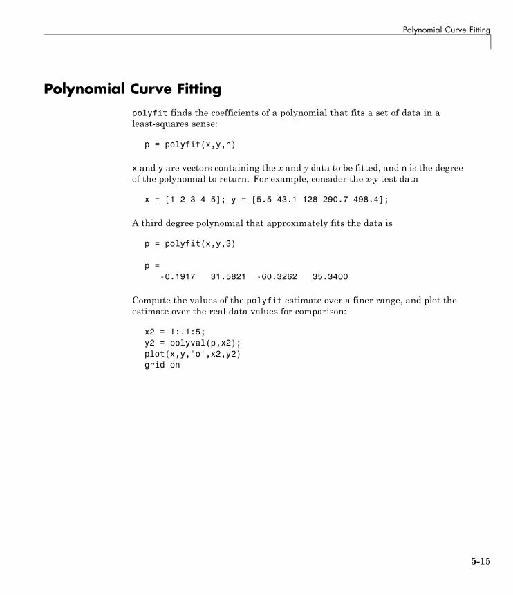
Polynomial Curve Fitting
Polynomial Curve Fittingpolyfit finds the coefficients of a polynomial that fits a set of data in aleast-squares sense:
p = polyfit(x,y,n)
x and y are vectors containing the x and y data to be fitted, and n is the degreeof the polynomial to return. For example, consider the x-y test data
x = [1 2 3 4 5]; y = [5.5 43.1 128 290.7 498.4];
A third degree polynomial that approximately fits the data is
p = polyfit(x,y,3)
p =-0.1917 31.5821 -60.3262 35.3400
Compute the values of the polyfit estimate over a finer range, and plot theestimate over the real data values for comparison:
x2 = 1:.1:5;y2 = polyval(p,x2);plot(x,y,'o',x2,y2)grid on
5-15
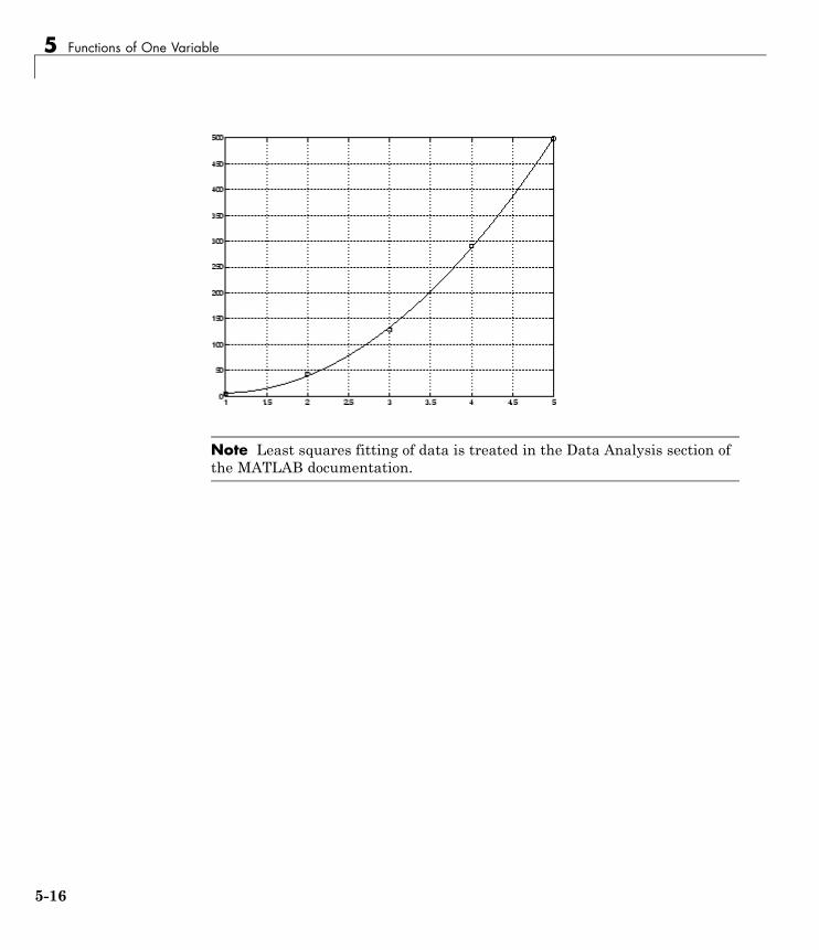
5 Functions of One Variable
Note Least squares fitting of data is treated in the Data Analysis section ofthe MATLAB documentation.
5-16
Characteristic Polynomials
Characteristic PolynomialsThe poly function also computes the coefficients of the characteristicpolynomial of a matrix:
A = [1.2 3 -0.9; 5 1.75 6; 9 0 1];poly(A)
ans =1.0000 -3.9500 -1.8500 -163.2750
The roots of this polynomial, computed with roots, are the characteristicroots, or eigenvalues, of the matrix A. (Use eig to compute the eigenvaluesof a matrix directly.)
5-17

5 Functions of One Variable
5-18

6
Computational Geometry
• “Overview” on page 6-2
• “Triangulation Representations” on page 6-3
• “Delaunay Triangulation” on page 6-17
• “Spatial Searching” on page 6-47
• “Voronoi Diagrams” on page 6-57
• “Convex Hulls” on page 6-66
6 Computational Geometry
OverviewMATLAB software provides a variety of tools to solve problems thatare geometric in nature. These problems encompass simple geometricqueries such as point-in-polygon tests, to more complex problems such asnearest-neighbor queries. Convex hulls, Delaunay triangulations, andVoronoi diagrams are examples of fundamental geometric algorithms thatMATLAB provides. These algorithms have many practical uses in thescientific development.
MATLAB provides both function-based and class-based tools for computationalgeometry. The function-based tools are convenient when the output from thefunction is sufficiently complete to get you to the solution. The class-basedtools are more versatile because they provide complementary methods thatare often needed to work with the resulting data. A function typically takesinput, performs some computation, and outputs the result in matrix format.
In contrast, a class may take input, perform some computation, cachethe result and provide methods that allow you to query and work withthe result more efficiently. For example, the delaunay function creates atriangulation from a set of points and returns the triangulation in an array.The DelaunayTri class also triangulates a set of points. In addition, it allowsyou to modify the triangulation and it provides methods for finding nearestneighbors and traversing the triangulation data structure, etc. These methodsare very efficient because the class holds the triangulation in memory.
6-2

Triangulation Representations
Triangulation Representations
2-D and 3-D DomainsTriangulations are often used to represent 2-D and 3-D geometric domains inapplication areas such as computer graphics, physical modeling, geographicinformation systems, medical imaging, and more. The map polygon shownhere
can be represented by the triangulation on the map shown here
6-3
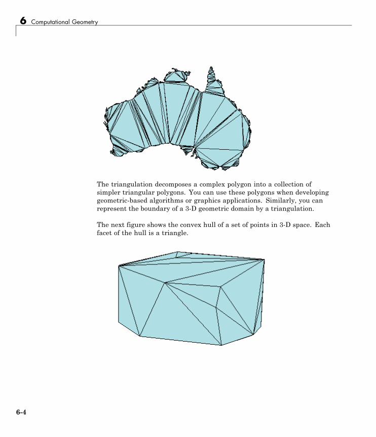
6 Computational Geometry
The triangulation decomposes a complex polygon into a collection ofsimpler triangular polygons. You can use these polygons when developinggeometric-based algorithms or graphics applications. Similarly, you canrepresent the boundary of a 3-D geometric domain by a triangulation.
The next figure shows the convex hull of a set of points in 3-D space. Eachfacet of the hull is a triangle.
6-4
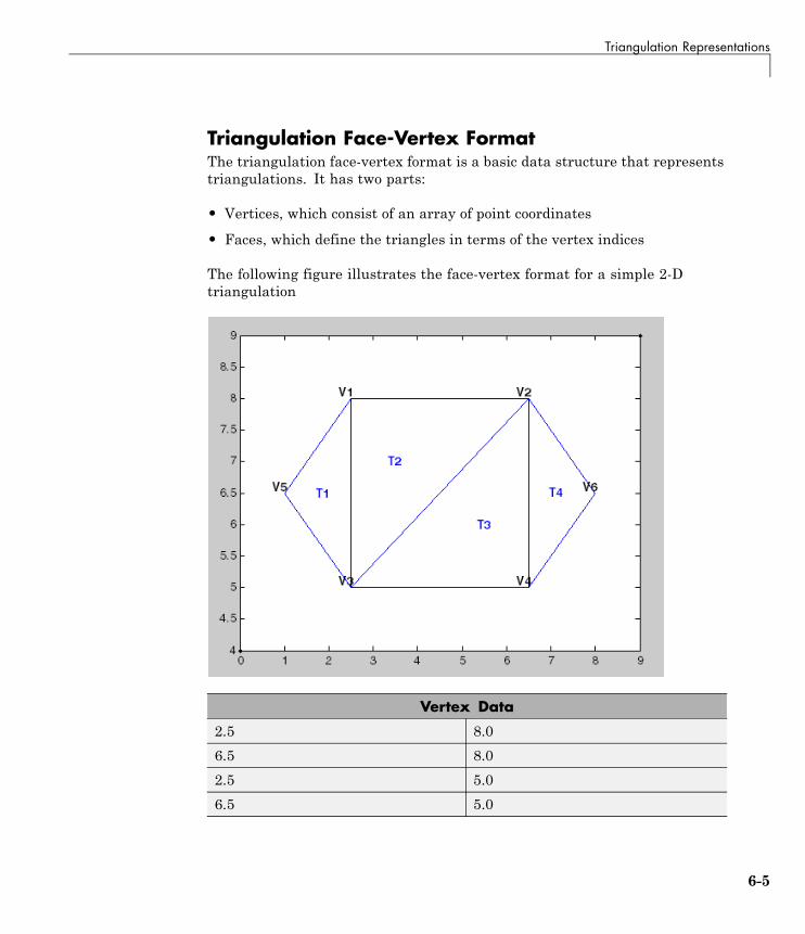
Triangulation Representations
Triangulation Face-Vertex FormatThe triangulation face-vertex format is a basic data structure that representstriangulations. It has two parts:
• Vertices, which consist of an array of point coordinates
• Faces, which define the triangles in terms of the vertex indices
The following figure illustrates the face-vertex format for a simple 2-Dtriangulation
Vertex Data
2.5 8.0
6.5 8.0
2.5 5.0
6.5 5.0
6-5
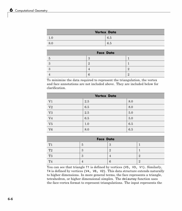
6 Computational Geometry
Vertex Data
1.0 6.5
8.0 6.5
Face Data
5 3 1
3 2 1
3 4 2
4 6 2
To minimize the data required to represent the triangulation, the vertexand face annotations are not included above. They are included below forclarification.
Vertex Data
V1 2.5 8.0
V2 6.5 8.0
V3 2.5 5.0
V4 6.5 5.0
V5 1.0 6.5
V6 8.0 6.5
Face Data
T1 5 3 1
T2 3 2 1
T3 3 4 2
T4 4 6 2
You can see that triangle T1 is defined by vertices {V5, V3, V1}. Similarly,T4 is defined by vertices {V4, V6, V2}. This data structure extends naturallyto higher dimensions. In more general terms, the face represents a triangle,tetrahedron, or higher dimensional simplex. The delaunay function usesthe face-vertex format to represent triangulations. The input represents the
6-6
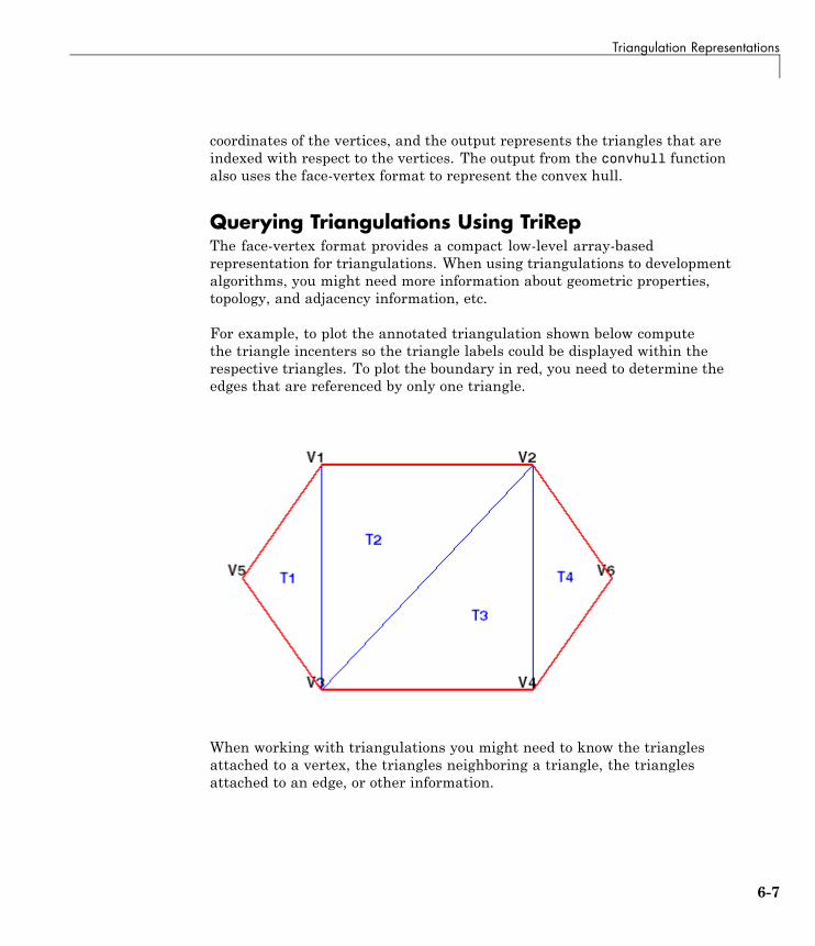
Triangulation Representations
coordinates of the vertices, and the output represents the triangles that areindexed with respect to the vertices. The output from the convhull functionalso uses the face-vertex format to represent the convex hull.
Querying Triangulations Using TriRepThe face-vertex format provides a compact low-level array-basedrepresentation for triangulations. When using triangulations to developmentalgorithms, you might need more information about geometric properties,topology, and adjacency information, etc.
For example, to plot the annotated triangulation shown below computethe triangle incenters so the triangle labels could be displayed within therespective triangles. To plot the boundary in red, you need to determine theedges that are referenced by only one triangle.
When working with triangulations you might need to know the trianglesattached to a vertex, the triangles neighboring a triangle, the trianglesattached to an edge, or other information.
6-7

6 Computational Geometry
The TriRep ClassMATLAB provides a TriRep class that allows you to query triangulations in anefficient manner. TriRep is an abbreviation for Triangulation Representation.It supports 2-D and 3-D triangulations composed of triangles, and 3-Dtriangulations composed of tetrahedra. It lets you represent triangulationsyou imported into MATLAB or created directly in MATLAB using thecomputational geometry tools. The TriRep class supports many geometricand topological queries that simplify the development of triangulation-basedalgorithms.
Note that TriRep does not create triangulations. Use TriRep to representtriangulations that you import into MATLAB or create using one of thecomputational geometry tools.
Create a TriRep in one of two ways:
• You can create a TriRep from face-vertex data. This data may be theoutput from a MATLAB function such as delaunay or a 3-D convex hullcomputation using convhull. You also can import face-vertex data thatwas created by another application outside of MATLAB. When workingwith imported data you should ensure the face data uses 1-based indexingto refer to the vertex array as opposed to 0-based indexing.
• MATLAB creates a TriRep when you create a Delaunay triangulationusing the DelaunayTri class. That’s because a Delaunay triangulation(DelaunayTri) is a triangulation representation (TriRep). This doesn’tmean they are identical; the DelaunayTri class has additional function-likemethods specific to Delaunay triangulations. If you view TriRep as aset of triangulations, you could say the DelaunayTri is a subset. It’s aspecific type of triangulation. In more formal MATLAB language terms,DelaunayTri is a subclass of TriRep.
Creating a TriRep from Face-Vertex Data. You can use the triangulationface-vertex data from the previous section to create a TriRep explore what itis, and what it can do.
Create a matrix x that represents the vertex data:
x = [ 2.5 8.06.5 8.0
6-8
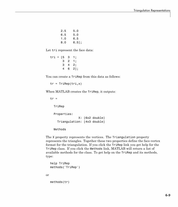
Triangulation Representations
2.5 5.06.5 5.01.0 6.58.0 6.5];
Let tri represent the face data:
tri = [5 3 1;3 2 1;3 4 2;4 6 2];
You can create a TriRep from this data as follows:
tr = TriRep(tri,x)
When MATLAB creates the TriRep, it outputs:
tr =
TriRep
Properties:X: [6x2 double]
Triangulation: [4x3 double]
Methods
The X property represents the vertices. The Triangulation propertyrepresents the triangles. Together these two properties define the face-vertexformat for the triangulation. If you click the TriRep link you get help for theTriRep class. If you click the Methods link, MATLAB will return a list ofavailable methods for the class. To get help on the TriRep and its methods,type:
help TriRepmethods('TriRep')
or
methods(tr)
6-9
6 Computational Geometry
The TriRep class is a wrapper around the face-vertex format. The real benefitis the useful methods that TriRep provides. The methods are like functionsthat a TriRep object can call.
You can access the properties in a TriRep in the same way as you wouldfor a Struct.
tr.X
returns the vertex data.
tr.Triangulation
returns the Triangulation data.
TriRep provides a shorthand way to index into the Triangulation propertymatrix. To access the first triangle in the triangulation, type:
tr.Triangulation(1, :)
The shorthand way of getting the first triangle is:
tr(1, :)
Likewise, you can get the first vertex of the first triangle:
tr(1, 1)
Or the second vertex of the first triangle:
tr(1, 2)
Or you can get all the triangles in the triangulation:
tr(:, :)
You can use triplot to plot the TriRep. While it’s not a method of the class,triplot knows what a TriRep is and how to plot it.
triplot(tr);axis equal
6-10
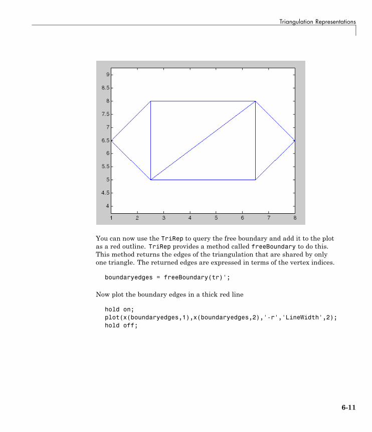
Triangulation Representations
You can now use the TriRep to query the free boundary and add it to the plotas a red outline. TriRep provides a method called freeBoundary to do this.This method returns the edges of the triangulation that are shared by onlyone triangle. The returned edges are expressed in terms of the vertex indices.
boundaryedges = freeBoundary(tr)';
Now plot the boundary edges in a thick red line
hold on;plot(x(boundaryedges,1),x(boundaryedges,2),'-r','LineWidth',2);hold off;
6-11
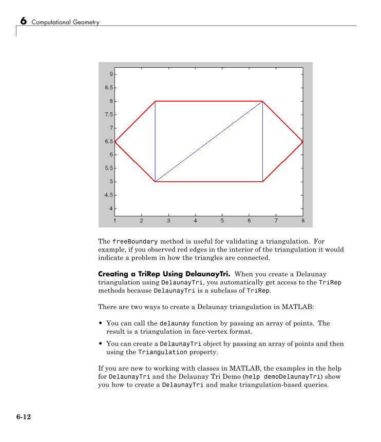
6 Computational Geometry
The freeBoundary method is useful for validating a triangulation. Forexample, if you observed red edges in the interior of the triangulation it wouldindicate a problem in how the triangles are connected.
Creating a TriRep Using DelaunayTri. When you create a Delaunaytriangulation using DelaunayTri, you automatically get access to the TriRepmethods because DelaunayTri is a subclass of TriRep.
There are two ways to create a Delaunay triangulation in MATLAB:
• You can call the delaunay function by passing an array of points. Theresult is a triangulation in face-vertex format.
• You can create a DelaunayTri object by passing an array of points and thenusing the Triangulation property.
If you are new to working with classes in MATLAB, the examples in the helpfor DelaunayTri and the Delaunay Tri Demo (help demoDelaunayTri) showyou how to create a DelaunayTri and make triangulation-based queries.
6-12

Triangulation Representations
The documentation on DelaunayTri also provides introductory material andexamples.
You can create a simple Delaunay triangulation using DelaunayTri,and then query this triangulation using one of the methods provided bythe parent class, TriRep. This example uses the point data set from theprevious example. In this instance, DelaunayTri automatically generatesthe triangulation from the point set.
Create a set of points:
x = [ 2.5 8.06.5 8.02.5 5.06.5 5.01.0 6.58.0 6.5];
Create a DelaunayTri from the set of points:
dt = DelaunayTri(x)
When MATLAB creates the DelaunayTri, it outputs:
dt =
DelaunayTri
Properties:X: [6x2 double]
Triangulation: [4x3 double]
Methods
DelaunayTri has properties X and Triangulation like TriRep.Triangulation is the Delaunay triangulation MATLAB creates. Just likeTriRep, the triangulation is in face-vertex format.
Access the triangulation using direct indexing, just like TriRep:
6-13
6 Computational Geometry
dt(1, :) % Returns the 1st triangledt(:, :) % Returns the Triangulation data
Use the triplot function to plot the triangulation:
triplot(dt)axis equal
The parent class, TriRep, provides the incentersmethod to compute theincenters of the triangles in the triangulation. incenters is a method ofTriRep because computing incenters is not specific to Delaunay triangulations.It’s something you would like to be able to do for any general triangulationand that’s what a TriRep is. Call the incenters method as follows:
ic = incenters(dt)ic =
1.8787 6.50003.5000 7.00005.5000 6.00007.1213 6.5000
The returned value, ic, is an array of coordinates representing the incentersof the triangles.
Add text to the plot to place the labels within the triangles. Use the incentersto locate the text.
hold onnumtri = size(dt,1);trilabels = arrayfun(@(x) {sprintf('T%d', x)}, (1:numtri)');Htl = text(ic(:,1), ic(:,2), trilabels,'FontWeight','bold', ...'HorizontalAlignment', 'center', 'Color', 'blue');hold off
Instead of creating a Delaunay triangulation using DelaunayTri, you coulduse the delaunay function create the triangulation in face-vertex format, andthen create a TriRep from that. For example you could do the following:
X = [ 2.5 8.06.5 8.0
6-14
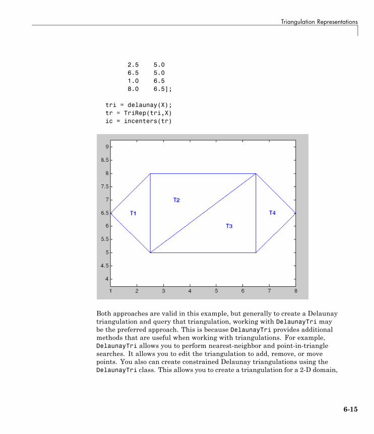
Triangulation Representations
2.5 5.06.5 5.01.0 6.58.0 6.5];
tri = delaunay(X);tr = TriRep(tri,X)ic = incenters(tr)
Both approaches are valid in this example, but generally to create a Delaunaytriangulation and query that triangulation, working with DelaunayTri maybe the preferred approach. This is because DelaunayTri provides additionalmethods that are useful when working with triangulations. For example,DelaunayTri allows you to perform nearest-neighbor and point-in-trianglesearches. It allows you to edit the triangulation to add, remove, or movepoints. You also can create constrained Delaunay triangulations using theDelaunayTri class. This allows you to create a triangulation for a 2-D domain,
6-15
6 Computational Geometry
such as the map polygon illustrated in “Triangulation Representations” onpage 6-3.
“Delaunay Triangulation” on page 6-17 provides you with more informationand examples on how to create, query, and work with DelaunayTri.“Spatial Searching” on page 6-47 provides further information on searchingtriangulations including non-Delaunay triangulations.
6-16
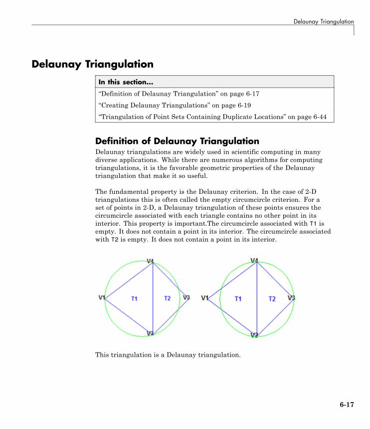
Delaunay Triangulation
Delaunay Triangulation
In this section...
“Definition of Delaunay Triangulation” on page 6-17
“Creating Delaunay Triangulations” on page 6-19
“Triangulation of Point Sets Containing Duplicate Locations” on page 6-44
Definition of Delaunay TriangulationDelaunay triangulations are widely used in scientific computing in manydiverse applications. While there are numerous algorithms for computingtriangulations, it is the favorable geometric properties of the Delaunaytriangulation that make it so useful.
The fundamental property is the Delaunay criterion. In the case of 2-Dtriangulations this is often called the empty circumcircle criterion. For aset of points in 2-D, a Delaunay triangulation of these points ensures thecircumcircle associated with each triangle contains no other point in itsinterior. This property is important.The circumcircle associated with T1 isempty. It does not contain a point in its interior. The circumcircle associatedwith T2 is empty. It does not contain a point in its interior.
This triangulation is a Delaunay triangulation.
6-17

6 Computational Geometry
By contrast: The circumcircle associated with T1 is not empty; it contains V3in its interior. The circumcircle associated with T2 is not empty; it containsV1 in its interior.
This triangulation is not a Delaunay triangulation.
Delaunay triangles are said to be “well shaped” because in fulfilling theempty circumcircle property, triangles with large internal angles are selectedover ones with small internal angles. The triangles in the non-Delaunaytriangulation have sharp angles at vertices V2 and V4. If the edge {V2, V4}were replaced by an edge joining V1 and V3, the minimum angle would bemaximized and the triangulation would become a Delaunay triangulation.Also, the Delaunay triangulation connects points in a nearest-neighbormanner. These two characteristics, well-shaped triangles and thenearest-neighbor relation, have important implications in practice andmotivate the use of Delaunay triangulations in scattered data interpolation.
While the Delaunay property is well defined, the topology of the triangulationis not unique in the presence of degenerate point sets. In two dimensions,degeneracies arise when four or more unique points lie on the same circle. Thevertices of a square, for example, have a nonunique Delaunay triangulation.
6-18
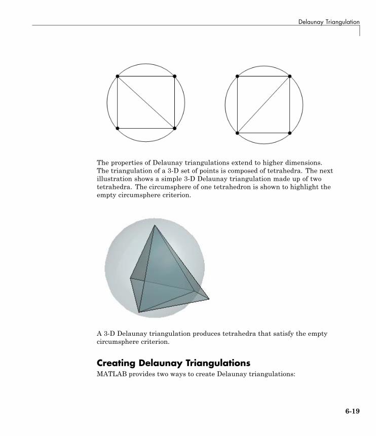
Delaunay Triangulation
The properties of Delaunay triangulations extend to higher dimensions.The triangulation of a 3-D set of points is composed of tetrahedra. The nextillustration shows a simple 3-D Delaunay triangulation made up of twotetrahedra. The circumsphere of one tetrahedron is shown to highlight theempty circumsphere criterion.
A 3-D Delaunay triangulation produces tetrahedra that satisfy the emptycircumsphere criterion.
Creating Delaunay TriangulationsMATLAB provides two ways to create Delaunay triangulations:
6-19
6 Computational Geometry
• The functions delaunay and delaunayn
• The DelaunayTri class
The delaunay function supports the creation of 2-D and 3-D Delaunaytriangulations. The delaunayn function supports creating Delaunaytriangulations in 4-D and higher.
Tip Creating Delaunay triangulations in dimensions higher than 6-D isgenerally not practical for moderate to large point sets due to the exponentialgrowth in required memory.
The DelaunayTri class supports creating Delaunay triangulations in2-D and 3-D. It provides many methods that are useful for developingtriangulation-based algorithms. These class methods are like functions, butthey are restricted to work with triangulations created using DelaunayTri.The DelaunayTri class also supports the creation of related constructs suchas the convex hull and Voronoi diagram. It also supports the creation ofconstrained Delaunay triangulations.
In summary:
• The delaunay function is useful when you only require the basictriangulation data, and that data is sufficiently complete for the applicationat hand.
• The DelaunayTri class is useful when you require the triangulation and inaddition you want to perform any of these operations:
- Search the triangulation for triangles/tetrahedral enclosing a querypoint.
- Use the triangulation to perform a nearest-neighbor point search.
- Query the triangulation’s topological adjacency or geometric properties.
- Modify the triangulation to insert or remove points.
- Constrain edges in the triangulation—this is called a constrainedDelaunay triangulation.
6-20
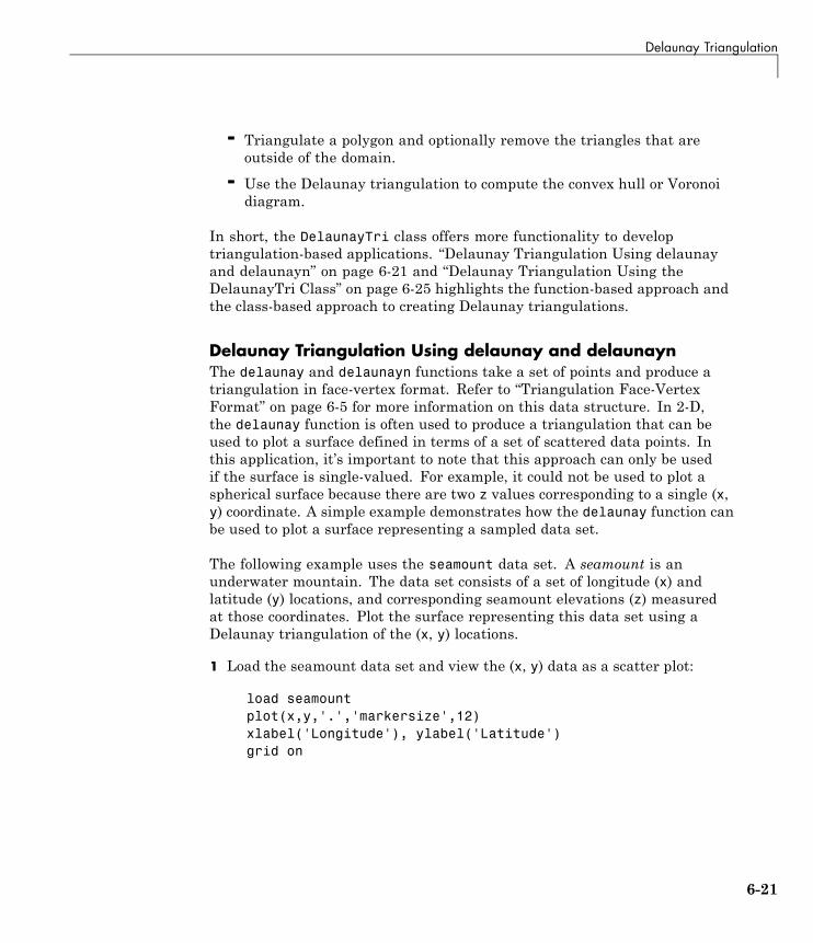
Delaunay Triangulation
- Triangulate a polygon and optionally remove the triangles that areoutside of the domain.
- Use the Delaunay triangulation to compute the convex hull or Voronoidiagram.
In short, the DelaunayTri class offers more functionality to developtriangulation-based applications. “Delaunay Triangulation Using delaunayand delaunayn” on page 6-21 and “Delaunay Triangulation Using theDelaunayTri Class” on page 6-25 highlights the function-based approach andthe class-based approach to creating Delaunay triangulations.
Delaunay Triangulation Using delaunay and delaunaynThe delaunay and delaunayn functions take a set of points and produce atriangulation in face-vertex format. Refer to “Triangulation Face-VertexFormat” on page 6-5 for more information on this data structure. In 2-D,the delaunay function is often used to produce a triangulation that can beused to plot a surface defined in terms of a set of scattered data points. Inthis application, it’s important to note that this approach can only be usedif the surface is single-valued. For example, it could not be used to plot aspherical surface because there are two z values corresponding to a single (x,y) coordinate. A simple example demonstrates how the delaunay function canbe used to plot a surface representing a sampled data set.
The following example uses the seamount data set. A seamount is anunderwater mountain. The data set consists of a set of longitude (x) andlatitude (y) locations, and corresponding seamount elevations (z) measuredat those coordinates. Plot the surface representing this data set using aDelaunay triangulation of the (x, y) locations.
1 Load the seamount data set and view the (x, y) data as a scatter plot:
load seamountplot(x,y,'.','markersize',12)xlabel('Longitude'), ylabel('Latitude')grid on
6-21
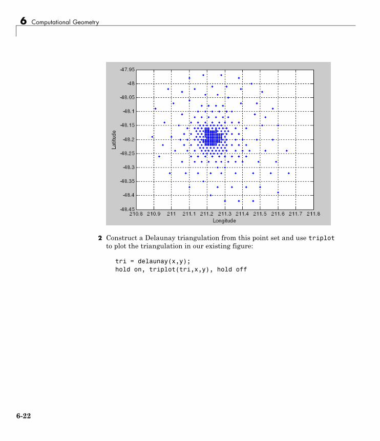
6 Computational Geometry
2 Construct a Delaunay triangulation from this point set and use triplotto plot the triangulation in our existing figure:
tri = delaunay(x,y);hold on, triplot(tri,x,y), hold off
6-22
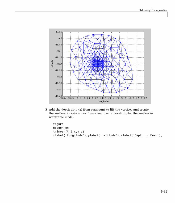
Delaunay Triangulation
3 Add the depth data (z) from seamount to lift the vertices and createthe surface. Create a new figure and use trimesh to plot the surface inwireframe mode:
figurehidden ontrimesh(tri,x,y,z)xlabel('Longitude'),ylabel('Latitude'),zlabel('Depth in Feet');
6-23
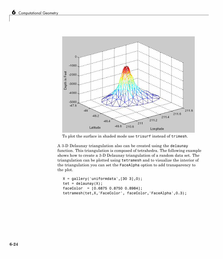
6 Computational Geometry
To plot the surface in shaded mode use trisurf instead of trimesh.
A 3-D Delaunay triangulation also can be created using the delaunayfunction. This triangulation is composed of tetrahedra. The following exampleshows how to create a 3-D Delaunay triangulation of a random data set. Thetriangulation can be plotted using tetramesh and to visualize the interior ofthe triangulation you can set the FaceAlpha option to add transparency tothe plot.
X = gallery('uniformdata',[30 3],0);tet = delaunay(X);faceColor = [0.6875 0.8750 0.8984];tetramesh(tet,X,'FaceColor', faceColor,'FaceAlpha',0.3);
6-24
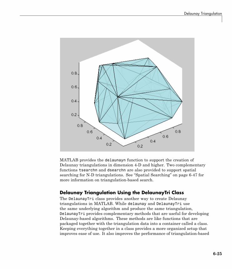
Delaunay Triangulation
MATLAB provides the delaunayn function to support the creation ofDelaunay triangulations in dimension 4-D and higher. Two complementaryfunctions tsearchn and dsearchn are also provided to support spatialsearching for N-D triangulations. See “Spatial Searching” on page 6-47 formore information on triangulation-based search.
Delaunay Triangulation Using the DelaunayTri ClassThe DelaunayTri class provides another way to create Delaunaytriangulations in MATLAB. While delaunay and DelaunayTri usethe same underlying algorithm and produce the same triangulation,DelaunayTri provides complementary methods that are useful for developingDelaunay-based algorithms. These methods are like functions that arepackaged together with the triangulation data into a container called a class.Keeping everything together in a class provides a more organized setup thatimproves ease of use. It also improves the performance of triangulation-based
6-25
6 Computational Geometry
searches such as point location and nearest neighbor. DelaunayTri supportsincremental editing of the Delaunay triangulation. You can also impose edgeconstraints in 2-D.
“Triangulation Representations” on page 6-3 presents the class TriRep thatrepresents triangulations. In addition, TriRep provides many methods thatallow you to make topological and geometric queries. DelaunayTri alsorepresents a triangulation and in fact, represents it in terms of a TriRep. Youcan view DelaunayTri as a subset of TriRep, (in MATLAB language terms,DelaunayTri is a subclass of TriRep). This simply means that a DelaunayTri(Delaunay triangulation) is a TriRep (triangulation representation) that hassomething extra. In this instance the difference is the Delaunay criterion thatthe triangulation satisfies and the extra methods that DelaunayTri providesthat are unique to Delaunay triangulations.
These distinctions will become clearer with examples. The next exampleuses the seamount data to explore how you can create, query, and edit aDelaunay triangulation with DelaunayTri. The seamount data set contains(x, y) locations and corresponding elevations (z) that define the surface ofthe seamount.
Load and triangulate the (x, y) data:
load seamountdt = DelaunayTri(x,y)
MATLAB outputs the following when it creates the DelaunayTri:
dt =
DelaunayTri
Properties:Constraints: []
X: [294x2 double]Triangulation: [566x3 double]
Methods, Superclasses
6-26
Delaunay Triangulation
The Constraints property is empty because you have not imposed edgeconstraints (see “Constrained Delaunay Triangulation” on page 6-37for more information about constraints). The X property represents thecoordinates of the vertices, and the Triangulation property represents thetriangles. Together these two properties define the face-vertex format for thetriangulation. If you click on the DelaunayTri link you will get help for theDelaunayTri class, and if you click on the Methods link, MATLAB will returna list of available methods for the class. You can also type the following to gethelp on the DelaunayTri class and see its list of methods:
help DelaunayTrimethods('DelaunayTri')
Or
methods(dt);
The Superclasses link provides help for TriRep, the superclass forDelaunayTri. As in the case of TriRep, the DelaunayTri class is a wrapperaround the face-vertex format together with a set of complementary methods.Similarly, you can access the properties in a DelaunayTri in the same wayas you would for a Struct.
To access the vertex data:
dt.X
To access the triangulation:
dt.Triangulation
To access the first triangle in the Triangulation property:
dt.Triangulation(1, :)
DelaunayTri provides a shorthand way of indexing into the Triangulationproperty matrix. The shorthand way to get the first triangle is:
dt(1, :)
You can get the first vertex of the first triangle:
6-27
6 Computational Geometry
dt(1, 1)
Or the second vertex of the first triangle:
dt(1, 2)
Or get all the triangles in the triangulation:
dt(:, :)
Indexing into the DelaunayTri output dt works like indexing into atriangulation the output from delaunay. The difference between the twoare the extra methods that you can call on dt. You can use triplot to plotthe DelaunayTri; while it’s not a method of the class, triplot recognizes aDelaunayTri and knows how to plot it.
triplot(dt);axis equalxlabel('Longitude'), ylabel('Latitude')grid on
You could use
triplot(dt(:,:), dt.X(:,1), dt.X(:,2));
to get the same plot.
6-28
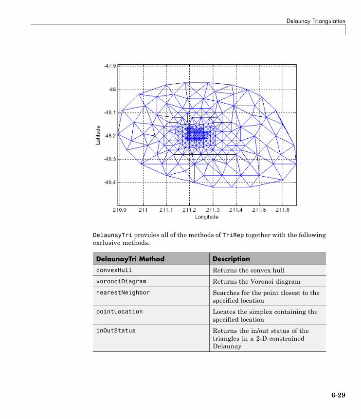
Delaunay Triangulation
DelaunayTri provides all of the methods of TriRep together with the followingexclusive methods.
DelaunayTri Method Description
convexHull Returns the convex hull
voronoiDiagram Returns the Voronoi diagram
nearestNeighbor Searches for the point closest to thespecified location
pointLocation Locates the simplex containing thespecified location
inOutStatus Returns the in/out status of thetriangles in a 2-D constrainedDelaunay
6-29
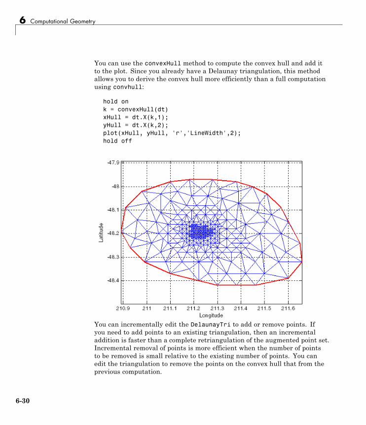
6 Computational Geometry
You can use the convexHull method to compute the convex hull and add itto the plot. Since you already have a Delaunay triangulation, this methodallows you to derive the convex hull more efficiently than a full computationusing convhull:
hold onk = convexHull(dt)xHull = dt.X(k,1);yHull = dt.X(k,2);plot(xHull, yHull, 'r','LineWidth',2);hold off
You can incrementally edit the DelaunayTri to add or remove points. Ifyou need to add points to an existing triangulation, then an incrementaladdition is faster than a complete retriangulation of the augmented point set.Incremental removal of points is more efficient when the number of pointsto be removed is small relative to the existing number of points. You canedit the triangulation to remove the points on the convex hull that from theprevious computation.
6-30

Delaunay Triangulation
% Plot the result in a new figurefigureplot(xHull, yHull, 'r','LineWidth',2);axis equalxlabel('Longitude'), ylabel('Latitude')grid on
% The convex hull topology duplicates the start% and end vertex. To remove the duplicate entry:k(end) = [];
% Now remove the points on the convex hulldt.X(k,:) = []% Plot the new triangulationhold ontriplot(dt);hold off
6-31
6 Computational Geometry
There is one vertex that is just inside the boundary of the convex hull thatwas not removed. The fact that it’s interior to the hull can be seen using theZoom-In tool in the figure. You could plot the vertex labels to determine theindex of this vertex and remove it from the triangulation. You can also usethe nearestNeighbor method to identify the index more readily.
% The point is close to location (211.6, -48.15)% Use the nearestNeighbor method to find the nearest vertexvertexId = nearestNeighbor(dt, 211.6, -48.15)
% Now remove that vertex from the triangulationdt.X(vertexId,:) = []
% Plot the new triangulationfigureplot(xHull, yHull, 'r','LineWidth',2);axis equalxlabel('Longitude'), ylabel('Latitude')grid onhold ontriplot(dt);hold off
6-32

Delaunay Triangulation
Add points to the existing triangulation as follows:
% Add 4 points to form a rectangle around the triangulationXadditional = [210.9 -48.5; 211.6 -48.5; ...
211.6 -47.9; 210.9 -47.9];dt.X(end+(1:4),:) = Xadditional
% Close all existing figuresclose all
% Plot the new triangulationfigureplot(xHull, yHull, 'r','LineWidth',2);axis equalxlabel('Longitude'), ylabel('Latitude')grid onhold on
6-33
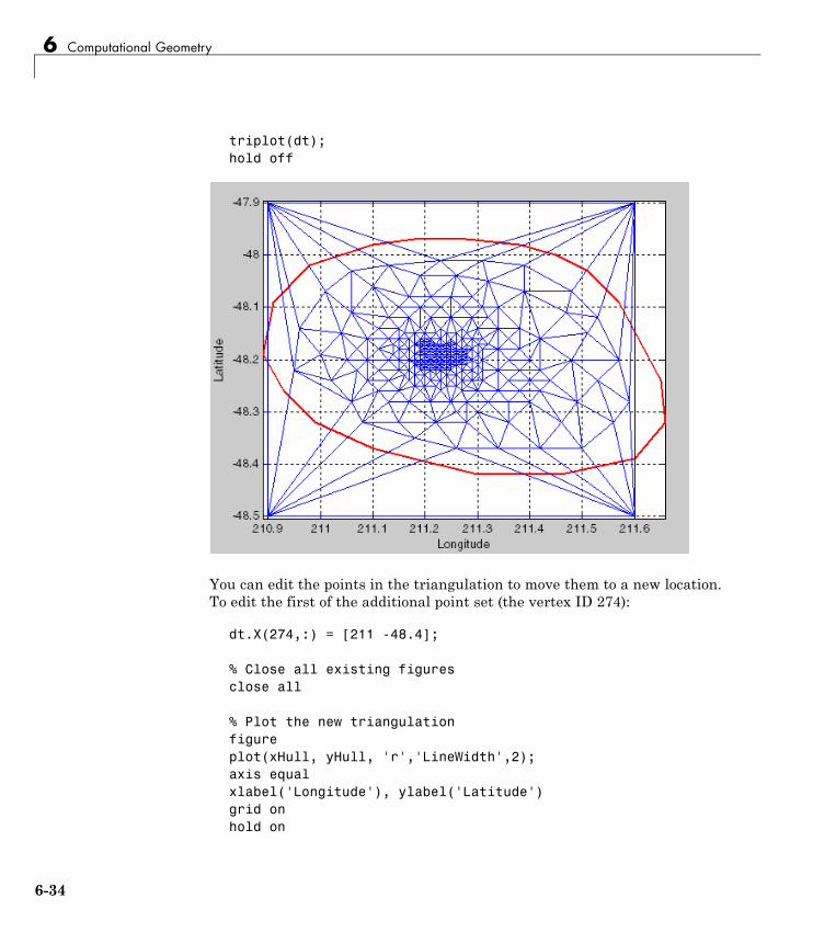
6 Computational Geometry
triplot(dt);hold off
You can edit the points in the triangulation to move them to a new location.To edit the first of the additional point set (the vertex ID 274):
dt.X(274,:) = [211 -48.4];
% Close all existing figuresclose all
% Plot the new triangulationfigureplot(xHull, yHull, 'r','LineWidth',2);axis equalxlabel('Longitude'), ylabel('Latitude')grid onhold on
6-34

Delaunay Triangulation
triplot(dt);hold off
Note TriRep methods are available to DelaunayTri because DelaunayTriis a subclass of TriRep. You can use a TriRep method to query the trianglesattached to the vertex you just moved. Use the vertexAttachmentsmethod tofind the attached triangles. Since the number of triangles attached to a vertexis variable, the method returns the attached triangle indices in a cell array.You need braces to extract the contents.
attTris = vertexAttachments(dt,274);hold ontriplot(dt(attTris{:},:),dt.X(:,1),dt.X(:,2),'g')hold off
6-35
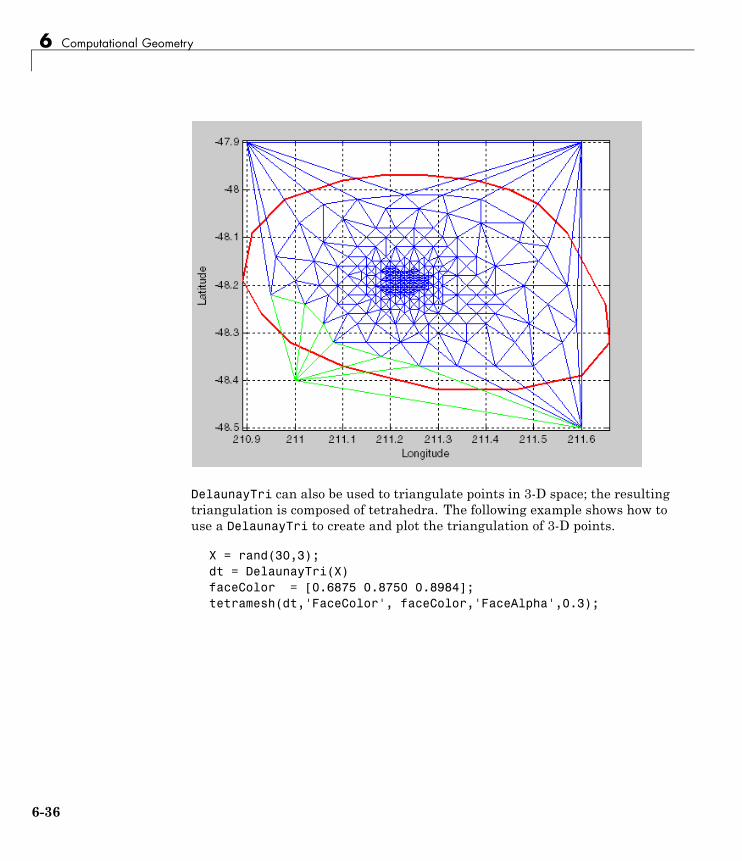
6 Computational Geometry
DelaunayTri can also be used to triangulate points in 3-D space; the resultingtriangulation is composed of tetrahedra. The following example shows how touse a DelaunayTri to create and plot the triangulation of 3-D points.
X = rand(30,3);dt = DelaunayTri(X)faceColor = [0.6875 0.8750 0.8984];tetramesh(dt,'FaceColor', faceColor,'FaceAlpha',0.3);
6-36
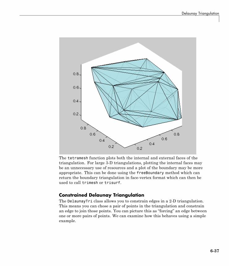
Delaunay Triangulation
The tetramesh function plots both the internal and external faces of thetriangulation. For large 3-D triangulations, plotting the internal faces maybe an unnecessary use of resources and a plot of the boundary may be moreappropriate. This can be done using the freeBoundary method which canreturn the boundary triangulation in face-vertex format which can then beused to call trimesh or trisurf.
Constrained Delaunay TriangulationThe DelaunayTri class allows you to constrain edges in a 2-D triangulation.This means you can chose a pair of points in the triangulation and constrainan edge to join those points. You can picture this as “forcing” an edge betweenone or more pairs of points. We can examine how this behaves using a simpleexample.
6-37
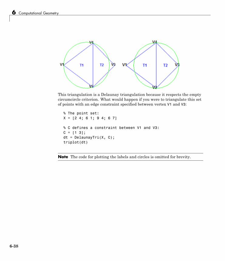
6 Computational Geometry
This triangulation is a Delaunay triangulation because it respects the emptycircumcircle criterion. What would happen if you were to triangulate this setof points with an edge constraint specified between vertex V1 and V3:
% The point set:X = [2 4; 6 1; 9 4; 6 7]
% C defines a constraint between V1 and V3:C = [1 3];dt = DelaunayTri(X, C);triplot(dt)
Note The code for plotting the labels and circles is omitted for brevity.
6-38
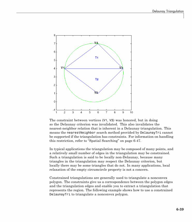
Delaunay Triangulation
The constraint between vertices (V1, V3) was honored, but in doingso the Delaunay criterion was invalidated. This also invalidates thenearest-neighbor relation that is inherent in a Delaunay triangulation. Thismeans the nearestNeighbor search method provided by DelaunayTri cannotbe supported if the triangulation has constraints. For information on handlingthis restriction, refer to “Spatial Searching” on page 6-47.
In typical applications the triangulation may be composed of many points, anda relatively small number of edges in the triangulation may be constrained.Such a triangulation is said to be locally non-Delaunay, because manytriangles in the triangulation may respect the Delaunay criterion, butlocally there may be some triangles that do not. In many applications, localrelaxation of the empty circumcircle property is not a concern.
Constrained triangulations are generally used to triangulate a nonconvexpolygon. The constraints give us a correspondence between the polygon edgesand the triangulation edges and enable you to extract a triangulation thatrepresents the region. The following example shows how to use a constrainedDelaunayTri to triangulate a nonconvex polygon.
6-39
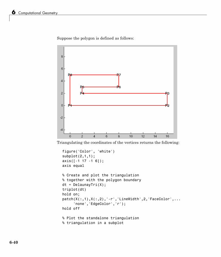
6 Computational Geometry
Suppose the polygon is defined as follows:
Triangulating the coordinates of the vertices returns the following:
figure('Color', 'white')subplot(2,1,1);axis([-1 17 -1 6]);axis equal
% Create and plot the triangulation% together with the polygon boundarydt = DelaunayTri(X);triplot(dt)hold on;patch(X(:,1),X(:,2),'-r','LineWidth',2,'FaceColor',...
'none','EdgeColor','r');hold off
% Plot the standalone triangulation% triangulation in a subplot
6-40
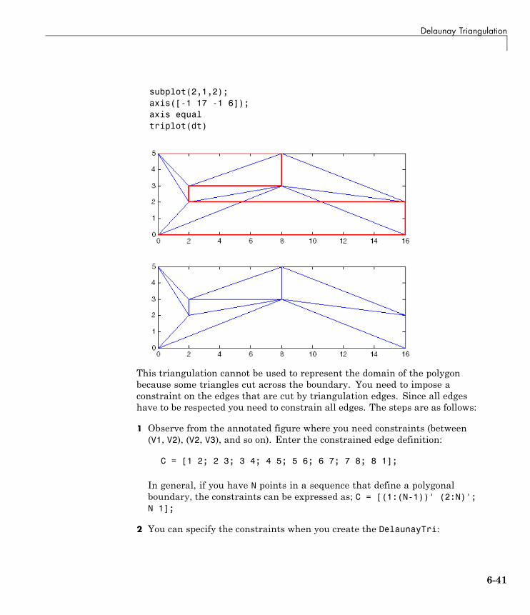
Delaunay Triangulation
subplot(2,1,2);axis([-1 17 -1 6]);axis equaltriplot(dt)
This triangulation cannot be used to represent the domain of the polygonbecause some triangles cut across the boundary. You need to impose aconstraint on the edges that are cut by triangulation edges. Since all edgeshave to be respected you need to constrain all edges. The steps are as follows:
1 Observe from the annotated figure where you need constraints (between(V1, V2), (V2, V3), and so on). Enter the constrained edge definition:
C = [1 2; 2 3; 3 4; 4 5; 5 6; 6 7; 7 8; 8 1];
In general, if you have N points in a sequence that define a polygonalboundary, the constraints can be expressed as; C = [(1:(N-1))' (2:N)';N 1];
2 You can specify the constraints when you create the DelaunayTri:
6-41
6 Computational Geometry
dt = DelaunayTri(X,C)
You can also impose constraints on an existing triangulation by settingthe Constraints property:
dt.Constraints = C;
3 Plot the triangulation and polygon as before:
figure('Color', 'white')subplot(2,1,1);axis([-1 17 -1 6]);axis equal
dt = DelaunayTri(X);triplot(dt)hold on;patch(X(:,1),X(:,2),'-r', 'LineWidth', 2, ...
'FaceColor','none', 'EdgeColor','r');hold off
% Plot the standalone triangulation% triangulation in a subplotsubplot(2,1,2);axis([-1 17 -1 6]);axis equaltriplot(dt)
6-42
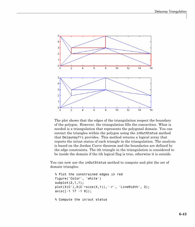
Delaunay Triangulation
The plot shows that the edges of the triangulation respect the boundaryof the polygon. However, the triangulation fills the concavities. What isneeded is a triangulation that represents the polygonal domain. You canextract the triangles within the polygon using the inOutStatus methodthat DelaunayTri provides. This method returns a logical array thatreports the in/out status of each triangle in the triangulation. The analysisis based on the Jordan Curve theorem and the boundaries are defined bythe edge constraints. The ith triangle in the triangulation is considered tobe inside the domain if the ith logical flag is true, otherwise it is outside.
You can now use the inOutStatus method to compute and plot the set ofdomain triangles:
% Plot the constrained edges in redfigure('Color', 'white')subplot(2,1,1);plot(X(C'),X(C'+size(X,1)),'-r', 'LineWidth', 2);axis([-1 17 -1 6]);
% Compute the in/out status
6-43
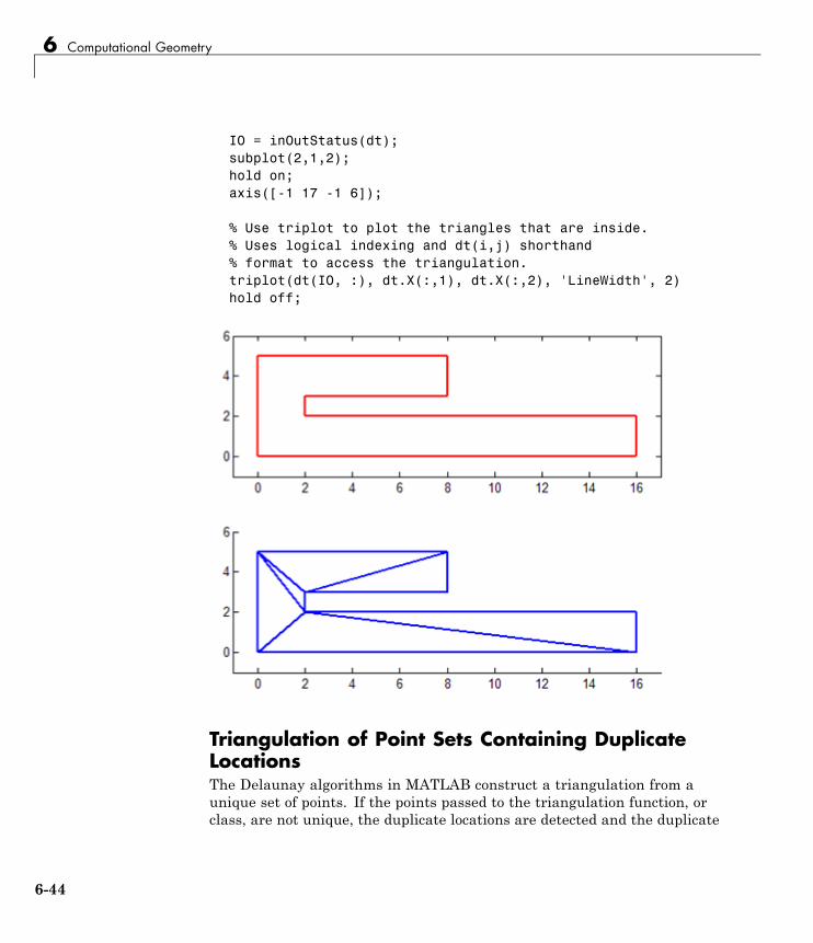
6 Computational Geometry
IO = inOutStatus(dt);subplot(2,1,2);hold on;axis([-1 17 -1 6]);
% Use triplot to plot the triangles that are inside.% Uses logical indexing and dt(i,j) shorthand% format to access the triangulation.triplot(dt(IO, :), dt.X(:,1), dt.X(:,2), 'LineWidth', 2)hold off;
Triangulation of Point Sets Containing DuplicateLocationsThe Delaunay algorithms in MATLAB construct a triangulation from aunique set of points. If the points passed to the triangulation function, orclass, are not unique, the duplicate locations are detected and the duplicate
6-44
Delaunay Triangulation
point is ignored. This produces a triangulation that does not reference somepoints in the original input, namely the duplicate points. When workingwith the delaunay and delaunayn functions the presence of duplicates maybe of little consequence. However, since many of the queries provided bythe DelaunayTri class are index based, it is important to understand thatDelaunayTri triangulates and works with the unique data set. Therefore,indexing based on the unique point set is the convention; this data ismaintained by the X property of DelaunayTri.
The following example illustrates the importance of referencing the uniquedata set stored within the property when working with DelaunayTri:
X = gallery('uniformdata',[25 2],0);X(18,:) = X(8,:)X(16,:) = X(6,:)X(12,:) = X(2,:)
dt = DelaunayTri(X)
When the triangulation is created MATLAB issues a warning. The X propertyshows that the duplicate points have been removed from the data.
dt =
DelaunayTri
Properties:Constraints: []
X: [22x2 double]Triangulation: [31x3 double]
Methods, Superclasses
If for example, the Delaunay triangulation is used to compute the convexhull, the indices of the points on the hull are indices with respect to theunique point set, dt.X. Therefore, to compute and plot the convex hull, thesteps are as follows:
K = dt.convexHull();plot(dt.X(:,1), dt.X(:,2),'.');hold on
6-45
6 Computational Geometry
plot(dt.X(K,1), dt.X(K,2),'-r')
If the original data set containing the duplicates were used in conjunctionwith the indices provided by DelaunayTri then the result would be incorrect.The DelaunayTri works with indices that are based on the unique data setdt.X. For example, the following would produce an incorrect plot, because K isindexed with respect to dt.X and not X:
K = dt.convexHull();plot(X(:,1), X(:,2),'.');hold onplot(X(K,1), X(K,2),'-r')
It’s often more convenient to create a unique data set by removing duplicatesprior to creating the DelaunayTri as it eliminates the potential for confusion.This can be accomplished using the unique function as follows:
X = gallery('uniformdata',[25 2],0);X(18,:) = X(8,:)X(16,:) = X(6,:)X(12,:) = X(2,:)
[~, I, ~] = unique(X,'first','rows');I = sort(I);X = X(I,:);dt = DelaunayTri(X) % The point set is unique
6-46
Spatial Searching
Spatial Searching
In this section...
“Introduction” on page 6-47
“Nearest-Neighbor Search” on page 6-47
“Point Location” on page 6-50
“Searching Non-Delaunay Triangulations” on page 6-53
IntroductionMATLAB provides you with the necessary functions to perform a spatialsearch using a Delaunay triangulation. The Delaunay-based search queriesthat MATLAB supports are:
• Nearest-neighbor search (sometimes called closest-point search orproximity search),
• Point-location search (sometimes called point-in-triangle search orpoint-in-simplex search, where a simplex is a triangle, tetrahedron orhigher dimensional equivalent).
Given a set of points X and a query point q in Euclidean space, thenearest-neighbor search locates a point p in X that is closer to q than to anyother point in X. Given a Delaunay triangulation of X, the point location searchlocates the simplex that contains the query point q.
While MATLAB supports these search schemes in N dimensions, exact spatialsearches usually become prohibitive in 6 dimensions. You should considerapproximate alternatives for large problems in up to 10 dimensions.
Nearest-Neighbor SearchThere are two Delaunay-based approaches to computing nearest neighbors inMATLAB, depending on the dimensionality of the problem:
• For 2-D and 3-D search, use the nearestNeighbor method provided bythe DelaunayTri class.
6-47
6 Computational Geometry
• For 4-D and higher, use the delaunayn function to construct thetriangulation and the complementary dsearchn function to perform thesearch. While these N-D functions support 2-D and 3-D, they are not asefficient as the search methods provided by DelaunayTri.
The following example demonstrates how to perform a nearest-neighborsearch in 2-D with DelaunayTri. Begin by creating a random set of 15 pointsand plotting the points showing ID labels:
X = [3.5 8.2; 6.8 8.3; 1.3 6.5; 3.5 6.3; 5.8 6.2; 8.3 6.5;...1 4; 2.7 4.3; 5 4.5; 7 3.5; 8.7 4.2; 1.5 2.1; 4.1 1.1; ...7 1.5; 8.5 2.75];
Plot the points and add annotations:
plot(X(:,1),X(:,2),'ob')hold onvxlabels = arrayfun(@(n) {sprintf('X%d', n)}, (1:15)');Hpl = text(X(:,1)+0.2, X(:,2)+0.2, vxlabels, 'FontWeight', ...
'bold', 'HorizontalAlignment','center', 'BackgroundColor', ...'none');
hold off
Create a Delaunay triangulation from the points:
dt = DelaunayTri(X);
Create some query points and for each query point find the index of itscorresponding nearest neighbor in X using the nearestNeighbor method:
numq = 10;q = 2+rand(numq,2)*6;xi = nearestNeighbor(dt, q);
Add the query points to the plot and add line segments joining the querypoints to their nearest neighbors:
xnn = X(xi,:);
hold onplot(q(:,1),q(:,2),'or');
6-48
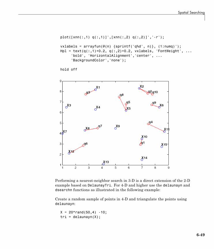
Spatial Searching
plot([xnn(:,1) q(:,1)]',[xnn(:,2) q(:,2)]','-r');
vxlabels = arrayfun(@(n) {sprintf('q%d', n)}, (1:numq)');Hpl = text(q(:,1)+0.2, q(:,2)+0.2, vxlabels, 'FontWeight', ...
'bold', 'HorizontalAlignment','center', ...'BackgroundColor','none');
hold off
Performing a nearest-neighbor search in 3-D is a direct extension of the 2-Dexample based on DelaunayTri. For 4-D and higher use the delaunayn anddsearchn functions as illustrated in the following example:
Create a random sample of points in 4-D and triangulate the points usingdelaunayn:
X = 20*rand(50,4) -10;tri = delaunayn(X);
6-49
6 Computational Geometry
Create some query points and for each query point find the index of itscorresponding nearest neighbor in X using the dsearchn function:
q = rand(5,4);xi = dsearchn(X,tri, q)
The nearestNeighbor method and the dsearchn function allow the Euclideandistance between the query point and its nearest neighbor to be returned asan optional argument. In the 4-D example, you can compute the distances(dnn) as follows:
[xi dnn] = dsearchn(X,tri, q)
Point LocationA point location search is a triangulation-search algorithm that locates thesimplex (triangle, tetrahedron, and so on) enclosing a query point. As in thecase of the nearest-neighbor search, there are two approaches to performinga point-location search in MATLAB, depending on the dimensionality of theproblem:
• For 2-D and 3-D, use the class-based approach with the pointLocationmethod provided by the DelaunayTri class.
• For 4-D and higher, use the delaunayn function to construct thetriangulation and the complementary tsearchn function performs the pointlocation search. Although supporting 2-D and 3-D, these N-D functions arenot as efficient as the search methods provided by DelaunayTri.
The following example demonstrates how to use the DelaunayTri class toperform a point location search in 2-D.
Begin with a set of 2-D points. Create the triangulation and plot it showingthe triangle ID labels at the incenters of the triangles:
X = [3.5 8.2; 6.8 8.3; 1.3 6.5; 3.5 6.3; 5.8 6.2; ...8.3 6.5; 1 4; 2.7 4.3; 5 4.5; 7 3.5; 8.7 4.2; ...1.5 2.1; 4.1 1.1; 7 1.5; 8.5 2.75];
dt = DelaunayTri(X);triplot(dt);
6-50
Spatial Searching
hold onic = incenters(dt);numtri = size(dt,1);trilabels = arrayfun(@(x) {sprintf('T%d', x)}, (1:numtri)');Htl = text(ic(:,1), ic(:,2), trilabels, 'FontWeight', ...
'bold', 'HorizontalAlignment', 'center', 'Color', ...'blue');
hold off
Now create some query points and add them to the plot. Then find the indexof the corresponding enclosing triangles using the pointLocation method:
numq = 10;q = 2+rand(numq,2)*6;hold on;plot(q(:,1),q(:,2),'*r');vxlabels = arrayfun(@(n) {sprintf('q%d', n)}, (1:numq)');Hpl = text(q(:,1)+0.2, q(:,2)+0.2, vxlabels, 'FontWeight', ...
'bold', 'HorizontalAlignment','center', ...'BackgroundColor', 'none');
hold off
ti = pointLocation(dt, q)
6-51
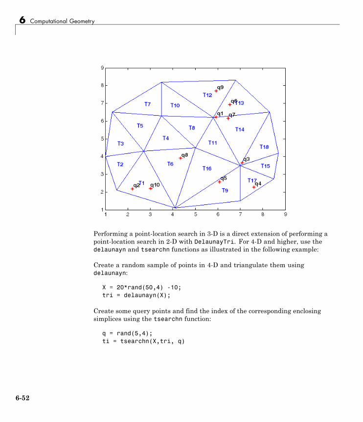
6 Computational Geometry
Performing a point-location search in 3-D is a direct extension of performing apoint-location search in 2-D with DelaunayTri. For 4-D and higher, use thedelaunayn and tsearchn functions as illustrated in the following example:
Create a random sample of points in 4-D and triangulate them usingdelaunayn:
X = 20*rand(50,4) -10;tri = delaunayn(X);
Create some query points and find the index of the corresponding enclosingsimplices using the tsearchn function:
q = rand(5,4);ti = tsearchn(X,tri, q)
6-52
Spatial Searching
The pointLocation method and the tsearchn function allow thecorresponding barycentric coordinates to be returned as an optional argument.In the 4-D example, you can compute the barycentric coordinates as follows:
[ti bc] = tsearchn(X,tri, q)
The barycentric coordinates are useful for performing linear interpolation.These coordinates provide you with weights that you can use to scale thevalues at each vertex of the enclosing simplex. See “Interpolating ScatteredData” on page 7-12 for further details.
Searching Non-Delaunay TriangulationsYou only can use the search functions tsearchn and dsearchn to searchconvex, fully connected Delaunay triangulations that were created inMATLAB. If you create a Delaunay triangulation using delaunayn andsubsequently modify the location of the coordinates, then the Delaunaycriterion could be invalid. Therefore, you should not use the search functionsas they may not converge. The search functions do not check the validity ofthe Delaunay triangulation as this would introduce a significant performancepenalty. Imported triangulations, such as triangulations used for finiteelement analysis, tend to be nonconvex. They could have holes, or they mightnot respect the Delaunay criterion. Hence, you cannot reliably use the searchfunctions tsearchn and dsearchn on triangulations like these.
The class DelaunayTri is more secure in this respect because you only can usethe search methods to search a DelaunayTri. However, you cannot performa nearestNeighbor search on a DelaunayTri that has constrained edgesas it is locally non-Delaunay.
To perform a nearest-neighbor search on a constrained DelaunayTri, do oneof the following:
• Delete the constraints
• Create a new unconstrained DelaunayTri using the same point set, anduse the unconstrained triangulation to perform the search.
Similarly, to perform a nearest-neighbor search on a triangulation that isrepresented in face-vertex format, create a DelaunayTri from the vertexcoordinates and use it to perform the search.
6-53
6 Computational Geometry
MATLAB does not provide dedicated functions for performing a point locationsearch on a 2-D (triangle) or 3-D (tetrahedral) triangulations that are in facevertex format and do not meet the search function requirements. However,for relatively small triangulations a brute-force search might be viable. For a2-D triangulation, you might can recreate the triangulation topology usinga constrained DelaunayTri
You can perform the brute-force search by checking the query point againstevery triangle (or tetrahedron) and selecting the one that contains the point.For example, suppose you have the following triangulation in face-vertexformat and you want to perform a brute-force point location search that findsa triangle enclosing a point.
X = [3.5 8.2; 6.8 8.3; 1.3 6.5; 3.5 6.3; 5.8 6.2; 8.3 6.5; ...1 4; 2.7 4.3; 5 4.5; 7 3.5; 8.7 4.2; 1.5 2.1; 4.1 1.1; ...7 1.5; 8.5 2.75];
tri = delaunay(X);% Remove first triangle to make the triangulation nonconvextri(1,:) = [];
The first thing you can do is create a TriRep to represent this triangulation:
tr = TriRep(tri,X)
The TriRep has many useful query methods, but it does not have apointLocation or a nearestNeighbor method. A TriRep can represent anonconvex triangulation with holes and non-Delaunay triangulations, butthe search algorithms preclude these.
TriRep provides a useful method that you can use to check if a query pointlies within a specified triangle (or tetrahedron). The method is cartToBary.Given a point expressed in Cartesian coordinates and a specified triangle inthe triangulation, this method returns the barycentric coordinates of the pointwith respect to the triangle. If all three barycentric coordinates are positive,the point is within the triangle . Otherwise, the point is outside the triangle.Plot the triangulation to explore this method:
triplot(tr)axis equal
6-54
Spatial Searching
hold onic = incenters(tr);numtri = size(tr,1);trilabels = arrayfun(@(x) {sprintf('T%d', x)}, (1:numtri)');Htl = text(ic(:,1), ic(:,2), trilabels, 'FontWeight', ...
'bold', 'HorizontalAlignment', 'center', 'Color', ...'blue');
hold off
Search for the triangle enclosing (6,3):
numtri = size(tr,1);B = cartToBary(tr, (1:numtri)', repmat([6 3], numtri,1));posB = (B >= 0);enclosingTri = find(posB(:,1) & posB(:,2) & posB(:,3))
You can now use a constrained DelaunayTri to perform the search. Youshould start with the TriRep you created in the brute-force search and use itto find all edges in the triangulation so you can constrain them.:
Cedges = edges(tr);
Now create the constrained DelaunayTri and plot it in a separate figure soyou can compare both triangulations.:
dt = DelaunayTri(X, Cedges)figuretriplot(dt)axis equalhold onic = incenters(dt);numtri = size(dt,1);trilabels = arrayfun(@(x) {sprintf('T%d', x)}, (1:numtri)');Htl = text(ic(:,1), ic(:,2), trilabels, 'FontWeight', ...
'bold', 'HorizontalAlignment', 'center', 'Color', ...'blue');
hold off
Since the triangle numbering is different in each triangle, you need to buildan array of indices to map triangle IDs from the DelaunayTri to the TriRep.
6-55
6 Computational Geometry
To do this mapping you will compute the incenters of the TriRep and find thecorresponding enclosing triangles in the DelaunayTri:
dtTotrIndex = nan(size(dt,1),1);ic = incenters(tr);
dtid = pointLocation(dt,ic)dtTotrIndex(dtid) = 1:size(tr,1);
Now you use the DelaunayTri to perform the point location search. Next, usethe map to find the corresponding triangle in the TriRep:
trid = pointLocation(dt, 6,3);if isfinite(trid)
trid = dtTotrIndex(trid);endtrid
6-56
Voronoi Diagrams
Voronoi DiagramsThe Voronoi diagram of a discrete set of points X decomposes the space aroundeach point X(i) into a region of influence R{i}. This decomposition has theproperty that an arbitrary point P within the region R{i} is closer to point ithan any other point. The region of influence is called a Voronoi region andthe collection of all the Voronoi regions is the Voronoi diagram.
The Voronoi diagram is an N-D geometric construct; however, most practicalapplications are in 2-D and 3-D space. The properties of the Voronoi diagramare best understood using an example. This example uses the 2-D voronoifunction:
figure('Color', 'white')X = [-1.5 3.2; 1.8 3.3; -3.7 1.5; -1.5 1.3; ...
0.8 1.2; 3.3 1.5; -4.0 -1.0;-2.3 -0.7; ...0 -0.5; 2.0 -1.5; 3.7 -0.8; -3.5 -2.9; ...
-0.9 -3.9; 2.0 -3.5; 3.5 -2.25]voronoi(X(:,1),X(:,2))
Assign labels to the points as follows:
nump = size(X,1);plabels = arrayfun(@(n) {sprintf('X%d', n)}, (1:nump)');hold onHpl = text(X(:,1), X(:,2), plabels, 'FontWeight', ...
'bold', 'HorizontalAlignment','center', ...'BackgroundColor', 'none');
Add a query point P at (0, -1.5). Observe that P is closer to X9 than to any otherpoint in X , which is true for any point P within the region that bounds X9:
P = [0 -1];plot(P(1),P(2), '*r');text(P(1), P(2), 'P', 'FontWeight', 'bold', ...
'HorizontalAlignment','center', ...'BackgroundColor', 'none');
hold off
6-57
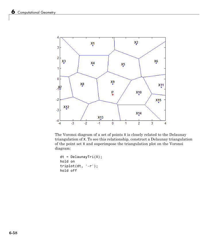
6 Computational Geometry
The Voronoi diagram of a set of points X is closely related to the Delaunaytriangulation of X. To see this relationship, construct a Delaunay triangulationof the point set X and superimpose the triangulation plot on the Voronoidiagram:
dt = DelaunayTri(X);hold ontriplot(dt, '-r');hold off
6-58

Voronoi Diagrams
From the plot you can see that the Voronoi region associated with the point X9is defined by the perpendicular bisectors of the Delaunay edges attached toX9. Also, the vertices of the Voronoi edges are located at the circumcenters ofthe Delaunay triangles. You can illustrate these associations by plotting thecircumcenter of triangle {X9, X4, X8}.
To find the index of this triangle, query the triangulation. The trianglecontains the location (-1, 0):
tidx = dt.pointLocation(-1, 0);
Now, find the circumcenter of this triangle and plot it in green:
cc = dt.circumcenters(tidx);hold onplot(cc(1),cc(2), '*g');hold off
6-59
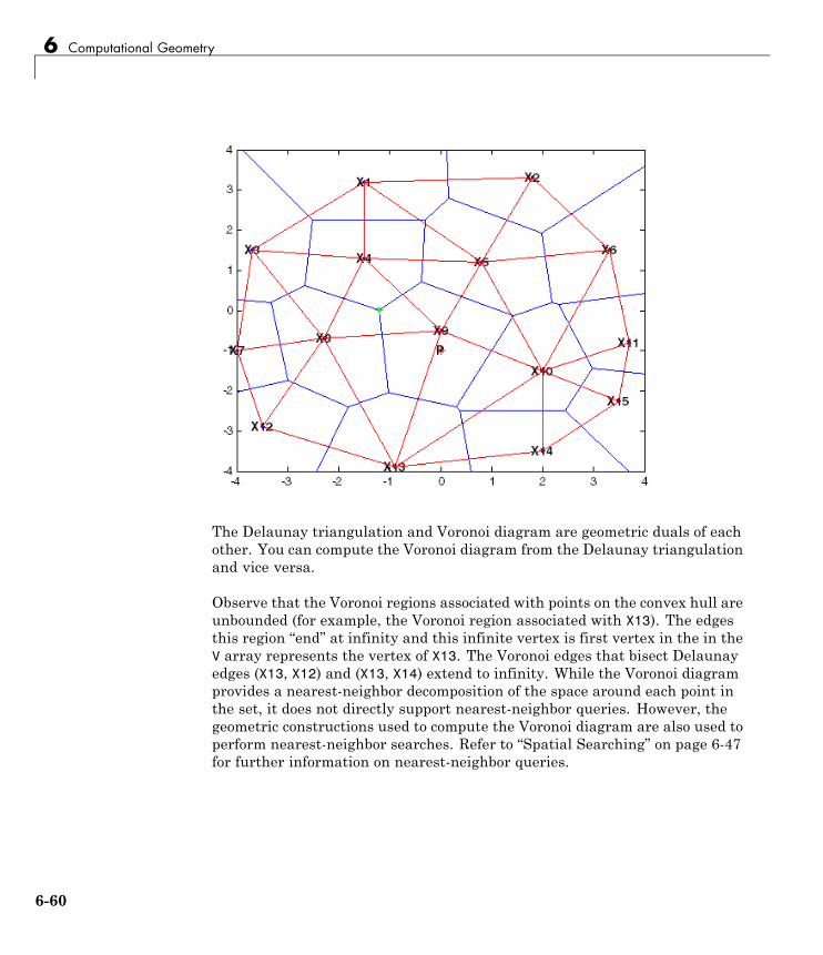
6 Computational Geometry
The Delaunay triangulation and Voronoi diagram are geometric duals of eachother. You can compute the Voronoi diagram from the Delaunay triangulationand vice versa.
Observe that the Voronoi regions associated with points on the convex hull areunbounded (for example, the Voronoi region associated with X13). The edgesthis region “end” at infinity and this infinite vertex is first vertex in the in theV array represents the vertex of X13. The Voronoi edges that bisect Delaunayedges (X13, X12) and (X13, X14) extend to infinity. While the Voronoi diagramprovides a nearest-neighbor decomposition of the space around each point inthe set, it does not directly support nearest-neighbor queries. However, thegeometric constructions used to compute the Voronoi diagram are also used toperform nearest-neighbor searches. Refer to “Spatial Searching” on page 6-47for further information on nearest-neighbor queries.
6-60
Voronoi Diagrams
Computing the Voronoi DiagramMATLAB software provides functions to plot the Voronoi diagram in 2-D andto compute the topology of the Voronoi diagram in N-D. In practice, Voronoicomputation is not practical in dimensions beyond 6-D for moderate to largedata sets, due to the exponential growth in required memory.
The voronoi plot function plots the Voronoi diagram for a set of points in 2-Dspace. In MATLAB there are two ways to compute the topology of the Voronoidiagram of a point set:
• Using the MATLAB function voronoin
• Using the DelaunayTri.voronoiDiagram method provided by theDelaunayTri class.
The voronoin function supports the computation of the Voronoi topology fordiscrete points in N-D (N ≥ 2). The DelaunayTri.voronoiDiagram methodsupports computation of the Voronoi topology for discrete points 2-D or 3-D.
The DelaunayTri.voronoiDiagram method is recommended for 2-D or 3-Dtopology computations as it is more robust and gives better performance forlarge data sets. This method supports incremental insertion and removal ofpoints and complementary queries, such as nearest-neighbor point search.
The voronoin function and the DelaunayTri.voronoiDiagram methodrepresent the topology of the Voronoi diagram using a face-vertex format. See“Triangulation Face-Vertex Format” on page 6-5 for further details on thisdata structure. Given a set of points X, obtain the topology of the Voronoidiagram as follows:
• Using the voronoin function
dt = DelaunayTri(X)[V, R] = dt.voronoiDiagram(X)
• Using the DelaunayTri.voronoiDiagram method
dt = DelaunayTri(X)[V, R] = dt.voronoiDiagram(X)
6-61
6 Computational Geometry
V is a matrix representing the coordinates of the Voronoi vertices (the verticesare the end points of the Voronoi edges). R is a vector cell array lengthsize(X,1), representing the Voronoi region associated with each point.Hence, the Voronoi region associated with the ith point X(i) is R{i}.
Reusing the previous data helps to clarify the V, R datastructure.
X = [-1.5 3.2; 1.8 3.3; -3.7 1.5; -1.5 1.3; 0.8 1.2; ...3.3 1.5; -4.0 -1.0; -2.3 -0.7; 0 -0.5; 2.0 -1.5; ...3.7 -0.8; -3.5 -2.9; -0.9 -3.9; 2.0 -3.5; 3.5 -2.25]
[VX, VY] = voronoi(X(:,1),X(:,2));h = plot(VX,VY,'-b',X(:,1),X(:,2),'.r');set(h(1:end-1),'xliminclude','off','yliminclude','off')
Assign labels to the points X:
nump = size(X,1);plabels = arrayfun(@(n) {sprintf('X%d', n)}, (1:nump)');hold onHpl = text(X(:,1), X(:,2)+0.2, plabels, 'color', 'r', ...
'FontWeight', 'bold', 'HorizontalAlignment',...'center', 'BackgroundColor', 'none');
Compute the Voronoi diagram:
dt = DelaunayTri(X);[V R] = dt.voronoiDiagram();
Assign labels to the Voronoi vertices V. By convention the first vertex is atinfinity:
numv = size(V,1);vlabels = arrayfun(@(n) {sprintf('V%d', n)}, (2:numv)');hold onHpl = text(V(2:end,1), V(2:end,2)+.2, vlabels, ...
'FontWeight', 'bold', 'HorizontalAlignment',...'center', 'BackgroundColor', 'none');
6-62
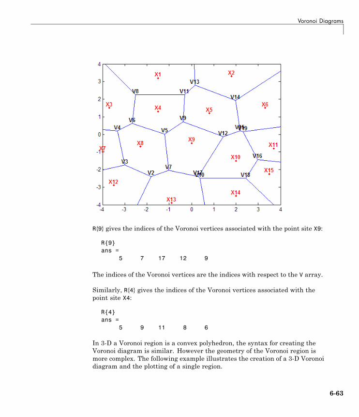
Voronoi Diagrams
R{9} gives the indices of the Voronoi vertices associated with the point site X9:
R{9}ans =
5 7 17 12 9
The indices of the Voronoi vertices are the indices with respect to the V array.
Similarly, R{4} gives the indices of the Voronoi vertices associated with thepoint site X4:
R{4}ans =
5 9 11 8 6
In 3-D a Voronoi region is a convex polyhedron, the syntax for creating theVoronoi diagram is similar. However the geometry of the Voronoi region ismore complex. The following example illustrates the creation of a 3-D Voronoidiagram and the plotting of a single region.
6-63
6 Computational Geometry
Create a sample of 25 points in 3-D space and compute the topology of theVoronoi diagram for this point set:
X = -3 + 6.*gallery('uniformdata',[25 3],0);dt = DelaunayTri(X)
Compute the topology of the Voronoi diagram:
[V R] = dt.voronoiDiagram();
Find the point closest to the origin and plot the Voronoi region associatedwith this point:
tid = dt.nearestNeighbor(0,0,0)XR10 = V(R{tid},:)
K = convhull(XR10);defaultFaceColor = [0.6875 0.8750 0.8984]trisurf(K, XR10(:,1) ,XR10(:,2) ,XR10(:,3) , ...
'FaceColor', defaultFaceColor, 'FaceAlpha',0.8);
6-64
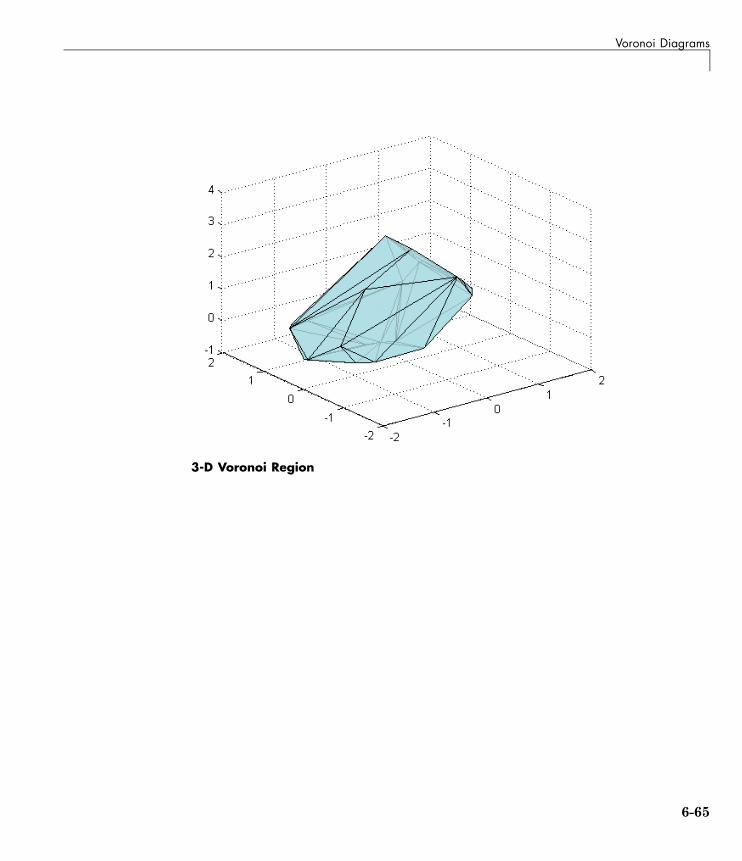
Voronoi Diagrams
3-D Voronoi Region
6-65
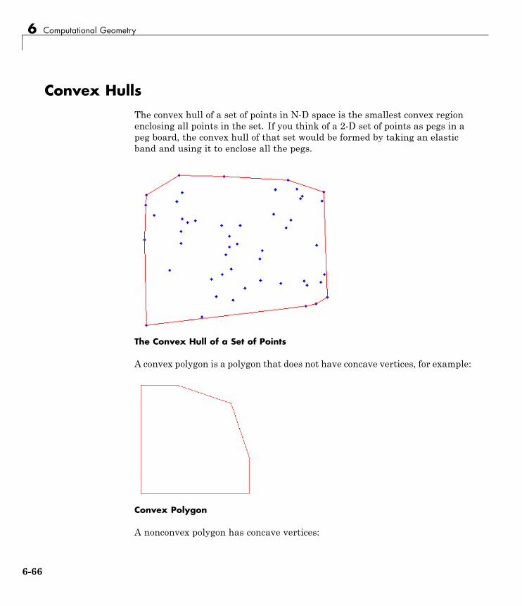
6 Computational Geometry
Convex HullsThe convex hull of a set of points in N-D space is the smallest convex regionenclosing all points in the set. If you think of a 2-D set of points as pegs in apeg board, the convex hull of that set would be formed by taking an elasticband and using it to enclose all the pegs.
The Convex Hull of a Set of Points
A convex polygon is a polygon that does not have concave vertices, for example:
Convex Polygon
A nonconvex polygon has concave vertices:
6-66
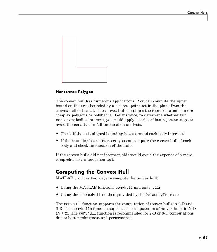
Convex Hulls
Nonconvex Polygon
The convex hull has numerous applications. You can compute the upperbound on the area bounded by a discrete point set in the plane from theconvex hull of the set. The convex hull simplifies the representation of morecomplex polygons or polyhedra. For instance, to determine whether twononconvex bodies intersect, you could apply a series of fast rejection steps toavoid the penalty of a full intersection analysis:
• Check if the axis-aligned bounding boxes around each body intersect.
• If the bounding boxes intersect, you can compute the convex hull of eachbody and check intersection of the hulls.
If the convex hulls did not intersect, this would avoid the expense of a morecomprehensive intersection test.
Computing the Convex HullMATLAB provides two ways to compute the convex hull:
• Using the MATLAB functions convhull and convhulln
• Using the convexHull method provided by the DelaunayTri class
The convhull function supports the computation of convex hulls in 2-D and3-D. The convhulln function supports the computation of convex hulls in N-D(N ≥ 2). The convhull function is recommended for 2-D or 3-D computationsdue to better robustness and performance.
6-67
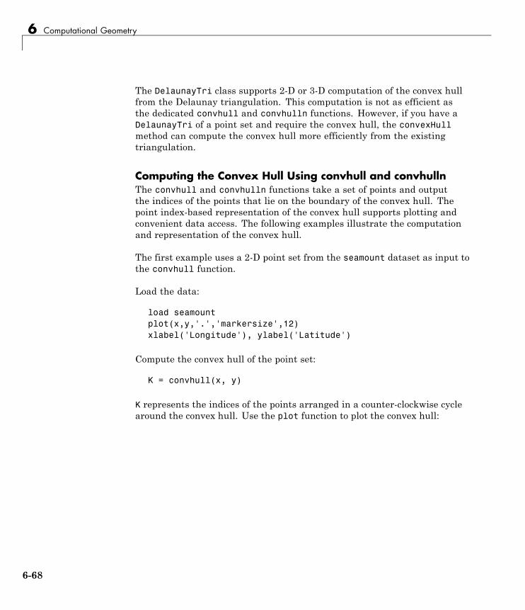
6 Computational Geometry
The DelaunayTri class supports 2-D or 3-D computation of the convex hullfrom the Delaunay triangulation. This computation is not as efficient asthe dedicated convhull and convhulln functions. However, if you have aDelaunayTri of a point set and require the convex hull, the convexHullmethod can compute the convex hull more efficiently from the existingtriangulation.
Computing the Convex Hull Using convhull and convhullnThe convhull and convhulln functions take a set of points and outputthe indices of the points that lie on the boundary of the convex hull. Thepoint index-based representation of the convex hull supports plotting andconvenient data access. The following examples illustrate the computationand representation of the convex hull.
The first example uses a 2-D point set from the seamount dataset as input tothe convhull function.
Load the data:
load seamountplot(x,y,'.','markersize',12)xlabel('Longitude'), ylabel('Latitude')
Compute the convex hull of the point set:
K = convhull(x, y)
K represents the indices of the points arranged in a counter-clockwise cyclearound the convex hull. Use the plot function to plot the convex hull:
6-68
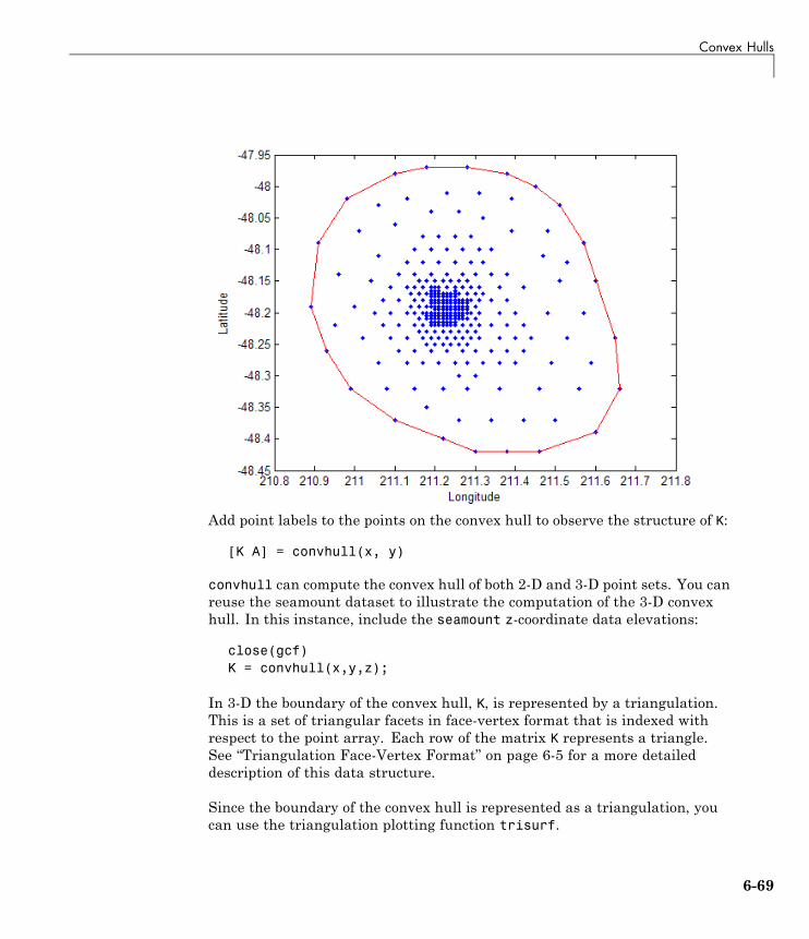
Convex Hulls
Add point labels to the points on the convex hull to observe the structure of K:
[K A] = convhull(x, y)
convhull can compute the convex hull of both 2-D and 3-D point sets. You canreuse the seamount dataset to illustrate the computation of the 3-D convexhull. In this instance, include the seamount z-coordinate data elevations:
close(gcf)K = convhull(x,y,z);
In 3-D the boundary of the convex hull, K, is represented by a triangulation.This is a set of triangular facets in face-vertex format that is indexed withrespect to the point array. Each row of the matrix K represents a triangle.See “Triangulation Face-Vertex Format” on page 6-5 for a more detaileddescription of this data structure.
Since the boundary of the convex hull is represented as a triangulation, youcan use the triangulation plotting function trisurf.
6-69
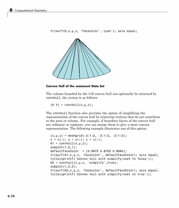
6 Computational Geometry
trisurf(K,x,y,z, 'Facecolor','cyan'); axis equal;
Convex Hull of the seamount Data Set
The volume bounded by the 3-D convex hull can optionally be returned byconvhull, the syntax is as follows:
[K V] = convhull(x,y,z);
The convhull function also provides the option of simplifying therepresentation of the convex hull by removing vertices that do not contributeto the area or volume. For example, if boundary facets of the convex hullare collinear or coplanar, you can merge them to give a more conciserepresentation. The following example illustrates use of this option:
[x,y,z] = meshgrid(-2:1:2, -2:1:2, -2:1:2);x = x(:); y = y(:); z = z(:);K1 = convhull(x,y,z);subplot(1,2,1);defaultFaceColor = [0.6875 0.8750 0.8984];trisurf(K1,x,y,z, 'Facecolor', defaultFaceColor); axis equal;title(sprintf('Convex hull with simplify\nset to false'));K2 = convhull(x,y,z, 'simplify',true);subplot(1,2,2);trisurf(K2,x,y,z, 'Facecolor', defaultFaceColor); axis equal;title(sprintf('Convex hull with simplify\nset to true'));
6-70
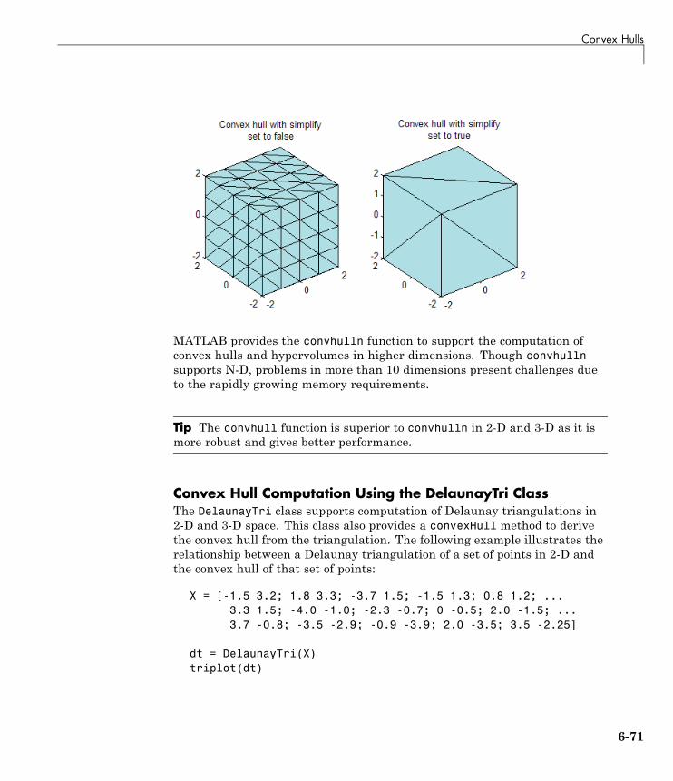
Convex Hulls
MATLAB provides the convhulln function to support the computation ofconvex hulls and hypervolumes in higher dimensions. Though convhullnsupports N-D, problems in more than 10 dimensions present challenges dueto the rapidly growing memory requirements.
Tip The convhull function is superior to convhulln in 2-D and 3-D as it ismore robust and gives better performance.
Convex Hull Computation Using the DelaunayTri ClassThe DelaunayTri class supports computation of Delaunay triangulations in2-D and 3-D space. This class also provides a convexHull method to derivethe convex hull from the triangulation. The following example illustrates therelationship between a Delaunay triangulation of a set of points in 2-D andthe convex hull of that set of points:
X = [-1.5 3.2; 1.8 3.3; -3.7 1.5; -1.5 1.3; 0.8 1.2; ...3.3 1.5; -4.0 -1.0; -2.3 -0.7; 0 -0.5; 2.0 -1.5; ...3.7 -0.8; -3.5 -2.9; -0.9 -3.9; 2.0 -3.5; 3.5 -2.25]
dt = DelaunayTri(X)triplot(dt)
6-71
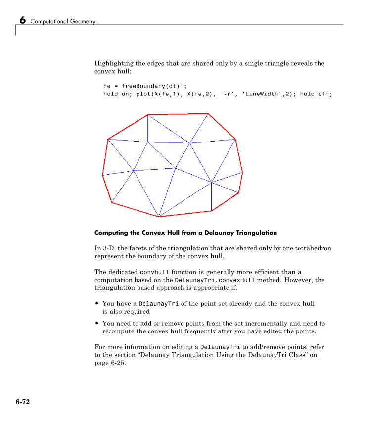
6 Computational Geometry
Highlighting the edges that are shared only by a single triangle reveals theconvex hull:
fe = freeBoundary(dt)';hold on; plot(X(fe,1), X(fe,2), '-r', 'LineWidth',2); hold off;
Computing the Convex Hull from a Delaunay Triangulation
In 3-D, the facets of the triangulation that are shared only by one tetrahedronrepresent the boundary of the convex hull.
The dedicated convhull function is generally more efficient than acomputation based on the DelaunayTri.convexHull method. However, thetriangulation based approach is appropriate if:
• You have a DelaunayTri of the point set already and the convex hullis also required
• You need to add or remove points from the set incrementally and need torecompute the convex hull frequently after you have edited the points.
For more information on editing a DelaunayTri to add/remove points, referto the section “Delaunay Triangulation Using the DelaunayTri Class” onpage 6-25.
6-72
7
Interpolation
• “Interpolating Structured Data” on page 7-3
• “Interpolating Scattered Data” on page 7-12
Interpolation is a method for estimating the value at a query location that lieswithin the domain of a set of sample data points. A sample data set definedby locations X and corresponding values V can be interpolated to produce afunction of the form V = F(X). This function can then be used to evaluate aquery point Xq, to give Vq = F(Xq). This is a single-valued function; for anyquery Xq within the domain of X it will produce a unique value Vq. The sampledata is assumed to respect this property in order to produce a satisfactoryinterpolation. One other interesting characteristic is that the interpolatingfunction passes through the data points. This is an important distinctionbetween interpolation and curve/surface fitting. In fitting, the function doesnot necessarily pass through the sample data points.
The computation of the value Vq is generally based on the data points inthe neighborhood of the query point Xq. There are numerous approaches toperforming interpolation. In MATLAB interpolation is classified into twocategories depending on the structure of the sample data. The sample datamay be ordered in a Cartesian axis-aligned grid or they may be scattered.In the case of a gridded distribution of sample points, you can leverage theorganized structure of the data to efficiently find the sample points in theneighborhood of the query. Interpolation of scattered data on the other handrequires a triangulation of the data points, and this introduces an additionallevel of computation.
The two approaches to interpolation are covered in the following sections:
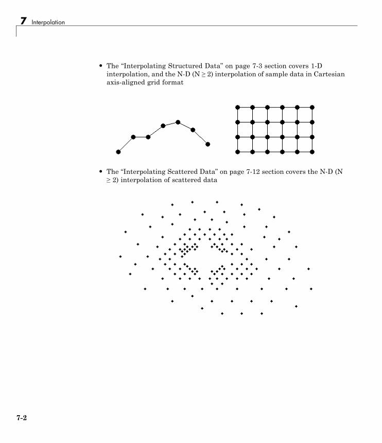
7 Interpolation
• The “Interpolating Structured Data” on page 7-3 section covers 1-Dinterpolation, and the N-D (N ≥ 2) interpolation of sample data in Cartesianaxis-aligned grid format
• The “Interpolating Scattered Data” on page 7-12 section covers the N-D (N≥ 2) interpolation of scattered data
7-2
Interpolating Structured Data
Interpolating Structured Data
In this section...
“One-Dimensional Data” on page 7-3
“Two-Dimensional Data” on page 7-5
“Multidimensional Data” on page 7-8
One-Dimensional Data
• “Polynomial Interpolation” on page 7-3
• “FFT-Based Interpolation” on page 7-4
Polynomial InterpolationThe function interp1 performs one-dimensional interpolation. This functionuses polynomial techniques, fitting the supplied data with polynomialfunctions between data points and evaluating the appropriate function at thedesired interpolation points. Its most general form is
yi = interp1(x,y,xi,method)
y is a vector containing the values of a function, and x is a vector of the samelength containing the points for which the values in y are given. xi is a vectorcontaining the points at which to interpolate. method is an optional stringspecifying an interpolation method:
• Nearest neighbor interpolation (method = 'nearest'). This method setsthe value of an interpolated point to the value of the nearest existingdata point.
• Linear interpolation (method = 'linear'). This method fits a differentlinear function between each pair of existing data points, and returns thevalue of the relevant function at the points specified by xi. This is thedefault method for the interp1 function.
• Cubic spline interpolation (method = 'spline'). This method fits adifferent cubic function between each pair of existing data points, and usesthe spline function to perform cubic spline interpolation at the data points.
7-3
7 Interpolation
• Cubic interpolation (method = 'pchip' or 'cubic'). These methodsare identical. They use the pchip function to perform piecewise cubicHermite interpolation within the vectors x and y. These methods preservemonotonicity and the shape of the data.
If any element of xi is outside the interval spanned by x, thespecified interpolation method is used for extrapolation. Alternatively,yi = interp1(x,Y,xi,method,extrapval) replaces extrapolated valueswith extrapval. NaN is often used for extrapval.
All methods work with nonuniformly spaced data.
Speed, Memory, and Smoothness Considerations. When choosing aninterpolation method, keep in mind that some require more memory or longercomputation time than others. However, you may need to trade off theseresources to achieve the desired smoothness in the result:
• Nearest neighbor interpolation is the fastest method. However, it providesthe worst results in terms of smoothness.
• Linear interpolation uses more memory than the nearest neighbor method,and requires slightly more execution time. Unlike nearest neighborinterpolation its results are continuous, but the slope changes at the vertexpoints.
• Cubic spline interpolation has the longest relative execution time, althoughit requires less memory than cubic interpolation. It produces the smoothestresults of all the interpolation methods. You may obtain unexpectedresults, however, if your input data is nonuniform and some points aremuch closer together than others.
• Cubic interpolation requires more memory and execution time than eitherthe nearest neighbor or linear methods. However, both the interpolateddata and its derivative are continuous.
FFT-Based InterpolationThe function interpft performs one-dimensional interpolation using anFFT-based method. This method calculates the Fourier transform of a vectorthat contains the values of a periodic function. It then calculates the inverseFourier transform using more points. Its form is
7-4
Interpolating Structured Data
y = interpft(x,n)
x is a vector containing the values of a periodic function, sampled at equallyspaced points. n is the number of equally spaced points to return.
Two-Dimensional Data
• “Two-Dimensional Methods” on page 7-5
• “A Comparison of Methods” on page 7-6
Two-Dimensional MethodsThe function interp2 performs two-dimensional interpolation, an importantoperation for image processing and data visualization. Its most general form is
ZI = interp2(X,Y,Z,XI,YI,method)
Z is a rectangular array containing the values of a two-dimensional function,and X and Y are arrays of the same size containing the points for which thevalues in Z are given. XI and YI are matrices containing the points at which tointerpolate the data. method is an optional string specifying an interpolationmethod.
There are three different interpolation methods for two-dimensional data:
• Nearest neighbor interpolation (method = 'nearest'). This method fitsa piecewise constant surface through the data values. The value of aninterpolated point is the value of the nearest point.
• Bilinear interpolation (method = 'linear'). This method fits a bilinearsurface through existing data points. The value of an interpolated pointis a combination of the values of the four closest points. This method ispiecewise bilinear, and is faster and less memory-intensive than bicubicinterpolation.
• Bicubic interpolation (method = 'cubic'). This method fits a bicubicsurface through existing data points. The value of an interpolated pointis a combination of the values of the sixteen closest points. This methodis piecewise bicubic, and produces a much smoother surface than bilinearinterpolation. This can be a key advantage for applications like image
7-5
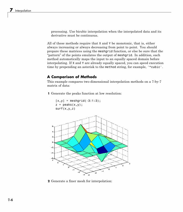
7 Interpolation
processing. Use bicubic interpolation when the interpolated data and itsderivative must be continuous.
All of these methods require that X and Y be monotonic, that is, eitheralways increasing or always decreasing from point to point. You shouldprepare these matrices using the meshgrid function, or else be sure that the“pattern” of the points emulates the output of meshgrid. In addition, eachmethod automatically maps the input to an equally spaced domain beforeinterpolating. If X and Y are already equally spaced, you can speed executiontime by prepending an asterisk to the method string, for example, '*cubic'.
A Comparison of MethodsThis example compares two-dimensional interpolation methods on a 7-by-7matrix of data:
1 Generate the peaks function at low resolution:
[x,y] = meshgrid(-3:1:3);z = peaks(x,y);surf(x,y,z)
2 Generate a finer mesh for interpolation:
7-6
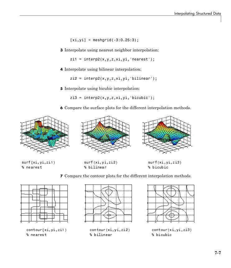
Interpolating Structured Data
[xi,yi] = meshgrid(-3:0.25:3);
3 Interpolate using nearest neighbor interpolation:
zi1 = interp2(x,y,z,xi,yi,'nearest');
4 Interpolate using bilinear interpolation:
zi2 = interp2(x,y,z,xi,yi,'bilinear');
5 Interpolate using bicubic interpolation:
zi3 = interp2(x,y,z,xi,yi,'bicubic');
6 Compare the surface plots for the different interpolation methods.
7 Compare the contour plots for the different interpolation methods.
7-7
7 Interpolation
Notice that the bicubic method, in particular, produces smoother contours.This is not always the primary concern, however. For some applications, suchas medical image processing, a method like nearest neighbor may be preferredbecause it doesn’t generate any “new” data values.
Multidimensional Data
• “Function Summary” on page 7-8
• “Interpolation of Three-Dimensional Data” on page 7-8
• “Interpolation of Higher Dimensional Data” on page 7-9
• “Multidimensional Data Gridding” on page 7-10
Function SummaryThe following table lists functions that operate specifically onmultidimensional data.
Interpolation Functions for Multidimensional Data
Function Description
interp3 Three-dimensional data interpolation
interpn Multidimensional data interpolation
ndgrid Multidimensional data gridding (elmat directory)
Interpolation of Three-Dimensional DataThe function interp3 performs three-dimensional interpolation, findinginterpolated values between points of a three-dimensional set of samples V.You must specify a set of known data points:
• X, Y, and Z matrices specify the points for which values of V are given.
• A matrix V contains values corresponding to the points in X, Y, and Z.
The most general form for interp3 is
VI = interp3(X,Y,Z,V,XI,YI,ZI,method)
7-8
Interpolating Structured Data
XI, YI, and ZI are the points at which interp3 interpolates values of V. Forout-of-range values, interp3 returns NaN.
There are three different interpolation methods for three-dimensional data:
• Nearest neighbor interpolation (method = 'nearest'). This methodchooses the value of the nearest point.
• Trilinear interpolation (method = 'linear'). This method uses piecewiselinear interpolation based on the values of the nearest eight points.
• Tricubic interpolation (method = 'cubic'). This method uses piecewisecubic interpolation based on the values of the nearest sixty-four points.
All of these methods require that X, Y, and Z be monotonic, that is, eitheralways increasing or always decreasing in a particular direction. In addition,you should prepare these matrices using the meshgrid function, or else besure that the “pattern” of the points emulates the output of meshgrid.
Each method automatically maps the input to an equally spaced domainbefore interpolating. If x is already equally spaced, you can speed executiontime by prepending an asterisk to the method string, for example, '*cubic'.
Interpolation of Higher Dimensional DataThe function interpn performs multidimensional interpolation, findinginterpolated values between points of a multidimensional set of samples V.The most general form for interpn is
VI = interpn(X1,X2,X3...,V,Y1,Y2,Y3,...,method)
1, 2, 3, ... are matrices that specify the points for which values of V aregiven. V is a matrix that contains the values corresponding to these points.1, 2, 3, ... are the points for which interpn returns interpolated values ofV. For out-of-range values, interpn returns NaN.
Y1, Y2, Y3, ... must be either arrays of the same size, or vectors. If theyare vectors of different sizes, interpn passes them to ndgrid and then usesthe resulting arrays.
7-9
7 Interpolation
There are three different interpolation methods for multidimensional data:
• Nearest neighbor interpolation (method = 'nearest'). This methodchooses the value of the nearest point.
• Linear interpolation (method = 'linear'). This method uses piecewiselinear interpolation based on the values of the nearest two points in eachdimension.
• Cubic interpolation (method = 'cubic'). This method uses piecewisecubic interpolation based on the values of the nearest four points in eachdimension.
All of these methods require that X1, X2,X3 be monotonic. In addition, youshould prepare these matrices using the ndgrid function, or else be sure thatthe “pattern” of the points emulates the output of ndgrid.
Each method automatically maps the input to an equally spaced domainbefore interpolating. If X is already equally spaced, you can speed executiontime by prepending an asterisk to the method string; for example, '*cubic'.
Multidimensional Data GriddingThe ndgrid function generates arrays of data for multidimensional functionevaluation and interpolation. ndgrid transforms the domain specified by aseries of input vectors into a series of output arrays. The ith dimension ofthese output arrays are copies of the elements of input vector xi.
The syntax for ndgrid is
[X1,X2,X3,...] = ndgrid(x1,x2,x3,...)
For example, assume that you want to evaluate a function of three variablesover a given range. Consider the function
for , , and . To evaluate and plot thisfunction,
x1 = -2:0.2:2;
7-10
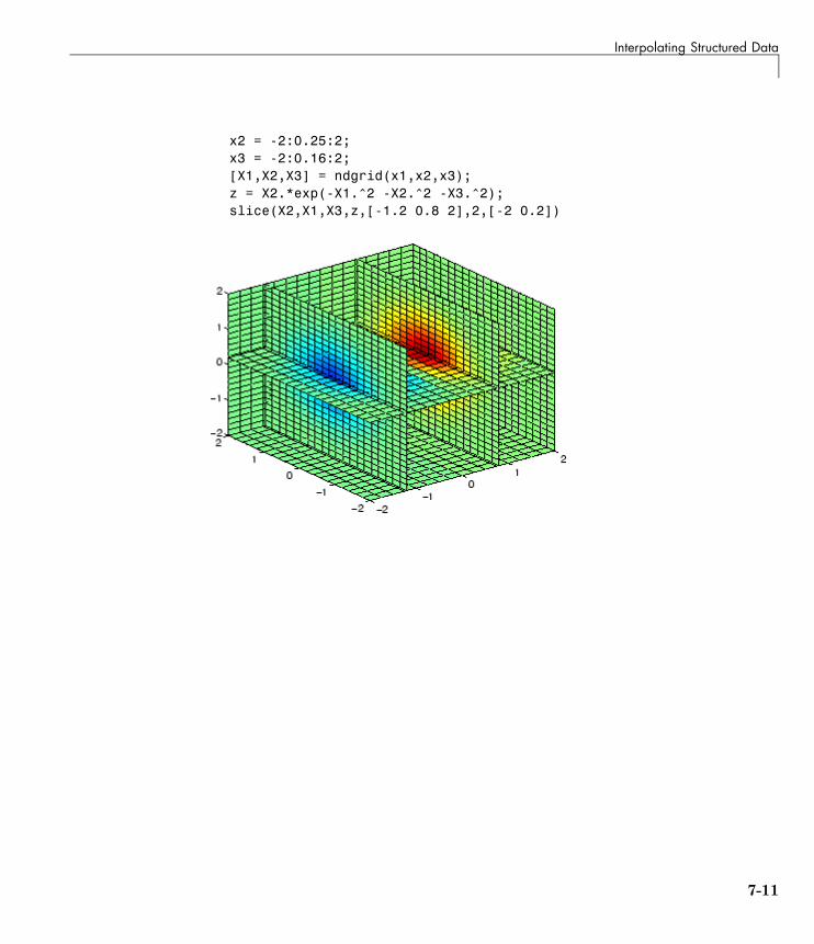
Interpolating Structured Data
x2 = -2:0.25:2;x3 = -2:0.16:2;[X1,X2,X3] = ndgrid(x1,x2,x3);z = X2.*exp(-X1.^2 -X2.^2 -X3.^2);slice(X2,X1,X3,z,[-1.2 0.8 2],2,[-2 0.2])
7-11
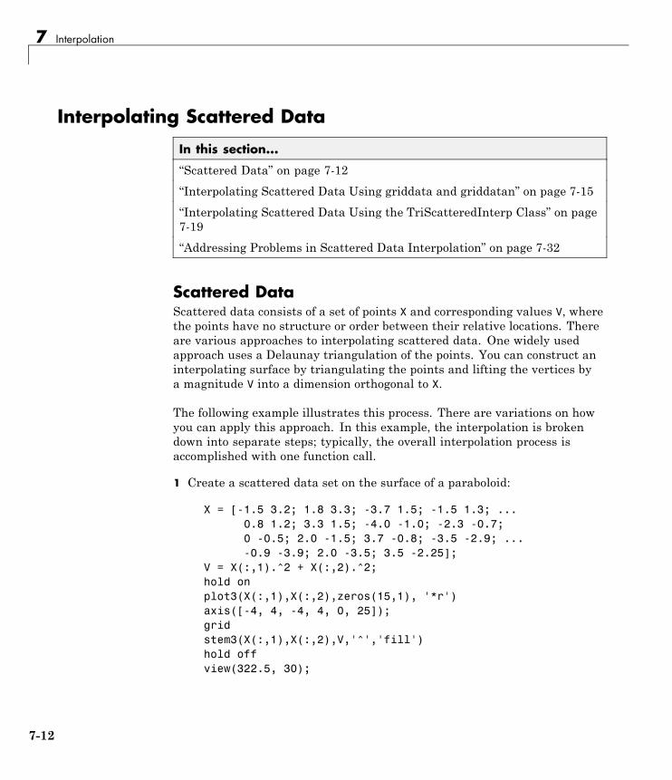
7 Interpolation
Interpolating Scattered Data
In this section...
“Scattered Data” on page 7-12
“Interpolating Scattered Data Using griddata and griddatan” on page 7-15
“Interpolating Scattered Data Using the TriScatteredInterp Class” on page7-19
“Addressing Problems in Scattered Data Interpolation” on page 7-32
Scattered DataScattered data consists of a set of points X and corresponding values V, wherethe points have no structure or order between their relative locations. Thereare various approaches to interpolating scattered data. One widely usedapproach uses a Delaunay triangulation of the points. You can construct aninterpolating surface by triangulating the points and lifting the vertices bya magnitude V into a dimension orthogonal to X.
The following example illustrates this process. There are variations on howyou can apply this approach. In this example, the interpolation is brokendown into separate steps; typically, the overall interpolation process isaccomplished with one function call.
1 Create a scattered data set on the surface of a paraboloid:
X = [-1.5 3.2; 1.8 3.3; -3.7 1.5; -1.5 1.3; ...0.8 1.2; 3.3 1.5; -4.0 -1.0; -2.3 -0.7;0 -0.5; 2.0 -1.5; 3.7 -0.8; -3.5 -2.9; ...-0.9 -3.9; 2.0 -3.5; 3.5 -2.25];
V = X(:,1).^2 + X(:,2).^2;hold onplot3(X(:,1),X(:,2),zeros(15,1), '*r')axis([-4, 4, -4, 4, 0, 25]);gridstem3(X(:,1),X(:,2),V,'^','fill')hold offview(322.5, 30);
7-12

Interpolating Scattered Data
2 Create a Delaunay triangulation and lift the vertices:
figure('Color', 'white')t = delaunay(X(:,1),X(:,2));
hold on
trimesh(t,X(:,1),X(:,2), zeros(15,1), ...'EdgeColor','r', 'FaceColor','none')
defaultFaceColor = [0.6875 0.8750 0.8984];trisurf(t,X(:,1),X(:,2), V, 'FaceColor', ...
defaultFaceColor, 'FaceAlpha',0.9);plot3(X(:,1),X(:,2),zeros(15,1), '*r')axis([-4, 4, -4, 4, 0, 25]);gridplot3(-2.6,-2.6,0,'*b','LineWidth', 1.6)plot3([-2.6 -2.6]',[-2.6 -2.6]',[0 13.52]','-b','LineWidth',1.6)hold off
7-13
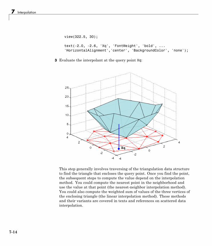
7 Interpolation
view(322.5, 30);
text(-2.0, -2.6, 'Xq', 'FontWeight', 'bold', ...'HorizontalAlignment','center', 'BackgroundColor', 'none');
3 Evaluate the interpolant at the query point Xq:
This step generally involves traversing of the triangulation data structureto find the triangle that encloses the query point. Once you find the point,the subsequent steps to compute the value depend on the interpolationmethod. You could compute the nearest point in the neighborhood anduse the value at that point (the nearest-neighbor interpolation method).You could also compute the weighted sum of values of the three vertices ofthe enclosing triangle (the linear interpolation method). These methodsand their variants are covered in texts and references on scattered datainterpolation.
7-14
Interpolating Scattered Data
Though the illustration highlights 2-D interpolation, you can apply thistechnique to higher dimensions. In more general terms, given a set of points Xand corresponding values V, you can construct an interpolant of the form V =F(X). You can evaluate the interpolant at a query point Xq, to give Vq = F(Xq).This is a single-valued function; for any query point Xq within the convex hullof X it will produce a unique value Vq. The sample data is assumed to respectthis property in order to produce a satisfactory interpolation.
MATLAB provides two ways to perform triangulation-based scattered datainterpolation:
• The functions griddata and griddatan
• The TriScatteredInterp class
The griddata function supports N-D scattered data interpolation. Thegriddatan function supports scattered data interpolation in N-D; however,it is not practical in dimensions higher than 6-D for moderate to large pointsets, due to the exponential growth in memory required by the underlyingtriangulation.
The TriScatteredInterp class supports scattered data interpolation in 2-Dand 3-D space. Use of this class is encouraged as it is more efficient andreadily adapts to a wider range of interpolation problems. In addition, thecalling syntax is more intuitive.
Interpolating Scattered Data Using griddata andgriddatanThe griddata and griddatan functions take a set of sample points X,corresponding values V, and query points Xq and return the interpolatedvalues Vq. The calling syntax is similar for each function; the distinction is the2-D griddata function lets you define the points in terms of X, Y coordinates.These two functions interpolate scattered data at predefined grid-pointlocations; the intent is to produce gridded data, hence the name. Interpolationis more general in practice. You might want to query at arbitrary locationswithin the convex hull of the points.
The following example demonstrates how the griddata function interpolatesscattered data at a set of grid points and uses this gridded data to create a
7-15
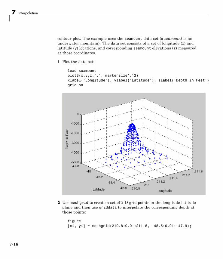
7 Interpolation
contour plot. The example uses the seamount data set (a seamount is anunderwater mountain). The data set consists of a set of longitude (x) andlatitude (y) locations, and corresponding seamount elevations (z) measuredat those coordinates.
1 Plot the data set:
load seamountplot3(x,y,z,'.','markersize',12)xlabel('Longitude'), ylabel('Latitude'), zlabel('Depth in Feet')grid on
2 Use meshgrid to create a set of 2-D grid points in the longitude-latitudeplane and then use griddata to interpolate the corresponding depth atthose points:
figure[xi, yi] = meshgrid(210.8:0.01:211.8, -48.5:0.01:-47.9);
7-16
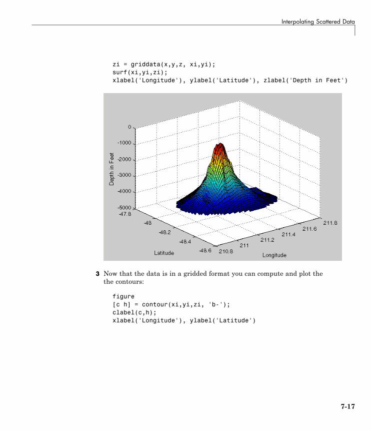
Interpolating Scattered Data
zi = griddata(x,y,z, xi,yi);surf(xi,yi,zi);xlabel('Longitude'), ylabel('Latitude'), zlabel('Depth in Feet')
3 Now that the data is in a gridded format you can compute and plot thethe contours:
figure[c h] = contour(xi,yi,zi, 'b-');clabel(c,h);xlabel('Longitude'), ylabel('Latitude')
7-17
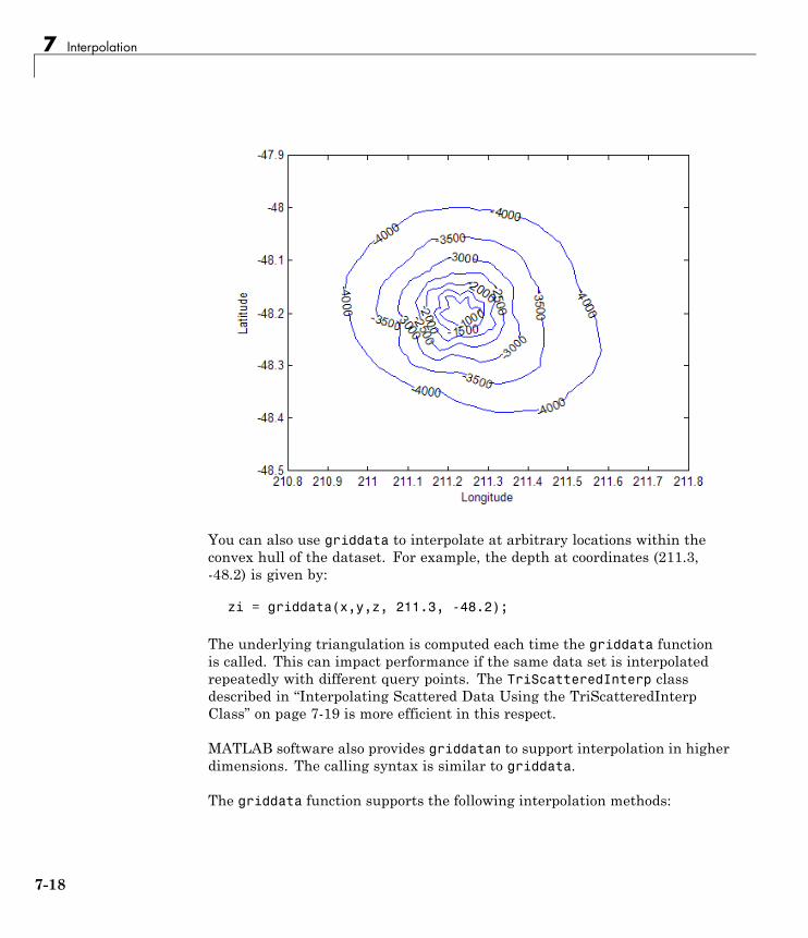
7 Interpolation
You can also use griddata to interpolate at arbitrary locations within theconvex hull of the dataset. For example, the depth at coordinates (211.3,-48.2) is given by:
zi = griddata(x,y,z, 211.3, -48.2);
The underlying triangulation is computed each time the griddata functionis called. This can impact performance if the same data set is interpolatedrepeatedly with different query points. The TriScatteredInterp classdescribed in “Interpolating Scattered Data Using the TriScatteredInterpClass” on page 7-19 is more efficient in this respect.
MATLAB software also provides griddatan to support interpolation in higherdimensions. The calling syntax is similar to griddata.
The griddata function supports the following interpolation methods:
7-18
Interpolating Scattered Data
• 'nearest' — Nearest-neighbor interpolation, where the interpolatingsurface is discontinuous.
• 'linear'— Linear interpolation (default), where the interpolating surfaceis C0 continuous.
• 'cubic' — Cubic interpolation, where the interpolating surface is C2continuous.
The griddatan function supports the following interpolation methods:
• 'nearest' — Nearest-neighbor interpolation, where the interpolatingsurface is discontinuous, and
• 'linear'— Linear interpolation (default), where the interpolating surfaceis C0 continuous.
The 'nearest'and 'linear' methods are computationally more efficientthan the 'cubic' method. The 'cubic' method is generally used whenhigher order continuity of the interpolating function is required. However,'cubic' is not supported by the higher dimensional griddatan function.
Interpolating Scattered Data Using theTriScatteredInterp ClassThe griddata function is useful when you need to interpolate to find thevalues at a set of predefined grid-point locations. In practice, interpolationproblems are often more general, and the TriScatteredInterp class providesgreater flexibility. The class has the following advantages:
• It produces an interpolating function that can be queried efficiently. Thatis, the underlying triangulation is created once and reused for subsequentqueries.
• The interpolation method can be changed independently of thetriangulation.
• The values at the data points can be changed independently of thetriangulation.
• Data points can be incrementally added to the existing interpolant withouttriggering a complete recomputation. Data points can also be removed and
7-19
7 Interpolation
moved efficiently, provided the number of points edited is small relative tothe total number of sample points.
• It supports natural-neighbor interpolation (which is an improvement overlinear interpolation) and works well with larger data sets that have unevensampling.
TriScatteredInterp provides the following interpolation methods:
• 'nearest' — Nearest-neighbor interpolation, where the interpolatingsurface is discontinuous.
• 'linear'— Linear interpolation (default), where the interpolating surfaceis C0 continuous.
• 'natural' — Natural-neighbor interpolation, where the interpolatingsurface is C1 continuous except at the sample points.
The TriScatteredInterp class supports scattered data interpolationin 2-D and 3-D space. You can create the interpolant by calling theTriScatteredInterp constructor and passing the point locations andcorresponding values, and optionally the interpolation method. The pointlocations can be expressed in terms of individual coordinate vectors (x,y), (x, y,z), or as an m-by-n matrix X, where m is the number of points and n the numberof dimensions (2 or 3). Typical calling syntaxes have the following forms.
1 x, y, and v are Mx1 vectors, where M is the number of sample points. Thiscreates a 2-D interpolant.
F = TriScatteredInterp(x,y,v)
2 x, y, z, and v are Mx1 vectors. This creates a 3-D interpolant
F = TriScatteredInterp(x,y,z,v)
3 X is a Mx2 or Mx3 matrix, where M is the number of sample points. Thiscreates a 2-D or 3-D interpolant respectively.
F = TriScatteredInterp(X,V)
4 You can also specify an interpolation method when constructing theinterpolant. This example specifies natural-neighbor interpolation.
7-20
Interpolating Scattered Data
F = TriScatteredInterp(x,y,v, `natural')
You can also construct a TriScatteredInterp from a DelaunayTritriangulation. This method provides more control over the interpolatingtriangulation. This approach is useful for querying the triangulation with aview to adjusting data, removing outliers, or diagnosing anomalies in theinterpolation. See “Addressing Problems in Scattered Data Interpolation”on page 7-32 for further information.
The TriScatteredInterp interpolant is evaluated the same way asevaluating a function.
For example, you can evaluate a 2-D interpolant at the query locations definedby Xq, Yq. You return the computed values in Vq:
Vq = F(Xq, Yq);
Similarly, you can express the query points as an M-by-2 matrix Xq andreturn the computed values in Vq:
Vq = F(Xq);
You can evaluate a 3-D interpolant at the query locations defined by Xq, Yq,Zq, :
Vq = F(Xq, Yq, Zq)
Similarly, you can express the query points as an M-by-3 matrix Xq andreturn the computed values in Vq:
Vq = F(Xq);
Refer to the function reference pages for further information on theconstructor and calling syntax for TriScatteredInterp.
Using TriScatteredInterp features is best demonstrated with this example,which uses the gallery and peaks functions to generate a scattered data set.
1 Create the scattered data set:
X = -3 + 6.*gallery('uniformdata',[250 2],0);V = peaks(X(:,1),X(:,2));
7-21
7 Interpolation
2 Create the interpolant:
F = TriScatteredInterp(X,V)
When MATLAB creates the TriScatteredInterp, it outputs the following:
F =
TriScatteredInterp
Properties:X: [250x2 double]V: [250x1 double]
Method: 'linear'
The X property represents the coordinates of the data points and the Vproperty represents the associated values. The Method property representsthe interpolation method that performs the interpolation. Get help byclicking the TriScatteredInterp or typinghelp TriScatteredInterp.
You can access the properties the same way as for a Struct:
F.X % Gives us the point locationsF.V % Gives the accompanying valuesF.Method % Gives the interpolation method
3 Evaluate the interpolant.
TriScatteredInterp provides subscripted evaluation of the interpolant. Itis evaluated the same way as a function. You can evaluate the interpolantas follows. In this case, the value at the query location is given by Vq. Youcan evaluate at a single query point:
Vq = F([1.5 1.25])Vq =
1.3966
You can also pass individual coordinates:
Vq = F(1.5, 1.25)
7-22
Interpolating Scattered Data
Vq =
1.3966
You can evaluate at a vector of point locations:
Xq = [0.5 0.25; 0.75 0.35; 1.25 0.85]Vq = F(Xq) % Or, you could call with F(Xq(:,1), Xq(:,2))
Vq =1.08801.81272.3472
You can evaluate at grid-point locations followed by a plot:
[Xq Yq] = meshgrid(-2.5:0.125:2.5);Vq = F(Xq, Yq);surf(Xq, Yq, Vq);xlabel('X', 'fontweight','b'), ylabel('Y','fontweight','b')zlabel('Value - V', 'fontweight','b')title('Linear Interpolation Method', 'fontweight','b')
7-23
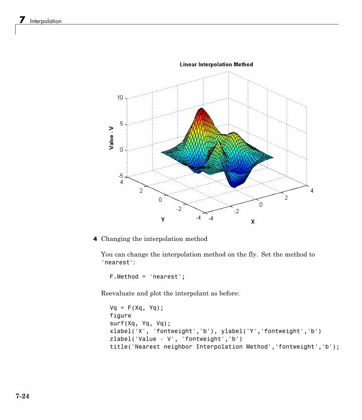
7 Interpolation
4 Changing the interpolation method
You can change the interpolation method on the fly. Set the method to'nearest':
F.Method = 'nearest';
Reevaluate and plot the interpolant as before:
Vq = F(Xq, Yq);figuresurf(Xq, Yq, Vq);xlabel('X', 'fontweight','b'), ylabel('Y','fontweight','b')zlabel('Value - V', 'fontweight','b')title('Nearest neighbor Interpolation Method','fontweight','b');
7-24
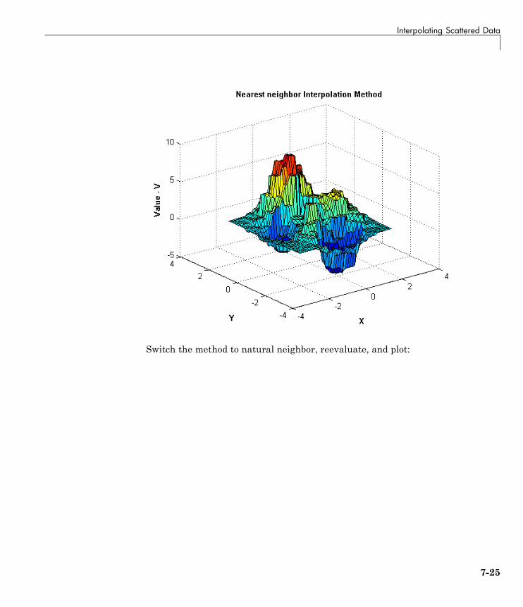
Interpolating Scattered Data
Switch the method to natural neighbor, reevaluate, and plot:
7-25
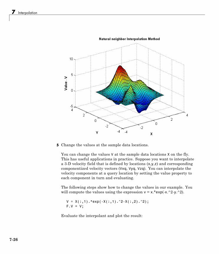
7 Interpolation
5 Change the values at the sample data locations.
You can change the values V at the sample data locations X on the fly.This has useful applications in practice. Suppose you want to interpolatea 3-D velocity field that is defined by locations (x,y,z) and correspondingcomponentized velocity vectors (Vxq, Vyq, Vzq). You can interpolate thevelocity components at a query location by setting the value property toeach component in turn and evaluating.
The following steps show how to change the values in our example. Youwill compute the values using the expression v = x.*exp(-x.^2-y.^2).
V = X(:,1).*exp(-X(:,1).^2-X(:,2).^2);F.V = V;
Evaluate the interpolant and plot the result:
7-26
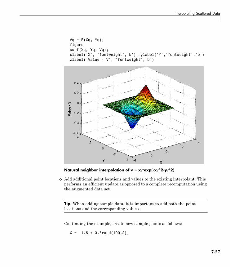
Interpolating Scattered Data
Vq = F(Xq, Yq);figuresurf(Xq, Yq, Vq);xlabel('X', 'fontweight','b'), ylabel('Y','fontweight','b')zlabel('Value - V', 'fontweight','b')
Natural neighbor interpolation of v = x.*exp(-x.^2-y.^2)
6 Add additional point locations and values to the existing interpolant. Thisperforms an efficient update as opposed to a complete recomputation usingthe augmented data set.
Tip When adding sample data, it is important to add both the pointlocations and the corresponding values.
Continuing the example, create new sample points as follows:
X = -1.5 + 3.*rand(100,2);
7-27
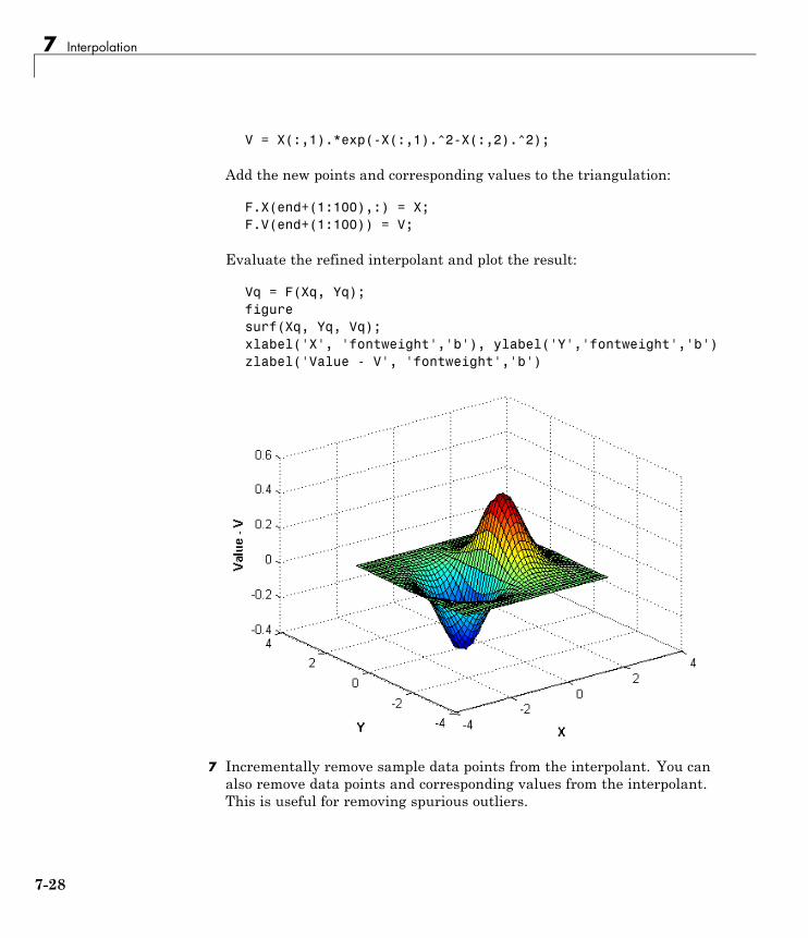
7 Interpolation
V = X(:,1).*exp(-X(:,1).^2-X(:,2).^2);
Add the new points and corresponding values to the triangulation:
F.X(end+(1:100),:) = X;F.V(end+(1:100)) = V;
Evaluate the refined interpolant and plot the result:
Vq = F(Xq, Yq);figuresurf(Xq, Yq, Vq);xlabel('X', 'fontweight','b'), ylabel('Y','fontweight','b')zlabel('Value - V', 'fontweight','b')
7 Incrementally remove sample data points from the interpolant. You canalso remove data points and corresponding values from the interpolant.This is useful for removing spurious outliers.
7-28
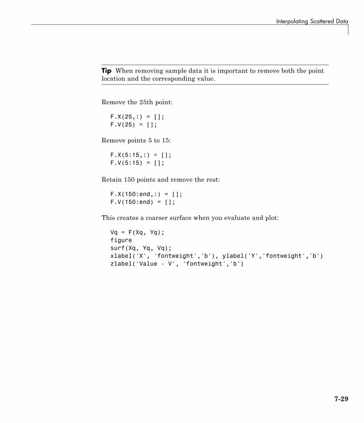
Interpolating Scattered Data
Tip When removing sample data it is important to remove both the pointlocation and the corresponding value.
Remove the 25th point:
F.X(25,:) = [];F.V(25) = [];
Remove points 5 to 15:
F.X(5:15,:) = [];F.V(5:15) = [];
Retain 150 points and remove the rest:
F.X(150:end,:) = [];F.V(150:end) = [];
This creates a coarser surface when you evaluate and plot:
Vq = F(Xq, Yq);figuresurf(Xq, Yq, Vq);xlabel('X', 'fontweight','b'), ylabel('Y','fontweight','b')zlabel('Value - V', 'fontweight','b')
7-29
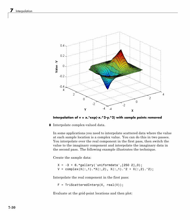
7 Interpolation
Interpolation of v = x.*exp(-x.^2-y.^2) with sample points removed
8 Interpolate complex-valued data.
In some applications you need to interpolate scattered data where the valueat each sample location is a complex value. You can do this in two passes.You interpolate over the real component in the first pass, then switch thevalue to the imaginary component and interpolate the imaginary data inthe second pass. The following example illustrates the technique.
Create the sample data:
X = -3 + 6.*gallery('uniformdata',[250 2],0);V = complex(X(:,1).*X(:,2), X(:,1).^2 + X(:,2).^2);
Interpolate the real component in the first pass:
F = TriScatteredInterp(X, real(V));
Evaluate at the grid-point locations and then plot:
7-30
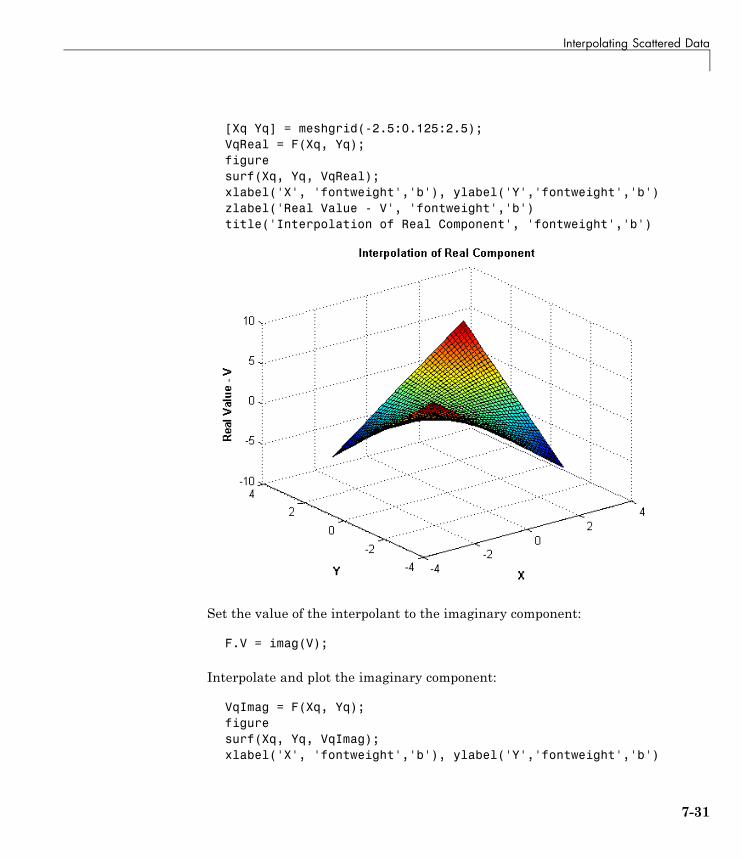
Interpolating Scattered Data
[Xq Yq] = meshgrid(-2.5:0.125:2.5);VqReal = F(Xq, Yq);figuresurf(Xq, Yq, VqReal);xlabel('X', 'fontweight','b'), ylabel('Y','fontweight','b')zlabel('Real Value - V', 'fontweight','b')title('Interpolation of Real Component', 'fontweight','b')
Set the value of the interpolant to the imaginary component:
F.V = imag(V);
Interpolate and plot the imaginary component:
VqImag = F(Xq, Yq);figuresurf(Xq, Yq, VqImag);xlabel('X', 'fontweight','b'), ylabel('Y','fontweight','b')
7-31
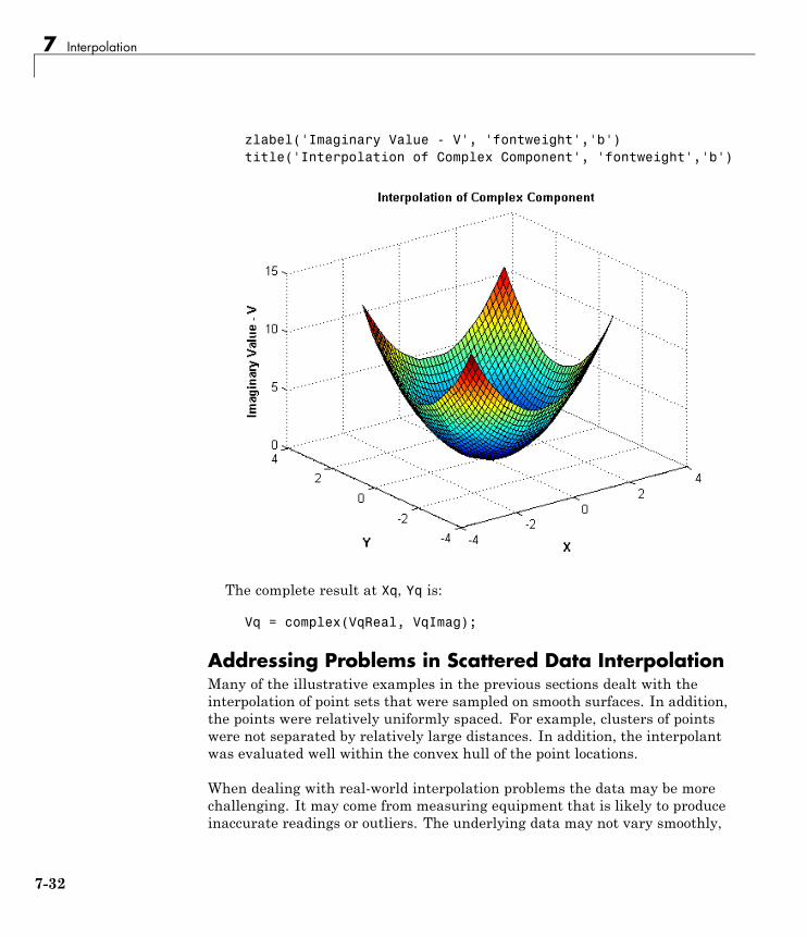
7 Interpolation
zlabel('Imaginary Value - V', 'fontweight','b')title('Interpolation of Complex Component', 'fontweight','b')
The complete result at Xq, Yq is:
Vq = complex(VqReal, VqImag);
Addressing Problems in Scattered Data InterpolationMany of the illustrative examples in the previous sections dealt with theinterpolation of point sets that were sampled on smooth surfaces. In addition,the points were relatively uniformly spaced. For example, clusters of pointswere not separated by relatively large distances. In addition, the interpolantwas evaluated well within the convex hull of the point locations.
When dealing with real-world interpolation problems the data may be morechallenging. It may come from measuring equipment that is likely to produceinaccurate readings or outliers. The underlying data may not vary smoothly,
7-32
Interpolating Scattered Data
the values may jump abruptly from point to point. This section provides youwith some guidelines to identify and address problems with scattered datainterpolation.
Input Data Containing NaNsYou should preprocess sample data that contains NaN values to remove theNaN values as this data cannot contribute to the interpolation. If a NaN isremoved, the corresponding data values/coordinates should also be removedto ensure consistency. If NaN values are present in the sample data, theconstructor will error when called.
The following example illustrates how to remove NaNs.
Create some data and replace some entries with NaN:
x = rand(25,1)*4-2;y = rand(25,1)*4-2;V = x.^2 + y.^2;
x(5) = NaN; x(10) = NaN; y(12) = NaN; V(14) = NaN;
This code errors:
F = TriScatteredInterp(x,y,V)
Instead, find the sample point indices of the NaNs and then construct theinterpolant:
nan_flags = isnan(x) | isnan(y) | isnan(V);
x(nan_flags) = [];y(nan_flags) = [];V(nan_flags) = [];
F = TriScatteredInterp(x,y,V)
The following example is similar if the point locations are in matrix form.First, create data and replace some entries with NaNs:
X = rand(25,2)*4-2;V = X(:,1).^2 + X(:,2).^2;
7-33
7 Interpolation
X(5,1) = NaN; X(10,1) = NaN; X(12,2) = NaN; V(14) = NaN;
This code errors:
F = TriScatteredInterp(X,V)
Find the sample point indices of the NaN and then construct the interpolant:
nan_flags = isnan(X(:,1)) | isnan(X(:,2)) | isnan(V);
X(nan_flags,:) = [];V(nan_flags) = [];
F = TriScatteredInterp(X,V)
Interpolant Outputs NaN ValuesThe linear and natural-neighbor interpolation methods produce an interpolantthat is valid within the convex hull of the point locations. The 'nearest'method does not have a restricted domain as a nearest neighbor to a querypoint always exists. An interpolant that uses the 'linear' or 'natural'method will return NaN values when evaluated at a query point outside theconvex hull. These methods do not perform extrapolation outside of the convexhull of the point locations. However, you can identify such points and assigna value or reevaluate the interpolant using the 'nearest' method to get arepresentative value at that location. The following example demonstratesthis approach.
Create some sample data that lies on the surface of a paraboloid:
x = rand(100,1)*6-3;y = rand(100,1)*6-3;V = x.^2 + y.^2;
The sample point locations are in the range –2 ≤ (x,y) ≤ 2. You can computeand plot the convex hull to get a clearer picture of the supported domain for'linear' and 'natural' interpolation.
plot(x,y, '.');k = convhull(x,y)
7-34
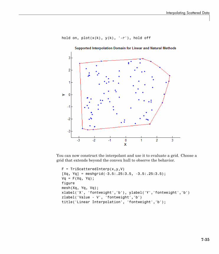
Interpolating Scattered Data
hold on, plot(x(k), y(k), '-r'), hold off
You can now construct the interpolant and use it to evaluate a grid. Choose agrid that extends beyond the convex hull to observe the behavior.
F = TriScatteredInterp(x,y,V)[Xq, Yq] = meshgrid(-3.5:.25:3.5, -3.5:.25:3.5);Vq = F(Xq, Yq);figuremesh(Xq, Yq, Vq);xlabel('X', 'fontweight','b'), ylabel('Y','fontweight','b')zlabel('Value - V', 'fontweight','b')title('Linear Interpolation', 'fontweight','b');
7-35
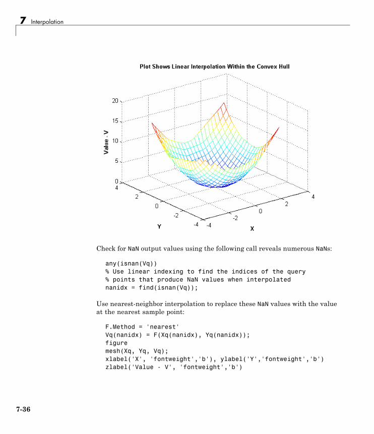
7 Interpolation
Check for NaN output values using the following call reveals numerous NaNs:
any(isnan(Vq))% Use linear indexing to find the indices of the query% points that produce NaN values when interpolatednanidx = find(isnan(Vq));
Use nearest-neighbor interpolation to replace these NaN values with the valueat the nearest sample point:
F.Method = 'nearest'Vq(nanidx) = F(Xq(nanidx), Yq(nanidx));figuremesh(Xq, Yq, Vq);xlabel('X', 'fontweight','b'), ylabel('Y','fontweight','b')zlabel('Value - V', 'fontweight','b')
7-36
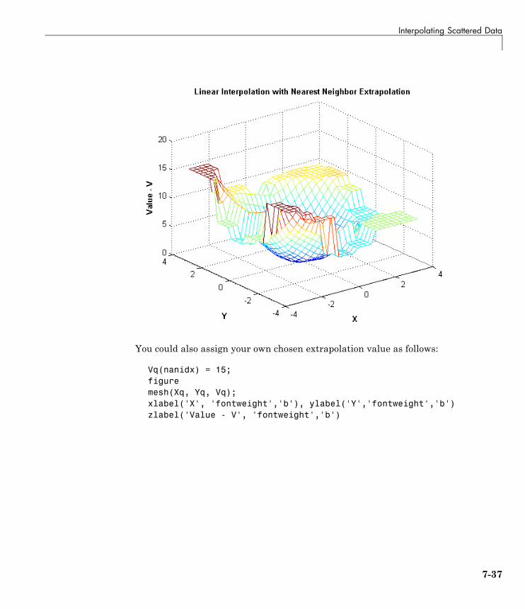
Interpolating Scattered Data
You could also assign your own chosen extrapolation value as follows:
Vq(nanidx) = 15;figuremesh(Xq, Yq, Vq);xlabel('X', 'fontweight','b'), ylabel('Y','fontweight','b')zlabel('Value - V', 'fontweight','b')
7-37
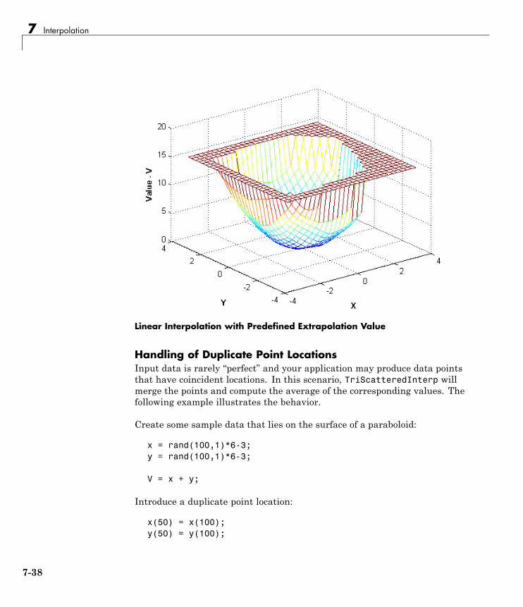
7 Interpolation
Linear Interpolation with Predefined Extrapolation Value
Handling of Duplicate Point LocationsInput data is rarely “perfect” and your application may produce data pointsthat have coincident locations. In this scenario, TriScatteredInterp willmerge the points and compute the average of the corresponding values. Thefollowing example illustrates the behavior.
Create some sample data that lies on the surface of a paraboloid:
x = rand(100,1)*6-3;y = rand(100,1)*6-3;
V = x + y;
Introduce a duplicate point location:
x(50) = x(100);y(50) = y(100);
7-38
Interpolating Scattered Data
Create the interpolation:
F = TriScatteredInterp(x,y,V)F.V(50)
(V(50)+V(100))/2
In this scenario the interpolant resolves the ambiguity in a reasonablemanner. However, in some instances data points may be close rather thancoincident, and the values at those locations may be very different.
Interpolation Results Poor Near the Convex HullThe Delaunay triangulation is well suited to scattered data interpolationproblems because it has favorable geometric properties that produce goodresults. Namely the rejection of sliver-shaped triangles/tetrahedra in favorof more equilateral-shaped ones, and the empty circumcircle property thatimplicitly defines a nearest-neighbor relation between the points. This latterproperty ensures the interpolated values are influenced by sample pointsin the neighborhood of the query location. Despite these qualities, in somesituations the distribution of the data points may lead to poor results andthis typically happens near the convex hull of the sample data set. Whenthe interpolation produces unexpected results, a plot of the sample data andunderlying triangulation can often provide insight into the problem. Thefollowing example illustrates such behavior.
Create a sample data set that will exhibit problems near the boundary :
t = 0.4*pi:0.02:0.6*pi;x1 = cos(t)';y1 = sin(t)'-1.02;x2 = x1;y2 = y1*(-1);x3 = linspace(-0.3,0.3,16)';y3 = zeros(16,1);x = [x1;x2;x3];y = [y1;y2;y3];
Now lift these sample points onto the surface z = x.^2 + y.^2 and interpolatethe surface.
7-39
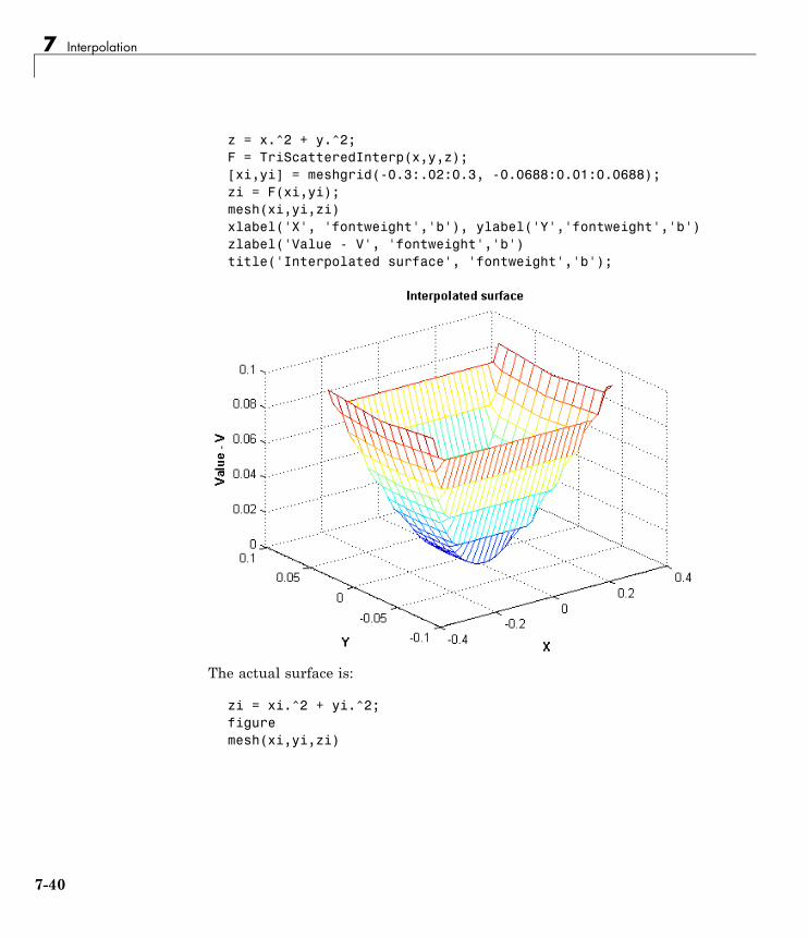
7 Interpolation
z = x.^2 + y.^2;F = TriScatteredInterp(x,y,z);[xi,yi] = meshgrid(-0.3:.02:0.3, -0.0688:0.01:0.0688);zi = F(xi,yi);mesh(xi,yi,zi)xlabel('X', 'fontweight','b'), ylabel('Y','fontweight','b')zlabel('Value - V', 'fontweight','b')title('Interpolated surface', 'fontweight','b');
The actual surface is:
zi = xi.^2 + yi.^2;figuremesh(xi,yi,zi)
7-40
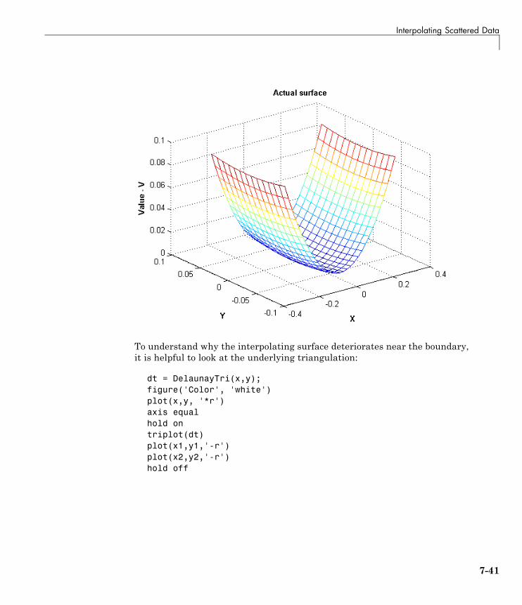
Interpolating Scattered Data
To understand why the interpolating surface deteriorates near the boundary,it is helpful to look at the underlying triangulation:
dt = DelaunayTri(x,y);figure('Color', 'white')plot(x,y, '*r')axis equalhold ontriplot(dt)plot(x1,y1,'-r')plot(x2,y2,'-r')hold off
7-41
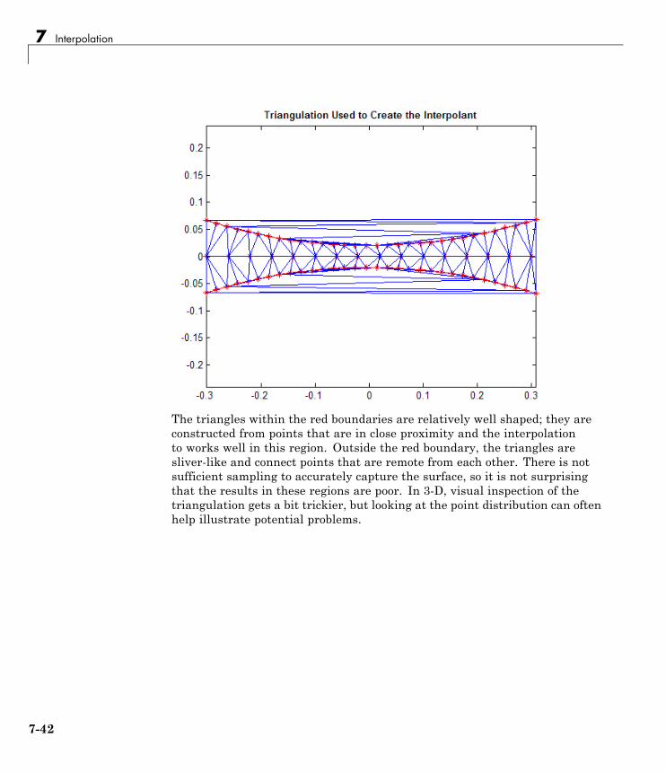
7 Interpolation
The triangles within the red boundaries are relatively well shaped; they areconstructed from points that are in close proximity and the interpolationto works well in this region. Outside the red boundary, the triangles aresliver-like and connect points that are remote from each other. There is notsufficient sampling to accurately capture the surface, so it is not surprisingthat the results in these regions are poor. In 3-D, visual inspection of thetriangulation gets a bit trickier, but looking at the point distribution can oftenhelp illustrate potential problems.
7-42
8
Optimization
• “Function Summary” on page 8-2
• “Optimizing Nonlinear Functions” on page 8-3
• “Example: Curve Fitting via Optimization” on page 8-9
• “Setting Options” on page 8-12
• “Iterative Display” on page 8-14
• “Output Functions” on page 8-16
• “Plot Functions” on page 8-24
• “Troubleshooting and Tips” on page 8-27
• “Reference” on page 8-29

8 Optimization
Function SummaryThe following table lists the MATLAB optimization functions.
Function Description
fminbnd Minimize a function of one variable on a fixedinterval
fminsearch Minimize a function of several variables
fzero Find zero of a function of one variable
lsqnonneg Linear least squares with nonnegativityconstraints
optimget Get optimization options structure parametervalues
optimset Create or edit optimization options parameterstructure
To maximize a function, see “Maximizing Functions” on page 8-7. Forinformation on solving single-variable nonlinear equations, see “Roots ofScalar Functions” on page 5-6.
For more optimization capabilities, see the Optimization Toolbox™ User’sGuide.
8-2
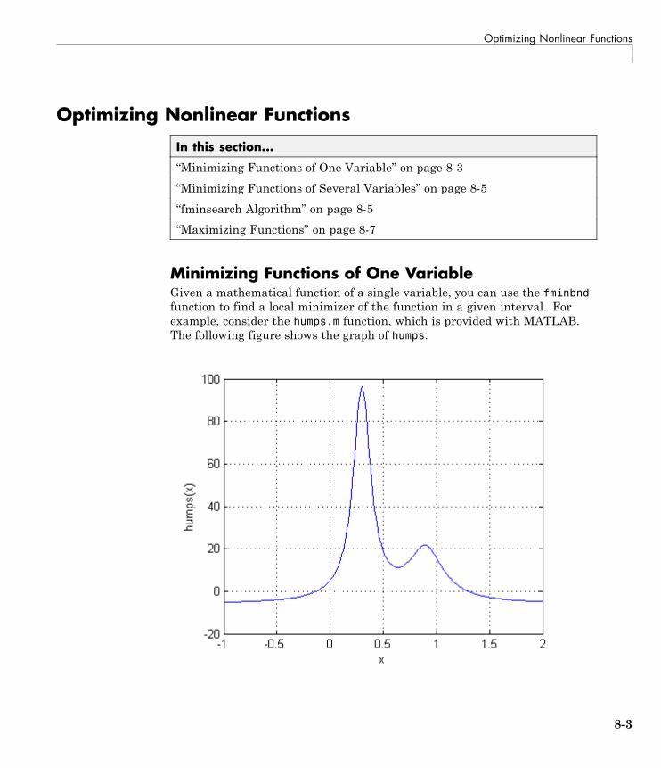
Optimizing Nonlinear Functions
Optimizing Nonlinear Functions
In this section...
“Minimizing Functions of One Variable” on page 8-3
“Minimizing Functions of Several Variables” on page 8-5
“fminsearch Algorithm” on page 8-5
“Maximizing Functions” on page 8-7
Minimizing Functions of One VariableGiven a mathematical function of a single variable, you can use the fminbndfunction to find a local minimizer of the function in a given interval. Forexample, consider the humps.m function, which is provided with MATLAB.The following figure shows the graph of humps.
8-3
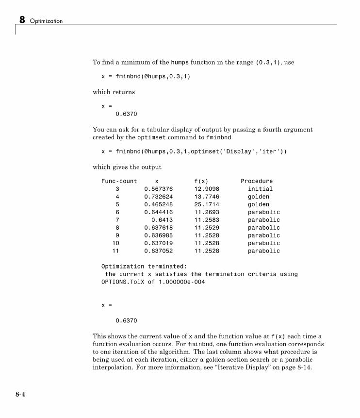
8 Optimization
To find a minimum of the humps function in the range (0.3,1), use
x = fminbnd(@humps,0.3,1)
which returns
x =0.6370
You can ask for a tabular display of output by passing a fourth argumentcreated by the optimset command to fminbnd
x = fminbnd(@humps,0.3,1,optimset('Display','iter'))
which gives the output
Func-count x f(x) Procedure3 0.567376 12.9098 initial4 0.732624 13.7746 golden5 0.465248 25.1714 golden6 0.644416 11.2693 parabolic7 0.6413 11.2583 parabolic8 0.637618 11.2529 parabolic9 0.636985 11.2528 parabolic
10 0.637019 11.2528 parabolic11 0.637052 11.2528 parabolic
Optimization terminated:the current x satisfies the termination criteria using
OPTIONS.TolX of 1.000000e-004
x =
0.6370
This shows the current value of x and the function value at f(x) each time afunction evaluation occurs. For fminbnd, one function evaluation correspondsto one iteration of the algorithm. The last column shows what procedure isbeing used at each iteration, either a golden section search or a parabolicinterpolation. For more information, see “Iterative Display” on page 8-14.
8-4
Optimizing Nonlinear Functions
Minimizing Functions of Several VariablesThe fminsearch function is similar to fminbnd except that it handlesfunctions of many variables, and you specify a starting vector x0 rather thana starting interval. fminsearch attempts to return a vector x that is a localminimizer of the mathematical function near this starting vector.
To try fminsearch, create a function three_var of three variables, x, y, and z.
function b = three_var(v)x = v(1);y = v(2);z = v(3);b = x.^2 + 2.5*sin(y) - z^2*x^2*y^2;
Now find a minimum for this function using x = -0.6, y = -1.2, andz = 0.135 as the starting values.
v = [-0.6 -1.2 0.135];a = fminsearch(@three_var,v)
a =0.0000 -1.5708 0.1803
fminsearch Algorithmfminsearch uses the Nelder-Mead simplex algorithm as described in Lagariaset al. [1]. This algorithm uses a simplex of n + 1 points for n-dimensionalvectors x. The algorithm first makes a simplex around the initial guess x0by adding 5% of each component x0(i) to x0, and using these n vectors aselements of the simplex in addition to x0. (It uses 0.00025 as component i ifx0(i) = 0.) Then, the algorithm modifies the simplex repeatedly accordingto the following procedure.
Note The keywords for the fminsearch iterative display appear in bold afterthe description of the step.
1 Let x(i) denote the list of points in the current simplex, i = 1,...,n+1.
8-5
8 Optimization
2 Order the points in the simplex from lowest function value f(x(1)) tohighest f(x(n+1)). At each step in the iteration, the algorithm discards thecurrent worst point x(n+1), and accepts another point into the simplex. [Or,in the case of step 7 below, it changes all n points with values above f(x(1))].
3 Generate the reflected point
r = 2m – x(n+1),
where
m = Σx(i)/n, i = 1...n,
and calculate f(r).
4 If f(x(1)) ≤ f(r) < f(x(n)), accept r and terminate this iteration. Reflect
5 If f(r) < f(x(1)), calculate the expansion point s
s = m + 2(m – x(n+1)),
and calculate f(s).
a If f(s) < f(r), accept s and terminate the iteration. Expand
b Otherwise, accept r and terminate the iteration. Reflect
6 If f(r) ≥ f(x(n)), perform a contraction between m and the better of x(n+1)and r:
a If f(r) < f(x(n+1)) (i.e., r is better than x(n+1)), calculate
c = m + (r – m)/2
and calculate f(c). If f(c) < f(r), accept c and terminate the iteration.Contract outside Otherwise, continue with Step 7 (Shrink).
b If f(r) ≥ f(x(n+1)), calculate
cc = m + (x(n+1) – m)/2
and calculate f(cc). If f(cc) < f(x(n+1)), accept cc and terminate theiteration. Contract inside Otherwise, continue with Step 7 (Shrink).
8-6
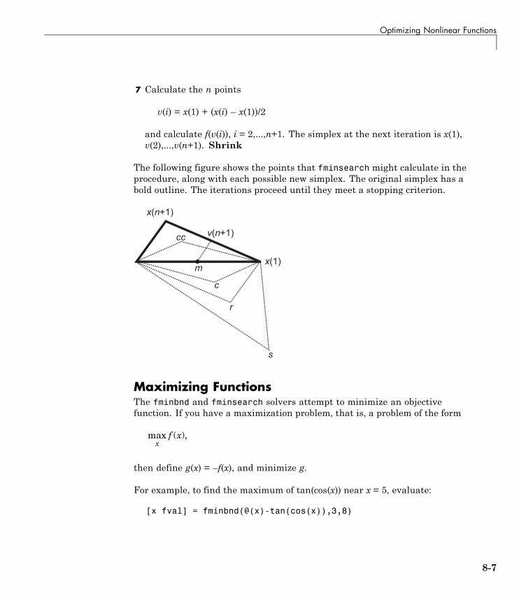
Optimizing Nonlinear Functions
7 Calculate the n points
v(i) = x(1) + (x(i) – x(1))/2
and calculate f(v(i)), i = 2,...,n+1. The simplex at the next iteration is x(1),v(2),...,v(n+1). Shrink
The following figure shows the points that fminsearch might calculate in theprocedure, along with each possible new simplex. The original simplex has abold outline. The iterations proceed until they meet a stopping criterion.
�
������
�
����
������
�
�
��
Maximizing FunctionsThe fminbnd and fminsearch solvers attempt to minimize an objectivefunction. If you have a maximization problem, that is, a problem of the form
max ( ),x
f x
then define g(x) = –f(x), and minimize g.
For example, to find the maximum of tan(cos(x)) near x = 5, evaluate:
[x fval] = fminbnd(@(x)-tan(cos(x)),3,8)
8-7
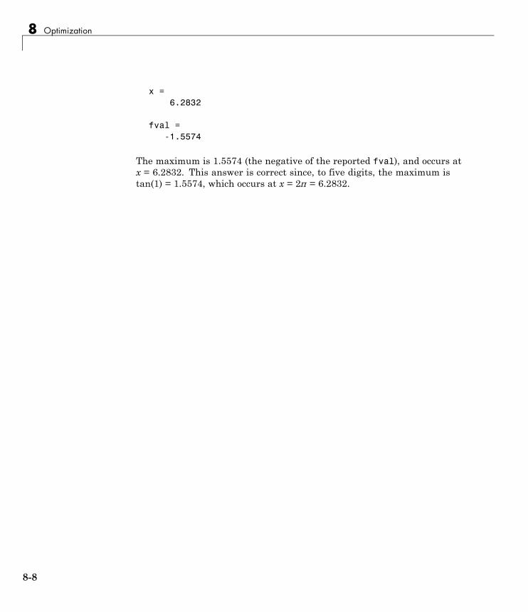
8 Optimization
x =6.2832
fval =-1.5574
The maximum is 1.5574 (the negative of the reported fval), and occurs atx = 6.2832. This answer is correct since, to five digits, the maximum istan(1) = 1.5574, which occurs at x = 2π = 6.2832.
8-8
Example: Curve Fitting via Optimization
Example: Curve Fitting via Optimization
In this section...
“Curve Fitting by Optimization” on page 8-9
“Creating an Example File” on page 8-9
“Running the Example” on page 8-10
“Plotting the Results” on page 8-10
Curve Fitting by OptimizationThis section gives an example that shows how to fit an exponential functionof the form Ae–λt to some data. The example uses the fminsearch solver tominimize the sum of squares of errors between the data and an exponentialfunction Ae–λt for varying parameters A and λ.
Creating an Example FileTo run the example, first create a file that:
• Accepts vectors corresponding to the x- and y-coordinates of the data
• Returns the parameters of the exponential function that best fits the data
To do so, copy and paste the following code into a file and save it asfitcurvedemo in a directory on the MATLAB path.
function [estimates, model] = fitcurvedemo(xdata, ydata)% Call fminsearch with a random starting point.start_point = rand(1, 2);model = @expfun;estimates = fminsearch(model, start_point);% expfun accepts curve parameters as inputs, and outputs sse,% the sum of squares error for A*exp(-lambda*xdata)-ydata,% and the FittedCurve. FMINSEARCH only needs sse, but we want% to plot the FittedCurve at the end.
function [sse, FittedCurve] = expfun(params)A = params(1);lambda = params(2);
8-9
8 Optimization
FittedCurve = A .* exp(-lambda * xdata);ErrorVector = FittedCurve - ydata;sse = sum(ErrorVector .^ 2);
endend
The file calls the function fminsearch, which finds parameters A and lambdathat minimize the sum of squares of the differences between the data andthe exponential function A*exp(-lambda*t). The nested function expfuncomputes the sum of squares.
Running the ExampleTo run the example, first create some random data to fit. The followingcommands create random data that is approximately exponential withparameters A = 40 and lambda = .5.
xdata = (0:.1:10)';ydata = 40 * exp(-.5 * xdata) + randn(size(xdata));
To fit an exponential function to the data, enter
[estimates, model] = fitcurvedemo(xdata,ydata)
This returns estimates for the parameters A and lambda,
estimates =
40.1334 0.5025
and a function handle, model, to the function that computes the exponentialfunction A*exp(-lambda*t).
Plotting the ResultsTo plot the fit and the data, enter the following commands.
plot(xdata, ydata, '*')hold on[sse, FittedCurve] = model(estimates);plot(xdata, FittedCurve, 'r')
8-10
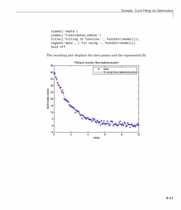
Example: Curve Fitting via Optimization
xlabel('xdata')ylabel('f(estimates,xdata)')title(['Fitting to function ', func2str(model)]);legend('data', ['fit using ', func2str(model)])hold off
The resulting plot displays the data points and the exponential fit.
8-11
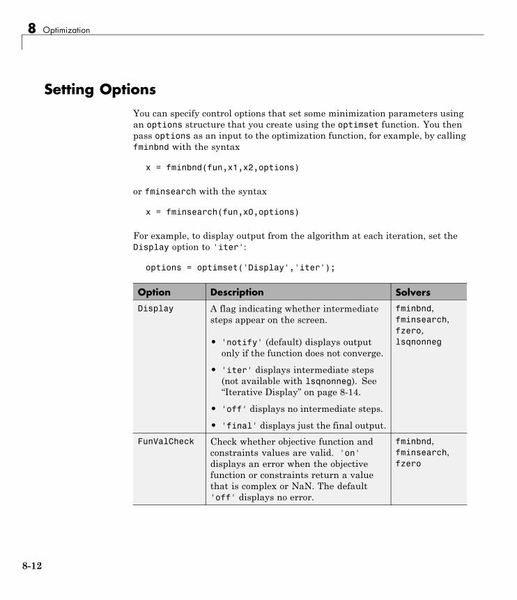
8 Optimization
Setting OptionsYou can specify control options that set some minimization parameters usingan options structure that you create using the optimset function. You thenpass options as an input to the optimization function, for example, by callingfminbnd with the syntax
x = fminbnd(fun,x1,x2,options)
or fminsearch with the syntax
x = fminsearch(fun,x0,options)
For example, to display output from the algorithm at each iteration, set theDisplay option to 'iter':
options = optimset('Display','iter');
Option Description Solvers
Display A flag indicating whether intermediatesteps appear on the screen.
• 'notify' (default) displays outputonly if the function does not converge.
• 'iter' displays intermediate steps(not available with lsqnonneg). See“Iterative Display” on page 8-14.
• 'off' displays no intermediate steps.
• 'final' displays just the final output.
fminbnd,fminsearch,fzero,lsqnonneg
FunValCheck Check whether objective function andconstraints values are valid. 'on'displays an error when the objectivefunction or constraints return a valuethat is complex or NaN. The default'off' displays no error.
fminbnd,fminsearch,fzero
8-12
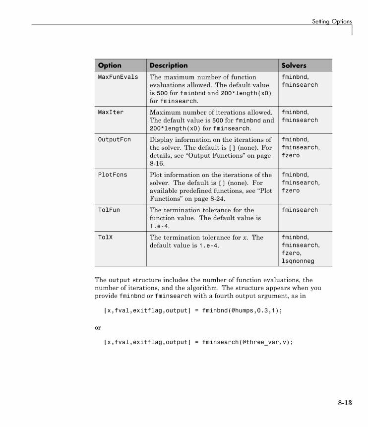
Setting Options
Option Description Solvers
MaxFunEvals The maximum number of functionevaluations allowed. The default valueis 500 for fminbnd and 200*length(x0)for fminsearch.
fminbnd,fminsearch
MaxIter Maximum number of iterations allowed.The default value is 500 for fminbnd and200*length(x0) for fminsearch.
fminbnd,fminsearch
OutputFcn Display information on the iterations ofthe solver. The default is [] (none). Fordetails, see “Output Functions” on page8-16.
fminbnd,fminsearch,fzero
PlotFcns Plot information on the iterations of thesolver. The default is [] (none). Foravailable predefined functions, see “PlotFunctions” on page 8-24.
fminbnd,fminsearch,fzero
TolFun The termination tolerance for thefunction value. The default value is1.e-4.
fminsearch
TolX The termination tolerance for x. Thedefault value is 1.e-4.
fminbnd,fminsearch,fzero,lsqnonneg
The output structure includes the number of function evaluations, thenumber of iterations, and the algorithm. The structure appears when youprovide fminbnd or fminsearch with a fourth output argument, as in
[x,fval,exitflag,output] = fminbnd(@humps,0.3,1);
or
[x,fval,exitflag,output] = fminsearch(@three_var,v);
8-13
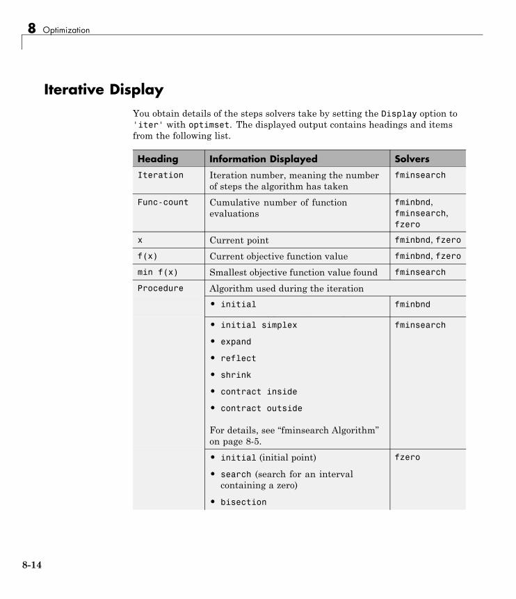
8 Optimization
Iterative DisplayYou obtain details of the steps solvers take by setting the Display option to'iter' with optimset. The displayed output contains headings and itemsfrom the following list.
Heading Information Displayed Solvers
Iteration Iteration number, meaning the numberof steps the algorithm has taken
fminsearch
Func-count Cumulative number of functionevaluations
fminbnd,fminsearch,fzero
x Current point fminbnd, fzero
f(x) Current objective function value fminbnd, fzero
min f(x) Smallest objective function value found fminsearch
Algorithm used during the iteration
• initial
• golden (golden section search)
• parabolic (parabolic interpolation)
fminbnd
• initial simplex
• expand
• reflect
• shrink
• contract inside
• contract outside
For details, see “fminsearch Algorithm”on page 8-5.
fminsearch
Procedure
• initial (initial point)
• search (search for an intervalcontaining a zero)
• bisection
fzero
8-14
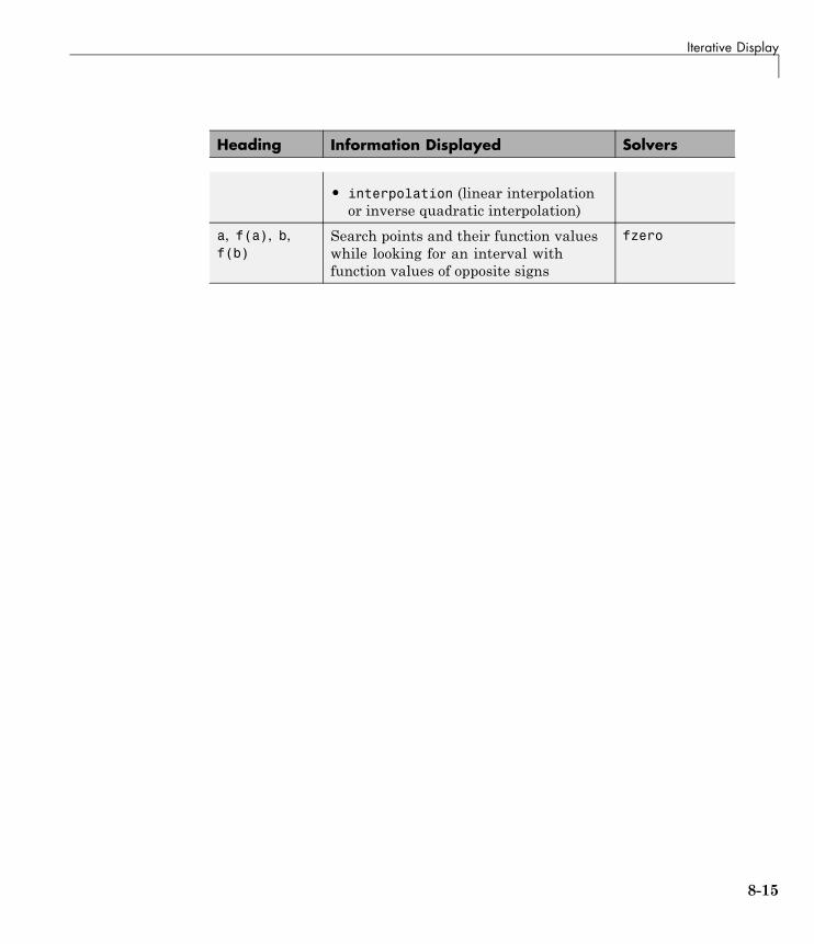
Iterative Display
Heading Information Displayed Solvers
• interpolation (linear interpolationor inverse quadratic interpolation)
a, f(a), b,f(b)
Search points and their function valueswhile looking for an interval withfunction values of opposite signs
fzero
8-15
8 Optimization
Output Functions
In this section...
“What Is an Output Function?” on page 8-16
“Creating and Using an Output Function” on page 8-16
“Structure of the Output Function” on page 8-18
“Example of a Nested Output Function” on page 8-19
“Fields in optimValues” on page 8-21
“States of the Algorithm” on page 8-21
“Stop Flag” on page 8-22
What Is an Output Function?An output function is a function that an optimization function calls at eachiteration of its algorithm. Typically, you might use an output function togenerate graphical output, record the history of the data the algorithmgenerates, or halt the algorithm based on the data at the current iteration.You can create an output function as a function file, a subfunction, or anested function.
You can use the OutputFcn option with the following MATLAB optimizationfunctions:
• fminbnd
• fminsearch
• fzero
Creating and Using an Output FunctionThe following is a simple example of an output function that plots the pointsgenerated by an optimization function.
function stop = outfun(x, optimValues, state)stop = false;hold on;plot(x(1),x(2),'.');
8-16
Output Functions
drawnow
You can use this output function to plot the points generated by fminsearchin solving the optimization problem
min ( ) min .x x
xf x e x x x x x= + + + +( )1 4 2 4 2 112
22
1 2 2
To do so,
1 Create a file containing the preceding code and save it as outfun.m ina directory on the MATLAB path.
2 Enter the command
options = optimset('OutputFcn', @outfun);
to set the value of the Outputfcn field of the options structure to afunction handle to outfun.
3 Enter the following commands:
hold onobjfun=@(x) exp(x(1))*(4*x(1)^2+2*x(2)^2+x(1)*x(2)+2*x(2));[x fval] = fminsearch(objfun, [-1 1], options)hold off
This returns the solution
x =0.1290 -0.5323
fval =-0.5689
and displays the following plot of the points generated by fminsearch:
8-17

8 Optimization
Structure of the Output FunctionThe function definition line of the output function has the following form:
stop = outfun(x, optimValues, state)
where
• stop is a flag that is true or false depending on whether the optimizationroutine should quit or continue. See “Stop Flag” on page 8-22.
• x is the point computed by the algorithm at the current iteration.
• optimValues is a structure containing data from the current iteration.“Fields in optimValues” on page 8-21 describes the structure in detail.
• state is the current state of the algorithm. “States of the Algorithm” onpage 8-21 lists the possible values.
The optimization function passes the values of the input arguments to outfunat each iteration.
8-18
Output Functions
Example of a Nested Output FunctionThe example in “Creating and Using an Output Function” on page 8-16 doesnot require the output function to preserve data from one iteration to the next.When this is the case, you can write the output function as a function file andcall the optimization function directly from the command line. However, ifyou want your output function to record data from one iteration to the next,you should write a single file that does the following:
• Contains the output function as a nested function—see “Nested Functions”in MATLAB Programming Fundamentals for more information.
• Calls the optimization function.
In the following example, the function file also contains the objective functionas a subfunction, although you could also write the objective function as aseparate file or as an anonymous function.
Since the nested function has access to variables in the file that containsit, this method enables the output function to preserve variables from oneiteration to the next.
The following example uses an output function to record the points generatedby fminsearch in solving the optimization problem
min ( ) min .x x
xf x e x x x x x= + + + +( )1 4 2 4 2 112
22
1 2 2
The output function returns the sequence of points as a matrix called history.
To run the example, do the following steps:
1 Open a new file in the MATLAB Editor.
2 Copy and paste the following code into the file.
function [x fval history] = myproblem(x0)history = [];options = optimset('OutputFcn', @myoutput);[x fval] = fminsearch(@objfun, x0,options);
8-19
8 Optimization
function stop = myoutput(x,optimvalues,state);stop = false;if state == 'iter'
history = [history; x];end
end
function z = objfun(x)z = exp(x(1))*(4*x(1)^2+2*x(2)^2+x(1)*x(2)+2*x(2));
endend
3 Save the file as myproblem.m in a directory on the MATLAB path.
4 At the MATLAB prompt, enter
[x fval history] = myproblem([-1 1])
The function fminsearch returns x, the optimal point, and fval, the value ofthe objective function at x.
x =
0.1290 -0.5323
fval =
-0.5689
In addition, the output function myoutput returns the matrix history, whichcontains the points generated by the algorithm at each iteration, to theMATLAB workspace. The first four rows of history are
history(1:4,:) =
-1.0000 1.0000-1.0000 1.0000-1.0750 0.9000-1.0125 0.8500
8-20
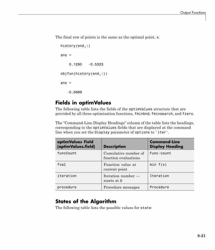
Output Functions
The final row of points is the same as the optimal point, x.
history(end,:)
ans =
0.1290 -0.5323
objfun(history(end,:))
ans =
-0.5689
Fields in optimValuesThe following table lists the fields of the optimValues structure that areprovided by all three optimization functions, fminbnd, fminsearch, and fzero.
The “Command-Line Display Headings” column of the table lists the headings,corresponding to the optimValues fields that are displayed at the commandline when you set the Display parameter of options to 'iter'.
optimValues Field(optimValues.field) Description
Command-LineDisplay Heading
funcCount Cumulative number offunction evaluations
Func-count
fval Function value atcurrent point
min f(x)
iteration Iteration number —starts at 0
Iteration
procedure Procedure messages Procedure
States of the AlgorithmThe following table lists the possible values for state:
8-21
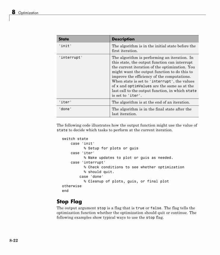
8 Optimization
State Description
'init' The algorithm is in the initial state before thefirst iteration.
'interrupt' The algorithm is performing an iteration. Inthis state, the output function can interruptthe current iteration of the optimization. Youmight want the output function to do this toimprove the efficiency of the computations.When state is set to 'interrupt', the valuesof x and optimValues are the same as at thelast call to the output function, in which stateis set to 'iter'.
'iter' The algorithm is at the end of an iteration.
'done' The algorithm is in the final state after thelast iteration.
The following code illustrates how the output function might use the value ofstate to decide which tasks to perform at the current iteration.
switch statecase 'init'
% Setup for plots or guiscase 'iter'
% Make updates to plot or guis as needed.case 'interrupt'
% Check conditions to see whether optimization% should quit.
case 'done'% Cleanup of plots, guis, or final plot
otherwiseend
Stop FlagThe output argument stop is a flag that is true or false. The flag tells theoptimization function whether the optimization should quit or continue. Thefollowing examples show typical ways to use the stop flag.
8-22
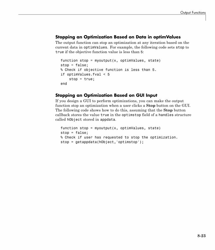
Output Functions
Stopping an Optimization Based on Data in optimValuesThe output function can stop an optimization at any iteration based on thecurrent data in optimValues. For example, the following code sets stop totrue if the objective function value is less than 5:
function stop = myoutput(x, optimValues, state)stop = false;% Check if objective function is less than 5.if optimValues.fval < 5
stop = true;end
Stopping an Optimization Based on GUI InputIf you design a GUI to perform optimizations, you can make the outputfunction stop an optimization when a user clicks a Stop button on the GUI.The following code shows how to do this, assuming that the Stop buttoncallback stores the value true in the optimstop field of a handles structurecalled hObject stored in appdata.
function stop = myoutput(x, optimValues, state)stop = false;% Check if user has requested to stop the optimization.stop = getappdata(hObject,'optimstop');
8-23
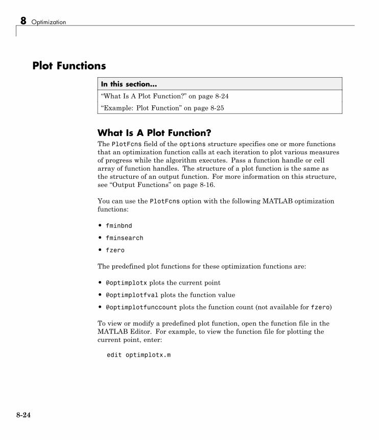
8 Optimization
Plot Functions
In this section...
“What Is A Plot Function?” on page 8-24
“Example: Plot Function” on page 8-25
What Is A Plot Function?The PlotFcns field of the options structure specifies one or more functionsthat an optimization function calls at each iteration to plot various measuresof progress while the algorithm executes. Pass a function handle or cellarray of function handles. The structure of a plot function is the same asthe structure of an output function. For more information on this structure,see “Output Functions” on page 8-16.
You can use the PlotFcns option with the following MATLAB optimizationfunctions:
• fminbnd
• fminsearch
• fzero
The predefined plot functions for these optimization functions are:
• @optimplotx plots the current point
• @optimplotfval plots the function value
• @optimplotfunccount plots the function count (not available for fzero)
To view or modify a predefined plot function, open the function file in theMATLAB Editor. For example, to view the function file for plotting thecurrent point, enter:
edit optimplotx.m
8-24

Plot Functions
Example: Plot FunctionView the progress of a minimization using fminsearch with the plot function@optimplotfval:
1 Write a file for the objective function. For this example, use:
function f = onehump(x)
r = x(1)^2 + x(2)^2;s = exp(-r);f = x(1)*s+r/20;
2 Set the options to use the plot function:
options = optimset('PlotFcns',@optimplotfval);
3 Call fminsearch starting from [2,1]:
[x ffinal] = fminsearch(@onehump,[2,1],options)
4 MATLAB returns the following:
x =-0.6691 0.0000
ffinal =-0.4052
8-25
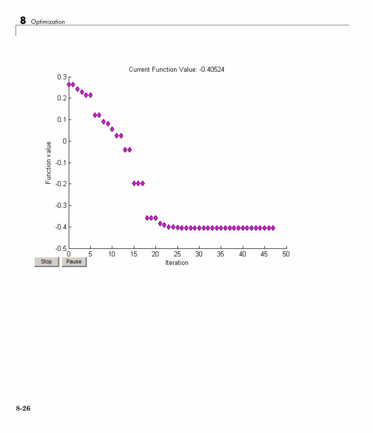
8 Optimization
8-26
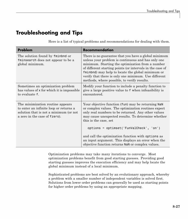
Troubleshooting and Tips
Troubleshooting and TipsHere is a list of typical problems and recommendations for dealing with them.
Problem Recommendation
The solution found by fminbnd orfminsearch does not appear to be aglobal minimum.
There is no guarantee that you have a global minimumunless your problem is continuous and has only oneminimum. Starting the optimization from a numberof different starting points (or intervals in the case offminbnd) may help to locate the global minimum orverify that there is only one minimum. Use differentmethods, where possible, to verify results.
Sometimes an optimization problemhas values of x for which it is impossibleto evaluate f.
Modify your function to include a penalty function togive a large positive value to f when infeasibility isencountered.
The minimization routine appearsto enter an infinite loop or returns asolution that is not a minimum (or nota zero in the case of fzero).
Your objective function (fun) may be returning NaNor complex values. The optimization routines expectonly real numbers to be returned. Any other valuesmay cause unexpected results. To determine whetherthis is the case, set
options = optimset('FunValCheck', 'on')
and call the optimization function with options asan input argument. This displays an error when theobjective function returns NaN or complex values.
Optimization problems may take many iterations to converge. Mostoptimization problems benefit from good starting guesses. Providing goodstarting guesses improves the execution efficiency and may help locate theglobal minimum instead of a local minimum.
Sophisticated problems are best solved by an evolutionary approach, wherebya problem with a smaller number of independent variables is solved first.Solutions from lower order problems can generally be used as starting pointsfor higher order problems by using an appropriate mapping.
8-27

8 Optimization
The use of simpler cost functions and less stringent termination criteria in theearly stages of an optimization problem can also reduce computation time.Such an approach often produces superior results by avoiding local minima.
8-28
Reference
Reference[1] Lagarias, J. C., J. A. Reeds, M. H. Wright, and P. E. Wright. “ConvergenceProperties of the Nelder-Mead Simplex Method in Low Dimensions.” SIAMJournal of Optimization, Vol. 9, Number 1, 1998, pp. 112–147.
8-29

8 Optimization
8-30

9
Function Handles
• “Introduction” on page 9-2
• “Defining Functions In Files” on page 9-3
• “Anonymous Functions” on page 9-4
• “Example: Function Plotting Function” on page 9-5
• “Parameterizing Functions” on page 9-8
9 Function Handles
IntroductionMATLAB functions are written to named files or are produced at thecommand line as anonymous functions. In either case, a function handle isused to pass the function as an input argument to a function function.
9-2
Defining Functions In Files
Defining Functions In FilesConsider the example function:
f xx x
( )( . ) . ( . ) .
.=− +
+− +
−1
0 3 0 01
1
0 9 0 046
2 2
A file for the function is humps.m. Its contents look like this:
function y = humps(x)y = 1./((x - 0.3).^2 + 0.01) ...
+ 1./((x - 0.9).^2 + 0.04) - 6;
To evaluate humps at 2.0, first use @ to obtain a function handle. Use thefunction handle in the same way you would use a function name to call afunction:
fh = @humps;fh(2.0)ans =
-4.8552
9-3
9 Function Handles
Anonymous FunctionsConsider again the example function:
f xx x
( )( . ) . ( . ) .
.=− +
+− +
−1
0 3 0 01
1
0 9 0 046
2 2
A second way to represent the function in the MATLAB is to create ananonymous function at the command line, as follows:
fh = @(x)(1./((x-0.3).^2 + 0.01) ...+ 1./((x-0.9).^2 + 0.04)-6);
You evaluate fh at 2.0 the same way you do with a function handle for afile-defined function:
fh(2.0)ans =
-4.8552
Anonymous functions can have any number of arguments. The followinganonymous function has two input arguments x and y:
fh = @(x,y)(y*sin(x)+x*cos(y));fh(pi,2*pi)ans =
3.1416
9-4
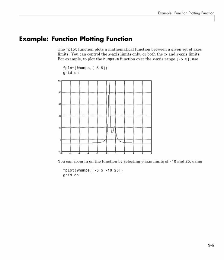
Example: Function Plotting Function
Example: Function Plotting FunctionThe fplot function plots a mathematical function between a given set of axeslimits. You can control the x-axis limits only, or both the x- and y-axis limits.For example, to plot the humps.m function over the x-axis range [-5 5], use
fplot(@humps,[-5 5])grid on
You can zoom in on the function by selecting y-axis limits of -10 and 25, using
fplot(@humps,[-5 5 -10 25])grid on
9-5
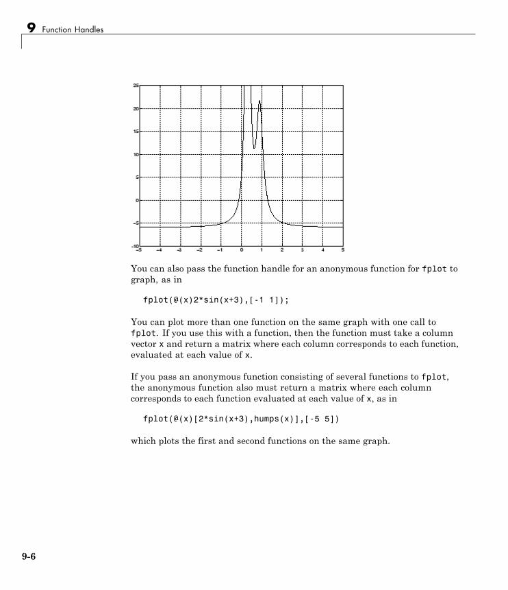
9 Function Handles
You can also pass the function handle for an anonymous function for fplot tograph, as in
fplot(@(x)2*sin(x+3),[-1 1]);
You can plot more than one function on the same graph with one call tofplot. If you use this with a function, then the function must take a columnvector x and return a matrix where each column corresponds to each function,evaluated at each value of x.
If you pass an anonymous function consisting of several functions to fplot,the anonymous function also must return a matrix where each columncorresponds to each function evaluated at each value of x, as in
fplot(@(x)[2*sin(x+3),humps(x)],[-5 5])
which plots the first and second functions on the same graph.
9-6
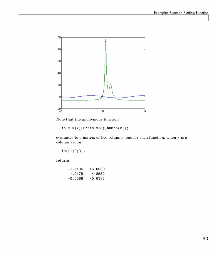
Example: Function Plotting Function
Note that the anonymous function
fh = @(x)[2*sin(x+3),humps(x)];
evaluates to a matrix of two columns, one for each function, when x is acolumn vector.
fh([1;2;3])
returns
-1.5136 16.0000-1.9178 -4.8552-0.5588 -5.6383
9-7
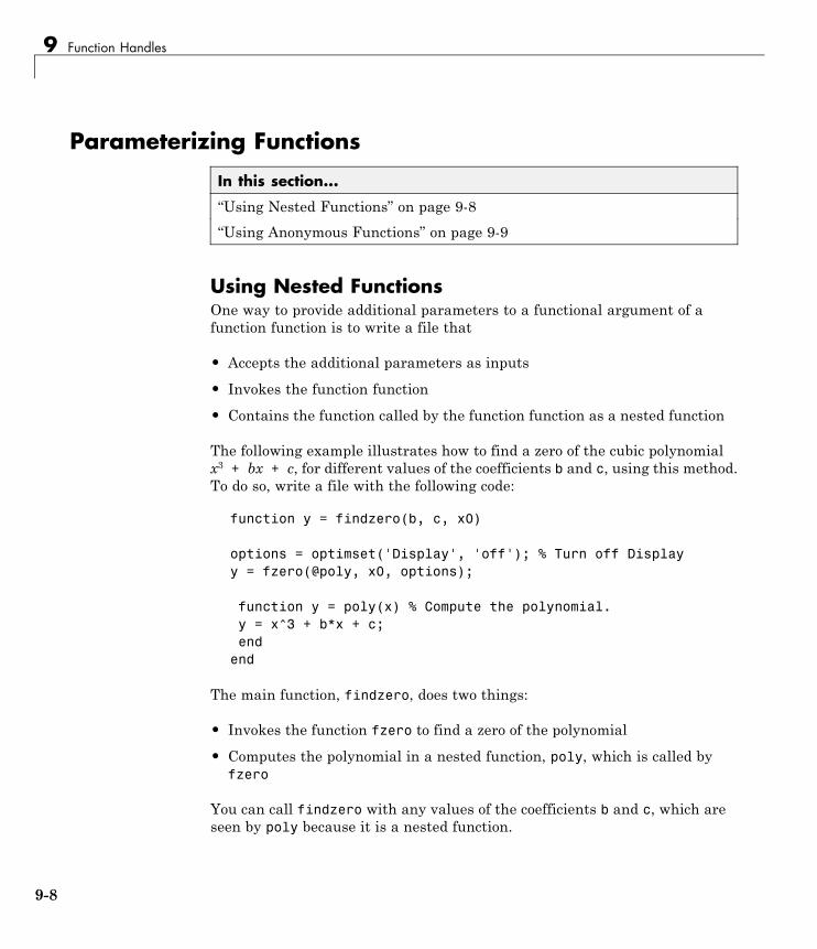
9 Function Handles
Parameterizing Functions
In this section...
“Using Nested Functions” on page 9-8
“Using Anonymous Functions” on page 9-9
Using Nested FunctionsOne way to provide additional parameters to a functional argument of afunction function is to write a file that
• Accepts the additional parameters as inputs
• Invokes the function function
• Contains the function called by the function function as a nested function
The following example illustrates how to find a zero of the cubic polynomialx3 + bx + c, for different values of the coefficients b and c, using this method.To do so, write a file with the following code:
function y = findzero(b, c, x0)
options = optimset('Display', 'off'); % Turn off Displayy = fzero(@poly, x0, options);
function y = poly(x) % Compute the polynomial.y = x^3 + b*x + c;end
end
The main function, findzero, does two things:
• Invokes the function fzero to find a zero of the polynomial
• Computes the polynomial in a nested function, poly, which is called byfzero
You can call findzero with any values of the coefficients b and c, which areseen by poly because it is a nested function.
9-8

Parameterizing Functions
As an example, to find a zero of the polynomial with b = 2 and c = 3.5,using the starting point x0 = 0, call findzero as follows.
x = findzero(2, 3.5, 0)
This returns the zero
x =
-1.0945
Using Anonymous FunctionsSuppose you have already written a standalone file for the function polycontaining the following code, which computes the polynomial for anycoefficients b and c,
function y = poly(x, b, c) % Compute the polynomial.y = x^3 + b*x + c;
You then want to find a zero for the coefficient values b = 2 and c = 3.5.You cannot simply apply fzero to poly, which has three input arguments,because fzero only accepts functions with a single input argument.
As an alternative to rewriting poly as a nested function (see “Using NestedFunctions” on page 9-8) you can pass poly to fzero as a function handle to ananonymous function that has the form @(x) poly(x, b, c). The functionhandle has just one input argument x, so fzero accepts it.
b = 2;c = 3.5;x = fzero(@(x) poly(x, b, c), 0)
This returns the zero
x =
-1.0945
“Anonymous Functions” on page 9-4 explains how to create anonymousfunctions.
9-9
9 Function Handles
If you later decide to find a zero for different values of b and c, you mustredefine the anonymous function using the new values. For example,
b = 4;c = -1;fzero(@(x) poly(x, b, c), 0)
ans =
0.2463
For more complicated objective functions, it is usually preferable to write thefunction as a nested function.
9-10
10
Calculus
• “Ordinary Differential Equations” on page 10-2
• “Delay Differential Equations” on page 10-47
• “Boundary-Value Problems” on page 10-59
• “Partial Differential Equations” on page 10-87
• “Selected Bibliography for Differential Equations” on page 10-105
• “Integration” on page 10-106

10 Calculus
Ordinary Differential Equations
In this section...
“Function Summary” on page 10-2
“Initial Value Problems” on page 10-4
“Types of Solvers” on page 10-6
“Solver Syntax” on page 10-8
“Integrator Options” on page 10-9
“Examples” on page 10-10
“Troubleshooting” on page 10-39
Function Summary
• “ODE Solvers” on page 10-2
• “Evaluation and Extension” on page 10-3
• “Solver Options” on page 10-3
• “Output Functions” on page 10-4
ODE SolversThe following table lists the initial value problem solvers, the kind of problemyou can solve with each solver, and the method each solver uses.
Solver Solves These Kinds ofProblems
Method
ode45 Nonstiff differentialequations
Runge-Kutta
ode23 Nonstiff differentialequations
Runge-Kutta
ode113 Nonstiff differentialequations
Adams
10-2
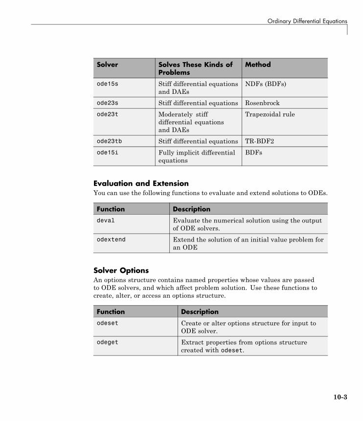
Ordinary Differential Equations
Solver Solves These Kinds ofProblems
Method
ode15s Stiff differential equationsand DAEs
NDFs (BDFs)
ode23s Stiff differential equations Rosenbrock
ode23t Moderately stiffdifferential equationsand DAEs
Trapezoidal rule
ode23tb Stiff differential equations TR-BDF2
ode15i Fully implicit differentialequations
BDFs
Evaluation and ExtensionYou can use the following functions to evaluate and extend solutions to ODEs.
Function Description
deval Evaluate the numerical solution using the outputof ODE solvers.
odextend Extend the solution of an initial value problem foran ODE
Solver OptionsAn options structure contains named properties whose values are passedto ODE solvers, and which affect problem solution. Use these functions tocreate, alter, or access an options structure.
Function Description
odeset Create or alter options structure for input toODE solver.
odeget Extract properties from options structurecreated with odeset.
10-3
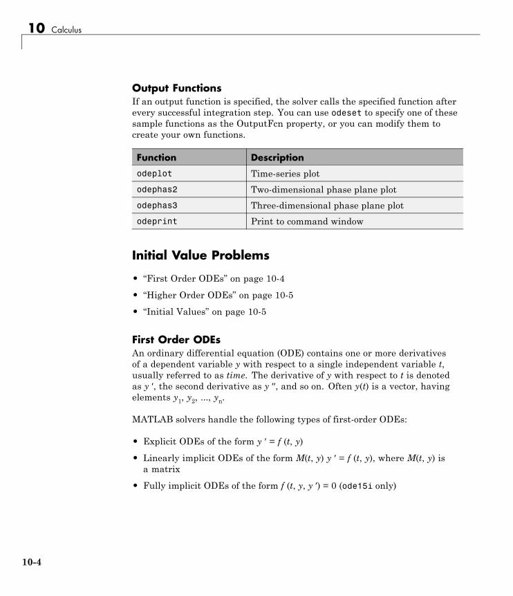
10 Calculus
Output FunctionsIf an output function is specified, the solver calls the specified function afterevery successful integration step. You can use odeset to specify one of thesesample functions as the OutputFcn property, or you can modify them tocreate your own functions.
Function Description
odeplot Time-series plot
odephas2 Two-dimensional phase plane plot
odephas3 Three-dimensional phase plane plot
odeprint Print to command window
Initial Value Problems
• “First Order ODEs” on page 10-4
• “Higher Order ODEs” on page 10-5
• “Initial Values” on page 10-5
First Order ODEsAn ordinary differential equation (ODE) contains one or more derivativesof a dependent variable y with respect to a single independent variable t,usually referred to as time. The derivative of y with respect to t is denotedas y ′, the second derivative as y ′′, and so on. Often y(t) is a vector, havingelements y1, y2, ..., yn.
MATLAB solvers handle the following types of first-order ODEs:
• Explicit ODEs of the form y ′ = f (t, y)
• Linearly implicit ODEs of the form M(t, y) y ′ = f (t, y), where M(t, y) isa matrix
• Fully implicit ODEs of the form f (t, y, y ′) = 0 (ode15i only)
10-4
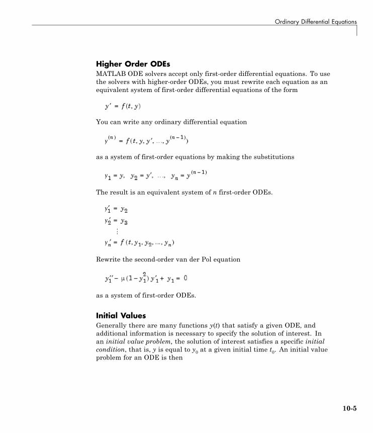
Ordinary Differential Equations
Higher Order ODEsMATLAB ODE solvers accept only first-order differential equations. To usethe solvers with higher-order ODEs, you must rewrite each equation as anequivalent system of first-order differential equations of the form
You can write any ordinary differential equation
as a system of first-order equations by making the substitutions
The result is an equivalent system of n first-order ODEs.
Rewrite the second-order van der Pol equation
as a system of first-order ODEs.
Initial ValuesGenerally there are many functions y(t) that satisfy a given ODE, andadditional information is necessary to specify the solution of interest. Inan initial value problem, the solution of interest satisfies a specific initialcondition, that is, y is equal to y0 at a given initial time t0. An initial valueproblem for an ODE is then
10-5
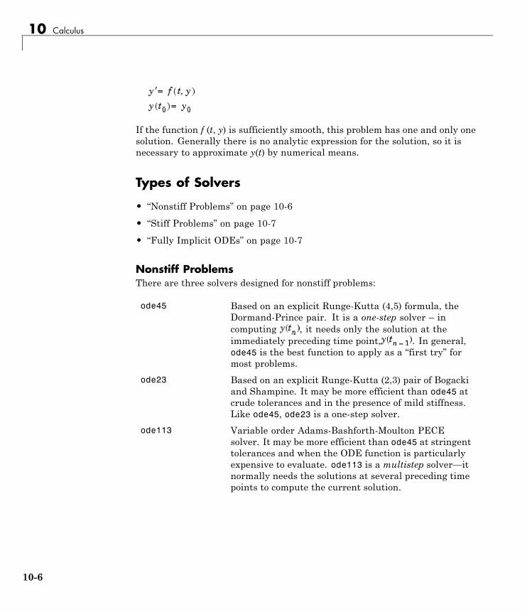
10 Calculus
If the function f (t, y) is sufficiently smooth, this problem has one and only onesolution. Generally there is no analytic expression for the solution, so it isnecessary to approximate y(t) by numerical means.
Types of Solvers
• “Nonstiff Problems” on page 10-6
• “Stiff Problems” on page 10-7
• “Fully Implicit ODEs” on page 10-7
Nonstiff ProblemsThere are three solvers designed for nonstiff problems:
ode45 Based on an explicit Runge-Kutta (4,5) formula, theDormand-Prince pair. It is a one-step solver – incomputing , it needs only the solution at theimmediately preceding time point, . In general,ode45 is the best function to apply as a “first try” formost problems.
ode23 Based on an explicit Runge-Kutta (2,3) pair of Bogackiand Shampine. It may be more efficient than ode45 atcrude tolerances and in the presence of mild stiffness.Like ode45, ode23 is a one-step solver.
ode113 Variable order Adams-Bashforth-Moulton PECEsolver. It may be more efficient than ode45 at stringenttolerances and when the ODE function is particularlyexpensive to evaluate. ode113 is a multistep solver—itnormally needs the solutions at several preceding timepoints to compute the current solution.
10-6
Ordinary Differential Equations
Stiff ProblemsNot all difficult problems are stiff, but all stiff problems are difficult forsolvers not specifically designed for them. Solvers for stiff problems can beused exactly like the other solvers. However, you can often significantlyimprove the efficiency of these solvers by providing them with additionalinformation about the problem. (See “Integrator Options” on page 10-9.)
There are four solvers designed for stiff problems:
ode15s Variable-order solver based on the numericaldifferentiation formulas (NDFs). Optionally it uses thebackward differentiation formulas, BDFs (also knownas Gear’s method). Like ode113, ode15s is a multistepsolver. If you suspect that a problem is stiff or if ode45failed or was very inefficient, try ode15s.
ode23s Based on a modified Rosenbrock formula of order 2.Because it is a one-step solver, it may be more efficientthan ode15s at crude tolerances. It can solve somekinds of stiff problems for which ode15s is not effective.
ode23t An implementation of the trapezoidal rule using a“free” interpolant. Use this solver if the problem isonly moderately stiff and you need a solution withoutnumerical damping.
ode23tb An implementation of TR-BDF2, an implicitRunge-Kutta formula with a first stage that is atrapezoidal rule step and a second stage that is abackward differentiation formula of order 2. Likeode23s, this solver may be more efficient than ode15sat crude tolerances.
Fully Implicit ODEsThe solver ode15i solves fully implicit differential equations of the form
using the variable order BDF method. The basic syntax for ode15i is
10-7

10 Calculus
[t,y] = ode15i(odefun,tspan,y0,yp0,options)
The input arguments are
odefun A function that evaluates the left side of the differentialequation of the form .
tspan A vector specifying the interval of integration, [t0,tf].To obtain solutions at specific times (all increasing or alldecreasing), use tspan = [t0,t1,...,tf].
y0, yp0 Vectors of initial conditions for and , respectively.The specified values must be consistent; that is, they mustsatisfy f(t0,y0,yp0) = 0.
options Optional integration argument created using the odesetfunction. See the odeset reference page for details.
The output arguments contain the solution approximated at discrete points:
t Column vector of time points
y Solution array. Each row in y corresponds to the solution ata time returned in the corresponding row of t.
See the ode15i reference page for more information about these arguments.
Solver SyntaxAll of the ODE solver functions, except for ode15i, share a syntax that makesit easy to try any of the different numerical methods, if it is not apparentwhich is the most appropriate. To apply a different method to the sameproblem, simply change the ODE solver function name. The simplest syntax,common to all the solver functions, is
[t,y] = solver(odefun,tspan,y0,options)
where solver is one of the ODE solver functions listed previously.
The basic input arguments are
10-8
Ordinary Differential Equations
odefun Handle to a function that evaluates the system ofODEs. The function has the form
dydt = odefun(t,y)
where t is a scalar, and dydt and y are column vectors.See “Function Handles” in MATLAB ProgrammingFundamentals for more information.
tspan Vector specifying the interval of integration. Thesolver imposes the initial conditions at tspan(1), andintegrates from tspan(1) to tspan(end).
y0 Vector of initial conditions for the problem
See also “Initial Value Problems” on page 10-4.
options Structure of optional parameters that change thedefault integration properties.
“Integrator Options” on page 10-9 tells you how tocreate the structure and describes the properties youcan specify.
The output arguments contain the solution approximated at discrete points:
t Column vector of time points
y Solution array. Each row in y corresponds to thesolution at a time returned in the corresponding rowof t.
See the reference page for the ODE solvers for more information about thesearguments.
Integrator OptionsThe default integration properties in the ODE solvers are selected to handlecommon problems. In some cases, you can improve ODE solver performanceby overriding these defaults. You do this by supplying the solvers with anoptions structure that specifies one or more property values.
10-9
10 Calculus
For example, to change the value of the relative error tolerance of the solverfrom the default value of 1e-3 to 1e-4,
1 Create an options structure using the function odeset by entering
options = odeset('RelTol', 1e-4);
2 Pass the options structure to the solver as follows:
• For all solvers except ode15i, use the syntax
[t,y] = solver(odefun,tspan,y0,options)
• For ode15i, use the syntax
[t,y] = ode15i(odefun,tspan,y0,yp0,options)
For a complete description of the available options, see the reference pagefor odeset.
Examples
• “van der Pol Equation (Nonstiff)” on page 10-11
• “van der Pol Equation (Stiff)” on page 10-13
• “van der Pol Equation (Parameterizing the ODE)” on page 10-15
• “van der Pol Equation (Evaluating the Solution)” on page 10-16
• “Euler Equations (Nonstiff)” on page 10-16
• “Fully Implicit ODE” on page 10-18
• “Finite Element Discretization” on page 10-19
• “Large Stiff Sparse Problem” on page 10-22
• “Event Location” on page 10-25
• “Advanced Event Location” on page 10-28
• “Differential-Algebraic Equations” on page 10-31
• “Nonnegative Solutions” on page 10-34
10-10
Ordinary Differential Equations
• “Additional Examples” on page 10-38
van der Pol Equation (Nonstiff)This example illustrates the steps for solving an initial value ODE problem:
1 Rewrite the problem as a system of first-order ODEs. Rewrite thevan der Pol equation (second-order)
where is a scalar parameter, by making the substitution .The resulting system of first-order ODEs is
2 Code the system of first-order ODEs. Once you represent the equationas a system of first-order ODEs, you can code it as a function that an ODEsolver can use. The function must be of the form
dydt = odefun(t,y)
Although t and y must be the function’s two arguments, the function doesnot need to use them. The output dydt, a column vector, is the derivativeof y.
The code below represents the van der Pol system in the function, vdp1.The vdp1 function assumes that . The variables and are theentries y(1) and y(2) of a two-element vector.
function dydt = vdp1(t,y)dydt = [y(2); (1-y(1)^2)*y(2)-y(1)];
Note that, although vdp1 must accept the arguments t and y, it does notuse t in its computations.
3 Apply a solver to the problem.
10-11
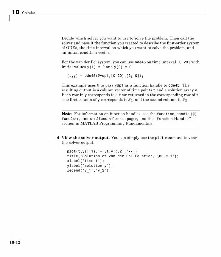
10 Calculus
Decide which solver you want to use to solve the problem. Then call thesolver and pass it the function you created to describe the first-order systemof ODEs, the time interval on which you want to solve the problem, andan initial condition vector.
For the van der Pol system, you can use ode45 on time interval [0 20] withinitial values y(1) = 2 and y(2) = 0.
[t,y] = ode45(@vdp1,[0 20],[2; 0]);
This example uses @ to pass vdp1 as a function handle to ode45. Theresulting output is a column vector of time points t and a solution array y.Each row in y corresponds to a time returned in the corresponding row of t.The first column of y corresponds to , and the second column to .
Note For information on function handles, see the function_handle (@),func2str, and str2func reference pages, and the “Function Handles”section in MATLAB Programming Fundamentals.
4 View the solver output. You can simply use the plot command to viewthe solver output.
plot(t,y(:,1),'-',t,y(:,2),'--')title('Solution of van der Pol Equation, \mu = 1');xlabel('time t');ylabel('solution y');legend('y_1','y_2')
10-12
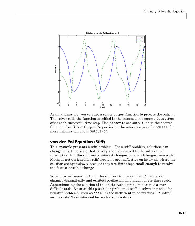
Ordinary Differential Equations
As an alternative, you can use a solver output function to process the output.The solver calls the function specified in the integration property OutputFcnafter each successful time step. Use odeset to set OutputFcn to the desiredfunction. See Solver Output Properties, in the reference page for odeset, formore information about OutputFcn.
van der Pol Equation (Stiff)This example presents a stiff problem. For a stiff problem, solutions canchange on a time scale that is very short compared to the interval ofintegration, but the solution of interest changes on a much longer time scale.Methods not designed for stiff problems are ineffective on intervals where thesolution changes slowly because they use time steps small enough to resolvethe fastest possible change.
When is increased to 1000, the solution to the van der Pol equationchanges dramatically and exhibits oscillation on a much longer time scale.Approximating the solution of the initial value problem becomes a moredifficult task. Because this particular problem is stiff, a solver intended fornonstiff problems, such as ode45, is too inefficient to be practical. A solversuch as ode15s is intended for such stiff problems.
10-13

10 Calculus
The vdp1000 function evaluates the van der Pol system from the previousexample, but with = 1000.
function dydt = vdp1000(t,y)dydt = [y(2); 1000*(1-y(1)^2)*y(2)-y(1)];
Note This example hardcodes in the ODE function. The vdpode examplesolves the same problem, but passes a user-specified as a parameter tothe ODE function.
Now use the ode15s function to solve the problem with the initial conditionvector of [2; 0], but a time interval of [0 3000]. For scaling reasons, plotjust the first component of y(t).
[t,y] = ode15s(@vdp1000,[0 3000],[2; 0]);plot(t,y(:,1),'-');title('Solution of van der Pol Equation, \mu = 1000');xlabel('time t');ylabel('solution y_1');
10-14
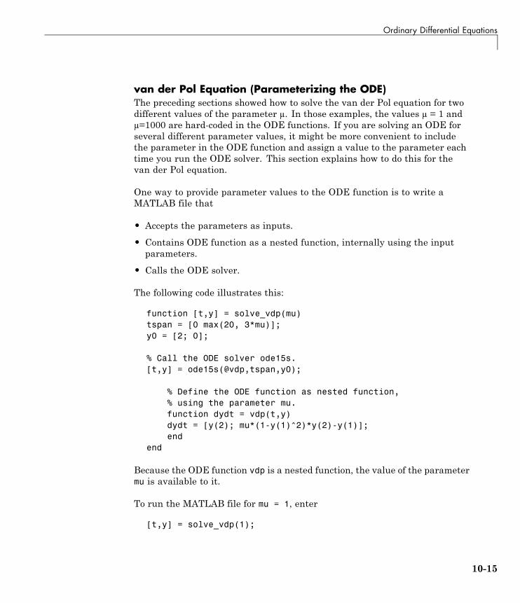
Ordinary Differential Equations
van der Pol Equation (Parameterizing the ODE)The preceding sections showed how to solve the van der Pol equation for twodifferent values of the parameter µ. In those examples, the values µ = 1 andµ=1000 are hard-coded in the ODE functions. If you are solving an ODE forseveral different parameter values, it might be more convenient to includethe parameter in the ODE function and assign a value to the parameter eachtime you run the ODE solver. This section explains how to do this for thevan der Pol equation.
One way to provide parameter values to the ODE function is to write aMATLAB file that
• Accepts the parameters as inputs.
• Contains ODE function as a nested function, internally using the inputparameters.
• Calls the ODE solver.
The following code illustrates this:
function [t,y] = solve_vdp(mu)tspan = [0 max(20, 3*mu)];y0 = [2; 0];
% Call the ODE solver ode15s.[t,y] = ode15s(@vdp,tspan,y0);
% Define the ODE function as nested function,% using the parameter mu.function dydt = vdp(t,y)dydt = [y(2); mu*(1-y(1)^2)*y(2)-y(1)];end
end
Because the ODE function vdp is a nested function, the value of the parametermu is available to it.
To run the MATLAB file for mu = 1, enter
[t,y] = solve_vdp(1);
10-15

10 Calculus
To run the code for µ = 1000, enter
[t,y] = solve_vdp(1000);
See the vdpode code for a complete example based on these functions.
van der Pol Equation (Evaluating the Solution)The numerical methods implemented in the ODE solvers produce acontinuous solution over the interval of integration . You can evaluatethe approximate solution, , at any point in using the function devaland the structure sol returned by the solver. For example, if you solve theproblem described in “van der Pol Equation (Nonstiff)” on page 10-11 bycalling ode45 with a single output argument sol,
sol = ode45(@vdp1,[0 20],[2; 0]);
ode45 returns the solution as a structure. You can then evaluate theapproximate solution at points in the vector xint = 1:5 as follows:
xint = 1:5;Sxint = deval(sol,xint)
Sxint =
1.5081 0.3235 -1.8686 -1.7407 -0.8344-0.7803 -1.8320 -1.0220 0.6260 1.3095
The deval function is vectorized. For a vector xint, the ith column of Sxintapproximates the solution .
Euler Equations (Nonstiff)rigidode illustrates the solution of a standard test problem proposed byKrogh for solvers intended for nonstiff problems [8].
The ODEs are the Euler equations of a rigid body without external forces.
10-16
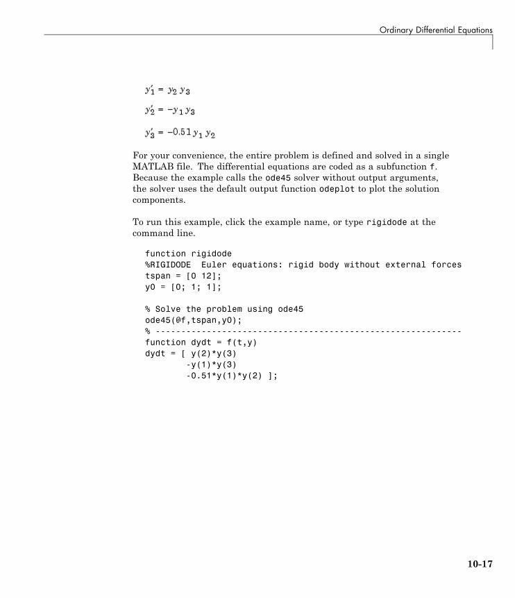
Ordinary Differential Equations
For your convenience, the entire problem is defined and solved in a singleMATLAB file. The differential equations are coded as a subfunction f.Because the example calls the ode45 solver without output arguments,the solver uses the default output function odeplot to plot the solutioncomponents.
To run this example, click the example name, or type rigidode at thecommand line.
function rigidode%RIGIDODE Euler equations: rigid body without external forcestspan = [0 12];y0 = [0; 1; 1];
% Solve the problem using ode45ode45(@f,tspan,y0);% ------------------------------------------------------------function dydt = f(t,y)dydt = [ y(2)*y(3)
-y(1)*y(3)-0.51*y(1)*y(2) ];
10-17
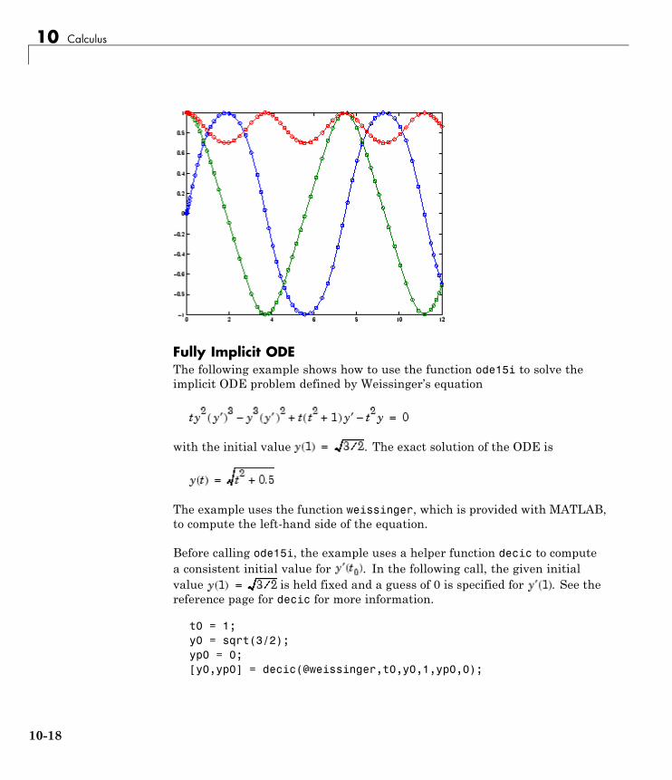
10 Calculus
Fully Implicit ODEThe following example shows how to use the function ode15i to solve theimplicit ODE problem defined by Weissinger’s equation
with the initial value . The exact solution of the ODE is
The example uses the function weissinger, which is provided with MATLAB,to compute the left-hand side of the equation.
Before calling ode15i, the example uses a helper function decic to computea consistent initial value for . In the following call, the given initialvalue is held fixed and a guess of 0 is specified for . See thereference page for decic for more information.
t0 = 1;y0 = sqrt(3/2);yp0 = 0;[y0,yp0] = decic(@weissinger,t0,y0,1,yp0,0);
10-18
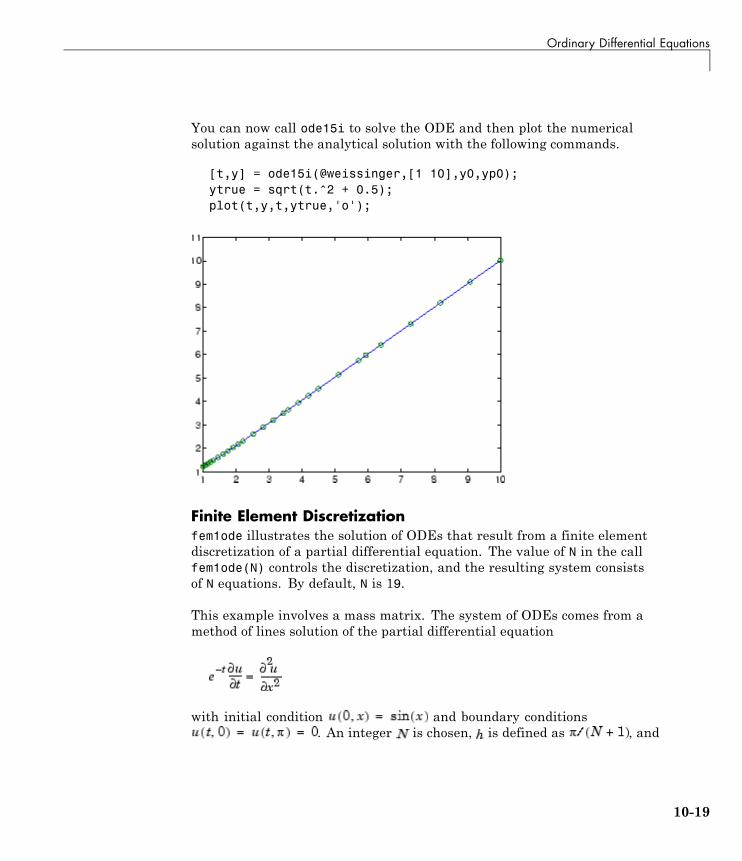
Ordinary Differential Equations
You can now call ode15i to solve the ODE and then plot the numericalsolution against the analytical solution with the following commands.
[t,y] = ode15i(@weissinger,[1 10],y0,yp0);ytrue = sqrt(t.^2 + 0.5);plot(t,y,t,ytrue,'o');
Finite Element Discretizationfem1ode illustrates the solution of ODEs that result from a finite elementdiscretization of a partial differential equation. The value of N in the callfem1ode(N) controls the discretization, and the resulting system consistsof N equations. By default, N is 19.
This example involves a mass matrix. The system of ODEs comes from amethod of lines solution of the partial differential equation
with initial condition and boundary conditions. An integer is chosen, is defined as , and
10-19
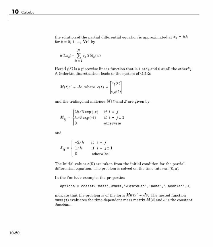
10 Calculus
the solution of the partial differential equation is approximated atfor k = 0, 1, ..., N+1 by
Here is a piecewise linear function that is 1 at and 0 at all the other .A Galerkin discretization leads to the system of ODEs
and the tridiagonal matrices and are given by
and
The initial values are taken from the initial condition for the partialdifferential equation. The problem is solved on the time interval .
In the fem1ode example, the properties
options = odeset('Mass',@mass,'MStateDep','none','Jacobian',J)
indicate that the problem is of the form . The nested functionmass(t) evaluates the time-dependent mass matrix and J is the constantJacobian.
10-20
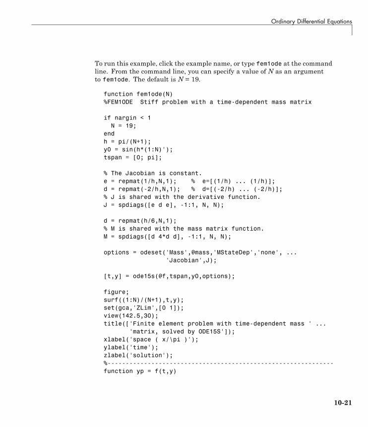
Ordinary Differential Equations
To run this example, click the example name, or type fem1ode at the commandline. From the command line, you can specify a value of N as an argumentto fem1ode. The default is N = 19.
function fem1ode(N)%FEM1ODE Stiff problem with a time-dependent mass matrix
if nargin < 1N = 19;
endh = pi/(N+1);y0 = sin(h*(1:N)');tspan = [0; pi];
% The Jacobian is constant.e = repmat(1/h,N,1); % e=[(1/h) ... (1/h)];d = repmat(-2/h,N,1); % d=[(-2/h) ... (-2/h)];% J is shared with the derivative function.J = spdiags([e d e], -1:1, N, N);
d = repmat(h/6,N,1);% M is shared with the mass matrix function.M = spdiags([d 4*d d], -1:1, N, N);
options = odeset('Mass',@mass,'MStateDep','none', ...'Jacobian',J);
[t,y] = ode15s(@f,tspan,y0,options);
figure;surf((1:N)/(N+1),t,y);set(gca,'ZLim',[0 1]);view(142.5,30);title(['Finite element problem with time-dependent mass ' ...
'matrix, solved by ODE15S']);xlabel('space ( x/\pi )');ylabel('time');zlabel('solution');%--------------------------------------------------------------function yp = f(t,y)
10-21
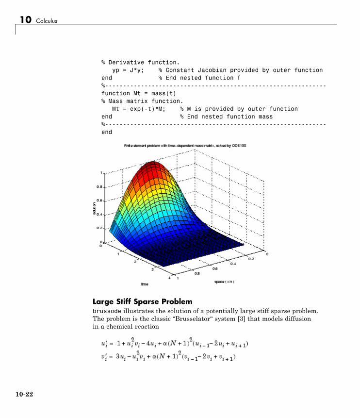
10 Calculus
% Derivative function.yp = J*y; % Constant Jacobian provided by outer function
end % End nested function f%--------------------------------------------------------------function Mt = mass(t)% Mass matrix function.
Mt = exp(-t)*M; % M is provided by outer functionend % End nested function mass%--------------------------------------------------------------end
Large Stiff Sparse Problembrussode illustrates the solution of a potentially large stiff sparse problem.The problem is the classic “Brusselator“ system [3] that models diffusionin a chemical reaction
10-22
Ordinary Differential Equations
and is solved on the time interval [0,10] with = 1/50 and
There are equations in the system, but the Jacobian is banded with aconstant width 5 if the equations are ordered as
In the call brussode(N), where N corresponds to , the parameter N ≥ 2specifies the number of grid points. The resulting system consists of 2Nequations. By default, N is 20. The problem becomes increasingly stiff andthe Jacobian increasingly sparse as N increases.
The nested function f(t,y) returns the derivatives vector for the Brusselatorproblem. The subfunction jpattern(N) returns a sparse matrix of 1s and 0sshowing the locations of nonzeros in the Jacobian . The example assignsthis matrix to the property JPattern, and the solver uses the sparsity patternto generate the Jacobian numerically as a sparse matrix. Providing a sparsitypattern can significantly reduce the number of function evaluations requiredto generate the Jacobian and can accelerate integration.
For the Brusselator problem, if the sparsity pattern is not supplied, 2Nevaluations of the function are needed to compute the 2N-by-2N Jacobianmatrix. If the sparsity pattern is supplied, only four evaluations are needed,regardless of the value of N.
To run this example, click on the example name, or type brussode at thecommand line. From the command line, you can specify a value of as anargument to brussode. The default is = 20.
function brussode(N)%BRUSSODE Stiff problem modeling a chemical reaction
if nargin < 1N = 20;
end
tspan = [0; 10];y0 = [1+sin((2*pi/(N+1))*(1:N));repmat(3,1,N)];
10-23
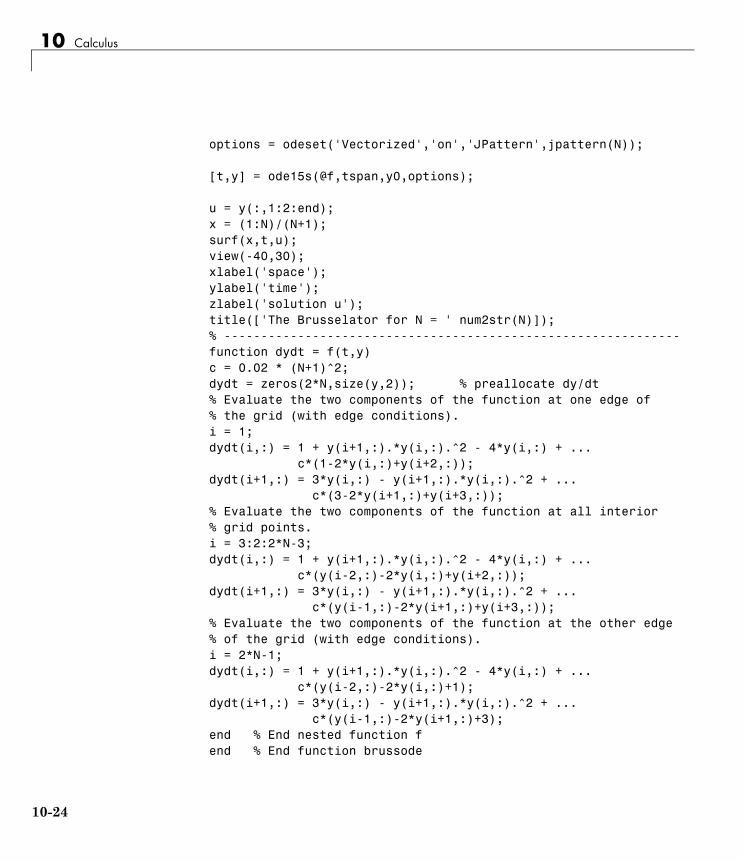
10 Calculus
options = odeset('Vectorized','on','JPattern',jpattern(N));
[t,y] = ode15s(@f,tspan,y0,options);
u = y(:,1:2:end);x = (1:N)/(N+1);surf(x,t,u);view(-40,30);xlabel('space');ylabel('time');zlabel('solution u');title(['The Brusselator for N = ' num2str(N)]);% --------------------------------------------------------------function dydt = f(t,y)c = 0.02 * (N+1)^2;dydt = zeros(2*N,size(y,2)); % preallocate dy/dt% Evaluate the two components of the function at one edge of% the grid (with edge conditions).i = 1;dydt(i,:) = 1 + y(i+1,:).*y(i,:).^2 - 4*y(i,:) + ...
c*(1-2*y(i,:)+y(i+2,:));dydt(i+1,:) = 3*y(i,:) - y(i+1,:).*y(i,:).^2 + ...
c*(3-2*y(i+1,:)+y(i+3,:));% Evaluate the two components of the function at all interior% grid points.i = 3:2:2*N-3;dydt(i,:) = 1 + y(i+1,:).*y(i,:).^2 - 4*y(i,:) + ...
c*(y(i-2,:)-2*y(i,:)+y(i+2,:));dydt(i+1,:) = 3*y(i,:) - y(i+1,:).*y(i,:).^2 + ...
c*(y(i-1,:)-2*y(i+1,:)+y(i+3,:));% Evaluate the two components of the function at the other edge% of the grid (with edge conditions).i = 2*N-1;dydt(i,:) = 1 + y(i+1,:).*y(i,:).^2 - 4*y(i,:) + ...
c*(y(i-2,:)-2*y(i,:)+1);dydt(i+1,:) = 3*y(i,:) - y(i+1,:).*y(i,:).^2 + ...
c*(y(i-1,:)-2*y(i+1,:)+3);end % End nested function fend % End function brussode
10-24
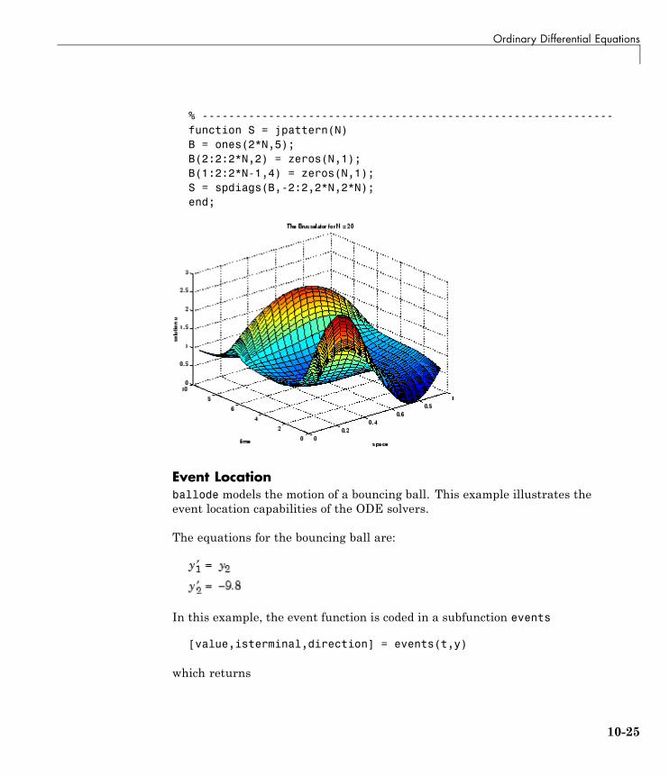
Ordinary Differential Equations
% --------------------------------------------------------------function S = jpattern(N)B = ones(2*N,5);B(2:2:2*N,2) = zeros(N,1);B(1:2:2*N-1,4) = zeros(N,1);S = spdiags(B,-2:2,2*N,2*N);end;
Event Locationballode models the motion of a bouncing ball. This example illustrates theevent location capabilities of the ODE solvers.
The equations for the bouncing ball are:
In this example, the event function is coded in a subfunction events
[value,isterminal,direction] = events(t,y)
which returns
10-25
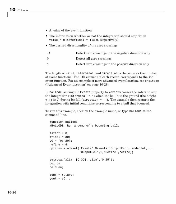
10 Calculus
• A value of the event function
• The information whether or not the integration should stop whenvalue = 0 (isterminal = 1 or 0, respectively)
• The desired directionality of the zero crossings:
-1 Detect zero crossings in the negative direction only
0 Detect all zero crossings
1 Detect zero crossings in the positive direction only
The length of value, isterminal, and direction is the same as the numberof event functions. The ith element of each vector, corresponds to the ithevent function. For an example of more advanced event location, see orbitode(“Advanced Event Location” on page 10-28).
In ballode, setting the Events property to @events causes the solver to stopthe integration (isterminal = 1) when the ball hits the ground (the heighty(1) is 0) during its fall (direction = -1). The example then restarts theintegration with initial conditions corresponding to a ball that bounced.
To run this example, click on the example name, or type ballode at thecommand line.
function ballode%BALLODE Run a demo of a bouncing ball.
tstart = 0;tfinal = 30;y0 = [0; 20];refine = 4;options = odeset('Events',@events,'OutputFcn', @odeplot,...
'OutputSel',1,'Refine',refine);
set(gca,'xlim',[0 30],'ylim',[0 25]);box onhold on;
tout = tstart;yout = y0.';
10-26
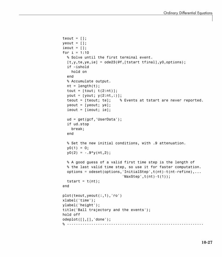
Ordinary Differential Equations
teout = [];yeout = [];ieout = [];for i = 1:10
% Solve until the first terminal event.[t,y,te,ye,ie] = ode23(@f,[tstart tfinal],y0,options);if ~ishold
hold onend% Accumulate output.nt = length(t);tout = [tout; t(2:nt)];yout = [yout; y(2:nt,:)];teout = [teout; te]; % Events at tstart are never reported.yeout = [yeout; ye];ieout = [ieout; ie];
ud = get(gcf,'UserData');if ud.stop
break;end
% Set the new initial conditions, with .9 attenuation.y0(1) = 0;y0(2) = -.9*y(nt,2);
% A good guess of a valid first time step is the length of% the last valid time step, so use it for faster computation.options = odeset(options,'InitialStep',t(nt)-t(nt-refine),...
'MaxStep',t(nt)-t(1));tstart = t(nt);
end
plot(teout,yeout(:,1),'ro')xlabel('time');ylabel('height');title('Ball trajectory and the events');hold offodeplot([],[],'done');% --------------------------------------------------------------
10-27
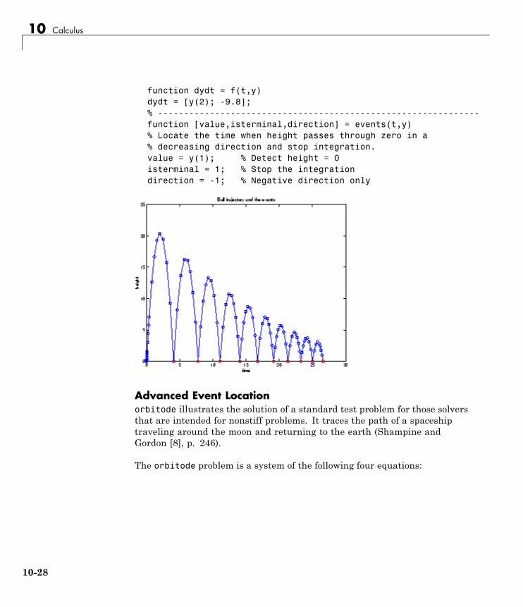
10 Calculus
function dydt = f(t,y)dydt = [y(2); -9.8];% --------------------------------------------------------------function [value,isterminal,direction] = events(t,y)% Locate the time when height passes through zero in a% decreasing direction and stop integration.value = y(1); % Detect height = 0isterminal = 1; % Stop the integrationdirection = -1; % Negative direction only
Advanced Event Locationorbitode illustrates the solution of a standard test problem for those solversthat are intended for nonstiff problems. It traces the path of a spaceshiptraveling around the moon and returning to the earth (Shampine andGordon [8], p. 246).
The orbitode problem is a system of the following four equations:
10-28

Ordinary Differential Equations
where
The first two solution components are coordinates of the body of infinitesimalmass, so plotting one against the other gives the orbit of the body. Theinitial conditions have been chosen to make the orbit periodic. The valueof corresponds to a spaceship traveling around the moon and the earth.Moderately stringent tolerances are necessary to reproduce the qualitativebehavior of the orbit. Suitable values are 1e-5 for RelTol and 1e-4 for AbsTol.
The nested events function includes event functions that locate the point ofmaximum distance from the starting point and the time the spaceship returnsto the starting point. Note that the events are located accurately, even thoughthe step sizes used by the integrator are not determined by the location ofthe events. In this example, the ability to specify the direction of the zerocrossing is critical. Both the point of return to the initial point and the pointof maximum distance have the same event function value, and the direction ofthe crossing is used to distinguish them.
To run this example, click on the example name, or type orbitode at thecommand line. The example uses the output function odephas2 to produce
10-29
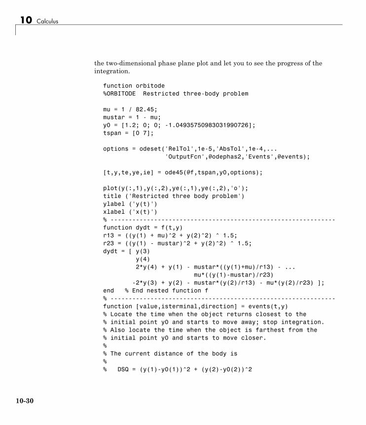
10 Calculus
the two-dimensional phase plane plot and let you to see the progress of theintegration.
function orbitode%ORBITODE Restricted three-body problem
mu = 1 / 82.45;mustar = 1 - mu;y0 = [1.2; 0; 0; -1.04935750983031990726];tspan = [0 7];
options = odeset('RelTol',1e-5,'AbsTol',1e-4,...'OutputFcn',@odephas2,'Events',@events);
[t,y,te,ye,ie] = ode45(@f,tspan,y0,options);
plot(y(:,1),y(:,2),ye(:,1),ye(:,2),'o');title ('Restricted three body problem')ylabel ('y(t)')xlabel ('x(t)')% --------------------------------------------------------------function dydt = f(t,y)r13 = ((y(1) + mu)^2 + y(2)^2) ^ 1.5;r23 = ((y(1) - mustar)^2 + y(2)^2) ^ 1.5;dydt = [ y(3)
y(4)2*y(4) + y(1) - mustar*((y(1)+mu)/r13) - ...
mu*((y(1)-mustar)/r23)-2*y(3) + y(2) - mustar*(y(2)/r13) - mu*(y(2)/r23) ];
end % End nested function f% --------------------------------------------------------------function [value,isterminal,direction] = events(t,y)% Locate the time when the object returns closest to the% initial point y0 and starts to move away; stop integration.% Also locate the time when the object is farthest from the% initial point y0 and starts to move closer.%% The current distance of the body is%% DSQ = (y(1)-y0(1))^2 + (y(2)-y0(2))^2
10-30
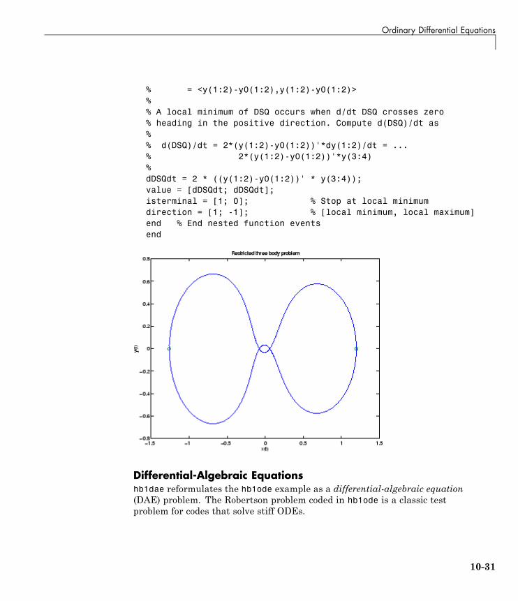
Ordinary Differential Equations
% = <y(1:2)-y0(1:2),y(1:2)-y0(1:2)>%% A local minimum of DSQ occurs when d/dt DSQ crosses zero% heading in the positive direction. Compute d(DSQ)/dt as%% d(DSQ)/dt = 2*(y(1:2)-y0(1:2))'*dy(1:2)/dt = ...% 2*(y(1:2)-y0(1:2))'*y(3:4)%dDSQdt = 2 * ((y(1:2)-y0(1:2))' * y(3:4));value = [dDSQdt; dDSQdt];isterminal = [1; 0]; % Stop at local minimumdirection = [1; -1]; % [local minimum, local maximum]end % End nested function eventsend
Differential-Algebraic Equationshb1dae reformulates the hb1ode example as a differential-algebraic equation(DAE) problem. The Robertson problem coded in hb1ode is a classic testproblem for codes that solve stiff ODEs.
10-31
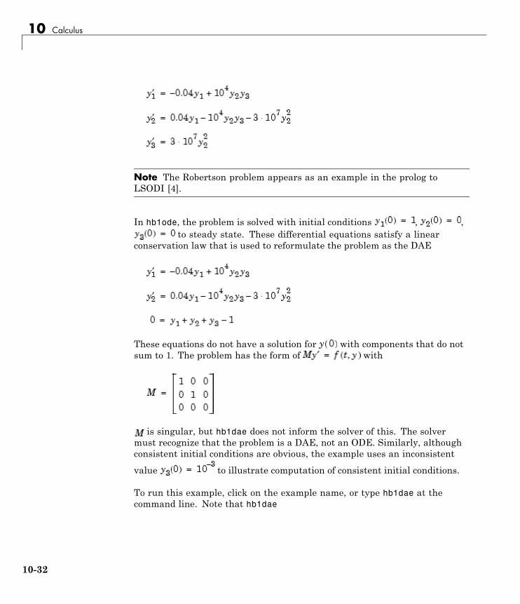
10 Calculus
Note The Robertson problem appears as an example in the prolog toLSODI [4].
In hb1ode, the problem is solved with initial conditions , ,to steady state. These differential equations satisfy a linear
conservation law that is used to reformulate the problem as the DAE
These equations do not have a solution for with components that do notsum to 1. The problem has the form of with
is singular, but hb1dae does not inform the solver of this. The solvermust recognize that the problem is a DAE, not an ODE. Similarly, althoughconsistent initial conditions are obvious, the example uses an inconsistent
value to illustrate computation of consistent initial conditions.
To run this example, click on the example name, or type hb1dae at thecommand line. Note that hb1dae
10-32
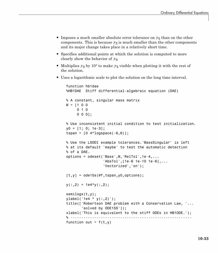
Ordinary Differential Equations
• Imposes a much smaller absolute error tolerance on than on the othercomponents. This is because is much smaller than the other componentsand its major change takes place in a relatively short time.
• Specifies additional points at which the solution is computed to moreclearly show the behavior of .
• Multiplies by 104 to make visible when plotting it with the rest ofthe solution.
• Uses a logarithmic scale to plot the solution on the long time interval.
function hb1dae%HB1DAE Stiff differential-algebraic equation (DAE)
% A constant, singular mass matrixM = [1 0 0
0 1 00 0 0];
% Use inconsistent initial condition to test initialization.y0 = [1; 0; 1e-3];tspan = [0 4*logspace(-6,6)];
% Use the LSODI example tolerances.'MassSingular' is left% at its default 'maybe' to test the automatic detection% of a DAE.options = odeset('Mass',M,'RelTol',1e-4,...
'AbsTol',[1e-6 1e-10 1e-6],...'Vectorized','on');
[t,y] = ode15s(@f,tspan,y0,options);
y(:,2) = 1e4*y(:,2);
semilogx(t,y);ylabel('1e4 * y(:,2)');title(['Robertson DAE problem with a Conservation Law, '...
'solved by ODE15S']);xlabel('This is equivalent to the stiff ODEs in HB1ODE.');% --------------------------------------------------------function out = f(t,y)
10-33
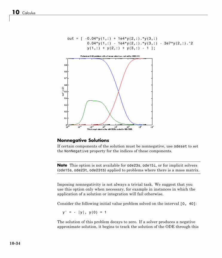
10 Calculus
out = [ -0.04*y(1,:) + 1e4*y(2,:).*y(3,:)0.04*y(1,:) - 1e4*y(2,:).*y(3,:) - 3e7*y(2,:).^2y(1,:) + y(2,:) + y(3,:) - 1 ];
Nonnegative SolutionsIf certain components of the solution must be nonnegative, use odeset to setthe NonNegative property for the indices of these components.
Note This option is not available for ode23s, ode15i, or for implicit solvers(ode15s, ode23t, ode23tb) applied to problems where there is a mass matrix.
Imposing nonnegativity is not always a trivial task. We suggest that youuse this option only when necessary, for example in instances in which theapplication of a solution or integration will fail otherwise.
Consider the following initial value problem solved on the interval [0, 40]:
y' = - |y|, y(0) = 1
The solution of this problem decays to zero. If a solver produces a negativeapproximate solution, it begins to track the solution of the ODE through this
10-34
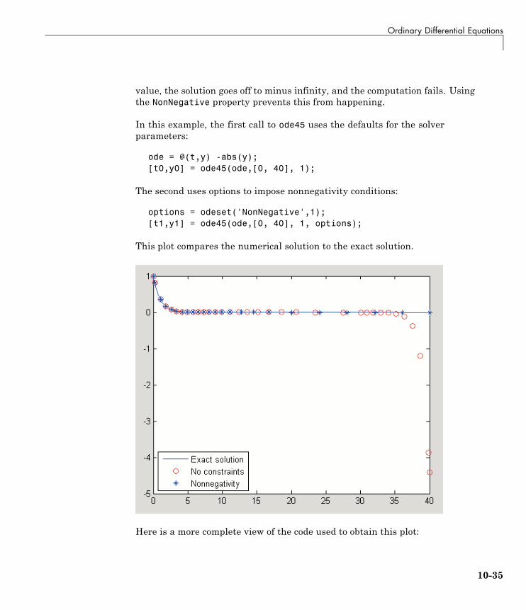
Ordinary Differential Equations
value, the solution goes off to minus infinity, and the computation fails. Usingthe NonNegative property prevents this from happening.
In this example, the first call to ode45 uses the defaults for the solverparameters:
ode = @(t,y) -abs(y);[t0,y0] = ode45(ode,[0, 40], 1);
The second uses options to impose nonnegativity conditions:
options = odeset('NonNegative',1);[t1,y1] = ode45(ode,[0, 40], 1, options);
This plot compares the numerical solution to the exact solution.
Here is a more complete view of the code used to obtain this plot:
10-35
10 Calculus
ode = @(t,y) -abs(y);options = odeset('Refine',1);[t0,y0] = ode45(ode,[0, 40], 1,options);options = odeset(options,'NonNegative',1);[t1,y1] = ode45(ode,[0, 40], 1, options);t = linspace(0,40,1000);y = exp(-t);plot(t,y,'b-',t0,y0,'ro',t1,y1,'b*');legend('Exact solution','No constraints','Nonnegativity', ...
'Location','SouthWest')
The kneeode Demo. The MATLAB kneeode demo solves the “kneeproblem” by imposing a nonnegativity constraint on the numerical solution.The initial value problem is
*y' = (1-x)*y - y^2, y(0) = 1
For 0 < ε < 1, the solution of this problem approaches null isoclines y = 1- x and y = 0 for x < 1 and x > 1, respectively. The numerical solution,when computed with default tolerances, follows the y = 1 - x isocline for thewhole interval of integration. Imposing nonnegativity constraints results inthe correct solution.
Here is the code that makes up the kneeode demo:
function kneeode%KNEEODE The "knee problem" with Nonnegativity constraints.
% Problem parameterepsilon = 1e-6;
y0 = 1;xspan = [0, 2];
% Solve without imposing constraintsoptions = [];[x1,y1] = ode15s(@odefcn,xspan,y0,options);
% Impose nonnegativity constraintoptions = odeset('NonNegative',1);
10-36
Ordinary Differential Equations
[x2,y2] = ode15s(@odefcn,xspan,y0,options);
figureplot(x1,y1,'b.-',x2,y2,'g-')axis([0,2,-1,1]);title('The "knee problem"');legend('No constraints','nonnegativity')xlabel('x');ylabel('solution y')
function yp = odefcn(x,y)yp = ((1 - x)*y - y^2)/epsilon;
endend % kneeode
The derivative function is defined within nested function odefcn. The valueof epsilon used in odefcn is obtained from the outer function:
function yp = odefcn(x,y)yp = ((1 - x)*y - y^2)/epsilon;end
The demo solves the problem using the ode15s function, first with the defaultoptions, and then by imposing a nonnegativity constraint. To run the demo,type kneeode at the MATLAB command prompt.
Here is the output plot. The plot confirms correct solution behavior afterimposing constraints.
10-37
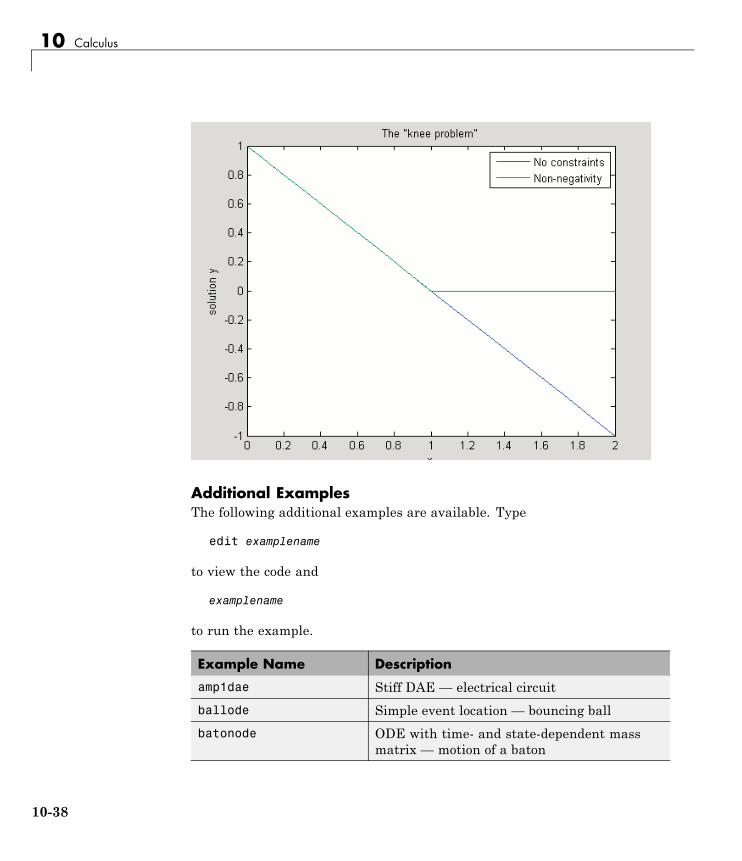
10 Calculus
Additional ExamplesThe following additional examples are available. Type
edit examplename
to view the code and
examplename
to run the example.
Example Name Description
amp1dae Stiff DAE — electrical circuit
ballode Simple event location — bouncing ball
batonode ODE with time- and state-dependent massmatrix — motion of a baton
10-38
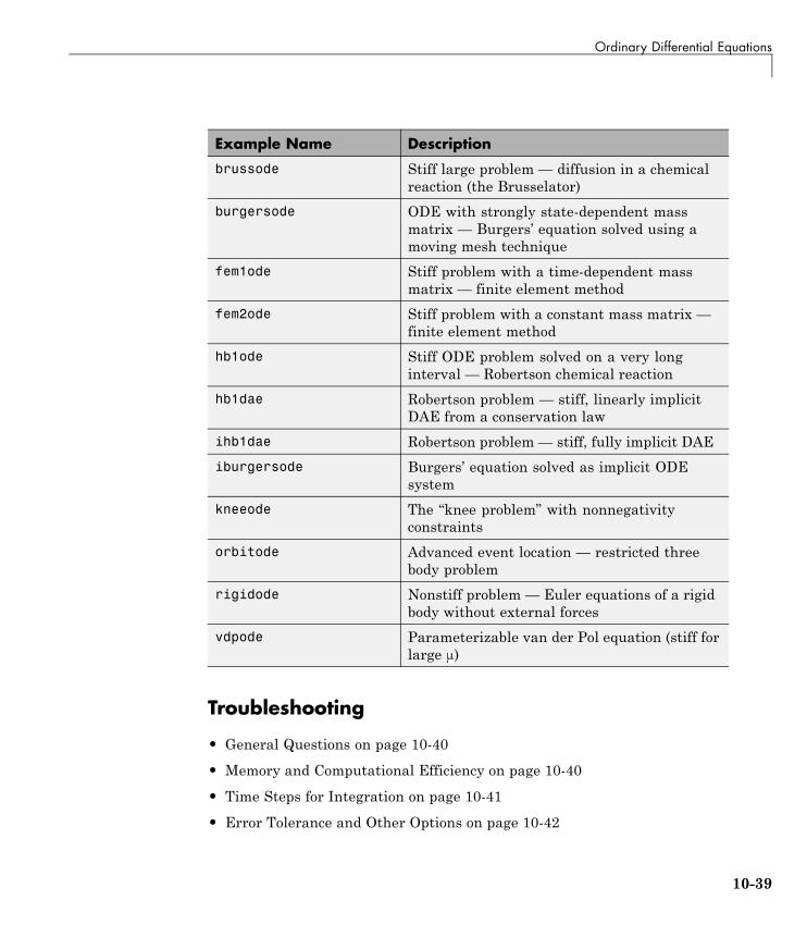
Ordinary Differential Equations
Example Name Description
brussode Stiff large problem — diffusion in a chemicalreaction (the Brusselator)
burgersode ODE with strongly state-dependent massmatrix — Burgers’ equation solved using amoving mesh technique
fem1ode Stiff problem with a time-dependent massmatrix — finite element method
fem2ode Stiff problem with a constant mass matrix —finite element method
hb1ode Stiff ODE problem solved on a very longinterval — Robertson chemical reaction
hb1dae Robertson problem — stiff, linearly implicitDAE from a conservation law
ihb1dae Robertson problem — stiff, fully implicit DAE
iburgersode Burgers’ equation solved as implicit ODEsystem
kneeode The “knee problem” with nonnegativityconstraints
orbitode Advanced event location — restricted threebody problem
rigidode Nonstiff problem — Euler equations of a rigidbody without external forces
vdpode Parameterizable van der Pol equation (stiff forlarge )
Troubleshooting
• General Questions on page 10-40
• Memory and Computational Efficiency on page 10-40
• Time Steps for Integration on page 10-41
• Error Tolerance and Other Options on page 10-42
10-39
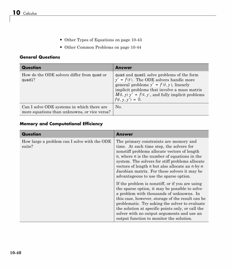
10 Calculus
• Other Types of Equations on page 10-43
• Other Common Problems on page 10-44
General Questions
Question Answer
How do the ODE solvers differ from quad orquadl?
quad and quadl solve problems of the form. The ODE solvers handle more
general problems , linearlyimplicit problems that involve a mass matrix
, and fully implicit problems.
Can I solve ODE systems in which there aremore equations than unknowns, or vice versa?
No.
Memory and Computational Efficiency
Question Answer
How large a problem can I solve with the ODEsuite?
The primary constraints are memory andtime. At each time step, the solvers fornonstiff problems allocate vectors of lengthn, where n is the number of equations in thesystem. The solvers for stiff problems allocatevectors of length n but also allocate an n-by-nJacobian matrix. For these solvers it may beadvantageous to use the sparse option.
If the problem is nonstiff, or if you are usingthe sparse option, it may be possible to solvea problem with thousands of unknowns. Inthis case, however, storage of the result can beproblematic. Try asking the solver to evaluatethe solution at specific points only, or call thesolver with no output arguments and use anoutput function to monitor the solution.
10-40
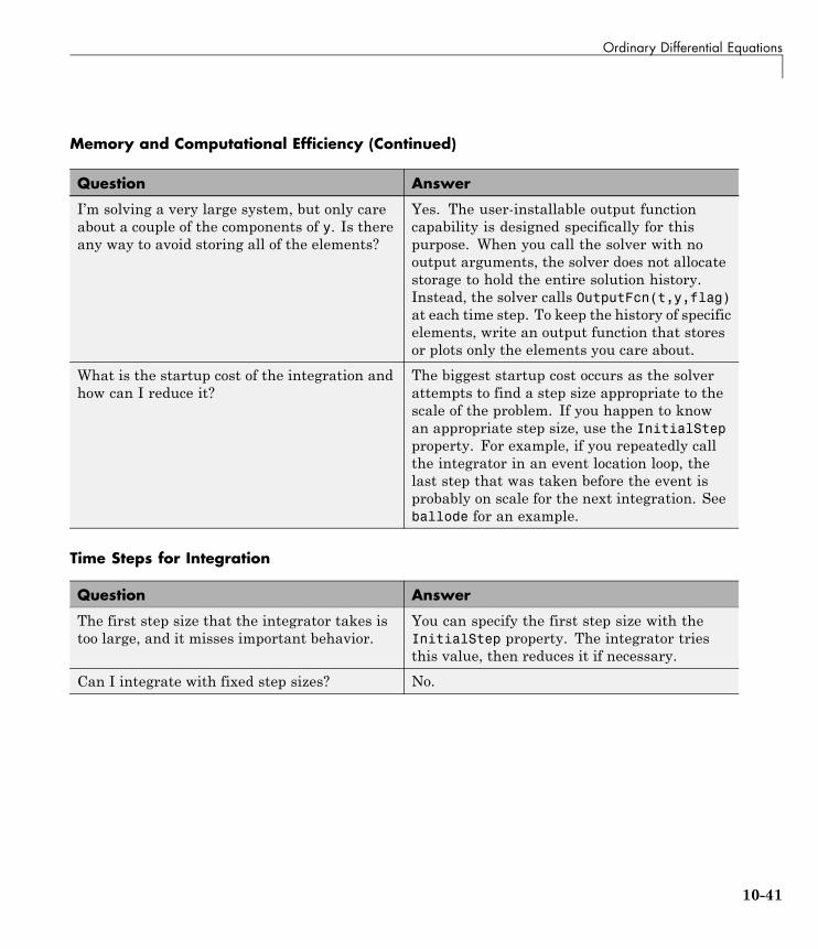
Ordinary Differential Equations
Memory and Computational Efficiency (Continued)
Question Answer
I’m solving a very large system, but only careabout a couple of the components of y. Is thereany way to avoid storing all of the elements?
Yes. The user-installable output functioncapability is designed specifically for thispurpose. When you call the solver with nooutput arguments, the solver does not allocatestorage to hold the entire solution history.Instead, the solver calls OutputFcn(t,y,flag)at each time step. To keep the history of specificelements, write an output function that storesor plots only the elements you care about.
What is the startup cost of the integration andhow can I reduce it?
The biggest startup cost occurs as the solverattempts to find a step size appropriate to thescale of the problem. If you happen to knowan appropriate step size, use the InitialStepproperty. For example, if you repeatedly callthe integrator in an event location loop, thelast step that was taken before the event isprobably on scale for the next integration. Seeballode for an example.
Time Steps for Integration
Question Answer
The first step size that the integrator takes istoo large, and it misses important behavior.
You can specify the first step size with theInitialStep property. The integrator triesthis value, then reduces it if necessary.
Can I integrate with fixed step sizes? No.
10-41

10 Calculus
Error Tolerance and Other Options
Question Answer
How do I choose RelTol and AbsTol? RelTol, the relative accuracy tolerance,controls the number of correct digits in theanswer. AbsTol, the absolute error tolerance,controls the difference between the answerand the solution. At each step, the error e incomponent i of the solution satisfies
|e(i)| max(RelTol*abs(y(i)),AbsTol(i))
Roughly speaking, this means that you wantRelTol correct digits in all solution componentsexcept those smaller than thresholdsAbsTol(i). Even if you are not interested in acomponent y(i) when it is small, you may haveto specify AbsTol(i) small enough to get somecorrect digits in y(i) so that you can accuratelycompute more interesting components.
I want answers that are correct to the precisionof the computer. Why can’t I simply set RelTolto eps?
You can get close to machine precision, but notthat close. The solvers do not allow RelTolnear eps because they try to approximate acontinuous function. At tolerances comparableto eps, the machine arithmetic causes allfunctions to look discontinuous.
How do I tell the solver that I don’t care aboutgetting an accurate answer for one of thesolution components?
You can increase the absolute error tolerancecorresponding to this solution component. Ifthe tolerance is bigger than the component, thisspecifies no correct digits for the component.The solver may have to get some correctdigits in this component to compute othercomponents accurately, but it generallyhandles this automatically.
10-42
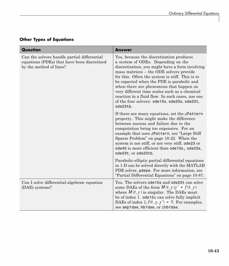
Ordinary Differential Equations
Other Types of Equations
Question Answer
Can the solvers handle partial differentialequations (PDEs) that have been discretizedby the method of lines?
Yes, because the discretization producesa system of ODEs. Depending on thediscretization, you might have a form involvingmass matrices – the ODE solvers providefor this. Often the system is stiff. This is tobe expected when the PDE is parabolic andwhen there are phenomena that happen onvery different time scales such as a chemicalreaction in a fluid flow. In such cases, use oneof the four solvers: ode15s, ode23s, ode23t,ode23tb.
If there are many equations, set the JPatternproperty. This might make the differencebetween success and failure due to thecomputation being too expensive. For anexample that uses JPattern, see “Large StiffSparse Problem” on page 10-22. When thesystem is not stiff, or not very stiff, ode23 orode45 is more efficient than ode15s, ode23s,ode23t, or ode23tb.
Parabolic-elliptic partial differential equationsin 1-D can be solved directly with the MATLABPDE solver, pdepe. For more information, see“Partial Differential Equations” on page 10-87.
Can I solve differential-algebraic equation(DAE) systems?
Yes. The solvers ode15s and ode23t can solvesome DAEs of the formwhere is singular. The DAEs mustbe of index 1. ode15i can solve fully implicitDAEs of index 1, . For examples,see amp1dae, hb1dae, or ihb1dae.
10-43
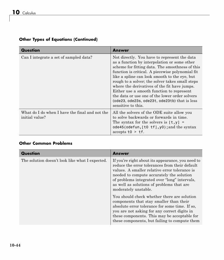
10 Calculus
Other Types of Equations (Continued)
Question Answer
Can I integrate a set of sampled data? Not directly. You have to represent the dataas a function by interpolation or some otherscheme for fitting data. The smoothness of thisfunction is critical. A piecewise polynomial fitlike a spline can look smooth to the eye, butrough to a solver; the solver takes small stepswhere the derivatives of the fit have jumps.Either use a smooth function to representthe data or use one of the lower order solvers(ode23, ode23s, ode23t, ode23tb) that is lesssensitive to this.
What do I do when I have the final and not theinitial value?
All the solvers of the ODE suite allow youto solve backwards or forwards in time.The syntax for the solvers is [t,y] =ode45(odefun,[t0 tf],y0);and the syntaxaccepts t0 > tf.
Other Common Problems
Question Answer
The solution doesn’t look like what I expected. If you’re right about its appearance, you need toreduce the error tolerances from their defaultvalues. A smaller relative error tolerance isneeded to compute accurately the solutionof problems integrated over “long” intervals,as well as solutions of problems that aremoderately unstable.
You should check whether there are solutioncomponents that stay smaller than theirabsolute error tolerance for some time. If so,you are not asking for any correct digits inthese components. This may be acceptable forthese components, but failing to compute them
10-44
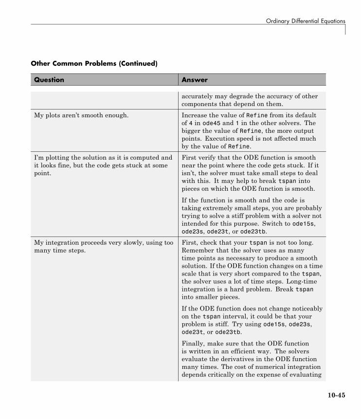
Ordinary Differential Equations
Other Common Problems (Continued)
Question Answer
accurately may degrade the accuracy of othercomponents that depend on them.
My plots aren’t smooth enough. Increase the value of Refine from its defaultof 4 in ode45 and 1 in the other solvers. Thebigger the value of Refine, the more outputpoints. Execution speed is not affected muchby the value of Refine.
I’m plotting the solution as it is computed andit looks fine, but the code gets stuck at somepoint.
First verify that the ODE function is smoothnear the point where the code gets stuck. If itisn’t, the solver must take small steps to dealwith this. It may help to break tspan intopieces on which the ODE function is smooth.
If the function is smooth and the code istaking extremely small steps, you are probablytrying to solve a stiff problem with a solver notintended for this purpose. Switch to ode15s,ode23s, ode23t, or ode23tb.
My integration proceeds very slowly, using toomany time steps.
First, check that your tspan is not too long.Remember that the solver uses as manytime points as necessary to produce a smoothsolution. If the ODE function changes on a timescale that is very short compared to the tspan,the solver uses a lot of time steps. Long-timeintegration is a hard problem. Break tspaninto smaller pieces.
If the ODE function does not change noticeablyon the tspan interval, it could be that yourproblem is stiff. Try using ode15s, ode23s,ode23t, or ode23tb.
Finally, make sure that the ODE functionis written in an efficient way. The solversevaluate the derivatives in the ODE functionmany times. The cost of numerical integrationdepends critically on the expense of evaluating
10-45
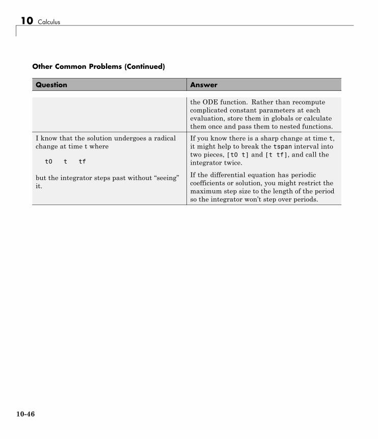
10 Calculus
Other Common Problems (Continued)
Question Answer
the ODE function. Rather than recomputecomplicated constant parameters at eachevaluation, store them in globals or calculatethem once and pass them to nested functions.
I know that the solution undergoes a radicalchange at time t where
t0 t tf
but the integrator steps past without “seeing”it.
If you know there is a sharp change at time t,it might help to break the tspan interval intotwo pieces, [t0 t] and [t tf], and call theintegrator twice.
If the differential equation has periodiccoefficients or solution, you might restrict themaximum step size to the length of the periodso the integrator won’t step over periods.
10-46
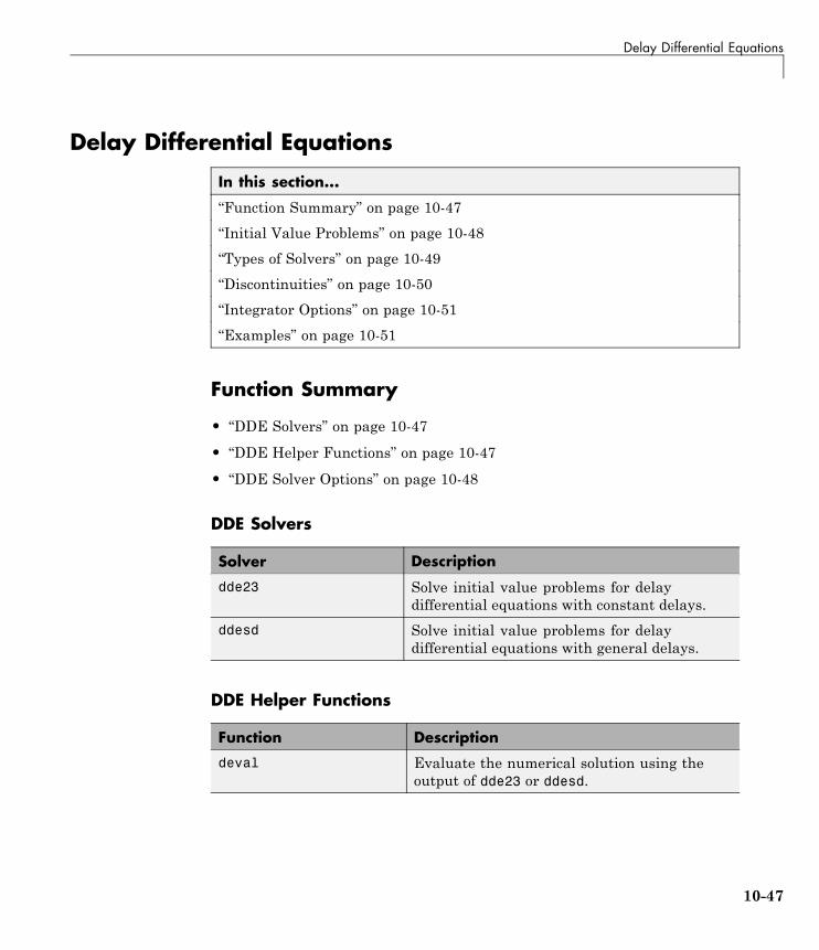
Delay Differential Equations
Delay Differential Equations
In this section...
“Function Summary” on page 10-47
“Initial Value Problems” on page 10-48
“Types of Solvers” on page 10-49
“Discontinuities” on page 10-50
“Integrator Options” on page 10-51
“Examples” on page 10-51
Function Summary
• “DDE Solvers” on page 10-47
• “DDE Helper Functions” on page 10-47
• “DDE Solver Options” on page 10-48
DDE Solvers
Solver Description
dde23 Solve initial value problems for delaydifferential equations with constant delays.
ddesd Solve initial value problems for delaydifferential equations with general delays.
DDE Helper Functions
Function Description
deval Evaluate the numerical solution using theoutput of dde23 or ddesd.
10-47
10 Calculus
DDE Solver OptionsUse these functions to create, alter, or access an options structure. An optionsstructure contains named properties, the values of which are passed to dde23or ddesd, thus affecting the solution of the problem.
Function Description
ddeset Create/alter the DDE options structure.
ddeget Extract properties from options structurecreated with ddeset.
Initial Value ProblemsThe DDE dde23 solver can solve systems of ordinary differential equations,such as
where is the independent variable, is the dependent variable, andrepresents (derivative of y with respect to t) . The delays (lags)are positive constants. The solver ddesd allows delays that depend on and .
History and Initial ValuesIn an initial value problem, you seek the solution on an interval with
. The DDE shows that depends on values of the solution at timesprior to . In particular, depends on . Because ofthis, a solution on depends on its values for , i.e., its history .
Propagation of DiscontinuitiesGenerally, the solution of an IVP for a system of DDEs has a jump in itsfirst derivative at the initial point because the first derivative of the historyfunction does not satisfy the DDE there. A discontinuity in any derivativepropagates into the future at spacings of when the delays areconstant, and in a more complicated way when they are not. For the DDEssolved by dde23 and ddesd, the solution becomes smoother as the integrationproceeds.
10-48
Delay Differential Equations
Types of SolversThis section describes:
• “DDE Solver dde23” on page 10-49
• “DDE Solver ddesd” on page 10-49
The basic syntax for the two solvers is shown in the function reference pagesfor dde23 and ddesd.
DDE Solver dde23The function dde23 solves initial value problems for DDEs with constantdelays. It integrates a system of first-order differential equations
on the interval , with and given history for .
dde23 produces a solution that is continuous on . You can use thefunction deval and the output of dde23 to evaluate the solution at specificpoints on the interval of integration.
dde23 tracks low-order discontinuities and integrates the differentialequations with the explicit Runge-Kutta (2,3) pair and interpolant used byode23. The Runge-Kutta formulas are implicit for step sizes longer than thedelays. When the solution is smooth enough that steps this big are justified,the implicit formulas are evaluated by a predictor-corrector iteration.
DDE Solver ddesdThe function ddesd solves initial value problems for DDEs with generaldelays. It integrates a system of first-order differential equations
on the interval , with , where delays can depend on bothand . Use the function deval and the output of ddesd to evaluate thesolution at specific points on the interval of integration.
10-49
10 Calculus
ddesd integrates with the classic four-stage, fourth-order explicit Runge-Kuttamethod, and controls the size of the residual of a natural interpolant. It usesiteration to take steps that are longer than the delays. For further details, see“Solving ODEs and DDEs with Residual Control,” L.F. Shampine, AppliedNumerical Mathematics, 52 (2005), pp 113-127.
Discontinuitiesdde23 performs better if it is informed of discontinuities in the history and atknown locations. Discontinuities may be specified by event functions. Thereis a property with which you can specify a solution that is different from thevalue given by the history function.
Discontinuity Property Comments
At the initial value InitialY Generally the initial valueis the value returnedby the history function, whichis to say that the solution iscontinuous at the initial point.However, if this is not the case,supply a different initial valueusing the InitialY property.
In the history, i.e.,the solution at ,or in the equationcoefficients for
Jumps Provide the known locations ofthe discontinuities in a vector asthe value of the Jumps property.Applies only to dde23.
State-dependent Events dde23 and ddesd use the eventsfunction you supply to locatethese discontinuities. When thesolver finds such a discontinuity,restart the integration tocontinue. Specify the solutionstructure for the currentintegration as the history forthe new integration. The solverextends each element of thesolution structure after eachrestart so that the final structure
10-50
Delay Differential Equations
Discontinuity Property Comments
provides the solution for thewhole interval of integration.If the new problem involves achange in the solution, use theInitialY property to specifythe initial value for the newintegration.
Integrator OptionsThe default integration properties in the DDE solver dde23 are selected tohandle common problems. In some cases, you can improve solver performanceby overriding these defaults. You do this by supplying dde23 with an optionsstructure that specifies one or more property values.
For example, to change the relative error tolerance of dde23 from the defaultvalue of 1e-3 to 1e-4,
1 Create an options structure using the function ddeset by entering
options = ddeset('RelTol', 1e-4);
2 Pass the options structure to dde23 as follows:
sol = dde23(ddefun,lags,history,tspan,options)
For a complete description of the available options, see the reference pagefor ddeset.
Examples
• “Constant Delay” on page 10-52
• “State-Dependent Delay” on page 10-54
• “Cardiovascular Model” on page 10-55
• “Additional Examples” on page 10-57
10-51
10 Calculus
Constant Delay
• “Solving the System” on page 10-52
• “Evaluating the Solution” on page 10-54
Solving the System. This example illustrates the straightforwardformulation, computation, and display of the solution of a system of DDEswith constant delays. The history is constant, which is often the case. Thedifferential equations are
The example solves the equations on [0,5] with history
for .
Note The demo ddex1 contains the complete code for this example. To seethe code in an editor, click the example name, or type edit ddex1 at thecommand line. To run the example type ddex1 at the command line.
1 Rewrite the problem as a first-order system. To use dde23, you mustrewrite the equations as an equivalent system of first-order differentialequations. Do this just as you would when solving IVPs and BVPs forODEs. However, this example needs no such preparation because it alreadyhas the form of a first-order system of equations.
2 Identify the lags. The delays (lags) are supplied to dde23 as avector. For the example we could use
lags = [1,0.2];
10-52
Delay Differential Equations
In coding the differential equations, = lags(j).
3 Code the system of first-order DDEs. Once you represent the equationsas a first-order system, and specify lags, you can code the equations as afunction that dde23 can use.
This code represents the system in the function, ddex1de.
function dydt = ddex1de(t,y,Z)ylag1 = Z(:,1);ylag2 = Z(:,2);dydt = [ylag1(1)
ylag1(1) + ylag2(2)y(2) ];
4 Code the history function. The history function for this example is
function S = ddex1hist(t)S = ones(3,1);
5 Apply the DDE solver. The example now calls dde23 with the functionsddex1de and ddex1hist.
sol = dde23(@ddex1de,lags,@ddex1hist,[0,5]);
Here the example supplies the interval of integration [0,5] directly.Because the history is constant, we could also call dde23 by
sol = dde23(@ddex1de,lags,ones(3,1),[0,5]);
6 View the results. Complete the example by displaying the results. dde23returns the mesh it selects and the solution there as fields in the solutionstructure sol. Often, these provide a smooth graph.
plot(sol.x,sol.y);title('An example of Wille'' and Baker');xlabel('time t');ylabel('solution y');legend('y_1','y_2','y_3',2)
10-53
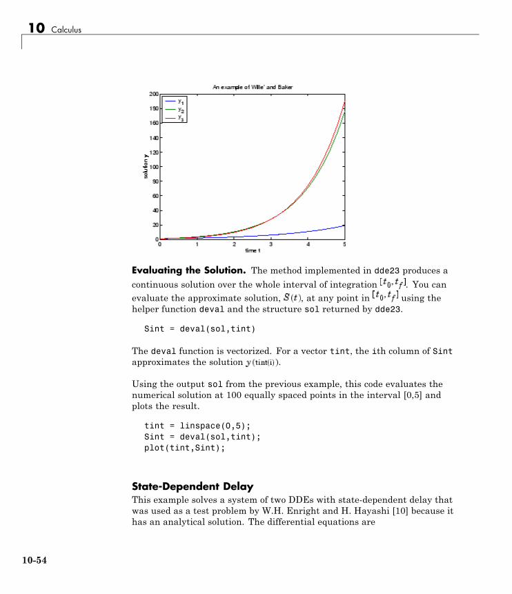
10 Calculus
Evaluating the Solution. The method implemented in dde23 produces a
continuous solution over the whole interval of integration . You canevaluate the approximate solution, , at any point in using thehelper function deval and the structure sol returned by dde23.
Sint = deval(sol,tint)
The deval function is vectorized. For a vector tint, the ith column of Sintapproximates the solution .
Using the output sol from the previous example, this code evaluates thenumerical solution at 100 equally spaced points in the interval [0,5] andplots the result.
tint = linspace(0,5);Sint = deval(sol,tint);plot(tint,Sint);
State-Dependent DelayThis example solves a system of two DDEs with state-dependent delay thatwas used as a test problem by W.H. Enright and H. Hayashi [10] because ithas an analytical solution. The differential equations are
10-54
Delay Differential Equations
The analytical solution
is used as the history for and the equations are solved on [0.1, 5].The only thing different about solving this example is that it must be solvedwith ddesd rather than dde23. This is because the first factor in the secondequation has the form with a delay that depends on the secondcomponent of the solution. The delay is provided to ddesd with a function like
function d = ddex3delay(t,y)% State dependent delay function for DDEX3d = exp(1 - y(2));
Note The demo ddex3 contains the complete code for this example. To seethe code in an editor, click the example name, or type edit ddex3 at thecommand line. To run the example type ddex3 at the command line.
Cardiovascular ModelThis example solves a cardiovascular model due to J. T. Ottesen [6]. Theequations are integrated over the interval [0,1000]. The situation of interestis when the peripheral pressure is reduced exponentially from its valueof 1.05 to 0.84 beginning at = 600.
This is a problem with one delay, a constant history, and three differentialequations with fourteen physical parameters. It has a discontinuity in a loworder derivative at t = 600.
Note The demo ddex2 contains the complete code for this example. To seethe code in an editor, click the example name, or type edit ddex2 at thecommand line. To run the example type ddex2 at the command line.
10-55
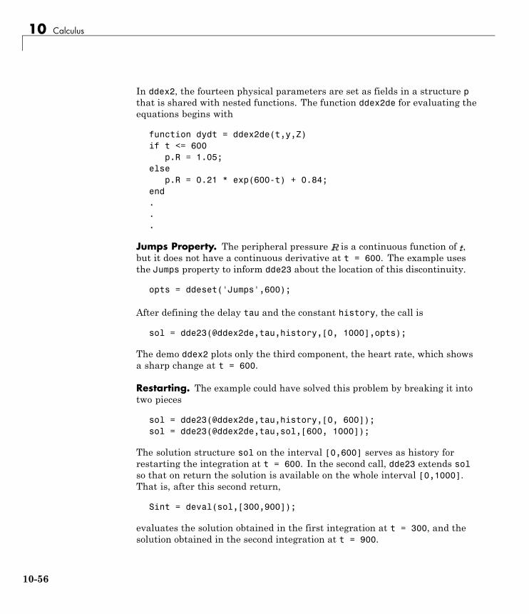
10 Calculus
In ddex2, the fourteen physical parameters are set as fields in a structure pthat is shared with nested functions. The function ddex2de for evaluating theequations begins with
function dydt = ddex2de(t,y,Z)if t <= 600
p.R = 1.05;else
p.R = 0.21 * exp(600-t) + 0.84;end...
Jumps Property. The peripheral pressure is a continuous function of ,but it does not have a continuous derivative at t = 600. The example usesthe Jumps property to inform dde23 about the location of this discontinuity.
opts = ddeset('Jumps',600);
After defining the delay tau and the constant history, the call is
sol = dde23(@ddex2de,tau,history,[0, 1000],opts);
The demo ddex2 plots only the third component, the heart rate, which showsa sharp change at t = 600.
Restarting. The example could have solved this problem by breaking it intotwo pieces
sol = dde23(@ddex2de,tau,history,[0, 600]);sol = dde23(@ddex2de,tau,sol,[600, 1000]);
The solution structure sol on the interval [0,600] serves as history forrestarting the integration at t = 600. In the second call, dde23 extends solso that on return the solution is available on the whole interval [0,1000].That is, after this second return,
Sint = deval(sol,[300,900]);
evaluates the solution obtained in the first integration at t = 300, and thesolution obtained in the second integration at t = 900.
10-56
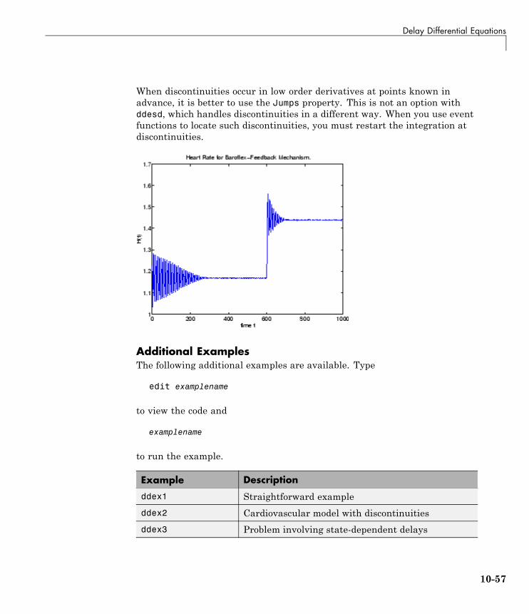
Delay Differential Equations
When discontinuities occur in low order derivatives at points known inadvance, it is better to use the Jumps property. This is not an option withddesd, which handles discontinuities in a different way. When you use eventfunctions to locate such discontinuities, you must restart the integration atdiscontinuities.
Additional ExamplesThe following additional examples are available. Type
edit examplename
to view the code and
examplename
to run the example.
Example Description
ddex1 Straightforward example
ddex2 Cardiovascular model with discontinuities
ddex3 Problem involving state-dependent delays
10-57

10 Calculus
Additional examples are provided by “Tutorial on Solving DDEs with DDE23,”available at http://www.mathworks.com/dde_tutorial.
10-58
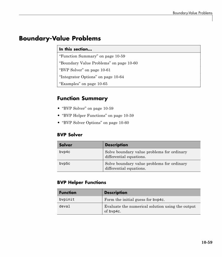
Boundary-Value Problems
Boundary-Value Problems
In this section...
“Function Summary” on page 10-59
“Boundary Value Problems” on page 10-60
“BVP Solver” on page 10-61
“Integrator Options” on page 10-64
“Examples” on page 10-65
Function Summary
• “BVP Solver” on page 10-59
• “BVP Helper Functions” on page 10-59
• “BVP Solver Options” on page 10-60
BVP Solver
Solver Description
bvp4c Solve boundary value problems for ordinarydifferential equations.
bvp5c Solve boundary value problems for ordinarydifferential equations.
BVP Helper Functions
Function Description
bvpinit Form the initial guess for bvp4c.
deval Evaluate the numerical solution using the outputof bvp4c.
10-59
10 Calculus
BVP Solver OptionsAn options structure contains named properties whose values are passedto bvp4c, and which affect problem solution. Use these functions to create,alter, or access an options structure.
Function Description
bvpset Create/alter the BVP options structure.
bvpget Extract properties from options structure createdwith bvpset.
Boundary Value ProblemsThe BVP solver is designed to handle systems of ordinary differentialequations
where x is the independent variable, y is the dependent variable, and y′represents the derivative of y with respect to x dy/dx.
See “First Order ODEs” on page 10-4 for general information about ODEs.
Boundary ConditionsIn a boundary value problem, the solution of interest satisfies certainboundary conditions. These conditions specify a relationship between thevalues of the solution at more than one x. In its basic syntax, bvp4c isdesigned to solve two-point BVPs, i.e., problems where the solution sought onan interval [a, b] must satisfy the boundary conditions
Unlike initial value problems, a boundary value problem may not have asolution, may have a finite number of solutions, or may have infinitely manysolutions. As an integral part of the process of solving a BVP, you need toprovide a guess for the required solution. The quality of this guess can becritical for the solver performance and even for a successful computation.
10-60
Boundary-Value Problems
There may be other difficulties when solving BVPs, such as problems imposedon infinite intervals or problems that involve singular coefficients. OftenBVPs involve unknown parameters p that have to be determined as partof solving the problem
In this case, the boundary conditions must suffice to determine the value of p.
BVP Solver
• “The BVP Solver” on page 10-61
• “BVP Solver Syntax” on page 10-62
• “BVP Solver Options” on page 10-64
The BVP SolverThe function bvp4c solves two-point boundary value problems for ordinarydifferential equations (ODEs). It integrates a system of first-order ordinarydifferential equations
on the interval , subject to general two-point boundary conditions
It can also accommodate other types of BVP problems, such as those that haveany of the following:
• Unknown parameters
• Singularities in the solutions
• Multipoint conditions
In this case, the number of boundary conditions must be sufficient todetermine the solution and the unknown parameters.
10-61
10 Calculus
bvp4c produces a solution that is continuous on and has a continuousfirst derivative there. You can use the function deval and the output of bvp4cto evaluate the solution at specific points on the interval of integration.
bvp4c is a finite difference code that implements the 3-stage Lobatto IIIaformula. This is a collocation formula and the collocation polynomial providesa C1-continuous solution that is fourth-order accurate uniformly in theinterval of integration. Mesh selection and error control are based on theresidual of the continuous solution.
The collocation technique uses a mesh of points to divide the interval ofintegration into subintervals. The solver determines a numerical solution bysolving a global system of algebraic equations resulting from the boundaryconditions, and the collocation conditions imposed on all the subintervals. Thesolver then estimates the error of the numerical solution on each subinterval.If the solution does not satisfy the tolerance criteria, the solver adapts themesh and repeats the process. The user must provide the points of the initialmesh as well as an initial approximation of the solution at the mesh points.
BVP Solver SyntaxThe basic syntax of the BVP solver is
sol = bvp4c(odefun,bcfun,solinit)
The input arguments are
odefun Handle to a function that evaluates the differentialequations. It has the basic form
dydx = odefun(x,y)
where x is a scalar, and dydx and y are column vectors.See “Function Handles” in MATLAB ProgrammingFundamentals for more information. odefun can alsoaccept a vector of unknown parameters and a variablenumber of known parameters, (see “BVP Solver Options”on page 10-64).
10-62
Boundary-Value Problems
bcfun Handle to a function that evaluates the residual in theboundary conditions. It has the basic form
res = bcfun(ya,yb)
where ya and yb are column vectors representing y(a) andy(b), and res is a column vector of the residual in satisfyingthe boundary conditions. bcfun can also accept a vectorof unknown parameters and a variable number of knownparameters, (see “BVP Solver Options” on page 10-64).
solinit Structure with fields x and y:
x Ordered nodes of the initial mesh. Boundaryconditions are imposed at a = solinit.x(1)and b = solinit.x(end).
y Initial guess for the solution withsolinit.y(:,i) a guess for the solution atthe node solinit.x(i).
The structure can have any name, but the fields must benamed x and y. It can also contain a vector that providesan initial guess for unknown parameters. You can formsolinit with the helper function bvpinit. See the bvpinitreference page for details.
The output argument sol is a structure created by the solver. In the basiccase the structure has fields x, y, yp, and solver.
sol.x Nodes of the mesh selected by bvp4c
sol.y Approximation to at the mesh points of sol.x
sol.yp Approximation to at the mesh points of sol.x
sol.solver 'bvp4c'
The structure sol returned by bvp4c contains an additional field if theproblem involves unknown parameters:
10-63
10 Calculus
sol.parameters Value of unknown parameters, if present, found by thesolver.
The function deval uses the output structure sol to evaluate the numericalsolution at any point from [a,b].
BVP Solver OptionsFor more advanced applications, you can specify solver options by passingan input argument options.
options Structure of optional parameters that change the defaultintegration properties. This is the fourth input argument.
sol = bvp4c(odefun,bcfun,solinit,options)
You can create the structure options using the functionbvpset. The bvpset reference page describes theproperties you can specify.
Integrator OptionsThe default integration properties in the BVP solver bvp4c are selected tohandle common problems. In some cases, you can improve solver performanceby overriding these defaults. You do this by supplying bvp4c with an optionsstructure that specifies one or more property values.
For example, to change the value of the relative error tolerance of bvp4cfrom the default value of 1e-3 to 1e-4,
1 Create an options structure using the function bvpset by entering
options = bvpset('RelTol', 1e-4);
2 Pass the options structure to bvp4c as follows:
sol = bvp4c(odefun,bcfun,solinit,options)
10-64
Boundary-Value Problems
For a complete description of the available options, see the reference pagefor bvpset.
Examples
• “Mathieu’s Equation” on page 10-65
• “Continuation” on page 10-69
• “Singular BVPs” on page 10-77
• “Multipoint BVPs” on page 10-81
• “Additional Examples” on page 10-85
Mathieu’s Equation
• “Solving the Problem” on page 10-65
• “Finding Unknown Parameters” on page 10-69
• “Evaluating the Solution” on page 10-69
Solving the Problem. This example determines the fourth eigenvalue ofMathieu’s Equation. It illustrates how to write second-order differentialequations as a system of two first-order ODEs and how to use bvp4c todetermine an unknown parameter .
The task is to compute the fourth ( ) eigenvalue lambda of Mathieu’sequation
Because the unknown parameter is present, this second-order differentialequation is subject to three boundary conditions
10-65
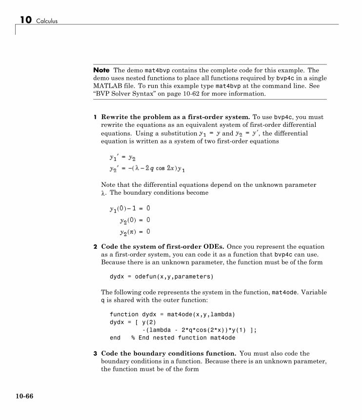
10 Calculus
Note The demo mat4bvp contains the complete code for this example. Thedemo uses nested functions to place all functions required by bvp4c in a singleMATLAB file. To run this example type mat4bvp at the command line. See“BVP Solver Syntax” on page 10-62 for more information.
1 Rewrite the problem as a first-order system. To use bvp4c, you mustrewrite the equations as an equivalent system of first-order differentialequations. Using a substitution and , the differentialequation is written as a system of two first-order equations
Note that the differential equations depend on the unknown parameter. The boundary conditions become
2 Code the system of first-order ODEs. Once you represent the equationas a first-order system, you can code it as a function that bvp4c can use.Because there is an unknown parameter, the function must be of the form
dydx = odefun(x,y,parameters)
The following code represents the system in the function, mat4ode. Variableq is shared with the outer function:
function dydx = mat4ode(x,y,lambda)dydx = [ y(2)
-(lambda - 2*q*cos(2*x))*y(1) ];end % End nested function mat4ode
3 Code the boundary conditions function. You must also code theboundary conditions in a function. Because there is an unknown parameter,the function must be of the form
10-66
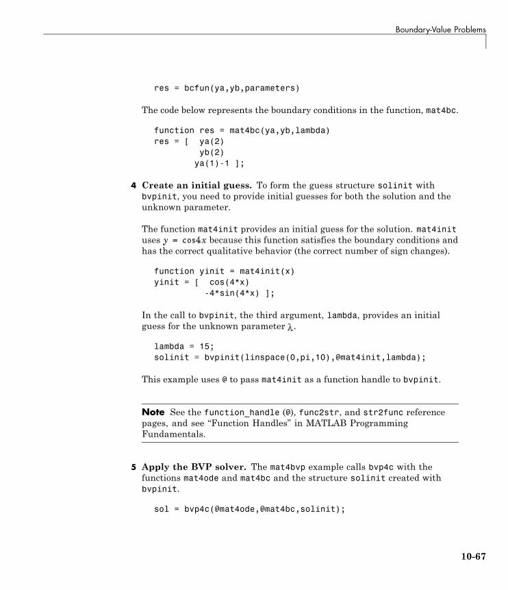
Boundary-Value Problems
res = bcfun(ya,yb,parameters)
The code below represents the boundary conditions in the function, mat4bc.
function res = mat4bc(ya,yb,lambda)res = [ ya(2)
yb(2)ya(1)-1 ];
4 Create an initial guess. To form the guess structure solinit withbvpinit, you need to provide initial guesses for both the solution and theunknown parameter.
The function mat4init provides an initial guess for the solution. mat4inituses because this function satisfies the boundary conditions andhas the correct qualitative behavior (the correct number of sign changes).
function yinit = mat4init(x)yinit = [ cos(4*x)
-4*sin(4*x) ];
In the call to bvpinit, the third argument, lambda, provides an initialguess for the unknown parameter .
lambda = 15;solinit = bvpinit(linspace(0,pi,10),@mat4init,lambda);
This example uses @ to pass mat4init as a function handle to bvpinit.
Note See the function_handle (@), func2str, and str2func referencepages, and see “Function Handles” in MATLAB ProgrammingFundamentals.
5 Apply the BVP solver. The mat4bvp example calls bvp4c with thefunctions mat4ode and mat4bc and the structure solinit created withbvpinit.
sol = bvp4c(@mat4ode,@mat4bc,solinit);
10-67

10 Calculus
6 View the results. Complete the example by displaying the results:
a Print the value of the unknown parameter found by bvp4c.
fprintf('Fourth eigenvalue is approximately %7.3f.\n',...sol.parameters)
b Use deval to evaluate the numerical solution at 100 equally spacedpoints in the interval , and plot its first component. This componentapproximates .
xint = linspace(0,pi);Sxint = deval(sol,xint);plot(xint,Sxint(1,:))axis([0 pi -1 1.1])title('Eigenfunction of Mathieu''s equation.')xlabel('x')ylabel('solution y')
The following plot shows the eigenfunction associated with the finaleigenvalue = 17.097.
10-68
Boundary-Value Problems
Finding Unknown Parameters. The bvp4c solver can find unknownparameters for problems of the form
You must provide bvp4c an initial guess for any unknown parameters in thevector solinit.parameters. When you call bvpinit to create the structuresolinit, specify the initial guess as a vector in the additional argumentparameters.
solinit = bvpinit(x,v,parameters)
The bvp4c function arguments odefun and bcfun must each have a thirdargument.
dydx = odefun(x,y,parameters)res = bcfun(ya,yb,parameters)
While solving the differential equations, bvp4c adjusts the value of unknownparameters to satisfy the boundary conditions. The solver returns the finalvalues of these unknown parameters in sol.parameters.
Evaluating the Solution. The collocation method implemented in bvp4cproduces a C1-continuous solution over the whole interval of integration .You can evaluate the approximate solution, , at any point in usingthe helper function deval and the structure sol returned by bvp4c.
Sxint = deval(sol,xint)
The deval function is vectorized. For a vector xint, the ith column of Sxintapproximates the solution .
Continuation
• “Introduction” on page 10-70
• “Using Continuation to Solve a BVP” on page 10-70
• “Using Continuation to Verify Consistency” on page 10-73
10-69
10 Calculus
Introduction. To solve a boundary value problem, you need to provide aninitial guess for the solution. The quality of your initial guess can be critical tothe solver performance, and to being able to solve the problem at all. However,coming up with a sufficiently good guess can be the most challenging part ofsolving a boundary value problem. Certainly, you should apply the knowledgeof the problem’s physical origin. Often a problem can be solved as a sequenceof relatively simpler problems, i.e., a continuation.
This example shows how to use continuation to:
• Solve a difficult BVP
• Verify a solution’s consistent behavior
Using Continuation to Solve a BVP. This example solves the differentialequation
for , on the interval [-1 1], with boundary conditions and. For , the solution has a transition layer at . Because of
this rapid change in the solution for small values of , the problem becomesdifficult to solve numerically.
The example solves the problem as a sequence of relatively simpler problems,i.e., a continuation. The solution of one problem is used as the initial guessfor solving the next problem.
Note The demo shockbvp contains the complete code for this example.The demo uses nested functions to place all required functions in a singleMATLAB file. To run this example type shockbvp at the command line.
Note This problem appears in [1] to illustrate the mesh selection capabilityof a well established BVP code COLSYS.
10-70
Boundary-Value Problems
1 Code the ODE and boundary condition functions. Code thedifferential equation and the boundary conditions as functions that bvp4ccan use:
The code below represents the differential equation and the boundaryconditions in the functions shockODE and shockBC. Note that shockODE isvectorized to improve solver performance. The additional parameter isrepresented by e and is shared with the outer function.
function dydx = shockODE(x,y)pix = pi*x;dydx = [ y(2,:)
-x/e.*y(2,:) - pi^2*cos(pix) - pix/e.*sin(pix) ];end % End nested function shockODE
function res = shockBC(ya,yb)res = [ ya(1)+2
yb(1) ];end % End nested function shockBC
2 Provide analytical partial derivatives. For this problem, the solverbenefits from using analytical partial derivatives. The code belowrepresents the derivatives in functions shockJac and shockBCJac.
function jac = shockJac(x,y)jac = [ 0 1
0 -x/e ];end % End nested function shockJac
function [dBCdya,dBCdyb] = shockBCJac(ya,yb)dBCdya = [ 1 0
0 0 ];dBCdyb = [ 0 0
1 0 ];end % End nested function shockBCJac
shockJac shares e with the outer function.
Tell bvp4c to use these functions to evaluate the partial derivatives bysetting the options FJacobian and BCJacobian. Also set 'Vectorized'
10-71
10 Calculus
to 'on' to indicate that the differential equation function shockODE isvectorized.
options = bvpset('FJacobian',@shockJac,...'BCJacobian',@shockBCJac,...'Vectorized','on');
3 Create an initial guess. You must provide bvp4c with a guess structurethat contains an initial mesh and a guess for values of the solution at themesh points. A constant guess of and , and a mesh of fiveequally spaced points on [-1 1] suffice to solve the problem for .Use bvpinit to form the guess structure.
sol = bvpinit([-1 -0.5 0 0.5 1],[1 0]);
4 Use continuation to solve the problem. To obtain the solution for theparameter , the example uses continuation by solving a sequence
of problems for . The solver bvp4c does not performcontinuation automatically, but the code’s user interface has been designedto make continuation easy. The code uses the output sol that bvp4cproduces for one value of e as the guess in the next iteration.
e = 0.1;for i=2:4
e = e/10;sol = bvp4c(@shockODE,@shockBC,sol,options);
end
5 View the results. Complete the example by displaying the final solution
plot(sol.x,sol.y(1,:))axis([-1 1 -2.2 2.2])title(['There is a shock at x = 0 when \epsilon = '...
sprintf('%.e',e) '.'])xlabel('x')ylabel('solution y')
10-72
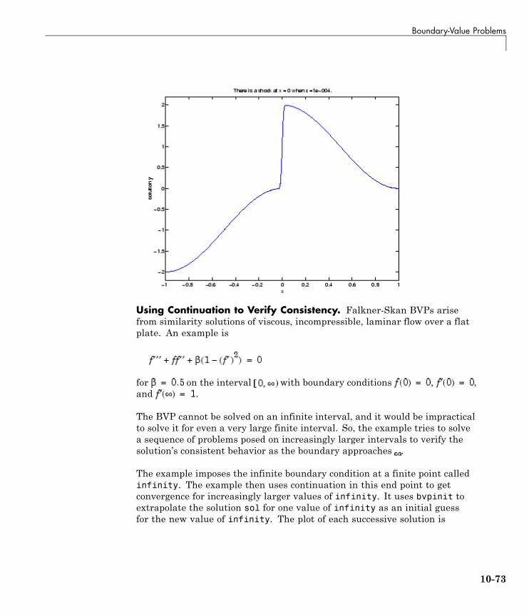
Boundary-Value Problems
Using Continuation to Verify Consistency. Falkner-Skan BVPs arisefrom similarity solutions of viscous, incompressible, laminar flow over a flatplate. An example is
for on the interval with boundary conditions , ,and .
The BVP cannot be solved on an infinite interval, and it would be impracticalto solve it for even a very large finite interval. So, the example tries to solvea sequence of problems posed on increasingly larger intervals to verify thesolution’s consistent behavior as the boundary approaches .
The example imposes the infinite boundary condition at a finite point calledinfinity. The example then uses continuation in this end point to getconvergence for increasingly larger values of infinity. It uses bvpinit toextrapolate the solution sol for one value of infinity as an initial guessfor the new value of infinity. The plot of each successive solution is
10-73
10 Calculus
superimposed over those of previous solutions so they can easily be comparedfor consistency.
Note The demo fsbvp contains the complete code for this example. The demouses nested functions to place all required functions in a single MATLAB file.To run this example type fsbvp at the command line.
1 Code the ODE and boundary condition functions. Code thedifferential equation and the boundary conditions as functions that bvp4ccan use. The problem parameter beta is shared with the outer function.
function dfdeta = fsode(eta,f)dfdeta = [ f(2)
f(3)-f(1)*f(3) - beta*(1 - f(2)^2) ];
end % End nested function fsode
function res = fsbc(f0,finf)res = [f0(1)
f0(2)finf(2) - 1];
end % End nested function fsbc
2 Create an initial guess. You must provide bvp4c with a guess structurethat contains an initial mesh and a guess for values of the solution atthe mesh points. A crude mesh of five points and a constant guess thatsatisfies the boundary conditions are good enough to get convergence wheninfinity = 3.
infinity = 3;maxinfinity = 6;
solinit = bvpinit(linspace(0,infinity,5),[0 0 1]);
3 Solve on the initial interval. The example obtains the solution forinfinity = 3. It then prints the computed value of for comparisonwith the value reported by Cebeci and Keller [2]:
sol = bvp4c(@fsode,@fsbc,solinit);
10-74
Boundary-Value Problems
eta = sol.x;f = sol.y;
fprintf('\n');fprintf('Cebeci & Keller report that f''''(0) = 0.92768.\n')fprintf('Value computed using infinity = %g is %7.5f.\n', ...
infinity,f(3,1))
The example prints
Cebeci & Keller report that f''(0) = 0.92768.Value computed using infinity = 3 is 0.92915.
4 Setup the figure and plot the initial solution.
figureplot(eta,f(2,:),eta(end),f(2,end),'o');axis([0 maxinfinity 0 1.4]);title('Falkner-Skan equation, positive wall shear, ...
\beta = 0.5.')xlabel('\eta')ylabel('df/d\eta')hold ondrawnowshg
10-75
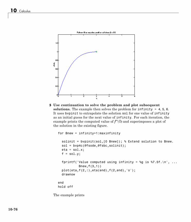
10 Calculus
5 Use continuation to solve the problem and plot subsequentsolutions. The example then solves the problem for infinity = 4, 5, 6.It uses bvpinit to extrapolate the solution sol for one value of infinityas an initial guess for the next value of infinity. For each iteration, theexample prints the computed value of and superimposes a plot ofthe solution in the existing figure.
for Bnew = infinity+1:maxinfinity
solinit = bvpinit(sol,[0 Bnew]); % Extend solution to Bnew.sol = bvp4c(@fsode,@fsbc,solinit);eta = sol.x;f = sol.y;
fprintf('Value computed using infinity = %g is %7.5f.\n', ...Bnew,f(3,1))
plot(eta,f(2,:),eta(end),f(2,end),'o');drawnow
endhold off
The example prints
10-76

Boundary-Value Problems
Value computed using infinity = 4 is 0.92774.Value computed using infinity = 5 is 0.92770.Value computed using infinity = 6 is 0.92770.
Note that the values approach 0.92768 as reported by Cebeci and Keller.The superimposed plots confirm the consistency of the solution’s behavior.
Singular BVPs
• “Introduction” on page 10-77
• “Emden’s equation” on page 10-78
Introduction. The function bvp4c solves a class of singular BVPs of the form
(10-1)
It can also accommodate unknown parameters for problems of the form
10-77
10 Calculus
Singular problems must be posed on an interval with . Use bvpsetto pass the constant matrix to bvp4c as the value of the 'SingularTerm'integration property. Boundary conditions at must be consistent withthe necessary condition for a smooth solution, . An initial guessshould also satisfy this necessary condition.
When you solve a singular BVP using
sol = bvp4c(@odefun,@bcfun,solinit,options)
bvp4c requires that your function odefun(x,y) return only the value of theterm in Equation 5-2.
Emden’s equation. Emden’s equation arises in modeling a spherical body ofgas. The PDE of the model is reduced by symmetry to the ODE
on an interval . The coefficient is singular at , but symmetryimplies the boundary condition . With this boundary condition,the term
is well-defined as approaches 0. For the boundary condition ,this BVP has the analytical solution
10-78
Boundary-Value Problems
Note The demo emdenbvp contains the complete code for this example. Thedemo uses subfunctions to place all required functions in a single MATLABfile. To run this example type emdenbvp at the command line.
1 Rewrite the problem as a first-order system and identify thesingular term. Using a substitution and , write thedifferential equation as a system of two first-order equations
The boundary conditions become
Writing the ODE system in a vector-matrix form
the terms of Equation 5-2 are identified as
and
10-79
10 Calculus
2 Code the ODE and boundary condition functions. Code thedifferential equation and the boundary conditions as functions that bvp4ccan use.
function dydx = emdenode(x,y)dydx = [ y(2)
-y(1)^5 ];function res = emdenbc(ya,yb)res = [ ya(2)
yb(1) - sqrt(3)/2 ];
3 Setup integration properties. Use the matrix as the value of the'SingularTerm' integration property.
S = [0,0;0,-2];options = bvpset('SingularTerm',S);
4 Create an initial guess. This example starts with a mesh of five pointsand a constant guess for the solution.
Use bvpinit to form the guess structure
guess = [sqrt(3)/2;0];solinit = bvpinit(linspace(0,1,5),guess);
5 Solve the problem. Use the standard bvp4c syntax to solve the problem.
sol = bvp4c(@emdenode,@emdenbc,solinit,options);
6 View the results. This problem has an analytical solution
The example evaluates the analytical solution at 100 equally spaced pointsand plots it along with the numerical solution computed using bvp4c.
10-80
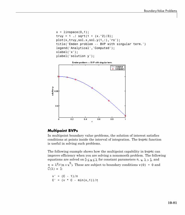
Boundary-Value Problems
x = linspace(0,1);truy = 1 ./ sqrt(1 + (x.^2)/3);plot(x,truy,sol.x,sol.y(1,:),'ro');title('Emden problem -- BVP with singular term.')legend('Analytical','Computed');xlabel('x');ylabel('solution y');
Multipoint BVPsIn multipoint boundary value problems, the solution of interest satisfiesconditions at points inside the interval of integration. The bvp4c functionis useful in solving such problems.
The following example shows how the multipoint capability in bvp4c canimprove efficiency when you are solving a nonsmooth problem. The followingequations are solved on for constant parameters n, , , and
. These are subject to boundary conditions v(0) = 0 and:
v' = (C - 1)/nC' = (v * C - min(x,1))/
10-81
10 Calculus
The term min(x,1) is not smooth at xc = 1, and this can affect the solver’sefficiency. By introducing an interface point at xc = 1, smooth solutions canbe obtained on [0,1] and [1, ]. To get a continuous solution over the entireinterval [0, ], the example imposes matching conditions at the interface.
Note The demo threebvp contains the complete code for this example andsolves the problem for = 2, n = 0.05, and several values of . The demouses nested functions to place all functions required by bvp4c in a singleMATLAB file and to communicate problem parameters efficiently. To run thisexample, type threebvp at the MATLAB command prompt.
The demo takes you through the following steps:
1 Determine the interfaces and divide the interval of integration intoregions. Introducing an interface point at xc = 1 divides the probleminto two regions in which the solutions remain smooth. The differentialequations for the two regions are
Region 1:
v' = (C - 1)/nC' = (v * C - x)/
Region 2:
v' = (C - 1)/nC' = (v * C - 1)/
Note that the interface xc = 1 is included in both regions. At xc = 1,bvp4c produces a left and right solution. These solutions are denoted asv(1-), C(1-) and v(1+), C(1+) respectively.
2 Determine the boundary conditions. Solving two first-order differentialequations in two regions requires imposing four boundary conditions. Twoof these conditions come from the original formulation; the others enforcethe continuity of the solution across the interface xc = 1:
v(0) = 0C( ) - 1 = 0
10-82
Boundary-Value Problems
v(1-) - v(1+) = 0C(1-) - C(1+) = 0
Here, v(1-), C(1-) and v(1+), C(1+) denote the left and right solutionat the interface.
3 Code the derivative function. In the derivative function, y(1)corresponds to v(x), and y(2) corresponds to C(x). The additional inputargument region identifies the region in which the derivative is evaluated.bvp4c enumerates regions from left to right, starting with 1. Note that theproblem parameters n and are shared with the outer function:
function dydx = f(x,y,region)dydx = zeros(2,1);dydx(1) = (y(2) - 1)/n;
% The definition of C'(x) depends on the region.switch region
case 1 % x in [0 1]dydx(2) = (y(1)*y(2) - x)/ ;
case 2 % x in [1 ]dydx(2) = (y(1)*y(2) - 1)/ ;
endend % End nested function f
4 Code the boundary conditions function. For multipoint BVPs,the arguments of the boundary conditions function, YL and YR, becomematrices. In particular, the kth column YL(:,k) represents the solutionat the left boundary of the kth region. Similarly, YR(:,k) represents thesolution at the right boundary of the kth region.
In the example, y(0) is approximated by YL(:,1), while y( ) isapproximated by YR(:,end). Continuity of the solution at the internalinterface requires that YR(:,1) = YL(:,2). Nested function bc computesthe residual in the boundary conditions:
function res = bc(YL,YR)res = [YL(1,1) % v(0) = 0
YR(1,1) - YL(1,2) % Continuity of v(x) at x=1YR(2,1) - YL(2,2) % Continuity of C(x) at x=1
10-83
10 Calculus
YR(2,end) - 1]; % C( ) = 1end % End nested function bc
5 Create an initial guess. For multipoint BVPs, when creating an initialguess using bvpinit, use double entries in xinit for the interface point xc.This example uses a constant guess yinit = [1;1]:
xc = 1;xinit = [0, 0.25, 0.5, 0.75, xc, xc, 1.25, 1.5, 1.75, 2];solinit = bvpinit(xinit,yinit)
For multipoint BVPs, you can use different guesses in different regions. Todo that, you specify the initial guess for y as a function using the followingsyntax:
solinit = bvpinit(xinit,@yinitfcn)
The initial guess function must have the following general form:
function y = yinitfcn(x,region)switch regioncase 1 % x in [0, 1]
y = [1;1]; % initial guess for y(x)case 2 % x in [1, ]
y = [1;1]; % initial guess for y(x),end
6 Apply the solver. The bvp4c function uses the same syntax for multipointBVPs as it does for two-point BVPs:
sol = bvp4c(@f,@bc,solinit);
The mesh points returned in sol.x are adapted to the solution behavior,but the mesh still includes a double entry for the interface point xc = 1.Corresponding columns of sol.y represent the left and right solution at xc.
7 View the results. Using deval, the solution can be evaluated at any pointin the interval of integration.
Note that, with the left and right values computed at the interface, thesolution is not uniquely defined at xc = 1. When evaluating the solution
10-84
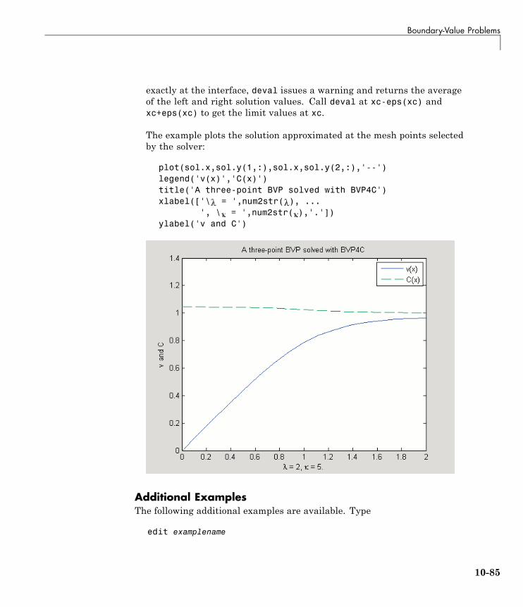
Boundary-Value Problems
exactly at the interface, deval issues a warning and returns the averageof the left and right solution values. Call deval at xc-eps(xc) andxc+eps(xc) to get the limit values at xc.
The example plots the solution approximated at the mesh points selectedby the solver:
plot(sol.x,sol.y(1,:),sol.x,sol.y(2,:),'--')legend('v(x)','C(x)')title('A three-point BVP solved with BVP4C')xlabel(['\ = ',num2str( ), ...
', \ = ',num2str( ),'.'])ylabel('v and C')
Additional ExamplesThe following additional examples are available. Type
edit examplename
10-85
10 Calculus
to view the code and
examplename
to run the example.
Example Name Description
emdenbvp Emden’s equation, a singular BVP
fsbvp Falkner-Skan BVP on an infinite interval
mat4bvp Fourth eigenfunction of Mathieu’s equation
shockbvp Solution with a shock layer near x = 0
twobvp BVP with exactly two solutions
threebvp Three-point boundary value problem
Additional examples are provided by “Tutorial on Solving BVPs with BVP4C,”available at http://www.mathworks.com/bvp_tutorial.
10-86
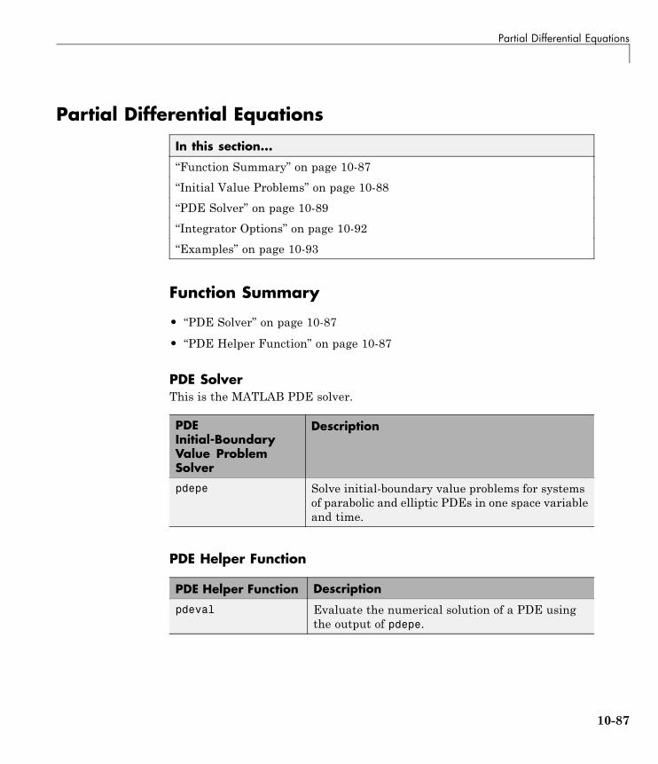
Partial Differential Equations
Partial Differential Equations
In this section...
“Function Summary” on page 10-87
“Initial Value Problems” on page 10-88
“PDE Solver” on page 10-89
“Integrator Options” on page 10-92
“Examples” on page 10-93
Function Summary
• “PDE Solver” on page 10-87
• “PDE Helper Function” on page 10-87
PDE SolverThis is the MATLAB PDE solver.
PDEInitial-BoundaryValue ProblemSolver
Description
pdepe Solve initial-boundary value problems for systemsof parabolic and elliptic PDEs in one space variableand time.
PDE Helper Function
PDE Helper Function Description
pdeval Evaluate the numerical solution of a PDE usingthe output of pdepe.
10-87
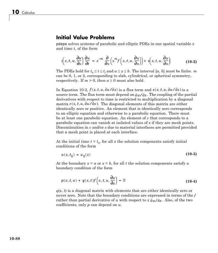
10 Calculus
Initial Value Problemspdepe solves systems of parabolic and elliptic PDEs in one spatial variable xand time t, of the form
(10-2)
The PDEs hold for t0 ≤ t ≤ tf and a ≤ x ≤ b. The interval [a, b] must be finite. mcan be 0, 1, or 2, corresponding to slab, cylindrical, or spherical symmetry,respectively. If m > 0, then a ≥ 0 must also hold.
In Equation 10-2, is a flux term and is asource term. The flux term must depend on . The coupling of the partialderivatives with respect to time is restricted to multiplication by a diagonalmatrix . The diagonal elements of this matrix are eitheridentically zero or positive. An element that is identically zero correspondsto an elliptic equation and otherwise to a parabolic equation. There mustbe at least one parabolic equation. An element of c that corresponds to aparabolic equation can vanish at isolated values of x if they are mesh points.Discontinuities in c and/or s due to material interfaces are permitted providedthat a mesh point is placed at each interface.
At the initial time t = t0, for all x the solution components satisfy initialconditions of the form
(10-3)
At the boundary x = a or x = b, for all t the solution components satisfy aboundary condition of the form
(10-4)
q(x, t) is a diagonal matrix with elements that are either identically zero ornever zero. Note that the boundary conditions are expressed in terms of the frather than partial derivative of u with respect to x . Also, of the twocoefficients, only p can depend on u.
10-88

Partial Differential Equations
PDE Solver
The PDE SolverThe MATLAB PDE solver, pdepe, solves initial-boundary value problems forsystems of parabolic and elliptic PDEs in the one space variable x and time t.There must be at least one parabolic equation in the system.
The pdepe solver converts the PDEs to ODEs using a second-order accuratespatial discretization based on a fixed set of user-specified nodes. Thediscretization method is described in [9]. The time integration is done withode15s. The pdepe solver exploits the capabilities of ode15s for solvingthe differential-algebraic equations that arise when Equation 10-2 containselliptic equations, and for handling Jacobians with a specified sparsitypattern. ode15s changes both the time step and the formula dynamically.
After discretization, elliptic equations give rise to algebraic equations. If theelements of the initial conditions vector that correspond to elliptic equationsare not “consistent” with the discretization, pdepe tries to adjust them beforebeginning the time integration. For this reason, the solution returned forthe initial time may have a discretization error comparable to that at anyother time. If the mesh is sufficiently fine, pdepe can find consistent initialconditions close to the given ones. If pdepe displays a message that it hasdifficulty finding consistent initial conditions, try refining the mesh. Noadjustment is necessary for elements of the initial conditions vector thatcorrespond to parabolic equations.
PDE Solver SyntaxThe basic syntax of the solver is:
sol = pdepe(m,pdefun,icfun,bcfun,xmesh,tspan)
Note Correspondences given are to terms used in “Initial Value Problems”on page 10-88.
The input arguments are
10-89
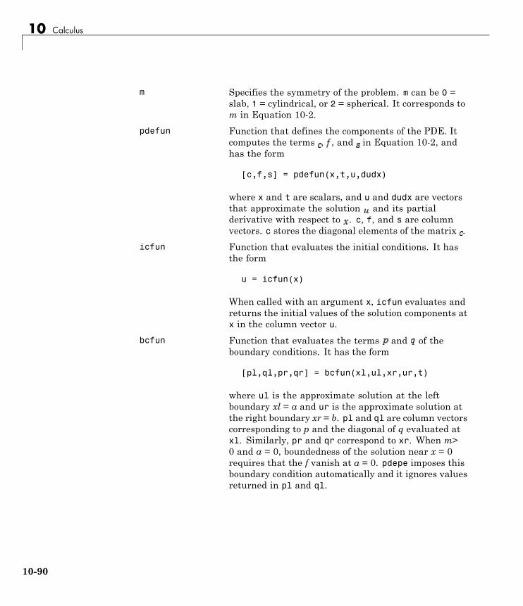
10 Calculus
m Specifies the symmetry of the problem. m can be 0 =slab, 1 = cylindrical, or 2 = spherical. It corresponds tom in Equation 10-2.
pdefun Function that defines the components of the PDE. Itcomputes the terms , , and in Equation 10-2, andhas the form
[c,f,s] = pdefun(x,t,u,dudx)
where x and t are scalars, and u and dudx are vectorsthat approximate the solution and its partialderivative with respect to . c, f, and s are columnvectors. c stores the diagonal elements of the matrix .
icfun Function that evaluates the initial conditions. It hasthe form
u = icfun(x)
When called with an argument x, icfun evaluates andreturns the initial values of the solution components atx in the column vector u.
bcfun Function that evaluates the terms and of theboundary conditions. It has the form
[pl,ql,pr,qr] = bcfun(xl,ul,xr,ur,t)
where ul is the approximate solution at the leftboundary xl = a and ur is the approximate solution atthe right boundary xr = b. pl and ql are column vectorscorresponding to p and the diagonal of q evaluated atxl. Similarly, pr and qr correspond to xr. When m>0 and a = 0, boundedness of the solution near x = 0requires that the f vanish at a = 0. pdepe imposes thisboundary condition automatically and it ignores valuesreturned in pl and ql.
10-90
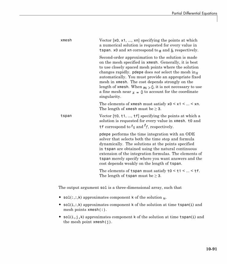
Partial Differential Equations
xmesh Vector [x0, x1, ..., xn] specifying the points at whicha numerical solution is requested for every value intspan. x0 and xn correspond to and , respectively.
Second-order approximation to the solution is madeon the mesh specified in xmesh. Generally, it is bestto use closely spaced mesh points where the solutionchanges rapidly. pdepe does not select the mesh inautomatically. You must provide an appropriate fixedmesh in xmesh. The cost depends strongly on thelength of xmesh. When , it is not necessary to usea fine mesh near to account for the coordinatesingularity.
The elements of xmesh must satisfy x0 < x1 < ... < xn.The length of xmesh must be ≥ 3.
tspan Vector [t0, t1, ..., tf] specifying the points at which asolution is requested for every value in xmesh. t0 andtf correspond to and , respectively.
pdepe performs the time integration with an ODEsolver that selects both the time step and formuladynamically. The solutions at the points specifiedin tspan are obtained using the natural continuousextension of the integration formulas. The elements oftspan merely specify where you want answers and thecost depends weakly on the length of tspan.
The elements of tspan must satisfy t0 < t1 < ... < tf.The length of tspan must be ≥ 3.
The output argument sol is a three-dimensional array, such that
• sol(:,:,k) approximates component k of the solution .
• sol(i,:,k) approximates component k of the solution at time tspan(i) andmesh points xmesh(:).
• sol(i,j,k) approximates component k of the solution at time tspan(i) andthe mesh point xmesh(j).
10-91

10 Calculus
PDE Solver OptionsFor more advanced applications, you can also specify as input argumentssolver options and additional parameters that are passed to the PDEfunctions.
options Structure of optional parameters that change thedefault integration properties. This is the seventh inputargument.
sol = pdepe(m,pdefun,icfun,bcfun,...xmesh,tspan,options)
See “Integrator Options” on page 10-92 for moreinformation.
Integrator OptionsThe default integration properties in the MATLAB PDE solver are selected tohandle common problems. In some cases, you can improve solver performanceby overriding these defaults. You do this by supplying pdepe with one or moreproperty values in an options structure.
sol = pdepe(m,pdefun,icfun,bcfun,xmesh,tspan,options)
Use odeset to create the options structure. Only those options of theunderlying ODE solver shown in the following table are available for pdepe.The defaults obtained by leaving off the input argument options aregenerally satisfactory. “Integrator Options” on page 10-9 tells you how tocreate the structure and describes the properties.
PDE Properties
Properties Category Property Name
Error control RelTol, AbsTol, NormControl
Step-size InitialStep, MaxStep
10-92
Partial Differential Equations
Examples
• “Single PDE” on page 10-93
• “System of PDEs” on page 10-98
• “Additional Examples” on page 10-103
Single PDE
• “Solving the Equation” on page 10-93
• “Evaluating the Solution” on page 10-98
Solving the Equation. This example illustrates the straightforwardformulation, solution, and plotting of the solution of a single PDE
This equation holds on an interval for times t ≥ 0. At , thesolution satisfies the initial condition
At and , the solution satisfies the boundary conditions
Note The demo pdex1 contains the complete code for this example. The demouses subfunctions to place all functions it requires in a single MATLAB file.To run the demo type pdex1 at the command line. See “PDE Solver Syntax”on page 10-89 for more information.
1 Rewrite the PDE. Write the PDE in the form
10-93
10 Calculus
This is the form shown in Equation 10-2 and expected by pdepe. See“Initial Value Problems” on page 10-88 for more information. For thisexample, the resulting equation is
with parameter and the terms
2 Code the PDE. Once you rewrite the PDE in the form shown above(Equation 10-2) and identify the terms, you can code the PDE in a functionthat pdepe can use. The function must be of the form
[c,f,s] = pdefun(x,t,u,dudx)
where c, f, and s correspond to the , , and terms. The code belowcomputes c, f, and s for the example problem.
function [c,f,s] = pdex1pde(x,t,u,DuDx)c = pi^2;f = DuDx;s = 0;
3 Code the initial conditions function. You must code the initialconditions in a function of the form
u = icfun(x)
The code below represents the initial conditions in the function pdex1ic.
10-94
Partial Differential Equations
function u0 = pdex1ic(x)u0 = sin(pi*x);
4 Code the boundary conditions function. You must also code theboundary conditions in a function of the form
[pl,ql,pr,qr] = bcfun(xl,ul,xr,ur,t)
The boundary conditions, written in the same form as Equation 10-4, are
and
The code below evaluates the components and of theboundary conditions in the function pdex1bc.
function [pl,ql,pr,qr] = pdex1bc(xl,ul,xr,ur,t)pl = ul;ql = 0;pr = pi * exp(-t);qr = 1;
In the function pdex1bc, pl and ql correspond to the left boundaryconditions ( ), and pr and qr correspond to the right boundarycondition .
5 Select mesh points for the solution. Before you use the MATLAB PDEsolver, you need to specify the mesh points at which you want pdepeto evaluate the solution. Specify the points as vectors t and x.
The vectors t and x play different roles in the solver (see “PDE Solver” onpage 10-89). In particular, the cost and the accuracy of the solution dependstrongly on the length of the vector x. However, the computation is muchless sensitive to the values in the vector t.
10-95

10 Calculus
This example requests the solution on the mesh produced by 20 equallyspaced points from the spatial interval [0,1] and five values of t from thetime interval [0,2].
x = linspace(0,1,20);t = linspace(0,2,5);
6 Apply the PDE solver. The example calls pdepe with m = 0, the functionspdex1pde, pdex1ic, and pdex1bc, and the mesh defined by x and t at whichpdepe is to evaluate the solution. The pdepe function returns the numericalsolution in a three-dimensional array sol, where sol(i,j,k) approximatesthe kth component of the solution, , evaluated at t(i) and x(j).
m = 0;sol = pdepe(m,@pdex1pde,@pdex1ic,@pdex1bc,x,t);
This example uses @ to pass pdex1pde, pdex1ic, and pdex1bc as functionhandles to pdepe.
Note See the function_handle (@), func2str, and str2func referencepages, and the @ section of MATLAB Programming Fundamentals forinformation about function handles.
7 View the results. Complete the example by displaying the results:
a Extract and display the first solution component. In this example, thesolution has only one component, but for illustrative purposes, theexample “extracts” it from the three-dimensional array. The surface plotshows the behavior of the solution.
u = sol(:,:,1);
surf(x,t,u)title('Numerical solution computed with 20 mesh points')xlabel('Distance x')ylabel('Time t')
10-96
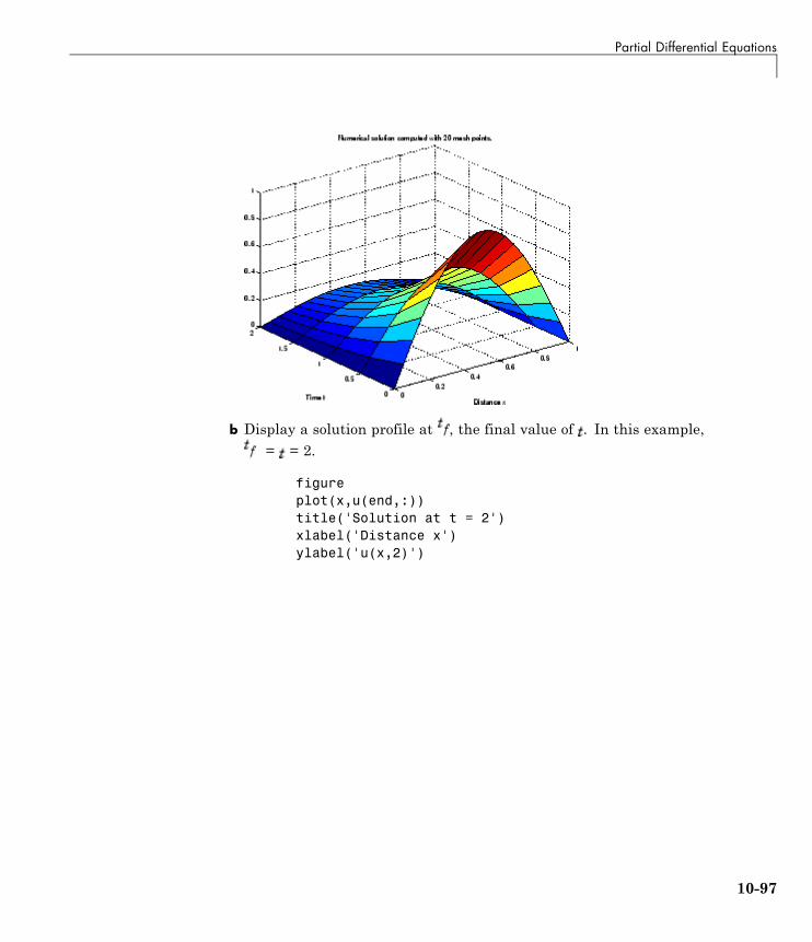
Partial Differential Equations
b Display a solution profile at , the final value of . In this example,= = 2.
figureplot(x,u(end,:))title('Solution at t = 2')xlabel('Distance x')ylabel('u(x,2)')
10-97
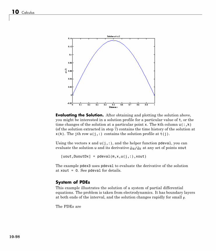
10 Calculus
Evaluating the Solution. After obtaining and plotting the solution above,you might be interested in a solution profile for a particular value of t, or thetime changes of the solution at a particular point x. The kth column u(:,k)(of the solution extracted in step 7) contains the time history of the solution atx(k). The jth row u(j,:) contains the solution profile at t(j).
Using the vectors x and u(j,:), and the helper function pdeval, you canevaluate the solution u and its derivative at any set of points xout
[uout,DuoutDx] = pdeval(m,x,u(j,:),xout)
The example pdex3 uses pdeval to evaluate the derivative of the solutionat xout = 0. See pdeval for details.
System of PDEsThis example illustrates the solution of a system of partial differentialequations. The problem is taken from electrodynamics. It has boundary layersat both ends of the interval, and the solution changes rapidly for small .
The PDEs are
10-98

Partial Differential Equations
where . The equations hold on an interval0 less than or equal to x less than or equal to 1 for times .
The solution satisfies the initial conditions
and boundary conditions
Note The demo pdex4 contains the complete code for this example. The demouses subfunctions to place all required functions in a single MATLAB file. Torun this example type pdex4 at the command line.
1 Rewrite the PDE. In the form expected by pdepe, the equations are
10-99
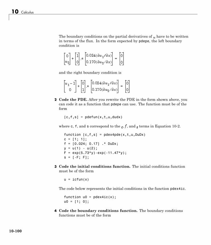
10 Calculus
The boundary conditions on the partial derivatives of have to be writtenin terms of the flux. In the form expected by pdepe, the left boundarycondition is
and the right boundary condition is
2 Code the PDE. After you rewrite the PDE in the form shown above, youcan code it as a function that pdepe can use. The function must be of theform
[c,f,s] = pdefun(x,t,u,dudx)
where c, f, and s correspond to the , , and terms in Equation 10-2.
function [c,f,s] = pdex4pde(x,t,u,DuDx)c = [1; 1];f = [0.024; 0.17] .* DuDx;y = u(1) - u(2);F = exp(5.73*y)-exp(-11.47*y);s = [-F; F];
3 Code the initial conditions function. The initial conditions functionmust be of the form
u = icfun(x)
The code below represents the initial conditions in the function pdex4ic.
function u0 = pdex4ic(x);u0 = [1; 0];
4 Code the boundary conditions function. The boundary conditionsfunctions must be of the form
10-100
Partial Differential Equations
[pl,ql,pr,qr] = bcfun(xl,ul,xr,ur,t)
The code below evaluates the components and (Equation10-4) of the boundary conditions in the function pdex4bc.
function [pl,ql,pr,qr] = pdex4bc(xl,ul,xr,ur,t)pl = [0; ul(2)];ql = [1; 0];pr = [ur(1)-1; 0];qr = [0; 1];
5 Select mesh points for the solution. The solution changes rapidly forsmall . The program selects the step size in time to resolve this sharpchange, but to see this behavior in the plots, output times must be selectedaccordingly. There are boundary layers in the solution at both ends of[0,1], so mesh points must be placed there to resolve these sharp changes.Often some experimentation is needed to select the mesh that reveals thebehavior of the solution.
x = [0 0.005 0.01 0.05 0.1 0.2 0.5 0.7 0.9 0.95 0.99 0.995 1];t = [0 0.005 0.01 0.05 0.1 0.5 1 1.5 2];
6 Apply the PDE solver. The example calls pdepe with m = 0, the functionspdex4pde, pdex4ic, and pdex4bc, and the mesh defined by x and t at whichpdepe is to evaluate the solution. The pdepe function returns the numericalsolution in a three-dimensional array sol, where sol(i,j,k) approximatesthe kth component of the solution, , evaluated at t(i) and x(j).
m = 0;sol = pdepe(m,@pdex4pde,@pdex4ic,@pdex4bc,x,t);
7 View the results. The surface plots show the behavior of the solutioncomponents.
u1 = sol(:,:,1);u2 = sol(:,:,2);
figuresurf(x,t,u1)title('u1(x,t)')xlabel('Distance x')
10-101
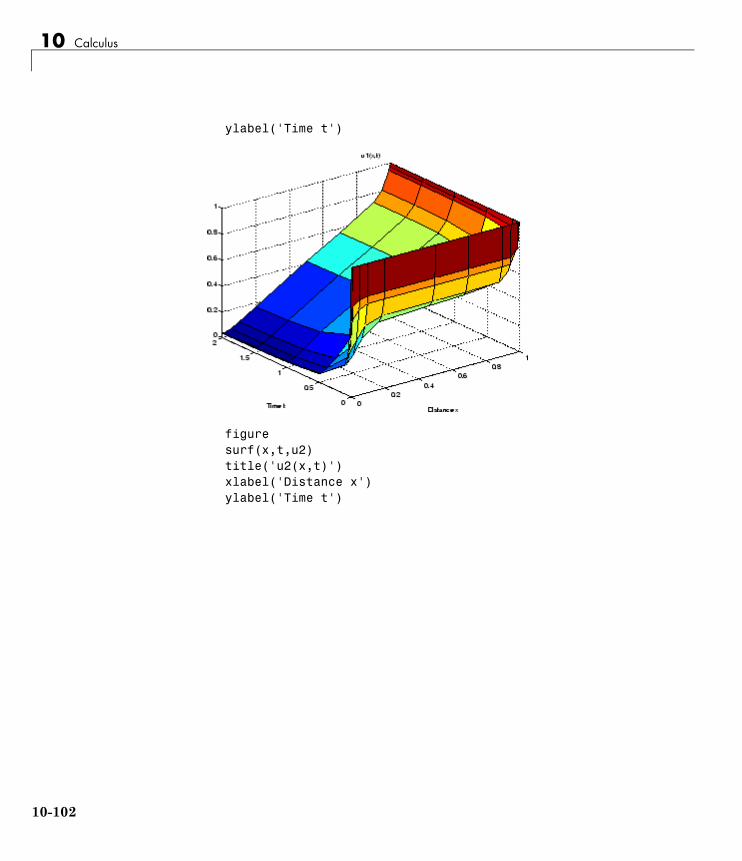
10 Calculus
ylabel('Time t')
figuresurf(x,t,u2)title('u2(x,t)')xlabel('Distance x')ylabel('Time t')
10-102
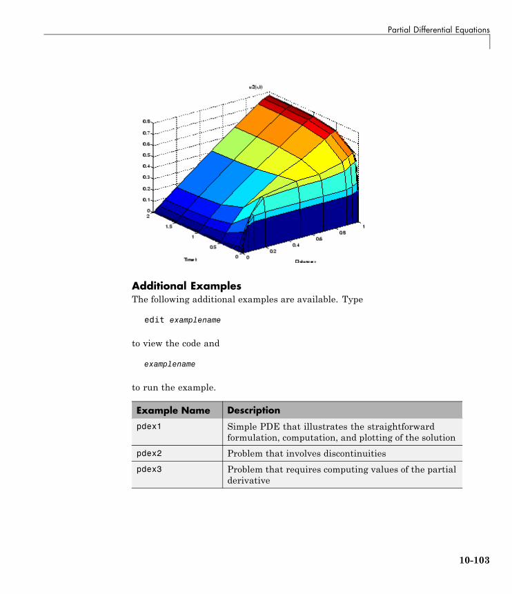
Partial Differential Equations
Additional ExamplesThe following additional examples are available. Type
edit examplename
to view the code and
examplename
to run the example.
Example Name Description
pdex1 Simple PDE that illustrates the straightforwardformulation, computation, and plotting of the solution
pdex2 Problem that involves discontinuities
pdex3 Problem that requires computing values of the partialderivative
10-103
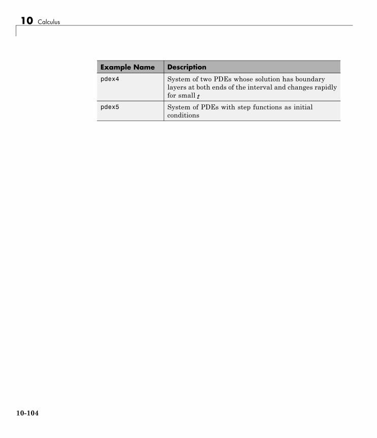
10 Calculus
Example Name Description
pdex4 System of two PDEs whose solution has boundarylayers at both ends of the interval and changes rapidlyfor small
pdex5 System of PDEs with step functions as initialconditions
10-104
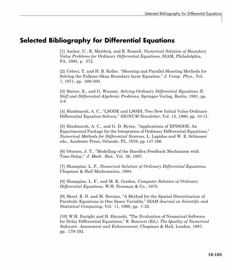
Selected Bibliography for Differential Equations
Selected Bibliography for Differential Equations[1] Ascher, U., R. Mattheij, and R. Russell, Numerical Solution of BoundaryValue Problems for Ordinary Differential Equations, SIAM, Philadelphia,PA, 1995, p. 372.
[2] Cebeci, T. and H. B. Keller, “Shooting and Parallel Shooting Methods forSolving the Falkner-Skan Boundary-layer Equation,” J. Comp. Phys., Vol.7, 1971, pp. 289-300.
[3] Hairer, E., and G. Wanner, Solving Ordinary Differential Equations II,Stiff and Differential-Algebraic Problems, Springer-Verlag, Berlin, 1991, pp.5-8.
[4] Hindmarsh, A. C., “LSODE and LSODI, Two New Initial Value OrdinaryDifferential Equation Solvers,” SIGNUM Newsletter, Vol. 15, 1980, pp. 10-11.
[5] Hindmarsh, A. C., and G. D. Byrne, “Applications of EPISODE: AnExperimental Package for the Integration of Ordinary Differential Equations,”Numerical Methods for Differential Systems, L. Lapidus and W. E. Schiessereds., Academic Press, Orlando, FL, 1976, pp 147-166.
[6] Ottesen, J. T., “Modelling of the Baroflex-Feedback Mechanism withTime-Delay,” J. Math. Biol., Vol. 36, 1997.
[7] Shampine, L. F., Numerical Solution of Ordinary Differential Equations,Chapman & Hall Mathematics, 1994.
[8] Shampine, L. F., and M. K. Gordon, Computer Solution of OrdinaryDifferential Equations, W.H. Freeman & Co., 1975.
[9] Skeel, R. D. and M. Berzins, “A Method for the Spatial Discretization ofParabolic Equations in One Space Variable,” SIAM Journal on Scientific andStatistical Computing, Vol. 11, 1990, pp. 1-32.
[10] W.H. Enright and H. Hayashi, “The Evaluation of Numerical Softwarefor Delay Differential Equations,” R. Boisvert (Ed.), The Quality of NumericalSoftware: Assessment and Enhancement, Chapman & Hall, London, 1997,pp. 179-192.
10-105
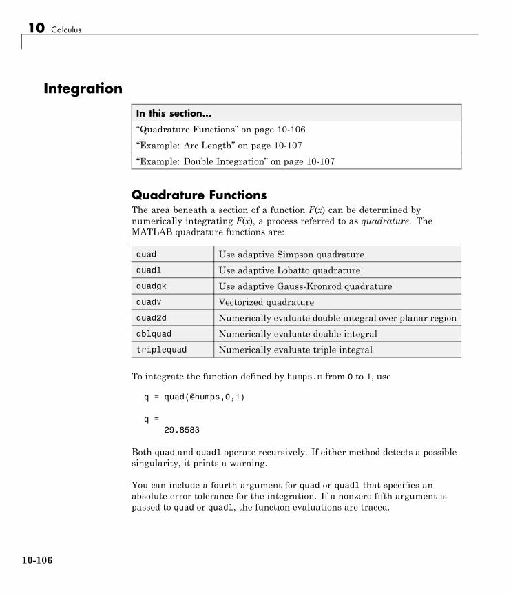
10 Calculus
Integration
In this section...
“Quadrature Functions” on page 10-106
“Example: Arc Length” on page 10-107
“Example: Double Integration” on page 10-107
Quadrature FunctionsThe area beneath a section of a function F(x) can be determined bynumerically integrating F(x), a process referred to as quadrature. TheMATLAB quadrature functions are:
quad Use adaptive Simpson quadrature
quadl Use adaptive Lobatto quadrature
quadgk Use adaptive Gauss-Kronrod quadrature
quadv Vectorized quadrature
quad2d Numerically evaluate double integral over planar region
dblquad Numerically evaluate double integral
triplequad Numerically evaluate triple integral
To integrate the function defined by humps.m from 0 to 1, use
q = quad(@humps,0,1)
q =29.8583
Both quad and quadl operate recursively. If either method detects a possiblesingularity, it prints a warning.
You can include a fourth argument for quad or quadl that specifies anabsolute error tolerance for the integration. If a nonzero fifth argument ispassed to quad or quadl, the function evaluations are traced.
10-106
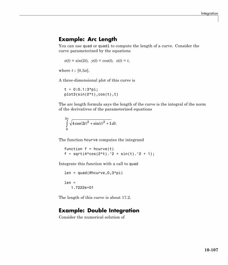
Integration
Example: Arc LengthYou can use quad or quadl to compute the length of a curve. Consider thecurve parameterized by the equations
x(t) = sin(2t), y(t) = cos(t), z(t) = t,
where t [0,3π].
A three-dimensional plot of this curve is
t = 0:0.1:3*pi;plot3(sin(2*t),cos(t),t)
The arc length formula says the length of the curve is the integral of the normof the derivatives of the parameterized equations
4 2 12 2
0
3
cos( ) sin( ) .t t dt+ +∫
The function hcurve computes the integrand
function f = hcurve(t)f = sqrt(4*cos(2*t).^2 + sin(t).^2 + 1);
Integrate this function with a call to quad
len = quad(@hcurve,0,3*pi)
len =1.7222e+01
The length of this curve is about 17.2.
Example: Double IntegrationConsider the numerical solution of
10-107
10 Calculus
f x y dxdyxmin
xmax
ymin
ymax
( , ) .∫∫
For this example f(x,y) = ysin(x) + xcos(y). The first step is to build thefunction to be evaluated. The function must be capable of returning a vectoroutput when given a vector input. You must also consider which variable isin the inner integral, and which goes in the outer integral. In this example,the inner variable is x and the outer variable is y (the order in the integralis dxdy). In this case, the integrand function is
function out = integrnd(x,y)out = y*sin(x) + x*cos(y);
To perform the integration, two functions are available in the funfundirectory. The first, dblquad, is called directly from the command line. Thisfunction evaluates the outer loop using quad. At each iteration, quad calls thesecond helper function that evaluates the inner loop.
To evaluate the double integral, use
result = dblquad(@integrnd,xmin,xmax,ymin,ymax);
The first argument is a string with the name of the integrand function. Thesecond to fifth arguments are
xmin Lower limit of inner integral
xmax Upper limit of the inner integral
ymin Lower limit of outer integral
ymax Upper limit of the outer integral
Here is a numeric example that illustrates the use of dblquad.
xmin = pi;xmax = 2*pi;ymin = 0;ymax = pi;result = dblquad(@integrnd,xmin,xmax,ymin,ymax)
10-108
Integration
The result is -9.8698.
By default, dblquad calls quad. To integrate the previous example usingquadl (with the default values for the tolerance argument), use
result = dblquad(@integrnd,xmin,xmax,ymin,ymax,[],@quadl);
Alternatively, you can pass any user-defined quadrature function name todblquad as long as the quadrature function has the same calling and returnarguments as quad.
10-109

10 Calculus
10-110
11
Fourier Transforms
• “Discrete Fourier Transform (DFT)” on page 11-2
• “Fast Fourier Transform (FFT)” on page 11-8
• “Function Summary” on page 11-28
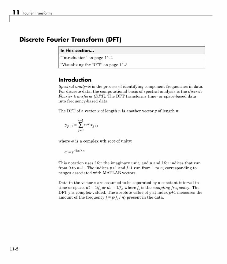
11 Fourier Transforms
Discrete Fourier Transform (DFT)
In this section...
“Introduction” on page 11-2
“Visualizing the DFT” on page 11-3
IntroductionSpectral analysis is the process of identifying component frequencies in data.For discrete data, the computational basis of spectral analysis is the discreteFourier transform (DFT). The DFT transforms time- or space-based datainto frequency-based data.
The DFT of a vector x of length n is another vector y of length n:
y xpjp
jj
n
+ +=
−= ∑1 1
0
1
where ω is a complex nth root of unity:
= −e i n2 /
This notation uses i for the imaginary unit, and p and j for indices that runfrom 0 to n–1. The indices p+1 and j+1 run from 1 to n, corresponding toranges associated with MATLAB vectors.
Data in the vector x are assumed to be separated by a constant interval intime or space, dt = 1/fs or ds = 1/fs, where fs is the sampling frequency. TheDFT y is complex-valued. The absolute value of y at index p+1 measures theamount of the frequency f = p(fs / n) present in the data.
11-2
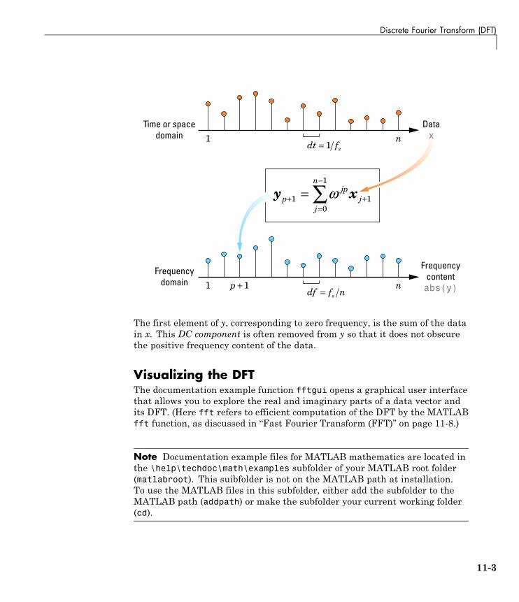
Discrete Fourier Transform (DFT)
Time or spacedomain
pjp
jj
n
s
s
dt fn
pdf f n
+ +=
−
=
=
+=
∑1 10
1
11
Frequencydomain
Frequencycontentabs(y)n1 1
ω
Datax
y x
The first element of y, corresponding to zero frequency, is the sum of the datain x. This DC component is often removed from y so that it does not obscurethe positive frequency content of the data.
Visualizing the DFTThe documentation example function fftgui opens a graphical user interfacethat allows you to explore the real and imaginary parts of a data vector andits DFT. (Here fft refers to efficient computation of the DFT by the MATLABfft function, as discussed in “Fast Fourier Transform (FFT)” on page 11-8.)
Note Documentation example files for MATLAB mathematics are located inthe \help\techdoc\math\examples subfolder of your MATLAB root folder(matlabroot). This suibfolder is not on the MATLAB path at installation.To use the MATLAB files in this subfolder, either add the subfolder to theMATLAB path (addpath) or make the subfolder your current working folder(cd).
11-3

11 Fourier Transforms
If x is a vector,
fftgui(x)
plots the real and imaginary parts of both x and its DFT (fft(x)). Use yourmouse to drag points in any of the plots and the points in the other plotsrespond to the changes.
For example, use fftgui to display the DFT of a unit impulse at x(1):
x = [1 zeros(1,11)];fftgui(x)
11-4
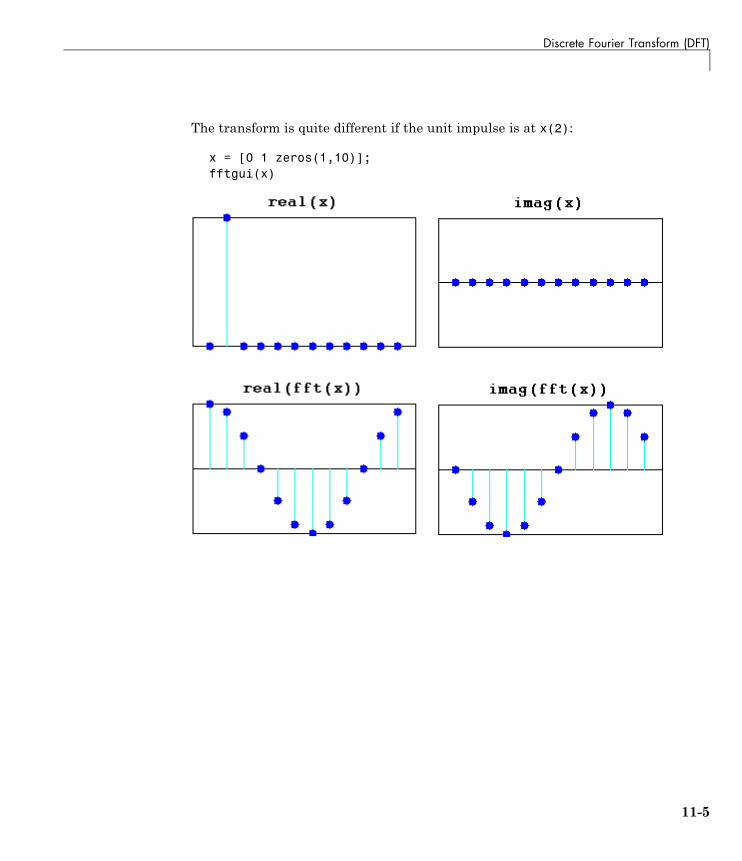
Discrete Fourier Transform (DFT)
The transform is quite different if the unit impulse is at x(2):
x = [0 1 zeros(1,10)];fftgui(x)
11-5
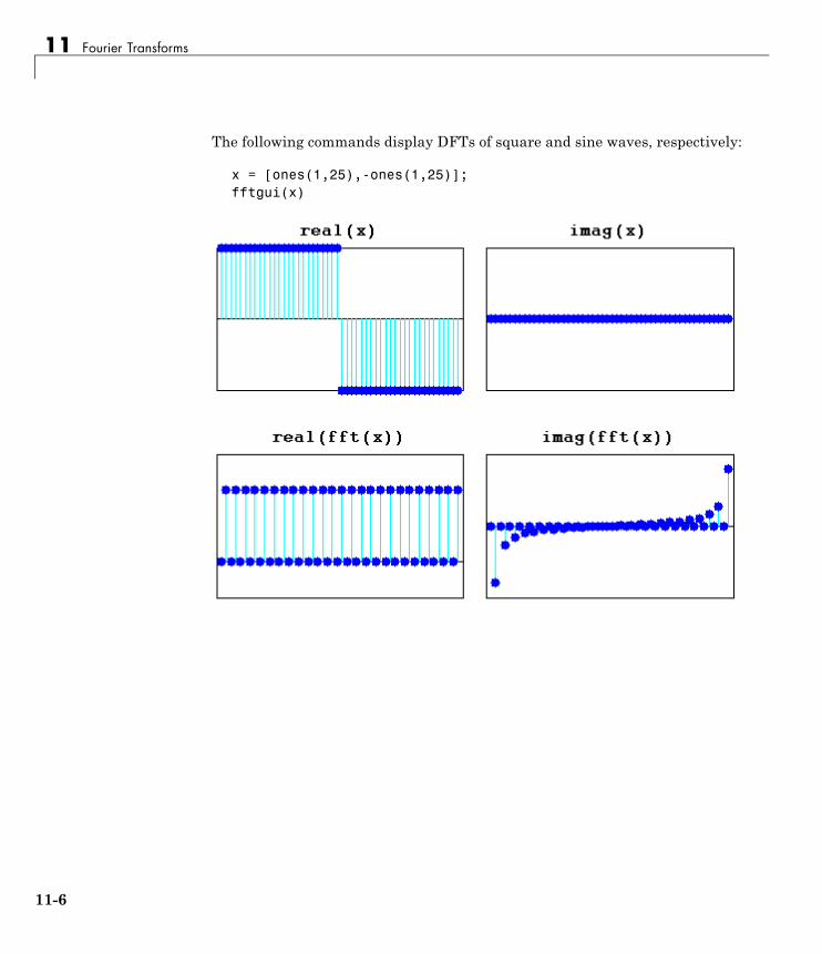
11 Fourier Transforms
The following commands display DFTs of square and sine waves, respectively:
x = [ones(1,25),-ones(1,25)];fftgui(x)
11-6
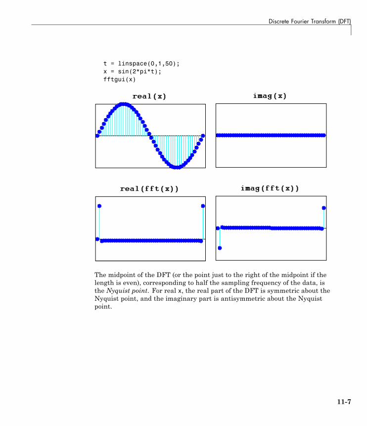
Discrete Fourier Transform (DFT)
t = linspace(0,1,50);x = sin(2*pi*t);fftgui(x)
The midpoint of the DFT (or the point just to the right of the midpoint if thelength is even), corresponding to half the sampling frequency of the data, isthe Nyquist point. For real x, the real part of the DFT is symmetric about theNyquist point, and the imaginary part is antisymmetric about the Nyquistpoint.
11-7
11 Fourier Transforms
Fast Fourier Transform (FFT)
In this section...
“Introduction” on page 11-8
“The FFT in One Dimension” on page 11-9
“The FFT in Multiple Dimensions” on page 11-23
IntroductionDFTs with a million points are common in many applications. Modern signaland image processing applications would be impossible without an efficientmethod for computing the DFT.
Direct application of the definition of the DFT (see “Discrete FourierTransform (DFT)” on page 11-2) to a data vector of length n requires nmultiplications and n additions—a total of 2n2 floating-point operations. Thisdoes not include the generation of the powers of the complex nth root ofunity ω. To compute a million-point DFT, a computer capable of doing onemultiplication and addition every microsecond requires a million seconds, orabout 11.5 days.
Fast Fourier Transform (FFT) algorithms have computational complexity O(nlog n) instead of O(n2). If n is a power of 2, a one-dimensional FFT of length nrequires less than 3n log2 n floating-point operations (times a proportionalityconstant). For n = 220, that is a factor of almost 35,000 faster than 2n2.
The MATLAB functions fft, fft2, and fftn (and their inverses ifft, ifft2,and ifftn, respectively) all use fast Fourier transform algorithms to computethe DFT.
Note MATLAB FFT algorithms are based on FFTW, “The Fastest FourierTransform in the West” (http://www.fftw.org). See fft and fftw for details.
When using FFT algorithms, a distinction is made between the window lengthand the transform length. The window length is the length of the input datavector. It is determined by, for example, the size of an external buffer. The
11-8
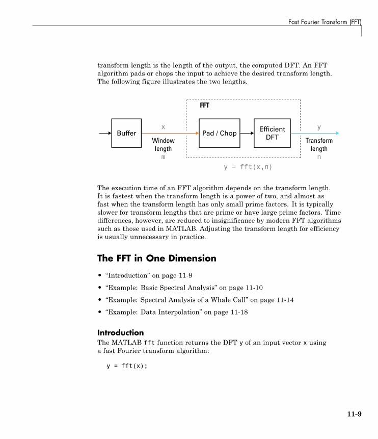
Fast Fourier Transform (FFT)
transform length is the length of the output, the computed DFT. An FFTalgorithm pads or chops the input to achieve the desired transform length.The following figure illustrates the two lengths.
Transformlengthn
Windowlengthm
y = fft(x,n)
yx
FFT
Buffer Pad / ChopEfficient
DFT
The execution time of an FFT algorithm depends on the transform length.It is fastest when the transform length is a power of two, and almost asfast when the transform length has only small prime factors. It is typicallyslower for transform lengths that are prime or have large prime factors. Timedifferences, however, are reduced to insignificance by modern FFT algorithmssuch as those used in MATLAB. Adjusting the transform length for efficiencyis usually unnecessary in practice.
The FFT in One Dimension
• “Introduction” on page 11-9
• “Example: Basic Spectral Analysis” on page 11-10
• “Example: Spectral Analysis of a Whale Call” on page 11-14
• “Example: Data Interpolation” on page 11-18
IntroductionThe MATLAB fft function returns the DFT y of an input vector x usinga fast Fourier transform algorithm:
y = fft(x);
11-9
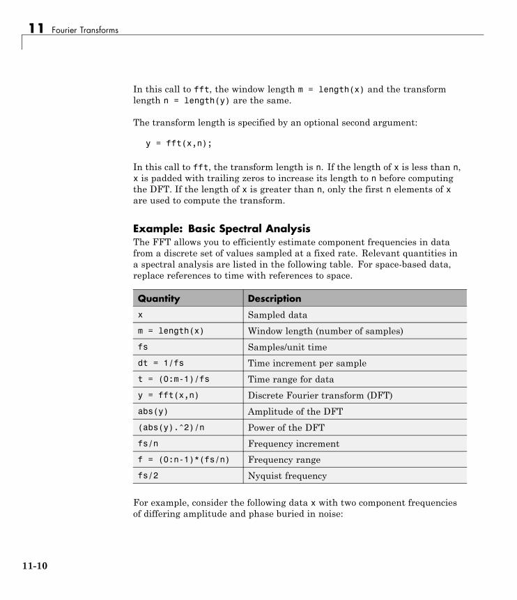
11 Fourier Transforms
In this call to fft, the window length m = length(x) and the transformlength n = length(y) are the same.
The transform length is specified by an optional second argument:
y = fft(x,n);
In this call to fft, the transform length is n. If the length of x is less than n,x is padded with trailing zeros to increase its length to n before computingthe DFT. If the length of x is greater than n, only the first n elements of xare used to compute the transform.
Example: Basic Spectral AnalysisThe FFT allows you to efficiently estimate component frequencies in datafrom a discrete set of values sampled at a fixed rate. Relevant quantities ina spectral analysis are listed in the following table. For space-based data,replace references to time with references to space.
Quantity Description
x Sampled data
m = length(x) Window length (number of samples)
fs Samples/unit time
dt = 1/fs Time increment per sample
t = (0:m-1)/fs Time range for data
y = fft(x,n) Discrete Fourier transform (DFT)
abs(y) Amplitude of the DFT
(abs(y).^2)/n Power of the DFT
fs/n Frequency increment
f = (0:n-1)*(fs/n) Frequency range
fs/2 Nyquist frequency
For example, consider the following data x with two component frequenciesof differing amplitude and phase buried in noise:
11-10
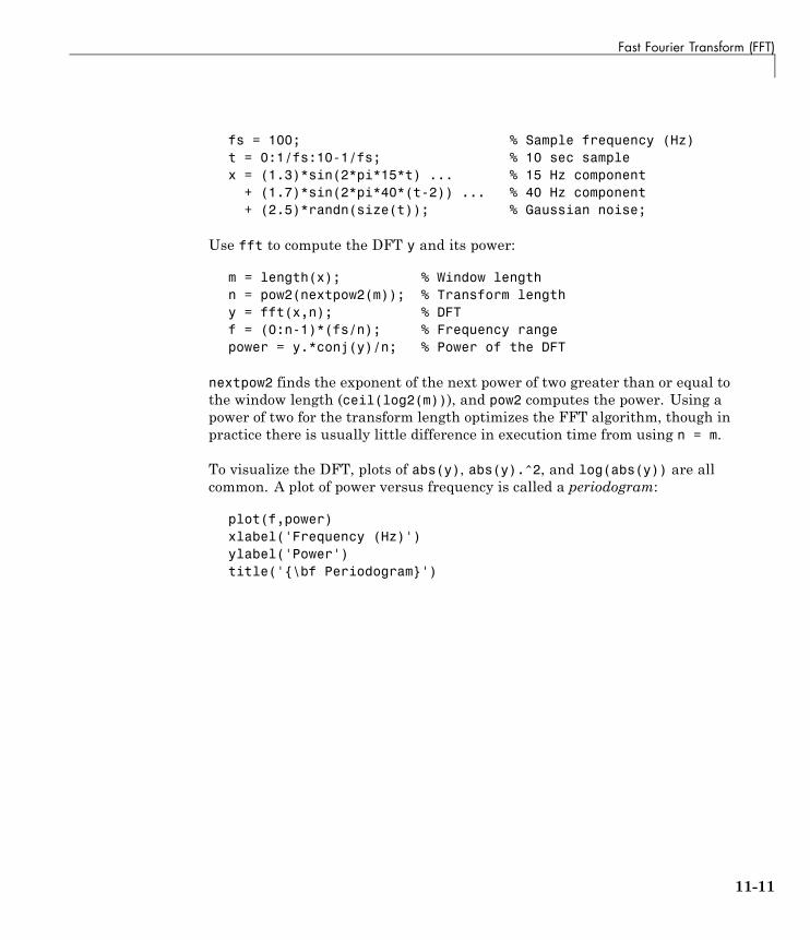
Fast Fourier Transform (FFT)
fs = 100; % Sample frequency (Hz)t = 0:1/fs:10-1/fs; % 10 sec samplex = (1.3)*sin(2*pi*15*t) ... % 15 Hz component
+ (1.7)*sin(2*pi*40*(t-2)) ... % 40 Hz component+ (2.5)*randn(size(t)); % Gaussian noise;
Use fft to compute the DFT y and its power:
m = length(x); % Window lengthn = pow2(nextpow2(m)); % Transform lengthy = fft(x,n); % DFTf = (0:n-1)*(fs/n); % Frequency rangepower = y.*conj(y)/n; % Power of the DFT
nextpow2 finds the exponent of the next power of two greater than or equal tothe window length (ceil(log2(m))), and pow2 computes the power. Using apower of two for the transform length optimizes the FFT algorithm, though inpractice there is usually little difference in execution time from using n = m.
To visualize the DFT, plots of abs(y), abs(y).^2, and log(abs(y)) are allcommon. A plot of power versus frequency is called a periodogram:
plot(f,power)xlabel('Frequency (Hz)')ylabel('Power')title('{\bf Periodogram}')
11-11
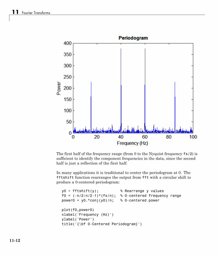
11 Fourier Transforms
The first half of the frequency range (from 0 to the Nyquist frequency fs/2) issufficient to identify the component frequencies in the data, since the secondhalf is just a reflection of the first half.
In many applications it is traditional to center the periodogram at 0. Thefftshift function rearranges the output from fft with a circular shift toproduce a 0-centered periodogram:
y0 = fftshift(y); % Rearrange y valuesf0 = (-n/2:n/2-1)*(fs/n); % 0-centered frequency rangepower0 = y0.*conj(y0)/n; % 0-centered power
plot(f0,power0)xlabel('Frequency (Hz)')ylabel('Power')title('{\bf 0-Centered Periodogram}')
11-12
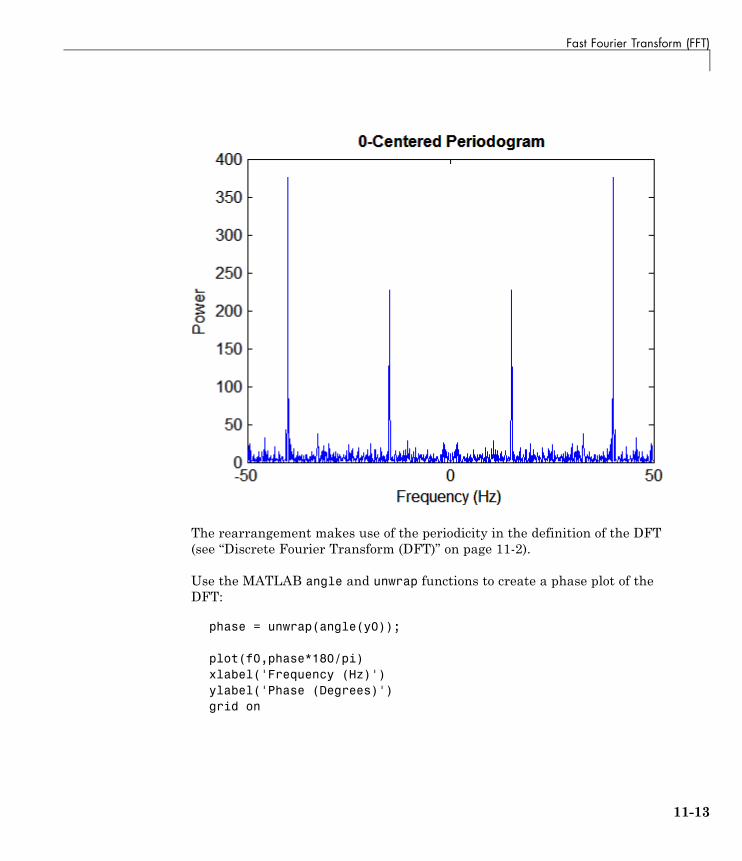
Fast Fourier Transform (FFT)
The rearrangement makes use of the periodicity in the definition of the DFT(see “Discrete Fourier Transform (DFT)” on page 11-2).
Use the MATLAB angle and unwrap functions to create a phase plot of theDFT:
phase = unwrap(angle(y0));
plot(f0,phase*180/pi)xlabel('Frequency (Hz)')ylabel('Phase (Degrees)')grid on
11-13
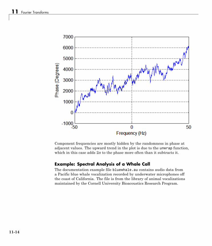
11 Fourier Transforms
Component frequencies are mostly hidden by the randomness in phase atadjacent values. The upward trend in the plot is due to the unwrap function,which in this case adds 2π to the phase more often than it subtracts it.
Example: Spectral Analysis of a Whale CallThe documentation example file bluewhale.au contains audio data froma Pacific blue whale vocalization recorded by underwater microphones offthe coast of California. The file is from the library of animal vocalizationsmaintained by the Cornell University Bioacoustics Research Program.
11-14
Fast Fourier Transform (FFT)
Note Documentation example files for MATLAB mathematics are located inthe \help\techdoc\math\examples subfolder of your MATLAB root folder(matlabroot). This subfolder is not on the MATLAB path at installation.To use the MATLAB files in this subfolder, either add the subfolder to theMATLAB path (addpath) or make the subfolder your current working folder(cd).
Because blue whale calls are so low, they are barely audible to humans. Thetime scale in the data is compressed by a factor of 10 to raise the pitch andmake the call more clearly audible. The following reads, plots, and playsthe data:
[x,fs] = auread('bluewhale.au');
plot(x)xlabel('Sample Number')ylabel('Amplitude')title('{\bf Blue Whale Call}')
sound(x,fs)
11-15
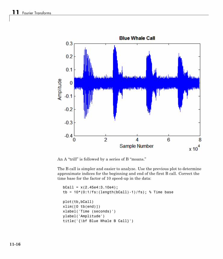
11 Fourier Transforms
An A “trill” is followed by a series of B “moans.”
The B call is simpler and easier to analyze. Use the previous plot to determineapproximate indices for the beginning and end of the first B call. Correct thetime base for the factor of 10 speed-up in the data:
bCall = x(2.45e4:3.10e4);tb = 10*(0:1/fs:(length(bCall)-1)/fs); % Time base
plot(tb,bCall)xlim([0 tb(end)])xlabel('Time (seconds)')ylabel('Amplitude')title('{\bf Blue Whale B Call}')
11-16
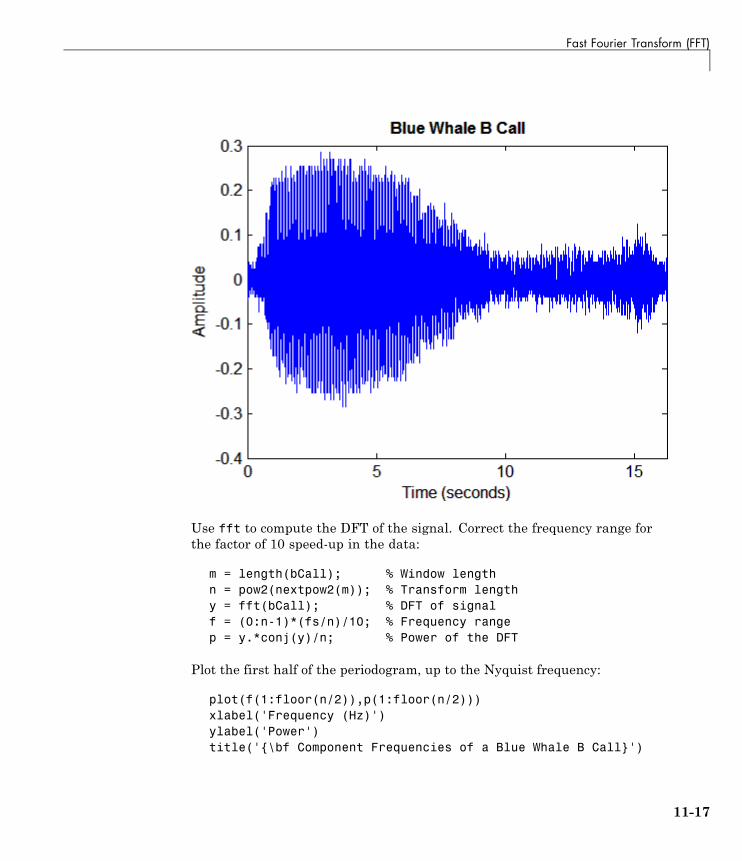
Fast Fourier Transform (FFT)
Use fft to compute the DFT of the signal. Correct the frequency range forthe factor of 10 speed-up in the data:
m = length(bCall); % Window lengthn = pow2(nextpow2(m)); % Transform lengthy = fft(bCall); % DFT of signalf = (0:n-1)*(fs/n)/10; % Frequency rangep = y.*conj(y)/n; % Power of the DFT
Plot the first half of the periodogram, up to the Nyquist frequency:
plot(f(1:floor(n/2)),p(1:floor(n/2)))xlabel('Frequency (Hz)')ylabel('Power')title('{\bf Component Frequencies of a Blue Whale B Call}')
11-17
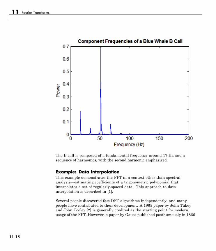
11 Fourier Transforms
The B call is composed of a fundamental frequency around 17 Hz and asequence of harmonics, with the second harmonic emphasized.
Example: Data InterpolationThis example demonstrates the FFT in a context other than spectralanalysis—estimating coefficients of a trigonometric polynomial thatinterpolates a set of regularly-spaced data. This approach to datainterpolation is described in [1].
Several people discovered fast DFT algorithms independently, and manypeople have contributed to their development. A 1965 paper by John Tukeyand John Cooley [2] is generally credited as the starting point for modernusage of the FFT. However, a paper by Gauss published posthumously in 1866
11-18
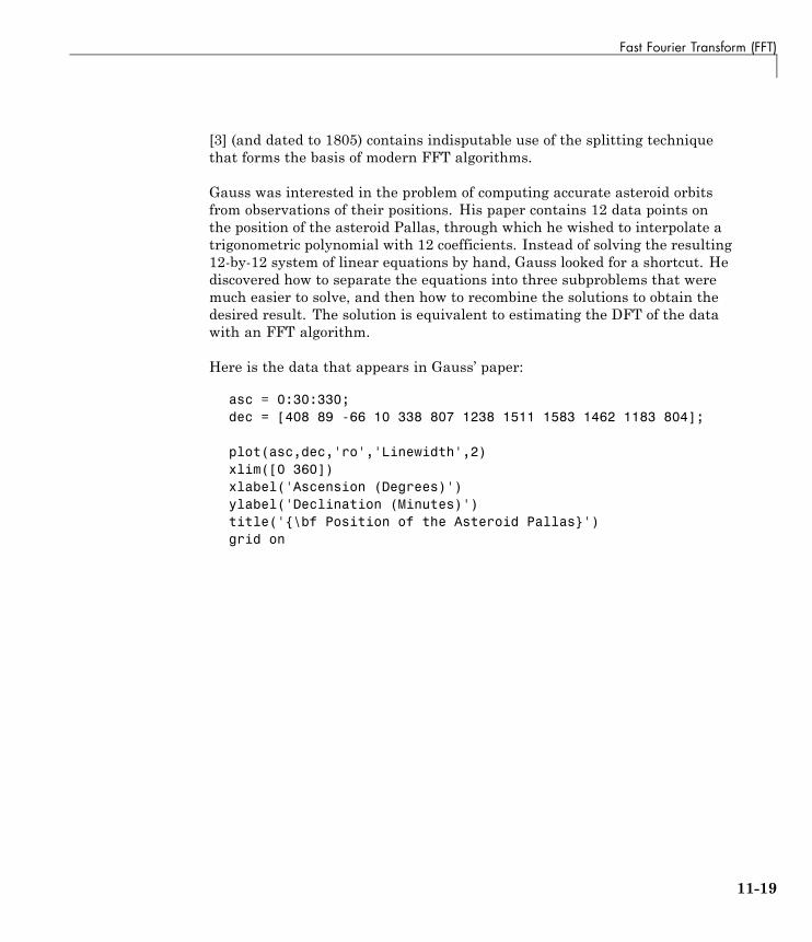
Fast Fourier Transform (FFT)
[3] (and dated to 1805) contains indisputable use of the splitting techniquethat forms the basis of modern FFT algorithms.
Gauss was interested in the problem of computing accurate asteroid orbitsfrom observations of their positions. His paper contains 12 data points onthe position of the asteroid Pallas, through which he wished to interpolate atrigonometric polynomial with 12 coefficients. Instead of solving the resulting12-by-12 system of linear equations by hand, Gauss looked for a shortcut. Hediscovered how to separate the equations into three subproblems that weremuch easier to solve, and then how to recombine the solutions to obtain thedesired result. The solution is equivalent to estimating the DFT of the datawith an FFT algorithm.
Here is the data that appears in Gauss’ paper:
asc = 0:30:330;dec = [408 89 -66 10 338 807 1238 1511 1583 1462 1183 804];
plot(asc,dec,'ro','Linewidth',2)xlim([0 360])xlabel('Ascension (Degrees)')ylabel('Declination (Minutes)')title('{\bf Position of the Asteroid Pallas}')grid on
11-19
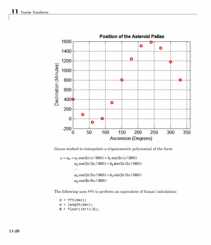
11 Fourier Transforms
Gauss wished to interpolate a trigonometric polynomial of the form:
y a a x b xa x b
= + ++
0 1 1
2 2
2 360 2 3602 2 360
cos( ( / )) sin( ( / ))cos( ( / ))
ssin( ( / ))
cos( ( / )) sin( ( / ))cos(
2 2 360
2 5 360 2 5 3605 5
6
x
a x b xa
�+
22 6 360 ( / ))x
The following uses fft to perform an equivalent of Gauss’ calculation:
d = fft(dec);m = length(dec);M = floor((m+1)/2);
11-20
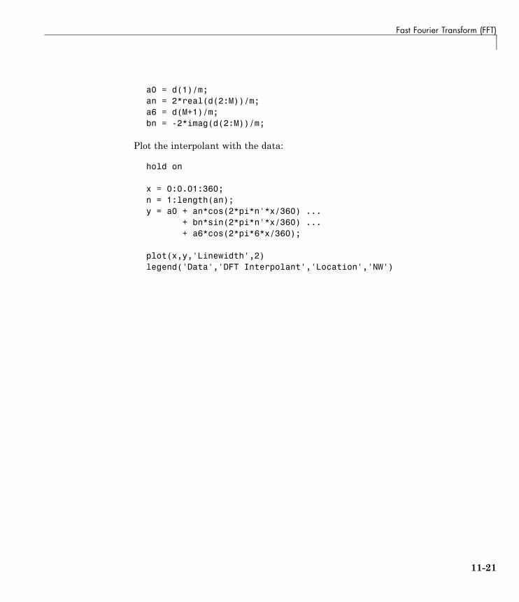
Fast Fourier Transform (FFT)
a0 = d(1)/m;an = 2*real(d(2:M))/m;a6 = d(M+1)/m;bn = -2*imag(d(2:M))/m;
Plot the interpolant with the data:
hold on
x = 0:0.01:360;n = 1:length(an);y = a0 + an*cos(2*pi*n'*x/360) ...
+ bn*sin(2*pi*n'*x/360) ...+ a6*cos(2*pi*6*x/360);
plot(x,y,'Linewidth',2)legend('Data','DFT Interpolant','Location','NW')
11-21
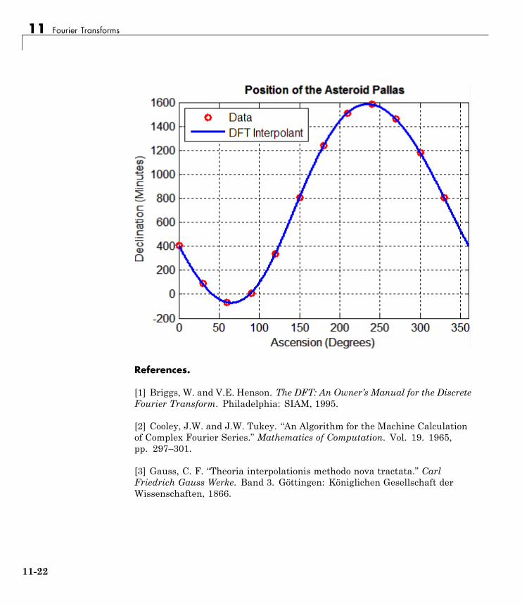
11 Fourier Transforms
References.
[1] Briggs, W. and V.E. Henson. The DFT: An Owner’s Manual for the DiscreteFourier Transform. Philadelphia: SIAM, 1995.
[2] Cooley, J.W. and J.W. Tukey. “An Algorithm for the Machine Calculationof Complex Fourier Series.” Mathematics of Computation. Vol. 19. 1965,pp. 297–301.
[3] Gauss, C. F. “Theoria interpolationis methodo nova tractata.” CarlFriedrich Gauss Werke. Band 3. Göttingen: Königlichen Gesellschaft derWissenschaften, 1866.
11-22
Fast Fourier Transform (FFT)
[4] Heideman M., D. Johnson, and C. Burrus. “Gauss and the History ofthe Fast Fourier Transform.” Arch. Hist. Exact Sciences. Vol. 34. 1985, pp.265–277.
[5] Goldstine, H. H. A History of Numerical Analysis from the 16th throughthe 19th Century. Berlin: Springer-Verlag, 1977.
The FFT in Multiple Dimensions
• “Introduction” on page 11-23
• “Example: Diffraction Patterns” on page 11-24
IntroductionThis section discusses generalizations of the DFT in one dimension (see“Discrete Fourier Transform (DFT)” on page 11-2).
In two dimensions, the DFT of an m-by-n array X is another m-by-n array Y:
Y Xp q mjp
nkq
j kk
n
j
m
+ + + +=
−
=
−= ∑∑1 1 1 1
0
1
0
1
, ,
where ωm and ωn are complex roots of unity:
m
i m
ni n
e
e
=
=
−
−
2
2
/
/
This notation uses i for the imaginary unit, p and j for indices that runfrom 0 to m–1, and q and k for indices that run from 0 to n–1. The indicesp+1 and j+1 run from 1 to m and the indices q+1 and k+1 run from 1 to n,corresponding to ranges associated with MATLAB arrays.
The MATLAB function fft2 computes two-dimensional DFTs usinga fast Fourier transform algorithm. Y = fft2(X) is equivalent toY = fft(fft(X).').', that is, to computing the one-dimensional DFT of
11-23
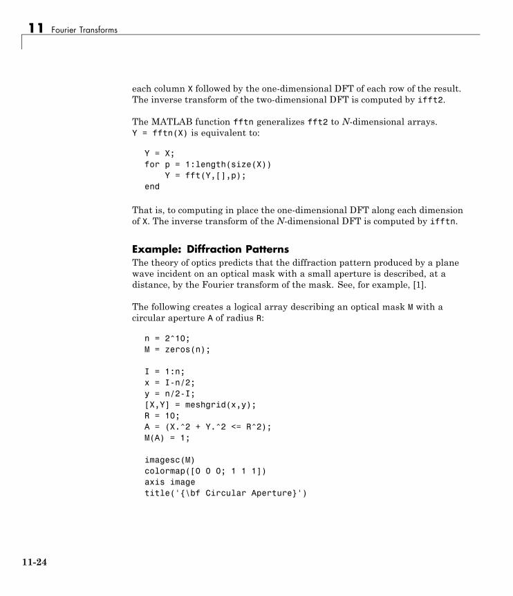
11 Fourier Transforms
each column X followed by the one-dimensional DFT of each row of the result.The inverse transform of the two-dimensional DFT is computed by ifft2.
The MATLAB function fftn generalizes fft2 to N-dimensional arrays.Y = fftn(X) is equivalent to:
Y = X;for p = 1:length(size(X))
Y = fft(Y,[],p);end
That is, to computing in place the one-dimensional DFT along each dimensionof X. The inverse transform of the N-dimensional DFT is computed by ifftn.
Example: Diffraction PatternsThe theory of optics predicts that the diffraction pattern produced by a planewave incident on an optical mask with a small aperture is described, at adistance, by the Fourier transform of the mask. See, for example, [1].
The following creates a logical array describing an optical mask M with acircular aperture A of radius R:
n = 2^10;M = zeros(n);
I = 1:n;x = I-n/2;y = n/2-I;[X,Y] = meshgrid(x,y);R = 10;A = (X.^2 + Y.^2 <= R^2);M(A) = 1;
imagesc(M)colormap([0 0 0; 1 1 1])axis imagetitle('{\bf Circular Aperture}')
11-24
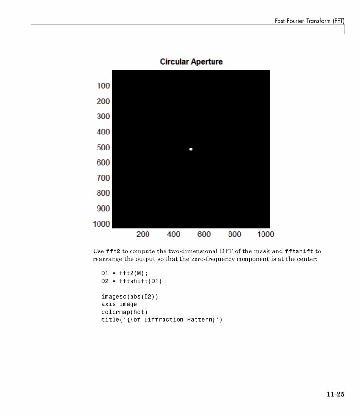
Fast Fourier Transform (FFT)
Use fft2 to compute the two-dimensional DFT of the mask and fftshift torearrange the output so that the zero-frequency component is at the center:
D1 = fft2(M);D2 = fftshift(D1);
imagesc(abs(D2))axis imagecolormap(hot)title('{\bf Diffraction Pattern}')
11-25
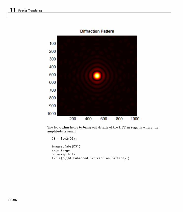
11 Fourier Transforms
The logarithm helps to bring out details of the DFT in regions where theamplitude is small:
D3 = log2(D2);
imagesc(abs(D3))axis imagecolormap(hot)title('{\bf Enhanced Diffraction Pattern}')
11-26
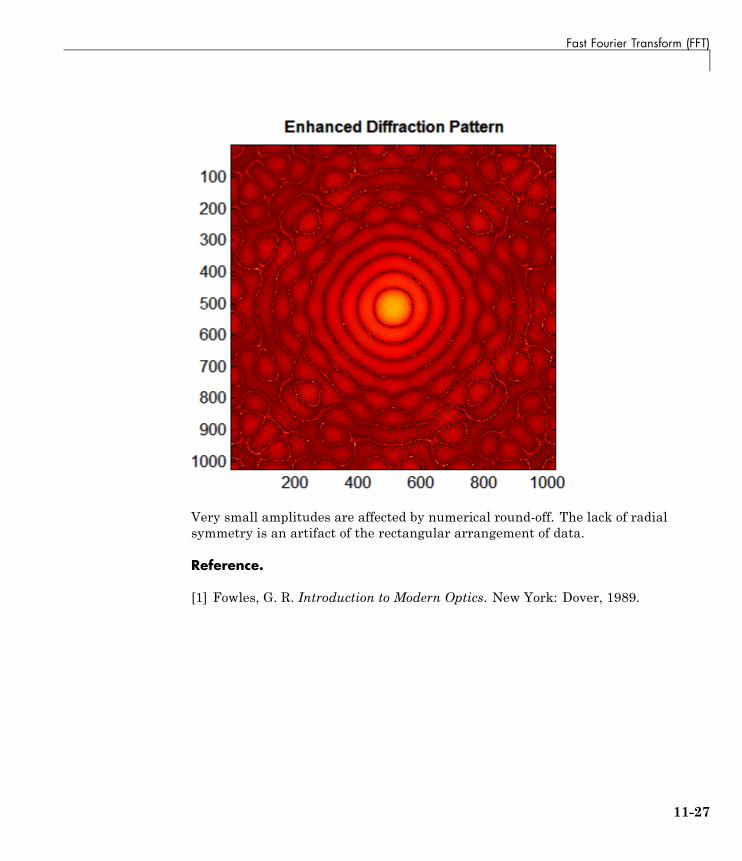
Fast Fourier Transform (FFT)
Very small amplitudes are affected by numerical round-off. The lack of radialsymmetry is an artifact of the rectangular arrangement of data.
Reference.
[1] Fowles, G. R. Introduction to Modern Optics. New York: Dover, 1989.
11-27
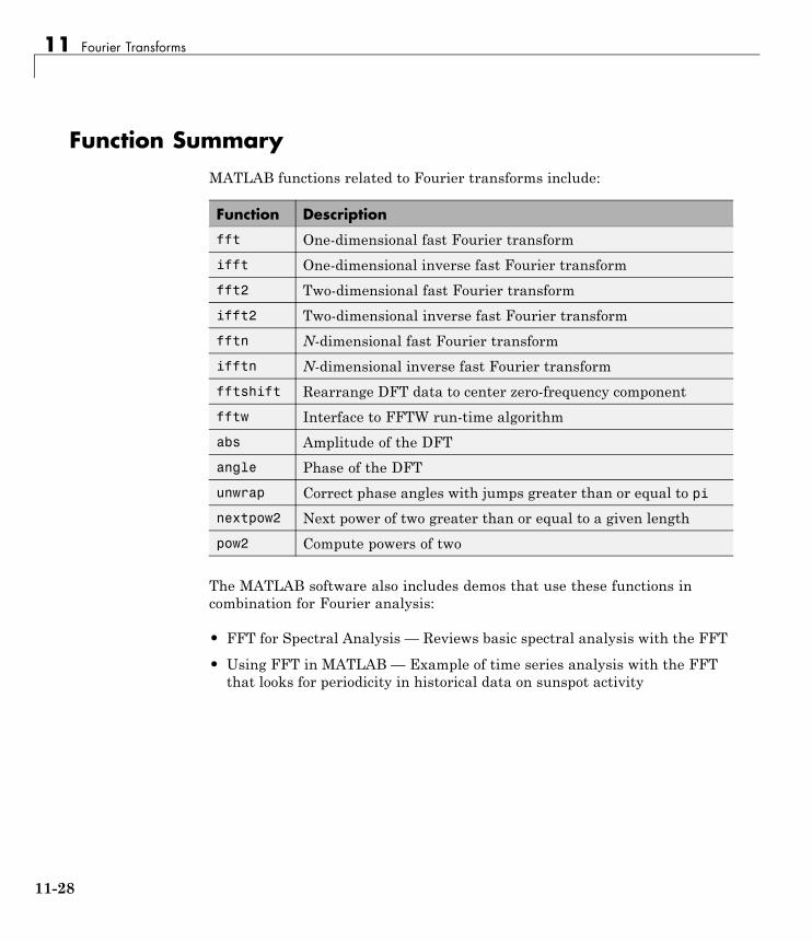
11 Fourier Transforms
Function SummaryMATLAB functions related to Fourier transforms include:
Function Description
fft One-dimensional fast Fourier transform
ifft One-dimensional inverse fast Fourier transform
fft2 Two-dimensional fast Fourier transform
ifft2 Two-dimensional inverse fast Fourier transform
fftn N-dimensional fast Fourier transform
ifftn N-dimensional inverse fast Fourier transform
fftshift Rearrange DFT data to center zero-frequency component
fftw Interface to FFTW run-time algorithm
abs Amplitude of the DFT
angle Phase of the DFT
unwrap Correct phase angles with jumps greater than or equal to pi
nextpow2 Next power of two greater than or equal to a given length
pow2 Compute powers of two
The MATLAB software also includes demos that use these functions incombination for Fourier analysis:
• FFT for Spectral Analysis — Reviews basic spectral analysis with the FFT
• Using FFT in MATLAB — Example of time series analysis with the FFTthat looks for periodicity in historical data on sunspot activity
11-28
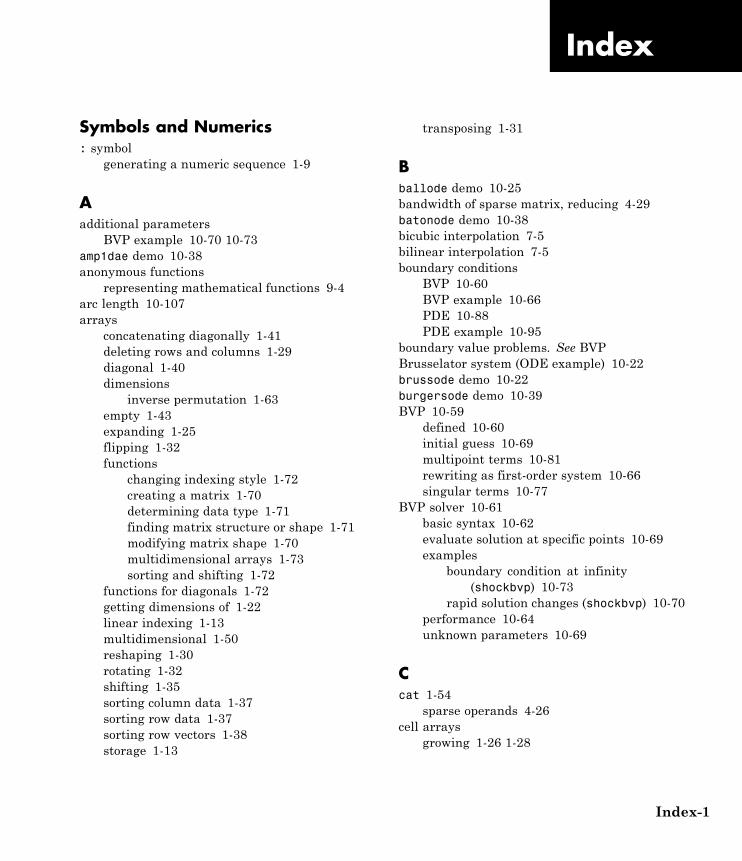
Index
IndexSymbols and Numerics: symbol
generating a numeric sequence 1-9
Aadditional parameters
BVP example 10-70 10-73amp1dae demo 10-38anonymous functions
representing mathematical functions 9-4arc length 10-107arrays
concatenating diagonally 1-41deleting rows and columns 1-29diagonal 1-40dimensions
inverse permutation 1-63empty 1-43expanding 1-25flipping 1-32functions
changing indexing style 1-72creating a matrix 1-70determining data type 1-71finding matrix structure or shape 1-71modifying matrix shape 1-70multidimensional arrays 1-73sorting and shifting 1-72
functions for diagonals 1-72getting dimensions of 1-22linear indexing 1-13multidimensional 1-50reshaping 1-30rotating 1-32shifting 1-35sorting column data 1-37sorting row data 1-37sorting row vectors 1-38storage 1-13
transposing 1-31
Bballode demo 10-25bandwidth of sparse matrix, reducing 4-29batonode demo 10-38bicubic interpolation 7-5bilinear interpolation 7-5boundary conditions
BVP 10-60BVP example 10-66PDE 10-88PDE example 10-95
boundary value problems. See BVPBrusselator system (ODE example) 10-22brussode demo 10-22burgersode demo 10-39BVP 10-59
defined 10-60initial guess 10-69multipoint terms 10-81rewriting as first-order system 10-66singular terms 10-77
BVP solver 10-61basic syntax 10-62evaluate solution at specific points 10-69examples
boundary condition at infinity(shockbvp) 10-73
rapid solution changes (shockbvp) 10-70performance 10-64unknown parameters 10-69
Ccat 1-54
sparse operands 4-26cell arrays
growing 1-26 1-28
Index-1
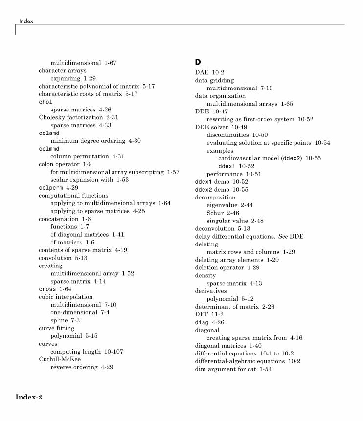
Index
multidimensional 1-67character arrays
expanding 1-29characteristic polynomial of matrix 5-17characteristic roots of matrix 5-17chol
sparse matrices 4-26Cholesky factorization 2-31
sparse matrices 4-33colamd
minimum degree ordering 4-30colmmd
column permutation 4-31colon operator 1-9
for multidimensional array subscripting 1-57scalar expansion with 1-53
colperm 4-29computational functions
applying to multidimensional arrays 1-64applying to sparse matrices 4-25
concatenation 1-6functions 1-7of diagonal matrices 1-41of matrices 1-6
contents of sparse matrix 4-19convolution 5-13creating
multidimensional array 1-52sparse matrix 4-14
cross 1-64cubic interpolation
multidimensional 7-10one-dimensional 7-4spline 7-3
curve fittingpolynomial 5-15
curvescomputing length 10-107
Cuthill-McKeereverse ordering 4-29
DDAE 10-2data gridding
multidimensional 7-10data organization
multidimensional arrays 1-65DDE 10-47
rewriting as first-order system 10-52DDE solver 10-49
discontinuities 10-50evaluating solution at specific points 10-54examples
cardiovascular model (ddex2) 10-55ddex1 10-52
performance 10-51ddex1 demo 10-52ddex2 demo 10-55decomposition
eigenvalue 2-44Schur 2-46singular value 2-48
deconvolution 5-13delay differential equations. See DDEdeleting
matrix rows and columns 1-29deleting array elements 1-29deletion operator 1-29density
sparse matrix 4-13derivatives
polynomial 5-12determinant of matrix 2-26DFT 11-2diag 4-26diagonal
creating sparse matrix from 4-16diagonal matrices 1-40differential equations 10-1 to 10-2differential-algebraic equations 10-2dim argument for cat 1-54
Index-2

Index
dimensionspermuting 1-62removing singleton 1-61
direct methodssystems of sparse equations 4-37
discontinuitiesDDE solver 10-50
discrete Fourier transform (DFT) 11-2displaying
sparse matrices 4-24dot product 2-9
Eeig 1-65eigenvalues 2-44
of sparse matrix 4-40eigenvectors 2-44electrical circuits
DAE example 10-38Emden’s equation
example 10-78empty matrices 1-43end 1-16error tolerance
effects of too large (ODE) 10-45machine precision 10-42
event location (ODE)advanced example 10-28simple example 10-25
expandingcharacter arrays 1-29
expanding cell arrays 1-26 1-28expanding structure arrays 1-26 1-28eye
derivation of the name 2-11sparse matrices 4-26
Ffactorization 4-30
Cholesky 2-31Hermitian positive definite 2-32incomplete 4-35LU 2-33partial pivoting 2-33positive definite 2-31QR 2-34sparse matrices 4-30
Cholesky 4-33LU 4-30triangular 4-30
fast Fourier transform (FFT) 11-8fem1ode demo 10-19fem2ode demo 10-39FFT 11-8
DC component 11-3history 11-18transform length 11-8window length 11-8
find functionsparse matrices 4-21
finite element discretization (ODEexample) 10-19
first-order differential equationsrepresentation for BVP solver 10-66representation for DDE solver 10-52
flipping matrices 1-32Fourier transforms
FFT-based interpolation 7-4fsbvp demo 10-73full 4-26 4-29function functions 9-1functional operators 9-1functions
applyingto multidimensional structure
arrays 1-69changing indexing style 1-72
Index-3
Index
creating a matrix 1-70creating arrays with 1-54creating matrices 1-4determining data type 1-71finding matrix structure or shape 1-71for diagonal matrices 1-72mathematical. See mathematical functionsmatrix concatenation 1-7modifying matrix shape 1-70multidimensional arrays 1-73optimizing 8-1sorting and shifting 1-72sparse matrix 1-48
GGaussian elimination 2-33global minimum 8-27growing an array 1-25growing cell array 1-26 1-28growing structure arrays 1-26 1-28
Hhb1dae demo 10-31hb1ode demo 10-39Hermitian positive definite matrix 2-32higher-order ODEs
rewriting as first-order ODEs 10-5
Iiburgersode demo 10-39identity matrix 2-11ihb1dae demo 10-39importing
sparse matrix 4-18incomplete factorization 4-35indexing
multidimensional arrays 1-56
indices, how MATLAB calculates 1-59infeasible optimization problems 8-27initial conditions
ODE 10-5ODE example 10-11PDE 10-88PDE example 10-94
initial guess (BVP)example 10-67
initial value problemsdefined 10-5
inner product 2-7integration 10-106
double 10-107numerical 10-106triple 10-106See also differential equations
integration intervalPDE (MATLAB) 10-91
interpolationcomparing methods graphically 7-6FFT-based 7-4multidimensional 7-9one-dimensional 7-3speed, memory, smoothness 7-4three-dimensional 7-8two-dimensional 7-5using FFT 11-18
inverse of matrix 2-26inverse permutation of array dimensions 1-63ipermute 1-63iterative methods
sparse matrices 4-38sparse systems of equations 4-37
KKronecker tensor matrix product 2-12
Index-4
Index
Lleast squares 4-35length of curve, computing 10-107linear equations
minimal norm solution 2-28overdetermined systems 2-21rectangular systems 2-27
linear interpolationmultidimensional 7-10one-dimensional 7-3
linear systems of equationsdirect methods (sparse) 4-37full 2-15iterative methods (sparse) 4-37sparse 4-37
linear transformation 2-5load
sparse matrices 4-18Lobatto IIIa BVP solver 10-62LU factorization 2-33
sparse matrices and reordering 4-30
Mmat4bvp demo 10-86mathematical functions
as function input arguments 9-1finding roots 5-6minimizing 8-3numerical integration 10-106
mathematical operationssparse matrices 4-25
Mathieu’s equation (BVP example) 10-65matrices 2-5
accessing multiple elements 1-14accessing single elements 1-12as linear transformation 2-5characteristic polynomial 5-17characteristic roots 5-17concatenating 1-6
concatenating diagonally 1-41constructing a matrix operations
constructing 1-3creating 1-2creation 2-5data structure query 1-24data type query 1-23deleting rows and columns 1-29determinant 2-26diagonal 1-40empty 1-43expanding 1-25flipping 1-32full to sparse conversion 4-13functions
changing indexing style 1-72creating a matrix 1-70determining data type 1-71finding matrix structure or shape 1-71modifying matrix shape 1-70sorting and shifting 1-72
functions for creating 1-4functions for diagonals 1-72getting dimensions of 1-22identity 2-11inverse 2-26iterative methods (sparse) 4-38linear indexing 1-13orthogonal 2-34pseudoinverse 2-27rank deficiency 2-23reshaping 1-30rotating 1-32scalar 1-45shifting 1-35sorting column data 1-37sorting row data 1-37sorting row vectors 1-38symmetric 2-8transposing 1-31
Index-5
Index
triangular 2-31vectors 1-46
matrix operationsaddition and subtraction 2-7concatenating matrices 1-6creating matrices 1-2division 2-16exponentials 2-41multiplication 2-9powers 2-40transpose 2-8
matrix productsKronecker tensor 2-12
max 4-26Maximization 8-7mean 1-64minimizing mathematical functions
of one variable 8-3of several variables 8-5options 8-12
minimum degree ordering 4-29Moore-Penrose pseudoinverse 2-27multidimensional
data gridding 7-10interpolation 7-9
multidimensional arraysapplying functions 1-64
element-by-element functions 1-64matrix functions 1-64vector functions 1-64
cell arrays 1-67computations on 1-64creating 1-52
at the command line 1-52with functions 1-54with the cat function 1-54
extending 1-53format 1-56indexing 1-56
avoiding ambiguity 1-60
with the colon operator 1-57number of dimensions 1-56organizing data 1-65permuting dimensions 1-62removing singleton dimensions 1-61reshaping 1-60size of 1-56storage 1-56structure arrays 1-68
applying functions 1-69subscripts 1-51
multistep solver (ODE) 10-6
Nndgrid 1-73ndims 1-56nearest neighbor interpolation
multidimensional 7-10one-dimensional 7-3three-dimensional 7-9two-dimensional 7-5
nnz 4-19nonstiff ODE examples
rigid body (rigidode) 10-16nonzero elements
maximum number in sparse matrix 4-15number in sparse matrix 4-19sparse matrix 4-19values for sparse matrices 4-19
nonzeros 4-19norms
vector and matrix 2-13numerical integration 10-106
computing length of curve 10-107double 10-107triple 10-106
Nyquist point 11-7nzmax 4-19 4-21
Index-6
Index
Oobjective function
return values 8-27ODE 10-2
coding in MATLAB 10-11first order 10-4overspecified systems 10-40
ODE solver propertiesfixed step sizes 10-41
ODE solversalgorithms
Adams-Bashworth-Moulton PECE 10-6Bogacki-Shampine 10-6Dormand-Prince 10-6modified Rosenbrock formula 10-7numerical differentiation formulas 10-7
backwards in time 10-44basic example
stiff problem 10-13basic syntax 10-8calling 10-11evaluate solution at specific points 10-16examples 10-10minimizing output storage 10-41minimizing startup cost 10-41multistep solver 10-6nonstiff problem example 10-11nonstiff problems 10-6one-step solver 10-6performance 10-9problem size 10-40sampled data 10-44stiff problems 10-7 10-13troubleshooting 10-39
offsets for indexing 1-59one-dimensional interpolation 7-3one-step solver (ODE) 10-6ones
sparse matrices 4-26operators
deletion 1-29optimization 8-1
helpful hints 8-27options parameters 8-12troubleshooting 8-27See also minimizing mathematical functions
orbitode demo 10-28organizing data
multidimensional arrays 1-65orthogonal matrix 2-34outer product 2-7output functions 8-16overdetermined
rectangular matrices 2-21overspecified ODE systems 10-40
Ppage subscripts 1-51partial differential equations. See PDEpartial fraction expansion 5-14PDE 10-87
defined 10-88discretized 10-43
PDE solver (MATLAB) 10-89basic syntax 10-89performance 10-92properties 10-92
pdex2 demo 10-103pdex3 demo 10-103pdex5 demo 10-104performance
de-emphasizing an ODE solutioncomponent 10-42
improving for BVP solver 10-64improving for DDE solver 10-51improving for ODE solvers 10-9improving for PDE solver 10-92
periodogram 11-110-centered 11-12
Index-7
Index
permutations 4-26permute 1-62permuting array dimensions 1-62
inverse 1-63polynomial interpolation 7-3polynomials
calculating coefficients from roots 5-5calculating roots 5-5curve fitting 5-15derivatives 5-12evaluating 5-4multiplying and dividing 5-13partial fraction expansion 5-14representing as vectors 5-3
preconditionersparse matrices 4-35
pseudoinverseof matrix 2-27
pseudorandom 3-1
QQR factorization 2-34 4-34quad, quadl functions
differ from ODE solvers 10-40quadrature. See numerical integration
Rrand
sparse matrices 4-26randn 1-54random number generators 3-1rank deficiency
detecting 2-36rectangular matrices 2-23sparse matrices 4-35
rectangular matricesidentity 2-11overdetermined systems 2-21
pseudoinverse 2-27QR factorization 2-34rank deficient 2-23singular value decomposition 2-48
removingsingleton dimensions 1-61
reorderings 4-26for sparser factorizations 4-29LU factorization 4-30minimum degree ordering 4-29reducing bandwidth 4-29
repmap 1-54reshape 1-60reshaping
multidimensional arrays 1-60reshaping matrices 1-30rigid body (ODE example) 10-16rigidode demo 10-16Robertson problem
DAE example 10-31ODE example 10-39
rootsof mathematical functions 5-6polynomial 5-5
rotating matrices 1-32
Ssampled data
with ODE solvers 10-44sampling frequency 11-2save 4-18scalar
as a matrix 2-6scalar product 2-9scalars 1-45Schur decomposition 2-46second difference operator 4-15shiftdim 1-73shifting matrix elements 1-35
Index-8
Index
shockbvp demo 10-70sin 1-64singular value matrix decomposition 2-48size
sparse matrices 4-25solution changes, rapid
making initial guess 10-70verifying consistent behavior 10-73
solving linear systems of equationsfull 2-15sparse 4-37
sort 4-29sorting matrix column data 1-37sorting matrix row data 1-37sorting matrix row vectors 1-38sparse function
converting full to sparse 4-13sparse matrix
advantages 4-11Cholesky factorization 4-33computational considerations 4-25contents 4-19conversion from full 4-13creating 4-13
directly 4-14from diagonal elements 4-16
density 4-13eigenvalues 4-40importing 4-18linear systems of equations 4-37LU factorization 4-30
and reordering 4-30mathematical operations 4-25nonzero elements 4-19
maximum number 4-15specifying when creating matrix 4-14storage 4-19values 4-19
nonzero elements of sparse matrixnumber of 4-19
operations 4-25permutation 4-26preconditioner 4-35propagation through computations 4-25QR factorization 4-34reordering 4-26storage 4-10
for various permutations 4-28viewing 4-19
triangular factorization 4-30viewing contents graphically 4-24viewing storage 4-19
sparse matrix functions 1-48sparse ODE examples
Brusselator system (brussode) 10-22spconvert 4-18spdiags 4-16spectral analysis 11-2
audio data 11-14basic example 11-10
speye 4-26spones 4-29spparms 4-38sprand 4-26spy 4-24squeeze 1-61
with multidimensional arguments 1-65startup cost
minimizing for ODE solvers 10-41stiff ODE examples
Brusselator system (brussode) 10-22differential-algebraic problem
(hb1dae) 10-31finite element discretization (fem1ode) 10-19
stiffness (ODE), defined 10-13storage
minimizing for ODE problems 10-41permutations of sparse matrices 4-28sparse matrix 4-10viewing for sparse matrix 4-19
Index-9
Index
structure arraysgrowing 1-26 1-28multidimensional 1-68
applying functions 1-69subscripting
how MATLAB calculates indices 1-59multidimensional arrays 1-51page 1-51
sum 1-64counting nonzeros in sparse matrix 4-29sparse matrices 4-26
symamdminimum degree ordering 4-30
symmetric matrixtranspose 2-8
symrcmcolumn permutation 4-31reducing sparse matrix bandwidth 4-29
systems of equations.. See linear systems ofequations
Tthree-dimensional interpolation 7-8threebvp demo 10-86transfer functions
using partial fraction expansion 5-14transpose 1-63
complex conjugate 2-9unconjugated complex 2-9
transposing matrices 1-31triangular factorization
sparse matrices 4-30triangular matrix 2-31tricubic interpolation 7-9trigonometric functions 1-64trilinear interpolation 7-9
troubleshooting (ODE) 10-39two-dimensional interpolation 7-5
comparing methods graphically 7-6twobvp demo 10-86
Uunitary matrices
QR factorization 2-34unknown parameters (BVP) 10-69
Vvan der Pol example
simple, nonstiff 10-11simple, stiff 10-13
vector productsdot or scalar 2-9outer and inner 2-7
vectors 1-46column and row 2-6multiplication 2-7
visualizing solver resultsBVP 10-68DDE 10-53ODE 10-12PDE 10-96
Wwhos 1-56
Zzeros 1-54
sparse matrices 4-26
Index-10


