Ralph C. Smith Department of Mathematics North Carolina State University Introduction to MATLAB and Linear Algebra Overview: 1. MATLAB examples throughout tutorial 2. Elements of linear algebra • Fundamental properties of vectors and matrices • Eigenvalues, eigenvectors and singular values Linear Algebra and Numerical Matrix Theory: • Vector properties including orthogonality • Matrix analysis, inversion and solving Ax = b for very large systems • Eigen- and singular value decompositions
Transcript
Ralph C. SmithDepartment of Mathematics
North Carolina State University
Introduction to MATLAB and Linear Algebra
Overview: 1. MATLAB examples throughout tutorial
2. Elements of linear algebra
• Fundamental properties of vectors and matrices
• Eigenvalues, eigenvectors and singular values
Linear Algebra and Numerical Matrix Theory:
• Vector properties including orthogonality
• Matrix analysis, inversion and solving Ax = b for very large systems
• Eigen- and singular value decompositions
Linear Algebra and Numerical Matrix Theory
Topics: Illustrate with MATLAB as topics are introduced
• Basic concepts
• Linear transformations
• Linear independence, basis vectors, and span of a vector space
• Fundamental Theorem of Linear Algebra
• Determinants and matrix rank
• Eigenvalues and eigenvectors
• Solving Ax = b and condition numbers
• Singular value decomposition (SVD)
• Cholesky and QR decompositions
Linear Algebra has become as basic and as applicable as calculus, and fortunately it is easier.
--Gilbert Strang, MIT
Vectors and Matrices
• Vector in Rn is an ordered set of n real numbers.– e.g. v = (1,6,3,4) is in R4
– “(1,6,3,4)” is a column vector:
– as opposed to a row vector:
• m-by-n matrix is an object with m rows and n columns, each entry fill with a real number:
÷÷÷÷÷
ø
ö
ççççç
è
æ
4361
( )4361
÷÷÷
ø
ö
ççç
è
æ
2396784821
Note:
Vector Norms
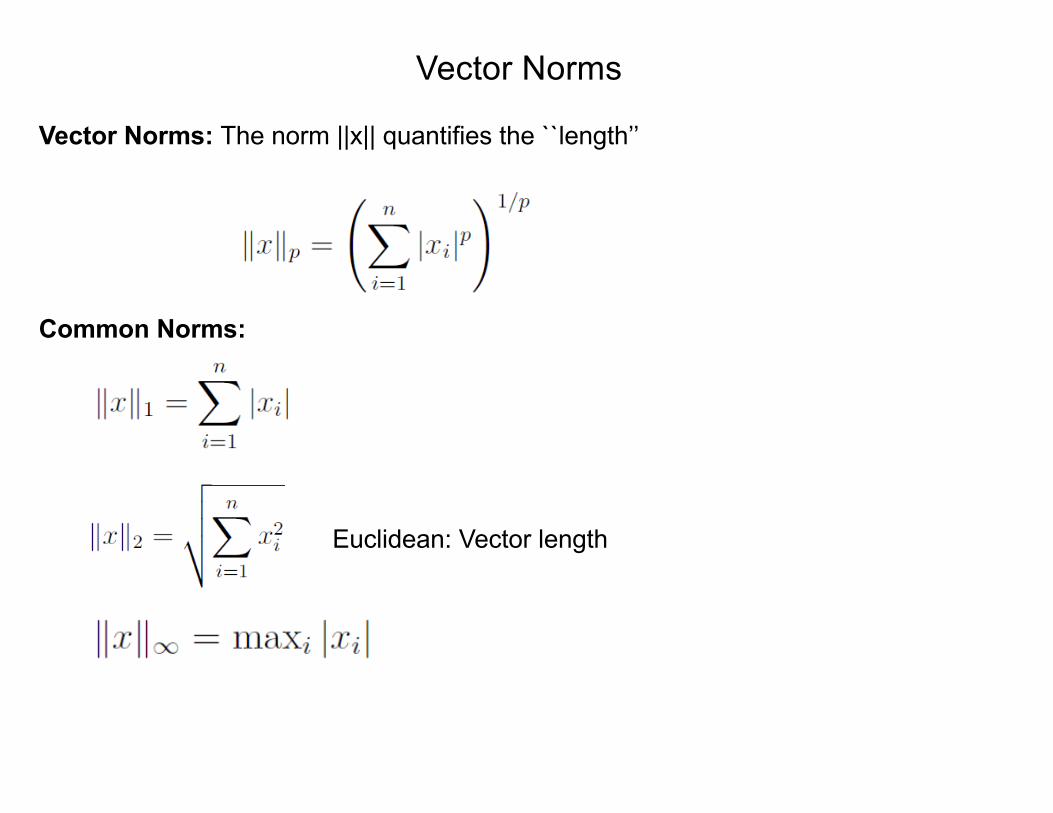
Vector Norms: The norm ||x|| quantifies the ``length’’
Common Norms:
Euclidean: Vector length
Vector and Matrix Products
Vector products:– Dot product: ( ) 2211
2
121 vuvuvv
uuvuvu T +=÷÷ø
öççè
æ==•
( ) ÷÷ø
öççè
æ=÷÷
ø
öççè
æ=
2212
211121
2
1
vuvuvuvu
vvuu
uvT
Matrix Product:
÷÷ø
öççè
æ++++
=
÷÷ø
öççè
æ=÷÷
ø
öççè
æ=
2222122121221121
2212121121121111
2221
1211
2221
1211 ,
babababababababa
AB
bbbb
Baaaa
A
– Outer product:
Note: )cos(qBABA =×
If u•v=0, ||u||2 != 0, ||v||2 != 0 à u and v are orthogonal
If u•v=0, ||u||2 = 1, ||v||2 = 1 à u and v are orthonormal
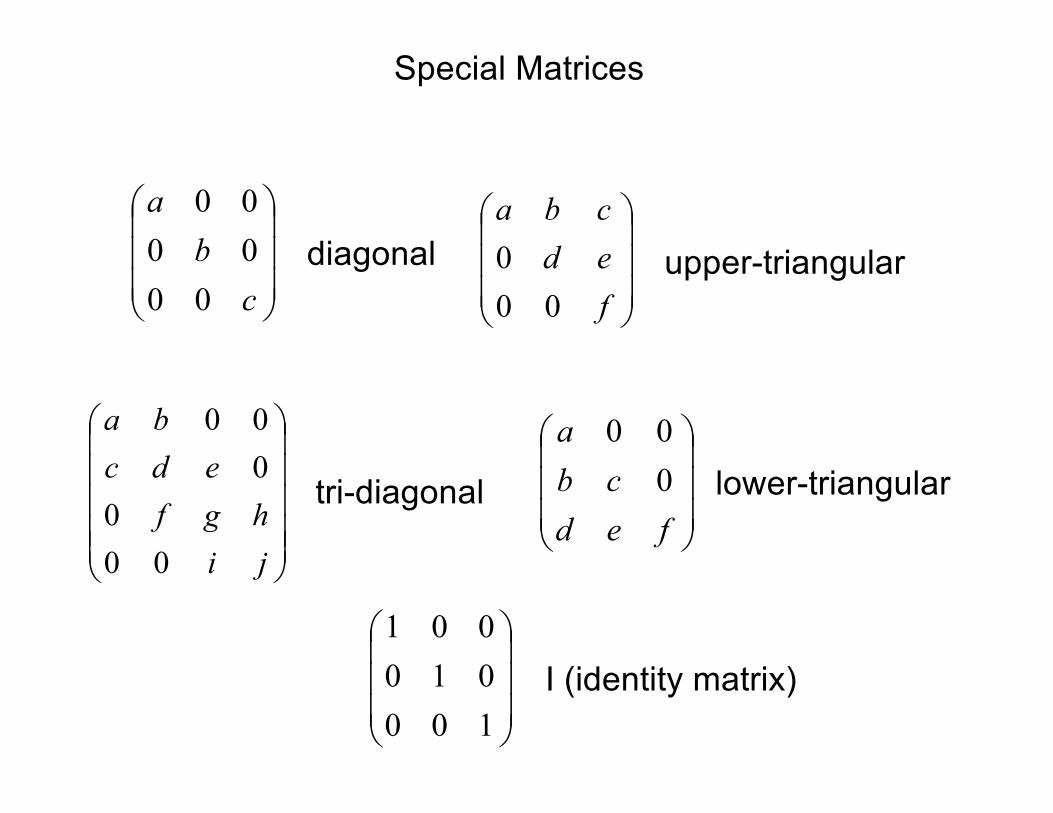
Special Matrices
÷÷÷
ø
ö
ççç
è
æ
fedcba
000
÷÷÷
ø
ö
ççç
è
æ
cb
a
000000
÷÷÷÷÷
ø
ö
ççççç
è
æ
jihgf
edcba
000
000
÷÷÷
ø
ö
ççç
è
æ
fedcb
a000
diagonal upper-triangular
tri-diagonal lower-triangular
÷÷÷
ø
ö
ççç
è
æ
100010001
I (identity matrix)
Special Matrices
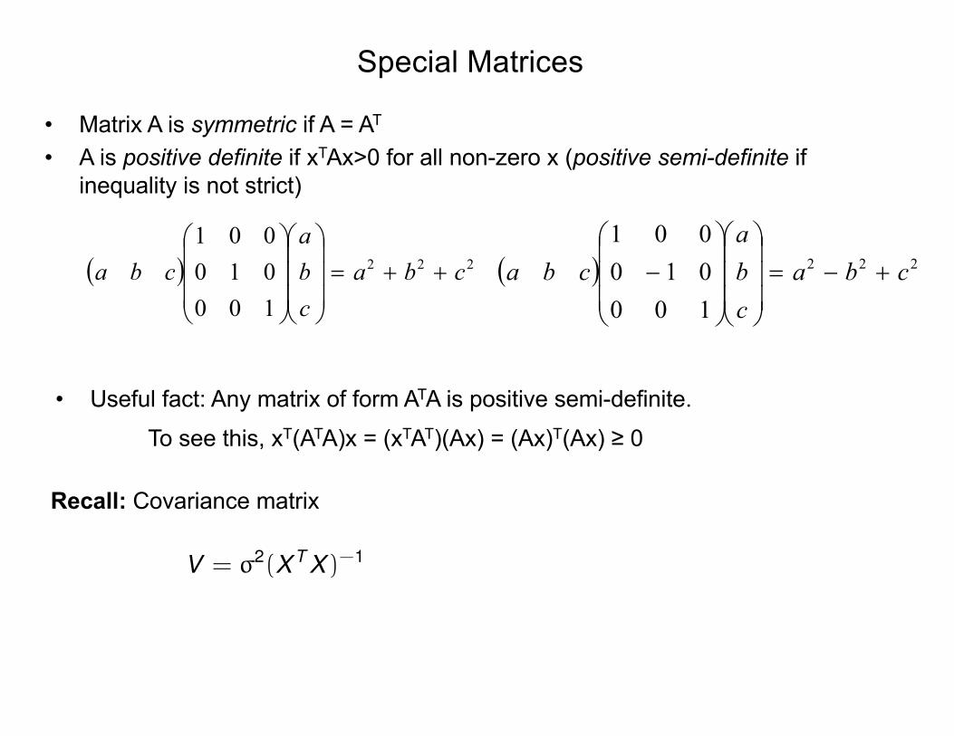
• Matrix A is symmetric if A = AT
• A is positive definite if xTAx>0 for all non-zero x (positive semi-definite if inequality is not strict)
( ) 222
100010001
cbacba
cba ++=÷÷÷
ø
ö
ççç
è
æ
÷÷÷
ø
ö
ççç
è
æ( ) 222
100010001
cbacba
cba +-=÷÷÷
ø
ö
ççç
è
æ
÷÷÷
ø
ö
ççç
è
æ-
• Useful fact: Any matrix of form ATA is positive semi-definite.To see this, xT(ATA)x = (xTAT)(Ax) = (Ax)T(Ax) ≥ 0
Recall: Covariance matrix
V = �2(X T X )-1
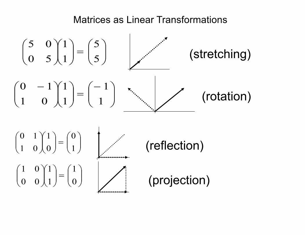
Matrices as Linear Transformations
÷÷ø
öççè
æ=÷÷
ø
öççè
æ÷÷ø
öççè
æ55
11
5005
(stretching)
÷÷ø
öççè
æ-=÷÷
ø
öççè
æ÷÷ø
öççè
æ -11
11
0110
(rotation)
÷÷ø
öççè
æ=÷÷
ø
öççè
æ÷÷ø
öççè
æ10
01
0110
(reflection)
÷÷ø
öççè
æ=÷÷
ø
öççè
æ÷÷ø
öççè
æ01
11
0001
(projection)
Linear Independence
÷÷÷
ø
ö
ççç
è
æ=
÷÷÷
ø
ö
ççç
è
æ
÷÷÷
ø
ö
ççç
è
æ
000
|||
|||
3
2
1
321
ccc
vvv
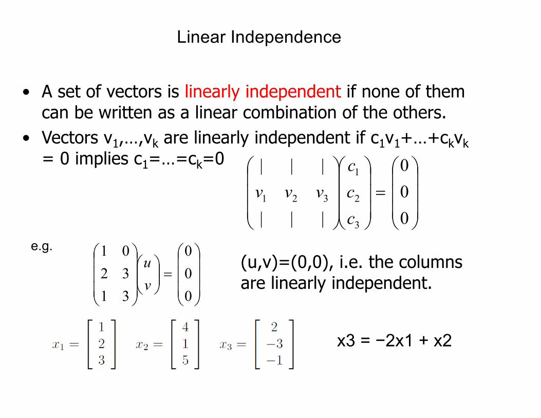
(u,v)=(0,0), i.e. the columns are linearly independent.
• A set of vectors is linearly independent if none of them can be written as a linear combination of the others.
• Vectors v1,…,vk are linearly independent if c1v1+…+ckvk= 0 implies c1=…=ck=0
÷÷÷
ø
ö
ççç
è
æ=÷÷
ø
öççè
æ
÷÷÷
ø
ö
ççç
è
æ
000
313201
vu
e.g.
x3 = −2x1 + x2
Basis Vectors
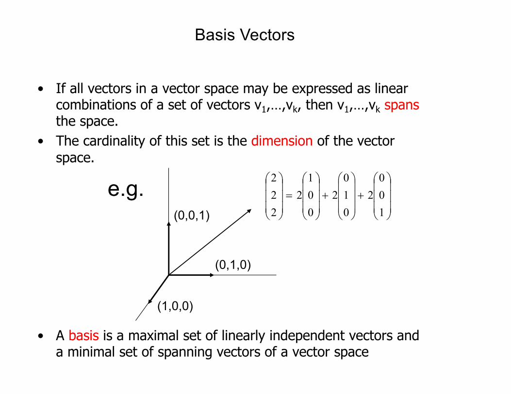
• If all vectors in a vector space may be expressed as linear combinations of a set of vectors v1,…,vk, then v1,…,vk spansthe space.
• The cardinality of this set is the dimension of the vector space.
• A basis is a maximal set of linearly independent vectors and a minimal set of spanning vectors of a vector space
÷÷÷
ø
ö
ççç
è
æ+
÷÷÷
ø
ö
ççç
è
æ+
÷÷÷
ø
ö
ççç
è
æ=
÷÷÷
ø
ö
ççç
è
æ
100
2010
2001
2222
(0,0,1)
(0,1,0)
(1,0,0)
e.g.
Basis Vectors
• An orthonormal basis consists of orthogonal vectors of unit length.Note:
÷÷÷
ø
ö
ççç
è
æ+
÷÷÷
ø
ö
ççç
è
æ+
÷÷÷
ø
ö
ççç
è
æ=
÷÷÷
ø
ö
ççç
è
æ
100
2010
2001
2222
(0,0,1)
(0,1,0)
(1,0,0)
(.1,.2,1)
(.3,1,0)(.9,.2,0)
÷÷÷
ø
ö
ççç
è
æ+
÷÷÷
ø
ö
ççç
è
æ+
÷÷÷
ø
ö
ççç
è
æ=
÷÷÷
ø
ö
ççç
è
æ
12.1.
2013.
29.102.9.
57.1222
Rank of a Matrix
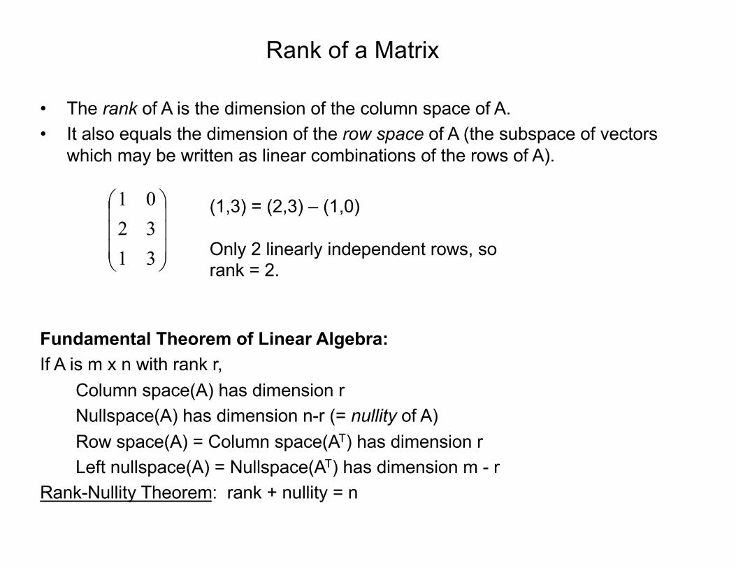
• The rank of A is the dimension of the column space of A.• It also equals the dimension of the row space of A (the subspace of vectors
which may be written as linear combinations of the rows of A).
÷÷÷
ø
ö
ççç
è
æ
313201 (1,3) = (2,3) – (1,0)
Only 2 linearly independent rows, so rank = 2.
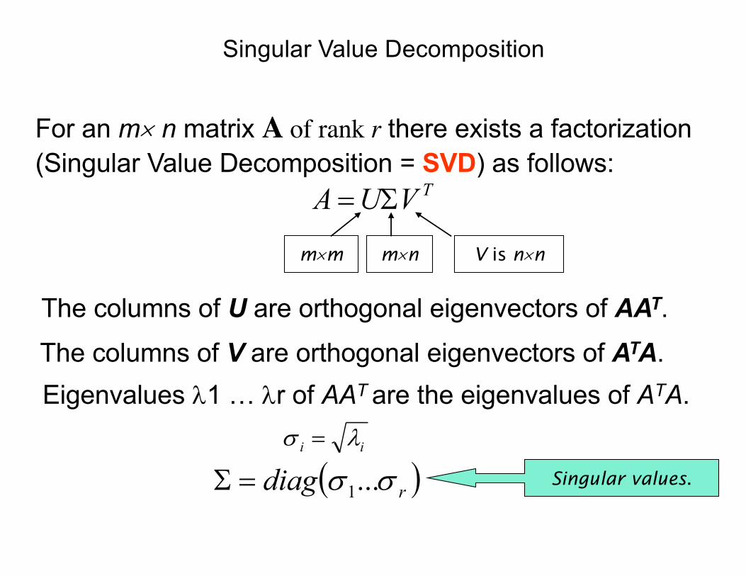
Fundamental Theorem of Linear Algebra:If A is m x n with rank r,
Column space(A) has dimension rNullspace(A) has dimension n-r (= nullity of A)Row space(A) = Column space(AT) has dimension rLeft nullspace(A) = Nullspace(AT) has dimension m - r
Rank-Nullity Theorem: rank + nullity = n
Matrix Inverse
• To solve Ax=b, we can write a closed-form solution if we can find a matrix A-1
such that AA-1 =A-1A=I (Identity matrix)• Then Ax=b iff x=A-1b:
x = Ix = A-1Ax = A-1b• A is non-singular iff A-1 exists iff Ax=b has a unique solution.• Note: If A-1,B-1 exist, then (AB)-1 = B-1A-1,
and (AT)-1 = (A-1)T
Note:
• For orthonormal matrices
A-1 = AT
Matrix Determinants
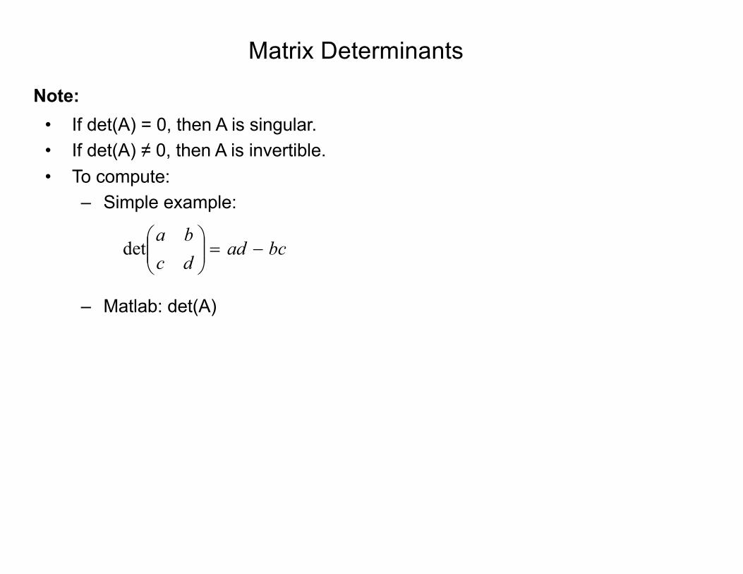
Note:• If det(A) = 0, then A is singular.• If det(A) ≠ 0, then A is invertible.• To compute:
– Simple example:
– Matlab: det(A)
bcaddcba
-=÷÷ø
öççè
ædet
MATLAB Interlude
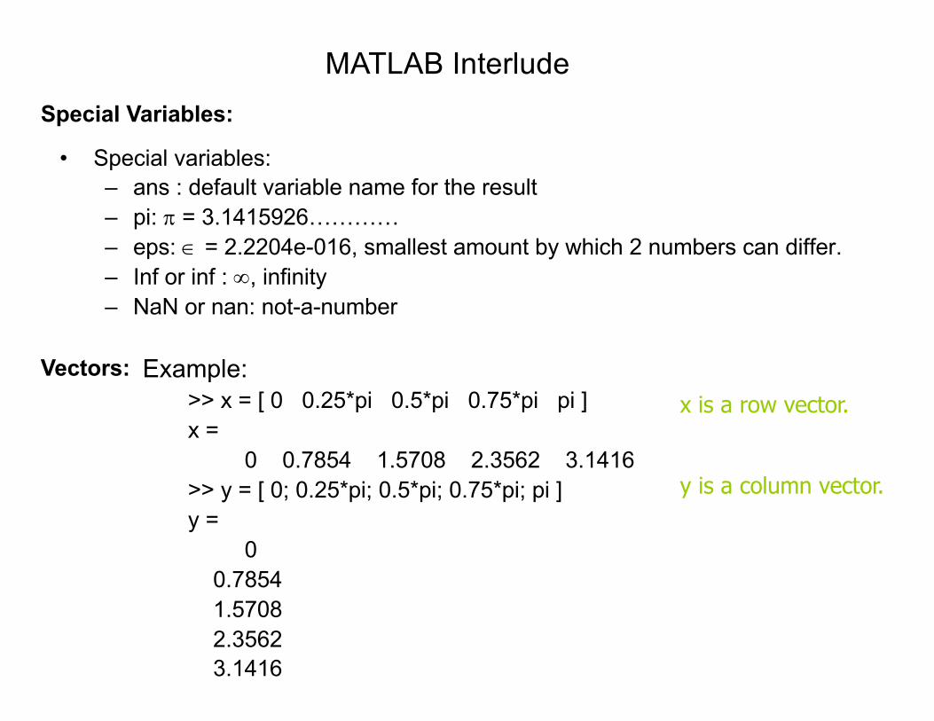
Special Variables:
• Special variables:– ans : default variable name for the result– pi: p = 3.1415926…………– eps: Î = 2.2204e-016, smallest amount by which 2 numbers can differ.– Inf or inf : ¥, infinity– NaN or nan: not-a-number
Vectors: Example:>> x = [ 0 0.25*pi 0.5*pi 0.75*pi pi ]x =
0 0.7854 1.5708 2.3562 3.1416>> y = [ 0; 0.25*pi; 0.5*pi; 0.75*pi; pi ]y =
00.78541.57082.35623.1416
x is a row vector.
y is a column vector.
Vectors
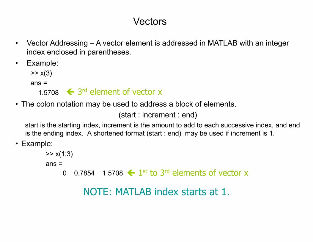
• Vector Addressing – A vector element is addressed in MATLAB with an integer index enclosed in parentheses.
• Example:>> x(3)ans =
1.5708
ç 1st to 3rd elements of vector x
• The colon notation may be used to address a block of elements.(start : increment : end)
start is the starting index, increment is the amount to add to each successive index, and end is the ending index. A shortened format (start : end) may be used if increment is 1.
• Example:>> x(1:3)ans =
0 0.7854 1.5708
NOTE: MATLAB index starts at 1.
ç 3rd element of vector x
Vectors
Some useful commands:
x = start:end create row vector x starting with start, counting by one, ending at end
x = start:increment:end create row vector x starting with start, counting by increment, ending at or before end
linspace(start,end,number) create row vector x starting with start, ending at end, having number elements
length(x) returns the length of vector x
y = x’ transpose of vector x
dot (x, y) returns the scalar dot product of the vector x and y.
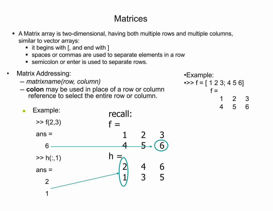
Matrices§ A Matrix array is two-dimensional, having both multiple rows and multiple columns,
similar to vector arrays:§ it begins with [, and end with ]§ spaces or commas are used to separate elements in a row§ semicolon or enter is used to separate rows.
•Example:•>> f = [ 1 2 3; 4 5 6]
f =1 2 34 5 6
• Matrix Addressing:-- matrixname(row, column)-- colon may be used in place of a row or column
reference to select the entire row or column.
recall:f =
1 2 34 5 6
h =2 4 61 3 5
n Example:
>> f(2,3)
ans =
6
>> h(:,1)
ans =
2
1
Matrices
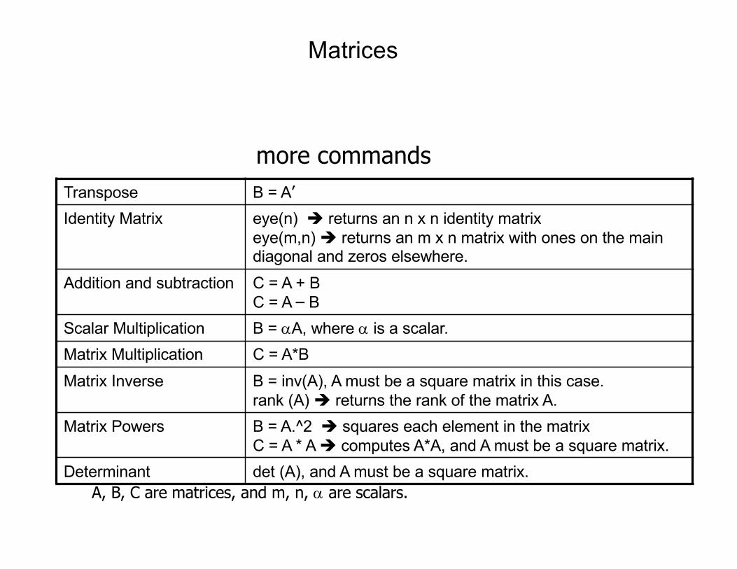
Transpose B = A’Identity Matrix eye(n) è returns an n x n identity matrix
eye(m,n) è returns an m x n matrix with ones on the main diagonal and zeros elsewhere.
Addition and subtraction C = A + BC = A – B
Scalar Multiplication B = aA, where a is a scalar.Matrix Multiplication C = A*BMatrix Inverse B = inv(A), A must be a square matrix in this case.
rank (A) è returns the rank of the matrix A.Matrix Powers B = A.^2 è squares each element in the matrix
C = A * A è computes A*A, and A must be a square matrix.Determinant det (A), and A must be a square matrix.
more commands
A, B, C are matrices, and m, n, a are scalars.
Matrices
>> A = [1 2;3 4]A =
1 2 3 4
>> B = [2 0;2 1]B =
2 0 2 1
>> A*Bans =
6 2 14 4
>> A.*Bans =
2 0 6 4
>> A = [1 2 3;0 2 0]A = �������������
������������������
>> B = [1;-1;0]B = �������������
>> A*Bans = �����������
Eigenvalues and Eigenvectors
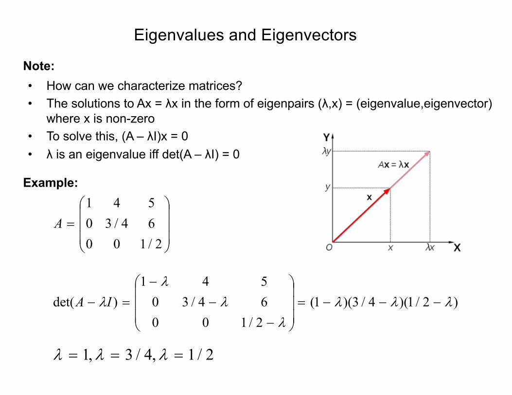
• How can we characterize matrices?• The solutions to Ax = λx in the form of eigenpairs (λ,x) = (eigenvalue,eigenvector)
where x is non-zero• To solve this, (A – λI)x = 0• λ is an eigenvalue iff det(A – λI) = 0
Note:
Example:
÷÷÷
ø
ö
ççç
è
æ=
2/10064/30541
A
)2/1)(4/3)(1(2/10064/30541
)det( llll
ll
l ---=÷÷÷
ø
ö
ççç
è
æ
--
-=- IA
2/1,4/3,1 === lll
Eigenvalues and Eigenvectors
Example:
÷÷ø
öççè
æ=
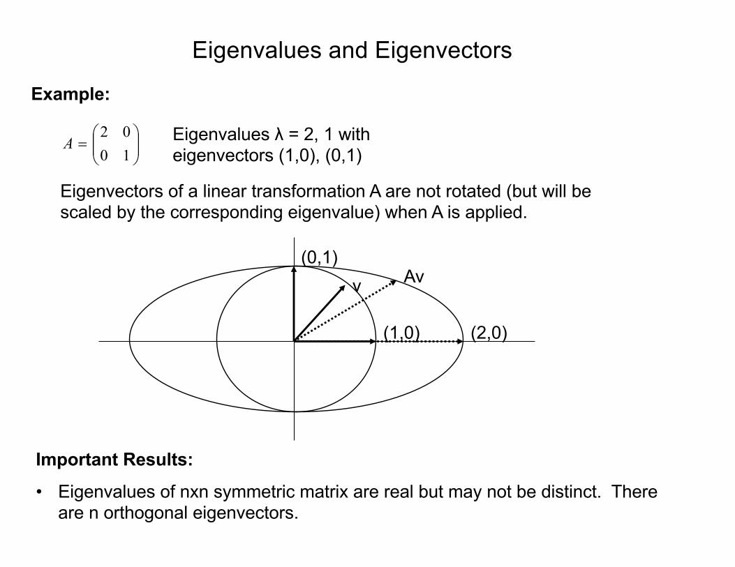
1002
A Eigenvalues λ = 2, 1 with eigenvectors (1,0), (0,1)
Eigenvectors of a linear transformation A are not rotated (but will be scaled by the corresponding eigenvalue) when A is applied.
(0,1)
(2,0)
v Av
(1,0)
Important Results:
• Eigenvalues of nxn symmetric matrix are real but may not be distinct. There are n orthogonal eigenvectors.
Eigenvalues and EigenvectorsImportant Results:
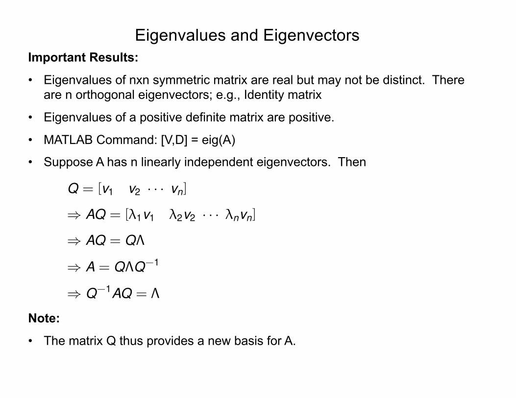
• Eigenvalues of nxn symmetric matrix are real but may not be distinct. There are n orthogonal eigenvectors; e.g., Identity matrix
• Eigenvalues of a positive definite matrix are positive.
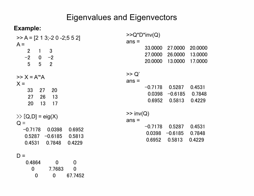
• MATLAB Command: [V,D] = eig(A)
• Suppose A has n linearly independent eigenvectors. Then
Q = [v1 v2 · · · vn]
) AQ = [�1v1 �2v2 · · · �nvn]
) AQ = Q⇤
) A = Q⇤Q-1
) Q-1AQ = ⇤
Note:
• The matrix Q thus provides a new basis for A.
Eigenvalues and EigenvectorsExample:>> A = [2 1 3;-2 0 -2;5 5 2]A = �������������
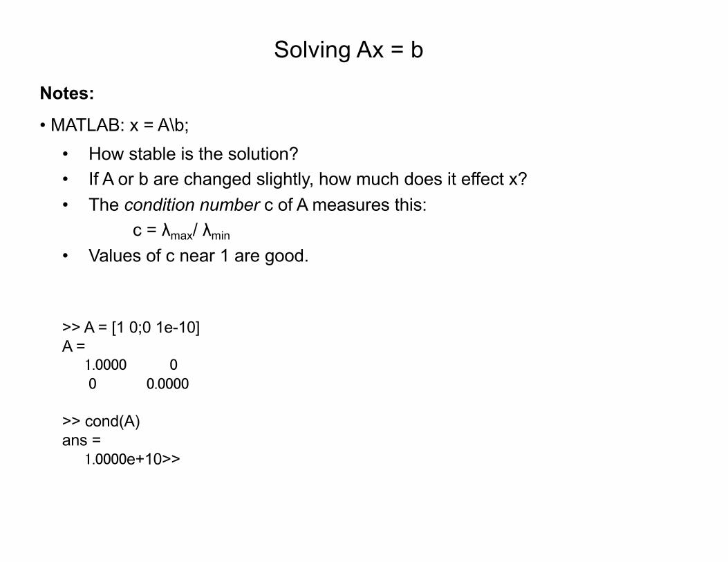
• MATLAB: x = A\b;• How stable is the solution?• If A or b are changed slightly, how much does it effect x?• The condition number c of A measures this:
c = λmax/ λmin
• Values of c near 1 are good.
>> A = [1 0;0 1e-10]A = ����������������������������� �������
>> cond(A)ans = ������e+10>>
MATLAB
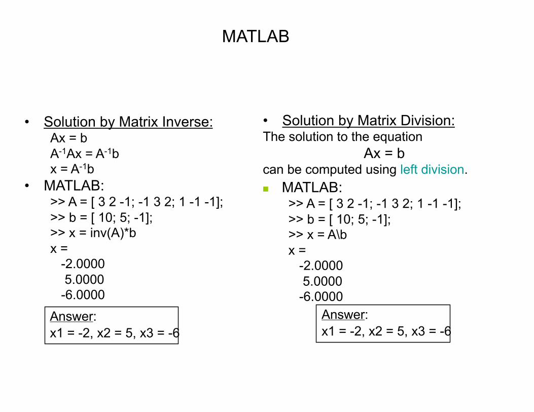
• Example: a system of 3 linear equations with 3 unknowns (x1, x2, x3):3x1 + 2x2 – x3 = 10-x1 + 3x2 + 2x3 = 5x1 – x2 – x3 = -1
• MATLAB:>> A = [ 3 2 -1; -1 3 2; 1 -1 -1];>> b = [ 10; 5; -1];>> x = inv(A)*bx =
-2.00005.0000-6.0000
Answer:x1 = -2, x2 = 5, x3 = -6
• Solution by Matrix Division:The solution to the equation
Ax = bcan be computed using left division.
Answer:x1 = -2, x2 = 5, x3 = -6
n MATLAB:>> A = [ 3 2 -1; -1 3 2; 1 -1 -1];>> b = [ 10; 5; -1];>> x = A\bx =
-2.00005.0000-6.0000
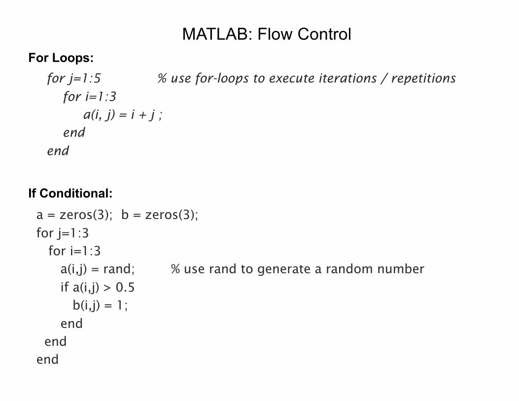
MATLAB: Flow Control
for j=1:5 % use for-loops to execute iterations / repetitions
for i=1:3a(i, j) = i + j ;
end
end
For Loops:
If Conditional:a = zeros(3); b = zeros(3);
for j=1:3 for i=1:3
a(i,j) = rand; % use rand to generate a random number
if a(i,j) > 0.5 b(i,j) = 1;
end end
end
MATLABCell Arrays:
A cell array is a special array of arrays. Each element of the cell array may point to a scalar, an array, or another cell array.>> C = cell(2, 3); % create 2x3 empty cell array >> M = magic(2);>> a = 1:3; b = [4;5;6]; s = 'This is a string.';
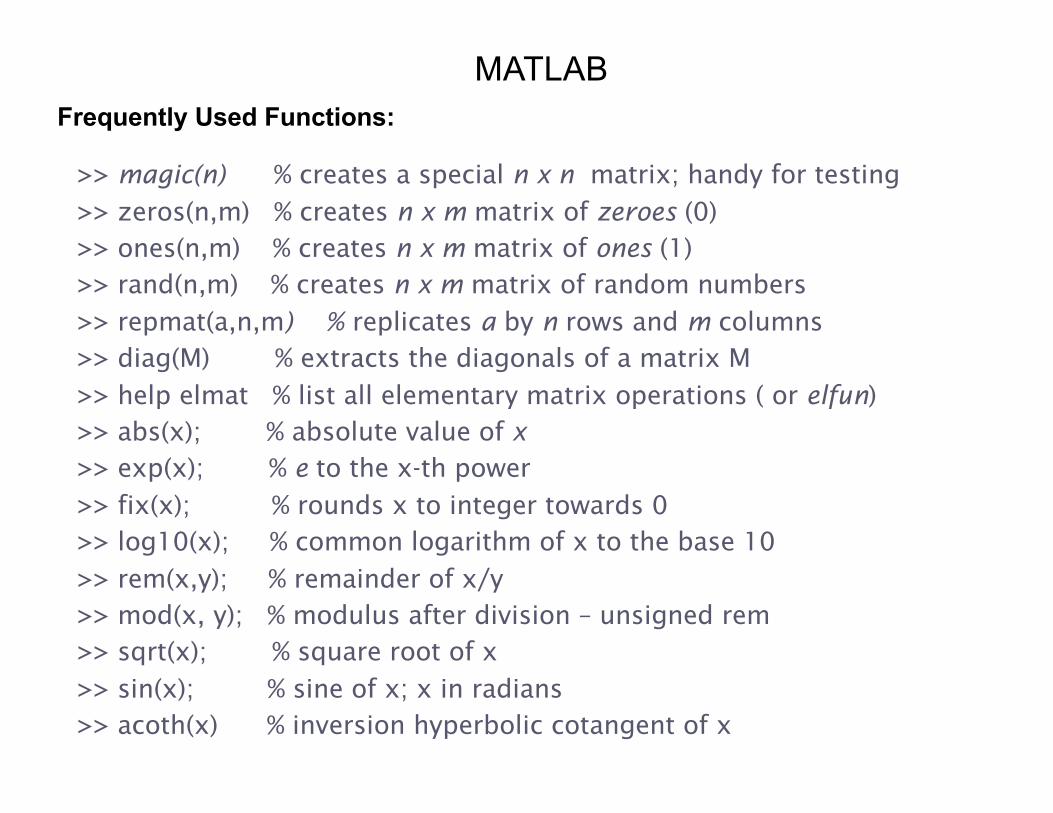
>> magic(n) % creates a special n x n matrix; handy for testing
>> zeros(n,m) % creates n x m matrix of zeroes (0)>> ones(n,m) % creates n x m matrix of ones (1)>> rand(n,m) % creates n x m matrix of random numbers
>> repmat(a,n,m) % replicates a by n rows and m columns>> diag(M) % extracts the diagonals of a matrix M
>> help elmat % list all elementary matrix operations ( or elfun)>> abs(x); % absolute value of x >> exp(x); % e to the x-th power
>> fix(x); % rounds x to integer towards 0 >> log10(x); % common logarithm of x to the base 10
>> rem(x,y); % remainder of x/y>> mod(x, y); % modulus after division – unsigned rem>> sqrt(x); % square root of x
>> sin(x); % sine of x; x in radians >> acoth(x) % inversion hyperbolic cotangent of x
PlottingLine Plot:
>> t = 0:pi/100:2*pi;>> y = sin(t);>> plot(t,y)>> xlabel(‘t’);>> ylabel(‘sin(t)’);>> title(‘The plot of t vs sin(t)’);
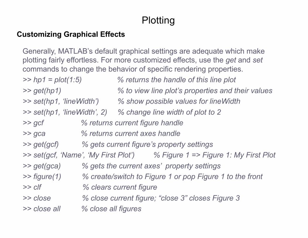
PlottingCustomizing Graphical Effects
Generally, MATLAB’s default graphical settings are adequate which make plotting fairly effortless. For more customized effects, use the get and setcommands to change the behavior of specific rendering properties.>> hp1 = plot(1:5) % returns the handle of this line plot>> get(hp1) % to view line plot’s properties and their values>> set(hp1, ‘lineWidth’) % show possible values for lineWidth>> set(hp1, ‘lineWidth’, 2) % change line width of plot to 2>> gcf % returns current figure handle>> gca % returns current axes handle>> get(gcf) % gets current figure’s property settings>> set(gcf, ‘Name’, ‘My First Plot’) % Figure 1 => Figure 1: My First Plot>> get(gca) % gets the current axes’ property settings>> figure(1) % create/switch to Figure 1 or pop Figure 1 to the front >> clf % clears current figure>> close % close current figure; “close 3” closes Figure 3>> close all % close all figures
PlottingSurface Plot
>> Z = peaks; % generate data for plot; peaks returns function values>> surf(Z) % surface plot of Z