94
MATLAB Signal Processing Toolbox Greg Reese, Ph.D Research Computing Support Group Academic Technology Services Miami University October 2013

MATLAB Signal
Processing Toolbox
Greg Reese, Ph.D
Research Computing Support Group
Academic Technology Services
Miami University
October 2013

MATLAB Signal
Processing Toolbox
© 2013 Greg Reese. All rights reserved 2

Toolbox
3
Toolbox
• Collection of code devoted to solving
problems in one field of research
• Can be purchased from MATLAB
• Can be purchased from third parties
• Can be obtained for free from third parties
Toolbox
4
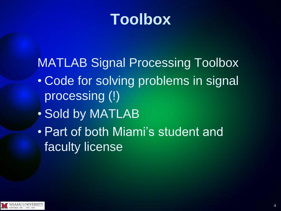
MATLAB Signal Processing Toolbox
• Code for solving problems in signal
processing (!)
• Sold by MATLAB
• Part of both Miami’s student and
faculty license

Overview
5
MATLAB divides Signal Processing
Toolbox as follows
• Waveforms – Pulses, modulated signals, peak-to-peak and RMS
amplitude, rise time/fall time, overshoot/undershoot
• Convolution and Correlation – Linear and circular convolution, autocorrelation,
autocovariance, cross-correlation, cross-covariance
• Transforms – Fourier transform, chirp z-transform, DCT, Hilbert
transform, cepstrum, Walsh-Hadamard transform

Overview
6
• Analog and Digital Filters – Analog filter design, frequency transformations, FIR and IIR
filters, filter analysis, filter structures
• Spectral Analysis – Nonparametric and parametric spectral estimation, high
resolution spectral estimation
• Parametric Modeling and Linear
Prediction – Autoregressive (AR) models, linear predictive coding (LPC),
Levinson-Durbin recursion
• Multirate Signal Processing – Downsampling, upsampling, resampling, anti-aliasing filter,
interpolation, decimation

Overview
7
Will look very briefly at
• Analog and Digital Filters
• Spectral Analysis
• Parametric Modeling and Linear Prediction
• Multirate Signal Processing
Will look in more depth at
• Waveforms
• Convolution and Correlation

Analog and Digital Filters
8
Toolbox especially good for those serious
about their filter design!
Analog filters
• Standard filters
– Bessel, Butterworth, Chebyshev, Elliptic
• Filter transforms
– Low pass to: bandpass, bandstop, or highpass
– Change cutoff frequency of lowpass
• Analog to digital filter conversion
– Bilinear transformation
Analog and Digital Filters
9
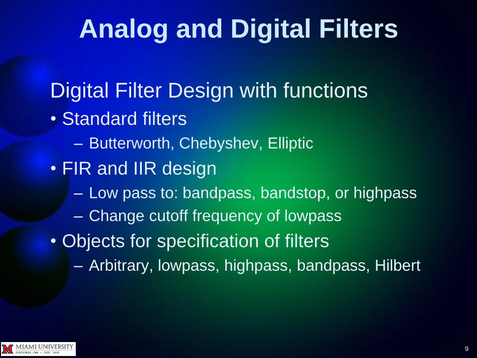
Digital Filter Design with functions
• Standard filters
– Butterworth, Chebyshev, Elliptic
• FIR and IIR design
– Low pass to: bandpass, bandstop, or highpass
– Change cutoff frequency of lowpass
• Objects for specification of filters
– Arbitrary, lowpass, highpass, bandpass, Hilbert
Analog and Digital Filters
10
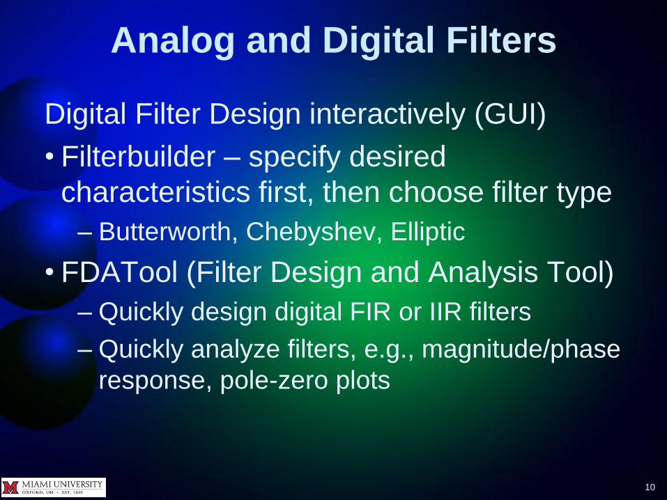
Digital Filter Design interactively (GUI)
• Filterbuilder – specify desired
characteristics first, then choose filter type
– Butterworth, Chebyshev, Elliptic
• FDATool (Filter Design and Analysis Tool)
– Quickly design digital FIR or IIR filters
– Quickly analyze filters, e.g., magnitude/phase
response, pole-zero plots

Analog and Digital Filters
11
SPTool – composite of four tools
1. Signal Browser – analyze signals
2. FDATool
3. FVTool (Filter Visualization Tool) –
analyze filter characteristics
4. Spectrum Viewer – spectral analysis

Analog and Digital Filters
12
Digital Filter Analysis
• Magnitude and phase response, impulse
response, group delay, pole-zero plot
Digital Filter Implementation
• Filtering, direct form, lattice, biquad, state-
space structures
Spectral Analysis
13
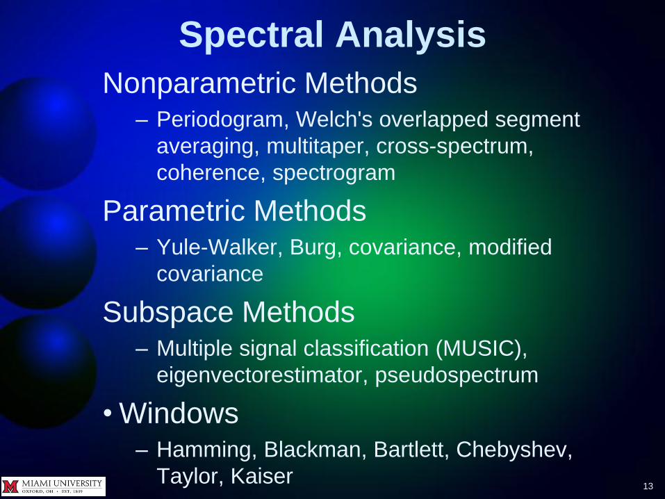
Nonparametric Methods – Periodogram, Welch's overlapped segment
averaging, multitaper, cross-spectrum,
coherence, spectrogram
Parametric Methods – Yule-Walker, Burg, covariance, modified
covariance
Subspace Methods – Multiple signal classification (MUSIC),
eigenvectorestimator, pseudospectrum
• Windows – Hamming, Blackman, Bartlett, Chebyshev,
Taylor, Kaiser

Parametric Modeling and
Linear Prediction
14
Parametric Modeling
• AR, ARMA, frequency response
modeling
Linear Predictive Waveforms
• Linear predictive coefficients (LPC), line
spectral frequencies (LSF), reflection
coefficients (RC), Levinson-Durbin
recursion

Multirate Signal Processing
15
Multirate signal processing
– Downsampling, upsampling, resampling,
anti-aliasing filter, interpolation, decimation

Waveforms
16
Waveforms part of toolbox lets you create
many commonly used signals, which you
can use to study models programmed in
MATLAB
Uses of waveforms
• Testing – E.g., have simple waveform and can analytically
determine model’s output. Use toolbox to create that
waveform, run it through MATLAB model, confirm
result
Waveforms
17
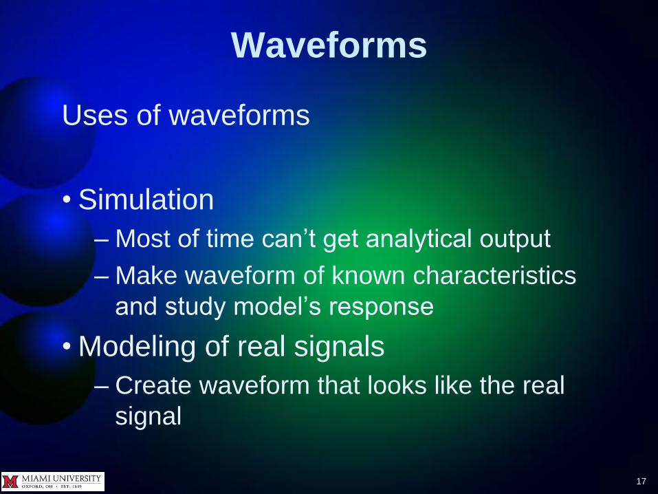
Uses of waveforms
• Simulation
– Most of time can’t get analytical output
– Make waveform of known characteristics
and study model’s response
• Modeling of real signals
– Create waveform that looks like the real
signal

Waveforms
18
Time vectors
Digital signals usually sampled from
analog at fixed intervals Δt . Want time
axis with N points
0 1Δt 2Δt … (N-2)Δt (N-1)Δt
Waveforms
19
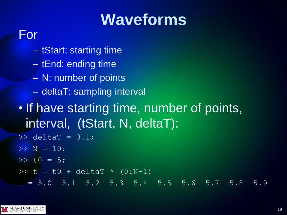
For – tStart: starting time
– tEnd: ending time
– N: number of points
– deltaT: sampling interval
• If have starting time, number of points,
interval, (tStart, N, deltaT): >> deltaT = 0.1;
>> N = 10;
>> t0 = 5;
>> t = t0 + deltaT * (0:N-1)
t = 5.0 5.1 5.2 5.3 5.4 5.5 5.6 5.7 5.8 5.9
Waveforms
20
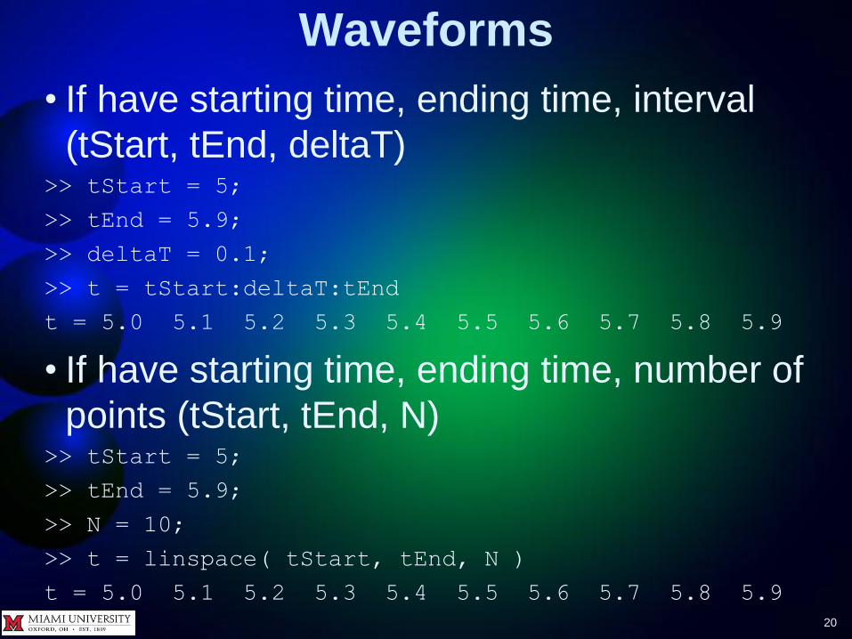
• If have starting time, ending time, interval
(tStart, tEnd, deltaT) >> tStart = 5;
>> tEnd = 5.9;
>> deltaT = 0.1;
>> t = tStart:deltaT:tEnd
t = 5.0 5.1 5.2 5.3 5.4 5.5 5.6 5.7 5.8 5.9
• If have starting time, ending time, number of
points (tStart, tEnd, N) >> tStart = 5;
>> tEnd = 5.9;
>> N = 10;
>> t = linspace( tStart, tEnd, N )
t = 5.0 5.1 5.2 5.3 5.4 5.5 5.6 5.7 5.8 5.9

Waveforms
21
In multichannel processing, a number of
signals are gathered at the same time
• Will assume all sampled at same time and
same rate
Signal processing toolbox, and MATLAB
in general, treats each column of a
matrix (2D array) as an independent column vector

Waveforms
22
Example >> M = [ 1:3; 4:6; 7:9; 10:12 ]
M = 1 2 3
4 5 6
7 8 9
10 11 12
>> mean( M )
ans =
5.5000 6.5000 7.5000
Result is mean of each column

Waveforms
23
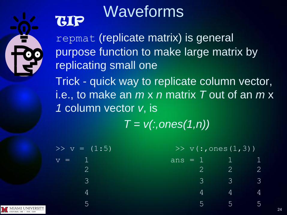
TIP
Make time vector be a column vector
• Any vectors created from time vector
will also be column vectors and so
can be processed more easily >> t = t >> y = abs( t - 3 )
t = 1 y = 2
2 1
3 0
4 1
5 2
6 3
Column vector begeteth column vector
Waveforms
24
TIP
repmat (replicate matrix) is general
purpose function to make large matrix by
replicating small one
Trick - quick way to replicate column vector,
i.e., to make an m x n matrix T out of an m x
1 column vector v, is
T = v(:,ones(1,n))
>> v = (1:5) >> v(:,ones(1,3))
v = 1 ans = 1 1 1
2 2 2 2
3 3 3 3
4 4 4 4
5 5 5 5

Waveforms
25
TIP
Trick - quick way to replicate row vector,
i.e., to make an m x n matrix T out of an 1 x
n row vector v, is
T = v(ones(m,1),:)
>> v = 1:3 >> T = v( ones(6,1), : )
v = 1 2 3 ans = 1 2 3
2 1 2 3
3 1 2 3
4 1 2 3
5 1 2 3
1 2 3

Waveforms
26
TIP
Can use preceding two tips to make
multichannel signal, e.g.,
Simulate the multichannel signal
sin(2πt), sin(2πt/2), sin(2πt/3),
sin(2πt/4) sampled for one second
at one-tenth second per sample

Waveforms
27
TIP >> t = (0:0.1:1)'
t = 0
0.1000
0.2000
0.3000
0.4000
0.5000
0.6000
0.7000
0.8000
0.9000
1.0000

Waveforms
28
TIP >> T = t(:,ones(1,4))
T = 0 0 0 0
0.1000 0.1000 0.1000 0.1000
0.2000 0.2000 0.2000 0.2000
0.3000 0.3000 0.3000 0.3000
0.4000 0.4000 0.4000 0.4000
0.5000 0.5000 0.5000 0.5000
0.6000 0.6000 0.6000 0.6000
0.7000 0.7000 0.7000 0.7000
0.8000 0.8000 0.8000 0.8000
0.9000 0.9000 0.9000 0.9000
1.0000 1.0000 1.0000 1.0000

Waveforms
29
TIP >> M = T ./ C
M =
0 0 0 0
0.1000 0.0500 0.0333 0.0250
0.2000 0.1000 0.0667 0.0500
0.3000 0.1500 0.1000 0.0750
0.4000 0.2000 0.1333 0.1000
0.5000 0.2500 0.1667 0.1250
0.6000 0.3000 0.2000 0.1500
0.7000 0.3500 0.2333 0.1750
0.8000 0.4000 0.2667 0.2000
0.9000 0.4500 0.3000 0.2250
1.0000 0.5000 0.3333 0.2500
Waveforms
30
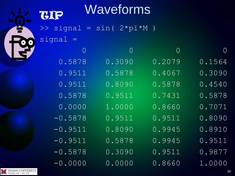
TIP >> signal = sin( 2*pi*M )
signal =
0 0 0 0
0.5878 0.3090 0.2079 0.1564
0.9511 0.5878 0.4067 0.3090
0.9511 0.8090 0.5878 0.4540
0.5878 0.9511 0.7431 0.5878
0.0000 1.0000 0.8660 0.7071
-0.5878 0.9511 0.9511 0.8090
-0.9511 0.8090 0.9945 0.8910
-0.9511 0.5878 0.9945 0.9511
-0.5878 0.3090 0.9511 0.9877
-0.0000 0.0000 0.8660 1.0000
Waveforms
31
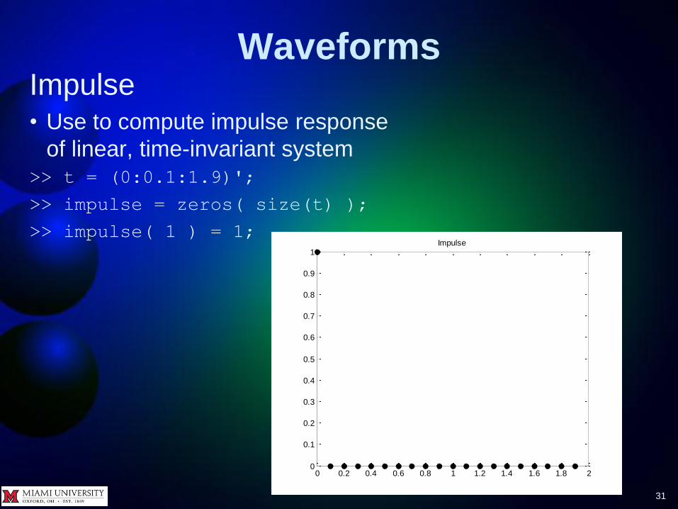
Impulse • Use to compute impulse response
of linear, time-invariant system >> t = (0:0.1:1.9)';
>> impulse = zeros( size(t) );
>> impulse( 1 ) = 1;
0 0.2 0.4 0.6 0.8 1 1.2 1.4 1.6 1.8 20
0.1
0.2
0.3
0.4
0.5
0.6
0.7
0.8
0.9
1Impulse
Waveforms
32
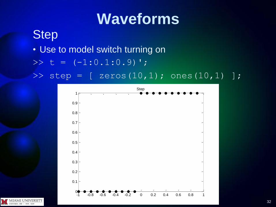
Step • Use to model switch turning on
>> t = (-1:0.1:0.9)';
>> step = [ zeros(10,1); ones(10,1) ];
-1 -0.8 -0.6 -0.4 -0.2 0 0.2 0.4 0.6 0.8 10
0.1
0.2
0.3
0.4
0.5
0.6
0.7
0.8
0.9
1Step
Waveforms
33
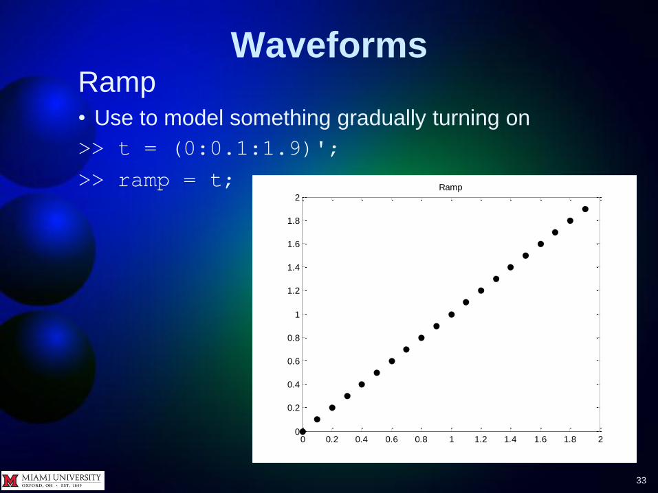
Ramp • Use to model something gradually turning on
>> t = (0:0.1:1.9)';
>> ramp = t;
0 0.2 0.4 0.6 0.8 1 1.2 1.4 1.6 1.8 20
0.2
0.4
0.6
0.8
1
1.2
1.4
1.6
1.8
2Ramp
Autocorrelation
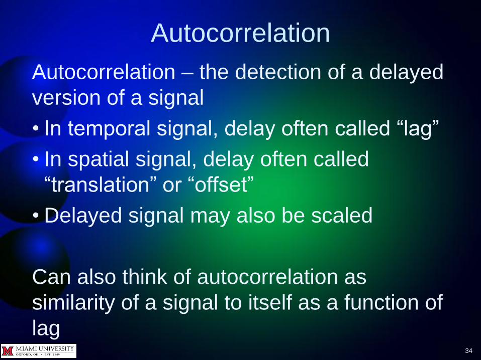
34
Autocorrelation – the detection of a delayed
version of a signal
• In temporal signal, delay often called “lag”
• In spatial signal, delay often called
“translation” or “offset”
• Delayed signal may also be scaled
Can also think of autocorrelation as
similarity of a signal to itself as a function of
lag

Autocorrelation
35
Autocorrelation and cross-correlation
• Common in both signal processing
and statistics
• Definitions and uses are different
• When looking for help on these
topics, make sure you’re looking at
a signal-processing source

Autocorrelation
36
Examples of autocorrelation of digital signals
• Radar – determine distance to object
• Sonar – determine distance to object
• Music
– Determine tempo
– Detect and estimate pitch
• Astronomy – Find rotation frequency of pulsars

Autocorrelation
37
Examples of spatial autocorrelation
• Optical Character Recognition (OCR) – reading
text from images of writing/printing
• X-ray diffraction – helps recover the "Fourier
phase information" on atom positions
• Statistics – helps estimate mean value
uncertainties when sampling a heterogeneous
population
• Astrophysics – used to study and characterize
the spatial distribution of galaxies

Autocorrelation
38
Examples of optical autocorrelation
• Measurement of optical spectra and of very
short-duration light pulses produced by lasers
• Analysis of dynamic light scattering data to
determine particle size distributions
• The small-angle X-ray scattering intensity of
some systems related to the spatial
autocorrelation function of the electron density
• In optics, normalized autocorrelations and
cross-correlations give the degree of
coherence of an electromagnetic field

Autocorrelation
39
Typical use
• Blip sent to object
• Small blip reflected from
object back to sender
• Use autocorrelation to detect
small blip at some lag
• Know velocity of blip in medium so total
distance blip traveled is
distance = velocity * lag
• Distance is round trip, so
object distance/2 away

Autocorrelation
40
Autocorrelation
• Multiply and sum. Result is autocorrelation at
that point
• Slide over one, multiply and sum
10 10 10
0 0 0 0 0 1 1 1 0 0
x x x
10∙0 + 10∙0 + 10∙0 = 0
10 10 10
x x x
10∙0 + 10∙0 + 10∙0 = 0

Autocorrelation
41
Autocorrelation
• Repeat, sliding in both directions until have
covered all positions
• What happens when go
past end?
10 10 10
0 0 0 0 0 1 1 1 0 0
x x x
10∙0 + 10∙0 + ?
?
Autocorrelation
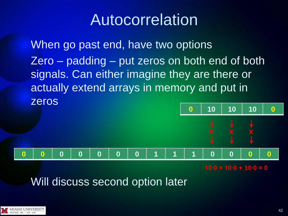
42
When go past end, have two options
Zero – padding – put zeros on both end of both
signals. Can either imagine they are there or
actually extend arrays in memory and put in
zeros
Will discuss second option later
0 10 10 10 0
0 0 0 0 0 0 0 1 1 1 0 0 0 0
x x x
10∙0 + 10∙0 + 10∙0 = 0

Autocorrelation
43
Suppose the real discrete-time signal x[n] has
L points and the real discrete-time signal y[n]
has N points, with L ≤ N. The autocorrelation of
x and y is
𝑅𝑥𝑦 𝑚 = 𝑥 𝑛 + 𝑚 𝑦[𝑛]
𝐿−𝑚−1
𝑛=0
for m = -(N-1), -(N-2), …, -1, 0, 1, 2, …, L-1
Autocorrelation
44
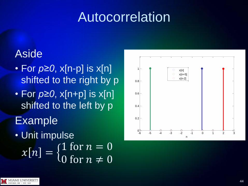
Aside
• For p≥0, x[n-p] is x[n]
shifted to the right by p
• For p≥0, x[n+p] is x[n]
shifted to the left by p
Example
• Unit impulse
𝑥 𝑛 = 1 for 𝑛 = 00 for 𝑛 ≠ 0
-6 -5 -4 -3 -2 -1 0 1 2 30
0.2
0.4
0.6
0.8
1
n
x[n]
x[n+5]
x[n-2]
Autocorrelation
45
TRY IT
At time n=0 a transmitter sends out a
pulse of amplitude ten and duration 3.
At time time n=5 it gets back the
reflected pulse with the same duration
but one tenth the amplitude. What is the
autocorrelation?
Autocorrelation
46
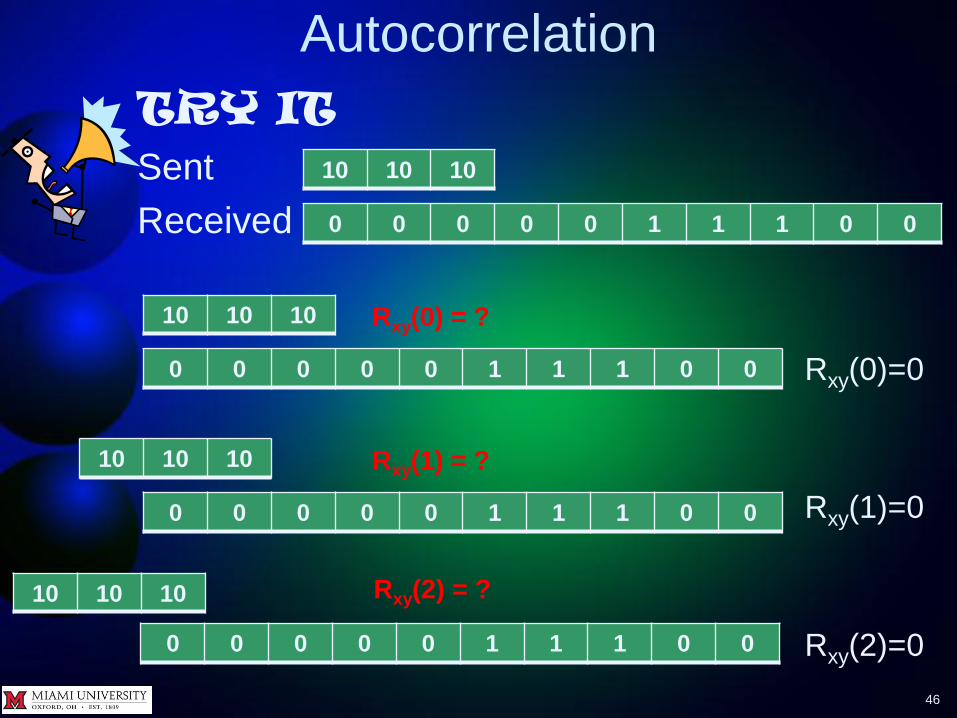
TRY IT
Sent
Received
Rxy(0)=0
Rxy(1)=0
Rxy(2)=0
10 10 10
0 0 0 0 0 1 1 1 0 0
10 10 10
0 0 0 0 0 1 1 1 0 0
Rxy(0) = ?
10 10 10
0 0 0 0 0 1 1 1 0 0
Rxy(1) = ?
10 10 10
0 0 0 0 0 1 1 1 0 0
Rxy(2) = ?

Autocorrelation
47
TRY IT
Rxy(-1)=0
Rxy(-2)=0
Rxy(-3)=10
Rxy(-4)=20
Rxy(-5)=30
10 10 10
0 0 0 0 0 1 1 1 0 0
Rxy(-1) = ?
10 10 10
0 0 0 0 0 1 1 1 0 0
Rxy(-2) = ?
10 10 10
0 0 0 0 0 1 1 1 0 0
Rxy(-3) = ?
10 10 10
0 0 0 0 0 1 1 1 0 0
Rxy(-4) = ?
10 10 10
0 0 0 0 0 1 1 1 0 0
Rxy(-5) = ?

Autocorrelation
48
TRY IT
Rxy(-6)=20
Rxy(-7)=10
Rxy(-8)=0
Rxy(-9)=0
10 10 10
0 0 0 0 0 1 1 1 0 0
Rxy(-6) = ?
10 10 10
0 0 0 0 0 1 1 1 0 0
Rxy(-7) = ?
10 10 10
0 0 0 0 0 1 1 1 0 0
Rxy(-8) = ?
10 10 10
0 0 0 0 0 1 1 1 0 0
Rxy(-9) = ?
Autocorrelation
49
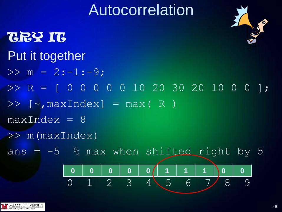
TRY IT
Put it together
>> m = 2:-1:-9;
>> R = [ 0 0 0 0 0 10 20 30 20 10 0 0 ];
>> [~,maxIndex] = max( R )
maxIndex = 8
>> m(maxIndex)
ans = -5 % max when shifted right by 5
0 1 2 3 4 5 6 7 8 9
0 0 0 0 0 1 1 1 0 0

Autocorrelation
50
TRY IT >> plot( -m, R, ‘o’ )
Note shape is a triangle, not a rectangle,
which is shape of pulse. Autocorrelation
detects signal of given shape – it does not
replicate signal
-2 0 2 4 6 8 100
5
10
15
20
25
30
Lag m
Auto
corr
ela
tion(m
)
Autocorrelation
51
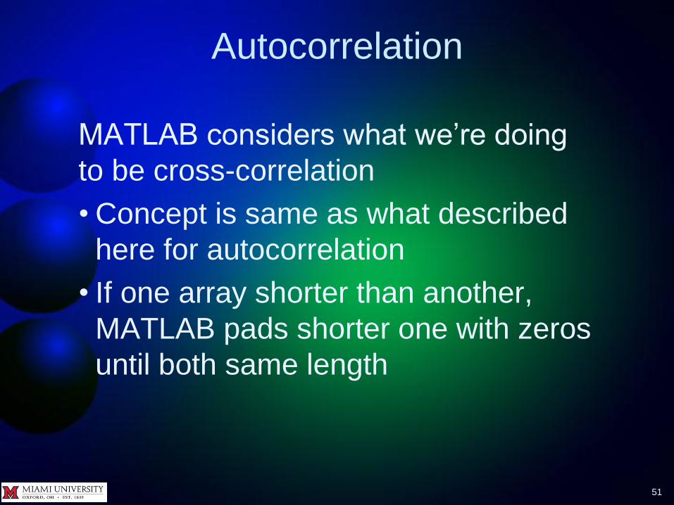
MATLAB considers what we’re doing
to be cross-correlation
• Concept is same as what described
here for autocorrelation
• If one array shorter than another,
MATLAB pads shorter one with zeros
until both same length

Autocorrelation
52
To compute cross-correlation of
vectors x and y in MATLAB, use
c = xcorr( x, y )
where
• c is a vector with 2N-1 elements
• N is length of longer of x and y
If m is lag as previously defined, c(k)
is autocorrelation for lag m = k - N
Autocorrelation
53
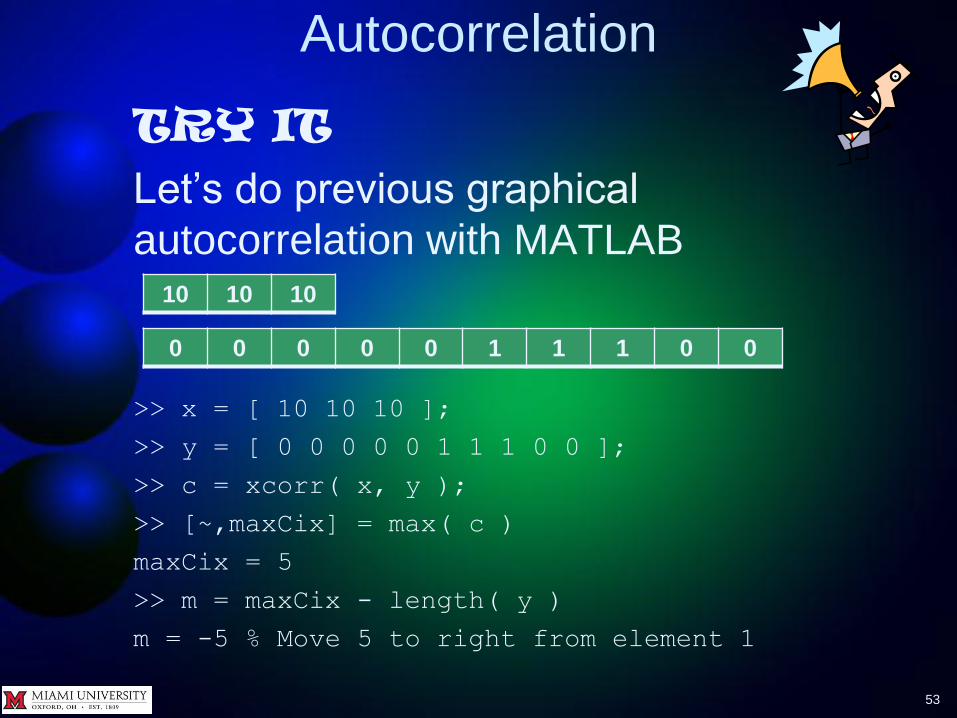
TRY IT
Let’s do previous graphical
autocorrelation with MATLAB
>> x = [ 10 10 10 ];
>> y = [ 0 0 0 0 0 1 1 1 0 0 ];
>> c = xcorr( x, y );
>> [~,maxCix] = max( c )
maxCix = 5
>> m = maxCix - length( y )
m = -5 % Move 5 to right from element 1
10 10 10
0 0 0 0 0 1 1 1 0 0

Autocorrelation
54
TRY IT
Example of finding signal buried in noise
1. Make a sine wave with a period of 20 and
amplitude of 100 >> wave = 100 * sin( 2*pi*(0:19)/20 );
2. Reset random number generator
(so we all get the same random numbers) >> rng default
3. Make 500 points of noise with randn and
variance 75% of wave amplitude noisyWave = 75 * randn( 1, 500 );

Autocorrelation
55
TRY IT
4. Pick a random spot to place the wave,
ensuring that the whole wave fits in ix = randi( [ 1, 481 ] );
5. Add the wave to the noise noisyWave(ix:ix+19)=noisyWave(ix:ix+19)+wave;
Plot wave in noise. Is wave visible? plot( noisyWave )
6. Compute autocorrelation
>> c = xcorr( wave, noisyWave );
0 50 100 150 200 250 300 350 400 450 500-300
-200
-100
0
100
200
300
Autocorrelation
56
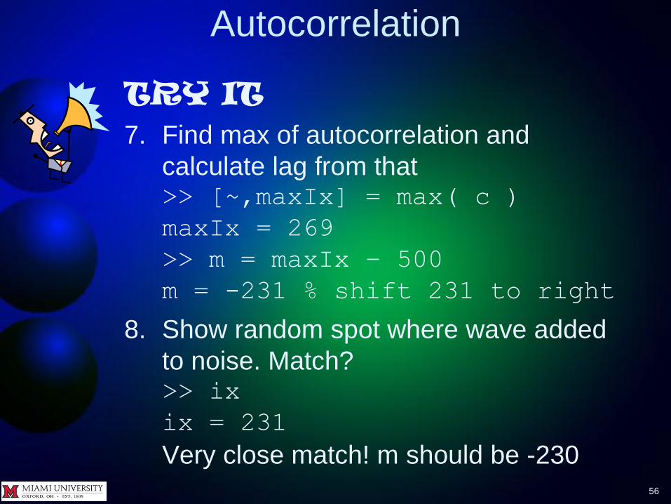
TRY IT
7. Find max of autocorrelation and
calculate lag from that >> [~,maxIx] = max( c )
maxIx = 269
>> m = maxIx – 500
m = -231 % shift 231 to right
8. Show random spot where wave added
to noise. Match? >> ix
ix = 231
Very close match! m should be -230

Autocorrelation
57
TRY IT
9. For grins, plot autocorrelation >> lags = -499:499;
>> plot( lags, c )
Why is almost
all of right
size zero? • Right side
corresponds to
shifting left and once
shift wave more than
20, rest of wave
is zeros -500 -400 -300 -200 -100 0 100 200 300 400 500-8
-6
-4
-2
0
2
4
6
8x 10
4

Correlation
58
Questions?

Convolution
59
convolution
• Uses – Polynomial multiplication
– LTI response
– Joint PDF
• Linear and circular – Explain, show when equivalent (padding), good for
computing convolution with fft. Do example with
tic,toc, time-domain convolution vs. fft,ifft, see cconv

Convolution
60
Applications of convolution
• Acoustics – reverberation is the convolution of
the original sound with echoes from objects
surrounding the sound source
• Computational fluid dynamics – the large eddy
simulation (LES) turbulence model uses
convolution to lower the range of length scales
necessary in computation and thereby reducing
computational cost
• Probability – probability distribution of the sum
of two independent random variables is the
convolution of their individual distributions

Convolution
61
Applications of convolution
• Spectroscopy – line broadening can be due to
the Doppler effect and/or collision broadening.
The effect due to both is the convolution of the
two effects
• Electronic music – imposition of a rhythmic
structure on a sound done by convolution
• Image processing – blurring, sharpening, and
edge enhancement done by convolution
• Numerical computation – can multiply
polynomials quickly with convolution
Convolution
62
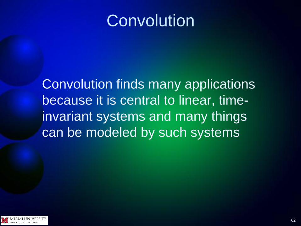
Convolution finds many applications
because it is central to linear, time-
invariant systems and many things
can be modeled by such systems

Convolution
63
Linear – a linear system obeys two principles – Principle of superposition – the output to a sum of
inputs is equal to the sum of the outputs to the
individual inputs
– Scaling – the output to the product of an input and a
constant is the product of the constant and the output
to the input alone
– In other words, for a linear system L,
a L{ x(t) } + bL{ x(t) } = L{ ax(t) + bx(t) }

Convolution
64
Suppose you put some input into a
system and get some output. If you put
in the same input at a later time, if the
system is time invariant, the output will
be the same as the original output
except it will occur at that later time – In other words, for a time-invariant system S,
If y(t) = S{ x(t) }, then y(t-t0) = S{ x(t-t0) }
Time-invariance and linearity are independent. A
linear system can be time-invariant or not. A time-
invariant system can be linear or not.

Convolution
65
Example
Change machine at a laundromat.
Put in dollar bills, press button, get out
quarters
Linear?
1. Put $1 in, press button, get 4 quarters out
2. Put $2 in, press button, get 8 quarters out
3. (output from $1) + (output from $2) = 12
quarters
4. Put $3, press button, get 12 quarters out
5. Two outputs equal, so system linear

Convolution
66
Example
Time invariant?
1. Put $1 in, press button, get 4 quarters out
2. Put $2 in, press button, get 8 quarters out
An hour later
1. Put $1 in, press button, get 4 quarters out
2. Put $2 in, press button, get 8 quarters out
Outputs identical except for same delay as
input, so system is time invariant

Convolution
67
(discrete) impulse: δ 𝑛 = 1 for 𝑛 = 00 for 𝑛 > 0
impulse response –response h[n] of a system S when the input is an impulse,
i.e.,
h[n] = S { δ 𝑛 }

Convolution
68
Major fact
The output of a linear, time-invariant
(LTI) system to any input is the
convolution of that input with the
system’s impulse response
Other words:
• The impulse response of an LTI system
completely characterizes that system
• The impulse response of an LTI system
specifies that system
Convolution
69
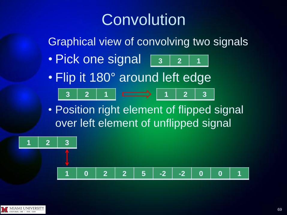
Graphical view of convolving two signals
• Pick one signal
• Flip it 180° around left edge
• Position right element of flipped signal
over left element of unflipped signal
1 0 2 2 5 -2 -2 0 0 1
3 2 1 1 2 3
3 2 1
1 2 3

Convolution
70
Graphical view
• Multiply corresponding elements and sum
3
3∙1
x
1 2 3
1 0 2 2 5 -2 -2 0 0 1
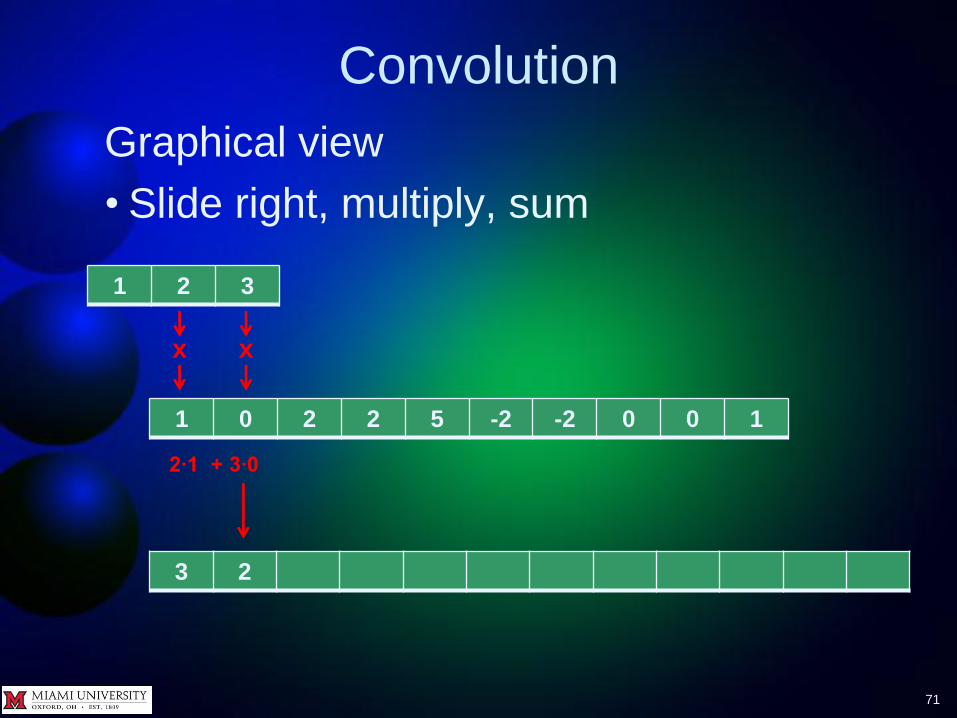
Convolution
71
Graphical view
• Slide right, multiply, sum
3 2
2∙1 + 3∙0
x
1 2 3
x
1 0 2 2 5 -2 -2 0 0 1

Convolution
72
Graphical view
• Repeat until “fall off” right side
3 2 7
1∙1 + 2∙0 + 3∙2
x
1 2 3
x x
1 0 2 2 5 -2 -2 0 0 1

Convolution
73
Graphical view
3 2 7 10
1∙0 + 2∙2 + 3∙2
x
1 2 3
x x
1 0 2 2 5 -2 -2 0 0 1
Convolution
74
Graphical view
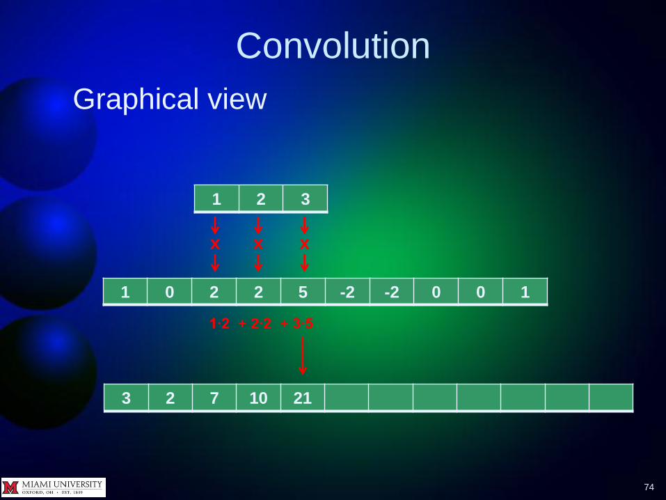
3 2 7 10 21
1∙2 + 2∙2 + 3∙5
x
1 2 3
x x
1 0 2 2 5 -2 -2 0 0 1
Convolution
75
Graphical view
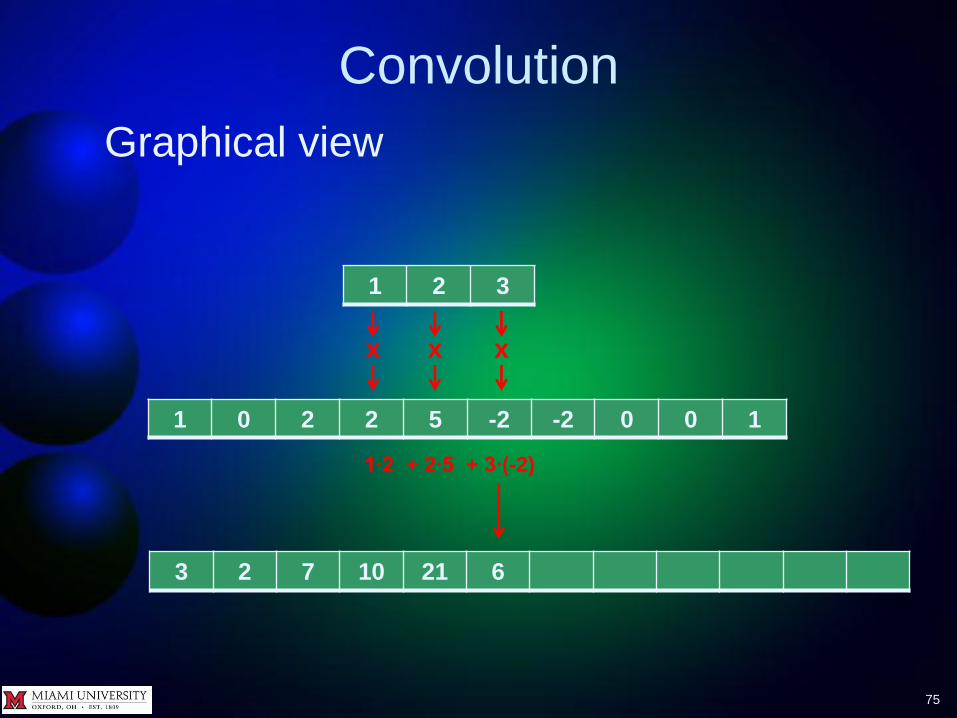
3 2 7 10 21 6
1∙2 + 2∙5 + 3∙(-2)
x
1 2 3
x x
1 0 2 2 5 -2 -2 0 0 1

Convolution
76
Graphical view
3 2 7 10 21 6 -5
1∙5 + 2∙(-2) + 3∙(-2)
x
1 2 3
x x
1 0 2 2 5 -2 -2 0 0 1
Convolution
77
Graphical view
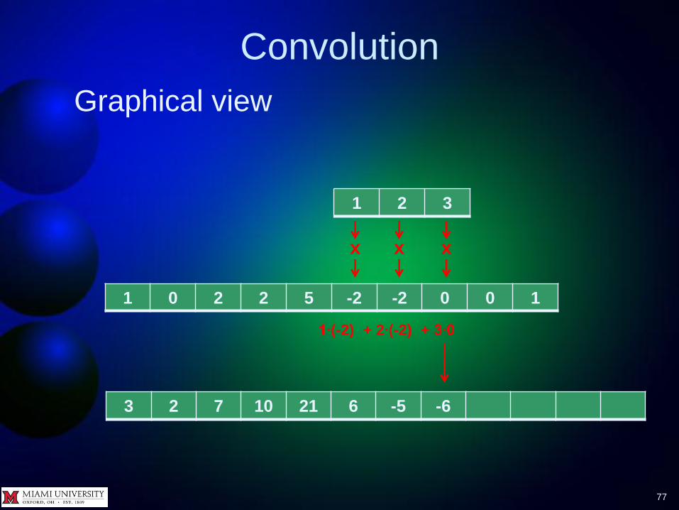
3 2 7 10 21 6 -5 -6
1∙(-2) + 2∙(-2) + 3∙0
x
1 2 3
x x
1 0 2 2 5 -2 -2 0 0 1
Convolution
78
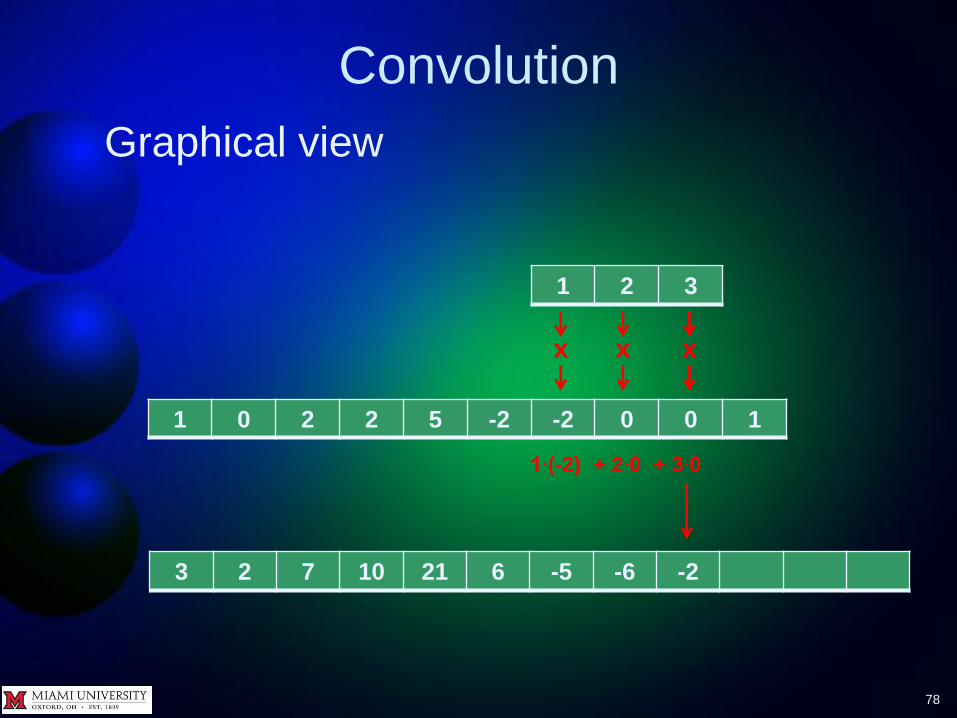
Graphical view
3 2 7 10 21 6 -5 -6 -2
1∙(-2) + 2∙0 + 3∙0
x
1 2 3
x x
1 0 2 2 5 -2 -2 0 0 1

Convolution
79
Graphical view
3 2 7 10 21 6 -5 -6 -2 3
1∙0 + 2∙0 + 3∙1
x
1 2 3
x x
1 0 2 2 5 -2 -2 0 0 1
Convolution
80
Graphical view
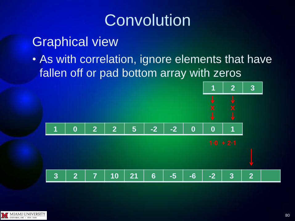
• As with correlation, ignore elements that have
fallen off or pad bottom array with zeros
3 2 7 10 21 6 -5 -6 -2 3 2
1∙0 + 2∙1
x
1 2 3
x
1 0 2 2 5 -2 -2 0 0 1

Convolution
81
Graphical view
3 2 7 10 21 6 -5 -6 -2 3 2 1
1∙1
1 2 3
x
1 0 2 2 5 -2 -2 0 0 1

Convolution
82
So convolution of
with
gives
3 2 7 10 21 6 -5 -6 -2 3 2 1
3 2 1
1 0 2 2 5 -2 -2 0 0 1

Convolution
83
Note that when we convolved with
the shorter
signal was not completely on top of the longer
one for the first two and last two elements of the
longer. For these cases, the multiply-and-add
convolution computation was missing either one
or two terms, so those four calculations are not
valid and should be ignored. Bad values at the
left and right of a convolution are known as edge
effects.
3 2 1
1 0 2 2 5 -2 -2 0 0 1

Convolution
84
In general, if the shorter of two signals
in a convolution has M elements, you
should ignore the first and last M-1
elements in the result

Convolution
85
Mathematical definition
Suppose we have two signals – x[n] has M
points and y[n] has N points, M ≤ N. The
convolution of x[n] and y[n] is
𝑤 𝑛 =
𝑥 𝑛 − 𝑘 𝑦 𝑘 for 𝑛 = 0,1,2, …𝑀 − 1
𝑛
𝑘=0
𝑥 𝑛 − 𝑘 𝑦[𝑘]
𝑛
𝑘=𝑛−𝑀+1
for 𝑛 = 𝑀,𝑀 + 1,…𝑁 − 1
𝑥 𝑛 − 𝑘 𝑦 𝑘 for 𝑛 = 𝑁,𝑁 + 1,…𝑁 + 𝑀 − 2
𝑛
𝑘=𝑛−𝑀+1
n = 0, 1, 2, … N+M-2

Convolution
86
Compute a convolution in MATLAB with
w = conv( u, v )
where
u and v are vectors. The output vector w
has length length(u)+length(v)-1

Convolution
87
TRY IT
We figured out graphically that
convolved with
gave
Try it in MATLAB >> u = [ 3 2 1 ];
>> v = [ 1 0 2 2 5 -2 -2 0 0 1 ];
>> w = conv( u, v )
w = 3 2 7 10 21 6 -5 -6 -2 3 2 1
3 2 7 10 21 6 -5 -6 -2 3 2 1
3 2 1
1 0 2 2 5 -2 -2 0 0 1
Convolution
88
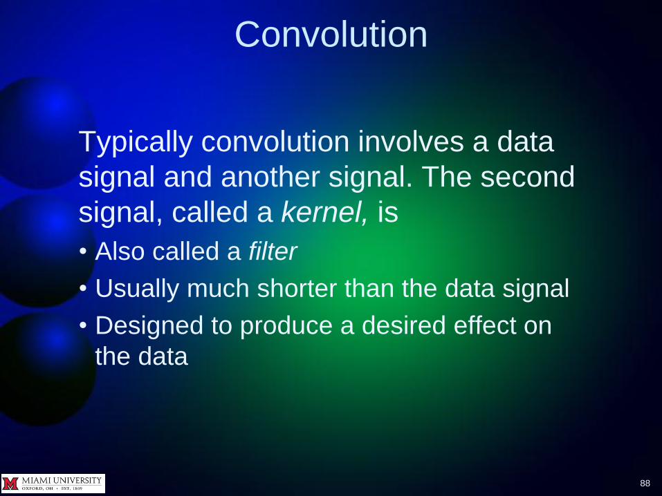
Typically convolution involves a data
signal and another signal. The second
signal, called a kernel, is
• Also called a filter
• Usually much shorter than the data signal
• Designed to produce a desired effect on
the data

Convolution
89
TRY IT
To introduce a time lag of m units
into the data signal, i.e., to shift it
to the right by m, use a kernel of m
zeros followed by a one.
Example
Introduce a lag of two into the signal
>> kernel = [ 0 0 1 ];
>> w = conv( kernel, v )
w = 0 0 1 0 2 2 5 -2 -2 0 0 1
1 0 2 2 5 -2 -2 0 0 1
Convolution
90
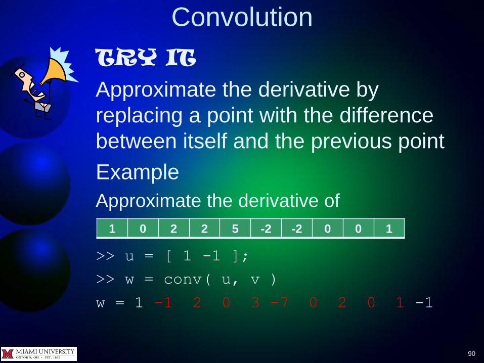
TRY IT
Approximate the derivative by
replacing a point with the difference
between itself and the previous point
Example
Approximate the derivative of
>> u = [ 1 -1 ];
>> w = conv( u, v )
w = 1 -1 2 0 3 -7 0 2 0 1 -1
1 0 2 2 5 -2 -2 0 0 1

Convolution
91
TRY IT
Reduce noise in a signal by replacing
a point with a weighted average of
itself and the previous two points
Example
>> kernel = (1/9)*[ 5 3 1 ];
>> w = conv( u, v );
w*9 = 5 3 11 16 33 7 -11 -8 -2 5 3 1
1 0 2 2 5 -2 -2 0 0 1

Convolution
92
Questions?

Signal Processing
Toolbox
93
Questions?

94
The End


