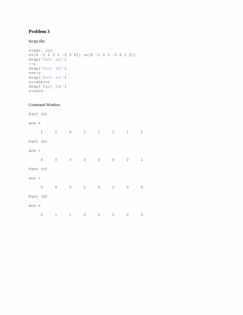
clear, clc disp('Part (a)') %alternative: sin(15*pi/180) instead of sind(15) cos(7*pi/9)+tan(7*pi/15)*sind(15) disp('Part (b)') %alternatives: could use nthroot(0.18,3), could convert to radians %and use regular trig functions sind(80)^2-(cosd(14)*sind(80))^2/(0.18)^(1/3)
clear, clc r=24; disp('Part (a)') %need to solve (a)(a/2)(a/4)=4/3 pi r^3 %could also use ^(1/3) a=nthroot(8*4/3*pi*r^3,3) disp('Part (b)') %need to solve 2(a^2/2+a^2/4+a^2/8)=4 pi r^2 a=sqrt(8/7*4*pi*r^2) disp(' ') disp('Problem 11') a=11; b=9; %could be one long expression s=sqrt(b^2+16*a^2); Labc = s/2 + b^2/(8*a)*log((4*a+s)/b)
Command Window:
Part (a) a = 77.3756 Part (b) a = 90.9520
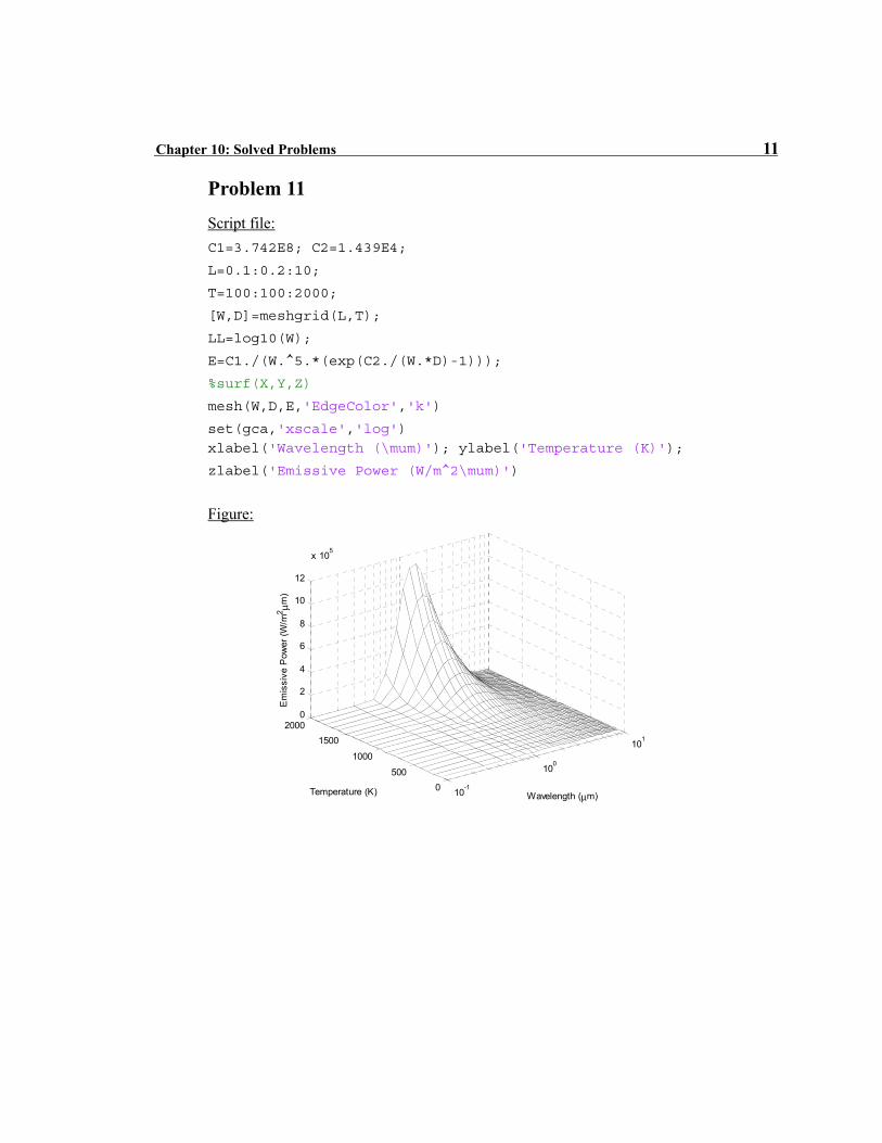
Problem 11
Script file:
clear, clc a=11; b=9; %could be one long expression s=sqrt(b^2+16*a^2); Labc = s/2 + b^2/(8*a)*log((4*a+s)/b)
clear, clc format long g variable=316501.673; %note basic matlab only has round function to nearest integer %symbolic math toolbox has round function that allows rounding to %specified digit, i.e round(variable,2) will round to 2nd digit after %the decimal point, round(variable,-3) will round to the thousands digit. disp('Part (a)') round(100*variable)/100 disp('Part (b)') round(variable/1000)*1000
clear, clc rOA=[2,5,1]; rOB=[1,3,6]; rOC=[-6,8,2]; rAC=rOC-rOA; %note, if order of rOC and rAC reversed will get negative volume Volume=dot(rOB,cross(rOC,rAC))
clear, clc T=input('Please enter the temperature in deg F: '); R=input('Please enter the relative humidity in percent: '); HI=-42.379+2.04901523*T+10.14333127*R-0.22475541*T*R-6.83783e-3*T^2 ... - 5.481717e-2*R^2+1.22874e-3*T^2*R + 8.5282e-4*T*R^2-1.99e-6*T^2*R^2; fprintf('\nThe Heat Index Temperature is: %.0f\n',HI)
Command Window:
Please enter the temperature in deg F: 90 Please enter the relative humidity in percent: 90
The Heat Index Temperature is: 122
Problem 2
Script file:
clear, clc format bank F=100000; r=4.35; years=5:10; %convert percent to decimal r=r/100; monthly_deposit=F*(r/12)./((1+r/12).^(12*years)-1); tbl=[years' monthly_deposit']; disp(' Monthly') disp(' Years Deposit') disp(tbl)
clear, clc grades=input('Please enter the grades as a vector [x x x]: '); number=length(grades); aver=mean(grades); standard_dev=std(grades); middle=median(grades); fprintf('\nThere are %i grades.\n',number) fprintf('The average grade is %.1f.\n',aver) fprintf('The standard deviation is %.1f.\n',standard_dev) fprintf('The median grade is %.1f.\n',middle)
Command Window:
Please enter the grades as a vector [x x x]: [92 74 53 61 100 42 80 66 71 78 91 85 79 68] There are 14 grades. The average grade is 74.3. The standard deviation is 15.8. The median grade is 76.0.
Problem 7
Script file:
clear, clc format short g h=4:4:40; theta=[2 2.9 3.5 4.1 4.5 5 5.4 5.7 6.1 6.4]; R=h.*cosd(theta)./(1-cosd(theta)); average=mean(R); disp('The average estimated radius of the earth in km is:') disp(average)
Command Window:
The average estimated radius of the earth in km is: 6363.1
ratio = Columns 1 through 7 1.0000 0.8118 0.6591 0.5350 0.4344 0.3526 0.2863 Columns 8 through 13 0.2324 0.1887 0.1532 0.1244 0.1010 0.0820
Problem 9
Script file:
clear, clc L=input('Please enter the mortgage amount: '); N=input('Please enter the number of years: '); r=input('Please enter the interest rate in percent: '); P=L*(r/1200)*(1+r/1200)^(12*N)/((1+r/1200)^(12*N)-1); fprintf('\nThe monthly payment of a %i years %.2f mortgage\n',N,L) fprintf('with interest rate of %.2f percent is $%.2f\n',r,P)
Command Window:
Please enter the mortgage amount: 250000 Please enter the number of years: 30 Please enter the interest rate in percent: 4.5 The monthly payment of a 30 years 250000.00 mortgage with interest rate of 4.50 percent is $1266.71
Problem 10
Script file:
clear, clc format bank A=20000; r=6.5; P=391.32; month=6:6:60; B=A*(1+r/1200).^month-P*1200/r*((1+r/1200).^month-1); perc=100*B/A; tbl=[month' B' perc']; disp(' Balance Remaining') disp(' Month $ %') disp(tbl)
clear, clc H=70; h=900; x=50:.5:1500; theta=atan(h./x)-atan((h-H)./x); [max_th indx]=max(theta); disp('The best target view occurs at a distance in feet of') disp(x(indx))
Command Window:
The best target view occurs at a distance in feet of 864.5000
Discussion: The minimum time is 59.29 seconds with the lifeguard entering the water at 37 m. Snell’s law seems only approximately satisfied, but this is due to the relatively large increment in y. The ratio converges to Snell’s law as the increment decreases. For example, decreasing the increment to .01 gives a sine ratio of 2.9996.
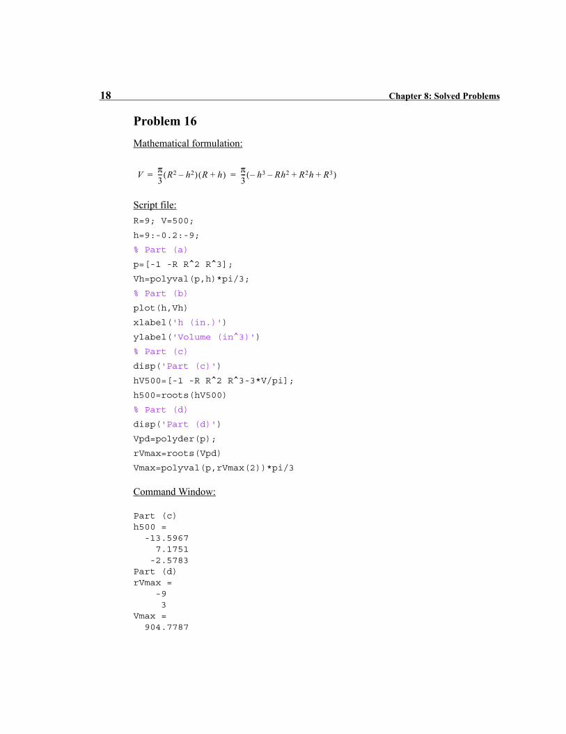
Problem 16
Script file:
clear, clc load stress_data.txt M=stress_data(1); b=stress_data(2); t=stress_data(3); a=stress_data(4); alpha=a/b; beta=pi*alpha/2; C=sqrt(tan(beta)/beta)*((0.923+0.199*(1-sin(beta))^2)/cos(beta)); sigma=6*M/(t*b^2); K=C*sigma*sqrt(pi*a); fprintf('The stress intensity factor for a beam that is %.2f m wide',b) fprintf(' and %.2f m thick\nwith an edge crack of %.2f m and an',t,a) fprintf(' applied moment of %.0f is %.0f pa-sqrt(m).\n',M,K)
Text File (stress_data.txt):
20 .25 .01 .05
Command Window:
The stress intensity factor for a beam that is 0.25 m wide and 0.01 m thick with an edge crack of 0.05 m and an applied moment of 20 is 82836 pa-sqrt(m).
Problem 17
Script file:
clear, clc v=50; rho=2000; h=500; t_90=pi*rho/(2*v); t=linspace(0,t_90,15); alpha=v*t/rho; r=sqrt(rho^2 + (h+rho)^2 - 2*rho*(rho+h)*cos(alpha)); theta=90-asind(rho*sin(alpha)./r); fprintf('For a plane flying at a speed of %.0f m/s in a circular path ',v) fprintf('of radius %.0f m\ncentered above the tracking station and ',rho) fprintf('%.0f m above the station at its lowest point:\n\n',h) %fprintf accesses elements column by column %can also use disp as shown in problem 11 tbl=[t;theta;r]; fprintf(' Time Tracking Distance\n') fprintf(' (s) Angle (deg) (m)\n') fprintf(' %4.1f %4.1f %6.1f\n',tbl)
Command Window:
For a plane flying at a speed of 50 m/s in a circular path of radius 2000 m centered above the tracking station and 500 m above the station at its lowest point: Time Tracking Distance (s) Angle (deg) (m) 0.0 90.0 500.0 4.5 66.4 559.4 9.0 51.0 707.6 13.5 42.8 900.6 18.0 38.8 1113.7 22.4 37.2 1335.2 26.9 36.9 1559.4 31.4 37.5 1783.0 35.9 38.7 2003.8 40.4 40.3 2220.3 44.9 42.2 2431.3 49.4 44.3 2635.8 53.9 46.5 2832.8 58.3 48.9 3021.6 62.8 51.3 3201.6
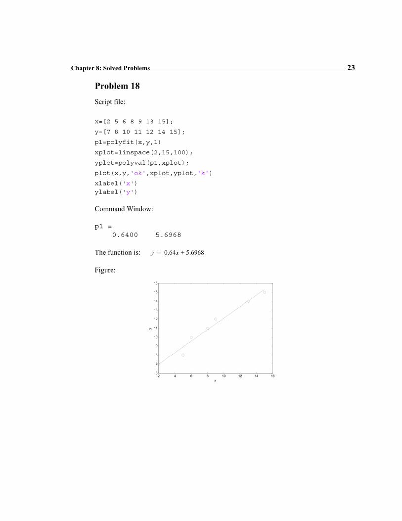
Problem 18
Script file:
clear, clc C=13.83; Eg=0.67; k=8.62e-5; T=xlsread('Germanium_data.xlsx'); sigma=exp(C-Eg./(2*k*T)); tbl=[T sigma]; disp(' Intrinsic') disp(' Temperature Conductivity') disp(' deg K (ohm-m)^-1') %can also use disp as shown in problem 11 fprintf(' %4.0f %5.1f\n',tbl')
Command Window: Excel File:
Intrinsic Temperature Conductivity deg K (ohm-m)^-1 400 61.2 435 133.7 475 283.8 500 427.3 520 576.1 545 811.7
Problem 19
Script file:
clear, clc rho=input('Please input the fluid density in kg/m^3: '); v=input('Please input the fluid velocity in m/s: '); d_ratio=input('Please input the pipe diameter ratio as a vector [x x x]: '); delP=0.5*(1-d_ratio.^2).^2*rho*v^2; fprintf('\nFor gasoline with a density of %.0f kg/m^3 and a flow ',rho) fprintf('velocity of %.1f m/s\n\n',v) tbl=[d_ratio;delP]; disp(' delta P') disp(' d/D (Pa)') fprintf(' %3.1f %6.1f\n',tbl)
Command Window:
Please input the fluid density in kg/m^3: 737 Please input the fluid velocity in m/s: 5 Please input the pipe diameter ratio as a vector [x x x]: [.9:-.1:.4 .2] For gasoline with a density of 737 kg/m^3 and a flow velocity of 5.0 m/s delta P d/D (Pa) 0.9 332.6 0.8 1193.9 0.7 2396.2 0.6 3773.4 0.5 5182.0 0.4 6500.3 0.2 8490.2
Problem 20
Script file:
clear, clc sigma=5.669e-8; T1=input('Please input the temperature of plate 1 in deg K: '); T2=input('Please input the temperature of plate 2 in deg K: '); a=input('Please input the radius of plate 1 in m: '); b=input('Please input the radius of plate 2 in m: '); c=input('Please input the distance between plate 1 and plate 2 in m: '); X=a./c; Y=c/b; Z=1+(1+X.^2).*Y.^2; F_1_2 = 0.5*(Z-sqrt(Z.^2-4*X.^2.*Y.^2)); q=sigma*pi*b^2*F_1_2*(T1^4-T2^4); fprintf('\nFor circular plate 1 with radius %i m and temperature %i',a,T1) fprintf(' deg K\nand circular plate 2 with radius %i m and temperature',b) fprintf(' %i deg K\n',T2) tbl=[c;q]; fprintf('\n Radiation\n') fprintf(' Separation Heat Exchange\n') fprintf(' (m) (Watts)\n') fprintf(' %4.1f %6.0f\n',tbl)
Command Window:
Please input the temperature of plate 1 in deg K: 400 Please input the temperature of plate 2 in deg K: 600 Please input the radius of plate 1 in m: 1 Please input the radius of plate 2 in m: 2 Please input the distance between plate 1 and plate 2 in m: 10.^(-1:1) For circular plate 1 with radius 1 m and temperature 400 deg K and circular plate 2 with radius 2 m and temperature 600 deg K Radiation Separation Heat Exchange (m) (Watts) 0.1 -18461 1.0 -14150 10.0 -706
Problem 21
Script file:
clear, clc x1=input('Please enter the coordinates of point 1 as a vector [x x]: '); x2=input('Please enter the coordinates of point 2 as a vector [x x]: '); x3=input('Please enter the coordinates of point 3 as a vector [x x]: '); A=2*[x1(1)-x2(1) x1(2)-x2(2); x2(1)-x3(1) x2(2)-x3(2)]; B=[x1(1)^2+x1(2)^2-x2(1)^2-x2(2)^2; x2(1)^2+x2(2)^2-x3(1)^2-x3(2)^2]; C=A\B; r=sqrt((x1(1)-C(1))^2 + (x1(2)-C(2))^2); fprintf('\nThe coordinates of the center are (%.1f, %.1f) ',C) fprintf('and the radius is %.1f.\n',r)
Command Window:
Please enter the coordinates of point 1 as a vector [x x]: [10.5, 4] Please enter the coordinates of point 2 as a vector [x x]: [2, 8.6] Please enter the coordinates of point 3 as a vector [x x]: [-4, -7] The coordinates of the center are (2.5, -0.6) and the radius is 9.2.
clear, clc %.1 is usually a good interval to start with - then adjust if necessary x=-1:.1:5; f=(x.^2-3*x+7)./sqrt(2*x+5); plot(x,f) %note all plot annotation functions will accept some basic tex syntax title('f(x)=(x^2-3x+7)/sqrt(2x+5)') %and latex commands for fancier %title('$$f(x)=\frac{x^2-3x+7}{\sqrt{2x+5}}$$','Interpreter','latex') xlabel('x-->') ylabel('f(x)-->')
The linear plot is useful for telling when the level of contraction becomes significant. The log-log plot is useful because the relationship is almost linear when plotted this way.
clear n=input('Please enter the size of the Pascal matrix to be created: '); for i=1:n for j=1:n A(i,j)=factorial(i+j-2)/(factorial(i-1)*factorial(j-1)); end end A
Command Window:
Please enter the size of the Pascal matrix to be created: 4 A = 1 1 1 1 1 2 3 4 1 3 6 10 1 4 10 20 >> PascalMatrix Please enter the size of the Pascal matrix to be created: 7 A = 1 1 1 1 1 1 1 1 2 3 4 5 6 7 1 3 6 10 15 21 28 1 4 10 20 35 56 84 1 5 15 35 70 126 210 1 6 21 56 126 252 462 1 7 28 84 210 462 924
Problem 8
Script file:
clear, clc BOS=[2.67 1.00 1.21 3.09 3.43 4.71 3.88 3.08 4.10 2.62 1.01 5.93]; SEA=[6.83 3.63 7.20 2.68 2.05 2.96 1.04 0.00 0.03 6.71 8.28 6.85]; disp('Part (a)') B_T=sum(BOS); B_A=mean(BOS); S_T=sum(SEA); S_A=mean(SEA); fprintf('The total precipitation in Boston in 2012 was %.2f in',B_T) fprintf(' and average %.2f in\n',B_A) fprintf('The total precipitation in Seattle in 2012 was %.2f in',S_T) fprintf(' and average %.2f in\n\n',S_A) disp('Part (b)') B_D=sum(BOS>B_A); S_D=sum(SEA>S_A); fprintf('Boston had %i months above average and Seattle %i months\n\n',B_D,S_D) disp('Part (c)') BltS=sum(BOS<SEA); m=1:12; fprintf('The precipitation was lower in Boston in the following %i months:',BltS) fprintf(' %i',m(BOS<SEA)) fprintf('\n')
Command Window:
Part (a) The total precipitation in Boston in 2012 was 36.73 in and average 3.06 in The total precipitation in Seattle in 2012 was 48.26 in and average 4.02 in Part (b) Boston had 7 months above average and Seattle 5 months Part (c) The precipitation was lower in Boston in the following 6 months: 1 2 3 10 11 12
Problem 9
Script file:
clear, clc i=0; s=0; while s<=120 i=i+1; if rem(i,2)==0 && rem(i,13)==0 && rem(i,16)==0 s=sqrt(i); end end fprintf('The required number is: %i\n',i)
Command Window:
The required number is: 14560
Problem 10
Script file:
clear, clc f(1)=0; f(2)=1; for k=1:18 f(k+2)=f(k)+f(k+1); end fprintf('The first 20 Fibonacci numbers are:\n') fprintf(' %i',f) fprintf('\n')
clear, clc n=[10 50 100]; f(1)=1; f(2)=1; for j=1:3 S=2; for k=3:n(j) f(k)=f(k-1)+f(k-2); S=S+1/f(k); end fprintf('The sum after %i terms is: %.12f\n',n(j),S) end
Command Window:
The sum after 10 terms is: 3.330469040763 The sum after 50 terms is: 3.359885666115 The sum after 100 terms is: 3.359885666243
Problem 12
Script file:
clear, clc for k=1:3 disp('For the equation ax^2+bx+c') a=input('Enter a: '); b=input('Enter b: '); c=input('Enter c: '); D=b^2-4*a*c; if D<0 fprintf('\nThe equation has no real roots.\n\n') elseif D==0 root=-b/(2*a); fprintf('\nThe equation has one root,\n') fprintf(' %.3f\n\n',root) else r1=(-b+sqrt(D))/(2*a); r2=(-b-sqrt(D))/(2*a); fprintf('\nThe equation has two roots,\n') fprintf(' %.3f and %.3f\n\n',r1,r2) end end
Command Window:
For the equation ax^2+bx+c Enter a: 3 Enter b: 6 Enter c: 3 The equation has one root, -1.000 For the equation ax^2+bx+c Enter a: -3 Enter b: 4 Enter c: -6 The equation has no real roots. For the equation ax^2+bx+c Enter a: -3 Enter b: 7 Enter c: 5 The equation has two roots, -0.573 and 2.907
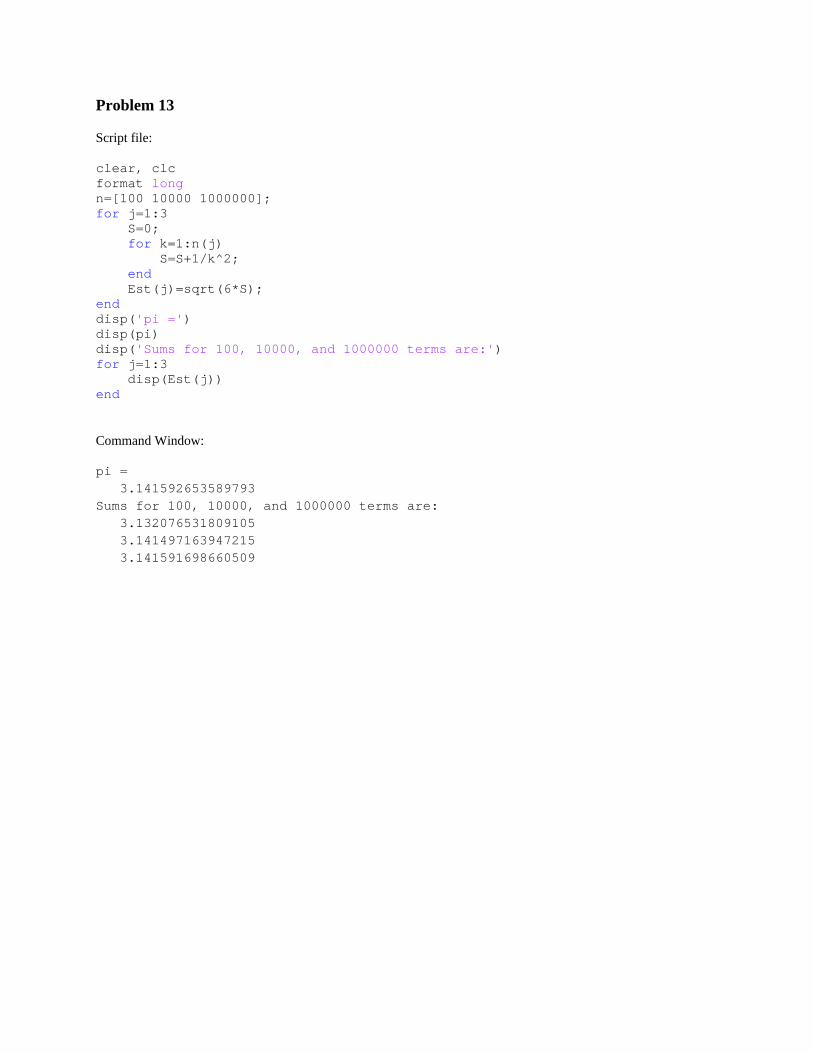
Problem 13
Script file:
clear, clc format long n=[100 10000 1000000]; for j=1:3 S=0; for k=1:n(j) S=S+1/k^2; end Est(j)=sqrt(6*S); end disp('pi =') disp(pi) disp('Sums for 100, 10000, and 1000000 terms are:') for j=1:3 disp(Est(j)) end
Command Window:
pi = 3.141592653589793 Sums for 100, 10000, and 1000000 terms are: 3.132076531809105 3.141497163947215 3.141591698660509
Problem 14
Script file:
clear, clc format long n=[5 10 40]; for j=1:3 t(1)=sqrt(2)/2; T=t(1); for k=2:n(j) t(k)=sqrt(2+2*t(k-1))/2; T=T*t(k); end Est(j)=2/T; end disp('pi =') disp(pi) disp('Results for 5, 10, and 40 terms are:') for j=1:3 disp(Est(j)) end
Command Window:
pi = 3.141592653589793 Results for 5, 10, and 40 terms are: 3.140331156954753 3.141591421511200 3.141592653589794
Problem 15
Script file:
clear, clc vector=20*rand(1,20)-10; S=0; for k=1:20 if(vector(k)>0) S=S+vector(k); end end disp('The sum of the positive elements is: ') disp(S)
Command Window:
The sum of the positive elements is:
52.5755
Problem 16
Script file:
clear, clc vector=randi(20,1,20)-10; iter=0; N=-1; while N<0 N=1; for k=1:20 if vector(k)<0 N=-1; vector(k)=randi(20)-10; end end if N == -1 iter=iter+1; end end vector disp('The number of iterations needed to make all elements of vector positive') disp(iter)
Command Window:
vector =
3 4 5 6 1 2 5 2 4 7 7 5 8 0 2 6 5 0 4 9
The number of iterations needed to make all elements of vector positive
4
Problem 17
Script file:
vector=input('Please enter any array of integers of any length: ') n=0; np=0; nn3=0; for k=1:length(vector) n=n+1; if vector(k)>0 np=np+1; elseif vector(k)<0 & rem(vector(k),3)==0 nn3=nn3+1; end end fprintf('The vector has %i elements. %i elements are positive\n',n,np) fprintf('and %i elements are negative divisible by 3\n',nn3)
Command Window:
Please enter any array of integers of any length: randi([-20 20],1,16) vector = 15 -16 17 -16 1 -15 2 -20 11 14 17 20 0 -9 -16 0 The vector has 16 elements. 8 elements are positive and 2 elements are negative divisible by 3
Problem 18
Script file:
clear, clc x=[4.5 5 -16.12 21.8 10.1 10 -16.11 5 14 -3 3 2]; for k=1:length(x)-1 for j=k+1:length(x) if x(j)<x(k) temp=x(k); x(k)=x(j); x(j)=temp; end end end x
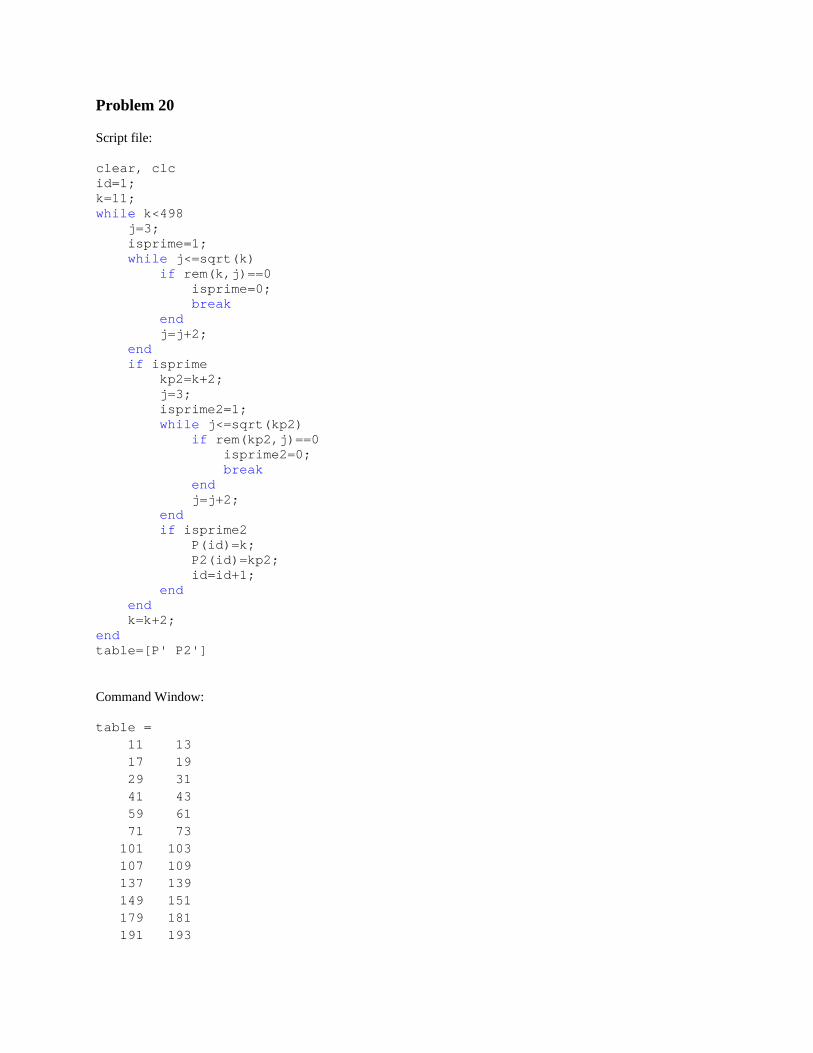
clear, clc id=1; k=11; while k<498 j=3; isprime=1; while j<=sqrt(k) if rem(k,j)==0 isprime=0; break end j=j+2; end if isprime kp2=k+2; j=3; isprime2=1; while j<=sqrt(kp2) if rem(kp2,j)==0 isprime2=0; break end j=j+2; end if isprime2 P(id)=k; P2(id)=kp2; id=id+1; end end k=k+2; end table=[P' P2']
clear, clc id=1; for k=49:2:101 j=3; isprime=1; while j<=sqrt(k) if rem(k,j)==0 isprime=0; break end j=j+2; end if isprime P(id)=k; id=id+1; end end id=1; for k=2:length(P)-1 if P(k+1)~=P(k)+2 & P(k-1)~=P(k)-2 iso(id)=P(k); id=id+1; end end disp('The isolated primes between 50 and 100 are:') disp(iso)
Command Window:
The isolated primes between 50 and 100 are:
67 79 83 89 97
Problem 22
Script file:
scores=[31 70 92 5 47 88 81 73 51 76 80 90 55 23 43 98 36 ... 87 22 61 19 69 26 82 89 99 71 59 49 64]; n(1:5)=0; for k=1:length(scores) if scores(k)<20 n(1)=n(1)+1; elseif scores(k)<40 n(2)=n(2)+1; elseif scores(k)<60 n(3)=n(3)+1; elseif scores(k)<80 n(4)=n(4)+1; else n(5)=n(5)+1; end end fprintf('Grades between 0 and 19 %3i students\n',n(1)) fprintf('Grades between 20 and 39 %3i students\n',n(2)) fprintf('Grades between 40 and 59 %3i students\n',n(3)) fprintf('Grades between 60 and 79 %3i students\n',n(4)) fprintf('Grades between 80 and 100 %3i students\n',n(5))
Command Window:
Grades between 0 and 19 2 students Grades between 20 and 39 5 students Grades between 40 and 59 6 students Grades between 60 and 79 7 students Grades between 80 and 100 10 students
Problem 23 Script file:
clear, clc for j=1:2 angle=input('Please input an angle in degrees: '); x=angle*pi/180; E=1; S=0; k=0; while E>.000001 S_old=S; S=S+(-1)^k/factorial(2*k)*x^(2*k); E=abs((S-S_old)/S_old); k=k+1; end fprintf('\nThe value of cosine of %.0f degrees is %.8f\n\n',angle,S) end
Command Window:
Please input an angle in degrees: 35 The value of cosine of 35 degrees is 0.81915205 Please input an angle in degrees: 125 The value of cosine of 125 degrees is -0.57357644
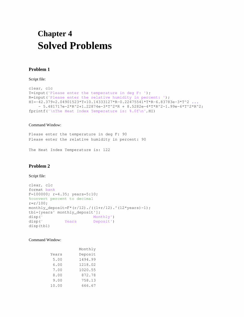
Problem 24
Script file:
clear, clc k=1; S=1; while S<1000 S=k*(k+1)/2; d1=floor(S/100); d2=floor((S-d1*100)/10); d3=floor(S-d1*100-d2*10); if d1==d2 & d2==d3 break end k=k+1; end fprintf('The desired sum is %i\n', S) fprintf('This is the sum of the first %i digits\n',k)
Command Window:
The desired sum is 666
This is the sum of the first 36 digits
Problem 25
Script file:
clear, clc for k=1:2 gender=input('Please input your gender (male or female): ','s'); age=input('Please input your age: '); RHR=input('Please enter your resting heart rate: '); fit=input('Please enter your fitness level (low, medium, or high: ','s'); gender = lower(gender); fit = lower(fit); switch fit case 'low' INTEN=0.55; case 'medium' INTEN=0.65; case 'high' INTEN=0.8; end switch gender case 'male' THR=((220-age)-RHR)*INTEN+RHR; case 'female' THR=((206-0.88*age)-RHR)*INTEN+RHR; end fprintf('\nThe recommended training heart rate is %.0f\n\n',THR) end
Command Window:
Please input your gender (male or female): male Please input your age: 21 Please enter your resting heart rate: 62 Please enter your fitness level (low, medium, or high: low The recommended training heart rate is 137 Please input your gender (male or female): female Please input your age: 19 Please enter your resting heart rate: 67 Please enter your fitness level (low, medium, or high: high The recommended training heart rate is 165
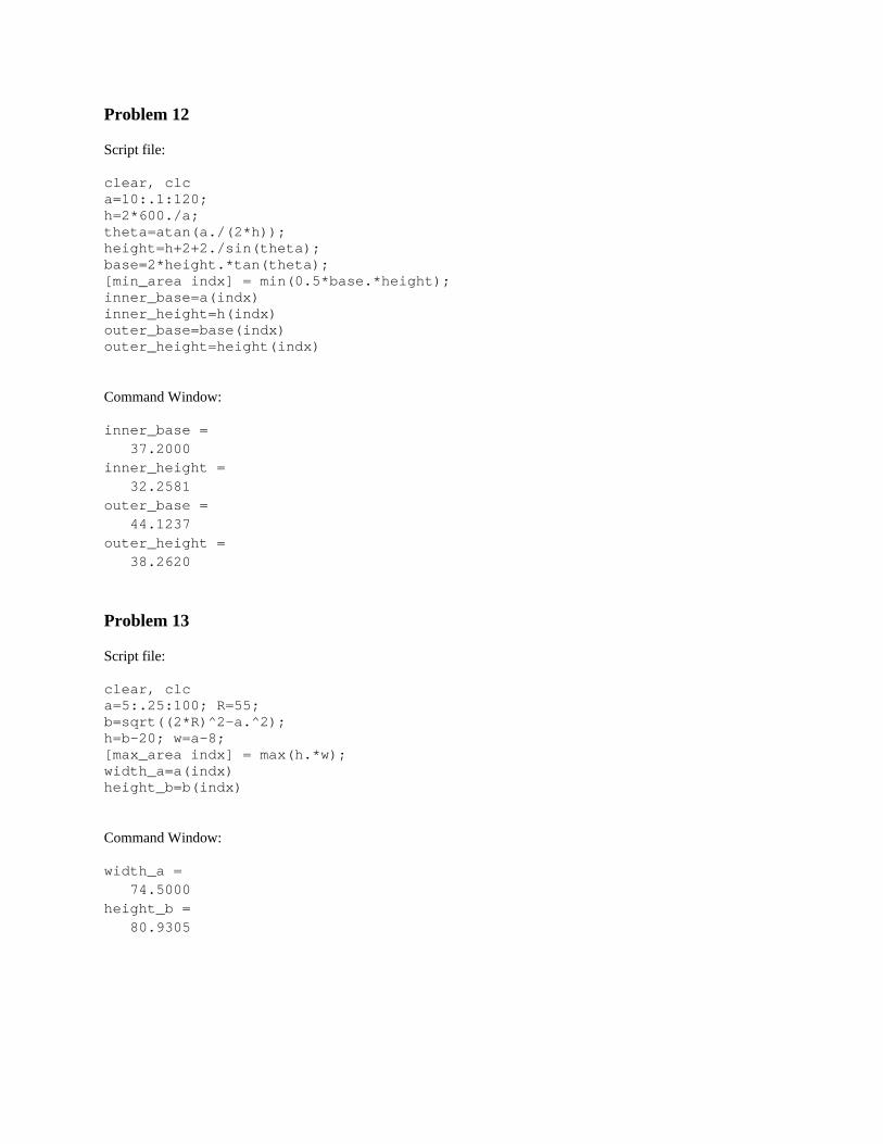
Problem 26
Script file:
clear, clc for j=1:2 W=input('Please input your weight in lb: '); h=input('Please input your height in in: '); BMI=703*W/h^2; if BMI<18.5 fprintf('\nYour BMI value is %.1f, which classifies you as underweight\n\n',BMI) elseif BMI<25 fprintf('\nYour BMI value is %.1f, which classifies you as normal\n\n',BMI) elseif BMI<30 fprintf('\nYour BMI value is %.1f, which classifies you as overweight\n\n',BMI) else fprintf('\nYour BMI value is %.1f, which classifies you as obese\n\n',BMI) end end
Command Window:
Please input your weight in lb: 180 Please input your height in in: 74 Your BMI value is 23.1, which classifies you as normal Please input your weight in lb: 150 Please input your height in in: 61 Your BMI value is 28.3, which classifies you as overweight
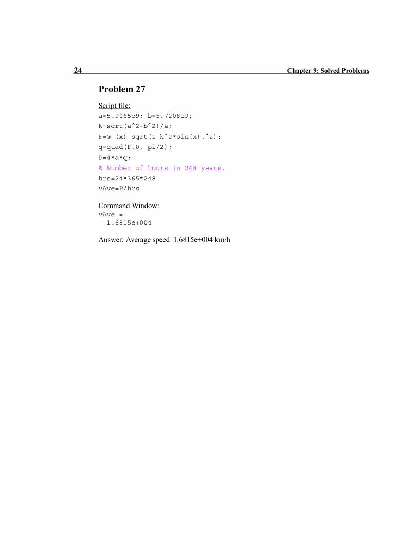
Problem 27
Script file:
clear, clc for j=1:3 service=input('Please input the type of service\n G for Ground, E for Express, O for Overnight: ','s'); wt=input('Please enter the weight of the package as [lb oz]: '); service = lower(service); wgt=wt(1)+wt(2)/16; switch service case 'g' if wgt<0.5 cost=.7+.06*wt(2); elseif wgt<5 u=ceil(2*(wgt-0.5)); cost=1.18+.42*u; else cost=4.96+.72*ceil(wgt-5); end case 'e' if wgt<0.5 cost=2.4+.25*wt(2); elseif wgt<5 u=ceil(2*(wgt-0.5)); cost=4.40+1.2*u; else cost=15.2+1.8*ceil(wgt-5); end case 'o' if wgt<0.5 cost=12.20+.8*wt(2); elseif wgt<5 u=ceil(2*(wgt-0.5)); cost=18.6+4.8*u; else cost=61.8+6.4*ceil(wgt-5); end end fprintf('\nThe cost of service will be $%.2f\n\n',cost) end
Command Window:
Please input the type of service G for Ground,E for Express, O for Overnight: G Please enter the weight of the package as [lb oz]: [2 7] The cost of service will be $2.86 Please input the type of service G for Ground,E for Express, O for Overnight: E Please enter the weight of the package as [lb oz]: [0 7]
The cost of service will be $4.15 Please input the type of service G for Ground,E for Express, O for Overnight: O Please enter the weight of the package as [lb oz]: [5 10] The cost of service will be $68.20
Problem 28
Script file:
clear, clc for j=1:3 n(1:8)=0; cost=randi([1 5000],1,1)/100; fprintf('The total charge is $%.2f\n',cost) pay=input('Please enter payment (1, 5, 10, 20, or 50): '); if pay<cost fprintf('Insufficient Payment\n\n') continue else change=pay-cost; if change>=20 n(1)=1; change=change-20; end if change>=10 n(2)=1; change=change-10; end if change>=5 n(3)=1; change=change-5; end while change>=1 n(4)=n(4)+1; change=change-1; end while change>=.25 n(5)=n(5)+1; change=change-.25; end while change>=.10 n(6)=n(6)+1; change=change-.10; end if change>=.05 n(7)=1; change=change-.05; end change=change+.000001; while change>=.01 n(8)=n(8)+1; change=change-.01; end end fprintf('\n $20 $10 $5 $1 $0.25 $0.10 $0.05 $0.01\n') fprintf(' %i',n) fprintf('\n\n') end
Command Window:
The total charge is $44.39 Please enter payment (1, 5, 10, 20, or 50): 50 $20 $10 $5 $1 $0.25 $0.10 $0.05 $0.01 0 0 1 0 2 1 0 1 The total charge is $9.94 Please enter payment (1, 5, 10, 20, or 50): 50 $20 $10 $5 $1 $0.25 $0.10 $0.05 $0.01 1 1 1 5 0 0 1 1 The total charge is $19.77 Please enter payment (1, 5, 10, 20, or 50): 5 Insufficient Payment
clear, clc n=[100 53701 19.35]; for j=1:3 P=n(j); x=P; E=1; while E>.00001 x_old=x; x=(P/x^2+2*x)/3; E=abs((x-x_old)/x_old); end fprintf('The cube root of %.0f is %.1f\n',P,x) end Command Window:
The cube root of 100 is 4.6 The cube root of 53701 is 37.7 The cube root of 19 is 2.7
Problem 31 Script file:
clear, clc for j=1:3 p=input('Please enter the pressure: '); old=input('Please enter the units (Pa, psi, atm, or torr): ','s'); new=input('Please enter the desired units (Pa, psi, atm, or torr): ','s'); switch old case 'Pa' temp=p; case 'psi' temp=6.894757e03*p; case 'atm' temp=1.01325e05*p; case 'torr' temp=1.333224e02*p; end switch new case 'Pa' pnew=temp; case 'psi' pnew=temp/6.894757e03; case 'atm' pnew=temp/1.01325e05; case 'torr' pnew=temp/1.333224e02; end fprintf('The converted pressure is %.1f %s\n\n',pnew,new) end
Command Window:
Please enter the pressure: 70 Please enter the units (Pa, psi, atm, or torr): psi Please enter the desired units (Pa, psi, atm, or torr): Pa The converted pressure is 482633.0 Pa Please enter the pressure: 120 Please enter the units (Pa, psi, atm, or torr): torr Please enter the desired units (Pa, psi, atm, or torr): atm The converted pressure is 0.2 atm Please enter the pressure: 8000 Please enter the units (Pa, psi, atm, or torr): Pa Please enter the desired units (Pa, psi, atm, or torr): psi The converted pressure is 1.2 psi
Problem 32 Script file:
clear, clc for k=1:100 x=0; n(k)=0; while abs(x)<10 x=x+randn(1,1); n(k)=n(k)+1; end end fprintf('The average number of steps to reach the boundary are %.1f\n',mean(n))
Command Window:
The average number of steps to reach the boundary are 119.0
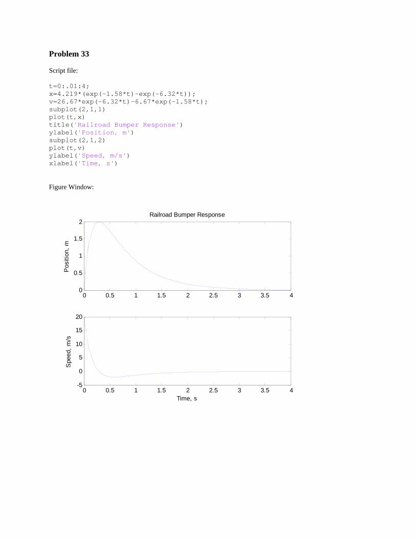
Problem 33
Script file:
n=[10 100 1000 10000]; for j=1:4 x(1)=0; y(1)=0; for k=2:n(j) m=randi([1 3],1,1); switch m case 1 x(k)=0.5*x(k-1); y(k)=0.5*y(k-1); case 2 x(k)=0.5*x(k-1)+0.25; y(k)=0.5*y(k-1)+sqrt(3)/4; case 3 x(k)=0.5*x(k-1)+0.5; y(k)=0.5*y(k-1); end end figure(j) plot(x,y,'^') end
Figure Windows:
0 0.1 0.2 0.3 0.4 0.5 0.6 0.7 0.80
0.1
0.2
0.3
0.4
0.5
0.6
0.7
0 0.1 0.2 0.3 0.4 0.5 0.6 0.7 0.8 0.9 10
0.1
0.2
0.3
0.4
0.5
0.6
0.7
0.8
0.9
0 0.1 0.2 0.3 0.4 0.5 0.6 0.7 0.8 0.9 10
0.1
0.2
0.3
0.4
0.5
0.6
0.7
0.8
0.9
0 0.1 0.2 0.3 0.4 0.5 0.6 0.7 0.8 0.9 10
0.1
0.2
0.3
0.4
0.5
0.6
0.7
0.8
0.9
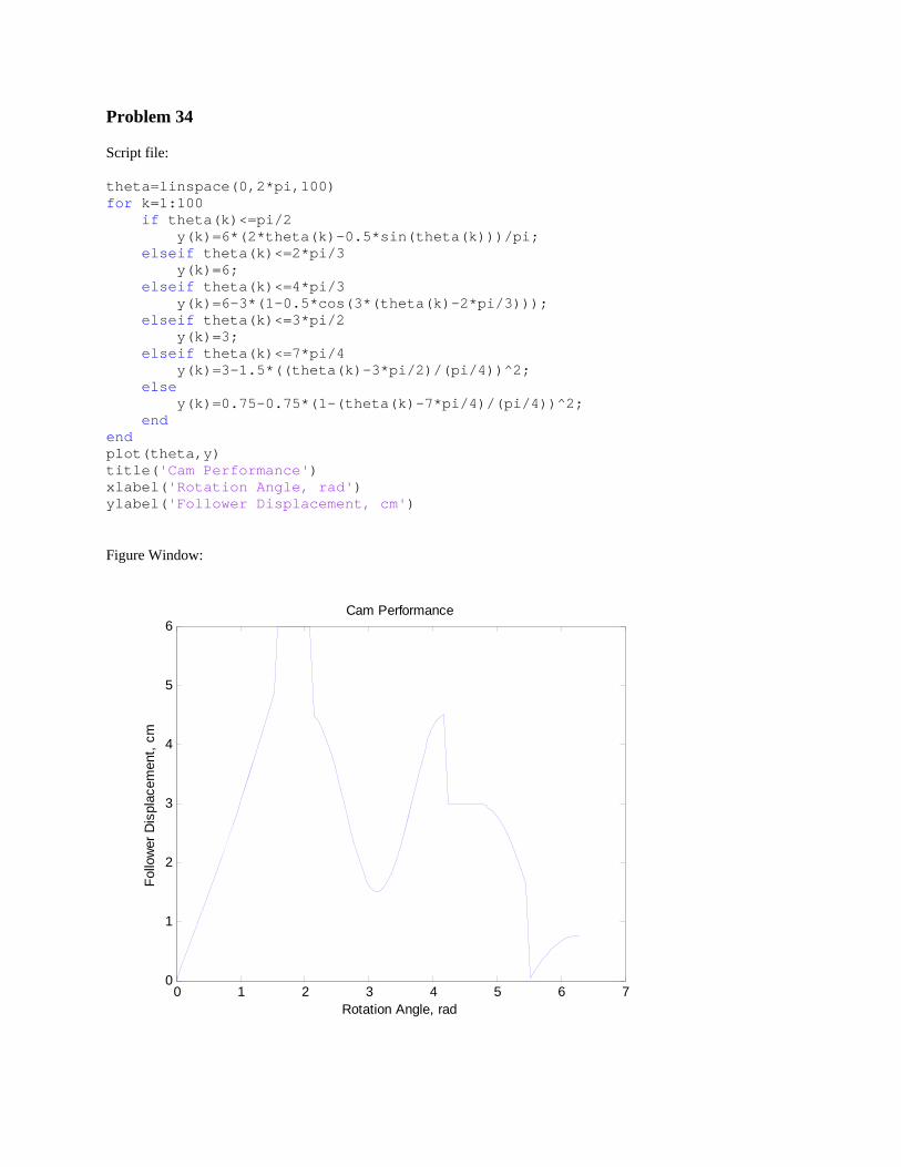
Problem 34
Script file:
theta=linspace(0,2*pi,100) for k=1:100 if theta(k)<=pi/2 y(k)=6*(2*theta(k)-0.5*sin(theta(k)))/pi; elseif theta(k)<=2*pi/3 y(k)=6; elseif theta(k)<=4*pi/3 y(k)=6-3*(1-0.5*cos(3*(theta(k)-2*pi/3))); elseif theta(k)<=3*pi/2 y(k)=3; elseif theta(k)<=7*pi/4 y(k)=3-1.5*((theta(k)-3*pi/2)/(pi/4))^2; else y(k)=0.75-0.75*(1-(theta(k)-7*pi/4)/(pi/4))^2; end end plot(theta,y) title('Cam Performance') xlabel('Rotation Angle, rad') ylabel('Follower Displacement, cm')
Figure Window:
0 1 2 3 4 5 6 70
1
2
3
4
5
6Cam Performance
Rotation Angle, rad
Follo
wer
Dis
plac
emen
t, cm
Problem 35
Script file:
clear, clc for j=1:2 quiz=input('Please enter the quiz grades as a vector [x x x x x x]: '); mid=input('Please enter the midterm grades as a vector [x x x]: '); final=input('Please enter the final exam grade: '); q_c=(sum(quiz)-min(quiz))/5; if mean(mid)>final grade=3*q_c + 0.5*mean(mid) + 0.2*final; else grade=3*q_c + 0.2*mean(mid) + 0.5*final; end if grade>=90 letter='A'; elseif grade>=80 letter='B'; elseif grade>=70 letter='C'; elseif grade>=60 letter='D'; else letter='E'; end fprintf('\nThe overall course grade is %.1f for a letter grade of %s\n\n',grade,letter) end Command Window: Please enter the quiz grades as a vector [x x x x x x]: [6 10 6 8 7 8] Please enter the midterm grades as a vector [x x x]: [82 95 89] Please enter the final exam grade: 81 The overall course grade is 83.9 for a letter grade of B Please enter the quiz grades as a vector [x x x x x x]: [9 5 8 8 7 6] Please enter the midterm grades as a vector [x x x]: [78 82 75] Please enter the final exam grade: 81 The overall course grade is 79.0 for a letter grade of C
Problem 36 Script file:
clear, clc for j=1:2 disp(' ') mat=input('Please enter the golfer''s rounds as a table: '); [n,m]=size(mat); hcp=113*(mat(:,3)-mat(:,1))./mat(:,2); if n>=20 N=10; elseif n==19 N=9; elseif n==18 N=8; elseif n==17 N=7; elseif n>=15 N=6; elseif n>=13 N=5; elseif n>=11 N=4; elseif n>=9 N=3; elseif n>=7 N=2; else N=1; end for k=1:n-N [mval id]=max(hcp); hcp(id)=[]; end Players_handicap=floor(10*mean(hcp))/10 end Command Window:
clear, clc disp('Part (a)') x=[-1.5 5]; y=math(x); disp('The test values for y(x) are:') disp(y) % %part b x=-2:.1:6; plot(x,math(x)); title('y(x)=(-0.2x^3 + 7x^2)e^{-0.3x}') xlabel('x-->') ylabel('y-->')
Function file:
function y = math(x) y=(-0.2*x.^3+7*x.^2).*exp(-0.3*x);
Command Window: Figure Window: Part (a) The test values for y(x) are: 25.7595 33.4695
-2 -1 0 1 2 3 4 5 60
10
20
30
40
50
60y(x)=(-0.2x3 + 7x2)e-0.3x
x-->
y-->
Problem 2
Script file:
clear, clc disp('Part (a)') th=[pi/6, 5*pi/6]; r=polarmath(th); disp('The test values for r(theta) are:') disp(r) % %part b th=linspace(0,2*pi,200); polar(th,polarmath(th)); title('r(\theta)=4cos(4sin(\theta))') Function file:
function r = polarmath(theta) %angles in radians r=4*cos(4*sin(theta)); Command Window:
Part (a) The test values for r(theta) are: -1.6646 -1.6646 1 Figure Window:
1
2
3
4
30
210
60
240
90
270
120
300
150
330
180 0
r(θ)=4cos(4sin(θ))
Problem 3
Script file:
clear, clc disp('Part (a)') gmi=5; Lkm = LkmToGalm(gmi); disp('The fuel consumption of a Boeing 747 in liters/km is:') disp(Lkm) disp('Part (b)') gmi=5.8; Lkm = LkmToGalm(gmi); disp('The fuel consumption of a Concorde in liters/km is:') disp(Lkm) Function file:
function Lkm = LkmToGalm(gmi) Lkm = gmi*4.40488/1.609347; Command Window:
Part (a) The fuel consumption of a Boeing 747 in liters/km is: 13.6853 Part (b) The fuel consumption of a Concorde in liters/km is: 15.8750
Problem 4
Script file:
clear, clc disp('Part (a)') den=7860; sw = DenTOSw(den); disp('The specific weight of steel in lb/in^3 is:') disp(sw) disp('Part (b)') den=4730; sw = DenTOSw(den); disp('The specific weight of titanium in lb/in^3 is:') disp(sw) Function file:
function sw = DenTOSw(den) sw=den/2.76799e4;
Command Window:
Part (a) The specific weight of steel in lb/in^3 is: 0.2840 Part (b) The specific weight of titanium in lb/in^3 is: 0.1709
Problem 5
Script file:
kts=400; fps = ktsTOfps(kts); fprintf('A speed of 400 kts is %.1f ft/s\n',fps) Function file:
function fps = ktsTOfps(kts) fps=kts*6076.1/3600; Command Window:
A speed of 400 kts is 675.1 ft/s
Problem 6
Script file:
clear, clc disp('Part (a)') w=95; h=1.87; BSA = BodySurA(w,h); fprintf('The body surface area of a %.0f kg, %.2f m patient is %.3f m^2\n',w,h,BSA) disp('Part (b)') w=61; h=1.58; BSA = BodySurA(w,h); fprintf('The body surface area of a %.0f kg, %.2f m patient is %.3f m^2\n',w,h,BSA) Function file:
function BSA = BodySurA(w,h) BSA = 0.007184*w^0.425*h^0.75; Command Window:
Part (a) The body surface area of a 95 kg, 1.87 m patient is 0.080 m^2 Part (b) The body surface area of a 61 kg, 1.58 m patient is 0.058 m^2
Problem 7
Script file:
clear, clc y=0:.1:40; plot(y,Volfuel(y)) title('Fuel Tank Capacity') xlabel('Height of Fuel, in') ylabel('Volume of Fuel, gal') Function file:
function V = Volfuel(y) r=20; H=2*r; ry=(1+0.5*y/H)*r; V=0.004329*pi*H*(r^2+r*ry+ry.^2)/3; Figure Window:
0 5 10 15 20 25 30 35 40200
250
300
350Fuel Tank Capacity
Height of Fuel, in
Vol
ume
of F
uel,
gal
Problem 8
Script file:
clear, clc gamma=0.696; r=0.35; d=0.12; t=0.002; coat=@(r,d,t,gamma) gamma*t*pi^2*(2*r+d)*d; weight=coat(r,d,t,gamma); fprintf('The required weight of gold is %.5f lb\n',weight)
Command Window:
The required weight of gold is 0.00135 lb
Problem 9
Script file:
clear, clc T=35; V=26; Twc = WindChill(T,V); fprintf('For conditions of %.0f degF and %.0f mph',T,V) fprintf(' the wind chill temperature is %.1f degF\n\n',Twc) disp('Part (b)') T=10; V=50; Twc = WindChill(T,V); fprintf('For conditions of %.0f degF and %.0f mph',T,V) fprintf(' the wind chill temperature is %.1f degF\n\n',Twc) Function file:
Part (a) For conditions of 35 degF and 26 mph the wind chill temperature is 22.5 degF Part (b) For conditions of 10 degF and 50 mph the wind chill temperature is -16.9 degF
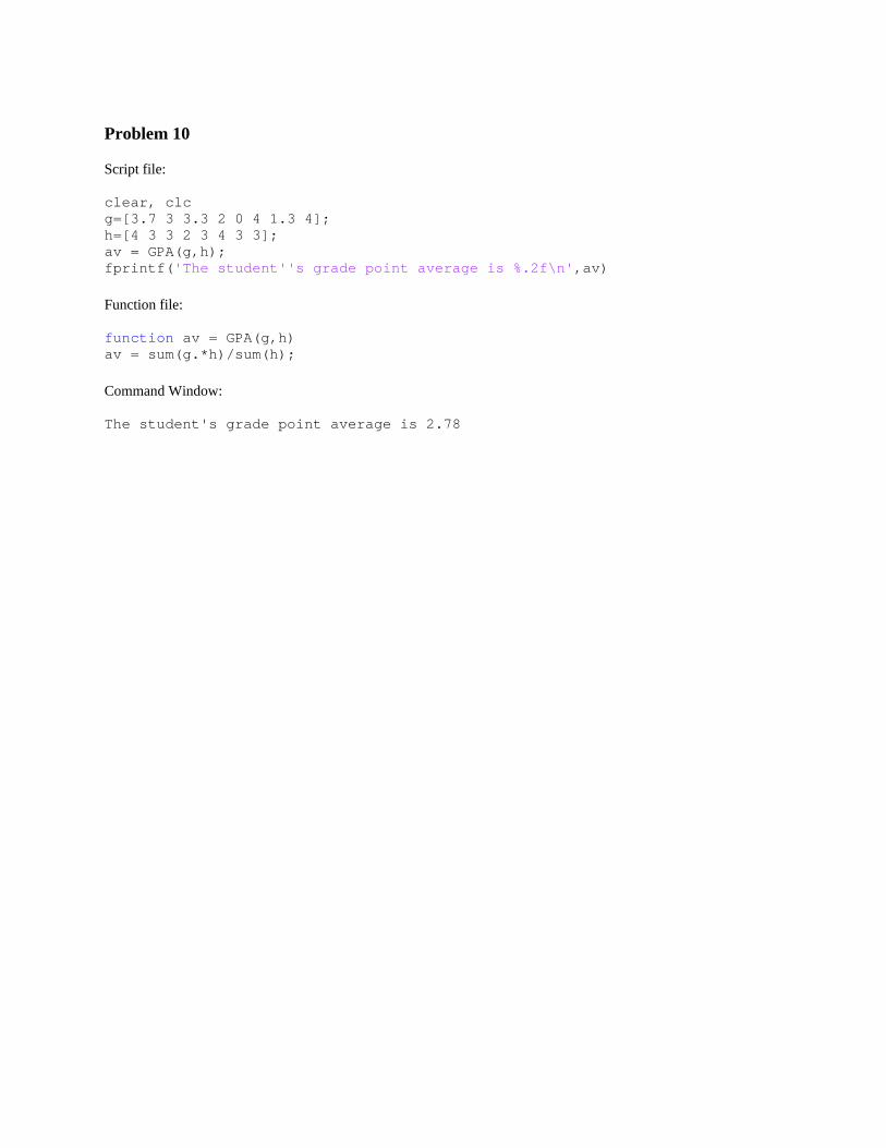
Problem 10
Script file:
clear, clc g=[3.7 3 3.3 2 0 4 1.3 4]; h=[4 3 3 2 3 4 3 3]; av = GPA(g,h); fprintf('The student''s grade point average is %.2f\n',av) Function file:
function av = GPA(g,h) av = sum(g.*h)/sum(h); Command Window:
The student's grade point average is 2.78
Problem 11
Script file:
clear, clc disp('Part (a)') x=9; y = fact(x); if y>0 fprintf('The factorial of %i is %i\n\n',x,y) end disp('Part (b)') x=8.5; y = fact(x); if y>0 fprintf('The factorial of %i is %i\n\n',x,y) end disp('Part (c)') x=0; y = fact(x); if y>0 fprintf('The factorial of %i is %i\n\n',x,y) end disp('Part (d)') x=-5; y = fact(x); if y>0 fprintf('The factorial of %i is %i\n\n',x,y) end
Function file:
function y = fact(x) if x<0 y=0; fprintf('Error: Negative number inputs are not allowed\n\n') elseif floor(x)~=x y=0; fprintf('Error: Non-integer number inputs are not allowed\n\n') elseif x==0 y=1; else y=1; for k=1:x y=y*k; end end
Command Window:
Part (a) The factorial of 9 is 362880 Part (b)
Error: Non-integer number inputs are not allowed Part (c) The factorial of 0 is 1 Part (d) Error: Negative number inputs are not allowed
Problem 12
Script file:
clear, clc disp('Part (a)') A=[-5 -1 6]; B=[2.5 1.5 -3.5]; C=[-2.3 8 1]; th = anglines(A,B,C); fprintf('The angle between the points is %.1f degrees\n\n',th) disp('Part (b)') A=[-5.5 0]; B=[3.5,-6.5]; C=[0,7]; th = anglines(A,B,C); fprintf('The angle between the points is %.1f degrees\n\n',th)
Function file:
function th = anglines(A,B,C) BA = A-B; BC = C-B; th=acosd(dot(BA,BC)/(sqrt(sum(BA.^2))*sqrt(sum(BC.^2))));
Command Window:
Part (a) The angle between the points is 56.9 degrees Part (b) The angle between the points is 39.6 degrees
Problem 13
Script file:
clear, clc disp('Part (a)') A=[1.2 3.5]; B=[12 15]; n=unitvec(A,B); disp('The unit vector is:') disp(n) disp('Part (b)') A=[-6 14.2 3]; B=[6.3 -8 -5.6]; n=unitvec(A,B); disp('The unit vector is:') disp(n) Function file:
function n=unitvec(A,B) n=(B-A)/sqrt(sum((B-A).^2)); Command Window:
Part (a) The unit vector is: 0.6846 0.7289 Part (b) The unit vector is: 0.4590 -0.8284 -0.3209
function w = crosspro(u,v) n=length(u); if n == 2 u(3)=0; v(3)=0; end w(1)=u(2)*v(3)-u(3)*v(2); w(2)=u(3)*v(1)-u(1)*v(3); w(3)=u(1)*v(2)-u(2)*v(1); Command Window:
Part (a) The cross product vector is: 0 0 -175.9000 Part (b) The cross product vector is: -55.5200 -14.7000 -41.4600
Problem 15
Script file:
clear, clc disp('Part (a)') A=[1,2]; B=[10,3]; C=[6,11]; Area = TriArea(A,B,C); fprintf('The area of the triangle is %.1f\n\n',Area) disp('Part (b)') A=[-1.5, -4.2, -3]; B=[-5.1, 6.3, 2]; C=[12.1, 0, -0.5]; Area = TriArea(A,B,C); fprintf('The area of the triangle is %.1f\n\n',Area)
Function files:
function Area = TriArea(A,B,C) [AB AC] = sides(A,B,C); Area = sqrt(sum(crosspro(AB,AC).^2))/2; end function [AB AC] = sides(A,B,C) AB = B-A; AC = C-A; end function w = crosspro(u,v) n=length(u); if n == 2 u(3)=0; v(3)=0; end w(1)=u(2)*v(3)-u(3)*v(2); w(2)=u(3)*v(1)-u(1)*v(3); w(3)=u(1)*v(2)-u(2)*v(1); end Command Window:
Part (a) The area of the triangle is 38.0 Part (b) The area of the triangle is 87.9
Problem 16
Script file:
clear, clc disp('Part (a)') A=[1,2]; B=[10,3]; C=[6,11]; cr = cirtriangle(A,B,C); fprintf('The perimeter of the triangle is %.1f\n\n',cr) disp('Part (b)') A=[-1.5, -4.2, -3]; B=[-5.1, 6.3, 2]; C=[12.1, 0, -0.5]; cr = cirtriangle(A,B,C); fprintf('The perimeter of the triangle is %.1f\n\n',cr)
disp('Part (a)') d=100; b = Bina(d); if b>=0 disp('The binary decomposition is:') disp(b) end disp('Part (b)') d=1002; b = Bina(d); if b>=0 disp('The binary decomposition is:') disp(b) end disp('Part (c)') d=52601; b = Bina(d); if b>=0 disp('The binary decomposition is:') disp(b) end disp('Part (d)') d=2000090; b = Bina(d); if b>=0 disp('The binary decomposition is:') disp(b) end
Function file:
function b = Bina(d) if d>=2^16 b=-1; fprintf('The integer is too large for this routine\n') else n=floor(log(d)/log(2)); b=[]; for k=n:-1:0 p=floor(d/2^k); b=[b p]; d=d-p*2^k; end end Command Window:
Part (a) The binary decomposition is: 1 1 0 0 1 0 0 Part (b) The binary decomposition is: 1 1 1 1 1 0 1 0 1 0 Part (c) The binary decomposition is: Columns 1 through 13 1 1 0 0 1 1 0 1 0 1 1 1 1 Columns 14 through 16 0 0 1 Part (d) The integer is too large for this routine
Problem 19
Script file:
A=[1.5, 3]; B=[9,10.5]; C=[6,-3.8]; TriCirc(A,B,C) Function file:
Part (a) r = 16.8451 th = 35.0215 Part (b) r = 19.7048 th = 112.5663
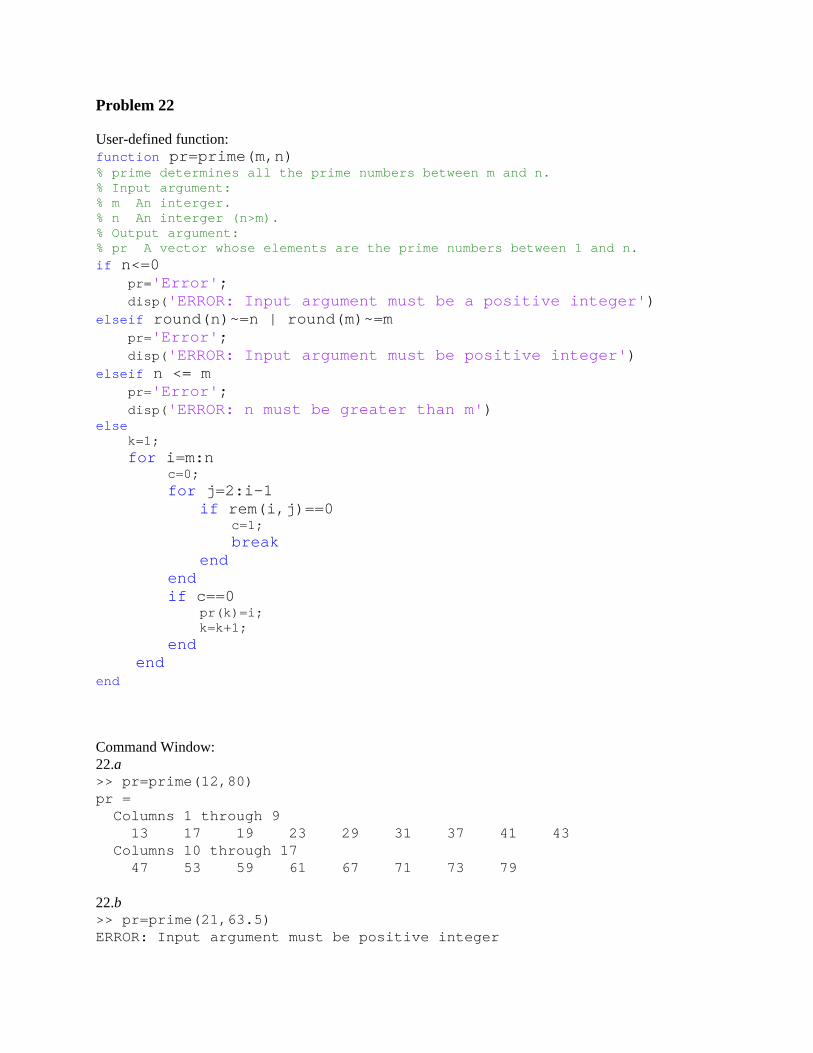
Problem 22
User-defined function: function pr=prime(m,n) % prime determines all the prime numbers between m and n. % Input argument: % m An interger. % n An interger (n>m). % Output argument: % pr A vector whose elements are the prime numbers between 1 and n. if n<=0 pr='Error'; disp('ERROR: Input argument must be a positive integer') elseif round(n)~=n | round(m)~=m pr='Error'; disp('ERROR: Input argument must be positive integer') elseif n <= m pr='Error'; disp('ERROR: n must be greater than m') else k=1; for i=m:n c=0; for j=2:i-1 if rem(i,j)==0 c=1; break end end if c==0 pr(k)=i; k=k+1; end end end
function GM = Geomean(x) GM = prod(x)^(1/length(x)); end
Command Window:
GeometricMeanInflation = 1.0648
Problem 24
User-defined function: function [theta, radius]=CartesianToPolar(x,y) radius= sqrt(x^2+y^2); theta=acos(abs(x)/radius)*180/pi; if (x<0)&(y>0) theta=180-theta; end if (x>0)&(y<0) theta=-theta; end if (x<=0)&(y<0) theta=theta-180; end Command Window: >> [th_a, radius_a]=CartesianToPolar(14,9) th_a = 32.7352 radius_a = 16.6433 >> [th_b, radius_b]=CartesianToPolar(-11,-20) th_b = -118.8108 radius_b = 22.8254 >> [th_c, radius_c]=CartesianToPolar(-15,4) th_c = 165.0686 radius_c = 15.5242 >> [th_d, radius_d]=CartesianToPolar(13.5,-23.5) th_d = -60.1240 radius_d = 27.1017
Problem 25
Function file:
function m=mostfrq(x) n=length(x); a=x==x(1); av=x(a); b(1,1)=av(1); b(1,2)=length(av); j=2; for i=2:n flag=1; for k=1:j-1 if x(i)==b(k,1) flag=0; end end if flag==1 a=x==x(i); av=x(a); b(j,1)=av(1); b(j,2)=length(av); j=j+1; end end [tmax ni]=max(b(:,2)); tmaxi=b==tmax; tmaxtot=sum(tmaxi(:,2)); if tmaxtot > 1 m=('There in more than one value for the mode.'); else m(1,1)=b(ni,1); m(1,2)=tmax; end Command Window:
>> d=randi(10,1,20) d = 1 3 9 1 10 8 5 6 3 5 10 6 6 3 5 7 7 4 4 10 >> m=mostfrq(d) m = There in more than one value for the mode. >> d=randi(10,1,20) d = 1 9 10 8 1 3 4 7 2 8 2 7 5 8 8 10 9 4 7 2 >> m=mostfrq(d) m = 8 4 >> d=randi(10,1,20)
d = 1 8 6 5 10 7 7 9 9 6 2 3 9 1 5 2 10 8 6 5 >> m=mostfrq(d) m = There in more than one value for the mode.
Problem 26
Script file:
x=randi([-30 30],1,14) y=downsort(x) Function file:
function y=downsort(x) y=x; n=length(y); for k=1:n-1 for j=k+1:n if y(k)<y(j) temp=y(k); y(k)=y(j); y(j)=temp; end end end Command Window:
function B = matrixsort(A) [n,m]=size(A); ntm=n*m; C=reshape(A',1,ntm); D=downsort(C); B=reshape(D,m,n)'; function y=downsort(x) y=x; n=length(y); for k=1:n-1 for j=k+1:n if y(k)<y(j) temp=y(k); y(k)=y(j); y(j)=temp; end end end Command Window:
function d3 = det3by3(A) d3=A(1,1)*det2by2(A(2:3,2:3)) - A(1,2)*det2by2(A(2:3,[1 3])) + ... A(1,3)*det2by2(A(2:3,1:2)); function d2 = det2by2(B) d2=B(1,1)*B(2,2)-B(1,2)*B(2,1); Command Window:
Part (a) d3 = -39 Part (b) d3 = -36.3000
Problem 30 Script file:
disp('Part (a)') S=[160, -40, 60]; th=20; disp('Stress in x''-y'' coordinate system in MPa') Stran = StressTrans(S,th) disp('Part (b)') S=[-18, 10, -8]; th=20; disp('Stress in x''-y'' coordinate system in ksi') Stran = StressTrans(S,65) Function file: function Stran = StressTrans(S,th) Stran(1)=0.5*(S(1)+S(2)) + 0.5*(S(1)-S(2))*cosd(2*th) + S(3)*sind(2*th); Stran(2)=S(1)+S(2)-Stran(1); Stran(3)=-0.5*(S(1)-S(2))*sind(2*th) + S(3)*cosd(2*th); end Command Window:
Part (a) Stress in x'-y' coordinate system in MPa Stran = 175.1717 -55.1717 -18.3161 Part (b) Stress in x'-y' coordinate system in ksi Stran = -1.1293 -6.8707 15.8669
function x=lotto(a,b,n) v=rand(1,n); list=a:b; x=[]; for k=1:n index=round(v(k)*(length(list)-1)+1.5); x(k)=list(index); list(index)=[]; end Command Window:
Part (a) x = 45 23 34 6 4 33 48 Part (b) x = 65 52 59 57 51 56 54 63 Part (c) x = -17 -12 -21 -9 -19 -8 -7 -6 -15
Problem 33
Script file:
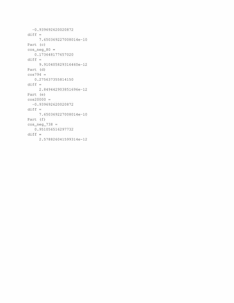
format short g disp('Part (a)') cos67=cosTay(67) diff=abs(cosd(67)-cos67) disp('Part (b)') cos200=cosTay(200) diff=abs(cosd(200)-cos200) disp('Part (c)') cos_neg_80=cosTay(-80) diff=abs(cosd(-80)-cos_neg_80) disp('Part (d)') cos794=cosTay(794) diff=abs(cosd(794)-cos794) disp('Part (e)') cos20000=cosTay(20000) diff=abs(cosd(20000)-cos20000) disp('Part (f)') cos_neg_738=cosTay(-738) diff=abs(cosd(-738)-cos_neg_738) Function file:
function y=cosTay(x) format long if abs(x/360) >= 1 x=x-fix(x/360)*360; end xrad=x*pi/180; sum=0; for i=1:1000 n=i-1; sum=sum+(((-1)^n)*(xrad^(2*n))/factorial(2*n)); S(i)=sum; if i>=2 E=abs((S(i)-S(i-1))/S(i-1)); if E<=0.0000001 break end end end y=sum; Command Window:
Part (a) cos67 = 0.390731128591239 diff = 1.019652695610773e-10 Part (b) cos200 =
-0.939692620020872 diff = 7.650369227008014e-10 Part (c) cos_neg_80 = 0.173648177657020 diff = 9.910405829316460e-12 Part (d) cos794 = 0.275637355814150 diff = 2.849442903851696e-12 Part (e) cos20000 = -0.939692620020872 diff = 7.650369227008014e-10 Part (f) cos_neg_738 = 0.951056516297732 diff = 2.578826041599314e-12
Problem 34
Script file:
w=10; h=7; d=1.75; t=0.5; yc=centroidU(w,h,t,d) Function file:
function yc = centroidU(w,h,t,d) yc=(d*(w-2*t)*(h-d/2)+t*h^2)/(2*h*t+d*(w-2*t)); Command Window:
yc =
5.3173
Problem 35
Script file:
w=12; h=8; d=2; t=0.75; Ixc=IxcTBeam(w,h,t,d) Function files:
function Ixc = IxcTBeam(w,h,t,d) yc = centroidU(w,h,t,d); Ixc = 2*(t*h^3/12+t*h*(h/2-yc)^2) + (w-2*t)*d^3+(w-2*t)*d*(h-d/2-yc)^2; function yc = centroidU(w,h,t,d) yc=(d*(w-2*t)*(h-d/2)+t*h^2)/(2*h*t+d*(w-2*t)); Command Window:
Ixc =
216.7273
Problem 36
Script file:
R=input('Please input the size of the resistor: '); L=input('Please input the size of the inductor: '); %can use logspace or explicitly create an appropriate array for w power=1:.01:6; w=10.^power; RV=LRFilt(R,L,w); semilogx(w,RV) title('LR Circuit Response') xlabel('Frequency, rad/s') ylabel('Throughput') Function file:
function RV=LRFilt(R,L,w) RV=1./sqrt(1+(w*L/R).^2); Command Window:
Please input the size of the resistor: 600
Please input the size of the inductor: 0.14e-6
Figure Window:
101 102 103 104 105 1061
1
1
1
1
1
1LR Circuit Response
Frequency, rad/s
Thro
ughp
ut
Problem 37
Script file:
C=160*10^-6; L=.045; R=200; %note can use logspace or explicitly create appropriate array of w power=1:.01:4; w=10.^power; RV1=filtfreq(R,C,L,w); R=50; RV2=filtfreq(R,C,L,w); semilogx(w,RV1,w,RV2,'--') title('Circuit Response') xlabel('Frequency, rad/s') ylabel('Throughput') legend('R=200','R=50') Function file:
function RV = filtfreq(R,C,L,w) RV= abs(R*(1-w.^2*L*C))./sqrt((R-R*w.^2*L*C).^2 + (w*L).^2); Figure Window:
art (a)') new] = ro') art (b)') 9; .^2+1.5; new]=rotay,xnew,ynrotation 'y=(x-7)^'x-->') 'y-->') 10 0 10])
file:
n [xr,yr] sd(q) -y*nd(q) + y
Window:
)
035
503
ndow:
tation(6.5,
tion(x,y,25ew,':') test') 2+1.5','25
= rotationsind(q); *cosd(q);
,2.1,25)
5);
degree ro
n(x,y,q)
otation')
Problem 40
Script file:
disp('Part (a)') prob3of6 = ProbLottery(3,6,49) disp(' ') disp('Part (b)') num=0:6; odds=ProbLottery(num,6,49); tbl=[num;odds]; disp(' ') disp(' Number') disp(' Correct Odds') fprintf(' %1i %.9f\n',tbl) fprintf('\nCheck: The sum of the probabilities is %.9f\n',sum(odd Function files:
function P = ProbLottery(m,r,n) P=Cxy(r,m).*Cxy(n-r,r-m)./Cxy(n,r); function C = Cxy(x,y) C=factorial(x)./(factorial(y).*factorial(x-y)); Command Window:
Part (a) prob3of6 = 0.0177 Part (b) Number Correct Odds 0 0.435964976 1 0.413019450 2 0.132378029 3 0.017650404 4 0.000968620 5 0.000018450 6 0.000000072 Check: The sum of the probabilities is 1.000000000
1
Chapter 8 Solved Problems
Problem 1Script file:
clear, clc
p=[0.1 -0.2 -1 5 -41.5 235];
x=linspace(-6,6,200);
y=polyval(p,x);
plot(x,y)
xlabel('x')ylabel('y')
Figure:
-6 -4 -2 0 2 4 6-200
-100
0
100
200
300
400
500
x
y
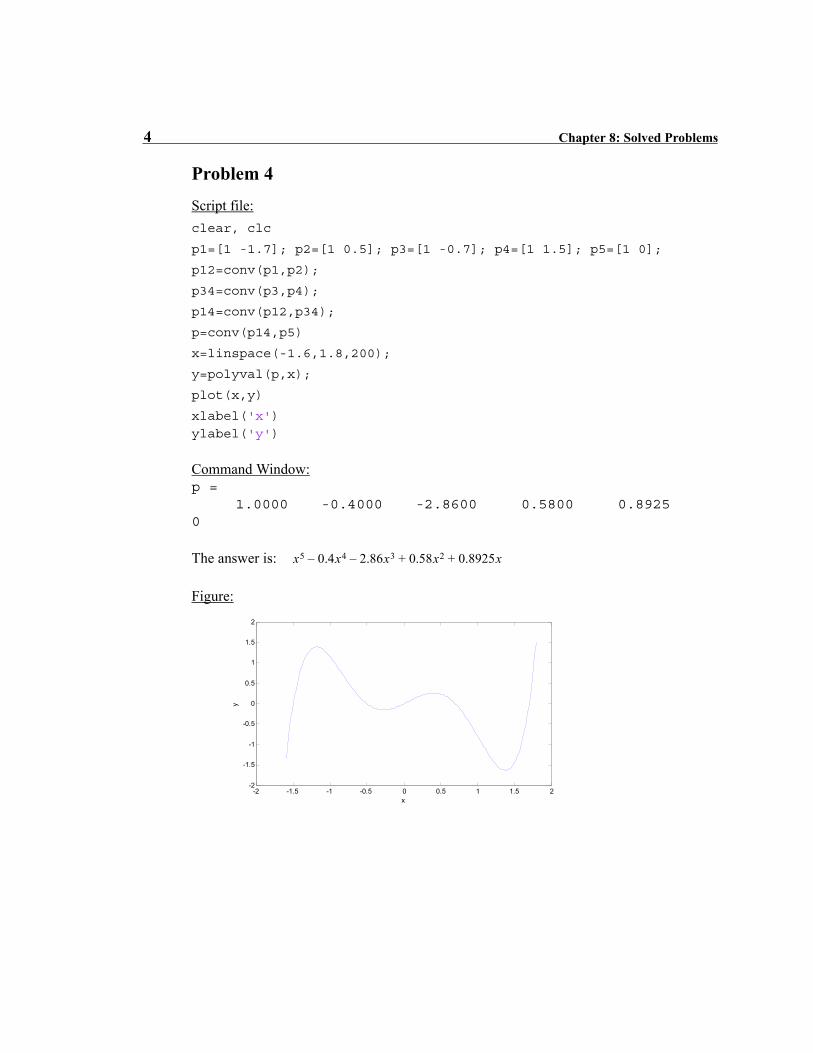
2 Chapter 8: Solved Problems
Problem 2Script file:
clear, clc
p=[0.008 0 -1.8 -5.4 54];
x=linspace(-14,16,200);
y=polyval(p,x);
plot(x,y)
xlabel('x')ylabel('y')
Figure:
-15 -10 -5 0 5 10 15 20-150
-100
-50
0
50
100
x
y
Chapter 8: Solved Problems 3
Problem 3Script File:
clear, clc
pa=[-1 0 5 -1];
pb=[1 2 0 -16 5];c=conv(pa,pb)
Command Window:
c = -1 -2 5 25 -7 -80 41 -5
The answer is: x7– 2x6– 5x5 25x4 7x3– 80x2– 41x 5–+ + +
When the script file is executed four Figure Windows with the following figuresopen.
0 0.5 1 1.5 2 2.5 3 3.5
x 10
0
0.2
0.4
0.6
0.8
1
1.2
1.4
Height (m)
De
nsi
ty (
kg/m
3)
34 Chapter 8: Solved Problems
(b)Fit the data with exponential function since the data points in the third plot appearto approximately be along a straight line.
Script file: (Determines the constants of the exponential function that best fits thedata, and then plots the function and the points in a linear axes plot.)
Command Window:eqn1 =(T+a)*(v+b)=(T0+a)*beqn2 =a*(v+b) = (T0+a)*bAnswer to part a:vmax =b*T0/aeqn3 =(T+a)*(v+(vmax*a/T0))=(T0+a)*(vmax*a/T0)Answer to part b:v =-vmax*a*(T-T0)/T0/(T+a)
Command Window:Answer to Part a:vs =g/c*m-exp(-c/m*t)*g/c*mAnswer to Part b:cs = 16.1489 0Velocity as a function of time:vst =621285642344595456/11363786546778455-621285642344595456/11363786546778455*exp(-2272757309355691/12666373951979520*t)
Command Window:Part a:Displacement x as a function of time:xs =27/55550*1111^(1/2)*exp(-3/20*t)*sin(1/20*1111^(1/2)*t)+9/50*exp(-3/20*t)*cos(1/20*1111^(1/2)*t)Velocity v as a function of time:v =-252/27775*1111^(1/2)*exp(-3/20*t)*sin(1/20*1111^(1/2)*t)
Part b:Displacement x as a function of time:xs =(9/100+3/460*345^(1/2))*exp(1/10*(-25+345^(1/2))*t)+(-3/460*345^(1/2)+9/100)*exp(-1/10*(25+345^(1/2))*t)Velocity v as a function of time:v =-21/2875*345^(1/2)*(exp(1/10*(-25+345^(1/2))*t)-exp(-1/10*(25+345^(1/2))*t))