Matrix Corrections and Error Analysis in High-Precision SIMS18O/16O Measurements of Ca–Mg–Fe Garnet
Ryan B. Ickert (1,2)* and Richard A. Stern (1)
(1) Canadian Centre for Isotopic Microanalysis, Department of Earth and Atmospheric Sciences, University of Alberta, Edmonton, Canada(2) Current Address: Berkeley Geochronology Center, 2455 Ridge Road, Berkeley, 94709, CA, USA* Corresponding author. e-mail: [email protected]
We report technical and data treatment methods formaking accurate, high-precision measurements of18O/16O in Ca–Mg–Fe garnet utilising the Cameca IMS1280 multi-collector ion microprobe. Matrix effects weresimilar to those shown by previous work, whereby Caabundance is correlated with instrumental mass fraction-ation (IMF). After correction for this effect, there appearedto be no significant secondary effect associated with Mg/Fe2+ for routine operational conditions. In contrast,investigation of the IMF associated with Mn- or Cr-richgarnet showed that these substitutions are significant andrequire a more complex calibration scheme. The Ca-related calibration applied to low-Cr, low-Mn garnet wasreproducible across different sample mounts and under arange of instrument settings and therefore should beapplicable to similar instruments of this type. Therepeatability of the measurements was often better than± 0.2‰ (2s), a precision that is similar to the repeatabilityof bulk techniques. At this precision, the uncertainties dueto spot-to-spot repeatability were at the same magnitudeas those associated with matrix corrections (± 0.1–0.3‰)and the uncertainties in reference materials (± 0.1–0.2‰).Therefore, it is necessary to accurately estimate andpropagate uncertainties associated with these parameters– in some cases, uncertainties in reference materials ormatrix corrections dominate the uncertainty budget.
Nous pr�esentons les m�ethodes techniques et de traitementde donn�ees pour faire des mesures exactes de hautepr�ecision de 18O/16O dans les Ca-Mg-Fe grenats enutilisant la microsonde ionique �a multicollection CamecaIMS 1280. Les effets de matrice sont similaires �a ceuxpr�esent�es par les travaux pr�ec�edents, dans lesquellesl’abondance en Ca a �et�e corr�el�ee avec le fractionnementdemasse instrumental (IMF). Apr�es correction de cet effet, ilsemble n’y avoir aucun effet secondaire associ�e �aMg/Fe2+ dans des conditions op�erationnelles de routine.En revanche, l’�etude du IMF associ�e avec les grenats richesen Mn ou en Cr a montr�e que ces substitutions sontimportantes et n�ecessitent un syst�eme de calibration pluscomplexe. L’�etalonnage bas�e sur le Ca appliqu�e �a desgrenats pauvres en Cr ou Mn est reproductible pour lesdiff�erents montages d’�echantillons et dans une gamme der�eglages de l’instrument, et devrait donc etre applicable �ades appareils similaires. La r�ep�etabilit�e des mesures estsouvent meilleure que ± 0.2‰ (2s), une pr�ecision qui estsemblable �a la r�ep�etabilit�e des techniques en vrac (‘bulk’).Pour cette pr�ecision, les incertitudes li�ees �a la r�ep�etabilit�epoint �a point sont du meme ordre de grandeur que cellesassoci�es �a des corrections matricielles (± 0.1–0.3‰) et lesincertitudes des mat�eriaux de r�ef�erence (± 0.1–0.2‰). Parcons�equent, il est n�ecessaire d’�evaluer avec pr�ecision et depropager les incertitudes associ�ees �a ces param�etres -dans certains cas, les incertitudes sur les mat�eriaux der�ef�erence ou les corrections matrice dominer le budgetd’incertitude.
Mots-clés : SIMS, effet de matrice, isotopes stables, estimationde l’incertitude, �el�ements de faible num�ero atomique.Received 08 Nov 12 – Accepted 11 Mar 13
For oxygen isotope determination of oxygen-rich min-erals by secondary ion mass spectrometry (SIMS), the areasof application and the corresponding precision andaccuracy required typically fall into two broad areas. For
cosmochemical applications, isotope ratio variations areoften large, and the corresponding precision and accuracyneeded can be comparatively modest (e.g., > � 1‰ for18O/16O). For terrestrial applications, particularly those
involving high-temperature minerals, the isotopic variationsmay be considerably smaller, and a much higher level ofprecision and accuracy is often required.
For SIMS 18O/16O analysis of silicate minerals with thelatest instrumentation and techniques, the repeatability ofindividual spot analyses (consuming ng–pg of material) onnominally homogeneous reference materials (RMs) during asingle analytical session can be better than 0.2‰ (2s, e.g.,Kita et al. 2009) This level of precision and accuracy hasbeen made possible through a combination of progressivetechnical and procedural innovations and improvements tocalibration in chemically complex minerals. At its best, thespot-to-spot repeatability of SIMS analysis approaches thatof bulk (mg) analyses of silicate minerals by fluorination anddual-inlet isotope ratio mass spectrometry (Clayton andMayeda 1963, Valley et al. 1995), which is the de factostandard method for determining 18O/16O in these mate-rials.
The useful secondary ion yield of isotopes of the sameelement is highly dependent on the chemistry and structureof the analysed sample (Slodzian 1975, Slodzian et al.1980, Eiler et al. 1997). Termed the matrix effect, itrepresents a major limitation on the accuracy of SIMSisotope determination. A theoretical treatment of matrixeffects precise enough for either cosmochemical or terrestrialapplications is lacking, and therefore, the most accurateSIMS analyses require RMs with matrices exactly matched tothe analysed material. Many minerals of interest have awide range in chemistry, and it is difficult and impractical tohave a RM for each composition. To overcome this problem,various ad hoc correction schemes are employed by mostlaboratories (Jamtveit and Hervig 1994, Eiler et al. 1997,Page et al. 2010).
Garnet is a common target for terrestrial stable isotopestudies. It has the general formula X3Y2Si3O12, where, for thegarnets of interest here, X is mainly occupied by Mg2+, Ca2+,Fe2+ or Mn2+, and Y is occupied by Al3+ or Cr3+ (Deer et al.1982, Locock 2008). It is a relatively common silicate mineral,present in a range of rock types, and is resistant to alteration.The garnet structure is relatively flexible and accommodates awide range of cations and therefore has a wide range inchemical composition (Figure 1), allowing garnet to recordgeological events such as fluid flow, melting, heating andburial. On the other hand, this chemical complexity makes itdifficult to calibrate garnet O-isotope determinations by SIMS.It has been a frequent target for SIMS matrix calibrations(Jamtveit and Hervig 1994, Eiler et al. 1997, Vielzeuf et al.2005, Page et al. 2010), which have progressed in parallelwith improved SIMS techniques.
In this study, we advance the SIMS method of garnetO-isotope determination by firstly, refining the scheme tocorrect the main matrix effect due to Ca substitution (Vielzeufet al. 2005, Page et al. 2010); secondly, addressing the roleof variable Mg/Fe, Cr and Mn; and thirdly, presenting a fullaccounting of the uncertainty budget.
Experimental set-up
All measurements were undertaken on the CanadianCentre for Isotopic Microanalysis Cameca IMS 1280 instru-ment (CAMECA, Gennevilliers, France). The IMS 1280 is aforward-geometry double-focussing large-format SIMS instru-ment (de Chambost et al. 1998), fitted with an obliqueincidenceCs+ primary ion source, a normal incidence electrongun (Slodzian et al. 1986, Migeon et al. 1990) and a multi-collector (Migeon et al. 1990, Schuhmacher et al. 2004).
Fragments of several garnet RMs were embedded in two,25 mm-diameter epoxy (West System) mounts, M0025Cand M0095. The fragments were all placed within 5 mm ofthe centre of the mount, where experiments have shown that,for our instrument, there is negligible effect of sample locationon measured isotope ratio (cf. Ickert et al. 2008, Whitehouseand Nemchin 2009). The analytical face of each mount waspolished using wet diamond grit to 0.25 lm, so thattopographic differences between individual fragments andthe epoxy were absent. The polished mount was cleanedusing rinses of de-ionised water, a dilute alkaline cleaningsolution, ethanol, and finally dried in an oven at 40 °C for30 min. The surface was then coated with 25 nm of Au usingan evaporative coater and placed in a standard stainless
Figure 1. Ternary diagram illustrating the variation in
fractional molar quantities of Ca, Fe and Mg, the three
most important chemical components for most of the
garnets analysed. Samples that have other important
cations have different symbols: small amounts of Cr are
denoted by light grey shading, substantial Fe3+ by a
steel Cameca mount holder. The grains on the mount werefirst characterised with a scanning electron microscope, andthen the mount was placed in the sample lock of the IMS1280 at high vacuum for more than 24 hr prior to analysis.
We introduce five new garnet RMs. These have all beencharacterised for d18O in the University of Oregon laserfluorination stable isotope laboratory. Our primary SIMS RM iscalled ‘UAG’ (sample number S0068), a megacrystic pyropegarnet from the Gore Mountain Mine (Bartholom�e 1960).Hundreds of ion microprobe analyses in our laboratory ondozens of randomly selected grains strongly suggest that thissample is homogeneous at better than0.1‰ in 18O/16O. Thegarnet has a composition approximately corresponding to(Mg1.23Fe1.35Ca0.42)Al2Si3O12, with approximately 0.4%m/m MnO and < 0.1% m/m Cr2O3. Seven laser fluorinationanalyses (normalised to a d18Ovsmow of UWG-2 = 5.8‰,Valley et al. 1995) yield a d18Ovsmow of 5.72 � 0.13‰ (alluncertainties are at 95% confidence or 2s unless clearly statedotherwise). We directly compared grains of UWG-2 andUAGin our laboratory by SIMS, yielding a difference in d18O of-0.04 � 0.07‰ between the mean values (UAG–UWG-2;nUAG = 15, nUWG-2 = 15), which is within uncertainty of theapproximately -0.08‰ that is implied by the laser fluorinationtechnique. The similarity between UAG and UWG-2 isexpected since they are derived from the same locality,although we do not suggest that they are indistinguishable orinterchangeable. Sample S0088B is a Ca-rich (see Figure 1)garnet from Jeffrey Mine, Quebec (Akizuki 1989); sampleS0141 is a near end-memberMg–Al garnet fromDoraMaira(Chopin 1984, Sharp et al. 1993); sample S0142 is a Fe-richgarnet from Baffin Island; S0113 is a Cr-rich garnet suppliedby D.G. Pearson (sample AHM35 of Klein-BenDavid andPearson 2009). A large number of chips of S0088B havebeen tested by SIMS for homogeneity; however, to date, theother samples have not been as extensively tested.
Other reference materials used here were provided byJohn Craven (Edinburgh Ion Microprobe Facility) and havebeen previously characterised by other workers. This includessamples described by Eiler et al. (1997; AlmCMG, AlmSE,SpessSE and GrsSE) and by Page et al. (2010; 13-63-20,13-63-21, 13-63-44, 13-63-19, 13-62-27, 13-62-29). Inaddition, garnet AND and LBM11 were characterised byJohn Craven (pers. comm.), where AND is Fe3+-rich andLBM11 is a Cr-rich garnet (Smith and Boyd 1992).
The individual d18O laser fluorination measurements ofthe new reference materials are tabulated in the OnlineSupporting Information. For the internal laboratory databaseof the CCIM, all analysed materials have sequentiallyallocated S-numbers, including those with previously
allocated (alias) sample names. These S-numbers are usedin the naming of individual spot analyses, and therefore, areference guide to the original sample names and CCIM IDnumbers is included in the tables.
For all work, primary beam intensities were between 2.8and 4.1 nA generated from a ~12 lm-diameter Gaussian-focussed 20 keV Cs+ primary beam (impact energy 20 keVdue to -10 kV sample potential) that was rastered (using thedynamic transfer optical system, DTOS, to maintain second-ary beam alignment) at 8 lm 9 8 lm continuously duringanalysis to minimise fractionation effects from the change inpit geometry during sputtering. Negative secondary ionswere extracted and accelerated through a total of 10 kV. Anormal incidence electron gun was utilised to avoid positivecharging at the sputter site.
A single-spot measurement consisted of a raster period of30 s on the sample surface that was slightly larger than thespot size to sputter the Au coat, implant Cs and reach anapproximate steady state. Following the raster, the secondarybeam was automatically centred in the field aperture (FA;5 mm 9 5 mm) and entrance slit (122 lm). Data for 18Oand 16O were collected simultaneously on Faraday cups inthe multi-collector array (L′2 and H1 positions) using 1010
and 1011 Ω resistors, respectively, and the largest exit slits(500 lm) were utilised. Mass resolution (10% definition)for 18O- was ~ 2300. Secondary ion intensities were3.5–5.5 GHz for 16O with a 50 eV energy window, and2–3 GHz with a 20 eV window. Data were collected incycles of 5 s, with either 15 (M0095) or 20 (M0025C) cycles.Amplifier baselines were measured for 30 s at the beginningof each analytical session and subtracted from each mea-surement. Amplifier gains were determined electronically.
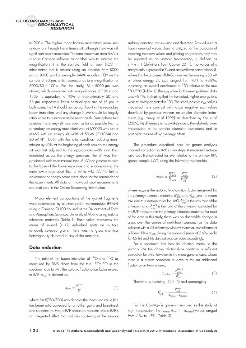
The two mounts in question (M0025C and M0095)were analysed over four analytical sessions (IP11061, 62,84, 86), each with slightly different instrument tunings. A‘session’ (denoted as IP11xxx) refers to a period of time(typically several hours) in which the instrumental massfractionation (IMF) was either constant or changing system-atically, and the data from that period were processedtogether. Mount M0025C was run with two different transfermagnification settings in order to evaluate the effect ofvariations in transmission into the mass analyser. In onesession (IP11061), the transfer magnification was set at1009 (‘MA80’), and then in an immediately followingsession (IP11062), it was set at 1339 (‘MA60’), the latterhaving ~ 15% higher transmission through the entrance slit.The transfer magnification is a parameter defined by the ratioof the sampled surface dimension to that in the FA. Typicalmagnifications for isotopic determination ranged from 1009
to 2009. The higher magnification transmitted more sec-ondary ions through the entrance slit, although there was stillsignificant beam truncation. The term ‘maximum area’ (MA) isused in Cameca software as another way to indicate themagnification: it is the sample field of view (FOV) inmicrometres that is present using an arbitrary FA = 8000lm 9 8000 lm. For example, MA80 equals a FOV on thesample of 80 lm, which corresponds to a magnification of8000/80 = 1009. For this study, FA = 5000 lm wasutilised, which combined with magnifications of 1009 and1339 is equivalent to FOVs of approximately 50 and38 lm, respectively. For a nominal spot size of 15 lm, inboth cases, the FA should not be significant in the secondarybeam truncation, and any change in IMF should be largelyattributable to truncation at the entrance slit. During those twosessions, the energy slit was open as far as possible (i.e., nosecondary ion energy truncation). Mount M0095 was run atMA60 with an energy slit width of 50 eV (IP11084) and20 eV (IP11086), with the latter condition reducing trans-mission by 40%. At the beginning of each session, the energyslit was first adjusted to the appropriate width, and thentranslated across the energy spectrum. The slit was thenpositioned such as to transmit ions -5 eV and greater relativeto the base of the low-energy ions and encompassing themain low-energy peak (i.e., -5 eV to +45 eV). No furtheradjustment or energy scans were done for the remainder ofthe experiments. All data on individual spot measurementsare available in the Online Supporting Information.
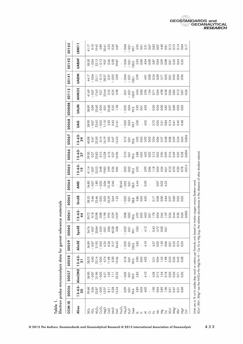
Major element compositions of the garnet fragmentswere determined by electron probe microanalysis (EPMA),using a Cameca SX100 housed at the Department of Earthand Atmospheric Sciences, University of Alberta using naturalreference materials (Table 1). Each value represents themean of several (> 12) individual spots on multiplerandomly selected grains. There was no gross chemicalheterogeneity detected in any of the materials.
Data reduction
The ratio of ion beam intensities of 18O and 16O asmeasured by SIMS differs from the true 18O/16O in thespecimen due to IMF. The isotopic fractionation factor relatedto IMF, aIMF, is defined as
aIMF � Rraw
Rtð1Þ
where R is R(18O/16O), raw denotes the measured value (theion beam ratio corrected for amplifier gains and baselines),and tdenotes the true, or IMF-corrected, reference value. IMF isan integrated effect that includes sputtering at the sample
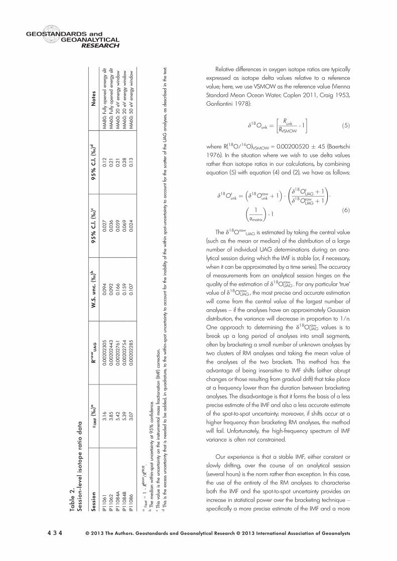
surface, ionisation, transmission and detection. Raw values ofahave numerical values close to unity, so for the purposes ofreporting their raw values and plotting on graphics, they maybe reported as an isotopic fractionation, e, defined ase ≡ a - 1 (definitions from Coplen 2011). The values of eare typically expressed in‰andare similar to conventional d-values. For the analyses of UAGpresented here using a50 eVor wider energy slit, eIMF ranged from +3.1 to +3.8‰,indicating an overall enrichment in 18O relative to the true18O/16O (Table 2). The eIMF value for the energy-filtered datawas +5.4‰, indicating that the truncated, higher-energy ionswere relatively depleted in 18O. The small, positive eIMF valuesmeasured here contrast with large, negative eIMF valuesdescribed by previous workers on smaller diameter instru-ments (e.g., Hervig et al. 1992). As described by Kita et al.(2009), this difference is mostly likely due to the relatively lowertransmission of the smaller diameter instruments and inparticular the use of high-energy offsets.
The procedure described here for garnet analysesinvolved correction for IMF in two steps. A measured isotoperatio was first corrected for IMF relative to the primary RM,garnet sample UAG, using the following relationship.
aUAG � RrawUAG
RtUAG¼ Rrawunk
RUAGunk
ð2Þ
where aUAG is the isotopic fractionation factor measured forthe primary reference material, RrawUAG and RtUAGare the meanraw and true isotope ratios for UAG, Rrawunk is the raw ratio of theunknown and RUAGunk is the ratio of the unknown corrected forthe IMF measured in the primary reference material. For mostof the data in this study, there was no discernible change inaUAG over the course of multi-hour sessions. For the datacollectedwith a20 eV energywindow, therewasa small amountof linear drift in aUAG during the analytical session (0.16‰ per hrfor 4.5 hr), and this data set was corrected accordingly.
For a specimen that has an identical matrix to theprimary RM, the above relationships constitute a sufficientcorrection for IMF. However, in the more general case, wherethere is a matrix correction to account for, an additionalfractionation term is used,
amatrix ¼RUAGunk
Rtunkð3Þ
Therefore, substituting (2) in (3) and rearranging,
Rtunk ¼Rrawunk
aUAG � amatrixð4Þ
For the Ca–Mg–Fe garnets measured in this study athigh transmission, the ematrix (i.e., 1 - amatrix) values rangedfrom -1‰ to +3‰ (Table 3).
Relative differences in oxygen isotope ratios are typicallyexpressed as isotope delta values relative to a referencevalue; here, we use VSMOW as the reference value (ViennaStandard Mean Ocean Water; Coplen 2011, Craig 1953,Gonfiantini 1978):
d18Ounk ¼Runk
RVSMOW- 1
� �ð5Þ
where R(18O/16O)VSMOW = 0.00200520 � 45 (Baertschi1976). In the situation where we wish to use delta valuesrather than isotope ratios in our calculations, by combiningequation (5) with equation (4) and (2), we have as follows:
d18Otunk ¼ d18Oraw
unk þ 1� �
� d18OtUAG þ 1
d18OrawUAG þ 1
!�
1amatrix
� �- 1
ð6Þ
The d18OrawUAG is estimated by taking the central value
(such as the mean or median) of the distribution of a largenumber of individual UAG determinations during an ana-lytical session during which the IMF is stable (or, if necessary,when it can be approximated by a time series). The accuracyof measurements from an analytical session hinges on thequality of the estimation of d18Oraw
UAG . For any particular ‘true’value of d18Oraw
UAG , the most precise and accurate estimationwill come from the central value of the largest number ofanalyses – if the analyses have an approximately Gaussiandistribution, the variance will decrease in proportion to 1/n.One approach to determining the d18Oraw
UAG values is tobreak up a long period of analyses into small segments,often by bracketing a small number of unknown analyses bytwo clusters of RM analyses and taking the mean value ofthe analyses of the two brackets. This method has theadvantage of being insensitive to IMF shifts (either abruptchanges or those resulting from gradual drift) that take placeat a frequency lower than the duration between bracketinganalyses. The disadvantage is that it forms the basis of a lessprecise estimate of the IMF and also a less accurate estimateof the spot-to-spot uncertainty; moreover, if shifts occur at ahigher frequency than bracketing RM analyses, the methodwill fail. Unfortunately, the high-frequency spectrum of IMFvariance is often not constrained.
Our experience is that a stable IMF, either constant orslowly drifting, over the course of an analytical session(several hours) is the norm rather than exception. In this case,the use of the entirety of the RM analyses to characteriseboth the IMF and the spot-to-spot uncertainty provides anincrease in statistical power over the bracketing technique –
specifically a more precise estimate of the IMF and a moreTable
accurate estimate of repeatability uncertainty. This method isthe standard one utilised in tracking IMF during SIMS U–Pbanalysis sessions. In situations where IMF was unsystemati-cally varying over periods less than an hour, the bracketingmethod would be required. The point here is to emphasisethat there is no one ‘best practice’ method for correcting forIMF, as it will depend on the analytical performance actuallyobserved most commonly in a specific laboratory.
Values ofaUAG candiffer by several‰between analyticalsessions, betweenmounts or with the specific tuning conditionsof the instrument (cf. Table 2). In contrast, for a limited but usefulrange of IMS 1280 instrumental parameters, the values ofamatrix, that is, the ratio of the UAG-normalised isotope ratiosand the true isotope ratios, have a regular and highlyreproducible relationship with garnet composition (as docu-mented below, and in Table 3). This knowledge allows theinitial and ongoing use of a RM mount containing a largenumber of reference materials to determine and verify amatrix
as a function of garnet composition (cf. Page et al. 2010). Thisamatrix vs. garnet composition relationship can then beappliedto analyses of unknowns on a separatemount, employing onlyUAG to determine aUAG and a secondary RM (preferably onewith a large amatrix such as S0088B) to serve as a check on theassumed value of amatrix.
Results and discussion
Matrix effects
Instrumental mass fractionation is an integrated effectthat combines the sputtering process, transmission into andthrough the mass spectrometer and the vagaries of thedetection system. Although it is known that sputtering caninduce isotopic fractionation (Russell et al. 1980), the massspectrometer itself imposes an important component (Eileret al. 1997, Vielzeuf et al. 2005). IMF is also a function ofthe composition and structure of the material analysed(Slodzian 1980, Hervig et al. 1992, Eiler et al. 1997,Riciputi et al. 1998, Vielzeuf et al. 2005, Page et al. 2010).Early work on small-diameter ion microprobes found arelationship between IMF and formula weight (Hervig et al.1992), as well as sputter rate, the latter implying thatvariations in energy transfer efficiency were important ininducing matrix effects (Eiler et al. 1997). Later work withlarge-geometry instruments found that these relationshipsdid not hold when accepting a wider energy range of ions(Vielzeuf et al. 2005, Page et al. 2010) illustrating theimportant role of instrumentation in matrix effects.
Vielzeuf et al. (2005) demonstrated that for Fe–Mg–Cagarnets, the matrix effect was a regular function of garnet
chemistry. They modelled the relationship between IMF andchemical composition as a linear function of four chemicalend members (Ca–Fe–Mg–Mn). Their correction assumedthat matrix effects were linear and that they combine linearly– that is, that a Ca effect and a Mn effect is equal to the sumof the two effects on their own. Their data reduction schemewas accurate to within ~ 0.6‰.
Page et al. (2010), building on the work of Vielzeuf et al.(2005), modelled the matrix-related IMF as a quadraticfunction of the sum of the grossular (CaAl) and uvarovite(CaCr) components of so-called pyralspite (pyrope–alman-dine–spessartine, or Mg–Fe2+–Mn) garnets. They alsointroduced a similar model relating IMF to the sum of theandradite (CaFe3+) and a schorlomite-like (CaTi) garnet forso-called ugrandite (uvarovite–grossular–andradite, Ca–Cr–Fe3+) garnets; however, these latter series of garnets are notconsidered here. Their non-linear correction ignored Mg–Fevariations, but increased the accuracy of d18O values of RMby about a factor of two.
Calibration: The calibration for matrix effects here usesa similar scheme to Page et al. (2010). For this calibration,we only used those RMs that are dominated by Ca–Mg–Fein the octahedral site and Al in the dodecahedral site. Byassuming that the minor components induce a negligibleadditional matrix effect, this reduces number of uniquechemical vectors to two. In contrast to previous work (Vielzeufet al. 2005, Page et al. 2010), we used the molar ratio ofCa/(Mg+Fe2++Ca) (abbreviated as XCa*, as it excludesother dodecahedral cations like Mn), which, for thesegarnets, is effectively the occupancy of Ca on the dodeca-hedral site.
Page et al. (2010), instead, cast their matrix correction interms of the sum of the relative abundances of mineral endmembers. Expressing garnet in terms of the proportions ofmineral end members is a common procedure in mineral-ogy – it can clarify the relationships between the chemicalabundances in complex minerals. However, these calcula-tions are non-unique and depend on how cations areallocated to mineral end members. For example, Page et al.(2010) elected to use the CaCr end member rather than theMgCr (knorringite) end member, which, for many naturalgarnets, is a suitable decision as Ca and Cr are stronglycorrelated in many suites of garnets, although for otherimportant suites (in particular, Mg- and Cr-rich mantle-derived garnets), it is not. More importantly, it makes theimplicit assumption that the magnitude and direction of thematrix-related mass bias associated with Cr is identical toCa. The Cr abundances in the garnets studied by Page et al.were not high enough for this to make a difference to their
work; however, the behaviour of Cr is implicit in their model,but was not explicitly tested.
The measured 18O/16O on RMs from session IP11086(Table 3) has been used to determine the relationshipbetween amatrix and XCa*. Following Page et al. (2010), weused the functional form aMatrix ¼ A � X2
Ca� þ B � XCa� þ C .The data and the derived calibration curve are plotted inFigure 2 as ematrix vs. XCa*, which shows the effect ofcomposition on mass bias. The ematrix values are plotted(rather than amatrix) for clarity, as they have simpler numericalvalues. For each RM in the calibration, the apparent amatrix
and 95% confidence limits were determined by taking themean and the 95% confidence limits of the mean (thestandard error multiplied by the Student’s t multiplier for ap-value of 0.05 and n - 1 degrees of freedom) for each spotanalysed in that session. The A, B andC parameters were thenrecovered by minimising the chi-square function and wereA = -0.00457 � 0.00152, B = 0.008635 � 0.00158and C = 0.99889 � 0.00018 with Pearson’s correlationcoefficients of qA,B = -0.982; qA,C = -0.72; andqB,C = -0.78. The calibration curve is remarkably close tothat published by Page et al. (2010), differing by < 0.1‰.
Repeatability of matrix effects: It is not efficient toplace all available RMs on each epoxy mount for eachanalysis. For this calibration scheme to be useful, it must berobust to small changes in instrument tuning and berepeatable from mount to mount. The method used in thisstudy was to use a main RM (UAG, XCa* = 0.14) and asecondary RM with a significantly different matrix (S0088B,
XCa* = 0.97) co-mounted with the unknowns. The calibrationparameters (A, B, C) for the quadratic function weredetermined on a separate special garnet RM mount runprior to each analytical session or series of sessions withrelatively stable and constant operating conditions. Thematrix calibration was anchored to the UAG referencegarnet, so the unknowns and the secondary referencematerial were first normalised to the measured value of theco-mounted UAG grains and then adjusted for the matrix-related IMF, using the parameters determined on a differentmount (e.g., Equation 4). The secondary reference material,normalised in the same manner, provided a check on theaccuracy of the matrix correction.
To determine whether the matrix-related IMF function isresistant to variations in a small range of one importantinstrument parameter and to variations induced by usingdifferent grain mounts, the RMs measured on mountM0025C were measured twice under slightly differenttransfer column settings (MA80 and MA60, field magnifica-tion of 100 and 133, respectively; Table 3). These RMs weretreated as unknowns and calibrated as described above. Thedata were normalised to the value of UAG determined on thesame mount and then adjusted for matrix-related IMF usingthe values of A, B and C determined from M0095, withuncertainties propagated as described below. Both sets ofdata calibrated this way yielded accurate data (Figure 3).One sample, AlmSE (S0059), which had a low XCa* of 0.10and the lowest Mg# (0.25) of any RM, yielded low d18Ovalues for both analytical sessions (the differences in the bulkand SIMS d18O values were -0.36 � 0.21‰ and-0.43 � 0.20‰ for MA60 and MA80, respectively). RMswith similar Mg# (e.g., S0142, with a Mg# of 0.35) did notshow similar discrepancies, so it is not likely to be related to theMg/Fe ratio. It may be sample heterogeneity, an unknownmatrix effect or a problem with the original fluorinationanalyses. With the exception of AlmSE data, all agreed withinuncertainty, yielding an MSWD of 1.4 (POF = 0.19) and 1.9(POF = 0.20) for MA60 and MA80, respectively.
20 eV data: To investigate further the possible controlson IMF and amatrix, a data set was collected with a 20 eVband-pass, with the low-energy side of the slit in the samelocation as the 50 eV data, i.e., transmitting ions -5 to+15 eV (Table 3).
The 20 eV data produced a larger aIMF value for everyinvestigated specimen. For example, the UAG d18Oraw
values increased 8.8–11.1‰. This is consistent with theexclusion of high-energy ions, as previous work has shownthat high-energy ions are more depleted in 18O (Gnaserand Hutcheon 1987).
Figure 2. Ca-Mg-Fe garnet calibration of secondary
ion mass spectrometry O-isotope data based on mount
M0095 with a 50 eV energy window (session
IP11086). XCa* is the molar Ca/(Ca+Mg+Fe). The ordi-
nate is e, where e = amatrix - 1, which in the case of the
individual data points is the apparent matrix effect for
each sample, whereas the curve is the regression line.
In order for a d18O measurement to be useful, theuncertainty in the analysis must be determined. Strategies ofvarying rigour have been employed to assign uncertaintiesto SIMS d18O analyses, but a comprehensive treatment islacking. An exception is the work of Fitzsimons et al. (2000),who provide a discussion of uncertainties in SIMS stableisotope data collected on a small-radius instrument with asingle electron multiplier. However, due to the significantdifferences between the techniques, this is not directlyapplicable to our measurements. For SIMS U-Pb analysis,Stern and Amelin (2003) provided a systematic approach toerror analysis, and here we follow a similar approach anduse similar terminology.
The following is a description of the step-by-stepcalculation of the full uncertainty for the single-spot d18O
garnet analysis, where matrix corrections were required. Weconsider the uncertainty for each d18O value to be afunction of: (a) count rates; (b) resistor noise; (c) repeatabilityof the measurements from spot to spot; the uncertainty in theIMF correction (both aIMF and amatrix); and (d), the uncertaintyin the assigned d18O values of the RMs. As stated above, alluncertainties are at 95% confidence unless clearly indicatedotherwise.
Within-spot uncertainty: On a hierarchical basis, thelowest level of uncertainty is referred to as the within-spotuncertainty (or ‘internal error’). This is the uncertainty of theestimate of the mean value of the isotope ratios measuredduring a single-spot analysis. It was calculated in theCameca software by taking the standard deviation of themean (= standard error) of a specified number of individualisotope ratios measured during a single-spot measurement(e.g., N = 15 ratios, each of the mean of the relative countrates over an interval of 5 s). This method is adequate whenthere is no time-dependent variation of the isotope ratioduring the measurement. If this is not the case, for example,the ratio systematically changes during the analysis, thismethod is insufficient, and more sophisticated methods arerequired to estimate both the isotope ratio and theuncertainty (e.g., Ludwig 2001).
The within-spot uncertainty is limited to a minimum valueby two simple physical effects: (a) shot (signal) noise and (b)Johnson–Nyquist (detector) noise. Shot noise is the fluctuationin current that occurs due to the quantised, stochastic natureof distribution of charge within an ion beam (Schottky 1918).It has a Poisson distribution, and from this, the well-knownrelationship between count rate and measurement precisionis derived, i.e., 1/√N. Johnson–Nyquist noise is the fluctuationof current induced in the resistor due to thermal agitation ofelectrons (Johnson 1928, Nyquist 1928) and is equal to√4�kB�Ω�Tk (1/t), where kB is the Boltzmann constant, Ω isresistivity, Tk is temperature in Kelvin, and t is time in seconds.Johnson–Nyquist noise is present in the electrometer at alltimes, both during current measurement and during themeasurement of baselines.
While the within-spot uncertainty is simple to calculate, itis useful to compare the measured values with the predictedminimum uncertainty defined by shot and Johnson–Nyquistnoise. If all other sources of uncertainty are attenuated, thenthe measured and theoretical within-spot uncertaintiesshould agree.
The measured within-spot uncertainties for the hightransmission data (i.e., no energy truncation, transfer magni-fication 1009 to 1309) were between � 0.08 and
Figure 3. Comparison of secondary ion mass spec-
trometry O-isotope data for garnet determined from
mount M0025C processed using the amatrix parameters
determined from mount M0095, with the reference
d18O values (bulk values). Two separate analytical
conditions (secondary ion column transmission, MA80,
MA60) are shown (sessions IP11061, IP11062,
respectively). The figure illustrates the robustness of the
matrix correction scheme as applied to different
mounts and one commonly varied analytical condition.
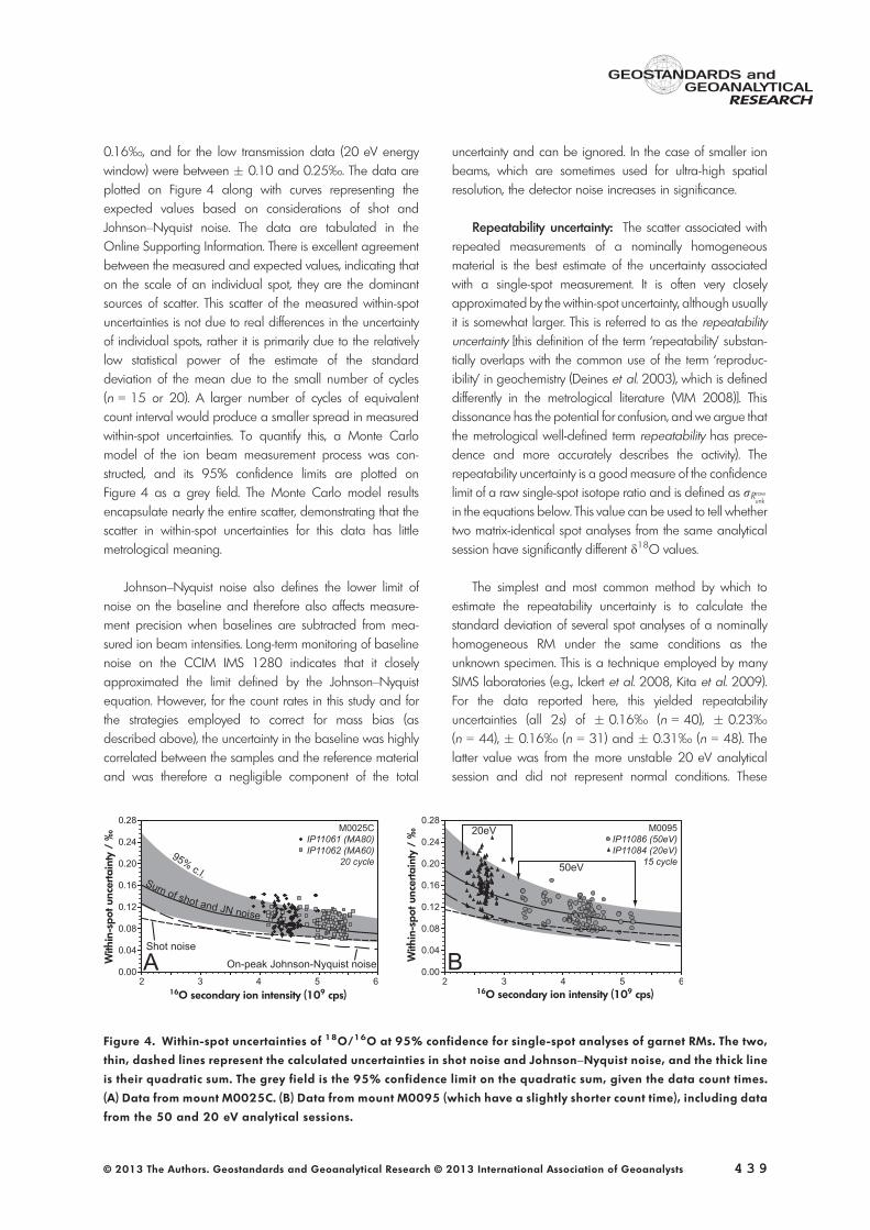
0.16‰, and for the low transmission data (20 eV energywindow) were between � 0.10 and 0.25‰. The data areplotted on Figure 4 along with curves representing theexpected values based on considerations of shot andJohnson–Nyquist noise. The data are tabulated in theOnline Supporting Information. There is excellent agreementbetween the measured and expected values, indicating thaton the scale of an individual spot, they are the dominantsources of scatter. This scatter of the measured within-spotuncertainties is not due to real differences in the uncertaintyof individual spots, rather it is primarily due to the relativelylow statistical power of the estimate of the standarddeviation of the mean due to the small number of cycles(n = 15 or 20). A larger number of cycles of equivalentcount interval would produce a smaller spread in measuredwithin-spot uncertainties. To quantify this, a Monte Carlomodel of the ion beam measurement process was con-structed, and its 95% confidence limits are plotted onFigure 4 as a grey field. The Monte Carlo model resultsencapsulate nearly the entire scatter, demonstrating that thescatter in within-spot uncertainties for this data has littlemetrological meaning.
Johnson–Nyquist noise also defines the lower limit ofnoise on the baseline and therefore also affects measure-ment precision when baselines are subtracted from mea-sured ion beam intensities. Long-term monitoring of baselinenoise on the CCIM IMS 1280 indicates that it closelyapproximated the limit defined by the Johnson–Nyquistequation. However, for the count rates in this study and forthe strategies employed to correct for mass bias (asdescribed above), the uncertainty in the baseline was highlycorrelated between the samples and the reference materialand was therefore a negligible component of the total
uncertainty and can be ignored. In the case of smaller ionbeams, which are sometimes used for ultra-high spatialresolution, the detector noise increases in significance.
Repeatability uncertainty: The scatter associated withrepeated measurements of a nominally homogeneousmaterial is the best estimate of the uncertainty associatedwith a single-spot measurement. It is often very closelyapproximated by the within-spot uncertainty, although usuallyit is somewhat larger. This is referred to as the repeatabilityuncertainty [this definition of the term ‘repeatability’ substan-tially overlaps with the common use of the term ‘reproduc-ibility’ in geochemistry (Deines et al. 2003), which is defineddifferently in the metrological literature (VIM 2008)]. Thisdissonance has the potential for confusion, and we argue thatthe metrological well-defined term repeatability has prece-dence and more accurately describes the activity). Therepeatability uncertainty is a good measure of the confidencelimit of a raw single-spot isotope ratio and is defined as rRraw
unk
in the equations below. This value can be used to tell whethertwo matrix-identical spot analyses from the same analyticalsession have significantly different d18O values.
The simplest and most common method by which toestimate the repeatability uncertainty is to calculate thestandard deviation of several spot analyses of a nominallyhomogeneous RM under the same conditions as theunknown specimen. This is a technique employed by manySIMS laboratories (e.g., Ickert et al. 2008, Kita et al. 2009).For the data reported here, this yielded repeatabilityuncertainties (all 2s) of � 0.16‰ (n = 40), � 0.23‰(n = 44), � 0.16‰ (n = 31) and � 0.31‰ (n = 48). Thelatter value was from the more unstable 20 eV analyticalsession and did not represent normal conditions. These
Figure 4. Within-spot uncertainties of 18O/16O at 95% confidence for single-spot analyses of garnet RMs. The two,
thin, dashed lines represent the calculated uncertainties in shot noise and Johnson–Nyquist noise, and the thick line
is their quadratic sum. The grey field is the 95% confidence limit on the quadratic sum, given the data count times.
(A) Data from mount M0025C. (B) Data from mount M0095 (which have a slightly shorter count time), including data
values are slightly larger than the average within-spotuncertainty and the theoretical uncertainties of � 0.08–0.12‰. This method of estimating repeatability uncertaintyrequires identical analytical conditions between RM and theanalyte and assumes that the uncertainty of each spot isidentical.
An alternative procedure, common in Pb/U SIMSanalyses, is to directly incorporate the within-spot uncertaintyinto the determination of repeatability uncertainty (e.g.,Ludwig 2008). Here, the repeatability uncertainty is assumedto be a combination of the measured within-spot uncertaintyand an unknown but constant excess uncertainty, which maybe zero or greater. This technique was used here tocalculate the repeatability uncertainty, and the values areshown in Table 2. Specifically, it used the algorithmdescribed by Ludwig (2009), using a maximum likelihoodmethod to determine the magnitude of the excess uncer-tainty, which in turn was added to the within-spot uncertaintyto arrive at the repeatability uncertainty. This is a moregeneral method than using the standard deviation, as it cantake into account variations in analysis uncertainty that areapparent in the within-spot uncertainty. However, in themajority of cases, including those presented here, thevariability in the within-spot uncertainty is not significant,and the two techniques produce effectively identical results.
IMF uncertainty: At a session-to-session level, theuncertainty of aUAG (the IMF determined relative to UAG)must be propagated onto individual spot analyses. Thisuncertainty is determined by the confidence limits of themean RrawUAG (i.e., rRrawUAG
) for an analytical session, that is, themain RM to which each session’s IMF is pinned. For theresults in this study, the uncertainty was small, between� 0.02 and 0.06‰ (Table 2), and had very little effect onthe overall uncertainty budget. This uncertainty componentwas important when comparing analyses from differentanalytical sessions (e.g., when aUAG varies) that used thesame RM. (e.g., Stern and Amelin 2003).
Anchor reference material uncertainty: The accuracyof a SIMS analysis is limited by that of the referencematerials, and this must be considered when comparingd18O values measured relative to different RMs. In the casewhere there is no matrix correction, or one where we anchora matrix calibration curve to a single RM, we are initiallyconcerned with the uncertainty in the reference value for thismaterial. Here we refer to this uncertainty as rRtUAG in theequations below (UAG is our anchor), and for this and otherRMs discussed here, our best estimates of their uncertaintiesare in Table 3. For a complex matrix calibration scheme, theuncertainties in bulk data of the anchor RM as well as the
others used to establish the scheme are important inuncertainty analysis of applying the matrix correction (seenext section).
Here, we assume that the RMs have been characterisedfor their degree of oxygen isotope homogeneity by bulk andmicrobeam methods and have a micrometre-scale variabil-ity that is less than can be detected by high-precisionmicrobeam analyses. Oxygen isotope ratios of silicateminerals are analysed by fluorination, whereby oxygen isquantitatively extracted from the silicate sample by heating itin a fluorine- or chlorine-rich atmosphere, after which it ispurified, usually converted to CO2 and analysed in a dual-inlet mass spectrometer (Clayton and Mayeda 1963). Thed18O value of the gas sample is determined by sample-standard bracketing with a reference gas, the composition ofwhich is determined separately by comparison with a RM.Many laboratories use laser-based heating methods (Sharp1990) which, relative to Ni-rod-bomb analyses, yields amore rapid throughput and enhanced repeatability (Valleyet al. 1995).
It is not common for laser fluorination laboratories toreport analyses of enough RMs such that the repeatabilityof individual measurements can be quantified. This makes itdifficult to quantitatively establish the precision of bulk d18Omeasurements. However, the repeatability of nominallyhomogeneous reference materials (measured by the stan-dard deviation of a large number of reference materials) iscommonly reported to be approximately � 0.2‰ (at 95%confidence). This repeatability value can be assessed inmore detail by examining the unusually large andcomprehensive data set of RM analyses that was publishedby Valley et al. (1995). In that paper, they reported d18Odata on UWG-2 garnet from 212 analytical sessions.Looking only at the final 94 sessions (for which therepeatability was clearly superior to the prior data,apparently due to technical improvements), and correctingthe reported standard deviations for sampling bias bymultiplying by a Student’s t factor, the mean repeatability forthese analyses is � 0.19‰ (very similar to the SIMS datain this study).
The uncertainty in the mean d18O value of bulk analysescan be decreased by n-0.5 through pooling multipleanalyses. At a repeatability of 0.19‰, four or more analysesneed to be pooled to achieve a precision better than 0.1‰.The precision cannot be improved infinitely, as at some levelinaccuracies and other systematic uncertainties becomeimportant. To a limited extent, the results of the UWG-2round robin among several laboratories reported by Valleyet al. (1995) can provide insight into the limit of precision.
Seven laboratories made multiple measurements of thed18O of UWG-2 several times (relative to NBS-28 quartzwith a consensus d18Ovsmow value of 9.59‰). The standarddeviation of these seven mean values is 0.078‰, yielding95% confidence limits of � 0.19‰. Taking these factors intoaccount, it is reasonable to expect that few reported bulkd18O values, either single or pooled results, will haveuncertainties better than 0.10‰ at 95% confidence. Thislower estimate is consistent with comprehensively reportedresults from laboratories doing high-precision laser fluorina-tion work (e.g., Cooper et al. 2009).
This analysis of the uncertainties relating to the bulk d18Omeasurements suggests that they are of the same order ofmagnitude as the repeatability of the SIMS data, andtherefore, they also need to be taken into account whendetermining an uncertainty on a single SIMS analysis.Nevertheless, the uncertainties relating to the bulk data aresystematic and should be ignored when comparing oxygenisotope analyses from the same session or from differentsessions using the same reference material, but they becomeimportant sources of uncertainty when comparing d18Oresults with either bulk analyses or analyses normalised to adifferent reference material.
There are other sources of uncertainty in calibration thatare beyond the scope of this paper, but are, nonetheless,worth noting. Many laser fluorination laboratories normalisesilicate data to UWG-2 garnet (Valley et al. 1995) with arecommended d18O value of 5.8‰ relative to VSMOW. Thisvalue, in turn, is normalised to a d18O value of NBS-28 of9.59‰. Unfortunately, the d18O value of NBS-28 relative toVSMOW is poorly known, with an uncertainty of � 0.2‰listed on the certificate of analysis (Hut 1987, Gonfiantiniet al. 1995, IAEA 2007). Sixteen average d18O determina-tions of NBS-28 are reported by the IAEA on the 2007certificate of analysis and yield an uncertainty of � 1.1‰(2s). Even after eliminating the two highest and two lowestanalyses, it is only reduced to � 0.6‰. Recent measure-ments of NBS-28 directly against VSMOW have yieldedd18O values that are 9.18‰, which is 0.41‰ lower than theconsensus value (Kusakabe and Matsuhisa 2008). Whilenot necessarily a problem for self-consistent silicate data sets,it is troubling that such an important measurement is sopoorly determined and makes comparison between silicateand other data sets, such as carbonate minerals, difficult.
Finally, the uncertainty in the isotope ratio of SMOW(which very closely approximates the 18O/16O of VSMOW)is only known to be � 0.22‰ (2s; Baertschi 1976),although only rarely is the actual isotope ratio, rather thanthe isotope delta value, of interest.
Matrix effect uncertainty: A more complex uncertaintycomponent is that associated with the correction for matrixeffects, ramatrix . Because there is no precise phenomenologicaldescription of SIMS matrix effects, the functional forms of therelationships between garnet chemistry (or crystal structure)and amatrix are unknown. Limited empirical evidence seemsto suggest that, for binary mixtures of end members of garnet(and other silicates), the amatrix is likely to be a smooth andmonotonic function of chemical composition and can besuccessfully modelled by degree one or two polynomials(Kita et al. 2007, 2010, Ickert et al. 2008, Page et al.2010).
Here, a second-degree polynomial was used to correctfor matrix effects in Ca–Mg–Fe garnets. A Monte Carlosimulation was employed to determine the parameters anduncertainties. For each iteration of the simulation, theindividual data points are perturbed within their expanded95% confidence limits (expanded by an excess scatter termto take into account scatter about the calibration that is notaccounted for by the measured 95% confidence limits oneach RM). The 95% confidence uncertainties of the calibra-tion of a garnet of independently known compositionranged from � 0.10 to 0.25‰ with a median value of0.20‰ (Figure 2). The uncertainties were lowest at XCa* ofthe UAG and increased at XCa* lower and higher,particularly the latter where the calibration was poorlyconstrained by RMs. To a good approximation, the � 95%confidence limits, in ‰, can be represented by a sixth-orderpolynomial as a function of XCa* ðP6
n¼0 CnXnCa�Þ, with
coefficients, C6 to C0, of 11.621, -36.305, +47.042, -32.19,+11.301, -1.4044 and +0.1536. The range of uncertaintiesis similar to the repeatability uncertainty and must be addedto the final uncertainty of any spot for which there is asignificant matrix correction.
Propagation: Using the first-term Taylor series expan-sion method for uncertainty propagation (e.g., de ForestPalmer 1912, Birge 1939, Ku 1966), the absolute uncer-tainty in Rtunk, denoted by rRt
unk, as a function of the
uncertainty due to repeatability ðrRrawunkÞ, the IMF correction
ðrRrawUAGÞ, the true value of the anchor RM ðrRtUAGÞ and the
matrix effect correction (ramatrix ), is as follows:
The data presented here are consistent with thesuggestion that the main source of matrix-related IMF isthe Ca abundance (Vielzeuf et al. 2005, Page et al. 2010).The relative abundances of Mg and Fe vary widely in thesegarnets and may also contribute to the IMF. To examine thispossibility, the residuals about the calibration curve for low-Ca RMs (with XCa* < 0.14, the XCa* of UAG) have beenplotted against Mg# in Figure 5. This figure shows whethera particular sample plots above or below the Ca calibrationcurve and whether that correlates with Mg/Fe. These RMshave a wide range of Mg# (Mg/(Fetot+Mg), from 0.25 to0.96, with very little Cr [maximum Cr# (Cr/Al + Cr) of 0.01].A linear regression of the data (Rock 1987, Helsel andHirsch 2002) yields a slope of 0.7+1.8-1.2 Mg#-1, which is withinuncertainty of zero. This suggests that any matrix effectassociated with Mg/Fe is not significant for these garnetsunder common analytical conditions.
Page et al. (2010) fit a Mn-rich garnet to their CaAl–CaCr calibration, however, from our analysis of our Mn-richRM (S0060, with XCa* = 0.03), the apparent measuredamatrix of -0.49 � 0.15‰ is outside of uncertainty of the-0.85 � 0.12‰ based upon the calibration at XCa* = 0.03.Given that there is no a priori reason to expect that a Mn-richgarnet behaves in a similar manner to a Mg–Fe-rich garnet,this suggests that it is not appropriate to use our scheme tonormalise garnets with a substantial Mn content.
The influence of Cr substitution on matrix effects isimportant for accurate analyses of mantle-derived Cr-richgarnet, which has a narrow range of Mg# and low XCa*(near 0.80 and less than 0.20, respectively; Schulze 2003).However, they have a relatively large range in Cr#, up to
0.50 (Stachel and Harris 2008). In principle, if Cr does notinfluence the mass bias, these samples can be analysedusing the Ca-based correction method.
When corrected using the method described above forXCa*, S0165 (Cr# = 0.15, XCa* = 0.13) yielded a d18Ovsmow
value of 5.60 � 0.44‰, nominally higher than the bulk d18Ovalue of 5.17 � 0.39‰, althoughboth estimates hada largeuncertainty due to the variability in the laser fluorinationmeasurements. S0113 (Cr# = 0.26, XCa* = 0.06) yielded ad18Ovsmow value of 6.12 � 0.23‰, substantially higher thanthe bulk value of 5.25 � 0.15‰ (Figure 5).
The Ca-corrected SIMS data for the high-Cr samples,when combined with UAG, yielded an apparent calibrationexcess of 0.34‰ per 0.1 Cr#. In principle, this could be usedas a second-order matrix correction; however, it is not knownhow the Ca-related matrix effect relates to a Cr-relatedmatrix effect: they could be linearly additive or complementeach other in a non-linear and unpredictable manner. Theeffect could also be non-linear. Given these uncertaintiesand the small number of RMs, it is clear that more work isrequired before matrix effects can be effectively corrected onCr-rich garnet.
Although our data did not show any evidence forsecondary matrix effects, this is not evidence for theirabsence. The data collected at a low band-pass (20 eV)showed enhanced matrix effects, i.e., higher or lower valuesrelative to UAG. These enhanced effects may be used toinfer the presence and magnitude of matrix effects at normaloperating conditions.
Figure 5. Testing the matrix effect of Mg# on garnet
O-isotope calibration. Shown is the co-variation of the
residual about the Ca garnet calibration (Figure 2) and
Mg# for low-Ca, Mg–Fe garnets. Although statistically
insignificant, the apparent slight positive correlation
The values of ematrix at 50 and 20 eV are plotted onFigure 6A. Most of the ematrix values at 20 eV are enhancedrelative to their 50 eV ematrix values – positive values arehigher and negative values are lower. For example,grossular and andradite garnets (which have a largecompositional difference from UAG and positive ematrix
values at 50 eV) have increases in ematrix in the range of0.8–1.0‰. In contrast, iron-rich, Ca-poor and Mn-richgarnets, which have negative ematrix values at 50 eV,showed small (~0.4‰), but significant decreases that fallbelow the unity line on the plot. The two Mg-rich, Ca-poorgarnets were exceptions to this trend.
Calcium-rich garnets with Ca abundances greater thanUAG exhibited a linear increase in matrix effects, consistentwith an overall enhancement of approximately +1‰ atXCa* = 1.0, i.e., a matrix correction of 4‰, rather than 3‰,as documented in the 50 eV data set (Figure 6B).
In Figure 6C, the difference between the Ca-correcteddata and the measured value (at 20 eV) is plotted againstMg#. The correlation between Mg# and the deviation fromthe (Ca-corrected) calibration is excellent. The enhancementfrom 0.2‰ to 0.8‰ at an Mg# of 0.96 is of the same orderof magnitude of that observed for Ca-rich garnets. Thesedata for the Ca-poor, Fe–Mg-rich garnets appear to amplifya secondary matrix effect associated with varying Mg/Fe,one that is only subtly present at 50 eV (Figure 5). Smallbiases may indeed be present in high-Mg/Fe or low-Mg/Fegarnet (when corrected based on Ca content) for typicaloperating conditions.
In contrast to the Ca-rich and Ca-poor garnets, the Cr-rich garnets did not show a systematic enhancement ofmatrix effects as the energy window was narrowed. Whencorrected in the usual way for Ca abundance, the deviationof the two Cr-rich RMs, previously +0.4‰ and 0.9‰ and50 eV, was +1.0‰ at 20 eV for both. This result highlightsour poor understanding of how matrix effects based onsingle chemical vectors interact – whether they sum in a linearmanner or whether they interact in a more complex way.
The technique of varying the energy bandwidth may beuseful in the early stages of a SIMS technique development, tohighlight or predict the direction and magnitude of matrixeffects and guide the development of reference material.Secondarily, this exercise illustrates once again and perhapsobviously that instrumental conditions can have a significanteffect, not only on the magnitude of IMF, but also on itssystematics. Additional experiments could have been done tovary instrument parameters: for example, the transfer magni-fication adjusted over a wider range than carried out here, the
entrance slit varied, the FA varied, etc. No matter howelaborate a particular matrix correction schemes becomes, inorder for it to have use beyond the individual laboratory, theeffects of the key instrumental parameters must be understoodto gauge its general utility. We emphasise this point due to thefact that the Cameca instrument designs allow, and indeedpromote, the customisation of operating conditions according
Figure 6. (A) Comparison of the secondary ion mass
spectrometry O-isotope data collected with 50 eV
energy window vs. 20 eV. Note the enhanced instru-
mental mass fractionation (IMF) for the 20 eV data. (B)
Variation in e matrix e = amatrix - 1 for the 20 eV data
plotted in an identical manner to Figure 2. (C) Residual
IMF vs. Mg# for 20 eV data set; see Figure 5 at 50 eV
to the desires of the analyst, often within a wide and ad hocoperational envelope. The fact that the amatrix values mea-sured here were virtually identical to the ones reported byPage et al. (2010) for the same instrument operated with ahigher transfer magnification of 2009 (MA40), and smallerFAs (4 mm) and energy slit (40 eV), suggests that there is goodlatitude for instrument parameters within the normal range ofoperation of the IMS 1280. It is wise practice, however, toassume that a matrix correction scheme is robust only for alimited range of instrument conditions, unless demonstratedotherwise.
Uncertainties
A typical uncertainty budget and the uncertainties onsingle-spot analyses are shown in Figure 7. Depicted aretwo end-member cases, with data typical for the analysespublished here. One has a relatively large uncertaintyassociated with repeatability (approximately � 0.3‰) anda large matrix effect correction, and the other has a smallrepeatability and a small matrix correction, effectivelyyielding maximum and minimum possible uncertainties.The analyses are arbitrarily centred at 0‰, and each point
Figure 7. Uncertainty budget for matrix-corrected, single-spot garnet secondary ion mass spectrometry d18O
analyses. The d18O uncertainties are drawn as 95% confidence limits on a hypothetical analysis yielding a mean
value of 0‰ . From left to right, they show the effect of the addition of each component of uncertainty. The addition of
the uncertainty in NBS-28 is shown for reference only, this uncertainty is systematic (almost perfectly correlated) for
silicate analyses that can be traced either to UWG-2 or NBS-28 or to both and is therefore usually neglected. The pie
charts illustrate the relative magnitudes of the variance (i.e., the squared values of the confidence limits) for different
uncertainty components and do not linearly scale to the contributions to the total uncertainty. The uncertainty in
d18ORM (bulk reference value of the reference material) was fixed at � 0.1‰, and the uncertainty in d18ONBS-28 was
� 0.2‰ (IAEA 2007). (A) The representative ‘worst’ case for this study, that is, the largest uncertainties for
repeatability, aUAG, and amatrix. (B) The best case for this study, that is, the smallest uncertainties for repeatability,
represents the effect of adding the additional components ofuncertainty.
When a single-spot analysis is to be compared withanother single-spot analysis of the same matrix during thesame analytical session, the uncertainty on that value can bebetter than � 0.2‰ (at 95% confidence). However, for thepurposes of comparing a matrix-corrected garnet d18Ovalue with an analysis of a different material, by a differenttechnique, the compounding effects of uncertainties in matrixeffect correction and uncertainties in reference materialcompositions can elevate the minimum uncertainty to� 0.3–0.4‰ (Figure 7). In particular, the effect of the matrixcorrection can be very large, especially for small repeat-ability uncertainties. These factors must be taken into accountwhen reporting or using high-precision SIMS d18O analyses.
These uncertainties cannot be eliminated, but some ofthem can be attenuated. First, the d18O value of NBS-28 isneedlessly imprecise, and this uncertainty extends to anyd18O value based upon it, such as the widely used UWG-2or the UAG RM introduced here. The development of aconsensus value with smaller and better constrained uncer-tainties is well within current analytical capabilities (e.g.,Kusakabe and Matsuhisa 2008) Second, although it doesnot seem likely that the precision of laser fluorinationanalyses will progress beyond the � 0.1‰ range, theassessment and reporting of uncertainties for these values isoften absent or difficult to decipher. In particular, anassessment on how well the difference in 18O/16O betweentwo silicate materials can be resolved on a session-to-sessionbasis within individual laboratories and between differentlaboratories is sorely lacking.
It is not likely that a useful phenomenology will bedeveloped soon for SIMS matrix effects. However, experi-ments with large numbers of well-characterised RMs thatpopulate simple binary or ternary mineral solid solutions,such as those presented in Page et al. (2010) and Vielzeufet al. (2005) and here, would provide a better understand-ing of (a) the general functional forms of the relationshipsbetween amatrix and matrix compositions; (b) the relation-ships between amatrix for different compositional variables(e.g., Do the amatrix values for different compositional vectorssum in a linear manner or do they interact in a morecomplex way?); (c) the uncertainties in these relationships;and (d) identification of key physical controls so that themagnitude and direction of IMF due to matrix effects can bepredicted.
A remaining problem is in the treatment of uncertaintiesin SIMS d18O values that represent aggregates (e.g., the
mean) of several spots. In principle, in taking the mean of anincreasing number of spots, the uncertainty reduces as n-0.5.This makes the assumption that: (a) the individual spots aresampling a population with a Gaussian distribution and (b)the population that is being sampled has a mean value thatis equivalent to the ‘true’ 18O/16O in the sample. The firstassumption can be justified in many cases. The secondassumption is more difficult to evaluate.
Conclusions
We have demonstrated that spot-to-spot precision for18O/16O on nominally homogeneous garnet grains can bebetter than � 0.2‰ at 95% confidence for high count ratemeasurements with dual Faraday cups. These uncertaintiesare very close to those expected by considerations of shotand Faraday detector noise.
On the CCIM IMS 1280, matrix effects associated with18O/16O measurements of Ca–Mg–Fe2+ garnet could beaccurately corrected by consideration of the relative Caabundance and the use of a robust, empirically determinedcalibration curve. Under typical operating conditions, theMg/Fe did not significantly affect the mass bias; however,the Ca-based correction alone cannot provide an accuratecorrection for garnet with substantial Mn and Cr. The Ca-related matrix effect was reproducible on different epoxymounts and at a range of operating conditions that aretypical of this model instrument; however, matrix effects wereamplified by strongly restricting the accepted range of ionenergies.
It is necessary to determine the uncertainties associatedwith IMF corrections. The uncertainties associated with matrixcorrections are relatively simple to derive and of similarmagnitude to the spot-to-spot uncertainty, about � 0.2‰.Uncertainties associated with bulk fluorination methods areprobably on the order of � 0.1‰ and provide a funda-mental constraint on the accuracy of SIMS results.
Acknowledgements
John Craven supplied many of the garnets in this studyand allowed the use of unpublished d18O data. TomChacko and Katie Smart supplied the UAG garnet sample.Andrew Locock supplied S0141 and S0142, and GrahamPearson supplied S0113. Gayle Hatchard is thanked forlaboratory assistance. Ilya Bindeman (University of Oregon)is thanked for supplying some of the laser fluorinationanalyses. Two anonymous reviewers for GGR are thankedfor comments that helped to clarify the paper, and JohnValley is thanked for comments on a previous version of the
manuscript. RBI was supported by a Killam PDF and by anNSERC Discovery grant to Thomas Stachel. This work relatesto CCIM Project P0010.
References
Akizuki M. (1989)Growth structure and crystal symmetry of grossular garnetsfrom the Jeffrey Mine, Asbestos, Quebec, Canada. Amer-ican Mineralogist, 74, 859–864.
Baertschi P. (1976)Absolute 18O content of standard mean ocean water.Earth and Planetary Science Letters, 31, 341–344.
Bartholom�e P. (1960)Genesis of the Gore Mountain garnet deposit, New York.Economic Geology, 55, 255–277.
Birge R.T. (1939)The propagation of errors. American Journal of Physics, 7,351–357.
de Chambost E., Fercocq P., Fernandes F., Deloule E. andChaussidon M. (1998)Testing the Cameca IMS1270 multicollector. In: Gillen, G.,Lareau, R., Bennett, J. & Stevie, F. (eds), Secondary IonMass Spectrometry, SIMS XI. Wiley (Orlando, Florida),727–730.
Chopin C. (1984)Coesite and pure pyrope in high-grade blueschists ofthe Western Alps: A first record and some consequences.Contributions to Mineralogy and Petrology, 86, 107–118.
Clayton R.N. and Mayeda T.K. (1963)The use of bromine pentafluoride in the extraction ofoxygen from oxides and silicates for isotopic analysis.Geochimica et Cosmochimica Acta, 27, 43–52.
Cooper K.M., Eiler J.M., Sims K.W.W. and Langmuir C.H.(2009)Distribution of recycled crust within the upper mantle:Insights from the oxygen isotope composition of MORBfrom the Australian-Antarctic Discordance. GeochemistryGeophysics Geosystems, 10, 26.
Coplen T.B. (2011)Guidelines and recommended terms for expression ofstable-isotope-ratio and gas-ratio measurement results.Rapid Communications in Mass Spectrometry, 25, 2538–2560.
Craig H. (1953)The geochemistry of the stable carbon isotopes. Geochi-mica et Cosmochimica Acta, 3, 53–92.
Deer W.A., Howie R.A. and Zussman J. (1982)Rock-forming minerals (2nd edition). Wiley (Bath).
Deines P., Goldstein S.L., Oelkers E.H., Rudnick R.L. andWalter L.M. (2003)Standards for publication of isotope ratio and chemicaldata in Chemical Geology. Chemical Geology, 202, 1–4.
Eiler J.M., Graham C. and Valley J.W. (1997)SIMS analysis of oxygen isotopes: Matrix effects in complexminerals and glasses. Chemical Geology, 138, 221–244.
Fitzsimons I.C.W., Harte B. and Clark R.M. (2000)SIMS stable isotope measurement: Counting statistics andanalytical precision. Mineralogical Magazine, 64, 59–83.
de Forest Palmer A. (1912)The theory of measurements. McGraw-Hill Book Company(New York).
Gnaser H. and Hutcheon I.D. (1987)Velocity-dependent isotope fractionation in secondary-ionemission. Physical Review B, 35, 877–879.
Gonfiantini R. (1978)Standards for stable isotope measurements in naturalcompounds. Nature, 271, 534–536.
Gonfiantini R., Stichler W. and Rozanski K. (1995)Standards and intercomparison materials distributed by theInternational Atomic Energy Agency for stable isotopeanalysis, Reference and intercomparison materials forstable isotopes of light elements. Proceedings of a consul-tants meeting held in Vienna, 1–3 December 1993.International Atomic Energy Agency (Vienna), 13–29.
Helsel D.R. and Hirsch R.M. (2002)Statistical methods in water resources. Techniques ofwater-resources investigations, Book 4, chapter A3, U.S.Geological Survey, 522pp.
Hervig R.L., Williams P., Thomas R.M., Schauer S.N. andSteele I.M. (1992)Microanalysis of oxygen isotopes in insulators by second-ary ion mass-spectrometry. International Journal of MassSpectrometry and Ion Processes, 120, 45–63.
Hut G. (1987)Stable isotope reference samples for geochemical andhydrological investigations. Report Consultants GroupMeeting. International Atomic Energy Agency (Vienna),42pp.
IAEA (2007)NBS 28 and NBS 30 reference sheet for referencematerials. IAEA (Vienna), 5pp.
Ickert R.B., Hiess J., Williams I.S., Holden P., Ireland T.R.,Lanc P., Schram N., Foster J.J. and Clement S.W.J. (2008)Determining high precision, in situ, oxygen isotope ratioswith a SHRIMP II: Analyses of MPI-DING silicate-glassreference materials and zircon from contrasting granites.Chemical Geology, 257, 114–128.
Jamtveit B. and Hervig R.L. (1994)Constraints on transport and kinetics in hydrothermal systemsfrom zoned garnet crystals. Science, 263, 505–508.
Johnson J.B. (1928)Thermal agitation of electricity in conductors. PhysicalReview, 32, 97–109.
Kita N.T., Ushikubo T., Fu B., Spicuzza M.J. and ValleyJ.W. (2007)Analytical developments on oxygen three isotope analysesusing a new generation ion microprobe ims-1280. Lunarand Planetary Science Conference abstract 1981.
Kita N.T., Ushikubo T., Fu B. and Valley J.W. (2009)High precision SIMS oxygen isotope analysis and the effectof sample topography. Chemical Geology, 264, 43–57.
Kita N.T., Nagahara H., Tachibana S., Tomomura S.,Spicuzza M.J., Fournelle J.H. and Valley J.W. (2010)High precision SIMS oxygen three isotope study ofchondrules in LL3 chondrites: Role of ambient gas duringchondrule formation. Geochimica et Cosmochimica Acta,74, 6610–6635.
Klein-BenDavid O. and Pearson D.G. (2009)Origins of subcalcic garnets and their relation to diamondforming fluids – Case studies from Ekati (NWT-Canada)and Murowa (Zimbabwe). Geochimica et CosmochimicaActa, 73, 837–855.
Ku H.H. (1966)Notes on the use of propagation of error formulas. Journalof Research of the National Bureau of Standards – C.Engineering and Instrumentation, 70C, 263–273.
Kusakabe M. and Matsuhisa Y. (2008)Oxygen three-isotope ratios of silicate reference materialsdetermined by direct comparison with VSMOW-oxygen.Geochemical Journal, 42, 309–317.
Locock A.J. (2008)An Excel spreadsheet to recast analyses of garnet into end-member components, and a synopsis of the crystalchemistry of natural silicate garnets. Computers andGeosciences, 34, 1769–1780.
Ludwig K.R. (2001)SQUID 1.02: A user’s manual. Berkeley GeochronologyCenter (Berkeley, CA). Special Publication No. 2.
Ludwig K.R. (2008)Isoplot 3.66 a geochronological toolkit for Microsoft Excel.Berkeley Geochronology Center (Berkeley, CA). SpecialPublication No. 4.
Ludwig K.R. (2009)SQUID2: A user’s manual, 2.5th edition. Berkeley Geo-chronology Center (Berkeley, CA), 100pp.
Migeon H.N., Schuhmacher M. and Slodzian G. (1990)Analysis of insulating specimens with the Cameca IMS4f.Surface and Interface Analysis, 16, 9–13.
Nyquist H. (1928)Thermal agitation of electric charge in conductors. PhysicalReview, 32, 110–113.
Page F.Z., Kita N.T. and Valley J.W. (2010)Ion microprobe analysis of oxygen isotopes in garnets ofcomplex chemistry. Chemical Geology, 270, 9–19.
Riciputi L.R., Paterson B.A. and Ripperdan R.L. (1998)Measurement of light stable isotope ratios by SIMS: Matrixeffects for oxygen, carbon, and sulfur isotopes in minerals.International Journal of Mass Spectrometry, 178, 81–112.
Rock N.M.S. (1987)Robust – an interactive Fortran-77 package for exploratorydata-analysis using parametric, robust and nonparametric
location and scale estimates, data transformations, nor-mality tests, and outlier assessment. Computers andGeosciences, 13, 463–494.
Russell W.A., Papanastassiou D.A. and Tombrello T.A.(1980)The fractionation of Ca isotopes by sputtering. RadiationEffects and Defects in Solids, 52, 41–52.
Schottky W. (1918)€Uber spontane Stromschwankungen in verschiedenenElektrizit€atsleitern. Annalen der Physik, 362, 541–567.
Schuhmacher M., Fernandes F. and de Chambost E.(2004)Achieving high reproducibility isotope ratios with theCameca IMS 1270 in the multicollection mode. AppliedSurface Science, 231–232, 878–882.
Schulze D.J. (2003)A classification scheme for mantle-derived garnets inkimberlite: A tool for investigating the mantle and exploringfor diamonds. Lithos, 71, 195–213.
Sharp Z.D. (1990)A laser-based microanalytical method for the in situdetermination of oxygen isotope ratios of silicates andoxides. Geochimica et Cosmochimica Acta, 54, 1353–1357.
Sharp Z.D., Essene E.J. and Hunziker J.C. (1993)Stable isotope geochemistry and phase equilibria ofcoesite-bearing whiteschists, Dora Maira Massif, westernAlps. Contributions to Mineralogy and Petrology, 114,1–12.
Slodzian G. (1975)Some problems encountered in secondary ion emissionapplied to elementary analysis. Surface Science, 48,161–186.
Slodzian G. (1980)Microanalyzers using secondary ion emission. Advances inElectronics and Electron Physics, Supplement, 13B, 1–44.
Slodzian G., Lorin J.C. and Havette A. (1980)Isotopic effect on the ionization probabilities in secondaryion emission. Journal de Physique – Lettres, 41, 555–558.
Slodzian G., Chaintreau M. and Dennebouy R. (1986)The emission objective lens working as an electron mirror:Self regulated potential at the surface of an insulatingsample. In: Benninghoven A., Colton R.J., Simons D.S. &Werner H.W. (eds), Secondary Ion Mass Spectrometry:SIMS V. Springer (Berlin), 158–160.
Smith D. and Boyd F.R. (1992)Compositional zonation in garnets in peridotite xenoliths.Contributions to Mineralogy and Petrology, 112,134–147.
Stachel T. and Harris J.W. (2008)The origin of cratonic diamonds – Constraints from mineralinclusions. Ore Geology Reviews, 34, 5–32.
Stern R.A. and Amelin Y. (2003)Assessment of errors in SIMS zircon U-Pb geochronologyusing a natural zircon standard and NIST SRM 610 glass.Chemical Geology, 197, 111–142.
Valley J.W., Kitchen N., Kohn M.J., Niendorf C.R. andSpicuzza M.J. (1995)UWG-2, a garnet standard for oxygen isotope ratios:Strategies for high precision and accuracy with laserheating. Geochimica et Cosmochimica Acta, 59, 5223–5231.
Vielzeuf D., Champenois M., Valley J.W., Brunet F. andDevidal J.L. (2005)SIMS analyses of oxygen isotopes: Matrix effects in Fe-Mg-Ca garnets. Chemical Geology, 223, 208–226.
VIM (2008)International Vocabulary of Metrology – Basic and generalconcepts and associated terms (VIM). Joint Committee forGuides in Metrology, Bureau International des Poids etMesures, 90pp.
Whitehouse M.J. and Nemchin A.A. (2009)High precision, high accuracy measurement of oxygenisotopes in a large lunar zircon by SIMS. ChemicalGeology, 261, 31–41.
Supporting information
Additional Supporting information may be found in theonline version of this article:
Table S1. Raw data for each spot analysis.
Table S2. Full data summary for each reference materialfor each analytical session.
This material is available as part of the online articlefrom: http://onlinelibrary.wiley.com/doi/10.1111/j.1751-908X.2013.00222.x/abstract (This link will take you to thearticle abstract).