Matrix-valued kernels for shape deformation analysisshape2015/slides/micheli.pdf · Mario Micheli...

Matrix-valued kernelsfor shape deformation analysis

Mario Micheli

University of San Francisco

Infinite-dimensional Riemannian geometry withapplications to image matching and shape analysis

Erwin Schrodinger International Institute for Mathematical Physics

January 16, 2015

Mario Micheli (USF) Matrix-valued kernels for shape deformation analysis

Summary of talk:

Motivation: shape spaces, LDDMM, manifold of landmarks

Metrics induced my Matrix-valued kernels

Examples

Reference:

MM, J Glaunes, Matrix-valued Kernels for Shape Deformation

Analysis. Geometry, Imaging, and Computing , 1(1):57-139, 2014.


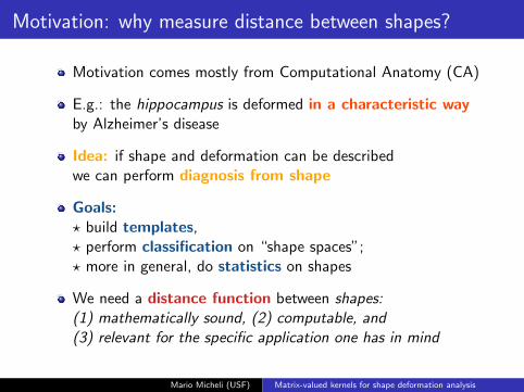
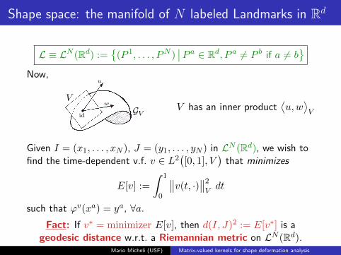
Motivation: why measure distance between shapes?

Motivation comes mostly from Computational Anatomy (CA)

E.g.: the hippocampus is deformed in a characteristic wayby Alzheimer’s disease

Idea: if shape and deformation can be describedwe can perform diagnosis from shape

Goals:? build templates,? perform classification on “shape spaces”;? more in general, do statistics on shapes

We need a distance function between shapes:(1) mathematically sound, (2) computable, and(3) relevant for the specific application one has in mind


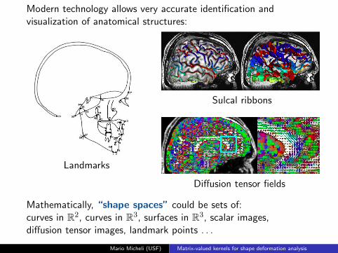
Modern technology allows very accurate identification andvisualization of anatomical structures:

Landmarks

Sulcal ribbons

Diffusion tensor fields

Mathematically, “shape spaces” could be sets of:curves in R2, curves in R3, surfaces in R3, scalar images,diffusion tensor images, landmark points . . .


Large Deformation Diffeomorphic Metric Mapping(LDDMM) – Trouve, Younes, Miller, Mumford, Michor. . .

ϕ ∈ Φ

Gid

ϕd

Φ

Idea: • Take a group of diffeomorphisms G, with Riemannian metric

Idea: • For two “shapes” S1 and S2 find subset of diffeos Φ ⊂ GIdea: • such that every ϕ ∈ Φ performs the matching S1 → S2

Idea: • Define

∫d(S1, S2) := inf

ϕ∈ΦdG(ϕ, id)

Idea: • This induces a Riemannian metric on the shape space


More details on LDDMM in Rd

V = Reproducing Kernel Hilbert Space of vector fields

E.g.: V = Hs(Rd,Rd), with s > d2 + 1.

This implies V ↪→ C10 (Rd,Rd); and V has a reproducing kernel .

In general, for v ∈ L2([0, 1], V ), we consider the ODE{∂ϕ∂t (t, x) = v

(t, ϕ(t, x)

)ϕ(0, x) = x

The solution ϕv(t, ·) is a diffeomorphism for all t ∈ [0, 1].

Define ϕv(·) = ϕv(1, ·). The set:

GV :={ϕv∣∣ v ∈ V }

is a group of diffeomorphisms (Trouve).


Shape space: the manifold of N labeled Landmarks in Rd

L ≡ LN (Rd) :={

(P 1, . . . , PN )∣∣P a ∈ Rd, P a 6= P b if a 6= b

}Now,

V

GVid

u

w V has an inner product⟨u,w

⟩V

Given I = (x1, . . . , xN ), J = (y1, . . . , yN ) in LN (Rd), we wish tofind the time-dependent v.f. v ∈ L2

([0, 1], V

)that minimizes

E[v] :=

∫ 1

0

∥∥v(t, ·)∥∥2

Vdt

such that ϕv(xa) = ya, ∀a.

Fact: If v∗ = minimizer E[v], then d(I, J)2 := E[v∗] is ageodesic distance w.r.t. a Riemannian metric on LN (Rd).


Landmark trajectories

We can track the trajectories of the N landmarks along theflow of v∗:

qa(t) := ϕv∗(t, xa), a = 1, . . . , N.

solutions to the ODEs

qa = v∗(t, qa)

qa(0) = xa, qa(1) = ya

a = 1, . . . , N

The N trajectories are a geodesic curve in LN (Rd)(w.r.t. the metric induced on LN (Rd) by the diffeo group)


Reproducing Kernel Hilbert Spaces (V, 〈·, ·〉V ) ofvector-valued functions Rd → Rd

∃! K : Rd × Rd → Rd×d, the reproducing kernel of V ,s.t. ∀x, α ∈ Rd⟨

K(·, x)α, u⟩V

= α · u(x), ∀u ∈ V.

Properties:

K(x, y) = K(y, x)T , for all x, y ∈ Rd

Positive definiteness:∀N ∈ N, x1, . . . , xN ∈ Rd, and α1, . . . , αN ∈ Rd,

N∑a,b=1

αa ·K(xa, xb)αb ≥ 0

with equality iff α1 = · · · = αN = 0.

uniqueness of reproducing kernels.


If we want to compute the geodesic connecting two points in LN (Rd),

the minimizer of E[v] =

∫ 1

0

∥∥v(t, ·)∥∥2

Vdt

has the form v∗(t, x) =

N∑a=1

K(x, qa(t)

)pa(t), pa = “momenta”

Scalar kernels: K(x, y) = k(‖x− y‖

)Id for some k : R+ → R.

K(x, 0)p1, p1 = (1, 0)∑3

a=1K(x, qa)pa


Scalar kernels: K(x, y) = k(‖x− y‖

)Id for some k : R+ → R.

Positive definiteness of K ⇐⇒ positive definiteness of k(‖ · ‖)

Theorem (Bochner)

A function f ∈ L1(Rd,R) is positive definite iff f := F [f ] ≥ 0.

We have F[k(‖ · ‖)

](‖ξ‖) = h(‖ξ‖), ξ ∈ Rd, with

h(%) :=2π

%µ

∫ ∞0

rµ+1k(r) Jµ(2π%r) dr , % > 0(

where µ =d

2−1)

• “Hankel Transform” H of order µ.

• K positive definite ⇔ h ≥ 0.


The Hankel Transform H is an involution (HH = Id), so

k(r) =2π

rµ

∫ ∞0

%µ+1h(%) Jµ(2π%r) d% , r > 0,

and generate admissible kernels from positive functions h.

Examples:

Gaussian kernels: k(r) = exp(− 1

2

r2

σ2

)Cauchy kernels: k(r) =

1

1 + x2/σ2

Bessel Kernels: k(r) =( rσ

)`− d2K`− d

2

( rσ

)


Translation- and Rotation-Invariant (TRI) kernels

We now consider matrix-valued kernels K : Rd × Rd → Rd×d.We want ‖ · ‖V to be invariant under translation & rotation:

v1 v2 v3

We want:

‖v1‖V = ‖v2‖V = ‖v3‖V

Properties of K?


Elementary Linear Algebra: Projection Operators in Rd

α‖ = Pr‖x α

x ∈ Rd \ {0}

Pr‖x :=xxT

‖x‖2eig(Pr‖x) = 1 (multiplicity 1) and 0 (multiplicity d− 1)

Pr⊥x := Id −xxT

‖x‖2eig(Pr⊥x ) = 0 (multiplicity 1) and 1 (multiplicity d− 1)

M := aPr‖x + bPr⊥xxxT

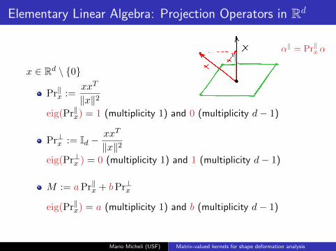
‖x‖2eig(Pr‖x) = a (multiplicity 1) and b (multiplicity d− 1)


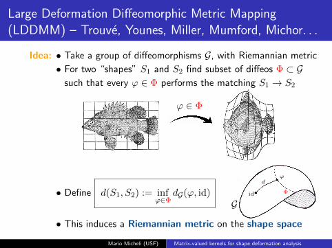
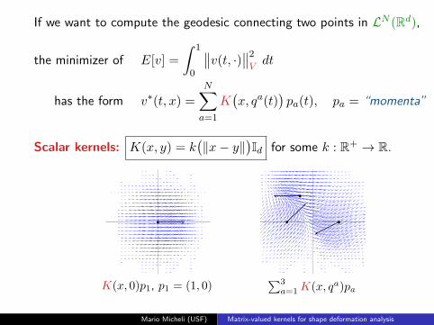
General form of TRI kernels

Theorem

If ‖ · ‖V is translation- and rotation-invariant then its kernel hasthe form

K(x, y) = k(x− y)

withk(x) = k‖(‖x‖) Pr‖x + k⊥(‖x‖) Pr⊥x

for some functions k‖, k⊥ : R+ → R, scalar valued.

Remark 1: k‖(‖x‖), k⊥(‖x‖) are the eigenvalues of k(x)

Reminder: in the scalar case k(x) = k(‖x‖)Id.

Remark 2:when k‖ = k⊥ =: k we are in the scalar case (Pr

‖x+Pr⊥x =Id)


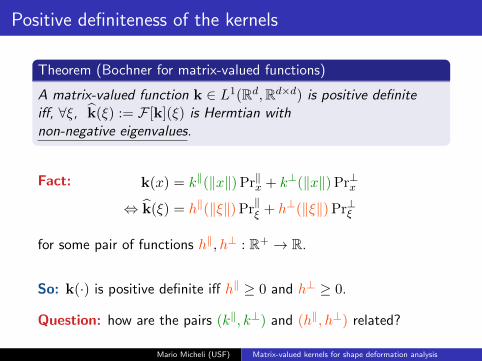
Positive definiteness of the kernels

Theorem (Bochner for matrix-valued functions)

A matrix-valued function k ∈ L1(Rd,Rd×d) is positive definiteiff, ∀ξ, k(ξ) := F [k](ξ) is Hermtian withnon-negative eigenvalues.

Fact: k(x) = k‖(‖x‖) Pr‖x + k⊥(‖x‖) Pr⊥x

⇔ k(ξ) = h‖(‖ξ‖) Pr‖ξ + h⊥(‖ξ‖) Pr⊥ξ

for some pair of functions h‖, h⊥ : R+ → R.

So: k(·) is positive definite iff h‖ ≥ 0 and h⊥ ≥ 0.

Question: how are the pairs (k‖, k⊥) and (h‖, h⊥) related?


“Generalized” Hankel Transform

The map T : (k‖, k⊥) 7→ (h‖, h⊥) is given by:

h‖(%) =2π

%µ

∫ ∞0

rµ+1 k‖(r)Jµ(2π%r) dr

− 2µ+ 1

%µ+1

∫ ∞0

rµ(k‖(r)− k⊥(r)

)Jµ+1(2π%r) dr.

h⊥(%) =2π

%µ

∫ ∞0

rµ+1 k⊥(r)Jµ(2π%r) dr

+1

%µ+1

∫ ∞0

rµ(k‖(r)− k⊥(r)

)Jµ+1(2π%r) dr.

where µ := d2 − 1

Remark:

• condition for positive definiteness of k: h‖ ≥ 0 and h⊥ ≥ 0

• when k‖ = k⊥ we retrieve the usual Hankel transform


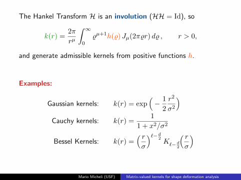
Fact: the Generalized Hankel Transform T is an involution,i.e. T−1 = T

so T−1 : (h‖, h⊥) 7→ (k‖, k⊥) is given by:

k‖(r) =2π

rµ

∫ ∞0

%µ+1 h‖(%)Jµ(2πr%) d%

− 2µ+ 1

rµ+1

∫ ∞0

%µ(h‖(%)− h⊥(%)

)Jµ+1(2πr%) d%.

k⊥(r) =2π

rµ

∫ ∞0

%µ+1 h⊥(%)Jµ(2πr%) d%

+1

rµ+1

∫ ∞0

%µ(h‖(%)− h⊥(%)

)Jµ+1(2πr%) d%.

where µ :=d

2− 1

Remark:

• such formulas can be used to build functions k‖, k⊥

starting from non-negative h‖, h⊥ (generalizes [Schonberg 1938])


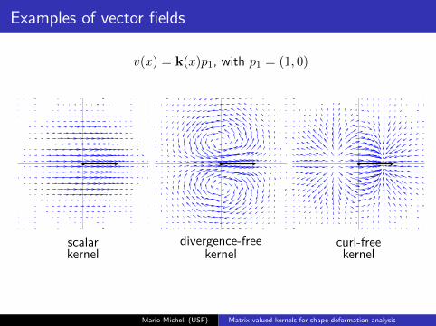
Main result: meaning of h‖ and h⊥

k(x) = k‖(‖x‖) Pr‖x + k⊥(‖x‖) Pr⊥x

k(ξ) = h‖(‖ξ‖) Pr‖ξ + h⊥(‖ξ‖) Pr⊥ξ

F

Properties of the vector fields in the RKSH V :

Condition on (h‖, h⊥)

divergence-free h‖ = 0

curl-free h⊥ = 0

Remark 1: (h‖, h⊥) correspond to the Hodge decomposition of v.f.’s.Remark 2: provides a technique to build div-free and curl free kernels.


Examples of vector fields

scalarkernel

divergence-freekernel

curl-freekernel

v(x) = k(x)p1, with p1 = (1, 0)


Examples of vector fields

scalarkernel

divergence-freekernel

curl-freekernel

v(x) =

3∑a=1

k(x− qa)pa


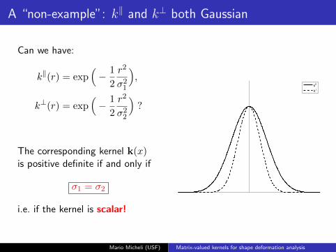
A “non-example”: k‖ and k⊥ both Gaussian

Can we have:

k‖(r) = exp(− 1

2

r2

σ21

),

k⊥(r) = exp(− 1

2

r2

σ22

)?

The corresponding kernel k(x)is positive definite if and only if

σ1 = σ2

i.e. if the kernel is scalar!

k||

k!


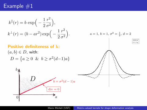
Example #1

k‖(r) = b exp(− 1

2

r2

σ2

),

k⊥(r) = (b− ar2) exp(− 1

2

r2

σ2

).

Positive definiteness of k:(a, b) ∈ D, with:

D ={a ≥ 0 & b ≥ σ2(d−1)a}

a

b

0

D b = σ2(d− 1)a

@Idiv = 0

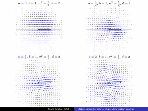
a = 1, b = 1, σ2 = 12, d = 2

k||

k!


a = 0, b = 1, σ2 = 12, d = 2

a = 32, b = 1, σ2 = 1

2, d = 2

a = 12, b = 1, σ2 = 1

2, d = 2

a = 2, b = 1, σ2 = 12, d = 2


Example #2

k‖(r) = (b− ar2) exp(− 1

2

r2

σ2

),

k⊥(r) = b exp(− 1

2

r2

σ2

).

Positive definiteness of k:(a, b) ∈ D, with:

D ={a ≥ 0 & b ≥ σ2a}

a

b

0

Db = σ2a

@Icurl = 0

a = 1, b = 1, σ2 = 12, d = 2

k||

k!


a = 0, b = 1, σ2 = 12, d = 2

a = 32, b = 1, σ2 = 1

2, d = 2

a = 12, b = 1, σ2 = 1

2, d = 2

a = 2, b = 1, σ2 = 12, d = 2


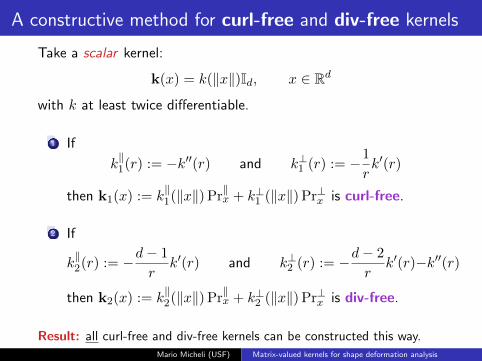
A constructive method for curl-free and div-free kernels

Take a scalar kernel:

k(x) = k(‖x‖)Id, x ∈ Rd

with k at least twice differentiable.

1 If

k‖1(r) := −k′′(r) and k⊥1 (r) := −1

rk′(r)

then k1(x) := k‖1(‖x‖) Pr

‖x + k⊥1 (‖x‖) Pr⊥x is curl-free.

2 If

k‖2(r) := −d− 1

rk′(r) and k⊥2 (r) := −d− 2

rk′(r)−k′′(r)

then k2(x) := k‖2(‖x‖) Pr

‖x + k⊥2 (‖x‖) Pr⊥x is div-free.

Result: all curl-free and div-free kernels can be constructed this way.


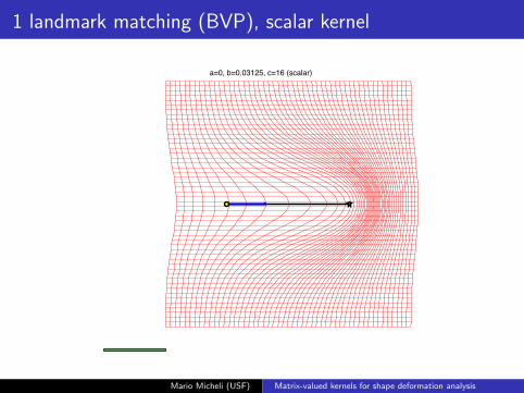
1 landmark matching (BVP), scalar kernel

a=0, b=0.03125, c=16 (scalar)


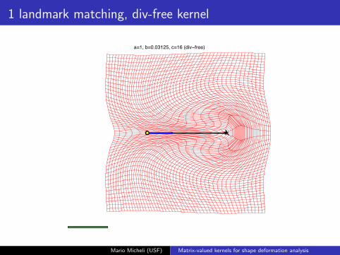
1 landmark matching, div-free kernel

a=1, b=0.03125, c=16 (div free)


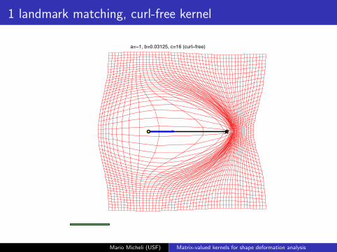
1 landmark matching, curl-free kernel

a= 1, b=0.03125, c=16 (curl free)


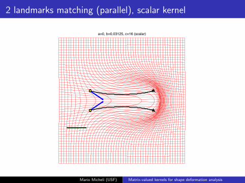
2 landmarks matching (parallel), scalar kernel

a=0, b=0.03125, c=16 (scalar)


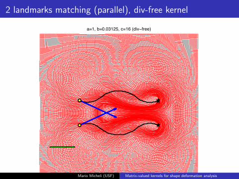
2 landmarks matching (parallel), div-free kernel

a=1, b=0.03125, c=16 (div free)


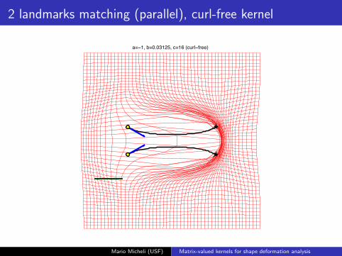
2 landmarks matching (parallel), curl-free kernel

a= 1, b=0.03125, c=16 (curl free)


2 landmarks matching (opposite), scalar kernel

a=0, b=0.03125, c=16 (scalar)


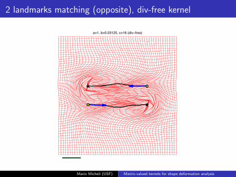
2 landmarks matching (opposite), div-free kernel

a=1, b=0.03125, c=16 (div free)


2 landmarks matching (opposite), curl-free kernel

a= 1, b=0.03125, c=16 (curl free)


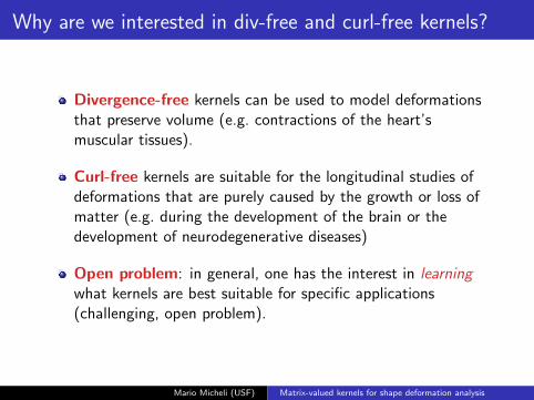
Why are we interested in div-free and curl-free kernels?

Divergence-free kernels can be used to model deformationsthat preserve volume (e.g. contractions of the heart’smuscular tissues).

Curl-free kernels are suitable for the longitudinal studies ofdeformations that are purely caused by the growth or loss ofmatter (e.g. during the development of the brain or thedevelopment of neurodegenerative diseases)

Open problem: in general, one has the interest in learningwhat kernels are best suitable for specific applications(challenging, open problem).


Thank you for listening!


Date post:	14-Mar-2020
Category:	Documents
Upload:	others
View:	13 times
Download:	0 times

Matrix-valued kernels for shape deformation analysisshape2015/slides/micheli.pdf · Mario Micheli...

Documents