MAVEN Contamination Venting and Outgassing Analysis Elaine M. Petro, David W. Hughes, MarkS. Secunda, Philip T. Chen, James R. Morrissey National Aeronautics and Space Administration/Goddard Space Flight Center, Greenbelt, MD 20771 and Catherine A. Riegle Lockheed Martin, Denver, CO, 80125 ABSTRACT Mars Atmosphere and Volatile EvolutioN (MA VE:I'I') is the frrst mission to focus its study on the Mars upper atmosphere. MAVEN will study the evolution ofthe Mars atmosphere and climate, by examining the conduit through which the atmosphere has to pass as it is lost to the upper atmosphere. An analysis was performed for the MAVEN mission to address two distinct concerns. The first goal of the analysis was to perform an outgassing study to determine where species outgassed from spacecraft materials would redistribute to and how much of the released material might accumulate on sensitive surfaces. The second portion ofthe analysis serves to predict what effect, if any, Mars atmospheric gases trapped within the spacecraft could have on instrument measurements when re-released through vents. The re-release of atmospheric gases is of interest to this mission because vented gases from a higher pressure spacecraft interior could bias instrument measurements ofthe Mars atmosphere depending on the flow rates and directions. ACRONYMS APP: Articulated Payload Platform CAD: Computer Aided Design EUV: Extreme UltraViolet GSFC: Goddard Space Flight Center HGA: High Gain Antenna IUVS: Imaging UltraViolet Spectrograph LGA: Low Gain Antenna LPW: Langmuir Probe and Waves MAG: Magnetometer MASTRAM: MASs TRansport Analysis Module MAYEN: Mars Atmosphere and Volatile EvolutioN MLI: Multi-Layer Insulation MSFC: Marshall Space Flight Center NASA: K ational Aeronautics and Space Administration NGIMS: Neutral Gas and Ion Mass Spectrometer OGR: Outgassing Rate RSDPU: Remote Sensing Data Processing Unit S: Sticking Coefficient S/C: Spacecraft SEP: Solar Energetic Particles STATIC: SupraThermal And Thermal Ion Composition SWEA: Solar Wind Electron Analyzer 1 SWIA: Solar Wind Ion Analyzer TQCM: Temperature-controlled Quartz Crystal Microbalance l.JV: Ultra-Violet MAVEN MISSON The Mars Atmosphere and Volatile EvolutioN (MAYEN) spacecraft (S/C) is a Mars orbiter, managed by National Aeronautics and Space Administration/Goddard Space Flight Center (NASNGSFC) and scheduled to launch in November 2013 and arrive at Mars orbit in August 2014. MA YEN will study the evolution of the Mars atmosphere over time and provide answers to questions about its climate history. Figure 1 shows the diverse instrument suite on board the spacecraft to make these measurements, which includes a quadrapole mass spectrometer (NGIMS), a Ultra- Violet (UV) image spectrometer (IUVS), a host of ion analyzing instruments (SWIA, SWEA, STATIC, SEP), a Langmuir probe (LPW), a magnetometer (MAG), and a solar irradiance sensor (EUV). . ' ' . '""" .,.. ._ h '1•'11t;. t•f .. ' ,_... .. - ' - ... , .... ... . .... .. , ... , ..... _, ... . ,- . ":. • • ._.I •, •• (L· :. ... "--" . .. . - ..., • t""z"• ,._- "·U• • : .. : ....... :.. .. # Figure 1 MAYEN Spacecraft and Instruments MAVEN will enter into an elliptical orbit around Mars with a nominal periapsis altitude of 150 km, which occasionally will decrease to 125 km for specific science-driven maneuvers (referred to as "Deep Dips"). For this study, the altitudes between 125 and 500 km are of the greatest interest. The analysis discussed in this paper was performed https://ntrs.nasa.gov/search.jsp?R=20160010595 2018-05-19T12:31:54+00:00Z
Transcript
MAVEN Contamination Venting and Outgassing Analysis
Elaine M. Petro, David W. Hughes, MarkS. Secunda, Philip T. Chen, James R. Morrissey National Aeronautics and Space Administration/Goddard Space Flight Center, Greenbelt, MD 20771
and
Catherine A. Riegle Lockheed Martin, Denver, CO, 80125
ABSTRACT
Mars Atmosphere and Volatile EvolutioN (MA VE:I'I') is the frrst mission to focus its study on the Mars upper atmosphere. MAVEN will study the evolution ofthe Mars atmosphere and climate, by examining the conduit through which the atmosphere has to pass as it is lost to the upper atmosphere.
An analysis was performed for the MAVEN mission to address two distinct concerns. The first goal of the analysis was to perform an outgassing study to determine where species outgassed from spacecraft materials would redistribute to and how much of the released material might accumulate on sensitive surfaces. The second portion ofthe analysis serves to predict what effect, if any, Mars atmospheric gases trapped within the spacecraft could have on instrument measurements when re-released through vents. The re-release of atmospheric gases is of interest to this mission because vented gases from a higher pressure spacecraft interior could bias instrument measurements ofthe Mars atmosphere depending on the flow rates and directions.
ACRONYMS
APP: Articulated Payload Platform CAD: Computer Aided Design EUV: Extreme UltraViolet GSFC: Goddard Space Flight Center HGA: High Gain Antenna IUVS: Imaging UltraViolet Spectrograph LGA: Low Gain Antenna LPW: Langmuir Probe and Waves MAG: Magnetometer MASTRAM: MASs TRansport Analysis Module MA YEN: Mars Atmosphere and Volatile EvolutioN MLI: Multi-Layer Insulation MSFC: Marshall Space Flight Center NASA: K ational Aeronautics and Space Administration NGIMS: Neutral Gas and Ion Mass Spectrometer OGR: Outgassing Rate RSDPU: Remote Sensing Data Processing Unit S: Sticking Coefficient S/C: Spacecraft SEP: Solar Energetic Particles STATIC: SupraThermal And Thermal Ion Composition SWEA: Solar Wind Electron Analyzer
1
SWIA: Solar Wind Ion Analyzer TQCM: Temperature-controlled Quartz Crystal
Microbalance l.JV: Ultra-Violet
MAVEN MISSON
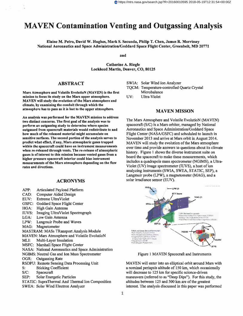
The Mars Atmosphere and Volatile EvolutioN (MA YEN) spacecraft (S/C) is a Mars orbiter, managed by National Aeronautics and Space Administration/Goddard Space Flight Center (NASNGSFC) and scheduled to launch in November 2013 and arrive at Mars orbit in August 2014. MA YEN will study the evolution of the Mars atmosphere over time and provide answers to questions about its climate history. Figure 1 shows the diverse instrument suite on board the spacecraft to make these measurements, which includes a quadrapole mass spectrometer (NGIMS), a UltraViolet (UV) image spectrometer (IUVS), a host of ion analyzing instruments (SWIA, SWEA, STATIC, SEP), a Langmuir probe (LPW), a magnetometer (MAG), and a solar irradiance sensor (EUV).
MAVEN will enter into an elliptical orbit around Mars with a nominal periapsis altitude of 150 km, which occasionally will decrease to 125 km for specific science-driven maneuvers (referred to as "Deep Dips"). For this study, the altitudes between 125 and 500 km are of the greatest interest. The analysis discussed in this paper was performed
in effort to estimate and compare the flow magnitudes and directions ofboth 'natural' Mars gases and 'unnatural' gases released from the spacecraft as MAVEN transits its orbit. The ultimate goal is to ensure that each of the instrument payloads on the MAVEN spacecraft is able to meet its science measurement requirements without interference or bias from the spacecraft itself
INTRODUCTION
An analysis was performed for the MAVEN mission to address two distinct concerns. The frrst goal of the analysis was to perform an outgassing study to determine where species outgassed from spacecraft materials would redistribute to and how much of the released material might accumulate on sensitive surfaces. The second portion of the analysis serves to predict what effect, if any, that atmospheric gases trapped within the spacecraft could have on instrument measurements when re-released through vents. The re-release of atmospheric gases is of interest to this mission because vented gases from a higher pressure spacecraft interior could bias instrument measurements of the Martian atmosphere depending on the flow rates and directions.
Thus the frrst portion of the analysis deals with the redistribution of non-native ( outgassed) species that are released from spacecraft materials and the second portion addresses the redistribution of native Martian (atmospheric) species absorbed and re-released through venting as MAVEN transits its orbit.
ANALYSIS SETUP
A 3D geometrical model of the MAVEN spacecraft was developed using NX/Ideas. This model was based on a top level mechanical spacecraft model that was provided by the MAVEN project. An additional thermal engineering Computer Aided Design (CAD) model was referenced for Multi-Layer Insulation (MLI) design.
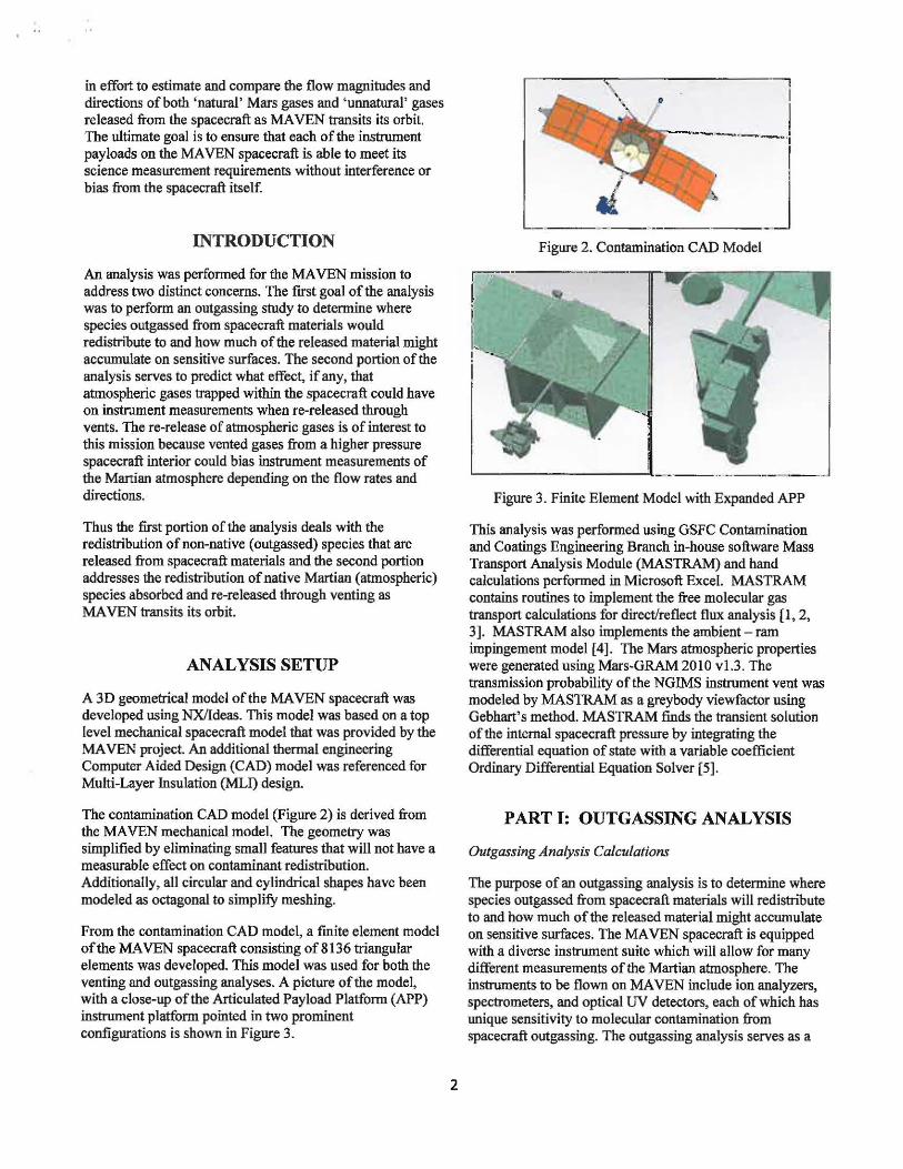
The contamination CAD model (Figure 2) is derived from the MAVEN mechanical model. The geometry was simplified by eliminating small features that will not have a measurable effect on contaminant redistribution. Additionally, all circular and cylindrical shapes have been modeled as octagonal to simplify meshing.
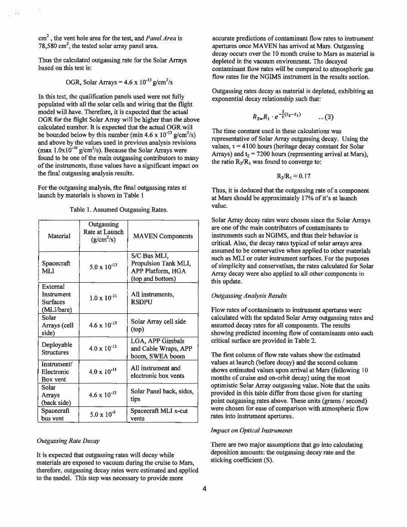
From the contamination CAD model, a fmite element model of the MAVEN spacecraft consisting of 8136 triangular elements was developed. This model was used for both the venting and outgassing analyses. A picture of the model, with a close-up of the Articulated Payload Platform (APP) instrument platform pointed in two prominent configurations is shown in Figure 3.
2
.--------..----------·-r I
I . ------~
/ J -~--------Figure 2. Contamination CAD Model
L...----------4- ----- - -------·-~-
Figure 3. Finite Element Model with Expanded APP
This analysis was performed using GSFC Contamination and Coatings Engineering Branch in-house software Mass Transport Analysis Module (MASTRAM) and hand calculations performed in Microsoft Excel. MAS TRAM contains routines to implement the free molecular gas transport calculations for direct/reflect flux analysis [ 1, 2, 3]. MAS TRAM also implements the ambient - ram impingement model [4] . The Mars atmospheric properties were generated using Mars-GRAM 2010 vl.3. The transmission probability of the NGIMS instrument vent was modeled by MASTRAM as a greybody viewfactor using Gebhart's method. MASTRAM finds the transient solution of the internal spacecraft pressure by integrating the differential equation of state with a variable coefficient Ordinary Differential Equation Solver [5].
PART 1: OUTGASSING ANALYSIS
Outgassing Analysis Calculations
The purpose of an outgassing analysis is to determine where species outgassed from spacecraft materials will redistribute to and how much of the released material might accumulate on sensitive surfaces. The MAVEN spacecraft is equipped with a diverse instrument suite which will allow for many different measurements of the Martian atmosphere. The instruments to be flown on MAVEN include ion analyzers, spectrometers, and optical UV detectors, each of which has unique sensitivity to molecular contamination from spacecraft outgassing. The outgassing analysis serves as a
tool to determine which components may pose the greatest threat to instrument measurements.
At first cut, the outgassing analysis was performed in a format that assigned characteristic outgassing rates (OGRs) to elements based on components and materials. Using these emission rates, molecular transport calculations were employed to determine the total amount of outgassed material that might impinge on instrument apertures. While this method is useful for identifying the combined outgassing threat to instrument apertures, it proves to be a tedious framework for evaluating the viability of different combinations of outgassing rates from different components. (Achievable component specific outgassing rates may change throughout the integration and testing process due to careful material usage, bakeout durations and temperatures, changes in requirements, etc.).
Thus the outgassing analysis framework was subsequently restructured such that it is based on view factors to critical surfaces. For example, the view factor between an instrument aperture and the spacecraft MLI indicates what fraction of the material outgassed from the spacecraft MLI will reach the instrument aperture. Thus an appropriate outgassing rate for the source material (i.e. MLI) can be determined from the instrument's sensitivity requirement. Through this format, a system of equations is developed that relates each instrument's sensitivity requirement, the view factors to outgassing sources, and the outgassing rates of the sources. The outgassing budget can thus be refmed by solving the system of equations for outgassing rates that will satisfy the instrument sensitivity requirements. This approach is not fundamentally different from that of the first analysis, but just allows for greater flexibility in outgassing rate assignment.
Below is an example outgassing equation showing how the total flux to the instrument aperture is calculated for NGIMS, where cP is the flux of outgassed species in units of [g/cm2/s] , Area is the surface area, and Viewfactor is the greybody radiation view factor between the critical surface and each source. There is an analogous equation for each critical surface.
,~,1. = L.f ( 0t x Area1 x View[actor1 ) 'P ••. (1)
Areai
At this point, the system of equations has not been constrained by instrument sensitivity requirements to solve for appropriate outgassing rates. Instead, the flux to instrument apertures was again determined by assigning typical outgassing rates based on the source material. However, if it is found later that a source deviates significantly from its projected outgassing rate or that an instrument needs more stringent contamination requirements, the system of equations can be used to determine the impact and update the budget to account for the change.
3
Outgassing Analysis Inputs
An outgassing rate was supplied by the spacecraft provider for the MLI blankets. All other outgassing rates were unknown at the point the analysis was initiated and were therefore assumed for this analysis. The rates assumed were based generic material properties and outgassing rates typical of other NASA/GSFC missions. Rates were further refined as more material data became available for the MAVEN project. Different rates were applied to different segments of the spacecraft based on the assumed materials only and are not assumed to be temperature dependent at this point.
Outgassing rates were applied to the external surface elements only. Thus self-contamination from internal instrument surfaces was not considered in this analysis. The analysis does however take into account the redistribution of internal species that are released through instrument vents. Outgassed species were represented as generic hydrocarbons with a molecular weight of 300 glmol.
View factors between outgassing sources and critical surfaces were computed using the finite element model with the APP platform in the Fly-Y I Ram-Nadir configuration. View factors from this configuration were used in outgassing calculations, as this is assumed to be the predominant configuration during periapse passes. The periapse pass portion of the orbit occurs below 500 km, where the atmosphere is most dense and the most critical atmospheric measurements are performed.
Solar Array Outgassing Calculations
The assumed outgassing rates remained unchanged throughout the analysis iterations for all components except for the Solar Arrays. The outgassing rates for the Solar Arrays were updated to incorporate data collected during thermal vacuum testing of a Solar Array qualification panel in September 20 11 .
A revised Solar Array outgassing rate was implemented in the analysis following thermal vacuum testing and bakeout of a qualification panel. During this test, an MLI enclosure was used to heat the Solar Array to 105 degrees Celsius. A Temperature-controlled Quartz Crystal Microbalance (TQCM) inserted through the enclosure collected material at l 0 degrees Celsius.
The TQCM data, along with details about the enclosure and component geometry were used to estimate an outgassing rate for the Solar Arrays using the following equation:
Vent Area OGR = f.{ X STQCM X Panel Area ... (2)
Where STQCM is 1.97 x l o-9 glcm2/Hz, the mass sensitivity of a 15 MHz TQCM, LJf is 2566 Hzlhour, the measured rate of frequency change of the TQCM, Vent Area is given as 25.8
cm2 , the vent hole area for the test, and Panel Area is
78,580 cm2, the tested solar array panel area.
Thus the calculated outgassing rate for the Solar Arrays based ori this test is:
OGR, Solar Arrays= 4.6 x 10' 13 glcm2/s
In this test, the qualification panels used were not fully populated with all the solar cells and wiring that the flight model will have. Therefore, it is expected that the actual OGR for the flight Solar Array will be higher than the above calculated number. It is expected that the actual OGR will be bounded below by this number (min 4.6 x 10"13 g/cm%) and above by the values used in previous analysis revisions (max l.Ox10"10 glcm2/s). Because the Solar Arrays were found to be one of the main outgassing contributors to many of the instruments, these values have a significant impact on the final outgassing analysis results.
For the outgassing analysis, the final outgassing rates at launch by materials is shown in Table 1
Table 1. Assumed Outgassing Rates.
l Outgassing
Material Rate at Launch
MA YEN Components (glcm2/s)
S/CBusMLI, Spacecraft
5.0 X 10"13 i Propulsion Tank MLI,
I ML! ! I .AJ>P Platform, HG.A. I (top and bottom)
External ! Instrument 1.0 X 10"11 ! All instruments, Surfaces RSDPU
; (MLI/bare) Solar ! Solar Array cell side Arrays (cell ! 4.6 X 10'13
(top) side)
Deployable LGA, APP Gimbals
4.0 X 10-ll and Cable Wraps, APP Structures
boom, SWEA boom Instrument/
All instrument and Electronic 4.0 X 10"11
Box vent electronic box vents
Solar Solar Panel back, sides,
Arrays 4.6 X 10'13
(back side) tips
Spacecraft j 5.0 X 10"9 Spacecraft MLI x-cut
bus vent vents
Outgassing Rate Decay
It is expected that outgassing rates will decay while materials are exposed to vacuum during the cruise to Mars, therefore, outgassing decay rates were estimated and applied to the model. This step was necessary to provide more
4
accurate predictions of contaminant flow rates to instrument apertures once MA YEN has arrived at Mars. Outgassing decay occurs over the 1 0 month cruise to Mars as material is depleted in the vacuum environment. The decayed contaminant flow rates will be compared to atmospheric gas flow rates for the NGIMS instrument in the results section.
Outgassing rates decay as material is depleted, exhibiting an exponential decay relationship such that:
... (3)
The time constant used in these calculations was representative of Solar Array outgassing decay. Using the values, 1: = 4100 hours (heritage decay constant for Solar Arrays) and t2 = 7200 hours (representing arrival at Mars), the ratio R21R, was found to converge to:
Thus, it is deduced that the outgassing rate of a component at Mars should be approximately 17% ofit's at launch value.
Solar Array decay rates were chosen since the Solar Arrays are one of the main contributors of contaminants to instruments such as NGIMS, and thus their behavior is critical. Also, the decay rates typical of solar arrays area assumed to be conservative when applied to other materials such as MLI or outer instrument surfaces. For the purposes of simplicity and conservatism, the rates calculated for Solar Array decay were also applied to all other components in this update.
Outgassing Analysis Results
Flow rates of contaminants to instrument apertures were calculated with the updated Solar Array outgassing rates and assumed decay rates for all components. The results showing predicted incoming flow of contaminants onto each critical surface are provided in Table 2.
The ftrst column of flow rate values show the estimated values at launch (before decay) and the second column shows estimated values upon arrival at Mars (following I 0 months of cruise and on-orbit decay) using the most optimistic Solar Array outgassing value. Note that the units provided in this table differ from those given for starting point outgassing rates above. These units (grams I second) were chosen for ease of comparison with atmospheric flow rates into instrument apertures.
Impact on Optical instruments
There are two major assumptions that go into calculating deposition amounts: the outgassing decay rate and the sticking coefficient (S).
The sticking coefficient represents the fraction of the mass that reaches the surface that actually deposits. The sticking coefficient is strongly temperature dependent and precise optical temperatures are not yet known. Thus to bound the problem, deposition levels are given for two sticking coefficients: S = 1 (cold optic, maximum deposition) and S= 0.01 (warm optic, minimal deposition). The outgassing rates used in these calculations are the rates estimated for arrival at Mars. Further outgassing decay is not currently modeled
Table 2. Predicted Incoming Flow of Contaminants
Critical Incoming Flow of Primary
Surface Contaminants Contributing
(gls) Source(s)
At Launch At Mars
IUVSLimb 1.2 X 10"10 2.0 x to·11 self (next is APP A rture ' Platform IUVSNadir 5.2 X JO- IS 8.8 X )0"16 self (next is A erture RSDPU
Solar Arrays
NGIMS ! (next are APP
7.4 x w - IJ 1.3 x w -13 Boom I Platform I Aperture Components and I SEP)
self(next are STATIC 6.2 x w-Jc 1.0 x w-10 APPBoom/ Aperture Platform
' I Components)
' self(next are Aft SWEA 6.9 X 10-IG 1.2 x w -lo Electronics Aperture Boxes and
SWEAboom)
SWIA 2.9 X 10"10 4.9 x 10"11 , self(next is
Aperture · Spacecraft Bus
MLI and vents)
' HGA(bottom EUV I 1.9 X 10"11 3.3 X 10"12 . side) and
I Aperture · Spacecraft Bus
MLI SEP Aperture 5.4 X 10-l l 9.2 X 10"12 HGA(bottom
J+Y) side) SEP Aperture 5.o x ta-u 8.5 x w-12 HGA(bottom (-Y) side)
MAG(+Y) 3.4 X 10"11 5.7 X 10"12 Solar Arrays (tips)
MAG (-Y) 3.3 x w-11 5.6 x w-12 Solar Arrays (tips)
The IUVS and EUV instruments both contain internal optical surfaces that are sensitive to the deposition of molecular contaminants. Updated estimates of the deposition of contaminants over the 1 year mission life are presented in Table 3 for both instruments.
It is critical to note that the view factors used in this analysis are for the ram-nadir, Fly-Y, positioning of the APP platform and do not consider other pointing modes. The
5
view factors to the IUVS aperture would likely be increased in other pointing modes. The analysis also only considers impingement from external sources and does not account for self -contamination from internal surfaces. Thus, these values are presented as a preliminary point of evaluation and by no means are fmal.
Also, the view factors used in this analysis are to the instrument apertures, and not the optical surfaces, which results in values that are higher than what would actually reach the internal optics.
1 year science 1 year science Cruise+ (A) (A) Science (A)
IUVS scan 151 1.5 50
mirror EUV
internal 944 9.44 50 optics
Impact on Non-Optical Instruments
For reference, the flux of outgassed contaminants to instrument apertures is compared to the flux of atmospheric species for the non-optical and non-magnetic instruments. Table 4 shows the fluxes of contaminants at the beginning of on orbit operations and the atmospheric fluxes reported at two altitudes (150 km and 500 km). Atmospheric fluxes are greater at lower altitudes due to increased atmospheric density and higher spacecraft velocities.
This comparison of contaminant to atmospheric flux is most useful for the NGIMS instrument as it will be mapping the composition of the Martian atmosphere and thus will need to be able to distinguish native species from contaminants.
The ratio of contaminant to atmospheric flux is less important for the ion analyzers {STATIC, SWEA, and SWIA) and the SEP instrument as the fluxes reported in this analysis are only for neutral species. It is possible that contaminants on the sun-side of the spacecraft could become photo-ionized and thus could have an impact on these instruments. However, further investigation would be required to estimate the probability that photo-ionization would occur, and if so, what percent of the contaminants might become ionized and reach the apertures.
Outgassing Analysis Conclusions
Outgassing fluxes to instrument surfaces were estimated based on spacecraft material and relative orientation between components. These rates were then compared to the
target measurements for the instruments to evaluate their impact.
In order to evaluate the impact that these assumed outgassing rates could have on optical instrument measurements, an attempt was made to estimate the deposition on the surface. A very preliminary analysis indicates that the EUV and JUVS optical surfaces could see a large range of deposition during science operations based on what assumptions are made. Further work will be done to refine these assumptions based on optical temperatures, outgassing decay, and conductance through instrument apertures.
Table 4 . Outgassing versus Atmospheric Fluxes.
Incoming Incoming Incoming
Critical Flow of Flow of Flow of
Surface Contaminants Atmospheric Atmospheric -at Mars Gas -150 km Gas- 500 km (gls) (gls) (gls)
NGIMS 1.3 X 10·13 6.2 X 10'7 2.1 x 10"12
Aperture STATIC
1.0 X 10'10 5.4 X 10~ 2.0x 10⁻¹¹
Aperture SWEA '
Aperture 1.2 X 10' 10 5.3 X 10"6 2.0 x to-11
SWJA I 4.9 X 10'11 5.o x w·7 4.2 X 10"!2
Aperture SEP i Aperture 9.2 x 10"12 8.4 x w-7 2.9 x w-12
J.+Y) SEP Aperture I 8.5 X 10'12 5.8 X 10'7 2.0 x w-12
(-Y) I
For the non-optical instruments, contaminant fluxes were compare.d to atmospheric fluxes for two altitudes at the beginning of on orbit operations. It was found that the flux of contaminants is lower than the atmospheric species below 500 km. For NGIMS, the difference is between 1 and 2 orders of magnitude at 500 km, largely dependent on the Solar Array outgassing rate.
Similarly, the Solar Arrays were found to be the major contributing source for several instruments, including NGIMS, the ion analyzers (SWEA, SWIA, STATIC), and MAG. The HGA (specifically the bottom side) is a major contributing source to the SEP and EUV instruments, due to the close proximity and good views. Thus, if the flux values are too high for any of the inst:nmlents, the HGA and Solar Arrays would be the frrst place to start further investigation.
Part II: VENTING ANALYSIS
Venting Analysis Introduction
6
As MAVEN travels through its orbit, vents in the spacecraft MLI allow the inner bus volume to fill with molecules. Almost immediately, the inner volume becomes pressurized to at least one order of magnitude greater than the ambient atmosphere and then retains this pressure differential throughout the course of the orbit. This pressure differential leads to a constant flux of gas from the side and aft facing vents on the bus. The possibility of these sources biasing instrument measurements was studied.
This initial venting analysis assumed that there would be 24 x-cuts evenly distributed about the X andY faces of the spacecraft bus. The assumed cut width was 1116". Free molecular flow conductance properties were calculated for this vent geometry. The venting conductance was then combined with the calculated surface pressures and vent to instrument finite element method view factors to produce the final results. The calculations are discussed in some detail below.
Atmospheric and Surface Pressure Calculations
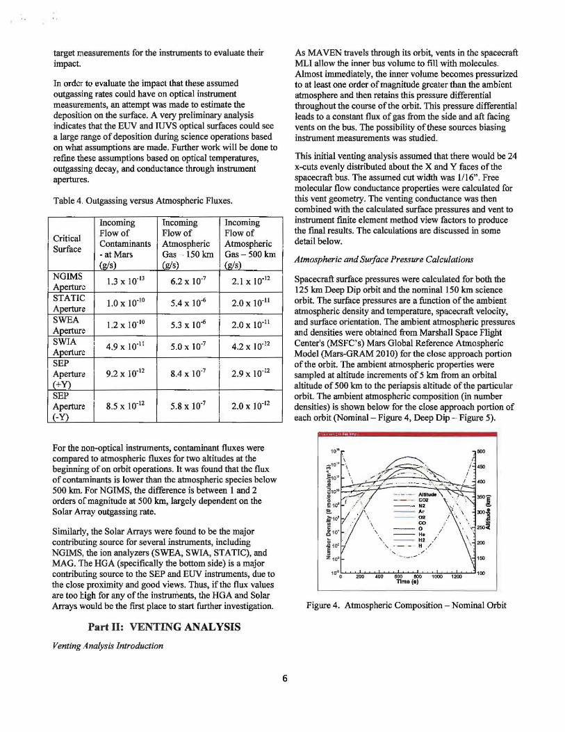
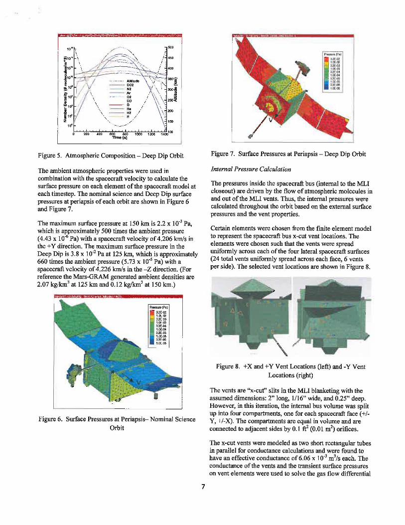
Spacecraft surface pressures were calculated for both the 125 km Deep Dip orbit and the nominal150 km science orbit. The surface pressures are a function of the ambient atmospheric density and temperature, spacecraft velocity, and surface orientation. The ambient atmospheric pressures and densities were obtained from Marshall Space Flight Center's (MSFC's) Mars Global Reference Atmospheric Model (Mars-GRAM 2010) for the close approach portion of the orbit. The ambient atmospheric properties were sampled at altitude increments of 5 km from an orbital altitude of 500 km to the periapsis altitude of the particular orbit. The ambient atmospheric composition (in number densities) is shown below for the close approach portion of each orbit (Nominal - Figure 4, Deep Dip - Figure 5).
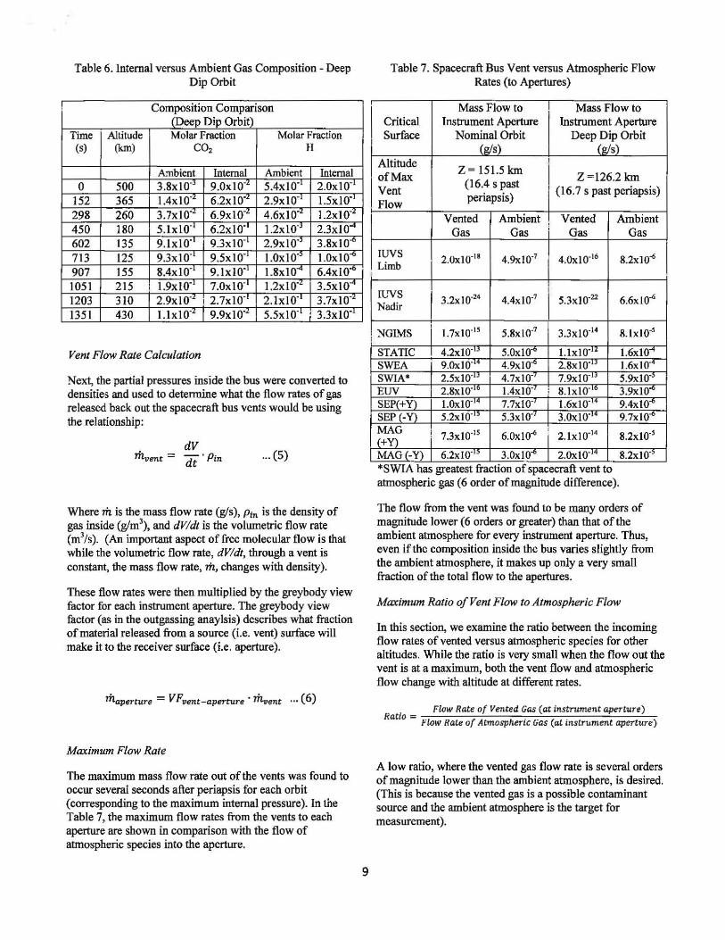
The ambient atmospheric properties were used in combination with the spacecraft velocity to calculate the surface pressure on each element of the spacecraft model at each timestep. The nominal science and Deep Dip surface pressures at periapsis of each orbit are shown in Figure 6 and Figure 7.
The maximum surface pressure at 150 krn is 2.2 x 10·3 Pa, which is approximately 500 times the ambient pressure (4.43 x 10-{) Pa) with a spacecraft velocity of 4.206 km/s in the + Y direction. The maximum surface pressure in the Deep Dip is 3.8 X 10"2 Pa at 125 km, which is approximately 660 times the ambient pressure (5.73 x 10"5 Pa) with a spacecraft velocity of 4.226 krn/s in the -Z direction. (For reference the Mars-GRAM generated ambient densities are 2.07 kg/km3 at 125 krn and 0.12 kglkrn3 at 150 krn.)
p.....,.(Pa)
~ 32E-112 IIIII! UE-111
32E-OO L HE-00 1:1 32E-1>4 I!J 1.oE-1>4
-~~:: 32E.OO I.OE-015
Figure 6. Surface Pressures at Periapsis- Nominal Science
Orbit
7
Figure 7. Surface Pressures at Periapsis - Deep Dip Orbit
Internal Pressure Calculation
The pressures inside the spacecraft bus (internal to the MLI closeout) are driven by the flow of atmospheric molecules in and out of the MLI vents. Thus, the internal pressures were calculated throughout the orbit based on the external surface pressures and the vent properties.
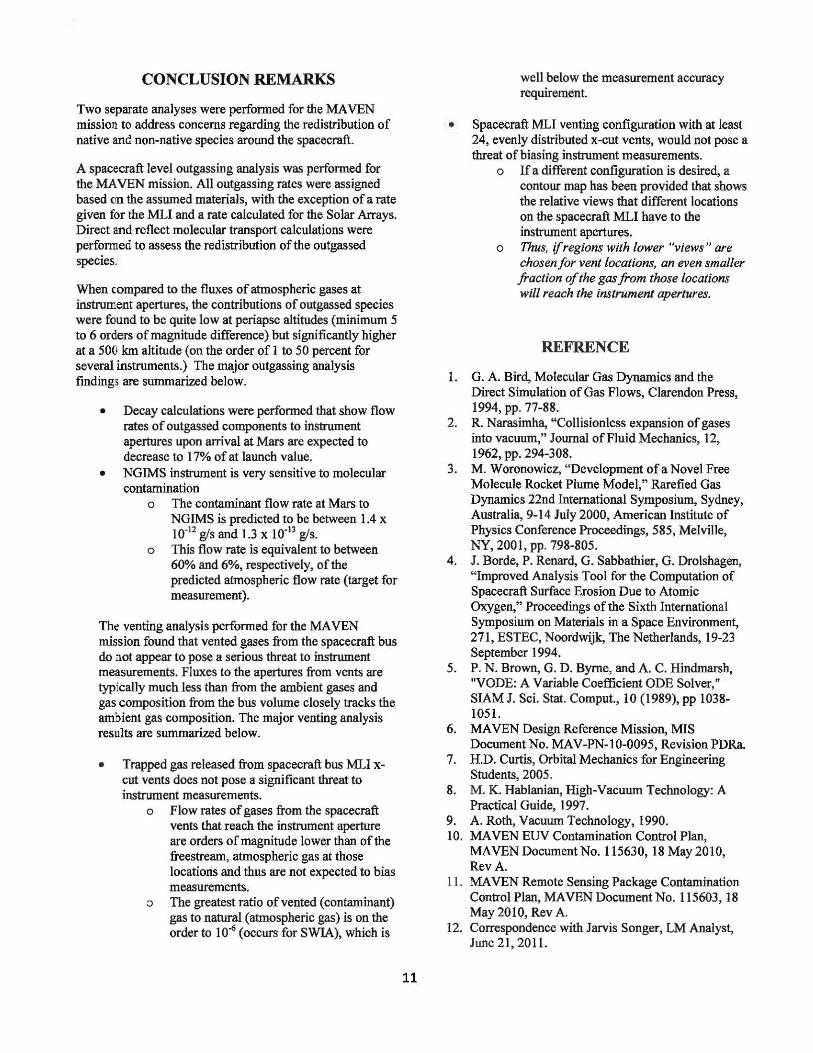
Certain elements were chosen from the finite element model to represent the spacecraft bus x-cut vent locations. The elements were chosen such that the vents were spread uniformly across each ofthe four lateral spacecraft surfaces (24 total vents uniformly spread across each face, 6 vents per side). The selected vent locations are shown in Figure 8.
Figure 8. +X and +Y Vent Locations (left) and-Y Vent
Locations (right)
The vents are ''x-cut" slits in the MLI blanketing with the assumed dimensions: 2" long, 1/16" wide, and 0.25" deep. However, in this iteration, the internal bus volume was split up into four compartments, one for each spacecraft face(+/Y, +/-X). The compartments are equal in volume and are connected to adjacent sides by 0.1 ~ (0.0 1 m2
) orifices.
The x-cut vents were modeled as two short rectangular tubes in parallel for conductance calculations and were found to have an effective conductance of 6.06 x 10"3 m3 /s each. The conductance of the vents and the transient surface pressures on vent elements were used to solve the gas flow differential
equation, giving the transient pressures inside the spacecraft bus:
dP V dt = C (LlP) ... (4)
where Vis the internal volume, dP/dt represents the internal pressure change rate, C is the vent conductance, and LlP is the pressure difference across the vent.
The differential equation was solved independently for each species so that the composition inside the spacecraft bus could be closely tracked. This method is appropriate for a molecular flow regime where the flow of molecules is dominated by interactions with the vessel surface instead of intermolecular collisions.
The pressures inside each cavity (inside the MLI close-out) are shown on the next page, first for the nominal science orbit (Figure 9) and then for the Deep Dip orbit (Figure 10). For reference, the pressures on two vents (one from the ram + Y face and one from the wake - Y face) and the ambient pressure are also shown. It can be seen in the plots that the internal pressure peaks slightly (about 16 seconds) after the orbit periapsis.
The lag between the internal and external pressure is due the time it takes for the pressure to equalize across the vents. It can also be seen from these results that the internal pressure remains higher than the ambient atmospheric pressures throughout most of the orbit, yet lower than the pressure on the ram face. This relationship can be seen in Figure 9 by comparing the internal and ram vent pressures. There are no vents on the ram face for the Deep Dip orbit (due to the change in pointing), but for reference, the ram pressure at periapsis is 3.8 x 10'2 Pa, as mentioned before, and thus is higher than the internal pressure.
Since the flow of each species was tracked independently, it is possible to compare the composition of gas inside the spacecraft bus to the ambient atmospheric gas. It was hypothesized that there could be a difference in composition because each species has a different density profile and travels at a different thermal velocity.
Tables 5 and 6 show the molar fraction of two different species (C02, highest molecular weight, and H, lowest molecular weight) for the gas internal to the bus and for the ambient gas at several time steps throughout the orbits. The molar fraction ofH increases with altitude, since it dominates the upper atmosphere. The molar fraction of C02
displays the opposite trend, since it dominates the lower atmosphere and then decays quickly with altitude.
Table 5. Internal versus Ambient Gas CompositionNominal Science Orbit
Composition Comparison (Nominal Science Orbit)
Time Altitude Molar Fraction Molar Fraction (s) (km) col H
Next, the partial pressures inside the bus were converted to densities and used to determine what the flow rates of gas released back out the spacecraft bus vents would be using the relationship:
dV ril.,ent = dt · Pin ... (5)
Where m is the mass flow rate (gls), Ptn is the density of gas inside (glm\ and dV/dt is the volumetric flow rate (m3/s). (An important aspect of free molecular flow is that while the volumetric flow rate, dV/dt, through a vent is constant, the mass flow rate, m, changes with density).
These flow rates were then multiplied by the greybody view factor for each instrument aperture. The greybody view factor (as in the outgassing anaylsis) describes what fraction of material released from a source (i.e. vent) surface will make it to the receiver surface (i.e. aperture).
'l'haperture = VFvent-aperture • ril.,ent ... (6)
Maximum Flow Rate
The maximum mass flow rate out of the vents was found to occur several seconds after periapsis for each orbit (corresponding to the maximum internal pressure). In the Table 7, the maximum flow rates from the vents to each aperture are shown in comparison with the flow of atmospheric species into the aperture.
9
Table 7. Spacecraft Bus Vent versus Atmospheric Flow Rates (to Apertures)
Mass Flow to Mass Flow to Critical Instrument Aperture Instrument Aperture Surface Nominal Orbit Deep Dip Orbit
(+Y) i MAG (-Y) 6.2xl0"15 3.0xl0·6 2.0x10⁻¹⁴ 8.2xto-s *SWIA has greatest fractton of spacecraft vent to atmospheric gas (6 order of magnitude difference).
The flow from the vent was found to be many orders of magnitude lower (6 orders or greater) than that of the ambient atmosphere for every instrument aperture. Thus, even if the composition inside the bus varies slightly from the ambient atmosphere, it makes up only a very small fraction of the total flow to the apertures.
Maximum Ratio of Vent Flaw to Atmospheric Flow
In this section, we examine the ratio between the incoming flow rates of vented versus atmospheric species for other altitudes. While the ratio is very small when the flow out the vent is at a maximum, both the vent flow and atmospheric flow change with altitude at different rates.
• ----:-F_l-:ow:--R_at-:e-:o:....f _v_en_te~d:::..:G:..:as~( a:::..:t-7-in:::..:s:..:.tr:..:u:::..:m.::e..:.n:::..:t a:!:p:..:.e:....:rt.::u:....:re::..).....,... Ratro = -:: Flow Rate of Atmospheric Gas (at instrument aperture)
A low ratio, where the vented gas flow rate is several orders of magnitude lower than the ambient atmosphere, is desired. (This is because the vented gas is a possible contaminant source and the ambient atmosphere is the target for measurement).
Shown in Figure 11 is a plot of both the atmospheric mass flow and the mass flow of gas from the vents into the NGIMS aperture throughout the close approach portion of the nominal orbit. Also shown on the graph, in green and on the second Y -axis, is the ratio between the amount of gas from the spacecraft vents to the amount of ambient gas at the NGIMS aperture.
Flow Comparison- NGI MS Aperture
1.0~<00 1.0£.()8
l.0[-01 ... 1.0[·().4 \ :!!
~~ ~ 1.0£·00
, · : .-- ·· · -~ l.0£·011 &
UlE·lO .r'·:""· / h "' ~ ~~ .. -··p l .OE-()9 :!'~ Ul£·12
! l.ot:-14 ia 8 G
~ 1.0E·16 /" .. " .5~
1.0£-18 ..... 1.0E·l0 r ........... l.OE·2l 1.0E·10
It can be seen from the plot that although the maximum flow out of the vent occurs just after periapsis (about 16 seconds past periapsis ), the ratio peaks slightly later when the spacecraft is at an outbound altitude of about 210 km (about 280 seconds past periapsis).
In Table 8, the maximum ratio of vented gas mass flow to atmospheric gas mass flow is shown for each critical surface. As stated above, this ratio is at a maximum at 21 0 km outbound.
Table 8 . Maximum Ratio of Vented to Ambient Gas (210 km, outbound)
R . fM Fl atlo o ass ows to Critical Surface Surface
(Vented I Atmospheric) IUVS Limb Aperture 8.7 X 10-t.:
' IUVS Nadir Aperture i 1.5 x 10⁻¹'
NGillS Aperture 7.4 X 10"" STATIC Aperture 2.1 X 10"7
SWEA Aperture 4.7 X 10-a SWIA Aperture* 1.2x 10⁻⁶ EUV Aperture 4.5 X 10·Y
SEP Aperture ( + Y) 3.4 X 10"11
SEP Aperture (-Y) 2.5 x to·a MAG (+Y) 3.0 X 10·"' MAG (-Y) 5.3 x 10-~
*SWIA again has greatest fraction of spacecraft vent to atmospheric gas (approx. I part per million by mass).
10
Venting Analysis Conclusions
An analysis was performed to determine if atmospheric gas vented from the spacecraft bus MLI vents could adversely impact instrument measurements. For the chosen vent scheme (24 vents, 6 evenly distributed across each face), the results of the analysis indicate that spacecraft bus venting of atmospheric gas does not pose any significant threat to instrument measurements. Even in the worst case, the contribution of vented gas is found to be 1 part per million or less of the total flow to an instrument aperture (SWIA specifically).
The exact locations of the spacecraft bus vents could be decided based on the contour map of the spacecraft by view factor to instrument apertures as shown in Figures 12 and 13. Thus, when choosing vent locations, it would be advisable to choose regions with lower views of instrument apertures (i.e. contoured green or blue) where possible.
Figure 12. View Factor Contour(+ X, +Y sides)
Figure 13. View Factor Contour (-X, -Y sides)
CONCLUSION REMARKS
Two separate analyses were performed for the MAVEN mission to address concerns regarding the redistribution of native and non-native species around the spacecraft.
A spacecraft level outgassing analysis was performed for the MAVEN mission. All outgassing rates were assigned based on the assumed materials, with the exception of a rate given for the MLI and a rate calculated for the Solar Arrays. Direct and reflect molecular transport calculations were performed to assess the redistribution of the outgassed species.
When compared to the fluxes of atmospheric gases at instrument apertures, the contributions of outgassed species were found to be quite low at periapse altitudes (minimum 5 to 6 orders of magnitude difference) but significantly higher at a 500 km altitude (on the order of 1 to 50 percent for several instruments.) The major outgassing analysis findings are summarized below.
• Decay calculations were performed that show flow rates of outgassed components to instrument apertures upon arrival at Mars are expected to decrease to 17% of at launch value.
• NGIMS instrument is very sensitive to molecular contamination
o The contaminant flow rate at Mars to NGIMS is predicted to be between 1.4 x 10"12 gfs and 1.3 x 10"13 gfs.
o This flow rate is equivalent to between 60% and 6%, respectively, of the predicted atmospheric flow rate (target for measurement).
The venting analysis performed for the MAVEN mission found that vented gases from the spacecraft bus do not appear to pose a serious threat to instrument measurements. Fluxes to the apertures from vents are typically much less than from the ambient gases and gas composition from the bus volume closely tracks the ambient gas composition. The major venting analysis results are summarized below.
• Trapped gas released from spacecraft bus MLI xcut vents does not pose a significant threat to instrument measurements.
o Flow rates of gases from the spacecraft vents that reach the instrument aperture are orders of magnitude lower than of the freestream, atmospheric gas at those locations and thus are not expected to bias measurements.
o The greatest ratio of vented (contaminant) gas to natural (atmospheric gas) is on the order to 10-6 (occurs for SWIA), which is
11
well below the measurement accuracy requirement.
• Spacecraft MLI venting configuration with at least 24, evenly distributed x-cut vents, would not pose a threat of biasing instrument measurements.
o If a different configuration is desired, a contour map has been provided that shows the relative views that different locations on the spacecraft MLI have to the instrument apertures.
o Thus, ifregionswith lower "views" are chosen for vent locations, an even smaller fraction of the gas from those locations will reach the instrument apertures.
REFRENCE
1. G. A. Bird, Molecular Gas Dynamics and the Direct Simulation of Gas Flows, Clarendon Press, 1994, pp. 77-88.
2 . R. Narasimha, "Collisionless expansion of gases into vacuum," Journal of Fluid Mechanics, 12, 1962, pp. 294-308.
3. M. Woronowicz, "Development of a Novel Free Molecule Rocket Plume Model," Rarefied Gas Dynamics 22nd International Symposium, Sydney, Australia, 9-14 July 2000, American Institute of Physics Conference Proceedings, 585, Melville, NY, 2001 , pp. 798-805.
4 . J. Borde, P. Renard, G. Sabbathier, G. Drolshagen, "Improved Analysis Tool for the Computation of Spacecraft Surface Erosion Due to Atomic Oxygen," Proceedings of the Sixth International Symposium on Materials in a Space Environment, 271, ESTEC, Noordwijk, The Netherlands, 19-23 September 1994.
5. P. N. Brown, G. D. Byrne, and A. C. Hindmarsh, "VODE: A Variable Coefficient ODE Solver," SIAM J. Sci. Stat. Comput., 10 (1989), pp 1038-1051.
7. H.D. Curtis, Orbital Mechanics for Engineering Students, 2005 .
8. M. K. Hablanian, High-Vacuum Technology: A Practical Guide, 1997.
9. A. Roth, Vacuum Technology, 1990. 10. MAVEN EUV Contamination Control Plan,
MAVEN Document No. 115630, 18 May 2010, Rev A.
11 . MAVEN Remote Sensing Package Contamination Control Plan, MAVEN Document No. 115603, 18 May 2010, Rev A.
12. Correspondence with Jarvis Songer, LM Analyst, June 21, 2011.
13. J. Songer, "MAVEN Deep Dip Environment for TWTA Assessment," LM Interoffice Memorandum, 18 Aug 20 10, MIS Document No. TBD.
Elaine Petro
\ ~ -~· , f a.
BIOGRAPHY
Elaine Petro is a junior engineer at NASA/Goddard Space Flight Center. She has been with NASA/GSFC since January 2009, serving as part of the Contamination and Coatings Engineering branch. Elaine has supported several GSFC projects including, MAVEN, JWST, ISIM, NIRSpec Microshutters Test under the NASA Engineering Safety Council (NESC) and has provided additional support where needed for many other in-house GSFC satellites. Elaine also serves as an Administrator for her branch's Image Analysis operations at GSFC, wherein optical microscope based analysis is employed to generate data for many different projects and applications. Elaine is currently pursuing a Master's Degree in Aerospace Engineering at the University of Maryland, College Park.
David W Hughes
David Hughes is a senior contamination engineer and the Analytical Group Leader for the NASA/Goddard Space Flight Center Contamination and Thermal Coatings Branch. Mr. Hughes maintains and extends the capabilities of the MASTRAM code as required to meet project specific requirements. He is also the lead Contamination Engineer for the ICESat-2 mission.
MarkS. Secunda
Mark Secunda has been in the Contamination Control Engineering business since 2000, working such missions as Swift, SDO, GOES, NPP, JPSS, and Space Shuttle payloads, prior to working on MAVEN.
12
Philip Chen
Dr. Philip Chen is the technical staff at Contamination and Thermal Coatings Branch at NASA/Goddard Space Flight center. He has supported COBE, UARS, HST, TOMS, NGST study team, GOES, TRMM, MAP, XDS, EOS-Terra, EOS-Aqua, EOS-Chem, STEREO/CORJ, LOLA, LRRP, LDCM, and Glory in contamination engineering. Dr. Chen currently support Astro-H SXS and MAVEN missions. He also support James Webb Space Telescope's (JWST) NearInfrared Spectrograph (NJRSpec) Micro Shutter Subsystem (MSS) Test under NASA Engineering and Safety Center (NESC). He served as the Contamination Working Group Chairperson for the NASAIHQ Space Environments Effect Program. He also chaired SPIE annual meeting optics/contamination conference for numerous years.
Jim Morrissey is an Instrument Systems Manager, responsible for overseeing all instrument activities for the MAVEN project. As a systems engineer, prior to MAVEN, Jim supported Spartan Space Shuttle Payloads, CGRO, TRMM, ST-5, and GLAST.
Catherine Riegle is a staff contamination engineer at Lockheed Martin Space Systems Company in support of the MAVEN program and has been a Contamination Control Engineer since 2000. Past program support includes JUNO, GRAIL, Phoenix, MSL A eros hell, and SBIRS. She is also the lead Contamination Engineer for the OSIRIS-REx Flight System.
IEEE Aerospace Conference 2014
l of2
B I #I #I= AEROSPACE CONFERENCE
HOME INFORMATION CALL FOR PAPERS EXHIBIT CONTACT US
20141EEE AEROSPACE CONFERENCE AT THE YELLOWSTONE CONFERENCE CENTER IN BIG SKY, MONTANA, MAR 1- 8, 2014
CALL FOR PAPERS
The International Conference for Aerospace Experts, Academics, Military Personnel, and
Industry Leaders
The international IEEE Aerospace Conference, with AIAA and PHM Society as technical cosponsors, is organized to promote interdisciplinary understanding of aerospace systems, their underlying science and technology, and their applications to government and commercial endeavors.
The annual, weeklong conference, is set in a stimulating and thought provoking environment. The 2014 conference will be the 35th.
PEER REVIEWED PAPERS AND PRESENTATIONS.
Each year, a large number of presentations are given by professionals d!stinguished in their fields and by high-ranking members of the government and military.
SCIENCE AND AEROSPACE FRONTIERS.
The plenary sessions feature internationally prominent researchers working on frontiers of science and engineering that may significantly impact the world we live in. Registrants are briefed on cutting edge technologies emerging from and intersecting with their disciplines.
http:/ /www.aeroconf.org'
LOGIN REGISTER
NEWS & UPDATES:
We are still accepting abstracts for papers.
Due to Federal government shutdown, Paper DEADLINE extended to November 15. See our updated key dates