Max-Planck-Institut fur Mathematik¨ in den ... · these estimates to a new nonlinear...

Max-Planck-Institut

fur Mathematik

in den Naturwissenschaften

Leipzig

Estimates for solutions of Dirac equations and an

application to a geometric elliptic-parabolic

problem

(revised version: November 2015)

by

Qun Chen, Jurgen Jost, Linlin Sun, and Miaomiao Zhu

Preprint no.: 79 2014

ESTIMATES FOR SOLUTIONS OF DIRAC EQUATIONS AND AN APPLICATIONTO A GEOMETRIC ELLIPTIC-PARABOLIC PROBLEM

QUN CHEN, JURGEN JOST, LINLIN SUN, AND MIAOMIAO ZHU

Abstract. We develop estimates for the solutions and derive existence and uniqueness results ofvarious local boundary value problems for Dirac equations that improve all relevant results knownin the literature. With these estimates at hand, we derive a general existence, uniqueness andregularity theorem for solutions of Dirac equations with such boundary conditions. We also applythese estimates to a new nonlinear elliptic-parabolic problem, the Dirac-harmonic heat flow onRiemannian spin manifolds. This problem is motivated by the supersymmetric nonlinear σ-modeland combines a harmonic heat flow type equation with a Dirac equation that depends nonlinearlyon the flow.

Keywords and phrases: Dirac equation, existence, uniqueness, chiral boundary condition,Dirac-harmonic map flow.

1. Introduction

The Dirac equation is one of the mathematically most important and fruitful structures fromphysics. As the name indicates, it was first introduced by Dirac [25]. Dirac’s original equationis hyperbolic, but the elliptic version, which this paper is concerned with, appears naturallyin geometry. Both solutions on closed manifolds and on manifolds with boundary have foundimportant applications. In this paper, we shall systematically investigate the boundary valueproblem and derive results that are sharper and stronger than all relevant results known prior toour work. We shall then provide a new application which depends on our regularity, existenceand uniqueness results and which could not have been derived with the results known in theliterature.

The mathematical history of boundary value problems for Dirac equations started with thework of Atiyah, Patodi and Singer. In their seminal papers [4;5;6], they introduced a nonlocalboundary condition for first order elliptic differential operators and established an index theoremon compact manifolds with boundary. This constitutes a cornerstone of the theory of first orderelliptic boundary value problems.

In recent years, important progress has been achieved on various extensions, generalizationsand simplifications of the Atiyah-Patodi-Singer theory and their applications. In particular,

Date: November 12, 2015.2010 Mathematics Subject Classification. 58E20, 35J56, 35J57, 53C27.The research leading to these results has received funding from the European Research Council under the Euro-

pean Union’s Seventh Framework Programme (FP7/2007-2013) / ERC grant agreement no. 267087. The researchof QC is partially supported by NSFC of China. The research of LLS is partially supported by CSC of China. Theauthors thank the Max Planck Institute for Mathematics in the Sciences for good working conditions when this workwas carried out. The fourth author would like to thank Prof. Bernd Ammann for discussions about Dirac operators.

1

2 CHEN, JOST, SUN, AND ZHU

in the works of Bismut and Cheeger [12], Booß-Bavnbek and Wojciechowski [14], Bruning andLesch [16;17], Bartnik and Chrusciel [10], Ballmann, Bruning and Carron [7], Bar and Ballmann [9],etc., regularity theorems, index theorems and Fredholm theorems for such kind of elliptic bound-ary value problems have been established.

Although the index theorems and Fredholm theorems give us information or criteria for theexistence of solutions, in many cases (for instance the proof of the positive energy theoreme.g. [26;28;38;43] and Dirac-harmonic maps, see below), for an elliptic boundary problem and givenboundary data, one needs more precise results about the existence and uniqueness of solutions,and usually this is based on appropriate global elliptic estimates for the solutions. This is ourmotivation for studying the boundary values problems for Dirac equations.

In this paper, we first consider the existence and uniqueness for Dirac equations under a classof local elliptic boundary value conditions B (including chiral boundary conditions, MIT bagboundary conditions and J-boundary conditions, see the definitions in section 2, c.f. [9;29]). ADirac bundle E over a Riemannian manifold Mm (m ≥ 2) is a Hermitian metric vector bundle ofleft Clifford modules over Cl(M), such that the multiplication by unit vectors in T M is orthogonaland the covariant derivative is a module derivation. Let ∇0 be a smooth Dirac connection on Eand consider another Dirac connection of the form ∇ = ∇0 +Γ, that is, Γ ∈ Ω1(Ad(E)) commuteswith the Clifford multiplication. We shall work with the Dirac connection spaces Dp(E) definedby the norm

∥Γ∥p B ∥Γ∥L2p(M) + ∥dΓ∥Lp(M) .

In particular, Γ need not be smooth.The Dirac operator associated with the Dirac connection ∇ is defined by

/D B ei · ∇ei ,

where ei· denotes the Clifford multiplication, and ei is a local orthonormal frame on M. Hereand in the sequel, we use the usual summation convention. We will establish the existence anduniqueness of solutions of the following Dirac equations:

(1.1)

/Dψ = φ, M;Bψ = Bψ0, ∂M,

where φ ∈ Lp(E),Bψ0 ∈ W1−1/p,p(E|∂M). Here and in the sequel, all of the Sobolev spaces ofsections of E are associated with the fixed smooth Dirac connection ∇0. Setting

p∗ > 1, if m = 2, p∗ ≥ (3m − 2)/4, if m > 2.

We have the following

Theorem 1.1. Let E be a Dirac bundle over a compact m-dimensional (m ≥ 2) Riemannianmanifold Mm with boundary. Suppose that Γ ∈ Dp∗(E), then for any 1 < p < p∗, (1.1) admits aunique solution ψ ∈ W1,p(E). Moreover, ψ satisfies the following estimate

(1.2) ∥ψ∥W1,p(E) ≤ c(∥φ∥Lp(E) + ∥Bψ0∥W1−1/p,p(E|∂M)

),

where c = c(p, ∥Γ∥p∗

)> 0.

This estimate is optimal in dimension 2 in the sense that the exponents cannot be improved. Italso improves the known estimates in higher dimensions. (The condition p∗ ≥ (3m−2)/4 for m >2 arises from the unique continuation of Jerison [31] that we shall need in the proof.) For instance,

ESTIMATES FOR DIRAC EQUATIONS 3

in the fundamental work of Bartnik and Chrusciel [10], only L2-estimates were developed. Whilethat was sufficient for their Fredholm theory of the Dirac operator, for the nonlinear settingthat we shall treat later in this paper, the finer Lp-estimates that we obtain here are necessary.In [10], when applying the Fredholm criteria to get the existence of solutions, one needs additionalconditions (the mean curvature) on the boundary. Essentially, these conditions imply the trivialityof the kernel of the elliptic operators. In our case, this extra condition is unnecessary.

One key observation in our proof of the above theorem is that for a harmonic spinor ψ ∈W1,p(E), the homogeneous boundary condition Bψ|∂M = 0 is equivalent to the zero Dirichletcondition ψ|∂M = 0 (see Proposition 3.1 and Remark 3.4), which is not the case for generalspinors. Thus, the uniqueness problem for (1.1) can be reduced to the triviality of harmonicspinor with zero Dirichlet boundary value for Dirac operators with a non-smooth connection∇0 + Γ, Γ ∈ Dp∗ . To derive this uniqueness, in dimension m = 2, inspired by the approach ofHormander [30], we establish an L2 estimate with some suitable weight for our Dirac operators (seeTheorem 3.6); in dimension m > 2, we apply the weak unique continuation property (WUCP)of Dirac type operators D + V , where D is a Dirac operator with a smooth connection and Vis a potential (see [18] for V continuous, [13] for V bounded, and [31] for V ∈ L(3m−2)/2) and usesome extension argument for Dirac operators on manifolds with boundary as in [14]. Finally, byusing the uniqueness result of our boundary value problem ( /D,B), we can improve the standardelliptic boundary estimate for Dirac operators to our main Lp estimate (1.2) (see Theorem 3.11and Remark 3.7), which is uniform in the sense that the constant c = c

(p, ∥Γ∥p∗

)> 0 depends

on the ∥·∥p∗ norm of Γ but not on Γ itself - a property playing an important role in our laterapplication to some elliptic-parabolic problem.

We can also apply the above result to derive the existence and uniqueness for boundary valueproblems for Dirac operators along a map. This will also be needed for the Dirac-harmonic mapheat flow introduced below. Let M be a compact Riemannian spin manifold with boundary ∂M,N be a compact Riemannian manifold and Φ a smooth map from M to N. Given a fixed spinstructure on M, let ΣM be the spin bundle of M. On the twisted bundle ΣM ⊗ Φ−1T N , one candefine the Dirac operator /D along the map Φ, i.e.,

/DΨ B /∂ψα ⊗ θα + ei · ψα ⊗ ∇T NΦ∗(ei)θα.

Here Ψ = ψα ⊗ θα, θα are local cross-sections of Φ−1T N, ei is a local orthonormal frame ofT M, /∂ = ei · ∇ei is the usual Dirac operator on the spin bundle over M and X· stands for theClifford multiplication by the vector field X on M. We say that Ψ is a harmonic spinor along themap Φ if /DΨ = 0.

Theorem 1.2. Let Mm (m ≥ 2) be a compact Riemannian spin manifold with boundary ∂M,N be a compact Riemannian manifold. Let Φ ∈ W1,2p∗(M; N). Then for every 1 < p < p∗,η ∈ Lp

(M;ΣM ⊗ Φ−1T N

)and Bψ ∈ W1−1/p,p(∂M;ΣM ⊗ Φ−1T N), the following boundary value

problem for the Dirac equation /DΨ = η, M;BΨ = Bψ, ∂M


admits a unique solution Ψ ∈ W1,p(M;ΣM ⊗ Φ−1T N), where /D is the Dirac operator along themap Φ. Moreover, there exists a constant c = c

(p, ∥Φ∥W1,2p∗ (M)

)> 0 such that

∥Ψ∥W1,p(M) ≤ c(∥η∥Lp(M) + ∥Bψ∥W1−1/p,p(∂M)

).

We shall then apply these estimates and existence results to a new elliptic-parabolic problem ingeometry that involves Dirac equations. The novelty of this problem consists in the combinationof a second order semilinear parabolic equation with a first order elliptic side condition of Diractype. We see this as a model problem for a heat flow approach to various other first order ellipticproblems in geometric analysis. In any case, this is a nonlinear system coupling a Dirac equationwith another prototype of a geometric variational problem, that of harmonic maps. The problemis also motivated by the supersymmetric nonlinear σ-model of QFT, see e.g. [24;32] where thefermionic part is a Dirac spinor. In fact, this is one of the most prominent roles that Diracequations play in contemporary theoretical physics, as this leads to the action functional of superstring theory.

In order to set up that problem, we first have to recall the notion of Dirac-harmonic maps.Consider the following functional

L(Φ,Ψ) =12

∫M

(∥dΦ∥2 + (

Ψ, /DΨ)),

where (, ) = Re ⟨, ⟩ is the real part of the induced Hermitian inner product ⟨, ⟩ on ΣM ⊗ Φ−1T N.A Dirac-harmonic map (see [20;21]) then is defined to be a critical point (Φ,Ψ) of L. The Euler-

Lagrange equations are

τ(Φ) =12

(ψα, ei · ψβ

)RN(θα, θβ)Φ∗(ei) C R(Φ,Ψ),(1.3)

/DΨ = 0,(1.4)

where RN(X,Y) B [∇NX ,∇N

Y ] − ∇N[X,Y],∀X,Y ∈ Γ(T N) stands for the curvature operator of N and

τ(Φ) B (∇eidΦ)(ei) is the tension field of Φ.The general regularity and existence problems for Dirac-harmonic maps have been considered

in [20;21;22;23;40;42;45]. The existence of uncoupled Dirac-harmonic maps (in the sense that the mappart is harmonic) via the index theory method was obtained in [3]. For the construction of exam-ples of coupled Dirac-harmonic maps (in the sense that the map part is not harmonic), we referto [2;35].

Here, we want to propose and develop an alternative approach to the existence of Dirac-harmonic maps. This will be the parabolic or heat flow approach. (1.3) is a second-order ellipticsystem, and so, we can turn it into a parabolic one by letting the solution depend on time t andputting a time derivative on the left hand side. In contrast, (1.4) is first order, and so, we cannotconvert it into a parabolic equation, but need to carry it as a constraint along the flow. Thus,we introduce the following flow for Dirac-harmonic maps: For Φ ∈ C2,1,α(M × (0,T ]; N) andΨ ∈ C1,0,α(M × [0,T ];ΣM ⊗ Φ−1T N)

(1.5)

∂tΦ = τ(Φ) − R(Φ,Ψ), M × (0,T ];/DΨ = 0, M × [0,T ],


with the boundary-initial data

(1.6)

Φ = ϕ, M × 0 ∪ ∂M × [0,T ];BΨ = Bψ, ∂M × [0,T ],

where ϕ ∈ C2,1,α(M × 0 ∪ ∂M × [0,T ]; N) and ψ ∈ C1,0,α(∂M × [0,T ];ΣM × ϕ−1T N), andf ∈ Ck,l,α means that f (x, ·) ∈ Cl+α/2 and f (·, t) ∈ Ck+α. We call this system (1.5) the heat flow forDirac-harmonic map.

We consider this problem as a model for a parabolic approach to other problems in geometricanalysis that involve first order side conditions. Also, we shall use this problem to demonstratethe power of our estimates for Dirac equations.

We shall apply our elliptic estimates for Dirac equations with boundary conditions to obtainthe local existence and uniqueness of the heat flow for Dirac-harmonic map. The long timeexistence will be considered elsewhere, as it involves problems of a different nature.

Theorem 1.3. Let Mm (m ≥ 2) be a compact Riemannian spin manifold with boundary ∂M, Nbe a compact Riemannian manifold. Suppose that

ϕ ∈ ∩T>0C2,1,α(M × [0,T ]; N),

and

Bψ ∈ ∩T>0C1,0,α(∂M × [0,T ];ΣM ⊗ ϕ−1T N)

for some 0 < α < 1, then the problem consisting of (1.5) and (1.6) admits a unique solution

Φ ∈ ∩0<t<τ<T1C2,1,α(M × [t, τ]) ∩C0(M × [0,T1]; N),

and

Ψ ∈ ∩0<t<τ<T1C1,0,α(M × [t, τ]) ∩C2,0,α(M × (0,T1)) ∩C1,0,0(M × [0,T1];ΣM ⊗ Φ−1T N)

for some time T1 > 0. The maximum time T1 is characterized by the condition

lim supt<T1,t→T1

∥dΦ(·, t)∥C0(M) = ∞.

Remark 1.1. All our results Theorem 1.1, Theorem 1.2 and Theorem 1.3 hold for the chiralboundary operatorsB± B 1

2 (Id±n ·G) , the MIT bag boundary operatorsB±MIT B12

(1 ±√−1n

),

and the J-boundary operators B±J B 12 (Id±n · J). We will only give the proofs for the case of

the chiral boundary conditions. The proofs for the other cases are similar and hence we will omitthem.

We would like to mention that Branding [15] considered regularized Dirac-harmonic maps fromclosed Riemannian surfaces and studied the corresponding evolution problem.

The paper is organized as follows. In section 2, we provide the definitions of Dirac bundleetc. and Dirac-harmonic maps. We also derive the Euler-Lagrange equation for Dirac-harmonicmaps. In section 3, we derive some elliptic estimates and the existence and uniqueness of so-lutions of Dirac equations with chiral boundary value conditions. In section 4, we will prove


Theorem 1.2. In section 5 we give a proof of the short time existence for the flow of Dirac-harmonic maps, Theorem 1.3. Finally, in section 6 we discuss a special case of the Dirac equa-tion along a map between Riemannian disks. In this special case, the solution can be giventhrough Cauchy integrals.

Notations:

The lower case letter c will designate a generic constant possibly depending on M,N and otherparameters, but independent of a particular solution of (5.1) and (5.2), while the capital letter Cwill designate a constant possibly depending on the solutions.

We list some notations in the following:ΣM the spin bundle on M.hom E the homomorphism bundle of E.Ck(M; N) the space of all Ck-maps from M to N.Ck(E) = Ck(M; E) the space of all Ck-cross sections of E where E is a vector bundleon M.Ck(∂M; E) the space of all Ck-cross sections of E restricted to the boundary ∂M.Ck,l,α(M × I; E) the space of all cross sections ψ(·, t) of E such that ψ ∈ Ck,l,α(M × I).W s,p(E) = W s,p(M; E).End E the endomorphism bundle of E.Ωp(E) = Γ (ΛpT ∗M ⊗ E) the space of all E-valued p-forms on M.Ωp(son) = Ωp(M) ⊗ son.Ad(E) a sub-bundle of End(E) such that for all A ∈ Ad(E), we have that A = −A∗.A(D) the space of all holomorphic functions on D.∥·∥ the inner norm, i.e., ∥ψ∥2 = ⟨ψ, ψ⟩. We also use the same notation for some specialnorms in the sequel, as will be specified in the appropriate places.

2. Preliminaries

2.1. Dirac bundles.

Definition 2.1 (See [36].). Let E be a Hermitian bundle on a Riemannian manifold Mm of leftClifford modules over Cl(M). Denote the Clifford multiplication, the metric and the connectionby ·, ⟨, ⟩ ,∇ respectively. We say that E is a Dirac bundle, if the following properties hold:D1 The Clifford multiplication is parallel, i.e., the covariant derivative on E is a module deriva-

tion, i.e.,

∇X (Y · ψ) = ∇XY · ψ + Y · ∇Xψ, ∀X,Y ∈ Γ(T M), ψ ∈ Γ(E).

D2 The Clifford multiplication by unit vectors in T M is orthogonal, i.e.,

⟨X · ψ, φ⟩ = − ⟨ψ, X · φ⟩ , ∀X ∈ T M, ψ, φ ∈ E.

D3 The connection is a metric connection, i.e.,

X ⟨ψ, φ⟩ = ⟨∇Xψ, φ⟩ + ⟨ψ,∇Xφ⟩ , ∀X ∈ T M, ψ, φ ∈ Γ(E).

We call such a connection a Dirac connection.


Then one can define the Dirac operator associated to a Dirac bundle by

/D B γE ∇,where γE stands for the Clifford multiplication on E. In local coordinates, /D is given by

/D = γE(ei)∇ei = ei · ∇ei

where ei is a local orthogonal frame of T M. One can check that /D is self-adjoint, i.e., we havethe following Green formula∫

M

⟨/Dψ, φ

⟩=

∫M

⟨ψ, /Dφ

⟩+

∫∂M⟨n · ψ, φ⟩ , ∀ψ, φ ∈ Γ(E).

Suppose E is a Dirac bundle on M and F = E|∂M is the restriction of E to the boundary ∂M.Then F is a Dirac bundle in a natural way as follows.F1 The metric on F is just the restriction of E on ∂M.F2 The Clifford multiplication of F, denoted by γ, is defined as

γ(X)ψ B n · X · ψ, ∀X ∈ T∂M, ψ ∈ F.

F3 The connection ∇ of F is defined as

∇Xψ B ∇Xψ +12γ(A(X))ψ, ∀X ∈ Γ(T∂M), ψ ∈ Γ(F),

where A is the shape operator of ∂M with respect to the unit outward normal field n along∂M.

Lemma 2.1. This construction gives a Dirac bundle F on ∂M.

Proof. (1) It is obvious that γ A ∈ Ω1(Ad(F)). As a consequence, ∇ is a metric connectionon F. Moreover, γ(X) ∈ Γ(Ad(F)).

(2) Let B be the second fundamental form of ∂M in M. For every X,Y ∈ Γ(T∂M) with∇XY = 0 at the considered point,

∇X(γ(Y)ψ) =∇X(n · Y · ψ) +12

A(X) · Y · ψ

= − A(X) · Y · ψ + n · B(X, Y) · ψ + n · Y · ∇Xψ +12

A(X) · Y · ψ

= − A(X) · Y · ψ − ⟨A(X), Y⟩ψ + n · Y · ∇Xψ +12

A(X) · Y · ψ

= − A(X) · Y · ψ + 12

A(X) · Y · ψ + 12

Y · A(X) · ψ + n · Y · ∇Xψ +12

A(X) · Y · ψ

=n · Y · ∇Xψ +12

Y · A(X) · ψ = γ(Y)∇Xψ.

This identity means that γ is parallel.Therefore, F is a Dirac bundle on ∂M.

The Dirac operator /D of F, defined by

/D B γ(ei)∇ei ,


where ei is a local orthogonal frame of T∂M, according to the definition, satisfies the followingrelationship

/D = n · /D + ∇n −m − 1

2h

where h is the mean curvature of ∂M with respect to n. If M is a surface, −h is just the geodesiccurvature of ∂M (as a curve) in M.

2.2. Chiral and MIT bag boundary value conditions. In this subsection, we introduce thechiral and MIT bag boundary conditions (c.f. [9;29]). We say that G is a chiral operator if G ∈Γ(End(E)) satisfies

G2 = Id, G∗ = G, ∇G = 0, GX· = −X ·Gfor every X ∈ T M. It is easy to check that

γ(X)G = Gγ(X), ∇G = 0, /DG = G /D, /Dn· = −n · /Dhold on the boundary ∂M for all X ∈ T∂M. The chiral boundary operator B± is defined by

B± B 12

(Id±n ·G) .

It is obvious that (B±)∗ = B∓ and /DB± = B∓ /D. The chiral boundary operator is elliptic [9] since

n · X · B± = B∓ · n · X, ∀X ∈ T∂M.

The MIT bag boundary operator is defined by

B±MIT B12

(Id±√−1n

).

More generally, when J ∈ Γ(End(E)) satisfies

J2 = − Id, J∗ = −J, ∇J = 0, JX· = X · Jfor every X ∈ T M, we can define a boundary operator, called the J-boundary operator, by

B±J B12

(Id±n · J) .

If J =√−1, then it is easy to see that the MIT bag boundary operator is just the

√−1-boundary

operator. Another example is J =√−1G1G2 where [G1,G2] = 0 with G1,G2 being chiral

operators. In fact, in our setting, the J-operator is just a multiplication of the chiral operator Gby e1 · e2· and vise versa. One can check that B±J is elliptic since

B±J · n · X = n · X · B∓J , ∀X ∈ T∂M.

For simplicity, we shall denote by B one of B±, B±MIT and B±J . For the sake of convenience, inthe sequel, we will mainly consider the case of chiral boundary conditions and omit the detaileddiscussions of the other cases of boundary conditions.

The following theorem is well known, see [9;22;39;40].

Theorem 2.2 (See [39], p.55, Theorem 1.6.2). The operator

( /D,B) : W s,p(E) −→ W s−1,p(E) ×W s−1/p,p(E|∂M)


is Fredholm for all s ≥ 1 and 1 < p < ∞. Moreover the kernel and co-kernel are independent ofthe choice of s and p. Therefore, we have the following elliptic a-priori estimate

∥ψ∥W s,p(E) ≤ c(∥∥∥ /Dψ∥∥∥

W s−1,p(E)+ ∥Bψ∥W s−1/p,p(E|∂M) + ∥ψ∥Lp(E)

),

where c = c(p, s,M, ∂M, /D,B) > 0.

Proof. It is a consequence of the fact that ( /D,B) is an elliptic operator for s ≥ 1 and 1 < p <∞.

2.3. Dirac connection spaces. Let E be a Dirac bundle. We consider the affine space of thoseconnection ∇ for which E is again a Dirac bundle. Choose a connection ∇0, then for any otherconnection ∇ on E,

∇ = ∇0 + Γ.

Here Γ ∈ Ω1(End(E)).

Lemma 2.3. Suppose ∇0 is a Dirac connection, then ∇ B ∇0 + Γ is a Dirac connection if andonly if

Γ ∈ Ω1(Ad(E)), [Γ, γE] = 0,where γE denotes the Clifford multiplication of E.

Proof. We only need to check that γE is parallel. For every X,Y ∈ Γ(T M) with ∇XY = 0 at theconsidered point, we have

∇X(γE(Y)ψ) = ∇0X(γE(Y)ψ) + Γ(X)γE(Y)ψ = γE(Y)∇0Xψ + γE(Y)Γ(X)ψ = γE(Y)∇Xψ.

Introduce /Γ B γE Γ = γE(ei)Γ(ei), then

/D = /D0 + /Γ,

where /D, /D0 are the Dirac operators associated to the connection ∇,∇0 respectively. From nowon, we will consider the modified non-smooth connection ∇0 + Γ, denoted by ∇. All of theSobolev spaces are associated with some fixed smooth connection ∇0. It is well known that thisdefinition of Sobolev spaces is independent of the choice of ∇0 if M is compact. However, theconnection ∇ need not be smooth, i.e., we only assume that Γ belongs to some special functionspace. For example,

dΓ ∈ Lp∗(M), Γ ∈ L2p∗(M),where

p∗ > 1, if m = 2, p∗ ≥ 3m − 24

, if m > 2.

Definition 2.2. For p ≥ 1, define Dp(E) to be the completion of the subspace of Ω1 (Ad(E))defined by

D(E) =Γ ∈ Ω1 (Ad(E)) : [Γ, γE] = 0

,

with respect to the norm

∥Γ∥p B ∥Γ∥L2p(M) + ∥dΓ∥Lp(M) .

We call these spaces the Dirac connection spaces.


2.4. Dirac-harmonic maps. Let (Mm, g) be a compact Riemannian spin manifold with (pos-sibly empty) boundary ∂M, and (Nn, h) be a compact Riemannian manifold. Concerning thedefinition and properties of Riemannian spin manifolds, we refer the reader to [36] for more back-ground material. For any (Φ,Ψ) ∈ C1(M,N) × Γ(ΣM ⊗ Φ−1T N), we consider the followingfunctional [20]

L(Φ,Ψ) =12

∫M

(∥dΦ∥2 + (

Ψ, /DΨ)),

where (, ) = Re ⟨, ⟩ is the real part of the Hermitian inner product ⟨, ⟩.A Dirac-harmonic map (see [20;21]) then is defined to be a critical point (Φ,Ψ) of L. The Euler-

Lagrange equations areτ(Φ) =12

(ψα, ei · ψβ

)RN(θα, θβ)Φ∗(ei) C R(Φ,Ψ),

/DΨ = 0,

where RN(X,Y) B [∇NX ,∇N

Y ] − ∇N[X,Y], X, Y ∈ Γ(T N) stands for the curvature operator of N and

τ(Φ) B (∇eidΦ)(ei) is the tension field of Φ.Embed N into Rq isometrically for some integer q. We may assume there is a bounded tubular

neighborhood N of N in Rq. Let π : N −→ N be the nearest point projection. We may assume πcan be extended smoothly to the whole Rq with compact support. Now we can derive the Euler-Lagrange equation for L. Let Φ : M −→ N with Φ = (ΦA), and a spinor Ψ = ΨA ⊗ ∂A Φ alongthe map Φ with Ψ = (ΨA) where ΨA are spinors over M,and ∂A = ∂/∂zA. Notice that dπ|N is anorthogonal projection and dπ(T⊥N) = 0. In fact,

dπ(X) = X, ∀X ∈ T N,

and

dπ(ξ) = 0, ∀ξ ∈ T⊥N

where T⊥N is the normal bundle of N in Rq. Hence, restricted to N, we have

πABπ

BC = π

AC, πA

B = πBA.

It is easy to check thatνA

B(Φ)∇ΦB = 0, νAB(Φ)ΨB = 0,

where νAB B δA

B − πAB.

For any smooth map η ∈ C∞0 (M,Rq) and any smooth spinor field ξ ∈ C∞0 (ΣM⊗Rq), we considerthe variation

Φt = π(Φ + tη), ΨAt = π

AB(Φt)(ΨB + tξB).

It is easy to check that

Φ0 = Φ, Ψ0 = Ψ

and

∂ΦAt

∂t

∣∣∣∣∣∣t=0

= πAB(Φ)ηB,

∂ΨAt

∂t

∣∣∣∣∣∣t=0

= πAB(Φ)ξB + πA

BC(Φ)πCD(Φ)ΨBηD,


where

πAB =

∂πA

∂zB , πABC =

∂2πA

∂zB∂zC , . . . .

Moreover,

(2.1) πABC(Φ)πC

D(Φ) = πBAC(Φ)πC

D(Φ), πABC = π

ACB.

Then we have

Proposition 2.4. The Euler-Lagrange equations for L are

∆ΦA = πABC(Φ)

⟨∇ΦB,∇ΦC

⟩+ πA

B(Φ)πCBD(Φ)πC

EF(Φ)(ΨD,∇ΦE · ΨF

),

and

/∂ΨA = πABC(Φ)∇ΦB · ΨC.

Remark 2.1. Denote

ΩAB B νA

C(Φ)dνCB(Φ) − dνA

C(Φ)νCB(Φ) = [ν(Φ), dν(Φ)]A

B,

RAGDF B πA

BπCBDπ

GEπ

CEF − πG

BπCBDπ

AEπ

CEF

and

ΩAG B

12

RAGDF(Φ)

(ΨD, ei · ΨF

)ηi.

Then ΩAB = −ΩB

A, ΩAB = −ΩB

A and the Euler-Lagrange equations for L can be rewritten asfollows [23] ∆ΦA = −

⟨ΩA

B, dΦB⟩+

⟨ΩA

B, dΦB⟩,

/∂ΨA = −ΩAB · ΨB.

Using the Clifford multiplication · for the Dirac bundle Ω∗(M), we can also write the abovesystem as follows: ∆ΦA = ΩA

B · dΦB +⟨ΩA

B, dΦB⟩,

/∂ΨA = −ΩAB · ΨB.

Proof of Remark 2.1. The proof is similar to [23]. However, we will present a proof here using ournotations. Introduce

S ACD B πA

BπCBD,

thenRA

GDF = S ACD S GC

F − S GCD S AC

F

satisfiesRA

GDF = −RGADF = −RA

GFD.

Moreover, ⟨ΩA

B, dΦB⟩=

12

RAGDF(Φ)

(ΨD,∇ΦG · ΨF

)=S AC

D S GCF

(ΨD,∇ΦE · ΨF

)=πA

BπCBDπ

CEF

(ΨD,∇ΦE · ΨF

).


Now we need only to check thatΩA

B ∧ dΦB = 0.

Using the fact νABdΦB = 0, we have that

ΩAB ∧ dΦB = νA

CdνCB ∧ dΦB = 0.

Proof of Proposition 2.4. Note that both η and ξ have compact support in M. Since

L(Φ,Ψ) =12

∫M

(∥∥∥∇ΦA∥∥∥2+

(ΨA, /∂ΨA

)),

then, by using the relationship (2.1),

dL(Φt,Ψt)dt

∣∣∣∣∣t=0=

∫M

⟨∇ΦA,∇(πA

BηB)

⟩+

12

∫M

(πA

BξB + πA

BCπCDΨ

BηD, /∂ΨA)

+12

∫M

(ΨA, /∂

(πA

BξB + πA

BCπCDΨ

BηD))

=

∫M

⟨∇ΦA, πA

B∇ηB + πABC∇ΦCηB

⟩+

∫M

(πA

BξB + πA

BCπCDΨ

BηD, /∂ΨA)

+12

∫∂M

(ΨA,n ·

(πA

BξB + πA

BCπCDΨ

BηD))

= −∫

M

(∆ΦA − πA

BC

⟨∇ΦB,∇ΦC

⟩− πA

BπCBDπ

CEF

(ΨD,∇ΦE · ΨF

))ηA

+

∫MπA

BπCBD

(ΨD, /∂ΨC − πC

EF∇ΦE · ΨF)ηA +

∫M

(/∂ΨA − πA

BC∇ΦB · ΨC, ξA)

+

∫∂M∇nΦ

AηA +12

(ΨA,n · ξA

)= −

∫M

(∆ΦA − πA

BC

⟨∇ΦB,∇ΦC

⟩− πA

BπCBDπ

CEF

(ΨD,∇ΦE · ΨF

))ηA

+

∫MπA

BπCBD

(ΨD, /∂ΨC − πC

EF∇ΦE · ΨF)ηA +

∫M

(/∂ΨA − πA

BC∇ΦB · ΨC, ξA),

where n is the unit outward normal vector field along ∂M.

3. Existence and uniqueness of solutions of Dirac equations with chiral boundary conditions

In this section, we suppose that Mm (m ≥ 2) is a compact Riemannian spin manifold withboundary ∂M and E is a Dirac bundle on M. We want to derive an existence and uniquenessresult for solutions of Dirac equations with chiral boundary conditions. The key observation isthat for harmonic spinors, the homogeneous chiral condition is equivalent to the zero Dirichletboundary condition. With this observation, we can derive a useful L2-estimate for solutionsof Dirac equations with chiral boundary conditions. The assumption that the boundary is non-empty is essential here. Another application of this observation is that one can derive Schauderboundary estimates.


3.1. A property of chiral boundary conditions. Importantly, the chiral boundary condition isconformally invariant. Moreover, it satisfies

Proposition 3.1. Suppose that ∇ is a smooth Dirac connection, then for every ψ ∈ H1(E), wehave ∣∣∣∣∣∫

∂M

(∥ψ∥2 − 2 ∥Bψ∥2

)∣∣∣∣∣ ≤ 2 ∥ψ∥L2(E)

∥∥∥ /Dψ∥∥∥L2(E)

.

Proof. First, we assume that ψ is smooth. Introduce a vector field

X B12

(ψ, ei ·Gψ) ei,

then

⟨X,n⟩ = 12⟨ψ,n ·Gψ⟩ ,∥∥∥B±ψ∥∥∥2

=12∥ψ∥2 ± ⟨X,n⟩ ,

and

div X = − (/Dψ,Gψ

).

Using these facts and integrating by parts, we get that∣∣∣∣∣∫∂M

(∥ψ∥2 − 2 ∥Bψ∥2

)∣∣∣∣∣ = 2∣∣∣∣∣∫

M

(/Dψ,Gψ

)∣∣∣∣∣ ≤ 2∥∥∥ /Dψ∥∥∥

L2(E) ∥ψ∥L2(E) .

The general case follows since Γ(E) is dense in H1(E).

Remark 3.1. This proposition says that the following two systems /Dψ = 0, M;Bψ = 0, ∂M,

/Dψ = 0, M;ψ = 0, ∂M,

are equivalent. This fact is important for our whole theory of Dirac equations. With this obser-vation, we then can solve Dirac equations with chiral boundary value conditions.

Remark 3.2. Proposition 3.1 also holds for J-boundary operators. The proof is similar to Proposition 3.1and we omit it here. Moreover, all the results in the sequel associated to chiral boundary valuesare also valid for J-boundary values. Again, we omit the proof.

3.2. Regularity of weak solutions and elliptic estimates.

Definition 3.1. Suppose that /Γ ∈ Lp′

loc(M). Let ψ, φ ∈ Lploc(E) where 1/p + 1/p′ = 1 with p ≥ 1.

We call φ a weak solution of the Dirac equation /Dψ = φ if∫M⟨φ, η⟩ =

∫M

⟨ψ, /Dη

⟩,

holds for all smooth spinors η ∈ Γ0(E) of E with compact support in the interior of M.

Definem > 2 for m = 2; m = m, for m > 2

First, we have the following regularity results.


Theorem 3.2 (Regularity of weak solutions, see [9;10]). Let M, E be as in Theorem 1.1. Supposethat /Γ ∈ Wk,m

loc (M). Let ψ ∈ L2loc(E) be a weak solution of /Dψ = φ with φ ∈ Hk

loc(E), thenψ ∈ Hk+1

loc (E).

Theorem 3.3 (Lp-estimate). Let M, E be as in Theorem 1.1. Suppose that p ∈ (1,∞), /Γ ∈ Lµ(M)where µ = m if p < m and µ > p if p ≥ m. Let ψ ∈ W1,p(E) be a solution of /Dψ = φ withφ ∈ Lp(E), then there exists a constant c = c

(p, /Γ

)> 0 with

∥ψ∥W1,p(E) ≤ c(∥φ∥Lp(E) + ∥Bψ∥W1−1/p,p(E|∂M) + ∥ψ∥Lp(E)

).

Proof. For every ε > 0, decompose /Γ = /Γε + /Γ∞ with∥∥∥/Γε∥∥∥Lµ(E)≤ ε,

∥∥∥/Γ∞∥∥∥L∞(E)≤ c(ε).

Noticing that/D0ψ = φ − /Γψ = φ − /Γεψ − /Γ∞ψ,

we have ∥∥∥ /D0ψ∥∥∥

Lp(E)≤ ∥φ∥Lp(E) +

∥∥∥/Γεψ∥∥∥Lp(E)+

∥∥∥/Γ∞ψ∥∥∥Lp(E)

≤ ∥φ∥Lp(E) +∥∥∥/Γε∥∥∥Lµ(E) ∥ψ∥Lpµ/(µ−p)(E) +

∥∥∥/Γ∞∥∥∥L∞(E) ∥ψ∥Lp(E)

≤ ∥φ∥Lp(E) + ε ∥ψ∥W1,p(E) + c(ε) ∥ψ∥Lp(E)

since 1/p − 1/µ = 1/p − 1/m for p < m and

1/p − 1/µ > 1/p − 1/m

for µ > p ≥ m. Hence, by Theorem 2.2, for suitable ε > 0, we get that

∥ψ∥W1,p(E) ≤ c(∥φ∥Lp(E) + ∥Bψ∥W1−1/p,p(E|∂M) + ∥ψ∥Lp(E)

).

Remark 3.3. If µ > m, we can choose c = c(p,

∥∥∥/Γ∥∥∥Lµ(M)

)> 0.

Proof of Remark 3.3. We need only to check the case of a smooth spinor, i.e., ψ ∈ Γ(E). If not,suppose that there exists a sequence ψn ∈ Γ(E) and /Γn ∈ Lµ(M) such that

1 = ∥ψn∥W1,p(E) ≥ n(∥∥∥ /Dnψn

∥∥∥Lp(E)+ ∥Bψn∥W1−1/p,p(E|∂M) + ∥ψn∥Lp(E)

),

and ∥∥∥/Γn

∥∥∥Lµ(M)

≤ 1,

where /Dn = /D0 + /Γn. Then for max p,m < p′ < µ, /Γn is a bounded subset in Lp′(E) andhence there exists a subsequence, denoted also by /Γn, that converges weakly to /Γ ∈ Lp′(M) in thereflexive space Lp′(E). We may assume that

ψn ψ W1,p(E), ψn → ψ L p(E)

according to the Sobolev-Kondrachev embedding theorem where 1/ p = 1/p−1/p′ > 1/p−1/m.Hence ψ = 0 by the choice of ψn. Moreover, if we denote /D = /D0 + /Γ, then∥∥∥ /Dψn

∥∥∥Lp(E)≤

∥∥∥ /Dnψn

∥∥∥Lp(E)+

∥∥∥(/Γ − /Γn)ψn

∥∥∥Lp(E)≤

∥∥∥ /Dnψn

∥∥∥Lp(E)+

∥∥∥/Γ − /Γn

∥∥∥Lp′ (M) ∥ψn∥L p(E) .


In particular, /Dψn converges strongly to 0 in Lp(E) and so does /Γnψn. But we know already that

Bψn → 0 W1−1/p,p(E|∂M), ψn → 0 Lp(E).

The Lp-estimate Theorem 3.3 implies that

1 = ∥ψn∥W1,p(E) ≤ c(p, /Γ)(∥∥∥ /Dψn

∥∥∥Lp(E)+ ∥Bψn∥W1−1/p,p(E|∂M) + ∥ψn∥Lp(E)

)→ 0.

Remark 3.4. By a similar computation, Proposition 3.1 holds for the case of a non-smooth con-nection ∇ = ∇0 + Γ with Γ ∈ Lm(M).

3.3. L2-estimate. In this subsection, we want to prove that the solution of the Dirac equationwith chiral boundary values is unique, i.e., /Dψ = 0, M;

Bψ = 0, ∂M

has only the zero solution. In dimension m = 2, we recall Hormander’s L2-estimate method [30]

which was originally developed to get the L2-existence theorem for ∂-operators on weakly pseudo-convex domains by using Carleman-type estimates. Later, Shaw in [41] extended this method to∂b-manifolds. Here, we use a similar idea to derive the L2-estimate for the Dirac equations anduse this L2-estimate to get the uniqueness of solutions of Dirac equations with chiral boundaryvalues. In higher dimension m > 2, we use the weak Uniqueness Continuation Property (WUCP)for Dirac type operator to get the uniqueness. We shall then use this uniqueness to derive someuseful elliptic estimates.

We will need the following Weitzenbock type formula (c.f. [33])

(3.1) /D2= −∇2 + R,

where the curvature operator R is given by

R B 12

ei · e j · R(ei, e j)

and R(X, Y) = [∇X,∇Y] − ∇[X,Y] is the curvature of the connection ∇ = ∇0 + Γ.

Theorem 3.4 (Weighted Reilly formula). Let M, E be as in Theorem 1.1 and suppose Γ ∈Dp∗(E). Let f be a smooth function, then for every ψ ∈ Γ(E), we have∫

∂Mexp( f )

((/Dψ, ψ

)+

m − 12

(h + n( f )) ∥ψ∥2)+

m − 1m

∫M

exp ( f )∥∥∥ /Dψ∥∥∥2

=

∫M

exp( f )(m − 1

2∆ f − (m − 1)(m − 2)

4∥∇ f ∥2 + Rψ

)∥ψ∥2

+

∫M

exp((1 − m) f )∥∥∥∥∥P

(exp

(m2

f)ψ)∥∥∥∥∥2

.

HereRψ ∥ψ∥2 = (Rψ, ψ) .


Remark 3.5. (1) If m = 2, we have∫∂M

exp( f )((/Dψ, ψ

)+

12

(h + n( f )) ∥ψ∥2)+

12

∫M

exp( f )∥∥∥ /Dψ∥∥∥2

=

∫M

exp( f )(12∆ f + Rψ

)∥ψ∥2 +

∫M

exp(− f )∥∥∥P

(exp ( f )ψ

)∥∥∥2.

(2) If m > 2, let f = (1 − τ) log u (with τ = m/(m − 2)), then∫∂M

u1−τ(/Dψ, ψ

)+

m − 12

∫∂M

u−τ(hu − 2

m − 2∂u∂n

)∥ψ∥2 + m − 1

m

∫M

u1−τ∥∥∥ /Dψ∥∥∥2

=

∫M

u−τ(−m − 1

m − 2∆u + Rψu

)∥ψ∥2 +

∫M

u1+τ∥∥∥P

(u−τψ

)∥∥∥2.

Proof. We only prove this theorem for smooth setting. For general case, this can be done bydensity theorem. Denote the twistor operator by

PXψ B ∇Xψ +1m

X · /Dψ, ∀X ∈ Γ(T M), ψ ∈ Γ(E).

This twistor operator has the following property

(3.2) ∥∇ψ∥2 = ∥Pψ∥2 + 1m

∥∥∥ /Dψ∥∥∥2.

In fact, since tr P = 0, i.e., ei · P(ei) = γ P = 0, we have that

∥∇ψ∥2 =∑

i

∥∥∥∥∥Peiψ −1m

ei · /Dψ∥∥∥∥∥2

= ∥Pψ∥2 − 2m

∑i

(Peiψ, ei · /Dψ

)+

1m

∥∥∥ /Dψ∥∥∥2

= ∥Pψ∥2 + 2m

∑i

(ei · Peiψ, /Dψ

)+

1m

∥∥∥ /Dψ∥∥∥2= ∥Pψ∥2 + 1

m

∥∥∥ /Dψ∥∥∥2.

For every smooth function f ∈ C∞(M) and every smooth spinor ψ ∈ Γ(E), by using (3.2) and(3.1), we have that

12∆

(exp( f ) ∥ψ∥2

)= exp( f )

(12

(∆ f + ∥∇ f ∥2

)∥ψ∥2 + 1

2∆ ∥ψ∥2 + 2

(∇∇ fψ, ψ

))= exp( f )

(12

(∆ f + ∥∇ f ∥2

)∥ψ∥2 + 2

(∇∇ fψ, ψ

))+ exp( f )

(∥∇ψ∥2 −

(/D2ψ, ψ

)+ (Rψ, ψ)

)= exp( f )

(12

(∆ f + ∥∇ f ∥2

)∥ψ∥2 + 2

(P∇ fψ, ψ

)− 2

m(∇ f · /Dψ, ψ))

+ exp( f )(∥Pψ∥2 + 1

m

∥∥∥ /Dψ∥∥∥2 −(/D2ψ, ψ

)+ (Rψ, ψ)

)= exp( f )

(12∆ f ∥ψ∥2 + (Rψ, ψ) +

2 − m2m

∥∇ f ∥2 ∥ψ∥2)− (

/D(exp( f ) /Dψ

), ψ

)+

1m

exp( f )∥∥∥ /Dψ∥∥∥2

+m − 2

mexp( f )

(∇ f · /Dψ, ψ) + exp(− f )∥∥∥P

(exp( f )ψ

)∥∥∥2.


The last identity follows from the following two identities∥∥∥P(exp ( f )ψ

)∥∥∥2= exp(2 f )

∥∥∥∥∥Peiψ + ei( f )ψ +1m

ei · d f · ψ∥∥∥∥∥2

= exp(2 f )(∥Pψ∥2 +

∥∥∥∥∥ei( f )ψ +1m

ei · d f · ψ∥∥∥∥∥2

+ 2(P∇ fψ, ψ

))= exp(2 f )

(∥Pψ∥2 + m − 1

m∥ψ∥2 ∥∇ f ∥2 + 2

(P∇ fψ, ψ

)),

and (/D(exp( f ) /Dψ

), ψ

)= exp( f )

((/D2ψ, ψ

)+

(∇ f · /Dψ, ψ)) .Integrating by parts, we get that∫

∂Mexp( f )

((/Dψ, ψ

)+

12

((m − 1)h + n( f )) ∥ψ∥2)

=

∫M

exp( f )(12∆ f ∥ψ∥2 + (Rψ, ψ) +

2 − m2m

∥∇ f ∥2 ∥ψ∥2)+

∫M

exp(− f )∥∥∥P

(exp( f )ψ

)∥∥∥2

− m − 1m

∫M

exp( f )(∥∥∥ /Dψ∥∥∥2

+m − 2m − 1

(/Dψ,∇ f · ψ)) .

By using the following identity∥∥∥∥∥∥ /D(exp

(m − 2

2(m − 1)f)ψ

)∥∥∥∥∥∥2

= exp(m − 2m − 1

f) ∥∥∥∥∥ /Dψ + m − 2

2(m − 1)∇ f · ψ

∥∥∥∥∥2

= exp(m − 2m − 1

f) (∥∥∥ /Dψ∥∥∥2

+m − 2m − 1

(/Dψ,∇ f · ψ) + (m − 2)2

4(m − 1)2 ∥∇ f ∥2 ∥ψ∥2)

we get that∫∂M

exp( f )((/Dψ, ψ

)+

12

((m − 1)h + n( f )) ∥ψ∥2)

=

∫M

exp( f )(12∆ f ∥ψ∥2 + (Rψ, ψ) +

2 − m4(m − 1)

∥∇ f ∥2 ∥ψ∥2)+

∫M

exp(− f )∥∥∥P

(exp( f )ψ

)∥∥∥2

− m − 1m

∫M

exp(

1m − 1

f) ∥∥∥∥∥∥ /D

(exp

(m − 2

2(m − 1)f)ψ

)∥∥∥∥∥∥2

.

Set g = f /(m − 1) and σ = exp ((m − 2) f /(2m − 2))ψ, then we have∫∂M

exp(g)((/Dσ,σ

)+

m − 12

(h + n(g)) ∥σ∥2)

=

∫M

exp(g)(m − 1

2∆g − (m − 1)(m − 2)

4∥∇g∥2 + Rσ

)∥σ∥2

+

∫M

exp((1 − m)g)∥∥∥∥∥P

(exp

(m2

g)σ)∥∥∥∥∥2

− m − 1m

∫M

exp (g)∥∥∥ /Dσ∥∥∥2

.


It is well known that the curvature operator R of E can be calculated as

R = R0 + dΓ + [ω0, Γ] + [Γ, ω0] + [Γ,Γ]

where ω0 is the associated connection 1-form of ∇0 (c.f. [36]). In particular, ∥R∥ B ∥R∥op ∈Lp∗(M), where the operator norm Rop at each point is defined by

∥R∥op = supψ,0

∥Rψ∥∥ψ∥ .

We need the following Lemma.

Lemma 3.5. Suppose M is a Riemann surface with boundary and Γ ∈ Dp∗(E). There is a functionf ∈ W2,p(M) for all 1 < p < p∗ satisfying

12∆ f − ∥R∥ = 0, in M;

f = 0, on ∂M.

Now we can state the following L2-estimate in dimension m = 2.

Theorem 3.6 (L2-estimate). Let M, E be as in Theorem 1.1. Suppose that m = 2 and Γ ∈ Dp∗(E).Then there exists a function f ∈ W2,p(M) for all 1 < p < p∗, such that for every spinor ψ ∈ H1(E)∫

∂Mexp( f )

((/Dψ, ψ

)+

12

(h + n( f )) ∥ψ∥2)+

12

∫M

exp( f )∥∥∥ /Dψ∥∥∥2

≥∫

Mexp(− f )

∥∥∥P(exp ( f )ψ

)∥∥∥2.

(3.3)

Proof. Choose f in Lemma 3.5. Since f ∈ W2,p(M) for all 1 < p < p∗, by using the Sobolevembedding theorem, we know that f ∈ C2−2/p(M). In particular, f is continuous. Moreover, thetrace theorem implies that

f |∂M ∈ W2−1/p,p(∂M)and hence again the Sobolev theorem

W1−1/p,p(∂M) ⊂ Lq(∂M)

implies that n( f ) ∈ Lq(∂M), where we assume 1 < p < min 2, p∗ without loss of generality and1q=

1p−

(1 − 1

p

)=

2 − pp

.

Hence ∣∣∣∣∣∫∂M

e f n( f ) ∥ψ∥2∣∣∣∣∣ ≤ C ∥n( f )∥Lq(∂M) ∥ψ∥2Lq′ (∂M) ≤ C ∥ψ∥2H1(M) .

Here we have used the Sobolev embedding and the trace theorem

H1/2(∂M) ⊂ Lq′(∂M),

where12

(1 − 1

q

)=

1q′>

m − 22(m − 1)

= 0

which is equivalent top > 1.


For the remaining terms, it is easy to get that∣∣∣∣∣∫∂M

e f(/Dψ, ψ

)∣∣∣∣∣ ≤ C ∥ψ∥2H1(M) ,∫M

e f∥∥∥ /Dψ∥∥∥2 ≤ C ∥ψ∥2H1(M) ,

and ∫M

e− f∥∥∥∥P

(e fψ

)∥∥∥∥2≤ C ∥ψ∥2H1(M) .

As a consequence, by using Theorem 3.4 and Remark 3.4 we know that (3.3) holds for all ψ ∈H1(E) by using the density theorem.

Corollary 3.7 (Uniqueness dimension m = 2). Let M, E be as in Theorem 1.1. Suppose m = 2and Γ ∈ Dp∗(E), then a weak solution of /Dψ = 0, M;

Bψ = 0, ∂M

is a trivial spinor, i.e., ψ = 0.

Proof. It follows that ψ is a strong solution since /Γ ∈ L2p∗(M), i.e., ψ ∈ H1(E), according to theelliptic estimates. By using Proposition 3.1 and Remark 3.4, we have ψ = 0 on the boundary.Theorem 3.6 then implies that P(e fψ) = 0 in M. That is, for every tangent vector field X on M,we have

(3.4) ∇Xψ + X( f )ψ +12

X · ∇ f · ψ = 0

in the weak sense. Notice that

(X · ∇ f · ψ, ψ) = (ψ,∇ f · X · ψ) = − (ψ, X · ∇ f · ψ) − 2X( f ) ∥ψ∥2 .As a consequence,

(X · ∇ f · ψ, ψ) = −X( f ) ∥ψ∥2 .Therefore, it follows from (3.4) that

(∇Xψ, ψ) +12

X( f ) ∥ψ∥2 = 0

which means that∇

(e f ∥ψ∥2

)= 0

in M, i.e., e f ∥ψ∥2 is a constant in M. Remembering that we have proved that ψ = 0 along theboundary, we then get that ψ = 0 in the whole manifold M.

For higher dimension, first we have the following uniqueness theorem.

Theorem 3.8 (Uniqueness for small perturbation). Let M, E be as in Theorem 1.1 and m > 2.There is a constant ε > 0 such that if ∥R∥Lm/2 < ε, then there is no nontrivial solution of thefollowing boundary value problem /Dψ = 0, M;

Bψ = 0, ∂M


Proof. The proof is a direct consequence of the Bochner formula, the Poincare-Sobolev inequal-ity, Proposition 3.1 and Remark 3.4. First, according to Proposition 3.1, we know that ψ|∂M = 0,and then the Poincare-Sobolev inequality yields

∥ψ∥L2m/(m−2)(M) ≤ CPS ∥∇ψ∥L2(M) .

Second, the classical Bochner formula (or c.f. Theorem 3.4 with weight function f = 0) says

0 =∫

M(Rψ, ψ) +

∫M∥∇ψ∥2 .

Now applying the Holder and Poincare-Sobolev inequalities, we get

0 ≥ ∥∇ψ∥2L2(M) − ∥R∥Lm/2(M) ∥ψ∥2L2m/(m−2)(M)

≥ ∥∇ψ∥2L2(M) −CPS ε ∥∇ψ∥2L2(M) .

Hence, if ε < C−1PS , we get ∇ψ = 0. Therefore, ψ ≡ 0 in M.

In the general case, we still have uniqueness if we require more regularity on Γ. For example,Γ ∈ D(3m−2)/4. To see this, we recall the weak Unique Continuation Property (WUCP) for Diractype operators D + V , where D is a Dirac operator with a smooth connection and V is a potential(see [18] for V continuous, [13] for V bounded, and [31] for V ∈ L(3m−2)/2). D+V is said to satisfy theWUCP, if for any solution ψ ∈ H1(M) of (D + V)ψ = 0 such that ψ vanishes in a nonempty opensubset of M, then ψ vanishes in the whole connected component of M. The proofs of the WUCPare based on certain Carleman-type estimates. For sharper results on the structure of the zero setof solutions of generalized Dirac equations, we refer to [8].

Theorem 3.9 (WUCP, see [31]). Let M, E be as in Theorem 1.1 and m > 2. Let D + V be a Diractype operator, where D is a Dirac operator with a smooth connection and V ∈ L(3m−2)/2(M) is apotential. Then the WUCP holds for D + V .

Thanks to this WUCP, we can apply some extension arguments similar to the smooth caseconsidered in [14] to derive the uniqueness theorem.

Theorem 3.10 (Uniqueness in dimension m > 2). Let M, E be as in Theorem 1.1 and m > 2.Suppose that Γ ∈ Dp∗(E), p∗ ≥ (3m − 2)/4. Then there is no nontrivial solution of the followingboundary value problem /Dψ = 0, M;

Bψ = 0, ∂M

Proof. According to Proposition 3.1 and Remark 3.4, we have ψ = 0 on the boundary. First,there is a closed double M of M and a Dirac bundle E on M such that E|M = E and

/D0|M = /D0,

where /D0 is the associated Dirac operator of E (c.f. [14]). Here we write /D = /D0 + /Γ and /D0 issmooth. Extend /Γ trivially to some /Γ on M, i.e.,

Γ =

Γ, M;0, M \ M.


Then the trivial extension ψ of ψ, i.e.

ψ =

ψ, M;0, M \ M,

is a H1(M)-solution of/D0ψ + /Γψ = 0.

We need only to check that ψ is a weak solution. For every smooth spinor φ on M, we have∫M

⟨ψ, /D

∗0φ + /Γ

∗φ⟩=

∫M

⟨ψ, /D

∗0φ + /Γ

∗φ⟩

=

∫M

⟨/D0ψ + /Γψ, φ

⟩ − ∫∂M

⟨σn( /D0)ψ, φ

⟩=0.

Now we can apply the weak UCP of /D0 + /Γ to show that ψ = 0 in the whole manifold M.Therefore, ψ ≡ 0 in M.

Now we can state the main elliptic Lp-estimates.

Theorem 3.11 (Main Lp-estimate). Let M, E be as in Theorem 1.1 and m ≥ 2. Suppose thatΓ ∈ Dp∗(E). Then for 1 < p < p∗, there exists a constant c = c(p,Γ) > 0 such that for anyψ ∈ W1,p(E)

∥ψ∥W1,p(E) ≤ c(∥∥∥ /Dψ∥∥∥

Lp(E)+ ∥Bψ∥W1−1/p,p(E|∂M)

).

Proof. Consider the operator

( /D,B) : W1,p(E) −→ Lp(E) ×W1−1/p,p(E|∂M).

Since Γ ∈ L2p∗(E), this is well defined. Moreover, by using Theorem 3.3, we have the followingLp-estimates

∥ψ∥W1,p(E) ≤ c(∥∥∥ /Dψ∥∥∥

Lp(E)+ ∥Bψ∥W1−1/p,p(E|∂M) + ∥ψ∥Lp(E)

),

where c = c(p,Γ) > 0.Now one can show that the range of ( /D,B) is closed and the kernel is trivial. In fact, the kernel

is obviously trivial by using Corollary 3.7 (for m = 2) and Theorem 3.10 (for m > 2). Now weprove that the image is closed. For ψn ∈ W1,p(E) with

/Dψn → φ ∈ Lp(E), Bψn → ψ0 ∈ W1−1/p,p(E|∂M).

It is clear that Bψ0 = ψ0.First, we assume that ∥ψn∥Lp(E) ≤ 1. Then the Lp-estimate Theorem 3.3 implies that ψn is

bounded in W1,p(E). Hence, there exists a subsequence of ψn, denoted also by ψn, such that ψn

converges weakly to ψ in W1,p(E) and strongly in Lp(E), i.e.,

ψn ψ ∈ W1,p(E), ψn → ψ ∈ Lp(E).

Using Theorem 3.3 again, ψn is a Cauchy sequence in W1,p(E). As a consequence, there exists alimit of ψn in W1,p(E) and this limit must be ψ. Hence φ = /Dψ and ψ0 = Bψ.

Second, if ψn is not bounded in Lp(E), setting

ψn =ψn

∥ψn∥Lp(E)∈ W1,p(E).


Then/Dψn → 0 ∈ Lp(E), Bψn → 0 ∈ W1−1/p,p(E|∂M).

By the same arguments as above, ψn has a limit ψ in W1,p(E) such that∥∥∥ψ∥∥∥

Lp(E)= 1, /Dψ = 0

and Bψ = 0. This is impossible since Corollary 3.7 (for m = 2) and Theorem 3.10 (for m > 2)implies that ψ = 0.

Hence, the closed graph theorem implies that ( /D,B) is an isometry between H1(E) and therange of ( /D,B). As a consequence, we have the following estimate

∥ψ∥W1,p(E) ≤ c(∥∥∥ /Dψ∥∥∥


),

where c = c(p,Γ) > 0.

Remark 3.6. If p = 2, we can prove this theorem directly by using Theorem 3.3 and Theorem 3.6.First, according to Theorem 3.3, there exists a constant c = c(Γ) > 0 such that

∥ψ∥H1(E) ≤ c(∥∥∥ /Dψ∥∥∥

L2(E)+ ∥Bψ∥H1/2(E|∂M) + ∥ψ∥L2(E)

)holds for all ψ ∈ H1(E). Second, Theorem 3.6 implies that

∥ψ∥L2(E) ≤ c(Γ)(∥∥∥ /Dψ∥∥∥

L2(E)+ ∥Bψ∥H1/2(E|∂M)

).

Combining these two estimates, we complete the proof.

Remark 3.7. We can choose c = c(p,

∥∥∥/Γ∥∥∥p∗

)> 0. See Remark 3.3.

3.4. Existence and uniqueness for solutions of Dirac equations. In this subsection, we shallconsider the existence and uniqueness of solutions of the Dirac equation with chiral boundaryconditions, to find a solution ψ ∈ W1,p(E) of the following,

(3.5)

/Dψ = φ, M;Bψ = Bψ0, ∂M,

where φ ∈ Lp(E),Bψ0 ∈ W1−1/p,p(E|∂M).Several general existence theorems for this system in H1(E) have been derived under some

integral conditions, for example, see [10], p.53, Theorem 7.3. which asserts that (3.5) is solvablein H1(E) if and only if the following integral condition holds,∫

M⟨φ, η⟩ = 0, ∀η ∈ ker( /D,B∗).

Moreover, this solution satisfies the following L2-estimate

∥ψ∥H1(E) ≤ c(∥φ∥L2(E) + ∥Bψ0∥H1/2(E|∂M) + ∥ψ∥L2(E)

).

But the uniqueness may not be true for a general first order elliptic partial differential equationwith an elliptic boundary condition.

Notice that in our setting, this integral condition is always satisfied for each φ ∈ L2(E) since thekernel of ( /D,B∗) is zero according to Corollary 3.7 (for m = 2) and Theorem 3.10 (for m > 2).In fact, in our setting, we can state the existence and uniqueness Theorem 1.1 with the help ofthe main Lp-estimate Theorem 3.11.


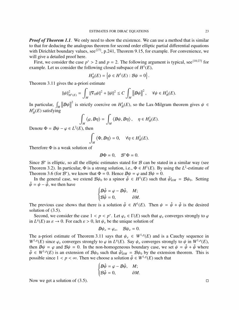
Proof of Theorem 1.1. We only need to show the existence. We can use a method that is similarto that for deducing the analogous theorem for second order elliptic partial differential equationswith Dirichlet boundary values, see [27], p.241, Theorem 9.15, for example. For convenience, wewill give a detailed proof here.

First, we consider the case p∗ > 2 and p = 2. The following argument is typical, see [10;27] forexample. Let us consider the following closed subspace of H1(E),

H1B(E) =

ψ ∈ H1(E) : Bψ = 0

.

Theorem 3.11 gives the a-priori estimate

∥ψ∥2H1(E) =

∫M∥∇0ψ∥2 + ∥ψ∥2 ≤ C

∫M

∥∥∥ /Dψ∥∥∥2, ∀ψ ∈ H1

B(E).

In particular,∫

M

∥∥∥ /Dψ∥∥∥2is strictly coercive on H1

B(E), so the Lax-Milgram theorem gives ψ ∈H1B(E) satisfying ∫

M

⟨φ, /Dη

⟩=

∫M

⟨/Dψ, /Dη

⟩, η ∈ H1

B(E).

Denote Φ = /Dψ − φ ∈ L2(E), then∫M

⟨Φ, /Dη

⟩= 0, ∀η ∈ H1

B(E).

Therefore Φ is a weak solution of

/DΦ = 0, B∗Φ = 0.

Since B∗ is elliptic, so all the elliptic estimates stated for B can be stated in a similar way (seeTheorem 3.2). In particular, Φ is a strong solution, i.e., Φ ∈ H1(E). By using the L2-estimate ofTheorem 3.6 (for B∗), we know that Φ = 0. Hence /Dψ = φ and Bψ = 0.

In the general case, we extend Bψ0 to a spinor ψ ∈ H1(E) such that ψ|∂M = Bψ0. Settingψ = ψ − ψ, we then have /Dψ = φ − /Dψ, M;

Bψ = 0, ∂M.

The previous case shows that there is a solution ψ ∈ H1(E). Then ψ = ψ + ψ is the desiredsolution of (3.5).

Second, we consider the case 1 < p < p∗. Let φε ∈ Γ(E) such that φε converges strongly to φin Lp(E) as ε→ 0. For each ε > 0, let ψε be the unique solution of

/Dψε = φε, Bψε = 0.

The a-priori estimate of Theorem 3.11 says that ψε ∈ W1,p(E) and is a Cauchy sequence inW1,p(E) since φε converges strongly to φ in Lp(E). Say ψε converges strongly to ψ in W1,p(E),then /Dψ = φ and Bψ = 0. In the non-homogeneous boundary case, we set ψ = ψ + ψ whereψ ∈ W1,p(E) is an extension of Bψ0 such that ψ|∂M = Bψ0 by the extension theorem. This ispossible since 1 < p < ∞. Then we choose a solution ψ ∈ W1,p(E) such that /Dψ = φ − /Dψ, M;

Bψ = 0, ∂M.

Now we get a solution of (3.5).


4. Dirac equations along a map

We first consider the following system which is slightly more general than (1.1):

(4.1)

/DψA + ΩAB · ψB = ηA, M;

BψA = BψA0 , ∂M,

A = 1, · · · , q, here ηA ∈ Lp(E),BψA0 ∈ W1−1/p,p(E|∂M) and Ω ∈ Ω1 (son), i.e., ΩA

B = −ΩBA. Under

suitable conditions, we can solve this system.

Theorem 4.1. Let M, E be as in Theorem 1.1. Suppose that Γ ∈ Dp∗(E), dΩ ∈ Lp∗(M),Ω ∈L2p∗(M). Then for 1 < p < p∗, (4.1) admits a unique solution. Moreover, we have the followingelliptic estimate

∥ψ∥W1,p(E) ≤ c(∥η∥Lp(E) + ∥Bψ0∥W1−1/p,p(E|∂M)

),

where c = c(p, ∥Γ∥p∗ , ∥Ω∥L2p∗ (M) + ∥dΩ∥Lp∗ (M)

)> 0.

Proof. We construct a new Dirac bundle and a new chirality operator, and then we can apply theexistence and uniqueness for the usual Dirac equation to prove this theorem.

Let E = ⊕nE = E ⊕ . . . ⊕ E︸︷︷︸n times

. Then E becomes a Dirac bundle as a Whitney sum bundle. The

Clifford multiplication is defined as

γ(X)(ψA) B (X · ψA),∀X ∈ T M,

i.e., γ = γE Id. Here γE(X)ψA B X · ψA stands for the Clifford multiplication on E. Then theassociated Γ = Γ Id, i.e.,

Γ(X)(ψA) B (Γ(X)ψA).Define Γ′ by

Γ′(X)(ψA) B (ΩAB(X)ψB).

It is clear that Γ′ ∈ Ω1(Ad(E)). We need only to check that [Γ′, γ] = 0 in order to prove thatΓ′ ∈ Dp∗(E). In fact,

[Γ′, γ](X,Y)(ψA) =(ΩA

B(X)(Y · ψB

)− Y ·ΩA

B(X)ψB)= 0.

Therefore, we have constructed a new Dirac bundle E with the Dirac operator D defined by

/D(ψA) = ( /DψA + ΩAB · ψB).

It is obvious that d(Γ + Γ′) ∈ Lp∗(M), Γ + Γ′ ∈ L2p∗(M).Introduce an operator G ∈ hom(E),

G(ψA) B (GψA).

It is clear thatG2 = Id, G∗ = G, Gγ(X) = −γ(X)G, ∀X ∈ T M.

Moreover, ∇G = 0. In fact,

∇XG(ψA) =(∇XGψA + ΩA

B(X)GψB)=

(G∇Xψ

A +GΩAB(X)ψB

)= G∇X(ψA).

In particular, G is a chirality operator on E. Therefore, the associated chirality boundary operator

B(ψA) B(BψA

).


Then we can use the theory of the Dirac equation Theorem 1.1 to finish the proof of this theorem.

Now we suppose that M is a Riemannian spin manifold with boundary ∂M and give the

Proof of Theorem 1.2. Embedding N into some Euclidian space, then as shown in section 2, wecan rewrite this boundary value problem for the Dirac equation as/∂ΨA + ΩA

B · ΨB = ηA, M;BΨA = BψA, ∂M,

whereΩA

B = [ν(Φ), dν(Φ)]AB.

In particular, dΩ = [dν(Φ), dν(Φ)]. Therefore, if Φ ∈ W1,2p∗(M,N), then Φ ∈ C0(M,N) by usingthe Sobolev embedding theorem. As a consequence,

Ω ∈ L2p∗(M), dΩ ∈ Lp∗(M).

Hence, by using the Theorem 4.1, we get a unique solution of Ψ ∈ W1,p(ΣM⊗Φ−1TRq) for somelarger q. Moreover, there exists a constant c = c

(p, ∥Φ∥W1,2p∗ (M)

)> 0 such that

∥Ψ∥W1,p(M) ≤ c(∥η∥Lp(M) + ∥Bψ∥W1−1/p,p(∂M)

).

Now we want to prove that Ψ is a spinor along the map Φ. Introduce ΨA = νABΨ

B, then weneed only to prove that Ψ = 0.

Claim. /∂ΨA + ΩAB · ΨB = 0, M;

BΨA = 0, ∂M.

If this claim is true, then using the Theorem 4.1 again, we get that Ψ = 0. Hence, we completethe proof of this theorem.

Now, we confirm the claim. In fact, noticing that νABη

B = 0, νABBψB = 0 since η is a spinor

along the map Φ and Bψ is the restriction of a spinor along the map Φ to the boundary ∂M, wehave that

/∂ΨA =νAB/∂ψ

B + dνAB · ΨB = −νA

BdνBC · ΨC + νA

BdνBCν

CD · ΨD + νA

BηB + dνA

B · ΨB

=dνAB · ΨB = −dπA

B · ΨB =(dπA

CπCB − πA

CdπCB

)· ΨB =

(dνA

CνCB − νA

CdνCB

)· ΨB

= −ΩAB · ΨB,

and

BΨA = νABBΨB = νA

BBψB = 0.

Remark 4.1. Using the same method, one can prove that /Dψ = η ∈ Lp(E ⊗ Φ−1V

), M;

BΨ = Bψ ∈ W1−1/p,p((

E ⊗ Φ−1V)|∂M

), ∂M


admits a unique solution Ψ ∈ W1,p(E ⊗Φ−1V), where E is a Dirac bundle on M, V is a Hermitianmetric vector bundle on N, /D is the associated Dirac operator of E ⊗Φ−1V , the Dirac connection∇ = ∇0 + Γ satisfies the condition Γ ∈ Dp∗E and Φ ∈ W1,2p∗(M; N).

Remark 4.2. IfΦ is smooth, then ΣM⊗Φ−1T N is a smooth Dirac bundle, in this case, Theorem 1.2is just a direct corollary of Theorem 1.1.

Now let us give some further remarks on the Schauder theory of Dirac equations. The interiorSchauder estimate for the Dirac equation is

Theorem 4.2 (See [1]). Let M, E be as in Theorem 1.1. Suppose that /Γ ∈ Cα(M) for some 0 <α < 1, then for all M′ ⋐ M′′ ⋐ M,

∥ψ∥1+α;M′ ≤ c(α, dist(M′, ∂M′′),

∥∥∥/Γ∥∥∥α;M′′

) (∥∥∥ /Dψ∥∥∥α;M′′+ ∥ψ∥0;M′′

).

Due to Proposition 3.1, one can also state a boundary Schauder estimate for the Dirac equation.

Theorem 4.3. Let M, E be as in Theorem 1.1. Suppose that /Γ ∈ Cα(M) for some 0 < α < 1, then

∥ψ∥1+α;M ≤ c(α,

∥∥∥/Γ∥∥∥α:M

) (∥∥∥ /Dψ∥∥∥α;M+ ∥Bψ∥1+α;∂M + ∥ψ∥0;M

).

Proof. The classical argument for Schauder estimates (see [27]) can be combined with Proposition 3.1.

By using the main Lp-estimates of Theorem 1.1, we can get

Theorem 4.4. Let M, E be as in Theorem 1.1. Suppose that Γ ∈ D1(E), Γ ∈ Cα(M) and dΓ ∈Cα(M) for some 0 < α < 1, then

∥ψ∥1+α;M ≤ c(α, ∥Γ∥α:M + ∥dΓ∥α;M

) (∥∥∥ /Dψ∥∥∥α;M+ ∥Bψ∥1+α;∂M

).

Proof. By using the main Lp-estimates of Theorem 1.1, we know that for large p

∥ψ∥0;M ≤c(p, ∥Γ∥p∗)(∥∥∥ /Dψ∥∥∥


)≤c

(α, ∥Γ∥α:M + ∥dΓ∥α;M

) (∥∥∥ /Dψ∥∥∥α;M+ ∥Bψ∥1+α;∂M

).

Then applying Theorem 4.3, we prove the desired result.

Similarly to the case of the Lp-estimate, we can prove the following two theorems:

Theorem 4.5. Let M, E be as in Theorem 1.1. Suppose that Γ ∈ D1(E),Γ ∈ Cα(M), dΓ ∈Cα(M),Ω ∈ Cα(M), dΩ ∈ Cα(M) for some 0 < α < 1. Let η ∈ Cα(M),Bψ0 ∈ C1,α(∂M), then(4.1) admits a unique solution ψ ∈ C1,α(M). Moreover, the following estimate holds

∥ψ∥1+α;M ≤ c(α, ∥Γ∥α;M + ∥dΓ∥α;M , ∥Ω∥α;M + ∥dΩ∥α;M

) (∥∥∥ /Dψ∥∥∥α;M+ ∥Bψ∥1+α;∂M

).

Theorem 4.6. Let M,N be as in Theorem 1.2. Let Φ ∈ C1,α(M,N) for some 0 < α < 1, then thefollowing Dirac equation /DΨ = η ∈ Cα(M;ΣM ⊗ Φ−1T N), M;

BΨ = Bψ ∈ C1,α(∂M;ΣM ⊗ Φ−1T N

), ∂M


admits a unique solution Ψ ∈ C1,α(M : ΣM ⊗ Φ−1T N), where /D is the Dirac operator along themap Φ. Moreover,

∥Ψ∥α;M ≤ c(α, ∥Φ∥1+α;M)(∥η∥α;M + ∥Bψ∥1+α;∂M

).

5. Short time existence of first order Dirac-harmonic map flows

In this section, we assume that Mm (m ≥ 2) is a compact Riemannian spin manifold withboundary ∂M and choose a fixed spin structure on M.

Let us consider the family of coupled system of differential equations for a map Φ : M ×[0,T ] −→ Rq with Φ = (ΦA) and for a spinor field Ψ : M × [0,T ] −→ ΣM ⊗ Φ−1TRq withΨ = (ΨA) along the map Φ

(∂

∂t− ∆

)ΦA + ΩA

B · dΦB +⟨ΩA

B, dΦB⟩= 0, M × (0, T ];

/∂ΨA + ΩAB · ΨB = 0, ∂M × [0, T ]

(5.1)

with the initial and boundary conditionsΦ(x, t) = ϕ(x, t), (x, t) ∈ ∂M × [0,T ] ∪ M × 0 ;BΨ = Bψ, ∂M × [0,T ],

(5.2)

where B is a chirality boundary operator.

Lemma 5.1. Suppose the image of Φ lies in N and Ψ is a spinor along the map Φ, then (Φ,Ψ)satisfies the Dirac-harmonic map flow (1.5), i.e.,∂tΦ = τ(Φ) − R(Φ,Ψ),

/DΨ = 0,

if and only if (Φ,Ψ) satisfies (5.1).

Proof. A well-known computation.

Lemma 5.2. Suppose that (Φ,Ψ) is a solution of (5.1) which is continuous on M × [0,T ] withϕ(x, t) ∈ N for all (x, t) ∈ ∂M × [0,T ]∪M × 0 and ψ is a spinor along the map ϕ|∂M for all time[0,T ]. Suppose Φ(x, t) ∈ N on M × (0,T ], then Φ(x, t) ∈ N for all (x, t) ∈ M × [0,T ] and Ψ(·, t)is a spinor along the map Φ(·, t) for all time t ∈ [0,T ]. In fact, ΨA = νA

BΨB satisfies the following

Dirac-type equation /∂ΨA + ΩAB · ΨB = 0, M;

BΨ = 0, ∂M.

Proof. For z ∈ Rq, let us define ρ : Rq −→ Rq by ρ(z) = z − π(z). Consider

φ(x, t) = ∥ρ(Φ(x, t))∥2 =q∑

A=1

∥∥∥ρA(Φ(x, t))∥∥∥2.


We can get that(∂

∂t− ∆

)φ(x, t) = −2 ∥∇ρ(Φ(x, t))∥2 + 2 ⟨∂tρ − ∆ρ, ρ⟩

= − 2 ∥∇ρ(Φ(x, t))∥2 + 2⟨νA

B

(∂tΦ

B − ∆ΦB)− πA

BC

⟨∇ΦB,∇ΦC

⟩, ρA

⟩= − 2 ∥∇ρ(Φ(x, t))∥2 − 2

⟨νA

B(Φ)(Ω(Φ)B

C · dΦC +⟨Ω(Φ)B

C, dΦC⟩)+ πA

BC(Φ)⟨∇ΦB,∇ΦC

⟩, ρ(Φ)A

⟩.

If Φ = π(Φ), then⟨νA

B(Φ)(Ω(Φ)B

C · dΦC +⟨Ω(Φ)B

C, dΦC⟩)+ πA

BC(Φ)⟨∇ΦB,∇ΦC

⟩, ρ(Φ)A

⟩= 0.

Therefore, we have the following estimate by applying the mean value theorem(∂

∂t− ∆

)φ ≤ Cφ.

Since φ ≥ 0 and φ = 0 on ∂M × [0,T ] ∪ M × 0, we have that φ = 0 on M × [0,T ]. HenceΦ(x, t) ∈ N for all (x, t) ∈ M × [0,T ] according to the maximum principle.

Next we show that Ψ is a spinor along the map Φ. In order to do this, we consider ΨA = νABΨ

B,then

/∂ΨA =νAB/∂Ψ

B + ∇νAB · ΨB = −νA

B∇νBC · ΨC + ∇νA

B · ΨB

=∇νAB · ΨB = −∇πA

B · ΨB

=(∇πA

CπCB − πA

C∇πCB

)· ΨB = −ΩA

B · ΨB.

Moreover, ΨA satisfies the following boundary conditions

BΨA = 0

for all time t ∈ [0,T ]. By the uniqueness of solutions of Dirac equations with chiral boundaryvalues, see Theorem 4.1, we get that Ψ = 0, i.e., Ψ is a spinor along the map Φ.

To state the short time existence for the Dirac-harmonic map flow, we first recall some basicfacts of heat kernels on Riemannian manifolds. An important property is that the heat kernel isalmost Euclidean [19;37]. In other words, if p is a heat kernel, then p and E are of the same order,locally uniformly in (x, y) as t → 0+, and a similar statement holds for the first derivatives of pand E, where

E(x, y, t) = (4πt)−m/2e− dist2(x,y)/(4t).

One can show that the Dirichlet heat kernel h(x, y, t) is also almost Euclidean [19], hence

h(x, y, t) ≤ ct−m/2e− dist2(x,y)/(4t),

and

∥∇h(x, y, t)∥ ≤ ct−m/2−1e− dist2(x,y)/(4t) dist(x, y).

We summarize these properties in


Lemma 5.3 (See [19;34]). For ever β > 0, there exists a constant c = c(β) such that

h(x, y, t) ≤ c(β)t−m/2+β dist(x, y)−2β,

∥∇h(x, y, t)∥ ≤ c(β)t−m/2−1+β dist(x, y)1−2β,

and

∥∇nh(x, y, t)∥ ≤ c(β)t−m/2−1+β dist(x, y)2−2β, x, y ∈ ∂M,

as t → 0+.

Proof. It is a consequence of the following inequality

xβe−x ≤ ββe−β, ∀x > 0, β > 0.

The improvement in the exponent of dist(x, y) in the third inequality is due to the fact that thederivative is in the direction normal to the boundary ∂M.

Now we can give a proof of the main Theorem 1.3.

Proof of Theorem 1.3. We will split the proof into four steps.

Step I Short time existence for the flow (5.1) and (5.2).

Let h(x, y, t) be the Dirichlet heat kernel of M. Define an operator T by

Tu(x, t) = u0(x, t) −∫ t

0

∫M

h(x, y, t − τ)(Ω(u) · du +

⟨Ω(u,Ψ(u)), du

⟩)(y, τ) dy dτ,

where

u0(x, t) =∫

Mh(x, y, t)ϕ(y, 0) dy −

∫ t

0

∫∂M

∂h∂ny

(x, y, t − τ)ϕ(y, τ) dσ(y) dτ.

Here

Ω(u) = [ν(u), dν(u)],

and

Ω(u,Ψ(u)) =12

RABCD(u)

(Ψ(u)C, ei · Ψ(u)D

)ηi C R(u)(Ψ(u),Ψ(u)),

where Ψ(u) is the unique solution of/∂ΨA = −Ω(u)AB · ΨB, M;

BΨA = BψA, ∂M

according to Theorem 4.1.It is clear that u0 is the unique solution of

∂

∂tu0 = ∆u0, M × (0,∞);

u0 = ϕ, ∂M × [0,∞) ∪ M × 0 .


For every ε > 0 and each u ∈ ∩0<t<εC1,0,0(M × [t, ε]) ∩C0(Mε), define the norm

∥u∥ B ∥u∥C0(M×[0,ε]) + supt∈[0,ε]∥∇u(·, t)∥C0(M) .

Let Xεϕ be the completion of the following subset of C0(Mε)

u ∈ ∩0<t<εC1,0,0(M × [t, ε]) ∩C0(Mε) : u = ϕ on PMε

.

HereMε B M × (0, ε], PMε B ∂M × [0, ε] ∪ M × 0 .

For u ∈ Xεϕ, according to Theorem 4.1 we have that for large p

∥Ψ(·, t)∥Cα(M) ≤c(p) ∥Ψ(·, t)∥W1,p(M) ≤ C(∥u∥) ∥BΨ0(·, t)∥W1−1/p,p(∂M)

≤C(∥u∥) ∥BΨ0(·, t)∥C1,α(∂M) ≤ C(∥u∥) ∥Bψ∥C1,0,α(∂Mε) .

As a consequence,T : Xε

ϕ −→ Xεϕ

is well defined. For δ > 0, let Bδ =u ∈ Xε

ϕ : ∥u − u0∥ ≤ δ.

According to Lemma 5.3, for every β > 0,

h(x, y, t) ≤ c(β)tβ−m/2 dist(x, y)−2β,

∥∇h(x, y, t)∥ ≤ c(β)tβ−1−m/2 dist(x, y)1−2β,

and

∥∇nh(x, y, t)∥ ≤ c(β)tβ−1−m/2 dist(x, y)2−2β, x, y ∈ ∂M.

1) u0 ∈ Xεϕ.

Let v0 = u0 − ϕ, then∂tv0 − ∆v0 = ∆ϕ − ∂tϕ C f , MT ;v0 = 0, PMT .

Since ϕ ∈ C2,1,α(MT ), we know that f ∈ C0,0,α(MT ) and

∥ f ∥C0(MT ) ≤ c ∥ϕ∥C2,1,0(MT ) , ∥ f ∥C0,0,α(MT ) ≤ c(α) ∥ϕ∥C2,1,α(MT ) .

Moreover, v0 can be given in the following formula, for (x, t) ∈ MT ,

v0(x, t) =∫ t

0

∫M

h(x, y, t − τ) f (y, τ) dy dτ.

The Schauder estimates imply that v0 ∈ ∩0<t<TC2,1,α(M × [t,T ]) ∩ C0(MT ). Thefollowing estimates follow by straightforward computations.

|v0(x, t)| ≤ ∥ϕ∥C2,1,0(Mε) ε,

|∇v0(x, t)| ≤ c(β) ∥ϕ∥C2,1,0(Mε) εβ−1,


for all (x, t) ∈ Mε and β ∈ (m/2, (m + 1)/2). In fact,

|v0(x, t)| ≤∫ t

0

∫M

h(x, y, t − τ) | f (y, τ)| dy dτ

≤ ∥ f ∥C0(Mt)

∫ t

0

∫M

h(x, y, t − τ) dy dτ ≤ ∥ f ∥C0(Mt) t,

and

|∇v0(x, t)| ≤∫ t

0

∫M|∇xh(x, y, t − τ)| | f (y, τ)| dy dτ

≤c(β) ∥ f ∥C0(Mt)

∫ t

0

∫M|t − τ|−2+β dist(x, y)1−2β dy dτ ≤ c(β) ∥ f ∥C0(Mt) tβ−m/2.

where β ∈ (m/2, (m + 1)/2). Therefore u0 ∈ Xεϕ, and for δ, ε both small we have that

u0 ⊂ N if ϕ ⊂ N.

2) For ε small, T (Bδ) ⊂ Bδ.

Since u ∈ Bδ, we have ∥u∥ ≤ C1.

∥Ω(u)∥C0(M×[0,ε]) = ∥[ν(u), dν(u)]∥C0(M×[0,ε]) ≤ c supt∈[0,ε]∥∇u(·, t)∥C0(M) ≤ c(C1),

and ∥∥∥Ω(u,Ψ(u))∥∥∥

C0(M×[0,ε])≤c sup

t∈[0,ε]∥Ψ(·, t)∥2C0(M)

≤c(C1) supt∈[0,ε]∥Bψ(·, t)∥2H1−1/p,p(∂M)

≤c(C1) ∥Bψ∥2C1,0,α(∂M×[0,ε]) ≤ c(C1)C2,

for p large enough, and the second inequality has used Theorem 4.1. Hence,

∥Ω(u)∥C0(Mε) +∥∥∥Ω(u,Ψ(u))

∥∥∥C0(Mε)

≤ c(C1,C2),∀u ∈ Bδ.

As a consequence,

∥Tu − u0∥ ≤ c(β)c(C1,C2) ∥du∥C0(Mε) εβ−m/2,

for β ∈ (m/2, (m + 1)/2).

3) ∥Tu − Tv∥ ≤ 12∥u − v∥ for u, v ∈ Bδ and ε small.

First, we have,

Tu(x, t) − Tv(x, t) = −∫ t

0

∫M

h(x, y, t − τ)(Ω(u) · du +

⟨Ω(u,Ψ(u)), du

⟩)(y, τ) dy dτ

+

∫ t

0

∫M

h(x, y, t − τ)(Ω(v) · dv +

⟨Ω(v,Ψ(v)), dv

⟩)(y, τ) dy dτ.


Moreover, notice thatΩ(u) −Ω(v) =[ν(u), dν(u)] − [ν(v), dν(v)]

=[ν(u) − ν(v), dν(u)] + [ν(v), dν(u) − dν(v)],

and

Ω(u,Ψ(u)) − Ω(v,Ψ(v))=R(u)(Ψ(u),Ψ(u)) − R(v)(Ψ(v),Ψ(v))= (R(u) − R(v)) (Ψ(u),Ψ(u)) + R(v)(Ψ(u) − Ψ(v),Ψ(u)) + R(v)(Ψ(v),Ψ(u) − Ψ(v)),

we have

∥Ω(u) −Ω(v)∥C0(Mε) ≤ c(C1,C2) ∥u − v∥ ,

and∥∥∥Ω(u,Ψ(u)) − Ω(v,Ψ(v))∥∥∥

C0(Mε)≤c(C1,C2)

(∥u − v∥ + ∥Ψ(u) − Ψ(v)∥C0(M×[0,ε])

)≤c(C1,C2) ∥u − v∥ .

The last inequality follows from the following fact/∂(Ψ(u)A − Ψ(v)A

)= −Ω(u)A

B · (Ψ(u)B − Ψ(v)B) +(Ω(u)A

B −Ω(v)AB

)· Ψ(v)B, M;

B(Ψ(u) − Ψ(v)) = 0, ∂M.

And Theorem 4.1 implies that for large p∥Ψ(u) − Ψ(v)∥Cα(M) ≤c(p) ∥Ψ(u) − Ψ(v)∥W1,p(M) ≤ c(p,C1,C2) ∥u − v∥ ∥Ψ(v)∥Lp(E)

≤c(p,C1,C2) ∥u − v∥ .Thus,∥∥∥∥Ω(u) · du +

⟨Ω(u,Ψ(u)), du

⟩−Ω(v) · dv −

⟨Ω(v,Ψ(v)), dv

⟩∥∥∥∥Cα(M)

≤ c(p,C1,C2) ∥u − v∥ .

Using a similar argument for v0, one gets that

∥Tu − Tv∥ ≤ c(β)c(C1,C2)εβ−m/2 ∥u − v∥ ,where β ∈ (m/2, (m + 1)/2).

Therefore, there exists a fixed point of T in Bδ, i.e., we have proved the short timeexistence of (5.1) and (5.2).

Step II Regularity.

Let (Φ,Ψ) be the solution of (5.1) and (5.2) constructed above. The Theorem 4.1implies that Ψ ∈ L∞(Mε) and hence Φ ∈ ∩0<t<εC1,0,α(M × [t, ε]) ∩ C(Mε) by using theLp-estimate for the heat equation. For every 0 < t, τ ≤ ε, we have /∂

(ΨA(·, t) − ΨA(·, τ)

)= −ΩA

B(·, t) ·(ΨB(·, t) − ΨB(·, τ)

)+

(ΩA

B(·, τ) −ΩAB(·, t)

)· ΨB(·, τ), M;

B (Ψ(·, t) − Ψ(·, τ)) = B (ψ(·, t) − ψ(·, τ)) , ∂M.

Again by using Theorem 4.1, for larger p

∥Ψ(·, t) − Ψ(·, τ)∥Cα(M) ≤ c(p,C1,C2) |t − τ|α/2 .


Thus,Ψ ∈ ∩0<t<εC0,0,α(M×[t, ε])∩C0(Mε). The Schauder estimate for the heat equationimplies thatΦ ∈ ∩0<t<εC2,1,α(M×[t, ε])∩C0(Mε). The interior Schauder estimate for theDirac equation implies that Ψ(·, t) ∈ C2,α(M) for every t ≤ ε. If one uses the boundarySchauder estimate, one can get that Ψ(·, t) ∈ C1,α(M) for t ≤ ε.

Suppose thatlim supt<T1,t→T1

∥dΦ(·, t)∥C0(M) < ∞,

the discussion above implies that this flow can be extended to a larger time T ′1 > T1,hence T1 is not the maximum time which is a contradiction.

Step III Uniqueness.

Finally, we state the uniqueness. Suppose that (Φi,Ψi) are solutions of (5.1) and(5.2). Let u = Φ1 − Φ2, η = Ψ1 − Ψ2, then

|∂tu − ∆u| ≤ C |∇u| +C |u| +C |η| ,

and ∣∣∣/∂η + Ω1 · η∣∣∣ ≤ C |∇u| +C |u| .

Hence, applying Theorem 4.1 and using the same computation as for v0, we get that

∥η(·, t)∥C0(M) ≤ C ∥u∥ ,

and

∥u∥ ≤ C ∥u∥ εβ−m/2

holds for 0 < ε ≤ T1 and β ∈ (m/2, (m + 1)/2), where ∥·∥ is the norm corresponding toMε. Thus, if ε is small, then ∥u∥ = 0, i.e., u = 0 and hence η = 0. Then we can provethe uniqueness of the Dirac-harmonic heat flow by iteration.

Step IV Completion of the proof.

We have actually proved that Φ ⊂ N if ϕ ⊂ N. Therefore, we can use Lemma 5.2.As a consequence, Φ(·, t) ∈ N and Ψ(·, t) ∈ ΣM × Φ(·, t)−1T N for all 0 ≤ t < T1

since Bψ(·, t) ∈(ΣM ⊗ ϕ(·, t)−1T N

)|∂M for all t. Then applying Lemma 5.1, we finally

complete the proof of this theorem.

6. Dirac equations along a map between Riemannian disks

In this section, we discuss a Dirac equation along a smooth map ϕ : M = (D, λ |dz|2) −→ N =(D, ρ |dw|2) where D = |z| < 1 is the open unit disk on C. Let ΣM be the spin bundle on M.


Consider a Dirac bundle ΣM ⊗ ϕ−1T N and split this Dirac bundle as (see [36;44])

ΣM ⊗ ϕ−1T N

=(Σ+M ⊗ ϕ−1T 1,0N

)⊕

(Σ−M ⊗ ϕ−1T 1,0N

)⊕

(Σ+M ⊗ ϕ−1T 0,1N

)⊕

(Σ−M ⊗ ϕ−1T 0,1N

),

whereΣ+M = ψ ∈ ΣM : ∂z · ψ = 0 , Σ−M = ψ ∈ ΣM : ∂z · ψ = 0 .

We identify the Clifford multiplication by the orthogonal bases ∂z, ∂z with the following ma-trices (see [23;36]):

∂z = λ1/2

(0 01 0

), ∂z = λ

1/2(0 −10 0

).

And the spinor ψ ∈ ΣM ⊗ ϕ−1T N can be written as

ψ =

(f +

f −

)⊗ ∂ϕ +

(f +

f −

)⊗ ∂ϕ

with (10

)∈ Σ+M,

(01

)∈ Σ−M.

The connection on the spin bundle ΣM is then given by the following operators (see [36])

∇ΣM∂z=∂

∂z+

14∂ log λ∂z

, ∇ΣM∂z=∂

∂z+

14∂ log λ∂z

.

Therefore, the Dirac operator on ΣM ⊗ ϕ−1T N is of the following form

/D =2λ−1/2

0 − ∂

∂z− 1

4∂ log λ∂z

− ∂ log ρ∂ϕ

∂ϕ

∂z∂

∂z+

14∂ log λ∂z

+∂ log ρ∂ϕ

∂ϕ

∂z0

⊕ 2λ−1/2

0 − ∂

∂z− 1

4∂ log λ∂z

− ∂ log ρ∂ϕ

∂ϕ

∂z∂

∂z+

14∂ log λ∂z

+∂ log ρ∂ϕ

∂ϕ

∂z0

.The chiral boundary operator [22;23;29] is given by

B± = 12

(1 ±z−1

±z 1

)⊕ 1

2

(1 ±z−1

±z 1

).

Now we consider the following Dirac equation /Dψ = 0, D;B±ψ = B±ψ0, ∂D.

As discussed above, /Dψ = 0 is equivalent to the following systems

f +z +(14

(log λ)z + (log ρ)ϕϕz

)f + = 0, f −z +

(14


)f − = 0,


and

f +z +(14


)f + = 0, f −z +

(14


)f − = 0,

where the spinor ψ has the form

ψ =

(f +

f −

)⊗ ∂ϕ +

(f +

f −

)⊗ ∂ϕ.

Let g be a solution of the Riemannian-Hilbert problemgz =14

(log λ)z + (log ρ)ϕϕz, D;

Re g = log(λ1/4ρ1/2

), ∂D.

All solutions can be given in the following formulae [see [11], p.71, Theorem 21.]

g(z) =i Im g(0) + log λ1/4(z) +1

2πi

∫∂D

log(ρ(ϕ(ζ))1/2

)ζ

ζ + zζ − z

dζ

+1

4πi

∫D

((log ρ)ϕϕζ(ζ)

ζ

ζ + zζ − z

+(log ρ)ϕϕζ(ζ)

ζ

1 + zζ1 − zζ

)dζ ∧ dζ,

for all z ∈ D. Then

f +z + gz f + = 0, f − z +((log ρ + log λ1/2)z − gz

)f − = 0,

and

f +z +((log ρ + log λ1/2)z − gz

)f + = 0, f − z + gz f − = 0.

Therefore, there exist four holomorphic functions A+, A−, A+, A− such that

f + = e−gA+, f − = λ−1/2ρ−1egA−, f + = λ−1/2ρ−1egA+, f − = e−gA−.

The chirality boundary condition B±ψ = B±ψ0 now is equivalent to

A+ ± z−1A− = λ1/4ρ1/2ei Im g(

f +0 ± z−1 f −0), A+ ± z−1A− = λ1/4ρ1/2e−i Im g

(f +0 ± z−1 f −0

),

for z ∈ ∂D, where

ψ0 =

(f +0f −0

)⊗ ∂ϕ +

(f +0f −0

)⊗ ∂ϕ.

Since the index of z−1 is−1, the solutions A+, A−, A+, A− must be unique according to Theorem A.1(see Appendix A). In particular, f +, f −, f +, f − are independent of the choice of g. In fact, wecan write any other choice of g by g + ic where c is some real number. Then the solutionsA+, A−, A+, A− must be replaced by eicA+, e−icA−, e−icA+, eicA− respectively. As a consequence,f +, f −, f +, f − do not change.

Next, we construct these solutions by using Theorem A.1. Denote

F(z) B1

2πi

∫∂D

λ1/4(ζ)ρ(ϕ(ζ))1/2ei Im g(ζ)( f +0 (ζ) ± ζ−1 f −0 (ζ))ζ − z

dζ, z < ∂D


and

F(z) B1

2πi

∫∂D

λ1/4(ζ)ρ(ϕ(ζ))1/2e−i Im g(ζ)( f +0 (ζ) ± ζ−1 f −0 (ζ))ζ − z

dζ, z < ∂D.

Then

A+(z) = F(z), A−(z) = ±z−1F(1/z), A+(z) = F(z), A−(z) = ±z−1F(1/z), z ∈ D

are the solutions.To summarize the previous discussion and using Theorem A.2 (see Appendix A), we have the

following

Theorem 6.1. Suppose that ϕ ∈ C1+α(D) and B±ψ0 ∈ C1+α(∂D) for some α ∈ (0, 1), then thereexits a unique solution ψ ∈ C1+α(D) of /Dψ = 0, D;

B±ψ = B±ψ0, ∂D.

Moreover, there exists a constant c = c(α) such that

∥ψ∥1+α;D ≤ c∥∥∥B±ψ0

∥∥∥1+α;∂D

∥ϕ∥1+α;D .

Remark 6.1. When the domain is D = |z| < 1, the MIT bag boundary operator is given by

B±MIT =12

(1 ∓iz−1

±iz 1

)⊕ 1

2

(1 ∓iz−1

±iz 1

).

The index of ∓iz−1 is −1 and therefore we can use the Theorem A.1 and Theorem A.2 (seeAppendix A). In particular, the above theorem is also true for MIT bag boundary value con-ditions.

Appendix A. The boundary value problem for the ∂-equation

Let D = z ∈ C : |z| < 1 be the open unit disk in the complex plain C. We say that (A+, A−) isa holomorphic function pair on D if A+, A− are two holomorphic functions on D. Consider thefollowing transformation

A+(z) B A+(z), ∀z ∈ D+ B D,

and

A−(z) B A−(1/z), ∀z ∈ D− B C \ D.

Then A+ and A− are holomorphic in D+ and D− respectively. Moreover, if A+, A− satisfy thefollowing boundary condition

A+ − φA− = f , on ∂D,

then A+, A− satisfy the following boundary condition

A+ − φA− = f , on ∂D.


Theorem A.1 (See [11], p.39, Theorem 14., p.42, Theorem 15., p.11, Theorem 5.). Suppose thatφ ∈ Cα(∂D) with φ(ζ) , 0 for all ζ ∈ ∂D, where 0 < α < 1. Let f ∈ Cα(∂D) and κ be the indexof φ. Then if κ ≥ 0, there exist exactly κ + 1 linearly independent holomorphic function pairs(A+, A−) on D such that

A+ − φA− = 0

is satisfied on the boundary ∂D. If κ = −1, then there exists a unique holomorphic function pair(A+, A−) such that

A+ − φA− = f

holds on the boundary. Moreover, A± ∈ Cα(D) ∩ A(D). In fact, if we set

γ(z) B1

2πi

∫∂D

log (ζφ(ζ))ζ − z

dζ, z < ∂D,

and

ψ(z) B1

2πi

∫∂D

f (ζ)e−γ(ζ)

ζ − zdζ, z < ∂D,

then the holomorphic pair (A+, A−) is

A+(z) = eγ(z)ψ(z), A−(z) = z−1eγ(1/z)ψ(1/z), z ∈ D.

Moreover, there exists a constant c = c(α) such that∥∥∥A±∥∥∥α;D≤ c ∥φ∥α;D ∥ f ∥α;D .

We also need the following Schauder estimate.

Theorem A.2 (See [11], p.11, Theorem 5., p.84, Theorem 29.). Suppose that f ∈ Cα(D) andh ∈ C1+α(∂D) for some 0 < α < 1, then every solution ofsgz = f , D;

Re g = h, ∂D

is of class C1+α(D). Moreover, there exists a constant c = c(α) such that

∥g∥1+α;D ≤ c(∥ f ∥α;D + ∥h∥1+α;∂D + |Im g(0)|

).

References

[1] B. Ammann, A variational problem in conformal spin geometry, Habilitationsschift, Uni-versitat Hamburg (2003). 26

[2] B. Ammann and N. Ginoux, Examples of Dirac-harmonic maps after Jost-Mo-Zhu, 2011.4

[3] , Dirac-harmonic maps from index theory, Calc. Var. Partial Differential Equations47 (2013), no. 3-4, 739–762. MR 3070562 4

[4] M. F. Atiyah, V. K. Patodi, and I. M. Singer, Spectral asymmetry and Riemannian geometry.I, Math. Proc. Cambridge Philos. Soc. 77 (1975), 43–69. MR 0397797 (53 #1655a) 1


[5] , Spectral asymmetry and riemannian geometry. ii, Mathematical Proceedings ofthe Cambridge Philosophical Society, vol. 78, Cambridge Univ Press, 1975, pp. 405–432.1

[6] , Spectral asymmetry and riemannian geometry. iii, Mathematical Proceedings ofthe Cambridge Philosophical Society, vol. 79, Cambridge Univ Press, 1976, pp. 71–99. 1

[7] W. Ballmann, J. Bruning, and G. Carron, Regularity and index theory for Dirac-Schrodingersystems with Lipschitz coefficients, J. Math. Pures Appl. (9) 89 (2008), no. 5, 429–476.MR 2416671 (2009c:58035) 2

[8] C. Bar, On nodal sets for Dirac and Laplace operators, Comm. Math. Phys. 188 (1997),no. 3, 709–721. MR 1473317 (98g:58179) 20

[9] C. Bar and W. Ballmann, Boundary value problems for elliptic differential operators of firstorder, Surveys in differential geometry. Vol. XVII, Surv. Differ. Geom., vol. 17, Int. Press,Boston, MA, 2012, pp. 1–78. MR 3076058 2, 8, 14

[10] R. A. Bartnik and P. T. Chrusciel, Boundary value problems for Dirac-type equations, J.Reine Angew. Math. 579 (2005), 13–73. MR 2124018 (2005k:58040) 2, 3, 14, 22, 23

[11] H. G. W. Begehr, Complex analytic methods for partial differential equations, World Sci-entific Publishing Co., Inc., River Edge, NJ, 1994, An introductory text. MR 1314196(95m:35031) 35, 37

[12] J.-M. Bismut and J. Cheeger, Families index for manifolds with boundary, superconnec-tions, and cones. I. Families of manifolds with boundary and Dirac operators, J. Funct.Anal. 89 (1990), no. 2, 313–363. MR 1042214 (91e:58180) 2

[13] B. Booss-Bavnbek, M. Marcolli, and B. L. Wang, Weak UCP and perturbed monopoleequations, Internat. J. Math. 13 (2002), no. 9, 987–1008. MR 1936783 (2003i:58064) 3, 20

[14] B. Booss-Bavnbek and K. P. Wojciechowski, Elliptic boundary problems for Dirac oper-ators, Mathematics: Theory & Applications, Birkhauser Boston, Inc., Boston, MA, 1993.MR 1233386 (94h:58168) 2, 3, 20

[15] V. Branding, On the evolution of regularized Dirac-harmonic maps from closed surfaces,arXiv preprint arXiv:1406.6274 (2014). 5

[16] J. Bruning and M. Lesch, Spectral theory of boundary value problems for Dirac type op-erators, Geometric aspects of partial differential equations (Roskilde, 1998), Contemp.Math., vol. 242, Amer. Math. Soc., Providence, RI, 1999, pp. 203–215. MR 1714487(2000i:58042) 2

[17] , On boundary value problems for Dirac type operators. I. Regularity and self-adjointness, J. Funct. Anal. 185 (2001), no. 1, 1–62. MR 1853751 (2002g:58034) 2

[18] T. Carleman, Sur un probleme d’unicite pur les systemes d’equations aux derivees partiellesa deux variables independantes, Ark. Mat., Astr. Fys. 26 (1939), no. 17, 9. MR 0000334(1,55f) 3, 20

[19] I. Chavel, Eigenvalues in Riemannian geometry, Pure and Applied Mathematics, vol. 115,Academic Press, Inc., Orlando, FL, 1984, Including a chapter by Burton Randol, With anappendix by Jozef Dodziuk. MR 768584 (86g:58140) 28, 29

[20] Q. Chen, J. Jost, J. Y. Li, and G. F. Wang, Regularity theorems and energy identities forDirac-harmonic maps, Math. Z. 251 (2005), no. 1, 61–84. MR 2176464 (2007a:58013) 4,10


[21] , Dirac-harmonic maps, Math. Z. 254 (2006), no. 2, 409–432. MR 2262709(2007k:58021) 4, 10

[22] Q. Chen, J. Jost, and G. F. Wang, The maximum principle and the Dirichlet problem forDirac-harmonic maps, Calc. Var. Partial Differential Equations 47 (2013), no. 1-2, 87–116.MR 3044133 4, 8, 34

[23] Q. Chen, J. Jost, G. F. Wang, and M. M. Zhu, The boundary value problem for Dirac-harmonic maps, J. Eur. Math. Soc. (JEMS) 15 (2013), no. 3, 997–1031. MR 3085099 4,11, 34

[24] P. Deligne, P. Etingof, D. S. Freed, L. C. Jeffrey, D. Kazhdan, J. W. Morgan, D. R. Morrison,and E. Witten (eds.), Quantum fields and strings: a course for mathematicians. Vol. 1,2, American Mathematical Society, Providence, RI; Institute for Advanced Study (IAS),Princeton, NJ, 1999, Material from the Special Year on Quantum Field Theory held at theInstitute for Advanced Study, Princeton, NJ, 1996–1997. MR 1701618 (2000e:81010) 4

[25] P.A. Dirac, The Quantum Theory of the Electron, Proceedings of the Royal Society of Lon-don. Series A, Containing Papers of a Mathematical and Physical Character, Vol. 117, No.778 (Feb. 1, 1928), pp. 610-624 1

[26] G. W. Gibbons, S. W. Hawking, G. T. Horowitz, and M. J. Perry, Positive mass theoremsfor black holes, Comm. Math. Phys. 88 (1983), no. 3, 295–308. MR 701918 (84k:83015) 2

[27] D. Gilbarg and N. S. Trudinger, Elliptic partial differential equations of second order,Classics in Mathematics, Springer-Verlag, Berlin, 2001, Reprint of the 1998 edition.MR 1814364 (2001k:35004) 23, 26

[28] M. Herzlich, A Penrose-like inequality for the mass of Riemannian asymptotically flat man-ifolds, Comm. Math. Phys. 188 (1997), no. 1, 121–133. MR 1471334 (99a:53039) 2

[29] O. Hijazi, S. Montiel, and A. Roldan, Eigenvalue boundary problems for the Dirac oper-ator, Comm. Math. Phys. 231 (2002), no. 3, 375–390. MR 1946443 (2004b:58034) 2, 8,34

[30] L. Hormander, L2 estimates and existence theorems for the ∂ operator, Acta Math. 113(1965), 89–152. MR 0179443 (31 #3691) 3, 15

[31] D. Jerison, Carleman inequalities for the Dirac and Laplace operators and unique contin-uation, Adv. in Math. 62 (1986), no. 2, 118–134. MR 865834 (88b:35218) 2, 3, 20

[32] J. Jost, Geometry and physics, Springer-Verlag, Berlin, 2009. MR 2546999 (2010k:58002)4

[33] , Riemannian geometry and geometric analysis, sixth ed., Universitext, Springer,Heidelberg, 2011. MR 2829653 15

[34] , Partial differential equations, third ed., Graduate Texts in Mathematics, vol. 214,Springer, New York, 2013. MR 3012036 29

[35] J. Jost, X. H. Mo, and M. M. Zhu, Some explicit constructions of Dirac-harmonic maps, J.Geom. Phys. 59 (2009), no. 11, 1512–1527. MR 2569270 (2011a:53121) 4

[36] H. B. Lawson and M.-L. Michelsohn, Spin geometry, Princeton Mathematical Series,vol. 38, Princeton University Press, Princeton, NJ, 1989. MR 1031992 (91g:53001) 6,10, 18, 34

[37] P. Li, Geometric analysis, Cambridge Studies in Advanced Mathematics, vol. 134, Cam-bridge University Press, Cambridge, 2012. MR 2962229 28


[38] T. H. Parker and C. H. Taubes, On Witten’s proof of the positive energy theorem, Comm.Math. Phys. 84 (1982), no. 2, 223–238. MR 661134 (83m:83020) 2

[39] G. Schwarz, Hodge decomposition—a method for solving boundary value problems, Lec-ture Notes in Mathematics, vol. 1607, Springer-Verlag, Berlin, 1995. MR 1367287(96k:58222) 8

[40] B. Sharp and M. M. Zhu, Regularity at the free boundary for Dirac-harmonic maps fromsurfaces, arXiv preprint arXiv:1306.4260 (2013). 4, 8

[41] M. C. Shaw, L2-estimates and existence theorems for the tangential Cauchy-Riemann com-plex, Invent. Math. 82 (1985), no. 1, 133–150. MR 808113 (87a:35136) 15

[42] C. Y. Wang and D. L. Xu, Regularity of Dirac-harmonic maps, Int. Math. Res. Not. IMRN(2009), no. 20, 3759–3792. MR 2544729 (2010i:53120) 4

[43] E. Witten, A new proof of the positive energy theorem, Comm. Math. Phys. 80 (1981), no. 3,381–402. MR 626707 (83e:83035) 2

[44] L. Yang, A structure theorem of Dirac-harmonic maps between spheres, Calc. Var. PartialDifferential Equations 35 (2009), no. 4, 409–420. MR 2496649 (2010c:53095) 34

[45] M. M. Zhu, Regularity for weakly Dirac-harmonic maps to hypersurfaces, Ann. GlobalAnal. Geom. 35 (2009), no. 4, 405–412. MR 2506243 (2010b:53076) 4

School ofMathematics and Statistics, WuHan University, 430072 Hubei, ChinaE-mail address: [email protected]

Max Planck Institute forMathematics in the Sciences, Inselstrasse 22, 04103 Leipzig, GermanyE-mail address: [email protected]

School ofMathematics and Statistics, WuHan University, 430072 Hubei, China



Date post:	27-Aug-2018
Category:	Documents
Upload:	phungtuong
View:	219 times
Download:	0 times

Max-Planck-Institut fur Mathematik¨ in den ... · these estimates to a new nonlinear...

Documents