20-WMWDPre-6-07.ppt

Maximizing Secondary Clarifier Capacity with Three- dimensional Modeling

Randal Samstag and Ed WickleinCarollo Engineers

20-WMWDPre-6-07.ppt

Presentation Outline

• Introduction to the problem• Comparison of models• Case studies:

Center feed circular radial flowCenter feed square radial flowPeripheral feed square countercurrent flowRectangular lamella clarifiers

20-WMWDPre-6-07.ppt

The Clarifier

• Used for both primary and secondary separation of solids

• Efficiency depends on Settling characteristicsTank geometry

• The good news:Both settleability and tank geometry can often be improved

20-WMWDPre-6-07.ppt

Settleability Can be Improved

• Analysis of the biological populations is crucial

• Selectors encourage populations that settle well

• Depends on:ConfigurationSRT

20-WMWDPre-6-07.ppt

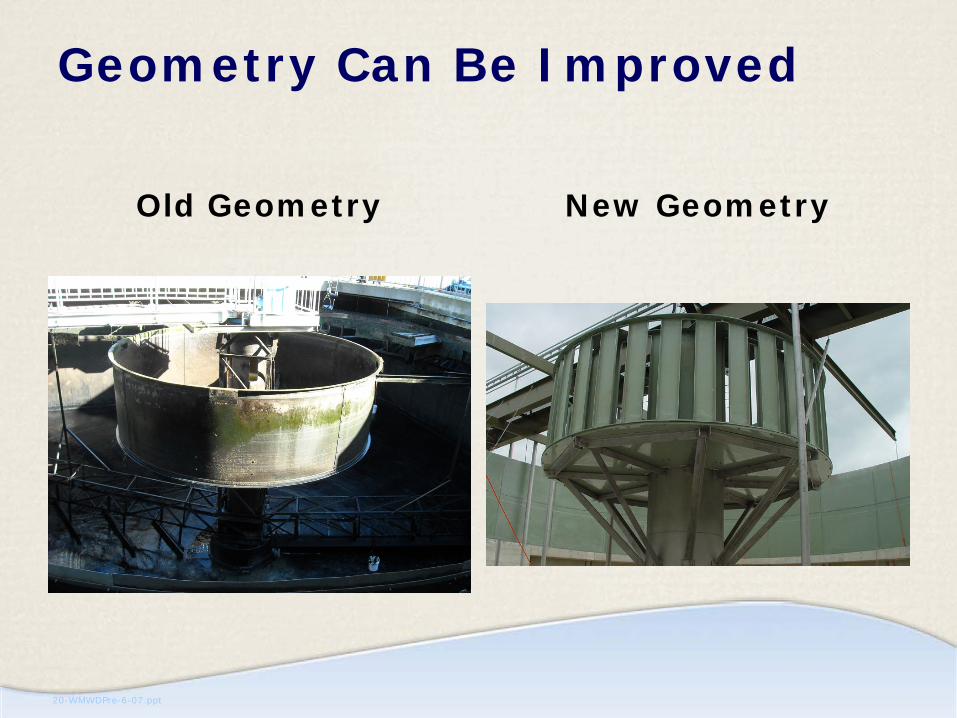
Geometry Can Be Improved

Old Geometry New Geometry

20-WMWDPre-6-07.ppt

Why do Modeling?

• Thirty years of development using computational fluid dynamics (CFD) for analysis of sedimentation has proven that CFD can 1) Capture the main features of clarifier

behavior2) Model detailed features of hydraulic behavior3) Efficiently predict performance of novel

designs4) Be more cost effective than full-scale

prototypes

20-WMWDPre-6-07.ppt

Types of Sedimentation Models

• Solids flux models (state point analysis)• One-dimensional dynamic models

(Biowin, Sedtank, Takacs, Vitasovic, Stenstrom)

• Two-dimensional dynamic models (UNO, TANKXZ, Carollo Fluent UDF)

• Three-dimensional dynamic models (Zhou/McCorquodale, Carollo Fluent UDF)

20-WMWDPre-6-07.ppt

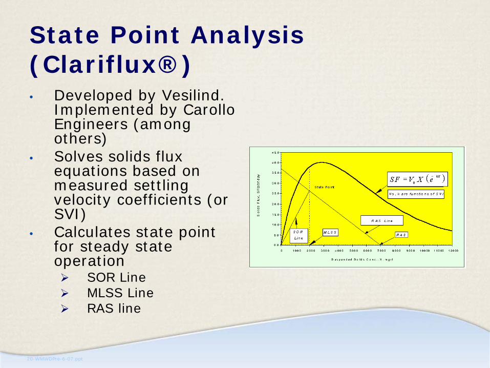
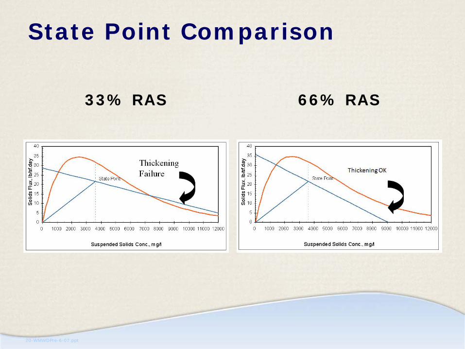
State Point Analysis (Clariflux®)• Developed by Vesilind.

Implemented by Carollo Engineers (among others)

• Solves solids flux equations based on measured settling velocity coefficients (or SVI)

• Calculates state point for steady state operation

SOR LineMLSS LineRAS line

20-WMWDPre-6-07.ppt

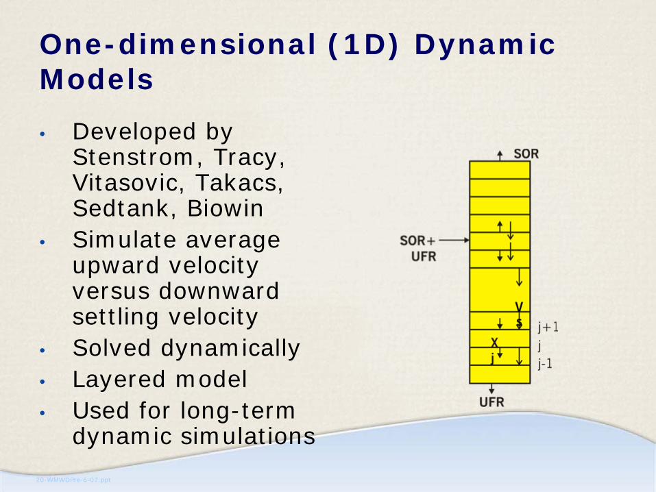
One-dimensional (1D) Dynamic Models

• Developed by Stenstrom, Tracy, Vitasovic, Takacs, Sedtank, Biowin

• Simulate average upward velocity versus downward settling velocity

• Solved dynamically• Layered model• Used for long-term

dynamic simulations

20-WMWDPre-6-07.ppt

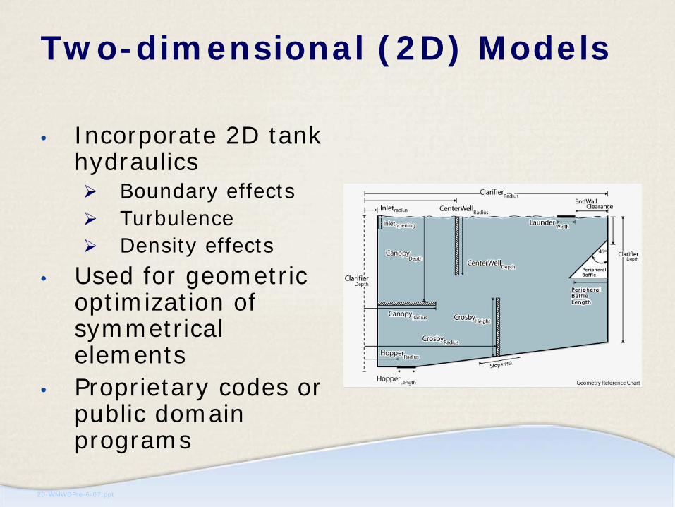
Two-dimensional (2D) Models

• Incorporate 2D tank hydraulics

Boundary effectsTurbulenceDensity effects

• Used for geometric optimization of symmetrical elements

• Proprietary codes or public domain programs

20-WMWDPre-6-07.ppt

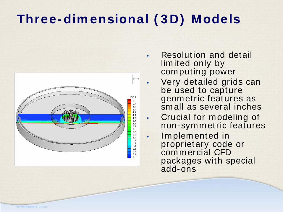
Three-dimensional (3D) Models

• Resolution and detail limited only by computing power

• Very detailed grids can be used to capture geometric features as small as several inches

• Crucial for modeling of non-symmetric features

• Implemented in proprietary code or commercial CFD packages with special add-ons

20-WMWDPre-6-07.ppt

Each Type of Model Has its Place• State Point Analysis – Steady State

Capacity Analysis• 1D Dynamic Models – Long-term

Dynamic simulations• 2D Models – Simple design evaluations• 3D Models – For design problems that are

not simple

20-WMWDPre-6-07.ppt

Examples of 3D Problems

• Analysis of inlet conditionsAlmost all inlet flow is three-dimensional

• Analysis of tank shapes that are not simple

Square radial flow tanksCircular peripheral feed tanksCircular or square peripheral feed and withdrawal tanksTanks with eccentric baffles or effluent troughs

20-WMWDPre-6-07.ppt

Case Studies

• Center feed square radial flow• Center feed circular radial flow• Square peripheral feed / withdrawal• Rectangular lamella clarifiers

20-WMWDPre-6-07.ppt

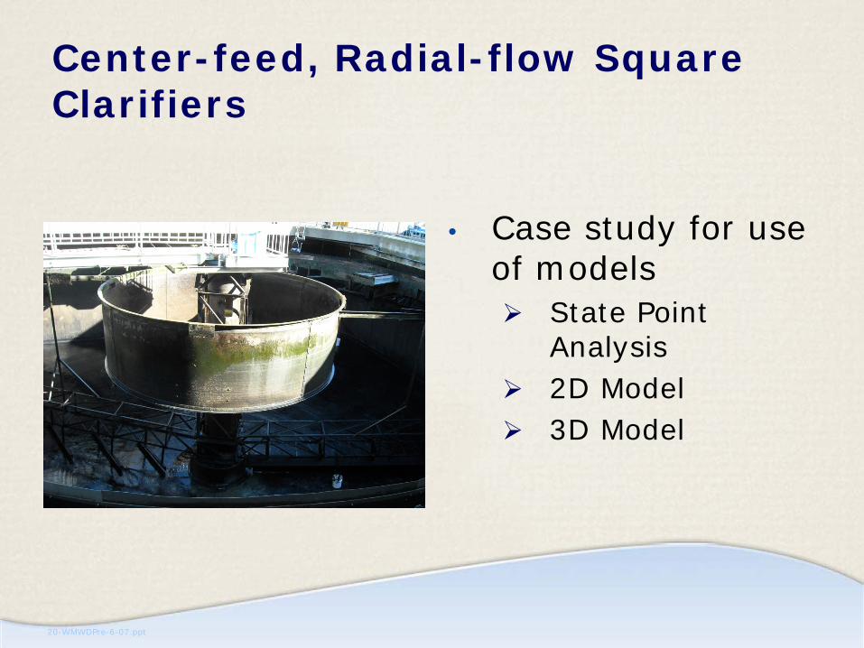
Center-feed, Radial-flow Square Clarifiers

• Case study for use of models

State Point Analysis2D Model3D Model

20-WMWDPre-6-07.ppt

State Point Comparison

33% RAS 66% RAS

20-WMWDPre-6-07.ppt

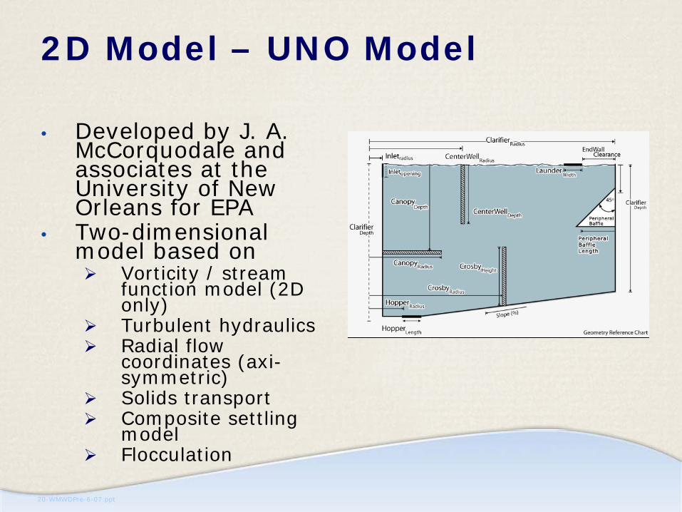
2D Model – UNO Model

• Developed by J. A. McCorquodale and associates at the University of New Orleans for EPA

• Two-dimensional model based on

Vorticity / stream function model (2D only)Turbulent hydraulicsRadial flow coordinates (axi-symmetric)Solids transportComposite settling modelFlocculation

20-WMWDPre-6-07.ppt

2D Model Results Test Calibration Results

FieldUNO Model

20-WMWDPre-6-07.ppt

2D Model Results Summary of Model Runs

20-WMWDPre-6-07.ppt

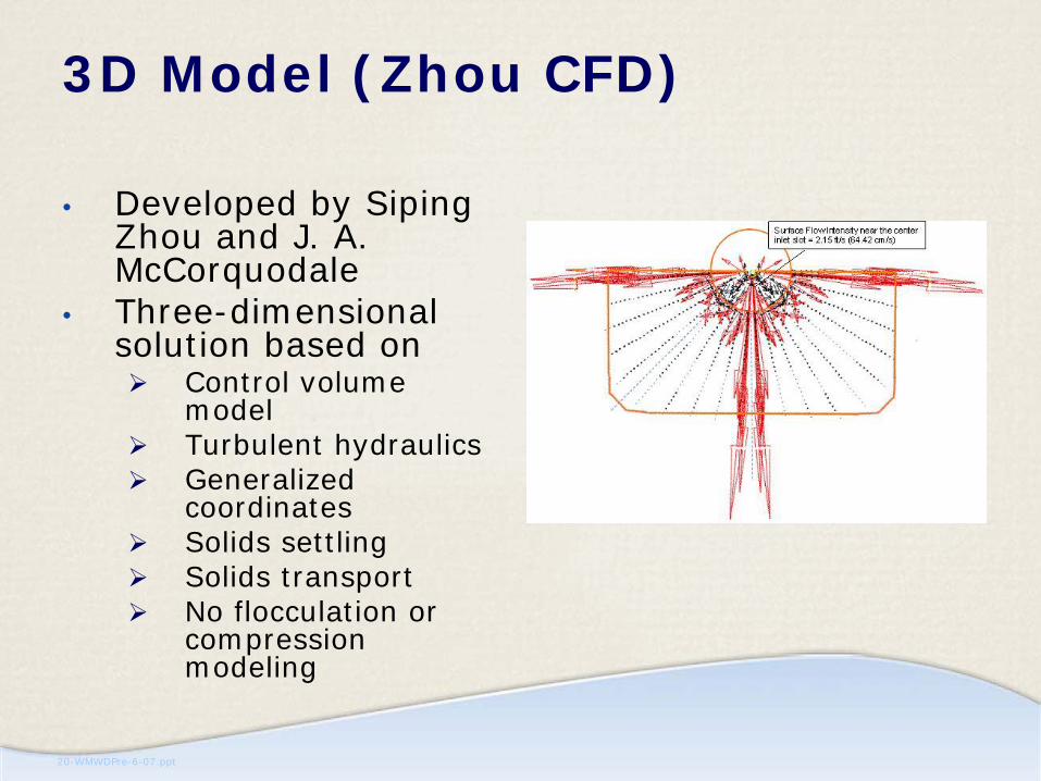
3D Model (Zhou CFD)

• Developed by Siping Zhou and J. A. McCorquodale

• Three-dimensional solution based on

Control volume modelTurbulent hydraulicsGeneralized coordinatesSolids settlingSolids transportNo flocculation or compression modeling

20-WMWDPre-6-07.ppt

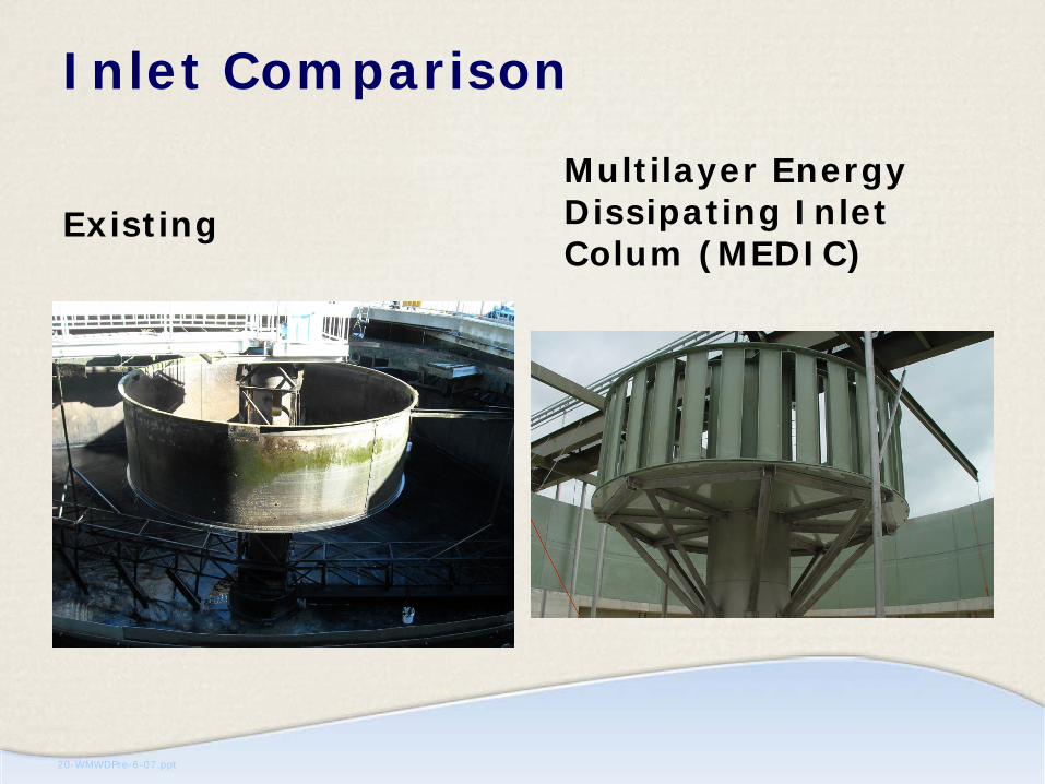
Inlet Comparison

ExistingMultilayer Energy Dissipating Inlet Colum (MEDIC)

20-WMWDPre-6-07.ppt

3D Model Results Summary of Model Runs

Clarifier Configuration

Operational Conditions Clarifier Performance

Clarifier Flow (mgd)

SOR (gpd/sf)

RAS Ratio (%)

MLSS (mg/L) SVI (mL/g)

Theoretical RAS Predicted

ESS (mg/L)Predicted

RAS (mg/L)(mg/L)Test Calibration 3.5 714 33 3,600 126 14,509 15 11,000

Existing Clarifier 2.5 510 33 3,250 110 13,000 7.1 10,821

Existing Clarifier 3.5 714 33 3,250 110 13,000 13.1 10,773

Existing Clarifier + Perimeter Effluent Weir

and Baffle

3.5 714 33 3,250 110 13,000 14.5 10,772

Existing Clarifier 4.5 918 33 3,250 110 13,000 83 10,183

Existing Clarifier 3.5 714 66 3,250 190 8,100 428 6,234

Existing Clarifier 3.5 714 100 3,250 190 6,500 1017 5,167

3-Layer MEDIC + Middle Feed Well

2.5 510 33 3,250 110 13,000 5.2 10,943

3-Layer MEDIC + Middle Feed Well

3.5 714 33 3,250 110 13,000 5.7 11,025

3-Layer MEDIC + Middle Feed Well

4.5 918 33 3,250 110 13,000 6.7 10,904

3-Layer MEDIC + Middle Feed Well

3.5 714 33 3,250 190 13,000 10.5 8,482

3-Layer MEDIC + Middle Feed Well

3.5 714 66 3,250 190 8,100 7.9 6,985

3-Layer MEDIC + Middle Feed Well

3.5 714 100 3,250 190 6,500 7.8 6,015

20-WMWDPre-6-07.ppt

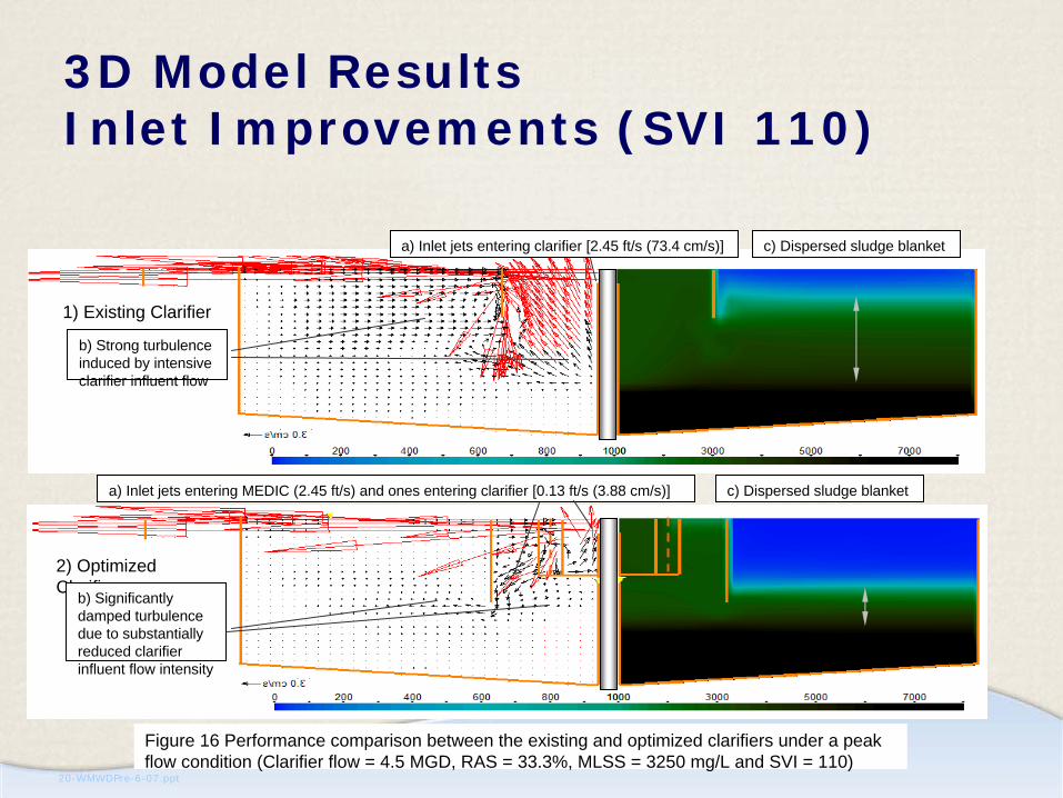
3D Model Results Inlet Improvements (SVI 110)

Figure 16 Performance comparison between the existing and optimized clarifiers under a peak flow condition (Clarifier flow = 4.5 MGD, RAS = 33.3%, MLSS = 3250 mg/L and SVI = 110)

1) Existing Clarifier

2) Optimized Clarifier

a) Inlet jets entering clarifier [2.45 ft/s (73.4 cm/s)]

a) Inlet jets entering MEDIC (2.45 ft/s) and ones entering clarifier [0.13 ft/s (3.88 cm/s)]

b) Strong turbulence induced by intensive clarifier influent flow

b) Significantly damped turbulence due to substantially reduced clarifier influent flow intensity

c) Dispersed sludge blanket

c) Dispersed sludge blanket

20-WMWDPre-6-07.ppt

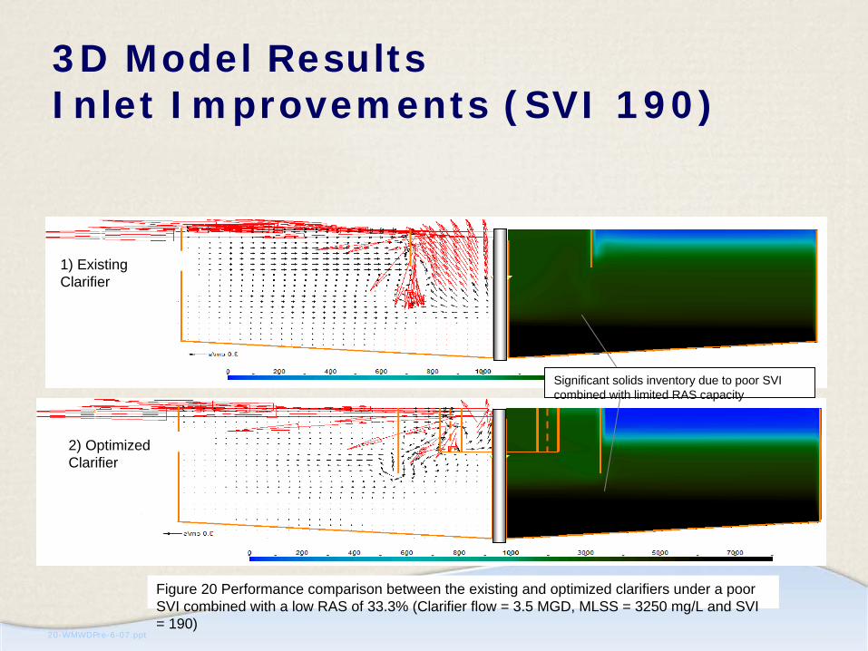
3D Model Results Inlet Improvements (SVI 190)

Figure 20 Performance comparison between the existing and optimized clarifiers under a poor SVI combined with a low RAS of 33.3% (Clarifier flow = 3.5 MGD, MLSS = 3250 mg/L and SVI = 190)

1) Existing Clarifier

2) Optimized Clarifier

Significant solids inventory due to poor SVI combined with limited RAS capacity

20-WMWDPre-6-07.ppt

Conclusions from 3D Modeling

• Optimized inlet would allow increase of safe operating flow from 3.5 to 4.5 mgd per clarifier with good SVI (110 mL/g)

(30% Increase)

• Optimized inlet would allow safe operation at 3.5 mgd per clarifier with poor SVI (190 mL/g) compared to 2.5 mgd with existing inlet

(40% increase)

20-WMWDPre-6-07.ppt

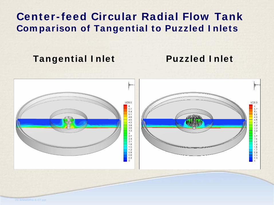
Center-feed Circular Radial Flow Tank Comparison of Tangential to Puzzled Inlets

Tangential Inlet Puzzled Inlet

20-WMWDPre-6-07.ppt

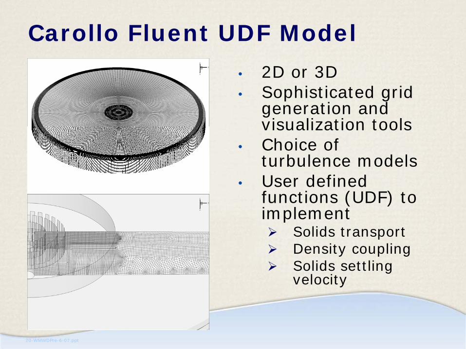
Carollo Fluent UDF Model• 2D or 3D • Sophisticated grid

generation and visualization tools

• Choice of turbulence models

• User defined functions (UDF) to implement

Solids transportDensity couplingSolids settling velocity

20-WMWDPre-6-07.ppt

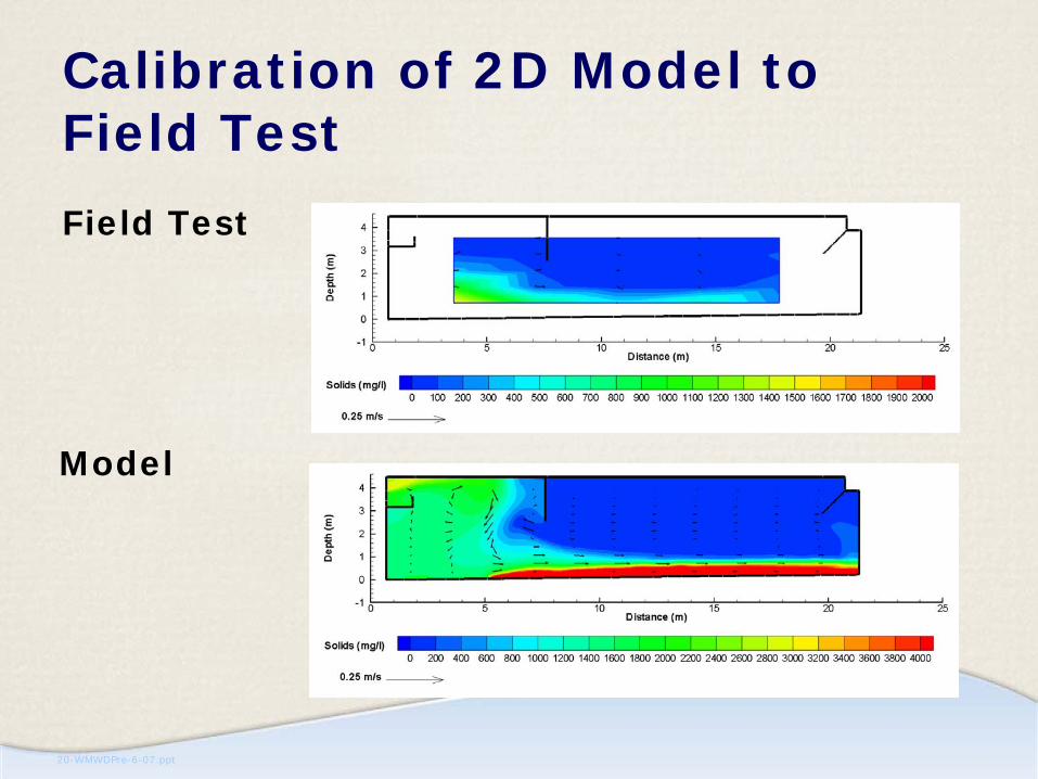
Calibration of 2D Model to Field TestField Test

Model

20-WMWDPre-6-07.ppt

Comparison of Tangential to Puzzled Inlets Inlet Velocities

Tangential Inlet Puzzled Inlet

20-WMWDPre-6-07.ppt

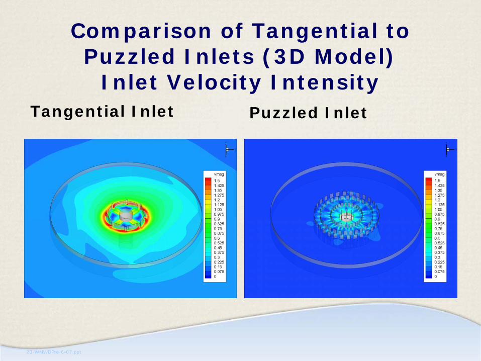
Comparison of Tangential to Puzzled Inlets (3D Model)

Inlet Velocity IntensityTangential Inlet Puzzled Inlet

20-WMWDPre-6-07.ppt

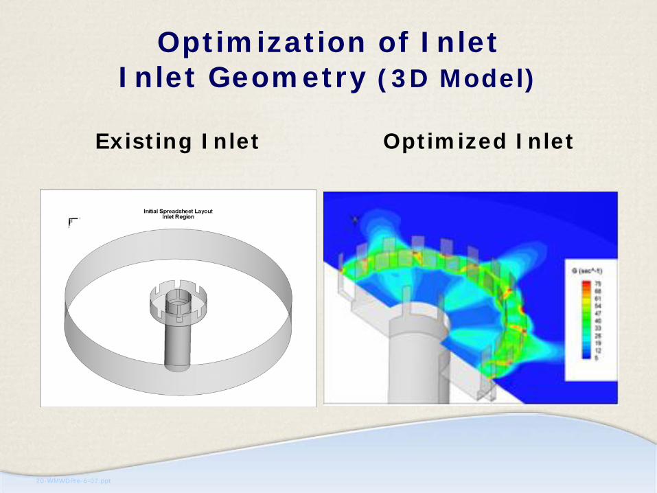
Optimization of Inlet Inlet Geometry (3D Model)

Existing Inlet Optimized Inlet

20-WMWDPre-6-07.ppt

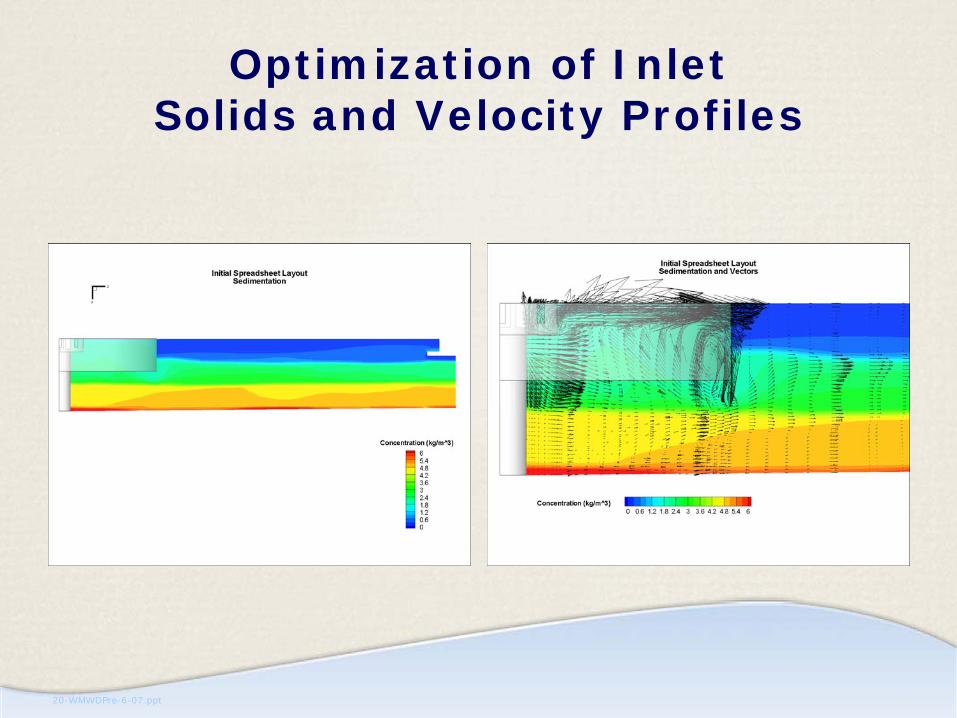
Optimization of Inlet Solids and Velocity Profiles

20-WMWDPre-6-07.ppt

Optimization of Inlet Comparison of Inlet Velocity and

EnergyExisting Inlet Optimized Inlet

20-WMWDPre-6-07.ppt

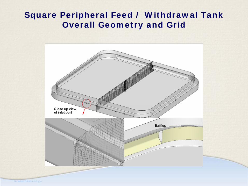
Square Peripheral Feed / Withdrawal Tank Overall Geometry and Grid

20-WMWDPre-6-07.ppt

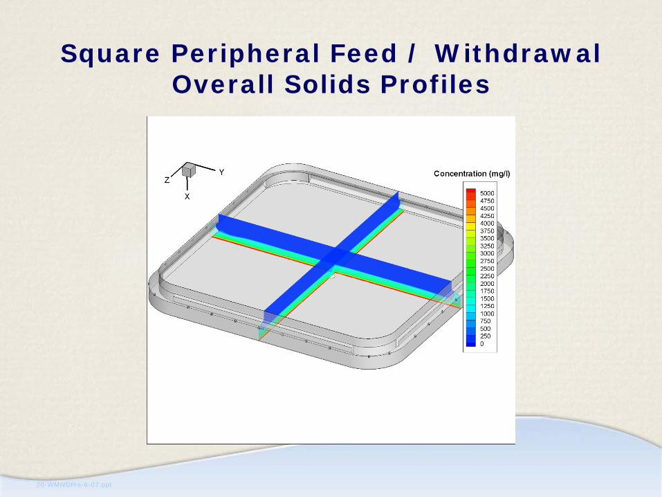
Square Peripheral Feed / Withdrawal Overall Solids Profiles

20-WMWDPre-6-07.ppt

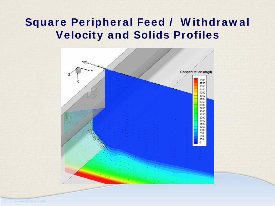
Square Peripheral Feed / Withdrawal Velocity and Solids Profiles

20-WMWDPre-6-07.ppt

Square Peripheral Feed / Withdrawal Sludge Blanket Level Topography

20-WMWDPre-6-07.ppt

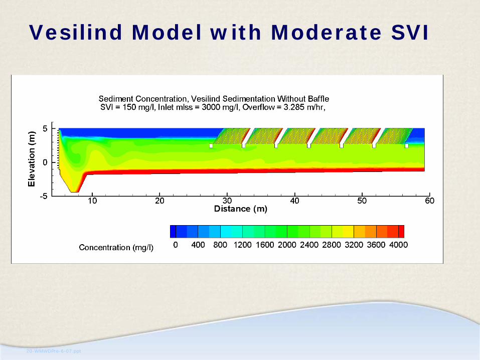
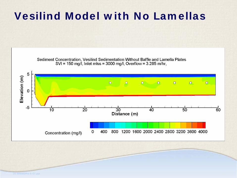
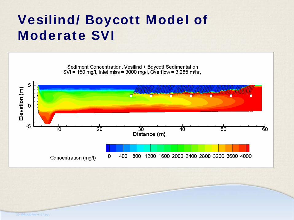
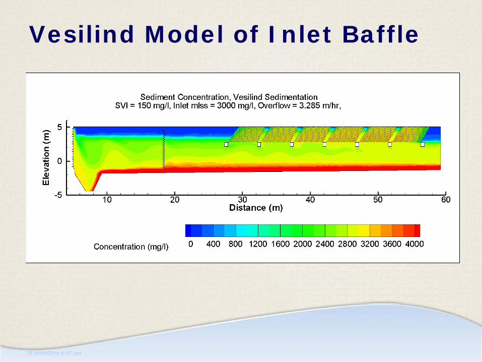
Rectangular Lamella Clarifier

• Carollo Fluent UDF Model

• 2D and 3D flow in and around the lamella plate modules

• Activated sludge clarifiers

• Two different settling models:

VesilindVesilind with Boycott in lamella zone

20-WMWDPre-6-07.ppt

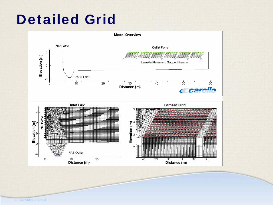
Detailed Grid

20-WMWDPre-6-07.ppt

Vesilind Model of Low SVI Condition

20-WMWDPre-6-07.ppt

Vesilind Model with Moderate SVI

20-WMWDPre-6-07.ppt

Vesilind Model with No Lamellas

20-WMWDPre-6-07.ppt

Vesilind/Boycott Model of Moderate SVI

20-WMWDPre-6-07.ppt

Vesilind Model of Inlet Baffle

20-WMWDPre-6-07.ppt

Conclusions• CFD models are well developed for

evaluation of sedimentation tanks• Each level of model has its place• Several important problems can only be

adequately evaluated using 3D modelsInlet designRadial flow / square shapeNon-symmetrical elements

• Commercial 3D CFD codes can be productively used but only with custom add-ons

20-WMWDPre-6-07.ppt

Questions?

Randal W. Samstag(rsamstag@carollo.com)

Ed A. Wicklein(ewicklein@carollo.com)