Maximum entropy autoregressive conditional heteroskedasticity modelI
Sung Y. Park a, Anil K. Bera b,∗a The Wang Yanan Institute for Studies in Economics, Xiamen University, Xiamen, Fujian 361005, Chinab Department of Economics, University of Illinois, 1206 S.6th Street, Champaign, IL 61820, USA
a r t i c l e i n f o
Article history:Available online 8 January 2009
JEL classification:C40C61G10
Keywords:Maximum entropy densityARCH modelsExcess kurtosisAsymmetryPeakedness of distributionStock returns data
a b s t r a c t
In many applications, it has been found that the autoregressive conditional heteroskedasticity (ARCH)model under the conditional normal or Student’s t distributions are not general enough to account for theexcess kurtosis in the data. Moreover, asymmetry in the financial data is rarely modeled in a systematicway. In this paper, we suggest a general density function based on the maximum entropy (ME) approachthat takes account of asymmetry, excess kurtosis and also of high peakedness. The ME principle is basedon the efficient use of available information, and as is well known, many of the standard family ofdistributions can be derived from the ME approach. We demonstrate how we can extract informationfunctional from the data in the form of moment functions. We also propose a test procedure for selectingappropriatemoment functions. Our procedure is illustratedwith an application to the NYSE stock returns.The empirical results reveal that the ME approach with a fewer moment functions leads to a model thatcaptures the stylized facts quite effectively.
There have been a number of theoretical and empirical studiesin the area of density estimation. Since complete informationabout the density function is not available, a parametric formis generally assumed before performing estimation. In non-parametric approach, estimated tail-behavior of the density, whichis of substantial concern in most financial applications, is notsatisfactory due to the scarcity of data in the tail part of thedistribution. If the density function is correctly specified, thenclassical maximum likelihood estimation preserves efficiencyand consistency. The true density, however, is not knownin almost all cases; therefore, an assumed density functioncould be misspecified. The main contribution of this paper isto show that how can one extract useful information about
I We are grateful to the editors Chung-Min Kuan and Yongmiao Hong, and twoanonymous referees for many pertinent comments and suggestions. We wouldalso like to thank the participants of the First Symposium on Econometric Theoryand Application (SETA) at the Institute of Economics, Academia Sinica, Taipei,Taiwan,May 18–20, 2005, and at some other conferences for helpful comments anddiscussions. In particular,we are thankful to Jin-ChuanDuan, Alastair R. Hall, GeorgeJudge, Nour Meddahi, Eric Renault, and Vicky Zinde-Walsh. However, we retain theresponsibility for any remaining errors. Financial support from the Research Board,University of Illinois at Urbana-Champaign is gratefully acknowledged.∗ Corresponding author. Tel.: +1 217 333 4596; fax: +1 217 244 6678.E-mail addresses: [email protected] (S.Y. Park), [email protected]
the unknown density from a given data by imposing somewell-defined moment functions in analyzing financial time-series data. By so doing one can reduce the degree of modelmisspecification considerably. We use the maximum entropydensity (MED) as conditional density function in the autoregressiveconditional heteroskedasticity (ARCH) framework. Since Engle’s(1982) pioneering work and its generalization by Bollerslev(1986), ARCH-type models have been widely used, and variousextensions have been suggested, primarily in two directions.First extension has concentrated on generalizing the conditionalvariance function. Second extension deals with the form of theconditional density function. Various non-normal conditionaldensity functions have been proposed to explain high leptokurticbehavior. Although these two extension are inter-related, in thispaper we concentrate on the second extension, namely, findinga suitable general form of the conditional density. If we imposecertain moment conditions, we can obtain normal, Student’st , generalized error distribution (GED) and Pearson type-IVdistribution through MED formulation. In this sense, our proposedmaximum entropy ARCH (MEARCH) model is a very general one.MEARCH model is quite related to other moment-based
estimation, such as generalized method of moments (GMM)and maximum empirical likelihood (MEL) estimation. All theseestimations could also be considered within estimating function(EF) approach, for example, see Bera et al. (2006). The purposeof this paper is twofold. First, we present the characterizationof MED, and show how, within an ARCH framework, our selectedmoment conditions capture asymmetry and excess kurtosis of
220 S.Y. Park, A.K. Bera / Journal of Econometrics 150 (2009) 219–230
financial data. Second, we introduce estimation procedure of theMEARCH model, and suggest moment selection criteria based onRao’s score test.The rest of the paper is organized as follows. In the next
section we present some basic characteristics of MED and discussestimation of a basic model. In Section 3, we propose our MEARCHmodel along with its estimation and the moment selection test.Section 4 provides an empirical application to the daily return ofNYSE with specific moment functions that generate a skewed andheavy tail distribution. The paper is concluded in Section 5.
2. Maximum entropy density
The maximum entropy density is obtained by maximizingShannon’s (1948) entropy measure
where the µj’s are known values. The normalization constraintcorresponds to j = 0 by setting φ0(x) and µ0 to 1. The Lagrangianfor the above optimization problem is given by
L = −
∫f (x) ln f (x)dx+
q∑j=0
λj
[∫φj(x)f (x)dx− µj
], (3)
where λj is the Lagrange multiplier corresponding the j-thconstraint in (2), j = 0, 1, 2, . . . , q. The solution to the aboveoptimization problem, obtained by simple calculus of variation,is given by [Zellner and Highfield (1988) and Golan et al. (1996),p. 36)]
f (x) =1
Ω(λ)exp
[−
q∑j=1
λjφj(x)
], (4)
where Ω(λ) is calculated by∫f (x)dx = 1, and can be
expressed in terms of the Lagrangian multipliers as Ω(λ) =∫exp
[−∑qj=1 λjφj(x)
]dx. Ω(λ) is known as the ‘‘partition
function’’ that converts the relative probabilities to absoluteprobabilities. In the maximization problem (1) and (2), φj(x) inthe moment constraint equation (hereafter, we call φ as momentfunction) is only function of data x. Due to this characteristicsof φj, we obtain simple exponential forms as a solution to themaximization problem. Since (4) belongs to exponential family,λj’s and φj(x)’s are the natural parameters and the correspondingsufficient statistics, respectively.We extend simple exponential solution forms to more general
exponential forms by introducing additional parameters, γ , in φj.Consider the following optimization problem,
The solution to (5) and (6), obtained by applying the sameLagrangian’s procedure, is the general exponential density
f (x) =1
Ω(λ, γ )exp
[−
q∑j=1
λjφj(x, γ )
], (7)
where Ω(λ, γ ) =∫exp
[−∑qj=1 λjφj(x, γ )
]dx. Thus, by adding
additional parameter γ to moment functions, the ME formulationprovides a more general family of distributions.The moment conditions can be interpreted as known prior
information, and using these we can achieve a least biaseddistribution by the ME principle. Suppose we have no priorinformation except for the normalization constraint, then thesolution is the uniform distribution which is a ‘‘perfect smooth’’density. If we have an additional information, say
∫xf (x)dx =
µ1 > 0, then the solution takes the form, f (x|λ1) = λ1 exp[−λ1x]where x ∈ [0,∞). With a further constraint, say
∫x2f (x)dx =
µ2, the associated solution is the normal distribution. In the nextsubsection, we discuss in detail the role of different momentconditions in some of the commonly used distributions, andalso suggest new densities by constructing and selecting certainmoment functions judiciously.All solutions are functions of Lagrangian multipliers which
represent marginal contribution (shadow price) of constraints tothe objective value. For example, suppose λ2 corresponding to∫x2f (x)dx = µ2 is estimated to be close to 0, then, there is littlecontribution of this moment constraint to the objective function.Consequently, the Lagrangian multiplier reflect the informationcontent of each constraint.
2.1. Maximum entropy characterization of thick tail, peakedness andasymmetry
Maximum entropy distribution has a very flexible functionalform. By choosing a sequence of moment functions φj(x), j =1, 2, . . . , q, we can generate a sequence of various flexible MEDfunctions. Many well-known families of distributions can beobtained as special cases of MED function. Kagan et al. (1973)provided characterization of many distributions, such as, the beta,gamma, exponential and Laplace distributions as ME densities. InTable 1, we present a number of well-known distributions undervarious moment constraints. These common distributions can beinterpreted in an information theoretic way that they are leastbiased density functions obtained by imposing certain momentconstraints which are inherent in the data. If we add more andmore moment constraints, the resulting density, f (x)will be moreunsmooth.Let us consider three moment functions x2, ln(γ 2 + x2) and
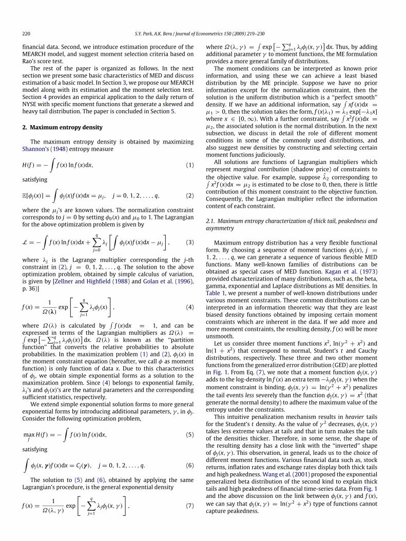
ln(1 + x2) that correspond to normal, Student’s t and Cauchydistributions, respectively. These three and two other momentfunctions from the generalized error distribution (GED) are plottedin Fig. 1. From Eq. (7), we note that a moment function φj(x, γ )adds to the log-density ln f (x) an extra term−λjφj(x, γ )when themoment constraint is binding. φj(x, γ ) = ln(γ 2 + x2) penalizesthe tail events less severely than the function φj(x, γ ) = x2 (thatgenerate the normal density) to adhere the maximum value of theentropy under the constraints.This intuitive penalization mechanism results in heavier tails
for the Student’s t density. As the value of γ 2 decreases, φj(x, γ )takes less extreme values at tails and that in turn makes the tailsof the densities thicker. Therefore, in some sense, the shape ofthe resulting density has a close link with the ‘‘inverted’’ shapeof φj(x, γ ). This observation, in general, leads us to the choice ofdifferent moment functions. Various financial data such as, stockreturns, inflation rates and exchange rates display both thick tailsand high peakedness. Wang et al. (2001) proposed the exponentialgeneralized beta distribution of the second kind to explain thicktails and high peakedness of financial time-series data. From Fig. 1and the above discussion on the link between φj(x, γ ) and f (x),we can say that φj(x, γ ) = ln(γ 2 + x2) type of functions cannotcapture peakedness.
S.Y. Park, A.K. Bera / Journal of Econometrics 150 (2009) 219–230 221
Table1
CharacterizationofsomecommondensitiesasMED.
Type
Momentconstraints
Correspondingformofthedensity,f(x)
Commonformofthedensityfunction,f(x)
Uniform
None
exp[ −λ0]
1b−a,
a≤x≤b,(b>a)
Exp.
∫ xf(x)dx=m(m>0)
exp[ −λ0−λ1x]
1 mexp[ −x m
] ,0≤x<∞
Normal
∫ xf(x)dx=µ
exp[ −λ 0
−λ1x−λ2x2]
1σ√2πexp[ −(x
−µ)2
2σ2
] ,−∞<x<∞
∫ (x−µ)2f(x)dx=σ2
Log-normal
∫ lnxf(x)dx=µ
exp[ −λ 0
−λ1lnx−λ2(lnx)2]
1σ√2πxexp[ −(ln
x−µ)2
2σ2
] ,0<x<∞
∫ (lnx−µ)2f(x)dx=σ2
Gen.exp.
∫ xi f(x)dx=µii=1,2,...N
exp[ −∑
N n=0λnxn]
exp[ −∑
N n=0λnxn]
−∞<x<∞
Doubleexp.
∫ |x−µ|f(x)dx=σ2
exp[ −λ 0
−λ1x−λ2|x|2]
C(θ)exp[ −|x−µ|/σ2]
−∞<x<∞
Gamma
∫ xf(x)dx=a(a>0)
exp[ −λ0−λ1x−λ2lnx]
1Γ(a)exp−xxa−1 ,
0<x<∞
∫ lnxf(x)dx=
Γ′(a)
Γ(a)
Chi-squaredwithνdf
∫ xf(x)dx=ν
exp[ −λ0−λ1x−λ2lnx]
12ν/2Γ(ν/2)exp−x/2xν/2−1 ,
0<x<∞
∫ lnxf(x)dx=
Γ′(1 2)
Γ(1 2)+ln2
Weibulla
∫ xa f(x)dx=1(a>0)
exp[ −λ0−λ1xa−λ2lnx]
axa−1exp[ −xa] ,
0<x<∞
∫ lnxf(x)dx=−γ/a
GED
∫ |x|νf(x)dx=c(ν)
exp[ −λ0−λ1|x|ν]
C(ν)exp[ |x|ν] ,
−∞<x<∞
Beta
∫ lnxf(x)dx=
Γ′(a)
Γ(a)−
Γ′(a+b)
Γ(a+b)
exp[ −λ0−λ1lnx−λ2ln(1−x)]
1B(a,b)xa−1 (1−x)b−1 ,
0<x<1
∫ ln(1−x)f(x)dx=
Γ′(b)
Γ(b)−
Γ′(a+b)
Γ(a+b)
Cauchy
∫ ln(1+x2)f(x)dx=2ln2
exp[ −λ 0
−λ1ln(1+x2)]
1π(1+x2),
−∞<x<∞
Student’st
∫ ln(r2+x2)f(x)dx=ln(r2 )+
Γ′(1+r2 2)
Γ(1+r2 2)−
Γ′(r2 2)
Γ(r2 2)
exp[ −λ 0
−λ1ln(r2+x2)]
Γ[(r2+1)/2]
√
πr2Γ(r2/2)
1(1+x2/r2)(r2+1)/2,
−∞<x<∞
Pearsontype-IV
∫ tan−1( x r) f(x)
dx=c 1(r)
exp[ −λ 0
−λ1tan−1( x r) −λ
2ln(r2+x2)]
K( 1+
x2 r2
) −m exp[ δtan
−1( x r)] ,
−∞<x<∞
∫ ln(r2+x2)f(x)dx=c 2(r)
GeneralizedStudent’st
∫ xi−2 f(x)dx=µii=3,4,...k
exp[ −λ 0
−λ1tan−1 (x r)−λ2ln(r2+x2)−∑ k i=3
λixi−2]
−∞<x<∞
∫ tan−1 (x r)f(x)=c 1(r)
∫ ln(r2+x2)f(x)=c 2(r)
Generalizedlog-normal
∫ xi−2 f(x)dx=µii=3,4,...k
exp[ −λ 0
−λ1lnx−λ2(ln(x))2−∑ k i=3
λixi−2]
0<x<∞
∫ lnxf(x)=c 1(r)
∫ (ln(x))2f(x)=c 2(r)
aγdenotestheEulerconstant.
222 S.Y. Park, A.K. Bera / Journal of Econometrics 150 (2009) 219–230
Fig. 1. Moment functions φj(x, γ ) representing thick tail.
Fig. 2. Moment functions φj(x, γ ) representing high peakedness.
To take account of high peakedness,we suggest functions ln(1+|x/r|p) and tan−1(x2/r2). In Fig. 2, these functions alongwith ln(1+x2) are plotted. We note that ln(1 + |x|1.3) and ln(1 + |x|0.7) havecusp at x = 0, while the Cauchy moment function ln(1+ x2) doesnot. In ln(1 + |x/r|p) the parameter p (<2) appears to capturepeakedness, while r takes account of the tail thickness. For p ≥2, the cusp behavior disappears, and for this case, both p and rtogether capture the tail behavior of the underlying distribution.Themoment function tan−1(x2) also captures high peakedness andpenalizes the tails less than that of ln(1+ x2).As is well known, financial data also displays asymmetry
(skewness), see for instance, Premaratne and Bera (2000). Momentfunctions, ln x, 0 < x < ∞, ln(1 − x), 0 < x < 1 and tan−1(x/γ ),−∞ < x < ∞ can capture asymmetry, and these are plotted inFig. 3. ln x and ln(1 − x) generates the beta distribution over therange 0 ≤ x ≤ 1; tan−1(x/γ ) is part of the moment functions ofthe Pearson type-IV density. E[ln x] = Γ ′(a)
Γ (a) is used as a momentcondition in gamma density and chi-squared is a special case ofgamma distribution when E[ln x] = Γ ′(1/2)
Γ (1/2) + ln 2 for 0 < x <∞.
Fig. 3. Moment functions φj(x, γ ) representing skewness.
Fig. 4. Moment functions φj(x, γ ) representing general skewness.
Premaratne and Bera (2005) used tan−1(x/γ ) to test asymmetry inleptokurtic financial data.In general, any odd function can serve as a moment function
to capture asymmetry. However, the benefits of a function liketan−1(x/γ ) are that it is bounded over the whole range and‘‘robust’’ to outliers. Chen et al. (2000) used sin(x) and βx/(1 +β2x2) with a specific value of β to test asymmetry. Tests based onsuch bounded functions will be more robust compared to thosebased on the third moment, i.e., moment function like x3 [formore on this, see, Premaratne and Bera (2005)]. Some robust-typefunctions that capture general skewness are plotted in Fig. 4.As we assign more andmore moment constraints in maximiza-
tion problem (1) and (2) or (5) and (6), the solution is likely tobecome more unsmooth (rough) functional if given moment con-straints are informative. There is a close relationships betweenMED and the penalization method. The ME method starts with avery smooth density and, adding more moment constraints, MEDis likely to havemore ‘‘roughness’’ butwith improved goodness-of-fit at the same time. Here we do not face the problem of selectingsmoothing parameter or the bandwidth. Instead, we need choose
S.Y. Park, A.K. Bera / Journal of Econometrics 150 (2009) 219–230 223
moment functions priori. On the other hand, a non-parametric ap-proach begins with a rough density (histogram), and then uses asmoothing procedure (such as selecting a proper bandwidth) tocontrol the balance between smoothness and goodness-of-fit. Gal-lant (1981), Gallant and Nychka (1987) and Ryu (1993) considered(semi-) non-parametric density estimators using flexible polyno-mial series approaches such as Fourier series, Hermite polynomialand any orthonormal basis. These approaches are useful to fit theunderlying density or functional form and to analyze asymptoticproperties of estimators since very high orders of polynomial se-ries can be easily considered. However, if one can select only afew informative functions that explain underlying density enoughinstead of using high orders of polynomials, the complexity andcomputational burden can be significantly reduced, and, more-over, some valuable interpretation can be made using the selectedinformative functions.
2.2. Methods of estimation
When µj’s are unknown in (2), the maximum likelihood (ML)estimates are the same as ME estimates when µj’s are replacedby their consistent estimates 1T
∑Tt=1 φj(xt), j = 1, 2, . . . , q. Since
exponential family distributions have a uniqueML solution, theMEsolution is also unique, if it exists. However, whenwe have generalmoment conditions [as in (6)], thenwe have to consider estimationof unknown parameter γ . Usually, this estimation problem canbe solved by estimating saddle point of the objective functionproposed by Kitamura and Stutzer (1997) and Smith (1997).Let us rewrite (6) as∫[φj(x, γ )− Cj(γ )]f (x)dx
=
∫ψj(x, γ )f (x)dx = 0, j = 1, 2, . . . , q,
whereψj(x, γ ) = φj(x, γ )−Cj(γ ). The profiled objective functionis obtained by substituting (7) to the Lagrangian (3)
ln∫exp
[−
q∑j=1
λjψj(x, γ )
]dx. (8)
ME estimators of the parameters γ and λ are the solution offollowing saddle point problem
γME = argmaxγln∫exp
[−
q∑j=1
λjψj(x, γ )
]dx,
where λ(γ ) is given by
λ(γ )ME = argminλln∫exp
[−
q∑j=1
λjψj(x, γ )
]dx.
Since the profiled objective function (8) has the exponentialform it is relatively easy to calculate first order derivatives.However, Cj(γ ) could be complicated in some case or even, maynot have analytic form. In such a case, Cj(γ ) can be substituted bythe sample moment of φj(x, γ ). Thus, we consider the followingnon-linear equations:∫φj(x, γ )f (x|λ, γ )dx =
1T
T∑t=1
φj(xt , γ ), j = 1, 2, . . . q.
We can express (8) as
ln∫exp
[−
q∑j=1
λjφj(x, γ )+q∑j=1
λjCj(γ )
]dx
= ln
[exp
[q∑j=1
λjCj(γ )
]·
∫exp
[−
q∑j=1
λjφj(x, γ )
]dx
]
=
q∑j=1
λjCj(γ )+ ln∫exp
[−
q∑j=1
λjφj(x, γ )
]dx.
Since from (4) ln∫exp
[−∑qj=1 λjφj(x, γ )
]= lnΩ(λ, γ ) the
above expression can be simplified asq∑j=1
λjCj(γ )+ lnΩ(λ, γ ). (9)
From (7) the log-likelihood function is given by
l(λ, γ ) = −T lnΩ(λ, γ )−q∑j=1
λj
T∑t=1
φj(xt , γ ). (10)
From (9) and (10) it is clear that profiled objective function isthe same as −(1/T )l(λ, γ ). Thus, the first order condition for theME principle and the ML principle are the same under the generalmoment problem. However, the second order conditionmay differbetween those principles because there exist restrictions that theLagrange multipliers are the functions of γ in the ME problem.However, in the ML problem, λj is not a function of γ because(1/T )
∑Tt=1 φj(xt , γ ) does not affect the form of the solution (7).
3. Maximum entropy GARCHmodel
Various ARCH-type models under the assumption of non-normal conditional density have been proposed to explainleptokurtic and asymmetric behavior of financial data.We proposeto use flexible ME density to capture such stylized facts, andconsider the following model:yt = mt(xt; ζ )+ εt , t = 1, 2, . . . , T ,where mt(·) is the conditional mean function, xt is a K × 1 vectorof exogenous variables and ζ is a vector of parameters. We assumethat εt |Ft−1 ∼ g(0, ht), where g(·) is the unknown densityfunction of εt conditional on the set of past information Ft−1, andht = α0 +
∑pj=1 αjε
2t−j +
∑sj=1 βjht−j.
Following (7), we can write the density function of thestandardized error term ηt (= εt/
√ht ) in a general MED form as
f (ηt) =1
Ω(λ, γ )exp
[−
q∑j=1
λjφj(ηt , γ )
], (11)
whereφj(ηt , γ ), j = 1, 2, . . . , q, denote themoment functions.Wewill term ARCHmodel with conditional density f (εt |Ft−1) impliedby the aboveMED f (ηt) as themaximum entropy ARCH (MEARCH)model. The (conditional) quasi-log-density function of εt is givenby
lQMEt (θ) = − lnΩ(λ, γ )
−
q∑j=1
λjφj
(yt − x′tζ√ht
, γ
)−12ln ht , t = 1, . . . , T ,
where θ = (α′, β ′, ζ ′, λ′, γ ′)′ ∈ Θ , and hence the quasi-log-likelihood function is
lQME(θ) =T∑t=1
lQMEt (θ)
= −T lnΩ(λ, γ )−T∑t=1
q∑j=1
λjφj
(yt − x′tζ√ht
, γ
)
−12
T∑t=1
ln ht . (12)
224 S.Y. Park, A.K. Bera / Journal of Econometrics 150 (2009) 219–230
The scores corresponding to the quasi-log-likelihood for ARCHregression model are
∂ lQME(θ)∂α
=
T∑t=1
[12ht
∂ht∂α
[q∑j=1
λjφ′
j (·)εt
h1/2t− 1
]], (13)
∂ lQME(θ)∂ζ
=
T∑t=1
[q∑j=1
λjφ′
j (·)x′th1/2t
+12ht
∂ht∂ζ
[q∑j=1
λjφ′
j (·)εt
h1/2t− 1
]], (14)
∂ lQME(θ)∂λj
= −T∂ lnΩ(λ, γ )
∂λj−
T∑t=1
φj
(yt − x′tζ√ht
, γ
), (15)
∂ lQME(θ)∂γ
= −T∂ lnΩ(λ, γ )
∂γ−
T∑t=1
q∑j=1
λj
∂φj
(yt−x′t ζ√ht, γ)
∂γ, (16)
where φ′j (·) = ∂φj(η, γ )/∂η. The quasi-log-likelihoodspecification (12) is related to other semi-nonparametric ARCHapproaches. In parametric model, the score function is theoptimal estimating function (EF) (Godambe, 1960). If underlinedconditional density is correctly specified, then Eqs. (13)–(16) arethe optimal estimating functions (EFs). Li and Turtle (2000) derivedthe optimal EFs for ARCH model as
`∗1 = −
T∑t=1
∂ht∂α
h2t (γ2t + 2− γ 21t)g2t , (17)
`∗2 = −
T∑t=1
∂x′t ζ∂ζ
htg1t +
T∑t=1
h1/2t γ1t∂x′t ζ∂ζ−
∂ht∂ζ
h2t (γ2t + 2− γ 21t)g2t , (18)
where g1t = yt − x′tζ , g2t = (yt − x′tζ )
2− ht − γ1th
1/2t (yt − x′tζ ),
γ1t =E[(yt−x′t ζ )
3|Ft−1]
h3/2t, and γ2t =
E[(yt−x′t ζ )4|Ft−1]
h2t− 3. (17) and
(18) are actually the same as GMM moment conditions attainableby optimal instrumental variables. There is no priori distributionalassumption for yt conditional on Ft−1 in the EF approach. Underthe conditional normality assumption, γ1t = 0, and γ2t = 0,Eqs. (17) and (18) are identical to the first order condition of Engle(1982) [Equation (7), p. 990] up to a sign change. We can relateour approach to robust estimation through the influence function.Let us considerM-estimation thatminimizes
∑Tt=1 ρ(ηt , θ), where
ηt = (yt − x′tζ )/√ht , and define the influence function as
−ν(η, θ)/E[∂ν(η, θ)/∂η], where ν(η, θ) = ∂ρ(η, θ)/∂η [seeMcDonald and Newey (1988)]. If ρ(·) is negative of the naturallogarithm of the true density, then we have the ML estimator ofθ . Function ν(·) measures the influence that η will have on theresulting estimators. For the ME density in (11), the function ν(·)is
ν(η, θ) =
q∑i=1
λi∂φi(η, θ)
∂η. (19)
For N(0, 1) density, λφ(η, θ) = 12η2 and hence ν(η, θ) = η
which is unbounded. Li and Turtle (2000) did not assume anyparticular conditional density and followed a semi-parametricmethod. In their EFs (17) and (18), the γ1t and γ2t shouldbe specified in some arbitrary way. They noted that since theorthogonality of g1t and g2t holds for any γ2t , an approximate valuefor γ2t might be used to give near optimal estimating functions l∗1and l∗2 . If the underlying density is Cauchy, the parameters cannotbe estimated consistently by EF approach due to the non-existenceof moments. Our MEARCH approach, however, can be used since
the moment condition, E[ln(1+ x2)
]= 2 ln 2, generates Cauchy
distribution and the associated influence function ν(η, θ) =λ(2η)/(1 + η2) is bounded. Therefore, careful choice of momentfunction φ(·) can lead to robust estimation.
3.1. Estimation
For ARCH-type models, the standardized error term, ηt =εt/√ht , should have mean 0 and variance 1. However, the MED
of ηt given in (11) may not have this property. For convenience, werewrite (11) as
f (ηt) = C−1 exp
[−
q∑j=1
λjφj(ηt , γ )
], (20)
where C denotes normalizing constant and the parameters vectorγ ≡ [γ ′p : γs]
′, where γs denotes a scale parameter. Suppose thedensity (20) is such that E(ηt) = µ and V(ηt) = σ 2. If we defineut = (ηt − µ)/σ , then ut ∼ (0, 1) and ηt = σut + µ. Due to thetransformation ut = (ηt − µ)/σ , the density (20) in terms of εtchanges to
fε(εt) = C−1σ1√htexp
[−
q∑i=1
λiφi
(σεt√ht+ µ, γ
)]. (21)
In (21), the scale parameter γs, however, will not separately beidentified within an ARCH framework. To make the density freeof γs, let us define ηt = ηt/γs, so that E(ηt) = µ/γs = µ andV(ηt) = σ 2/γs
2= σ 2. The density function of ηt , f (ηt) can be
written as
f (ηt) = C−1 exp
[−
q∑i=1
λiφi(ηt , γp
)]. (22)
An ‘‘equivalent’’ density is obtained by substituting µ = γsµand σ = γsσ in the (21) as
fεt (ε) = C−1γs
σ√htexp
[−
q∑i=1
λiφi
(γsσ εt√ht+ γsµ, γ
)]
= C−1σ√htexp
[−
q∑i=1
λiφi
(σ εt√ht+ µ, γp
)]. (23)
The quasi-log-likelihood function corresponding to the density(23) can be written as
l(θ) =T∑t=1
ln g
(εt
h1/2t
)−12
T∑t=1
ln ht (24)
= −T ln C + T ln σ
−
T∑t=1
q∑i=1
λiφi
(σ εt√ht+ µ, γp
)−12
T∑t=1
ln ht , (25)
where θ = (α′, β ′, ζ ′, λ′, γ ′p)′ and g(·) is the quasi-density
function of ut given by
g(ut) = C−1σ exp
[−
q∑i=1
λiφi(σut + µ, γp
)]. (26)
Since φi(·)’s in (25) are not predetermined but are selectedfrom a variety of moment functions to the underlying density, onecannot guarantee C−1, µ, and σ to have analytic forms. Therefore,in practical applications these are computed using numericalintegration.Following our discussion in Section 2 that the first order
conditions for maximizing entropy and the likelihood function are
S.Y. Park, A.K. Bera / Journal of Econometrics 150 (2009) 219–230 225
the same under general moment problem, we obtain ourparameter estimator by maximizing (25). A range of numericaloptimization techniques can be used to maximize (25). Weadapted the Broyden, Fletcher, Goldfarb and Shannon (BFGS)algorithm. For computational convenience, the derivatives arecomputed numerically. We will denote our estimator as θQMLE .Lee and Hansen (1994) and Lumsdaine (1996) showed consistencyand asymptotic normality for the QMLE under ‘‘conditionalnormal’’ GARCH model. Lee and Hansen (1994) established theseresults under the assumption that ut is a stationary martingaledifference sequence with E|ut |κ < ∞ with some κ ≤ 4.Ling and McAleer (2003) proved consistency and asymptoticnormality of QMLE under the second-order moments of theconditional distribution and the finite fourth-order moments ofthe unconditional distribution of ut . We assume that our modelsatisfies these conditions. The limiting distribution of θQMLE isgiven by√T(θQMLE − θ0
)−→
d N(0, A0T
−1B0TA
0T−1),
where θ0 is the quasi-true parameter, A0T = −T−1E
(∂2 l(θ0)∂θ∂θ ′
), and
B0T = T−1E
(∂ l(θ0)∂θ
∂ l(θ0)∂θ ′
). When our ME density function coincides
with the true density, then θQMLE ≡ θMLE and we have√T(θQMLE − θ0
)−→
d N(0, B0T
−1).
Instead of maximizing (25) with respect to all the parameters,a computationally less burdensome procedure would be a two-step approach of estimation. In the first-step, using some initialconsistent estimates (such as, obtained bymaximizing a likelihoodfunction assuming normality) of the conditioned mean and
variance parameters, we can obtain ηt = εt/
√ht and then fit
a ME density to ut = (ηt − µ)/σ , using proposed methodsin Section 2. In the second-step, fixing the estimated density,g(·) in (24), we can maximize quasi-log-likelihood function withrespect to the set of parameter of interest. Engle and González-Rivera (1991) suggested such an approach, where in the first-step, they used a non-parametric method of density estimation.However, based on their simulation results, they noted (p. 350):‘‘When conditional distribution is Student’s t , we cannot find anygain. We suspect that this poor performance come from the poornon-parametric estimation of the tails of the density.’’ We cantake care of the tail part of distribution by choosing momentfunctions targeting the tail area of the density. Another problemwith the two-step procedure is that for a GARCH model witha general distribution that takes care of asymmetry and excesskurtosis, the underlying information matrix may not be block-diagonal between the conditional mean and variance parametersand the distributional parameters. Therefore, for a such a model,complete adaptive estimation is not possible. Also for this case,the usual standard errors of the parameters estimated by two-stepmethod will not be consistent, as noted by Engle and González-Rivera (1991, p. 352). Therefore, for efficient estimation and validinference, it is necessary to consider the joint estimation of all theparameters.
3.2. Moment selection test
As we discussed earlier, Lagrange multipliers provide marginalinformation of the constraints, and therefore, λj should be veryclose to zero if its associated moment function does not conveyany valuable information. Now we derive a statistic for testingH0j : λj = 0 using Rao’s score (RS) principle. Detailed derivation isgiven in the Appendix.
Note that C , σ and µ in the log-likelihood function l(θ) given in(25) are functions of the parameter vector θ = (α′, β ′, ζ ′, λ′, γ ′p)
′.The first derivatives of l(θ)with respect to λj is given by
dλj = −T∂ ln C(θ)∂λj
+ T∂ ln σ (θ)∂λj
−
T∑t=1
φj
(σ (θ)εt√ht+ µ(θ)
)−
T∑t=1
∆j, (27)
where
∆j =
q∑i=1
λi
[φ′j
(σ (θ)εt√ht+ µ(θ)
)×
(∂σ (θ)
∂λj
εt√ht+∂µ(θ)
∂λj
)],
and for notational convenience, from now on the parameter vectorγp is subassumed within φ(·).The score function (27), under λj = 0, reduces to [the details
2φj(η)], ϕj = Eg0 [φj(u)],and ξj = Eg0 [∆j] denoting each subscript represents a particulardistribution with which the expectation is taken. Distributions,f0(η) and g0(u) are given by
f0(η) =
exp
[−
∑i=1,2,...,q\j
λiφi(η)
]∫exp
[−
∑i=1,2,...,q\j
λiφi(η)
]dη
, (28)
g0(u) =
exp
[−
∑i=1,2,...,q\j
λiφi
(ω1/2v u+ ωm
)]∫exp
[−
∑i=1,2,...,q\j
λiφi
(ω1/2v u+ ωm
)]du
, (29)
where∑i=1,2,...,q\j mean summation over i = 1, 2, . . . , j −
1, j + 1, . . . , q. We write the score statistic for testing λj = 0 asRj(θ) = d0λj/T , which is given by
Rj(θ) =(ϕj + ξj
)−1T
T∑t=1
φj
(ω1/2v εt√ht+ ωm
)−1T
T∑t=1
∆j.
= Eg0[φj(u)+ ∆j
]−1T
T∑t=1
[φj
(ω1/2v εt√ht+ ωm
)+ ∆j
].
Therefore, the test can be viewed as the difference betweenpopulation mean relating to the j-th moment function and itssample counterpart. Since ϕj, ξj, ωm, ωv , and ∆j in Rj(θ) includeexpectation operator, thosewill depend on the distributions underthe null hypothesis as given in (28) and (29). When f0(η) is
226 S.Y. Park, A.K. Bera / Journal of Econometrics 150 (2009) 219–230
Fig. 5. NYSE return data and non-parametric kernel density. Notes: Usual Gaussian kernel is used for estimating non-parametric density in which rule-of-thumb bandwidth(Silverman, 1984) is 0.1035.
symmetric around 0, thenEf0 [φi(η)] = 0 ifφi(η) is an odd functionand has point symmetric property at vertex 0. For an even functionthe expectation is not zero. Examples of odd and point symmetricfunctions are tan−1(η), η/(1 + η2), sinh−1(η), and sin(η), whileln(1+ η2), ln(1+ |η|p), tan−1(η2), and cos(η) are even functions.Premaratne and Bera (2005) developed a test of the form Rj(θ)for testing asymmetry under heavy tails distribution. They usedPearson type-IV density function under the alternative hypothesis.Thus, under the null, their distribution becomes Pearson type-VII which is symmetric around 0 and also includes Student’s tas a special case. It can be easily checked that their Rj(θ) =−1T
∑Tt=1 tan
−1(ηt/r) and E[tan−1(ηt/r)] = 0 under symmetry.An operational form of Rao’s score (RS) statistic would be
RSj = T ·R2j (θ)
V,
where θ is the MLE of θ and V is an consistent estimator ofasymptotic variance of
√T · Rj(θ). Under the null hypothesis, H0 :
λj = 0, RSj is asymptotically distributed as χ21 . We obtain V bybootstrap approach, and the bootstrap score test statistic is givenby
RSjB = T ·R2j (θ)
VB, (30)
where VB denotes the variance of Rj(θ) calculated by bootstrapmethod. Under the null hypothesis, as B → ∞, RSjB isasymptotically distributed as χ21 . For finite B, RSjB is asymptoticallydistributed as Hotelling’s T 2 with (1, B− 1) degrees of freedom, inshort T 21,B−1 [see Dhaene and Hoorelbeke (2004)].
4. Empirical application
To illustrate the suitability of ourmethodology to financial data,we consider an empirical application of MEARCH model using thedaily prices of NYSE, from Jan.1, 1985 to Dec. 30, 2004, a totalof 5218 observations obtained from the Datastream. To achievestationarity, we transform the indices prices into returns, rt =[ln St/St−1]×100, where St is the price index at time t . The returnsdata and a corresponding non-parametric density are plotted inFig. 5. The data plot clearly shows that there is a high degree ofclustering (conditional heteroskedasticity) and the estimated non-parametric density indicates high degree of non-normality withthick tails and high peakedness. The sample kurtosis, skewness andJarque and Bera (JB) normality test statistics are 55.89,−2.43 and613,269, respectively, and indicate not only high excess kurtosis
but also distinct negative skewness. Ljung-Box (LB) test statisticsfor residuals from an AR(1) model at lags 12 days using theseries (Q ) and its squares (Q 2), cubes (Q 3) and fourth-power (Q 4)are 22.87, 424.93, 42.31 and 7.20, respectively. It appears thatAR(1) model can take account of part of autocorrelation in thedata. Very high values of Q 2 indicate non-linear dependence andstrong presence of conditioned heteroskedasticity. The Q 3 and Q 4statistics measure higher order dependence and some changes inthe third and fourth moments over time but these changes are notas strong as for the time varying second moment as evident fromthe high values of Q 2. To explain such behaviors of stock returndata, we need to consider a model which captures distributionalcharacteristics and dynamic moment structure simultaneously.For the testing and selecting different moment functions, we
start with two separate ME densities as distributions under therespective null hypothesis. The first density corresponds to themoment function ln(1 + η2) = ln(1 + (η/r)2) and as notedearlier, this is the Pearson type VII distribution which includesStudent’s t as a special case. The second density is implied by themoment function ln(1 + |η|p) and reduces to the first one whenp = 2. Since the results of our tests based on statistic (30) withdifferent bootstrap sample sizes B = 50, 100, 150 and 200 aresimilar, we report the results only for B = 100 (Table 2). Whenthe null density comes from the moment function ln(1 + η2),the Lagrange multipliers corresponding to tan−1(η2), sinh−1(η)and tan−1(η) are all highly significant. As noted earlier, tan−1(η)represents high peakedness, and sinh−1(η) and tan−1(η) captureasymmetry. Our test results indicate that these three momentfunctions take account of certain data characteristics and conveysome additional information after we have already started withthe moment function ln(1+ η2), i.e., the Pearson type VII density.On the other hand, none of the additional Lagrange multipliers aresignificant when we test the null density implied by the momentfunction ln(1 + |η|p) (with maximum likelihood estimate, p =1.3978). This function behaves like a ‘‘sufficient’’ moment functionin the sense that once we start with ln(1 + |η|p), the additionalmoment functions do not throwany further light on the underlyingdensity. It is as if ln(1+|η|p) exhausts all the available information(in the sample) that is relevant for estimating the density function.Wenowuse these test results and estimate the AR(1)-GARCH(1,
1)modelwith variousMEdensities.We consider the threemomentfunctions one-by-one (in addition to ln(1 + η2)) for which theassociated Lagrange multipliers were significant (see Table 2). Theestimation results are reported in Table 3. It is clear that additionalmoment functions increase the log-likelihood value substantiallyand make the model selection criteria AIC and SIC values moreattractive. We should add that the moment function ln(1 + |η|p)where p appears as an additional parameter, by itself performs
S.Y. Park, A.K. Bera / Journal of Econometrics 150 (2009) 219–230 227
Table 2Moment function selection test results with bootstrap sample size B = 100.
Notes: (i) and (ii) denote null density corresponds to the moment function ln(1 + η2) and ln(1 + |η|p), respectively. P-values are given in the parentheses and calculatedusing asymptotic χ21 distribution. 1% critical values of Hotelling’s T
2 are T 21,49: 7.181, T21,99: 6.898, T
21,149: 6.808, T
21,199: 6.764., respectively.
* Indicates statistical significance at the 1% level.
Table 3Estimation with different moment functions.
(i) (i) & (i) & (i) & Model 1 Model 2 Model 3 Model 4ln(1+ η2) tan−1(η2) sinh−1(η) tan−1(η)
Note: Standard errors are given in the parentheses.
extremely well. Also, as we discussed in Section 2.1, p = 1.3978 <2 captures the peakedness of the distribution. This encourages usto test various combinations of moment functions and estimatemodels with different sets of moment functions. To conserve spacewe do not report all the test and estimation results but these canbe obtained from us on request. In the right panel of Table 3,we present results from four models under several combinationsof moment functions for which the Lagrange multipliers weresignificant. The moment functions used in these models are quiteclear from the lower part of the Table 3; for example, the Model 1corresponds to moment function ln(1+ |η|p).Model 4, apparently the ‘‘best’’ model, includes six moment
functions for which all the Lagrange multipliers are highlysignificant. Performance of Models 2 and 3 are almost identical asthe moment functions tan−1(·) and sinh−1(·) have similar shape(see Fig. 4), and aswe shall also see in Figs. 6 and 7. Using our earlierdiscussion it is tempting to say that ln(1+ η2) exclusively explainsexcess kurtosis, tan−1(η2) captures high peakedness, and tan−1(η)
and other functions take care of asymmetry, etc. However, thesemoment functions are not orthogonal and therefore, when manyare present in a single ME density, we need to consider theircombined effect.It is interesting to compare above estimation results to those
of GARCH models based on some other general parametricdensity functions used in the current literature: standard normal;Student’s t (Bollerslev, 1987); skewed-t (Fernández and Steel,1998; Lambert and Laurent, 2001); and inverse hyperbolic sine(IHS) [Hansen et al. (2000)]. The values of log-likelihood functionsand model selection criteria (AIC and SIC) for those models arereported in Table 4. We note that, in terms of goodness-of-fit,Model 4 achieves the levels of some of the very general standarddistributions quite easily.In Figs. 6 and 7 we plot, respectively, the conditional densities,
and the influence functions ν(·), computed using the formula (19)for our four models (presented in Table 3). Density correspondingto Model 4 is very close to the non-parametric density based on
228 S.Y. Park, A.K. Bera / Journal of Econometrics 150 (2009) 219–230
Fig. 6. Density estimates for the standarized residuals of the final models. Notes: QMLE denotes usual Gaussian kernel density using Scott’s (1992) optimal bandwidth(0.1534) for standardized residual from the estimated GARCH model under conditional normality.
the standardized residuals of the estimated GARCH model underconditional normality (QMLE). All the four influence functions arebounded, and as expected it is hard to distinguish the lines forModels 2 and 3. The influence function corresponding to theModel4 has the least variation and comes out to be the best. Thus, aftera series of estimations and tests, our maximum entropy approachleads to a model that captures stylized facts quite effectively.
5. Concluding remarks
In this paper, we provide a generalization of GARCH modelby incorporating MED as the underlying probability distribution.We characterize MED and discuss various moment functionsthat are suitable to capture excess kurtosis, asymmetry and highpeakedness generally observed in financial data. We devise a testto select appropriate moment functions. Our empirical resultsdemonstrate that the suggested MEARCH model is quite usefulin capturing the behavior of the data. Many other momentfunctions and their mixtures could be chosen to generate evenmore flexible density. Our procedure is quite different fromthose that use certain non-normal densities. Those densities havefixed forms and not amenable to easy modification. Ours is acompletely flexible procedure where various moment functionsare selected based on the information available from the data.The approach is also constructive than a (semi-) non-parametricone using orthonormal series in the sense that the ME modelprovides a highly parsimonious model. The extension to themultivariate MEARCH model is of particular interest since manyempirical works deal with the multivariate GARCH models suchas Bollerslev’s (1990) constant conditional correlation and Engle’s(2002) dynamic conditional correlation models [for a review
S.Y. Park, A.K. Bera / Journal of Econometrics 150 (2009) 219–230 229
of these models see Bauwens et al. (2006)]. Kouskoulas et al.(2004) and more recently, Wu (2007) explored the computationalmethods and properties formultivariateMEDunder the arithmeticand Legendre series moment constraints, respectively. It wouldbe useful to extend their approaches to the general momentsconstraints that we suggest.
Appendix. Derivation of the moment selection test
We start with the log-likelihood function (25)
l(θ) = −T ln κ(θ)
−
T∑t=1
q∑i=1
λiφi
(σ (θ)εt√ht+ µ(θ)
)−12
T∑t=1
ln ht , (A.1)
where κ(θ) = C(θ)−1σ (θ) in the density of u given in (26). Forconvenience κ(θ) can be represented as
κ(θ) =
∫exp
[−
q∑i=1
λiφi(σ (θ)u+ µ(θ))
]du.
Note that κ(θ), µ(θ), and σ (θ) are also function of Lagrangemultiplier, λj for j = 1, 2, . . . , q, and µ(θ) =
∫ηf (η)dη and
σ (θ) =(∫(η − µ)2 f (η)dη
)1/2.
The score function of dλj is
dλj =∂ l(θ)∂λj= −T
∂ ln κ(θ)∂λj
−
T∑t=1
[φj
(σ (θ)εt√ht+ µ(θ)
)+
q∑i=1
λi∂φi(·)
∂λj
]
= −T∂ ln κ(θ)∂λj
−
T∑t=1
φj
(σ (θ)εt√ht+ µ(θ)
)−
T∑t=1
∆j, (A.2)
where
∆j =
q∑i=1
λiφ′
i
(σ (θ)εt√ht+ µ(θ)
)(∂σ (θ)
∂λj
εt√ht+∂µ(θ)
∂λj
)with φ′i (·) as the derivative of φi(·). Belowwe obtain ∂ ln κ(θ)/∂λj,∂µ(θ)/∂λj and ∂σ (θ)/∂λj to get explicit expression of the scoredλj .Since µ(θ) = C(θ)−1
∫η exp
[−∑qi=1 λiφi(η)
]dη.
∂µ(θ)
∂λj=∂ C(θ)−1
∂λj
∫η exp
[−
q∑i=1
λiφi(η)
]dη
− C(θ)−1∫ηφj(η) exp
[−
q∑i=1
λiφi(η)
]dη. (A.3)
Using the expression of f (η) in (22)∫f (η)dη =
∫1
C(θ)exp
[−
q∑i=1
λiφi (η)
]dη = 1.
By differentiating this with respect to λj, we have the identity
1
C(θ)2∂ C(θ)∂λj
∫exp
[−
q∑i=1
λiφi(η)
]dη
+ C(θ)−1∫exp
[−
q∑i=1
λiφi(η)
]φj(η)dη = 0. (A.4)
Using this identity, ∂ C(θ)−1/∂λj in (A.3) can be expressed as
∂ C(θ)−1
∂λj=
C(θ)−1∫φj(η) exp
[−
q∑i=1λiφi(η)
]dη
∫exp
[−
q∑i=1λiφi(η)
]dη
. (A.5)
Thus, from (A.3) we have
∂µ(θ)
∂λj=
C(θ)−1∫φj(η) exp
[−
q∑i=1λiφi(η)
]dη
∫exp
[−
q∑i=1λiφi(η)
]dη
×
∫η exp
[−
q∑i=1
λiφi(η)
]dη
−
∫ηφj(η) exp
[−
q∑i=1
λiφi(η)
]dη
= Ef[φj(η)
]Ef[η]− Ef
[ηφj(η)
]. (A.6)
Since
σ (θ) =
[C(θ)−1
∫(η − µ(θ))2 exp
[−
q∑i=1
λiφi(η)
]dη
]1/2∂σ (θ)
∂λj=12σ (θ)−1
[∂ C(θ)−1
∂λj
∫(η − µ(θ))
2 exp
(−
q∑i=1
λiφi(η)
)dη
+ C(θ)−1∫ −2 (η − µ(θ))
∂µ(θ)
∂λjexp
(−
q∑i=1
λiφi(η)
)
− (η − µ(θ))2φj(η) exp
(−
q∑i=1
λiφi(η)
)dη
].
Putting the expression of ∂ C(θ)−1/∂λj from (A.5) in the aboveequation, we can write
∂σ (θ)
∂λj=12σ (θ)−1
[Ef[φj(η)
]σ (θ)2
−Ef
(2 (η − µ(θ))
∂µ(θ)
∂λj
)− Ef
((η − µ(θ))
2φj(η)
)],
(A.7)
where Ef[2 (η − µ(θ)) ∂µ(θ)
∂λj
]is equal to 0. Thus, (A.7) is given by
∂σ (θ)
∂λj=12σ (θ)−1
[Ef[φj(η)
]Ef[(η − µ(θ))
2]
− Ef[(η − µ(θ))
2φj(η)
]].
The first order derivative of ln κ(θ) in (A.1) with respect to λj is
∂ ln κ(θ)∂λj
=A∫
exp[−
q∑i=1λiφi (σ (θ)u+ µ(θ))
]du,
where
A =∫ [−φj (σ (θ)u+ µ(θ)) exp
−
q∑i=1
λiφi (σ (θ)u+ µ(θ))
+ exp
−
q∑i=1
λiφi (σ (θ)u+ µ(θ))
230 S.Y. Park, A.K. Bera / Journal of Econometrics 150 (2009) 219–230
×
−
q∑i=1
λiφ′
i (σ (θ)u+ µ(θ))
×
(∂σ (θ)
∂λju+
∂µ(θ)
∂λj
)]du.
Thus,
∂ ln κ(θ)∂λj
= Eg[−φj (σ (θ)u+ µ(θ))
]+Eg
[−
q∑i=1
λiφ′
i (σ (θ)u+ µ(θ))
×
(∂σ (θ)
∂λju+
µ(θ)
∂λj
)]. (A.8)
Evaluating (A.6)–(A.8) under the null hypothesis H0j : λj = 0,yields
2φj(η)], ϕj = Eg0 [φj(u)],and ξj = Eg0 [∆j]. Here the subscripts to the expectation operatorrepresent distributions with which the expectations are taken.Distributions, f0(η), g0(u) and ∆j are given by
f0(η) =
exp
[−
∑i=1,2,...,q\j
λiφi(η)
]∫exp
[−
∑i=1,2,...,q\j
λiφi(η)
]dη
,
g0(u) =
exp
[−
∑i=1,2,...,q\j
λiφi
(ω1/2v u+ ωm
)]∫exp
[−
∑i=1,2,...,q\j
λiφi
(ω1/2v u+ ωm
)]du
,
∆j =∑
i=1,2,...,q\j
λiφ′
i
(ω1/2v εt√ht+ ωm
)
×
((ωvωj − ω(v,j))εt
2√ωvht
+ (ωmωj − ω(m,j))
).
Under the null hypothesis λj = 0, the score function in (A.2)can be written as
d0λj = T (ϕj + ξj)−T∑t=1
φj
(ω1/2v εt√ht+ ωm
)−
T∑t=1
∆j.
Hence, Rao’s score statistic Rj(θ) can be expressed as
Rj(θ) = (ϕj + ξj)−1T
T∑t=1
[φj
(ω1/2v εt√ht+ ωm
)− ∆j
].
References
Bauwens, L., Laurent, S., Rombounts, J., 2006.Multivariate GARCHmodels: A survey.Journal of Applied Econometrics 21, 79–109.
Bera, A.K., Bilias, Y., Simlai, P., 2006. Estimating functions and equations: An essayon historical developments with applications to econometrics. In: Mills, T.C.,Patterson, K. (Eds.), Palgrave Handbook of Econometrics, vol. I. pp. 427–476.
Bollerslev, T., 1987. A conditionally heteroskedasticity time series model forspeculative prices and rates of return. Review of Economics and Statistics 69,542–547.
Bollerslev, T., 1990. Modelling the coherence in short-run nominal exchange rates:Amultivariate generalized ARCHmodel. Review of Economics and Statistics 52,5–19.
Chen, Y.T., Chou, R.Y., Kuan, C.M., 2000. Testing time reversibility without momentrestrictions. Journal of Econometrics 95, 199–218.
Dhaene, G., Hoorelbeke, D., 2004. The informationmatrix test with bootstrap-basedcovariance matrix estimation. Economics Letters 82, 341–347.
Engle, R.F., 1982. Autoregressive conditional heteroskedasticity with estimates ofthe variance of United Kingdom inflation. Econometrica 50, 987–1007.
Engle, R.F., 2002. Dynamic conditional correlation: A simple class of multivariategeneralized autoregressive conditional heteroskedasticity models. Journal ofBusiness and Economic Statistics 20, 339–350.
Fernández, C., Steel, M., 1998. On Bayesian modelling of fat tails and skewness.Journal of American Statistical Association 93, 359–371.
Gallant, A., 1981. The bias in flexible functional forms and an essentially unbiasedform: The Fourier flexible form. Journal of Econometrics 15, 211–246.
Gallant, A., Nychka, D., 1987. Semi-nonparametric maximum likelihood estimation.Econometrica 55, 363–390.
Godambe, V.P., 1960. An optimal property of regular maximum likelihoodestimation. The Annals of Mathematical Statistics 31, 1208–1212.
Golan, A., Judge, G., Miller, D., 1996. Maximum Entropy Econometrics RobustEstimation with Limited Data. Wiley, New York.
Hansen, C.B.,McDonald, J.B., Theodossiou, P., 2000. Some flexible parametricmodelsfor skewed and leptokurtic data. Working Paper. Brigham Young University.
Kagan, A.M, Linik, Y.V., Rao, C.R., 1973. Characterization Problems in MathematicalStatistics. Wiley, New York.
Kitamura, Y., Stutzer, M., 1997. An information-theoretic alternative to generalizedmethod of moments estimation. Econometrica 65, 861–874.
Kouskoulas, Y., Pierce, L.E., Ulady, F.T., 2004. A computationally efficient multivari-ate maximum-entropy density estimation. (MEDE) technique. IEEE Transac-tions on Geoscience and Remote Sensing 42, 457–468.
Lambert, P., Laurent, S., 2001. Modelling financial time series using GARCH-typemodels and a skewed student density. Mimeo. Universitè de Liége.
Lee, S.W., Hansen, B.E., 1994. Asymptotic theory for the GARCH(1, 1) quasi-maximum likelihood estimator. Econometric Theory 10, 29–52.
Li, D.X., Turtle, H.J., 2000. Semiparametric ARCH models: An estimating functionapproach. Journal of Business and Economic Statistics 18, 174–186.
Ling, S., McAleer, M., 2003. Asymptotic theory for a vector ARMA-GARCH model.Econometric Theory 19, 278–308.
Lumsdaine, R.L., 1996. Consistancy and asymptotic normality of the quasi-maximum likelihood estimator in IGARCH(1, 1) and covariance stationaryGARCH(1, 1) models. Econometrica 64, 575–596.
McDonald, J.B., Newey, W.K., 1988. Partially adaptive estimation of regressionmodels via the generalized t distribution. Econometric Theory 4, 428–457.
Premaratne, G., Bera, A.K., 2000. Modelling asymmetry and excess kurtosis in stockreturn data. Working Paper. University of Illinois at Urbana-Champaign.
Premaratne, G., Bera, A.K., 2005. A test for asymmetry with leptokurtic financialdata. Journal of Financial Econometrics 3 (2), 169–187.
Ryu, H.K., 1993. Maximum entropy estimation of density and regression functions.Journal of Econometrics 56, 397–440.
Scott, D., 1992. Multivariate Density Estimation: Theory Practice and Visualization.John Wiley and Sons, New York.
Shannon, C.E., 1948. The mathematical theory of communication. Bell SystemTechnical Journal (July–Oct), 3–91. Reprinted in: C.E. Shannon and W. Weaver,Themathematical theory of communication. University of Illinois Press. Urbana,IL.
Silverman, B.W., 1984. Spline smoothing: The equivalent variable kernel method.Annals of Statistics 12, 898–916.
Smith, R.J., 1997. Alternative semi-parametric likelihood approaches to generalisedmethod of moment estimation. Economic Journal 107, 503–519.
Wang, K., Fawson, C., Barrett, C.B.,Mcdonald, J.B., 2001. A flexible parametric GARCHmodelwith an application to exchange rate. Journal of Applied Econometrics 16,521–536.
Wu, X., 2007. Exponential series estimator of multivariate densities. In: PaperPresented at the Midwest Econometrics Group Meetings, October 2007. SaintLouis University, St. Louis, USA.
Zellner, A., Highfield, A.R., 1988. Calculation of maximum entropy distribution andapproximation of marginal posterior distributions. Journal of Econometrics 37,195–209.