Maximum Likelihood Iterative ParameterEstimation

Charles Rino

August 18, 2018

Abstract

Following a year long saga, I think we a better under standing ofpower-law parameter estimation in general and the Nelder-Mead simplexalgorithm. Maximum likehood iterative parameter estimation (MLE-IPE) use the asymptitic �D distribution of the periodogram estimate ofthe spectral density function (SDF) or power spectral density (PSD) fortime series. The parameters that de�ne a theoretical SDFare systemati-cally adjusted to maximize the likelihood that the SDF is representativeof the process that generated the periodogram.

We have applied IPE to samples of in-situ diagnostics, which havetwo-component power-law SDFs and scintillation intensity SDFs, using aphase-screen model initiated by two-component power-law SDFs. Eachapplication presents its own challenges. This note describes a commonMatLab inplementation of MLE-IPE that can be used for both applica-tions.

1 Background

Irregularity Parameter Estimation (IPE) adjusts parameters that de�ne a two-component power-law SDF model to reconcile a the model with a an SDF esti-mate. The SDF estimate is an average of M periodogram estimates

b�(M)n =

1

M

Xm

b�(m)n ; (1)

where the m superscript identi�es an independent realization. If Fk = F (k�y),for k = 0; 1; � � � :N � 1, the periodogram estimate is de�ned as

Pn =��� bFn���2 =N (2)

where bFn = N�1Xk=0

Fk expfiknk=Ng; (3)

1

is the discrete Fourier transform. The natural-order spatial frequencies arede�ned as

qn = [�N=2 � n � N=2� 1]dq; (4)

where �q = 2�= (N�y). With the scaling

b�n = N�q

2�Pn = Pn=�y; (5)Db�nE = �n, which shows that the scaled periodogram is an unbiased estimate

of �n.For a broad class of homogeneous processes the PDF of b�n is asymptotically

�2M distributed. If the frequency samples are independent, the log likelihoodratio can be computed as follows:

�(b�(M)n j�n) = � log

NYn=1

PM (b�(M)n j�n)

=NXn=1

hM(b�(M)

n =�n)�M log(M b�(M)n =�n)

+ log(b�(M)n ) + log �(M)

i;

where PM (b�(M)n j�n) is the conditional probability of b�(M)

n given that the un-derlying SDF is �n.We assume that �n depends on a set of parameters

X0 = [P1;P2; � � � ; PJ ]: (6)

Starting with an initial X0 guess, irregularity parameter estimation (IPE) ad-justs a subset of the parameters X0,

X1 = [Pj�J;]; (7)

to minimize �(b�(M)n j�n). The dimension of X0 is less than or equal to the J

dimension of X1. To identify the parameters that are being varied, the entriesin X1 that are being varied are replaced with NaNs. The �xed variables appearin X1 explicitly. The combined vectors X0 and X1 de�ne �n, whereby

�n = �(qnjX0; X1): (8)

That is, qn and b�(M)n together with X0 and X1 de�ne �(b�(M)

n j�n). An initialspeci�cation of X0 and X1 de�nes the starting parameters and the parametersto be varied.An IPE implementation adjusts the X0 values is to minimize a prescribed

objective function

f(X0; b�(M)n ; qn; X1) = �(b�(M)

n j�(qnjX0; X1)). (9)

2

The objective function de�nes the theoretical SDF as a function of the para-meters de�ned by X0 and X1. For in-situ measurements, the two-componentpower law is de�ned by 4 parameters, namely Cp, �1, �2, and q0:

�(qjX0; X1) = Cp�q��1 for q � q0q(�1��2)0 q�p2 for q � q0

: (10)

For intensity SDFs, there are 5 parameters, U , p1, p2, �0, and �F . The intensitySDF is computed with an algorithm developed by Carrano [1].

2 Nelder-Mead Simplex

The MatLab implementation of the Nelder-Meade Simplex is conveniently im-plemented with an implicit function call de�ning the objective function. For-mally,

f1 = @(X0)objMLE_IPE(X0; qP; SDF_P;X1;M; � � � )[X0; funF; exitF lag; output] = fminsearch(f1; X0; options)

;

where qP = [qn] and SDF_P = b�(M)n . The ellipsis includes parameters that

provide options for speci�c implementations.The behavior of the Nelder-Mead algorithm is acutely sensitive to how the

objective behaves as parameters are varied about the true minimum and thestarting parameters. The algorithms for direct power-law and scintillationintensity SDFs have tailored initiation procedures and control parameters.

2.1 MLE IPE for Two-Component Power-Law Processes

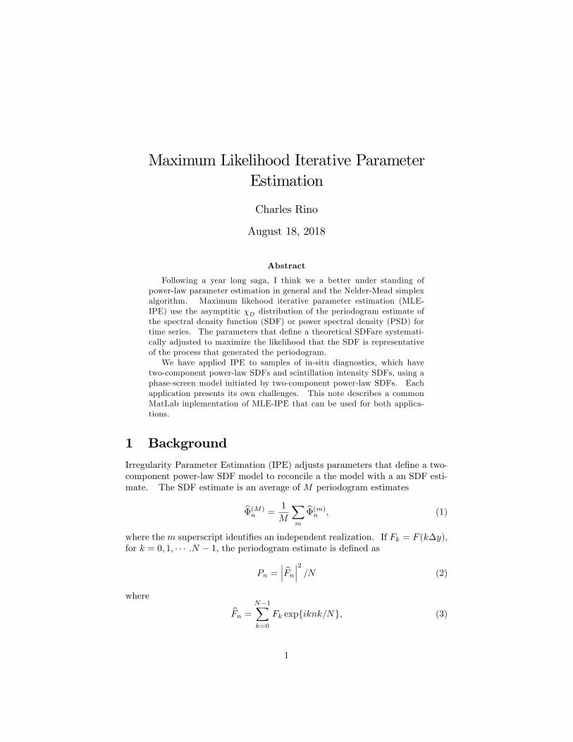
Parameter estimation for two-component power-law processes, include MLE,has been reviewed in the paper [2]. An intrinsic coupling between the tur-bulent strength and the low-frequency power-law index has been thoroughlyinvestigated. It was found that an MLE procedure with CsdB = 10 log10(Cs)is substituted for Cs gives better convergence and an smaller parameter errors.Figure 1 summarizes the MLE-IPE estimates with M = 1 for 1000 realizations.Each MLE-IPE search was initiated with a log-linear least-squares estimate ap-plied separately to large and small scale frequency ranges. Although the Csparameter has a larger spread, the average is correct, Cs = 10. Figure 2 showsthe exponential distribution that produces the average. Figure 3 shows scatterdiagrams of the spectral index and turbulent strength parameters. While the�1-Cs correlation is prominent in the scatter diagram it is not discernible in theerror summaries.

2.2 MLE IPE for Intensity Spectra

To explore the IPE rami�cations for intensity scintillation diagnostics, the Nerealizations were used to generate phase screens. The de�ning parameters for

3

Figure 1: Figure 11 from [2].

Figure 2: Figure 12 from [2].

4

Figure 3: Figure 13 from [2].

the phase screen are Cp, p1, p2, and q0. From [3], the relation between Cp andCs is

Cp = (2�K=f)2 [lCs] ; (11)

the path length, l, is absorbed in the de�nition of Cs. The remaining parametersconvert total electron content to phase:

K = rec=(2�)� 1016; (12)

where re is the classical electron radius, and c is the velocity of light.The intensity SDF from the phase screen theory depends on parameters

normalized to the Fresnel scale:

U = Cpp

�1 for �0 > 1�p2�p10 for �0 < 1

(13)

where k = 2�f=c, and

�F =px=k (14)

�0 = q0�F (15)

Cpp = Cp�p1�1F (16)

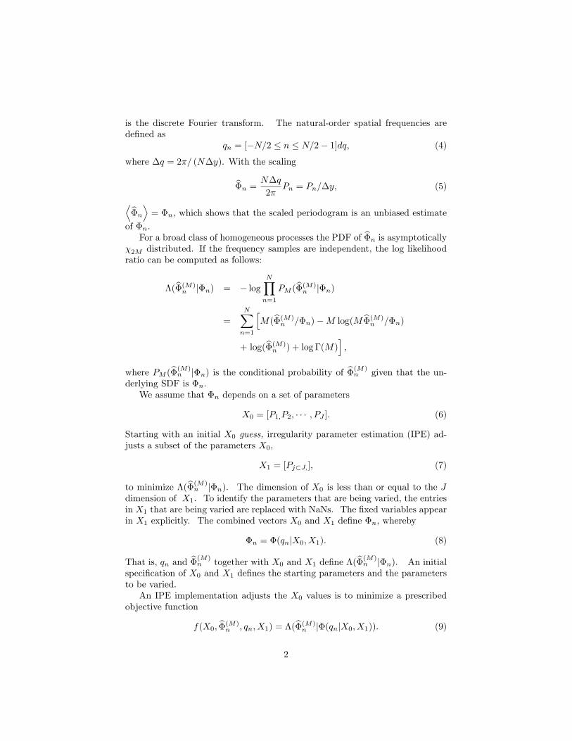
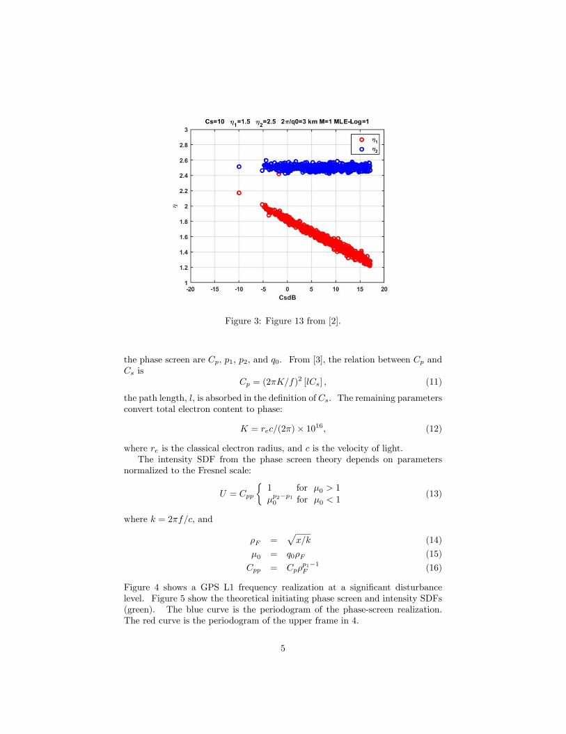
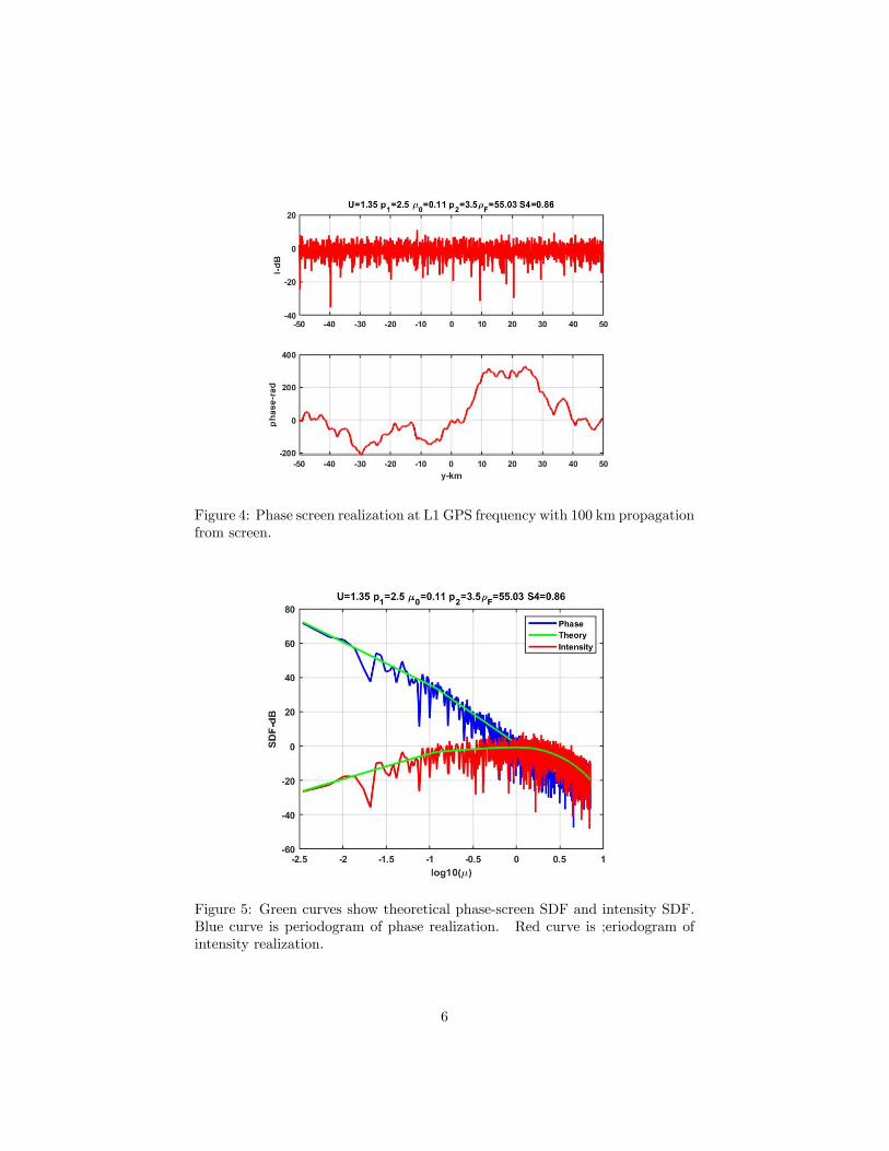
Figure 4 shows a GPS L1 frequency realization at a signi�cant disturbancelevel. Figure 5 show the theoretical initiating phase screen and intensity SDFs(green). The blue curve is the periodogram of the phase-screen realization.The red curve is the periodogram of the upper frame in 4.

5

Figure 4: Phase screen realization at L1 GPS frequency with 100 km propagationfrom screen.

Figure 5: Green curves show theoretical phase-screen SDF and intensity SDF.Blue curve is periodogram of phase realization. Red curve is ;eriodogram ofintensity realization.

6

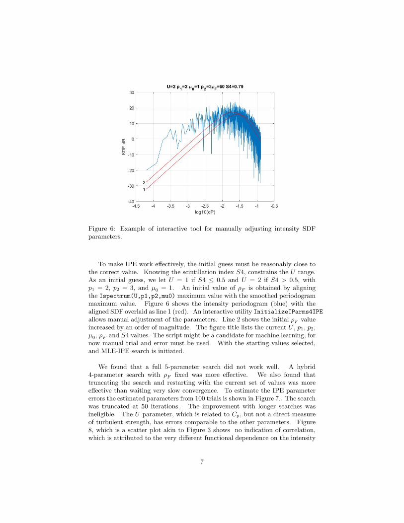
Figure 6: Example of interactive tool for manually adjusting intensity SDFparameters.

To make IPE work e¤ectively, the initial guess must be reasonably close tothe correct value. Knowing the scintillation index S4, constrains the U range.As an initial guess, we let U = 1 if S4 � 0:5 and U = 2 if S4 > 0:5, withp1 = 2, p2 = 3, and �0 = 1. An initial value of �F is obtained by aligningthe Ispectrum(U,p1,p2,mu0) maximum value with the smoothed periodogrammaximum value. Figure 6 shows the intensity periodogram (blue) with thealigned SDF overlaid as line 1 (red). An interactive utility InitializeIParms4IPEallows manual adjustment of the parameters. Line 2 shows the initial �F valueincreased by an order of magnitude. The �gure title lists the current U , p1, p2,�0, �F and S4 values. The script might be a candidate for machine learning, fornow manual trial and error must be used. With the starting values selected,and MLE-IPE search is initiated.

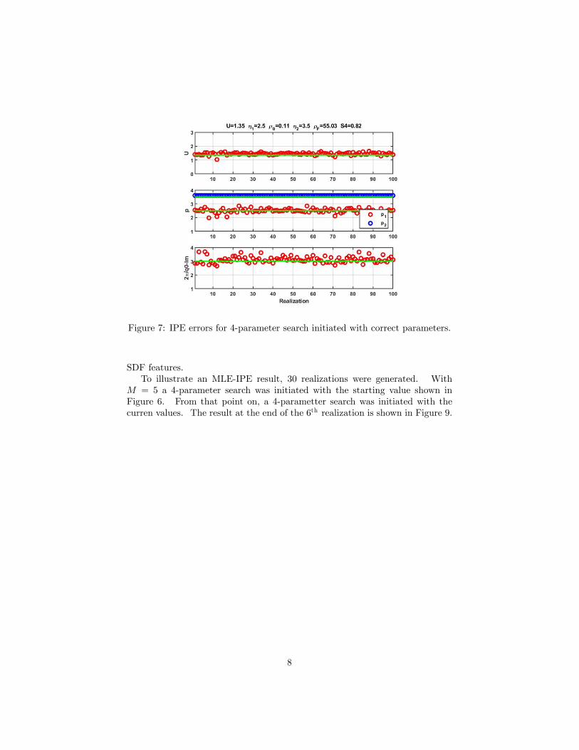
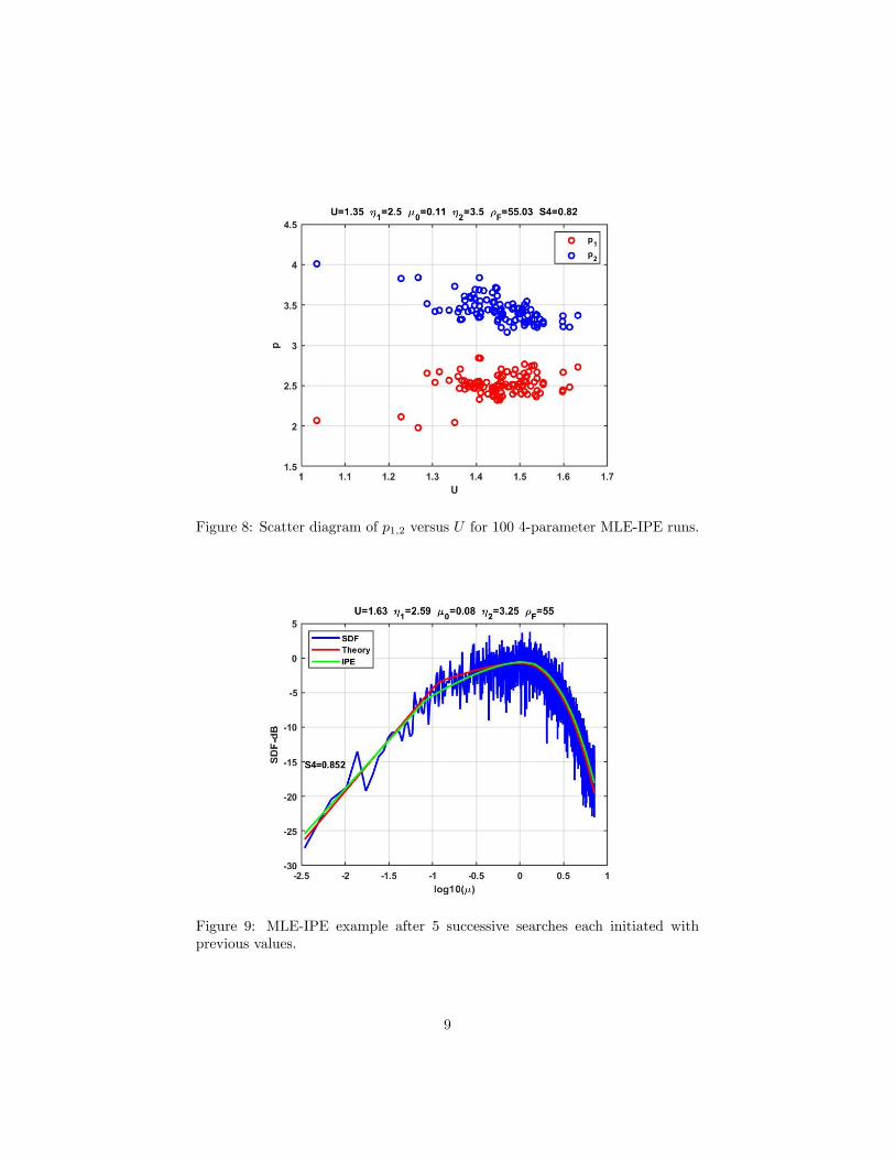
We found that a full 5-parameter search did not work well. A hybrid4-parameter search with �F �xed was more e¤ective. We also found thattruncating the search and restarting with the current set of values was moree¤ective than waiting very slow convergence. To estimate the IPE parametererrors the estimated parameters from 100 trials is shown in Figure 7. The searchwas truncated at 50 iterations. The improvement with longer searches wasineligible. The U parameter, which is related to Cp, but not a direct measureof turbulent strength, has errors comparable to the other parameters. Figure8, which is a scatter plot akin to Figure 3 shows no indication of correlation,which is attributed to the very di¤erent functional dependence on the intensity

7

Figure 7: IPE errors for 4-parameter search initiated with correct parameters.

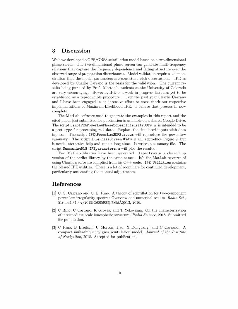
SDF features.To illustrate an MLE-IPE result, 30 realizations were generated. With

M = 5 a 4-parameter search was initiated with the starting value shown inFigure 6. From that point on, a 4-parametter search was initiated with thecurren values. The result at the end of the 6th realization is shown in Figure 9.

8

Figure 8: Scatter diagram of p1;2 versus U for 100 4-parameter MLE-IPE runs.

Figure 9: MLE-IPE example after 5 successive searches each initiated withprevious values.

9

3 Discussion

We have developed a GPS/GNSS scintillation model based on a two-dimensionalphase screen. The two-dimensional phase screen can generate multi-frequencyrelations that capture the frequency dependence and fading structure over theobserved range of propagation disturbances. Model validation requires a demon-stration that the model parameters are consistent with observations. IPE asdeveloped by Charlie Carrano is the basis for the validation. The current re-sults being pursued by Prof. Morton�s students at the University of Coloradoare very encouraging. However, IPE is a work in progress that has yet to beestablished as a reproducible procedure. Over the past year Charlie Carranoand I have been engaged in an intensive e¤ort to cross check our respectiveimplementations of Maximum-Likelihood IPE. I believe that process in nowcomplete.The MatLab software used to generate the examples in this report and the

cited paper just submitted for publication is available on a shared Google Drive.The script DemoIPE4PowerLawPhaseScreenIntensitySDFs.m is intended to bea prototype for processing real data. Replace the simulated inputs with datainputs. The script IPE4PowerLawSDFStats.m will reproduce the power-lawsummary. The script IPE4PhaseScreenStats.m will reproduce Figure 9, butit needs interactive help and runs a long time. It writes a summary �le. Thescript SummarizeMLE_IPEparameters.m will plot the results.Two MatLab libraries have been generated. Ispectrum is a cleaned up

version of the earlier library by the same names. It�s the MatLab resource ofusing Charlie�s software complied from his C++ code. IPE_Utilities containsthe blessed IPE utilities. There is a lot of room here for continued development,particularly automating the manual adjustments.

References

[1] C. S. Carrano and C. L. Rino. A theory of scintillation for two-componentpower law irregularity spectra: Overview and numerical results. Radio Sci.,51(doi:10.1002/2015RS005903):789â¼AS813, 2016.

[2] C Rino, C Carrano, K Groves, and T Yokoyama. On the characterizationof intermediate scale ionospheric structure. Radio Science, 2018. Submittedfor publication.

[3] C Rino, B Breitsch, U Morton, Jiao, X Dongyang, and C Carrano. Acompact multi-frequency gnss scintillation model. Journal of the Instituteof Navigation, 2018. Accepted for publication.

10