23
MAXIMUM MARGIN BAYIS NETWORK CLASSIFIERS ( Franz Pernkopf, Michael Wohlmayr, Sebastian Tschiatschek) Presented by: Silvi Mallavarapu
| Date post: | 13-Dec-2015 |
| Category: |
Documents |
| Upload: | evelyn-sutton |
| View: | 226 times |
| Download: | 2 times |

MAXIMUM MARGIN BAYIS NETWORK CLASSIFIERS
( Franz Pernkopf, Michael Wohlmayr, Sebastian Tschiatschek)
Presented by: Silvi Mallavarapu

CONTENTS: History
Parameterized Learning Methods
Structural Learning Methods
Experimental Results
Conclusion

HISTORY
Bayesian Probability was named after Thomas Bayes(1702-1761).The model is principled by determining probabilities of the outcomes.
In machine learning, naive Bayes classifiers are a family of simple probabilistic classifiers based on applying Bayes theorem with strong (naive) independence assumptions between the features.
Naive Bayes has been studied extensively since the 1950s. It was introduced under a different name into the text retrieval community in the early 1960s has remained a popular (baseline) method for text categorization.

Generative ML parameter learning The method of maximum likelihood selects the set of values of the model parameters that
maximizes the likelihood function. This maximizes the "agreement" of the selected model with the observed data, and for discrete random variables it indeed maximizes the probability of the observed data under the resulting distribution
The log likelihood function of a fixed structure of B is
Maximizing LL(B/S) leads to the ML estimate of the parameters
using Lagrange multipliers to constrain the parameters to a valid normalized probability distribution

Discriminative CL-Parameter Learning: Conditional Likelihood(CL) In informal contexts, "likelihood" is often used as a synonym for
"probability." But in statistical usage, a distinction is made depending on the roles of the outcome or parameter. Probability is used when describing a function of the outcome given a fixed parameter value. For example, if a coin is flipped 10 times and it is a fair coin, what is the probability of it landing heads-up every time? Likelihood is used when describing a function of a parameter given an outcome.
Maximizing CL is tightly connected to minimizing the empirical(proved by means if experimently) risk. Unfortunately, CL does not decompose as ML does. Consequently, there is no closed-form solution. The conditional log likelihood (CLL) is
A conjugate gradient algorithm or the EBW method have been proposed for maximizing CLL(B/S). For the sake of completeness, we briefly sketch the CG algorithm for CL optimization

Maximum Margin & Conjugate Gradient Method:
Usually, the maximum margin approach maximizes the margin of the sample with the smallest margin for a separable classification problem.
For a non-separable problem, we aim to relax this by introducing a soft margin, we focus on samples with For this purpose, we consider the hinge loss function and smooth hinge function
CG
It is an algorithm to find numerical solutions of a particular linear equations of symmetric and positive definite.
We use a conjugate gradient algorithm with line-search which requires both the objective function and its derivative.


NAIVE BAYES CLASSIFIERS Abstractly, naive Bayes is a conditional probability model: given a problem instance to
be classified, represented by a vector representing some n features (independent variables), it assigns to this instance probabilities for each of k possible outcomes or classes.
The problem with the above formulation is that if the number of features n is large or if a feature can take on a large number of values, then basing such a model on probability tables is infeasible. We therefore reformulate the model to make it more tractable. Using Bayes' theorem, the conditional probability can be decomposed as
In plain English, using Bayesian probability terminology, the above equation can be written as

Naive Bayes Structure:As we know these are independent with each other and doesn't depend on other attributes these do not have any structure but basic structure given by:
C
x1 x2 x3

TAN-CMI The conditional mutual information (CMI) between the attributes given the class variable
is computed as:
where denotes the expectation of f(X) with respect to P(X). It measures the information between Xi and Xj in the context of C. In an algorithm for constructing TAN networks using this measure is provided.
We briefly review this algorithm in the following:
1. Compute the pairwise CMI for all 1≤ i ≤ N and i ≤ j≤ N
2.Build an un-directed 1-tree using MST.
3.Now transform undirected tree to directed tree.

TAN-CMI structure: Initially a NBC structure is considered and then dependence occurs showing more realistic.
Here it depends on Variable C along with one more dependent(x).
c
x1 x2 x3

Greedy Discriminate Structure Learning(TAN-CR) This method proceeds as follows: A network is initialized to NB and at each iteration an edge is added
that gives the largest improvement of the scoring function while maintaining a partial 1-tree.
The process of adding edges is terminated when there is no edge which further improves the score.
Thus, it might result in a partial 1-tree (forest) over the attributes. This approach is computationally expensive since, each time an edge is added, the scores for all O(N^2) edges need to be reevaluated due to the discriminative non decomposable scoring functions we employ. Overall, for learning a k-tree structure, O(N^k+2) score evaluations are necessary.
It has small error rate.
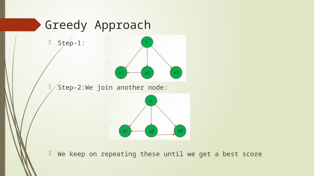
Greedy Approach Step-1:
Step-2:We join another node:
We keep on repeating these until we get a best score

Note: Since we follow a tree structure in all methods remember that any node will not have two
parents excluding C. That means x1 can dependent on x2,c not more that:
These type of structure does not exist and it is a wrong assumption.
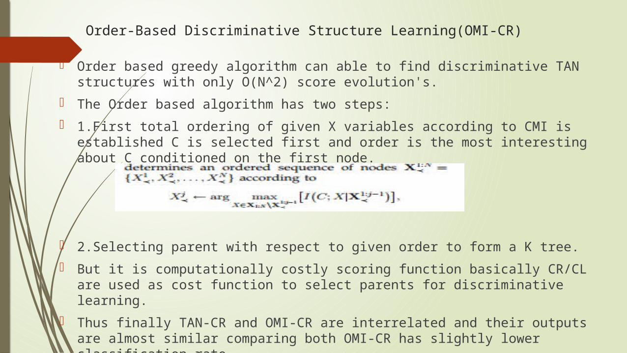
Order-Based Discriminative Structure Learning(OMI-CR)
Order based greedy algorithm can able to find discriminative TAN structures with only O(N^2) score evolution's.
The Order based algorithm has two steps:
1.First total ordering of given X variables according to CMI is established C is selected first and order is the most interesting about C conditioned on the first node.
2.Selecting parent with respect to given order to form a K tree.
But it is computationally costly scoring function basically CR/CL are used as cost function to select parents for discriminative learning.
Thus finally TAN-CR and OMI-CR are interrelated and their outputs are almost similar comparing both OMI-CR has slightly lower classification rate.

Experimental Results & Their Compression: Here we consider Three different type of data TIMIT-4/6 data is extracted from TIMIT
speech corpus and for Hand written digital recognition using MNIST,USPS Data these results are seen in comparison to classifiers with respect to parameter learning with standard deviation.


Missing Features Vs Classification Performance: In Structural learning Method:
Different structural learning Methods with generative parameterization.
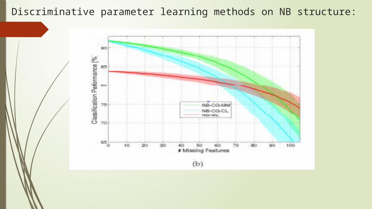
Discriminative parameter learning methods on NB structure:

Example considering Nature/Spectrum As ground reference a classification performed at Purdue University was used containing seven
classes, namely roof, road, grass, trees, trail, water, and shadow.10 The aerial image using bands 63, 52, and 36 for red, green, and blue colors, respectively and the reference image are shown in Figs.
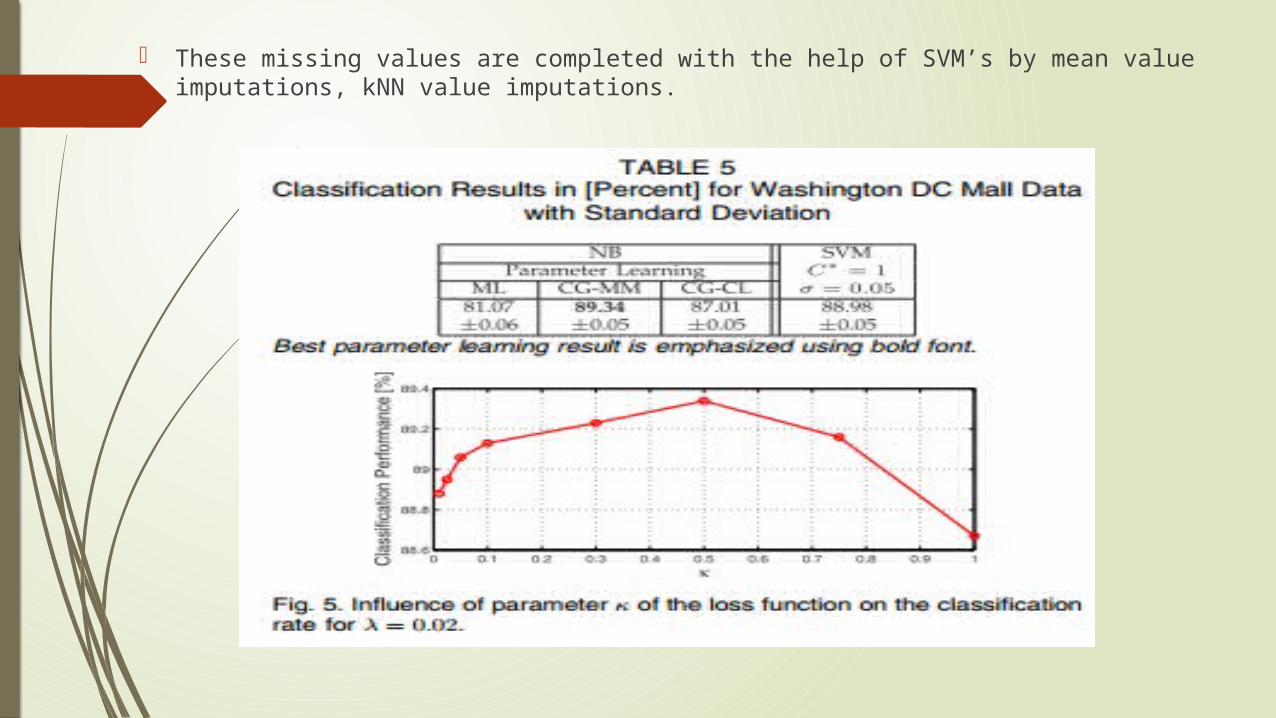
These missing values are completed with the help of SVM’s by mean value imputations, kNN value imputations.

Conclusion: Here we studied of with Parameter learning algorithms for Bayesian network classifiers
based on maximizing the margin. For margin optimization we introduced a conjugate gradient algorithm.
We also studied structural algorithm TAN-CMI,TAN-CR,TAN-OMI CR
The Bayesian network classifiers require fewer parameters than the SVM and can directly deal with missing features, a case where discriminative classifiers usually require imputation techniques.

References: E. Keogh and M. Pazzani, “Learning Augmented Bayesian Classifiers: A Comparison of
Distribution-Based and Classification-Based Approaches,” Proc. Workshop Artificial Intelligence and Statistics, pp. 225-230, 1999.
F. Pernkopf, “Bayesian Network Classifiers versus Selective k-NN Classifier,” Pattern Recognition, vol. 38, no. 3, pp. 1-10, 2005.
F. Pernkopf and J. Bilmes, “Order-Based Discriminative Structure Learning for Bayesian Network Classifiers,” Proc. Int’l Symp. Artificial Intelligence and Math., 2008.
Y. LeCun, L. Bottou, Y. Bengio, and P. Haffner, “Gradient-Based Learning Applied to Document Recognition,” Proc. IEEE, vol. 86,no. 11, pp. 2278-2324, Nov. 1998.
C. Bishop, Neural Networks for Pattern Recognition. Oxford Univ.Press, 1995.


![Atlas of Topog., Appl. Human Anat. [Vol. 1 Head and Neck] - E. Pernkopf (Lippinkott) WW](https://static.documents.pub/doc/80x56/613cab489cc893456e1e9998/atlas-of-topog-appl-human-anat-vol-1-head-and-neck-e-pernkopf-lippinkott.jpg)


![arXiv:1310.5953v2 [hep-ph] 18 Mar 2014 · Mark G. Alford, 1,S. Kumar Mallavarapu, yAndreas Schmitt,2, zand Stephan Stetina2, x 1Department of Physics, Washington University St Louis,](https://static.documents.pub/doc/80x56/5b54f1e57f8b9add3a8db212/arxiv13105953v2-hep-ph-18-mar-2014-mark-g-alford-1s-kumar-mallavarapu.jpg)


![Excitations in relativistic superfluids - Menunpcsm/slides/2nd/Stetina.pdf · [M.G. Alford, S. K. Mallavarapu, A. Schmitt, S. Stetina, PRD87, 065001 (2013)] Stephan Stetina Institute](https://static.documents.pub/doc/80x56/5afa2f6d7f8b9a44658ebc94/excitations-in-relativistic-superfluids-npcsmslides2ndstetinapdfmg-alford.jpg)
