Maximum-principle-satisfying and positivity-preserving high … · 2014-02-14 ·...

Maximum-principle-satisfying and

positivity-preserving high order schemes

for conservation laws: Survey and new

developments

By Xiangxiong Zhang1 and Chi-Wang Shu2 †1Department of Mathematics, Brown University, Providence, RI 02912, USA.

2Division of Applied Mathematics, Brown University, Providence, RI 02912, USA.

In Zhang & Shu (2010b), genuinely high order accurate finite volume and discontin-uous Galerkin schemes satisfying a strict maximum principle for scalar conservationlaws were developed. The main advantages of such schemes are their provable highorder accuracy and their easiness for generalization to multi-dimensions for arbi-trarily high order schemes on structured and unstructured meshes. The same ideacan be used to construct high order schemes preserving the positivity of certainphysical quantities, such as density and pressure for compressible Euler equations,water height for shallow water equations, and density for Vlasov-Boltzmann trans-port equations. These schemes have been applied in computational fluid dynamics,computational astronomy and astrophysics, plasma simulation, population mod-els and traffic flow models. In this paper, we first review the main ideas of thesemaximum-principle-satisfying and positivity-preserving high order schemes, thenpresent a simpler implementation which will result in a significant reduction ofcomputational cost especially for weighted essentially nonoscillatory (WENO) fi-nite volume schemes.

Keywords: hyperbolic conservation laws; discontinuous Galerkin method;

weighted essentially non-oscillatory finite volume scheme;

positivity-preserving; maximum-principle-satisfying; high order accuracy

1. Introduction

An important property of the unique entropy solution to the scalar conservationlaw

ut + ∇ · F(u) = 0, u(x, 0) = u0(x) (1.1)

is that it satisfies a strict maximum principle, namely, if M = maxx u0(x), m =minx u0(x), then u(x, t) ∈ [m,M ] for any x and t. This property is also natu-rally desired for numerical schemes solving (1.1) since numerical solutions outsideof [m,M ] often are meaningless physically, such as negative density, or negativepercentage or percentage larger than one for a component in a multi-componentmixture.

One of the main difficulties in solving (1.1) is that the solution may containdiscontinuities even if the initial condition is smooth. Moreover, the weak solutions

† Author for correspondence ([email protected]).

Article submitted to Royal Society TEX Paper

2 X. Zhang and C.-W. Shu

of (1.1) may not be unique. Therefore, the nonlinear stability and convergenceto the unique entropy solution must be considered for the numerical schemes.Total-variation (TV) stable functions form a compact space, so a conservativeTV-stable scheme will produce a subsequence converging to a weak solution bythe Lax-Wendroff Theorem. The E-schemes including Godunov, Lax-Friedrichsand Engquist-Osher methods satisfy an entropy inequality and are total-variation-diminishing (TVD) thus maximum-principle-satisfying. However, E-schemes are atmost first order accurate. In fact, any TVD scheme in the sense of measuring thevariation of grid point values or cell averages will be at most first order accuratearound smooth extrema, see Osher & Chakravarthy (1984), although TVD schemescan be designed for any formal order of accuracy for smooth monotone solutions,e.g., the high resolution schemes.

For conventional maximum-principle-satisfying finite difference schemes, the so-lution is at most second order accurate, for instance, only the second order centralscheme was proved to satisfy the maximum principle in Jiang & Tadmor (1998).This fact has a simple proof due to Ami Harten. For simplicity we consider a finitedifference scheme, namely unj is the numerical solution approximating the pointvalues u(xj , t

n) of the exact solution, where n is the time step and j denotes thespatial grid index. Assume the scheme satisfies the maximum principle

maxjun+1j ≤ max

junj . (1.2)

Consider the linear convection equation ut + ux = 0, u(x, 0) = sin(2πx), x ∈ [0, 1]with periodic boundary conditions. Set the grid as xj = (j − 1

2 )∆x where ∆x = 1N

and N is a multiple of 4. The numerical initial value is u0j = sin(2πxj). Without

loss of generality, assume ∆t = 12∆x. At the grid point j = N

4 + 1 and t = ∆t,

the exact solution is sin(2π(xj − ∆t)) = sin(2π((N4 + 12 )∆x − ∆t)) = sin(π2 ) = 1

and the numerical solution is u1j ≤ max

ju0j = sin(π2 − π

N ) by (1.2). The error of

the scheme at the grid point j = N4 + 1 after one time step is equal to |1 − u1

j | =

1 − u1j ≥ 1 − sin(π2 − π

N ) = π2

2 ∆x2 + O(∆x3). That is, even after one time stepthe scheme is already at most second order accurate. A similar proof also works forfinite volume schemes where the numerical solution approximates cell averages ofthe exact solution.

The simple derivation above implies that (1.2) is too restrictive for the schemeto be higher than second order accurate. A heuristic point of view to understandthe restriction is, some high order information of the exact solution is lost since weonly measure the total variation or the maximum at the grid points or in cell aver-ages. To overcome this difficulty, Sanders proposed to measure the total variationof the reconstructed polynomials and he succeeded in designing a third order TVDscheme for one-dimensional scalar conservation laws in Sanders (1988), which hasbeen extended to higher order in Zhang & Shu (2010a). But it is very difficultto generalize Sanders’ scheme to higher space dimension. By measuring the max-imum of the reconstructed polynomial, Liu and Osher constructed a third ordernon-oscillatory scheme in Liu & Osher (1996), which could be generalized to twospace dimensions. However, it could be proven maximum-principle-satisfying onlyfor the linear equation. The key step of maximum-principle-satisfying high orderschemes above is a high order accurate time evolution which preserves the max-

Article submitted to Royal Society

Maximum-principle-satisfying and positivity-preserving schemes 3

imum principle. The exact time evolution satisfies this property and it was usedin Sanders (1988), Zhang & Shu (2010a), Liu & Osher (1996). Unfortunately,it is very difficult, if not impossible, to implement such exact time evolution formulti-dimensional nonlinear scalar equations or systems of conservation laws.

Successful high order numerical schemes for hyperbolic conservation laws in-clude, among others, the Runge-Kutta discontinuous Galerkin (RKDG) methodwith a total variation bounded (TVB) limiter, e.g. in Cockburn & Shu (1989), theessentially non-oscillatory (ENO) finite volume and finite difference schemes, e.g. inHarten et al. (1987), Shu & Osher (1988), and the weighted ENO (WENO) finitevolume and finite difference schemes, e.g. in Liu et al. (1994), Jiang & Shu (1996).Although these schemes are nonlinearly stable in numerical experiments and someof them can be proven to be total variation stable, they do not in general satisfy astrict maximum principle. In Zhang & Shu (2010b), we proved a sufficient condi-tion for the cell averages of the numerical solutions in a high order finite volume ora discontinuous Galerkin (DG) scheme with the strong stability preserving (SSP)time discretization, e.g., Shu & Osher (1988), Shu (1988), to be bounded in [m,M ]for (1.1). We have also proved that this sufficient condition can be enforced by asimple scaling limiter introduced in Liu & Osher (1996) without destroying accu-racy for smooth solutions. In other words, we have constructed a high order schemeby adding a simple limiter to a finite volume WENO/ENO or RKDG scheme andit can be proven to be high order accurate and maximum-principle-satisfying. Thiswas the first time that genuinely high order schemes are obtained satisfying a strictmaximum principle especially for multidimensional nonlinear problems.

For hyperbolic conservation law systems, the entropy solutions in general do notsatisfy the maximum principle. We consider the positivity of some important quan-tities instead. For instance, density and pressure in compressible Euler equations,and water height in shallow water equations should be nonnegative physically. Inpractice, failure of preserving positivity of such quantities causes blow-ups of thecomputation because the linearized system will have imaginary eigenvalues thusthe initial value problems will be ill-posed. From the point of view of stability, it ishighly desired to design schemes which can be proven to be positivity-preserving.Most commonly used high order numerical schemes for solving hyperbolic con-servation law systems do not in general satisfy such properties automatically. Itis very difficult to design a conservative high order accurate scheme preservingthe positivity. In Zhang & Shu (2010c, 2011) and Zhang et al. (2011), we havegeneralized the maximum-principle-satisfying techniques to construct conservativepositivity-preserving high order finite volume and DG schemes for compressible Eu-ler equations, which could be regarded as an extension of the positivity-preservingschemes in Perthame & Shu (1996).

In this paper, we first review the general framework to construct maximum-principle-satisfying and positivity-preserving schemes of arbitrarily high order ac-curacy. In §2, we illustrate the main ideas in the context of scalar conservationlaws. We then discuss generalizations of this idea to other equations and systemsin §3 and §4. In §5, we propose a more efficient implementation of the frameworkfor WENO finite volume schemes, and provide numerical examples to demonstratetheir performance. Concluding remarks are given in §6.



2. Maximum-principle-satisfying high order schemes for

scalar conservation laws

(a) One-dimensional scalar conservation laws

We consider the one-dimensional version of (1.1) in this section:

ut + f(u)x = 0, u(x, 0) = u0(x). (2.1)

(i) The first order schemes

It is well known that a first order monotone scheme solving (2.1) satisfies thestrict maximum principle. A first order monotone scheme has the form

un+1j = unj − λ[f(unj , u

nj+1) − f(unj−1, u

nj )] ≡ Hλ(u

nj−1, u

nj , u

nj+1), (2.2)

where λ = ∆t∆x with ∆t and ∆x being the temporal and spatial mesh sizes (we

assume uniform mesh size for the structured mesh cases in this paper for simplicityin presentation, however the methodology does not have a uniform or smooth meshrestriction), and f(a, b) is a monotone flux, namely it is Lipschitz continuous in botharguments, non-decreasing (henceforth referred to as increasing with a slight abuseof the terminology) in the first argument and non-increasing (henceforth referred

to as decreasing) in the second argument, and consistent f(a, a) = f(a). Undersuitable CFL conditions, typically of the form

αλ ≤ 1, α = max |f ′(u)|, (2.3)

for e.g. Lax-Friedrichs scheme and Godunov scheme, one can prove that the functionHλ(a, b, c) are increasing in all three arguments, and consistency impliesHλ(a, a, a) =a. We therefore immediately have the strict maximum principle

m = Hλ(m,m,m) ≤ un+1j = Hλ(u

nj−1, u

nj , u

nj+1) ≤ Hλ(M,M,M) = M

provided m ≤ unj−1, unj , u

nj+1 ≤M .

(ii) High order spatial discretization

Now consider high order finite volume or DG methods, for example, the WENOfinite volume method in Liu et al. (1994) and the DG method in Cockburn & Shu(1989) solving (2.1). We only discuss the Euler forward temporal discretizationin this subsection and leave higher order temporal discretization to §2 a (iv). Thefinite volume method or the scheme satisfied by the cell averages in the DG methoddiscretization can be written as:

un+1j = unj − λ[f(u−

j+ 12

, u+j+ 1

2

) − f(u−j− 1

2

, u+j− 1

2

)] ≡ Gλ(unj , u

−j+ 1

2

, u+j+ 1

2

, u−j− 1

2

, u+j− 1

2

),

(2.4)where unj is the approximation to the cell averages of u(x, t) in the cell Ij =

[xj− 12, xj+ 1

2] at time level n, and u−

j+ 12

, u+j+ 1

2

are the high order approximations

of the nodal values u(xj+ 12, tn) within the cells Ij and Ij+1 respectively, and f(·, ·)

is again a monotone flux. These values are either reconstructed from the cell aver-ages unj in a finite volume method or read directly from the evolved polynomials in



a DG method. We assume that there is a polynomial pj(x) (either reconstructed ina finite volume method or evolved in a DG method) with degree k, where k ≥ 1,defined on Ij such that unj is the cell average of pj(x) on Ij , u

+j− 1

2

= pj(xj− 12) and

u−j+ 1

2

= pj(xj+ 12).

Given a scheme in the form of (2.4), assuming unj ∈ [m,M ] for all j, we would

like to derive some sufficient conditions to ensure un+1j ∈ [m,M ]. A very natural

first attempt is to see if there is a restriction on λ such that, if all five argumentsof G are in [m,M ]

m ≤ unj , u−j+ 1

2

, u+j+ 1

2

, u−j− 1

2

, u+j− 1

2

≤M,

then we could prove un+1j ∈ [m,M ]. Unfortunately, one can easily build counter

examples to show that this cannot be always true. The problem is that the functionGλ(a, b, c, d, e) in (2.4) is only monotonically increasing in the first, third and fourtharguments and is monotonically decreasing in the other two arguments. Hence thestrategy to prove maximum principle for first order monotone schemes cannot berepeated here. In the literature, many attempts have been made to further limitthe four arguments u−

j+ 12

, u+j+ 1

2

, u−j− 1

2

, u+j− 1

2

(remember the cell average unj cannot

be changed due to conservation) in the arguments of Gλ in (2.4) to guarantee thatun+1j ∈ [m,M ]. However, these limiters always kill accuracy near smooth extrema.

Our approach follows a different strategy. We consider an N -point LegendreGauss-Lobatto quadrature rule on the interval Ij = [xj− 1

2, xj+ 1

2], which is exact

for the integral of polynomials of degree up to 2N − 3. We denote these quadraturepoints on Ij as

Sj = {xj− 12

= x1j , x

2j , · · · , x

N−1j , xNj = xj+ 1

2}. (2.5)

Let wα be the quadrature weights for the interval [− 12 ,

12 ] such that

N∑α=1

wα = 1.

Choose N to be the smallest integer satisfying 2N − 3 ≥ k, then

unj =1

∆x

∫

Ij

pj(x)dx =

N∑

α=1

wαpj(xαj ) =

N−1∑

α=2

wαpj(xαj )+w1u

+j− 1

2

+wNu−j+ 1

2

. (2.6)

We then have the following theorem. We assume that the monotone flux f corre-sponds to a monotone scheme (2.2) under the CFL condition (2.3).

Theorem 2.1. Consider a finite volume scheme or the scheme satisfied by the cellaverages of the DG method (2.4), associated with the approximation polynomialspj(x) of degree k (either reconstruction or DG polynomials) in the sense that unj =1

∆x

∫Ijpj(x)dx, u

+j− 1

2

= pj(xj− 12) and u−

j+ 12

= pj(xj+ 12). If u−

j− 12

, u+j+ 1

2

and pj(xαj )

(α = 1, · · · , N) are all in the range [m,M ], then un+1j ∈ [m,M ] under the CFL

conditionλa ≤ w1. (2.7)

Proof. With (2.6), by adding and subtracting f(u+j− 1

2

, u−j+ 1

2

), the scheme (2.4) can

be rewritten as

un+1j =

N−1∑

α=2

wαpj(xαj ) + wN

(u−j+ 1

2

−λ

wN

[f

(u−j+ 1

2

, u+j+ 1

2

)− f

(u+j− 1

2

, u−j+ 1

2

)])



+w1

(u+j− 1

2

−λ

w1

[f

(u+j− 1

2

, u−j+ 1

2

)− f

(u−j− 1

2

, u+j− 1

2

)])

=

N−1∑

α=2

wαpj(xαj ) + wNHλ/bωN

(u+j− 1

2

, u−j+ 1

2

, u+j+ 1

2

) + w1Hλ/bω1(u−j− 1

2

, u+j− 1

2

, u−j+ 1

2

).

(2.8)

Noticing that w1 = wN and Hλ/bω1is monotone under the CFL condition (2.7),

we can see from (2.8) that un+1j is a monotonically increasing function of all the

arguments involved, namely u−j− 1

2

, u+j+ 1

2

and pj(xαj ) for 1 ≤ j ≤ N . The same proof

for the first order monotone scheme now applies to imply un+1j ∈ [m,M ].

Remark We recall that the CFL condition for linear stability for the DG schemeusing polynomial of degree k is λa ≤ 1

2k+1 in Cockburn & Shu (1989), which isclose to the CFL condition (2.7).

(iii) The linear scaling limiter

Theorem 2.1 tells us that for the scheme (2.4), we need to modify pj(x) suchthat pj(x) ∈ [m,M ] for all x ∈ Sj where Sj is defined in (2.5). For all j, assumeunj ∈ [m,M ], we use the modified polynomial pj(x) by the limiter introduced in Liu& Osher (1996), i.e.,

pj(x) = θ(pj(x) − unj ) + unj , θ = min

{∣∣∣∣M − unjMj − unj

∣∣∣∣ ,∣∣∣∣m− unjmj − unj

∣∣∣∣ , 1}, (2.9)

withMj = max

x∈Ij

pj(x), mj = minx∈Ij

pj(x). (2.10)

Let u+j− 1

2

= pj(xj− 12) and u−

j+ 12

= pj(xj+ 12). We get the revised scheme of (2.4):

un+1j = unj − λ[f(u−

j+ 12

, u+j+ 1

2

) − f(u−j− 1

2

, u+j− 1

2

)]. (2.11)

The scheme (2.11) satisfies the sufficient condition in theorem 2.1. We will showin the next lemma that this limiter does not destroy the uniform high order ofaccuracy.

Lemma 2.2. Assume unj ∈ [m,M ], then (2.9)-(2.10) gives a (k + 1)-th orderaccurate limiter.

Proof. We need to show pj(x) − pj(x) = O(∆xk+1) for any x ∈ Ij . We only prove

the case that pj(x) is not a constant and θ =∣∣∣ M−un

j

Mj−unj

∣∣∣, the other cases being similar.

Since unj ≤M and unj ≤Mj , we have θ = (M − unj )/(Mj − unj ). Therefore,

pj(x) − pj(x) = θ(pj(x) − unj ) + unj − pj(x)

= (θ − 1)(pj(x) − unj )

=M −Mj

Mj − unj(pj(x) − unj )



= (M −Mj)pj(x) − unjMj − unj

.

By the definition of θ in (2.9), θ =∣∣∣ M−un

j

Mj−unj

∣∣∣ implies that θ =∣∣∣ M−un

j

Mj−unj

∣∣∣ < 1, i.e.

there is an overshoot Mj > M , and the overshoot Mj − M = O(∆xk+1) sincepj(x) is an approximation with error O(∆xk+1). Thus we only need to prove that∣∣∣pj(x)−u

nj

Mj−unj

∣∣∣ ≤ Ck, where Ck is a constant depending only on the polynomial degree k.

In Liu & Osher (1996), C2 = 3 is proved. We now prove the existence of Ck for anyk. Assume pj(x) = a0+a1(

x−xj

∆x )+ · · ·+ak(x−xj

∆x )k and p(x) = a0+a1x+ · · ·+akxk,

then the cell average of p(x) on I = [− 12 ,

12 ] is p = unj and max

x∈Ip(x) = Mj . So we

have

maxx∈Ij

∣∣∣∣pj(x) − unjMj − unj

∣∣∣∣ = maxx∈I

∣∣∣∣∣∣p(x) − p

maxy∈I

p(y) − p

∣∣∣∣∣∣.

Let q(x) = p(x) − p, then it suffices to prove the existence of Ck such that

∣∣∣∣∣∣

minx∈I

p(x) − p

maxx∈I

p(x) − p

∣∣∣∣∣∣=

∣∣∣∣∣∣

minx∈I

q(x)

maxx∈I

q(x)

∣∣∣∣∣∣≤ Ck.

It is easy to check that |minx∈I

q(x)| and |maxx∈I

q(x)| are both norms on the finite

dimensional linear space consisting of all polynomials of degree k whose averageson the interval I are zero. Any two norms on this finite dimensional space areequivalent, hence their ratio is bounded by a constant Ck.

Notice that in (2.10) we need to evaluate the maximum/minimum of a polyno-mial. We prefer to avoid evaluating the extrema of a polynomial, especially sincewe will extend the method to two dimensions. Since we only need to control thevalues at several points, we could replace (2.10) by

Mj = maxx∈Sj

pj(x), mj = minx∈Sj

pj(x), (2.12)

and the limiter (2.9) and (2.12) is sufficient to enforce pj(x) ∈ [m,M ], ∀x ∈ Sj . Asto the accuracy, (2.12) is a less restrictive limiter than (2.10), so the accuracy willnot be destroyed. Also, it is a conservative limiter because the it does not changethe cell average of the polynomial.

For the conservative maximum-principle-satisfying scheme (2.11), it is straight-forward to prove the following stability result:

Theorem 2.3. Assuming periodic or zero boundary conditions, then the numericalsolution of (2.11) satisfies

∑

j

|un+1j −m| =

∑

j

|unj −m|,∑

j

|un+1j −M | =

∑

j

|unj −M |.

Proof. Taking the sum of (2.11) over j, we obtain∑j u

n+1j =

∑j u

nj . Since the

numerical solutions are maximum-principle-satisfying, namely, un+1j , unj ∈ [m,M ],



we have∑

j

|un+1 −m| =∑

j

(un+1 −m) =∑

j

(un −m) =∑

j

|un −m|.

The other equality follows similarly.

Remark As an easy corollary, if the solution is non-negative, namely if m ≥ 0,then we have the L1 stability

∑j |u

n+1j | =

∑j |u

nj |.

(iv) High order temporal discretization

We use strong stability preserving (SSP) high order time discretizations. Formore details, see Shu & Osher (1988), Shu (1988). For example, the third orderSSP Runge-Kutta method in Shu & Osher (1988) (with the CFL coefficient c = 1)is

u(1) = un + ∆tF (un)

u(2) =3

4un +

1

4(u(1) + ∆tF (u(1))

un+1 =1

3un +

2

3(u(2) + ∆tF (u(2)))

where F (u) is the spatial operator, and the third order SSP multi-step method inShu (1988) (with the CFL coefficient c = 1

3 ) is

un+1 =16

27(un + 3∆tF (un)) +

11

27(un−3 +

12

11∆tF (un−3)).

Here, the CFL coefficient c for a SSP time discretization refers to the fact that, ifwe assume the Euler forward time discretization for solving the equation ut = F (u)is stable in a norm or a semi-norm under a time step restriction ∆t ≤ ∆t0, then thehigh order SSP time discretization is also stable in the same norm or semi-normunder the time step restriction ∆t ≤ c∆t0.

Since a SSP high order time discretization is a convex combinations of Eulerforward, the full scheme with a high order SSP time discretization will still satisfythe maximum principle. The limiter (2.9) and (2.12) should be used for each stagein a Runge-Kutta method or each step in a multi-step method. For details of theimplementation, see Zhang & Shu (2010b).

(b) Two-dimensional extensions

Consider the two-dimensional scalar conservation laws ut + f(u)x + g(u)y =0, u(x, y, 0) = u0(x, y) with M = max

x,yu0(x, y),m = min

x,yu0(x, y). We only discuss

the DG method with the Euler forward time discretization in this section, but allthe results also hold for the finite volume scheme (e.g. ENO and WENO).

(i) Rectangular meshes

For simplicity we assume we have a uniform rectangular mesh. At time level n,we have an approximation polynomial pij(x, y) of degree k with the cell average



unij on the (i, j) cell [xi− 12, xi+ 1

2]× [yj− 1

2, yj+ 1

2]. Let u+

i− 12,j(y), u−

i+ 12,j(y), u+

i,j− 12

(x),

u−i,j+ 1

2

(x) denote the traces of pij(x, y) on the four edges respectively. A finite

volume scheme or the scheme satisfied by the cell averages of a DG method on arectangular mesh can be written as

un+1ij = unij −

∆t

∆x∆y

∫ yj+ 1

2

yj− 1

2

f[u−i+ 1

2,j(y), u+

i+ 12,j(y)

]− f

[u−i− 1

2,j(y), u+

i− 12,j(y)

]dy

−∆t

∆x∆y

∫ xi+1

2

xi− 1

2

g[u−i,j+ 1

2

(x), u+i,j+ 1

2

(x)]− g

[u−i,j− 1

2

(x), u+i,j− 1

2

(x)]dx,

where f(·, ·), g(·, ·) are one dimensional monotone fluxes. The integrals can beapproximated by quadratures with sufficient accuracy. Let us assume that we usea Gauss quadrature with L points, which is exact for single variable polynomials ofdegree k. We assume Sxi = {xβi : β = 1, · · · , L} denote the Gauss quadrature points

on [xi− 12, xi+ 1

2], and Syj = {yβj : β = 1, · · · , L} denote the Gauss quadrature points

on [yj− 12, yj+ 1

2]. For instance, (xi− 1

2, yβj ) (β = 1, · · · , L) are the Gauss quadrature

points on the left edge of the (i, j) cell. The subscript β will denote the values at

the Gauss quadrature points, for instance, u+i− 1

2,β

= u+i− 1

2,j(yβj ). Also, wβ denotes

the corresponding quadrature weight on interval [− 12 ,

12 ], so that

∑Lβ=1 wβ = 1. We

will still need to use the Gauss-Lobatto quadrature rule, and we distinguish thetwo quadrature rules by adding hats to the Gauss-Lobatto points, i.e., Sxi = {xαi :α = 1, · · · , N} will denote the Gauss-Lobatto quadrature points on [xi− 1

2, xi+ 1

2],

and Syj = {yαj : α = 1, · · · , N} will denote the Gauss-Lobatto quadrature points on[yj− 1

2, yj+ 1

2]. Subscripts or superscripts β will be used only for Gauss quadrature

points and α only for Gauss-Lobatto points.Let λ1 = ∆t

∆x and λ2 = ∆t∆y , then the scheme becomes

un+1ij = unij − λ1

L∑

β=1

wβ

[f(u−

i+ 12,β, u+i+ 1

2,β

) − f(u−i− 1

2,β, u+i− 1

2,β

)]

−λ2

L∑

β=1

wβ

[g(u−

β,j+ 12

, u+β,j+ 1

2

) − g(u−β,j− 1

2

, u+β,j− 1

2

)]. (2.13)

We want to find a sufficient condition for the scheme (2.13) to satisfy un+1ij ∈

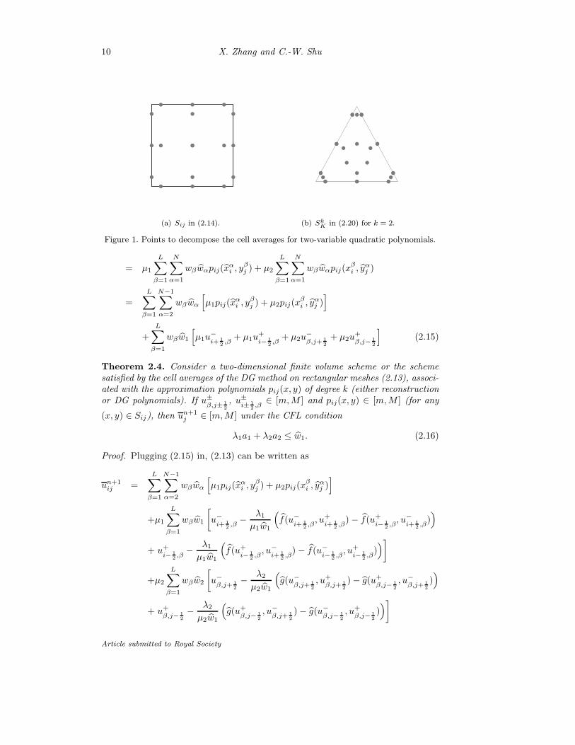
[m,M ]. We use ⊗ to denote the tensor product, for instance, Sxi ⊗ Syj = {(x, y) :x ∈ Sxi , y ∈ Syj }. Define the set Sij as

Sij = (Sxi ⊗ Syj ) ∪ (Sxi ⊗ Syj ). (2.14)

See figure 1(a) for an illustration for k = 2. For simplicity, let µ1 = λ1a1

λ1a1+λ2a2and

µ2 = λ2a2

λ1a1+λ2a2where a1 = max |f ′(u)| and a2 = max |g′(u)|. Notice that w1 = wN ,

we have

unij =µ1

∆x∆y

∫ xi+1

2

xi− 1

2

∫ yj+ 1

2

yj− 1

2

pij(x, y)dydx+µ2

∆x∆y

∫ yj+ 1

2

yj− 1

2

∫ xi+1

2

xi− 1

2

pij(x, y)dxdy



(a) Sij in (2.14). (b) SkK in (2.20) for k = 2.

Figure 1. Points to decompose the cell averages for two-variable quadratic polynomials.

= µ1

L∑

β=1

N∑

α=1

wβwαpij(xαi , y

βj ) + µ2

L∑

β=1

N∑

α=1

wβwαpij(xβi , y

αj )

=

L∑

β=1

N−1∑

α=2

wβwα

[µ1pij(x

αi , y

βj ) + µ2pij(x

βi , y

αj )

]

+

L∑

β=1

wβw1

[µ1u

−i+ 1

2,β

+ µ1u+i− 1

2,β

+ µ2u−β,j+ 1

2

+ µ2u+β,j− 1

2

](2.15)

Theorem 2.4. Consider a two-dimensional finite volume scheme or the schemesatisfied by the cell averages of the DG method on rectangular meshes (2.13), associ-ated with the approximation polynomials pij(x, y) of degree k (either reconstructionor DG polynomials). If u±

β,j± 12

, u±i± 1

2,β

∈ [m,M ] and pij(x, y) ∈ [m,M ] (for any

(x, y) ∈ Sij), then un+1j ∈ [m,M ] under the CFL condition

λ1a1 + λ2a2 ≤ w1. (2.16)

Proof. Plugging (2.15) in, (2.13) can be written as

un+1ij =

L∑

β=1

N−1∑

α=2

wβwα

[µ1pij(x

αi , y

βj ) + µ2pij(x

βi , y

αj )

]

+µ1

L∑

β=1

wβw1

[u−i+ 1

2,β−

λ1

µ1w1

(f(u−

i+ 12,β, u+i+ 1

2,β

) − f(u+i− 1

2,β, u−i+ 1

2,β

))

+ u+i− 1

2,β−

λ1

µ1w1

(f(u+

i− 12,β, u−i+ 1

2,β

) − f(u−i− 1

2,β, u+i− 1

2,β

))]

+µ2

L∑

β=1

wβw2

[u−β,j+ 1

2

−λ2

µ2w1

(g(u−

β,j+ 12

, u+β,j+ 1

2

) − g(u+β,j− 1

2

, u−β,j+ 1

2

))

+ u+β,j− 1

2

−λ2

µ2w1

(g(u+

β,j− 12

, u−β,j+ 1

2

) − g(u−β,j− 1

2

, u+β,j− 1

2

))]



Following the same arguments as in theorem 2.1, it is easy to check that the for-mulation above for un+1

ij is a monotonically increasing function with respect to all

the arguments u±β,j± 1

2

, u±i± 1

2,β

, pij(xβi , y

αj ) and pij(x

αi , y

βj ).

To enforce the condition in theorem 2.4, we can use the following scaling limitersimilar to the 1D case. For all i and j, assuming the cell averages unij ∈ [m,M ], weuse the modified polynomial pij(x, y) instead of pij(x, y), i.e.,

pij(x, y) = θ(pij(x, y) − unij) + unij , θ = min

{∣∣∣∣M − unijMij − unij

∣∣∣∣ ,∣∣∣∣m− unijmij − unij

∣∣∣∣ , 1},

(2.17)with

Mij = max(x,y)∈Sij

pij(x, y), mij = min(x,y)∈Sij

pij(x, y). (2.18)

It is also straightforward to prove the high order accuracy of this limiter followingthe proof of lemma 2.2.

(ii) Triangular meshes

For each triangle K we denote by liK (i = 1, 2, 3) the length of its three edgeseiK (i = 1, 2, 3), with outward unit normal vector νi (i = 1, 2, 3). K(i) denotes the

neighboring triangle along eiK and |K| is the area of the triangle K. Let F (u, v, ν)be a one dimensional monotone flux in the ν direction (e.g. Lax-Friedrichs flux),

namely F (u, v, ν) is an increasing function of the first argument and a decreasing

function of the second argument, It satisfies F (u, v, ν) = −F (v, u,−ν) (conserva-

tivity), and F (u, u, ν) = F(u) · ν (consistency), with F(u) = 〈f(u), g(u)〉. The firstorder monotone scheme can be written as

un+1K = unK −

∆t

|K|

3∑

i=1

F (unK , unK(i), ν

i)liK = H(unK , unK(1), u

nK(2), u

nK(3)).

Then H(·, ·, ·, ·) is a monotonically increasing function with respect to each argu-

ment under the CFL condition a ∆t|K|

3∑i=1

liK ≤ 1 where a = max |〈f ′(u), g′(u)〉|.

A high order finite volume scheme or a scheme satisfied by the cell averages ofa DG method, with first order Euler forward time discretization, can be written as

un+1K = unK −

∆t

|K|

3∑

i=1

∫

eiK

F (uint(K)i , u

ext(K)i , νi)ds,

where unK is the cell average over K of the numerical solution, and uint(K)i , u

ext(K)i

are the approximations to the values on the edge eiK obtained from the interiorand the exterior of K. Assume the DG polynomial on the triangle K is pK(x, y) ofdegree k, then in the DG method, the edge integral should be approximated by the(k + 1)-point Gauss quadrature. The scheme becomes

un+1K = unK −

∆t

|K|

3∑

i=1

k+1∑

β=1

F (uint(K)i,β , u

ext(K)i,β , νi)wβ l

iK , (2.19)



where wβ denote the (k+1)-point Gauss quadrature weights on the interval [− 12 ,

12 ],

so thatk+1∑β=1

wβ = 1, and uint(K)i,β and u

ext(K)i,β denote the values of u evaluated at the

β-th Gauss quadrature point on the i-th edge from the interior and exterior of theelement K respectively.

Motivated by the derivation in the previous subsection, to find a sufficient con-dition for the scheme (2.19) to satisfy un+1

K ∈ [m,M ], we need to decompose the cellaverage unK by a quadrature rule which include all the Gauss quadrature points foreach edge eiK with all the quadrature weights being positive. Such a quadrature canbe constructed by mapping the Gauss tensor Gauss-Lobatto points on a rectangleto a triangle. Details of the mapping can be found in Zhang et al. (2011). In thebarycentric coordinates, the set SkK of quadrature points for polynomials of degreek on a triangle K can be written as

SkK =

{(1

2+ vβ , (

1

2+ uα)(

1

2− vβ), (

1

2− uα)(

1

2− vβ)

),

((1

2− uα)(

1

2− vβ),

1

2+ vβ , (

1

2+ uα)(

1

2− vβ)

),

((1

2+ uα)(

1

2− vβ), (

1

2− uα)(

1

2− vβ),

1

2+ vβ

)}(2.20)

where uα (α = 1, · · · , N) and vβ (β = 1, · · · , k + 1) are the Gauss-Lobatto andGauss quadrature points on the interval [− 1

2 ,12 ] respectively. See figure 1(b) for an

illustration of S2K .

Theorem 2.5. For the scheme (2.19) with the polynomial pK(x, y) (either recon-struction or DG polynomial) of degree k to satisfy the maximum principle m ≤un+1K ≤ M, a sufficient condition is that each pK(x, y) satisfies pK(x, y) ∈ [m,M ],

∀(x, y) ∈ SkK where SkK is defined in (2.20), under the CFL condition a ∆t|K|

3∑i=1

liK ≤

23 w1. Here w1 is still the quadrature weight of the N -point Gauss-Lobatto rule on[− 1

2 ,12 ] for the first quadrature point.

The proof is similar to that for the structured mesh cases, see Zhang et al.(2011) for the details. We can still use the same scaling limiter to enforce thissufficient condition.

3. Positivity-preserving high order schemes for compressible

Euler equations in gas dynamics

(a) Ideal gas

The one-dimensional Euler system for the perfect gas is given by

wt + f(w)x = 0, t ≥ 0, x ∈ R, (3.1)

w =

ρ

m

E

, f(w) =

m

ρu2 + p

(E + p)u



where m = ρu,E = 12ρu

2 +ρe, p = (γ−1)ρe, ρ is the density, u is the velocity, m isthe momentum, E is the total energy, p is the pressure, e is the internal energy, andγ > 1 is a constant (γ = 1.4 for the air). The speed of sound is given by c =

√γp/ρ

and the three eigenvalues of the Jacobian f ′(w) are u− c, u and u+ c.

Let p(w) = (γ − 1)(E − 12m2

ρ ) be the pressure function. It can be easily verified

that p is a concave function of w = (ρ,m,E)T if ρ ≥ 0. Define the set of admissible

states by G ={

w| ρ > 0 and p = (γ − 1)(E − 1

2m2

ρ

)> 0

}, then G is a convex

set. If the density or pressure becomes negative, the system (3.1) will be non-hyperbolic and thus the initial value problem will be ill-posed. In this section wediscuss only the prefect gas case, leaving the discussion for general gases to §3 b.

We are interested in schemes for (3.1) producing the numerical solutions in theadmissible set G. We start with a first order scheme

wn+1j = wn

j − λ[f (wnj ,w

nj+1) − f(wn

j−1,wnj )], (3.2)

where f(·, ·) is a numerical flux. The scheme (3.2) and its numerical flux f(·, ·) arecalled positivity preserving, if the numerical solution wn

j being in the set G for all

j implies the solution wn+1j being also in the set G. This is usually achieved under

a standard CFL conditionλ ‖ (|u| + c) ‖∞≤ α0 (3.3)

where α0 is a constant related to the specific scheme. Examples of positivity preserv-ing fluxes include the Godunov flux, the Lax-Friedrichs flux, the Boltzmann typeflux, and the Harten-Lax-van Leer flux, see Perthame & Shu (1996). In Zhang &Shu (2010c), we proved that the Lax-Friedrichs flux is positivity preserving withα0 = 1.

In Perthame & Shu (1996), a high order scheme preserving the positivity wasproposed, but it is quite difficult to implement the method, especially in multi-dimensions. In Zhang & Shu (2010c, 2011), Zhang et al. (2011), we generalizedthe ideas in the previous section to construct high order schemes preserving thepositivity of density and pressure for the Euler system.

(i) One-dimensional compressible Euler equations

First, we consider the first order Euler forward time discretization. A generalhigh order finite volume scheme, or the scheme satisfied by the cell averages of aDG method solving (3.1), has the following form

wn+1j = wn

j − λ[f(w−j+ 1

2

,w+j+ 1

2

)− f

(w−j− 1

2

,w+j− 1

2

)], (3.4)

where f is a positivity preserving flux under the CFL condition (3.3), wnj is the

approximation to the cell average of the exact solution v(x, t) in the cell Ij =[xj− 1

2, xj+ 1

2] at time level n, and w−

j+ 12

, w+j+ 1

2

are the high order approximations of

the point values v(xj+ 12, tn) within the cells Ij and Ij+1 respectively. These values

are either reconstructed from the cell averages wnj in a finite volume method or

read directly from the evolved polynomials in a DG method. We assume that thereis a polynomial vector qj(x) = (ρj(x),mj(x), Ej(x))

T (either reconstructed in afinite volume method or evolved in a DG method) with degree k, where k ≥ 1,



defined on Ij such that wnj is the cell average of qj(x) on Ij , w

+j− 1

2

= qj(xj− 12) and

w−j+ 1

2

= qj(xj+ 12). Next, we state a similar result as in the previous section:

Theorem 3.1. For a finite volume scheme or the scheme satisfied by the cell av-erages of a DG method (3.4), if qj(x

αj ) ∈ G for all j and α, then wn+1

j ∈ G underthe CFL condition

λ ‖ (|u| + c) ‖∞≤ w1α0.

The proof is similar to that for theorem 2.1 and can be found in Zhang & Shu(2010c).

Strong stability preserving high order Runge-Kutta in Shu & Osher (1988) andmulti-step in Shu (1988) time discretization will keep the validity of theorem 3.1since G is convex. If the numerical solutions have positive density and pressure, itfollows that the scheme is L1 stable for the density ρ and the total energy E dueto theorem 2.3.

(ii) A limiter to enforce the sufficient condition

Given the vector of approximation polynomials qj(x) = (ρj(x),mj(x), Ej(x))T,

either reconstructed for a finite volume scheme or evolved for a DG scheme, withits cell average wn

j = (ρnj ,mnj , E

n

j )T ∈ G, we would like to modify qj(x) into qj(x)

such that it satisfies the sufficient condition in theorem 3.1 without destroying thecell averages and high order accuracy.

Define pnj = (γ − 1)(En

j − 12 (mn

j )2/ρnj

). Then ρnj > 0 and pnj > 0 for all j.

Assume there exists a small number ε > 0 such that ρnj ≥ ε and pnj ≥ ε for all j.For example, we can take ε = 10−13 in the computation.

The first step is to limit the density. Replace ρj(x) by

ρj(x) = θ1(ρj(x) − ρnj ) + ρnj , θ1 = min

{ρnj − ε

ρnj − ρmin, 1

}, ρmin = min

αρj(x

αj ).

(3.5)Then the cell average of ρj(x) over Ij is still ρnj and ρj(x

αj ) ≥ ε for all α.

The second step is to enforce the positivity of the pressure. We need to introducesome notations. Let qj(x) = (ρj(x),mj(x), Ej(x))

Tand qαj denote qj(x

αj ). Define

Gε ={w : ρ ≥ ε, p = (γ − 1)

(E − 1

2m2

ρ

)≥ ε

}, ∂Gε = {w : ρ ≥ ε, p = ε} , and

sα(t) = (1 − t)wnj + tqj(x

αj ), 0 ≤ t ≤ 1. (3.6)

∂Gε is a surface and sα(t) is the straight line passing through the two points wnj

and qj(xαj ). If qj(x

αj ) /∈ Gε, then the straight line sα(t) intersects with the surface

∂Gε at one and only one point since Gε is a convex set. If qj(xαj ) /∈ Gε, let tαε

denote the parameter in (3.6) corresponding to the intersection point; otherwise lettαε = 1. We only need to solve a quadratic equation to find tαε , see Zhang & Shu(2010c) for details. Now we define

qj(x) = θ2(qj(x) − wn

j

)+ wn

j , θ2 = minα=1,2,··· ,N

tαε . (3.7)

It is easy to check that the cell average of qj(x) over Ij is wnj and qj(x

αj ) ∈ G

for all α. See Zhang & Shu (2010c) for the proof of the accuracy.



(iii) Two-dimensional cases

In this section we extend our result to finite volume or DG schemes of (k+1)-thorder accuracy solving two-dimensional Euler equations

wt + f(w)x + g(w)y = 0, t ≥ 0, (x, y) ∈ R2, (3.8)

w =

ρ

m

n

E

, f(w) =

m

ρu2 + p

ρuv

(E + p)u

, g(w) =

n

ρuv

ρv2 + p

(E + p)v

wherem = ρu, n = ρv,E = 12ρu

2+ 12ρv

2+ρe, p = (γ−1)ρe, and 〈u, v〉 is the velocity.The eigenvalues of the Jacobian f ′(w) are u−c, u, u and u+c and the eigenvalues ofthe Jacobian g′(w) are v− c, v, v and v+ c. The pressure function p is still concavewith respect to w if ρ ≥ 0 and the set of admissible states G = {w| ρ > 0, p > 0}is still convex.

With the same notions as in §2, a finite volume scheme or the scheme satisfiedby the cell averages of a DG method for (3.8) can be written as, on a rectangularmesh,

wn+1ij = wn

ij − λ1

L∑

β=1

wβ

[f(w−i+ 1

2,β,w+

i+ 12,β

)− f

(w−i− 1

2,β,w+

i− 12,β

)]

−λ2

L∑

β=1

wβ

[g

(w−β,j+ 1

2

,w+β,j+ 1

2

)− g

(w−β,j− 1

2

,w+β,j− 1

2

)], (3.9)

or on a triangular mesh,

wn+1K = wn

K −∆t

|K|

3∑

i=1

k+1∑

β=1

F(wint(K)i,β ,w

ext(K)i,β , νi)wβ l

iK . (3.10)

Assume at time level n there are approximation polynomials of degree k (eitherreconstructed in finite volume schemes or DG polynomials), qij(x, y) with the cellaverage wn

ij on the (i, j) rectangular cell, or qK(x, y) with the cell average wnK on

the triangle K, let a1 =‖ (|u|+ c) ‖∞, a2 =‖ (|v|+ c) ‖∞ and a =‖ (|〈u, v〉|+ c) ‖∞,then we have the following

Theorem 3.2. For a finite volume scheme or the scheme satisfied by the cell aver-ages of a DG method (3.9) on a rectangle, if qij(x, y) ∈ G for all i, j and (x, y) ∈ Sijdefined in (2.14), then wn+1

ij ∈ G under the CFL condition λ1a1 + λ2a2 ≤ w1.

Theorem 3.3. For a finite volume scheme or the scheme satisfied by the cell aver-ages of a DG method (3.10) on a triangle, if qK(x, y) ∈ G for all K and (x, y) ∈ SkK

defined in (2.20), then wn+1K ∈ G under the CFL condition a ∆t

|K|

3∑i=1

liK ≤ 23 w1.

We can construct the same type of limiters as in the previous subsection toenforce the sufficient conditions in these two theorems. See Zhang & Shu (2010c),Zhang et al. (2011) for the proof of the theorems and implementation of limiters.



(b) General equations of state and source terms

Now we consider the one-dimensional Euler system (3.1) with a general equationof state E = ρe(ρ, p)+ 1

2ρu2 where e(ρ, p) is the internal energy. As we have seen in

the previous subsection, to construct high order schemes preserving the positivityof density and pressure, there are four important steps:

1 Prove G = {w : ρ > 0 and p > 0} is a convex set.

2 Prove the first order scheme (3.2) preserves the positivity.

3 Find a sufficient condition for the Euler forward time discretization as intheorem 3.1. Then high order SSP Runge-Kutta or multi-step will keep thepositivity due to the convexity of G.

4 Construct a limiter to enforce the sufficient condition as in (3.5) and (3.7).

Notice that step 3 and step 4 above both heavily depend on the convexity of G.Therefore, to easily generalize the previous results to general equations of state, weshould not give up the convexity. In Zhang & Shu (2011), we proved steps 1 and2 will hold for any equation of state satisfying e ≥ 0 ⇔ p ≥ 0 if ρ ≥ 0. Once step1 and step 2 are valid, it is very straightforward to complete step 3 and step 4 byfollowing the ideas in theorems 3.1, (3.5) and (3.7). Two-dimensional extensions arealso trivial by following theorem 3.2 and theorem 3.3.

For Euler equations with source terms, for instance, the axial symmetry, grav-ity, chemical reaction or cooling effect, it is still possible to construct positivity-preserving high order schemes. It is straightforward to extend all the previous re-sults to Euler systems with various source terms, see Zhang & Shu (2011).

4. Applications

(a) Maximum-principle-satisfying high order schemes for passive convectionequations with a divergence free velocity field

We will discuss how to take advantage of maximum-principle-satisfying highorder schemes for scalar conservation laws to construct such schemes for passiveconvection equations with a divergence free velocity field. We will explain the mainidea for the two-dimensional incompressible Euler equation.

(i) Two-dimensional incompressible Euler equation

The two dimensional incompressible Euler equations in the vorticity stream-function formulation are given by:

ωt + (uω)x + (vω)y = 0, (4.1)

∆ψ = ω, 〈u, v〉 = 〈−ψy, ψx〉, (4.2)

with suitable initial and boundary conditions. The definition of 〈u, v〉 in (4.2) givesus the divergence-free condition ux + vy = 0, which implies (4.1) is equivalent tothe non-conservative form

ωt + uωx + vωy = 0. (4.3)



The exact solution of (4.3) satisfies the maximum principle ω(x, y, t) ∈ [m,M ],for all (x, y, t), where m = min

x,yω0(x, y) and M = max

x,yω0(x, y). For discontinuous

solutions or solutions containing sharp gradient regions, it is preferable to solvethe conservative form (4.1) rather than the nonconservative form (4.3). However,without the incompressibility condition ux + vy = 0, the conservative form (4.1)itself does not imply the maximum principle ω(x, y, t) ∈ [m,M ] for all (x, y, t).This is the main difficulty to get a maximum-principle-satisfying scheme solvingthe conservative form (4.1) directly.

We recall the high order discontinuous Galerkin method solving (4.1) in Liu &Shu (2000) briefly. For simplicity, we only discuss triangular meshes here. First,solve (4.2) by a standard Poisson solver for the stream-function ψ using continuousfinite elements, then take u = −ψy, v = ψx. Notice that on the boundary of each

cell, 〈u, v〉 ·ν = 〈−ψy, ψx〉 ·ν = ∂ψ∂τ , which is the tangential derivative. Thus 〈u, v〉 ·ν

is continuous across the cell boundary since the tangential derivative of ψ alongeach edge is continuous. The cell average scheme with Euler forward in time of theDG method in Liu & Shu (2000) is equivalent to

ωn+1K = ωnK −

∆t

|K|

3∑

i=1

k+1∑

β=1

h(ωint(K)i,β , ω

ext(K)i,β ,uβ · νi

)wβl

iK . (4.4)

Suppose ωnK(x, y) is the DG polynomial on the triangle K. Then we can show thatthe right hand side of (4.4) is a monotonically increasing function of the valuesof ωnK(x, y) evaluated at SkK in (2.20). See Zhang et al. (2011) for the proof.Therefore, to have ωn+1

K ∈ [m,M ], we only need to show the right hand side of(4.4) is consistent. Namely, it is equal to M if ωnK(x, y) = M , ∀(x, y) ∈ SkK . Thisfact was proved in Zhang et al. (2011). We therefore have the following theorem.

Theorem 4.1. For a finite volume scheme or the scheme satisfied by the cell av-erages of a DG method (4.4) solving (4.1) on a triangle, if ωnK(x, y) ∈ [m,M ],∀(x, y) ∈ SkK defined in (2.20), then ωn+1

K ∈ [m,M ] under the CFL condition

a ∆t|K|

3∑i=1

liK ≤ 23 w1.

Remark 1 The same result on rectangular meshes as in theorem 2.4 also holds,see Zhang & Shu (2010b).

Remark 2 If one chooses another method to solve the velocity field, then theresult still holds as long as the quadrature rules are exact for the velocity field inthe scheme. This can be easily achieved if we pre-process the divergence-free velocityfield so that it is piecewise polynomial of the right degree for accuracy, continuousin the normal component across cell boundaries, and pointwise divergence-free.

(ii) The level set equation with a divergence free velocity field

Let φ(t, x, y, z) = 0 define the implicit interface, then the Eulerian formulationof the interface evolution can be written as

φt + (uφ)x + (vφ)y + (wφ)z = 0, φ(0, x, y, z) = φ0(x, y, z). (4.5)



If the velocity field satisfies ux + vy + wz = 0, then the solution of (4.5) satisfiesthe maximum principle, i.e., φ ∈ [m,M ] where m and M are the minimum andmaximum of φ0. With the same idea, it is straightforward to construct maximum-principle-satisfying high order finite volume or DG schemes solving (4.5).

(iii) Vlasov-Poisson equations

To describe the evolution of the electron distribution function f(x, v, t) of acollisionless quasi-neutral plasma in one space and one velocity dimension wherethe ions have been assumed to be stationary, the Vlasov-Possion system is given by

ft + (vf)x − (Ef)v = 0, (4.6)

E(x, t) = −φ(x, t)x, φxx =

∫ ∞

−∞

f(x, v, t) dv − 1.

The exact solution of (4.6) also satisfies the maximum principle, which impliesthat the exact solution should always be non-negative. The positivity of the nu-merical solution for solving (4.6) is very difficult to achieve without destroying theconservation and high order accuracy, as indicated in Banks & Hittinger (2010).Since vx = Ev = 0, the equation (4.6) is the same type as (4.1). Thus theorem4.1 also applies to (4.6). See figure 2 for the result of the positivity-preserving fifthorder finite volume WENO schemes for the two stream instability problem. Theimplementation detail of positivity-preserving limiter can be found in §5. As wecan see, the traditional WENO schemes will produce negative values, which wasalso reported in Banks & Hittinger (2010). The positivity preserving high orderscheme guarantees non-negativity and the result is comparable to those in Banks &Hittinger (2010), Rossmanith & Seal (2011). Even though theorem 4.1 is only for

(a) traditional WENO (b) WENO with limiter

Figure 2. Vlasov-Poisson: two stream instability at T=45. The third order RK and fifth

order finite volume WENO scheme on a 512 × 512 mesh.

the Eulerian schemes solving (4.6), the positivity-preserving techniques can also beextended to semi-Lagrangian schemes, see Rossmanith & Seal (2011), Qiu & Shu(2011).



(b) Shallow water equations

The shallow water equation with a non-flat bottom topography has been widelyused to model flows in rivers and coastal areas. Many geophysical flows are modelledby the variants of the shallow water equations. The water height is supposed to benon-negative during the time evolution. If it ever becomes negative, the computationwill break down quite often since the initial value problem for the linearized systemwill be ill-posed. The positivity-preserving techniques can be also applied to oneor two-dimensional shallow water equations. In Xing et al. (2010), we constructedhigh order DG schemes which preserves the well-balanced property and the non-negativity of the water height.

(c) Vlasov-Boltzmann transport equations

The Vlasov-Boltzmann transport equations describe the evolution of a probabil-ity distribution function f(x, v, t) representing the probability of finding a particleat time t with position at x and phase velocity v. It models a dilute or rarefiedgaseous state corresponding to a probabilistic description when the transport isgiven by a classical Hamiltonian with accelerations component given by the ac-tion of a Lorentzian force and particle interactions taken into account as a collisionoperator. Following the ideas described in previous sections, a high order positivity-preserving DG method was proposed in Cheng et al. (2010).

(d) Positivity-preserving schemes for a population model

When the numerical solutions denote the density or numbers, it is desired tohave non-negative solutions. In Zhang et al. (2010), a positivity-preserving highorder WENO schemes was constructed for a hierarchical size-structured populationmodel.

5. A simplified implementation of the

maximum-principle-satisfying and positivity-preserving

limiter for WENO finite volume schemes

(a) Motivation

As described in previous sections, the maximum-principle-satisfying and positivity-preserving high order finite volume or discontinuous Galerkin schemes are easy toimplement if the approximation polynomials are available. In the DG method, theseare simply the DG polynomials. In the finite volume ENO schemes, the polyno-mials are constructed during the reconstruction procedure. However, the WENOreconstruction returns only some point values rather than approximation polyno-mials. Therefore, to implement the maximum-principle-satisfying and positivity-preserving high order WENO schemes according to the procedure described in theprevious sections, one must first obtain the approximation polynomials beyond theWENO reconstructed point values, for example, by constructing interpolation poly-nomials as we did in Zhang & Shu (2010b). Thus implementation of the limiter forWENO schemes is more expensive and cumbersome especially for multi-dimensionalproblems. In this section, we will propose an alternative and simpler implementation



to achieve the same maximum principle or positivity without using the approxima-tion polynomials explicitly, which results in a reduction of computational cost andcomplexity of the procedure for WENO schemes and even for the DG method.

Let us revisit maximum-principle-satisfying schemes for the one-dimensionalscalar conservation laws in §2. To have un+1

j ∈ [m,M ], pj(xαj ) ∈ [m,M ] for all α is

sufficient but not necessary. By the mean value theorem, there exists some x∗j ∈ Ij

such that pj(x∗j ) = 1

1−2 bw1

∑N−1α=2 wαpj(x

αj ). Then (2.8) can be rewritten as

un+1j = (1−2w1)pj(x

∗j )+wNHλ/bωN

(u+j− 1

2

, u−j+ 1

2

, u+j+ 1

2

)+w1Hλ/bω1(u−j− 1

2

, u+j− 1

2

, u−j+ 1

2

).

(5.1)Therefore, we can have a much weaker sufficient condition.

Theorem 5.1. For the scheme (2.4), if pj(x∗j ), u

±j± 1

2

, u±j∓ 1

2

∈ [m,M ] then un+1j ∈

[m,M ] under the CFL condition λa ≤ w1.

To enforce this new sufficient condition, we can use the same limiter (2.9) withMj and mj redefined as

Mj = max{pj(x∗j ), u

−j+ 1

2

, u+j− 1

2

}, mj = min{pj(x∗j ), u

−j+ 1

2

, u+j− 1

2

}. (5.2)

(2.9) and (5.2) will not destroy the high order accuracy since it is a less restrictivelimiter than (2.9) and (2.10).

Equation (2.6) implies that pj(x∗j ) =

unj − bw1u

+

j− 12

− bwNu−

j+ 12

1−2 bw1. Therefore, θ defined

in (2.9) and (5.2) can be calculated without the explicit expression of the approx-imation polynomial pj(x) or the location x∗j . We only need to know the existenceof such polynomials to prove the accuracy of the limiter. For WENO schemes, theexistence of such approximation polynomials can be established by the interpola-tion, for example, Hermite interpolation for the one-dimensional case as in Zhang& Shu (2010b).

Extensions to two-dimensional cases are straightforward:

Theorem 5.2. Consider the scheme (2.13). There exists some point (x∗i , y∗j ) in the

(i, j) cell such that

pij(x∗i , y

∗j ) =

unij −L∑β=1

wβw1

[µ1

(u−i+ 1

2,β

+ u+i− 1

2,β

)+ µ2

(u−β,j+ 1

2

+ u+β,j− 1

2

)]

1 − 2w1.

(5.3)If pij(x

∗i , y

∗j ), u

±β,j± 1

2

, u±i± 1

2,β, u±β,j∓ 1

2

, u±i∓ 1

2,β

∈ [m,M ], then un+1ij ∈ [m,M ] under

the CFL condition λ1a1 + λ2a2 ≤ w1.

Theorem 5.3. Consider the scheme (2.19). There exists some point (x∗K , y∗K) in

the triangle K such that

pK(x∗K , y∗K) =

unK −3∑i=1

k+1∑β=1

23wβw1u

int(K)i,β

1 − 2w1.

If pK(x∗K , y∗K), u

int(K)i,β , u

ext(K)i,β ∈ [m,M ], then un+1

K ∈ [m,M ] under the CFL con-

dition a ∆t|K|

3∑i=1

liK ≤ 23 w1.



Remark All the results above can also be easily extended to positivity-preservingschemes for compressible Euler equations.

(b) Easy implementation for WENO finite volume schemes

We only state the algorithm for two-dimensional scalar conservation laws onrectangular meshes, the counterparts for the triangular meshes and compressibleEuler equations are similar. For each stage in the SSP Runge-Kutta or each stepin the SSP multi-step methods of the finite volume WENO schemes (2.13), thealgorithm flowchart of the new limiter is

1. For each rectangle, given unij ∈ [m,M ] and u±β,j∓ 1

2

, u±i∓ 1

2,β

constructed by the

WENO reconstruction, compute θij = min{∣∣∣ M−un

ij

Mij−unij

∣∣∣ ,∣∣∣ m−un

ij

mij−unij

∣∣∣ , 1}

with

(5.3) whereMij andmij are the max and min of{pij(x

∗i , y

∗j ), u

±i∓ 1

2,β, u±β,j∓ 1

2

}.

2. Set u±i∓ 1

2,β

= θij(u±i∓ 1

2,β− unij) + unij and u±

β,j∓ 12

= θij(u±β,j∓ 1

2

− unij) + unij .

3. Replace u±i∓ 1

2,β, u±β,j∓ 1

2

, u±i± 1

2,β, u±β,j± 1

2

by the revised nodal values u±i∓ 1

2,β

,

u±β,j∓ 1

2

, u±i± 1

2,β

, u±β,j± 1

2

in the scheme (2.13).

Remark 1 The new algorithm is simpler and less expensive than the implementa-tion in Zhang & Shu (2010b), since no extra reconstructions need to be performedfor the limiter.

Remark 2 The new algorithm is also cheaper for the DG method because it avoidsthe evaluation of the point values in Sj , Sij and SkK .

(c) Numerical tests for the fifth order WENO schemes

We show some numerical tests for the fifth order finite volume WENO schemeswith the simplified implementation of the limiter on rectangular meshes describedabove. The time discretization is the third order SSP Runge-Kutta and the CFLis taken as (2.16). The algorithm for finite volume WENO schemes on rectangularmeshes was described in Shu (2009) and the linear weights can be found in theappendix of Zhang & Shu (2010b), where the negative linear weights should be dealtwith by the method in Shi et al. (2002). Extensive tests for scalar conservation lawswere done to test the accuracy for the new limiter mentioned above. The resultsare similar to those in Zhang & Shu (2010b). We will not show the accuracy testshere to save space.

Example 1 (Two stream instability for Vlasov-Poisson equations). The initial andboundary conditions are the same as in Banks & Hittinger (2010). See figure 2for the results. The numerical solution on the right in figure 2 is non-negativeeverywhere.

Example 2 (Low density or low pressure problems for compressible Euler equa-tions). We consider the two-dimensional Sedov blast wave and ninety-degree shock



diffraction problem in Zhang & Shu (2010c) where the results of the positivity-preserving third order DG method were reported. Traditional finite volume andfinite difference WENO schemes will blow up for such problems. Here we showthe results of the fifth order finite volume WENO scheme with the new positivity-preserving limiter. See figure 3 and figure 4. The results are comparable to those ofthe DG method.

(a) Color contour of density

x

dens

ity0 0.5 1

0

2

4

6

(b) Cut along y = 0. The solid line is the ex-act solution. Symbols are numerical solutions.

Figure 3. 2D Sedov blast. T = 1. ∆x = ∆y = 1.1

320. The third order RK and fifth order

finite volume WENO scheme with positivity-preserving limiter.

0 2 4 6 8 10 120

2

4

6

8

10

(a) Density: 20 equally spaced contour linesfrom ρ = 0.066227 to ρ = 7.0668.

0 2 4 6 8 10 120

2

4

6

8

10

(b) Pressure: 40 equally spaced contour linesfrom p = 0.091 to p = 37.

Figure 4. Shock diffraction problem. ∆x = ∆y = 1/80. The third order RK and fifth

order finite volume WENO scheme with positivity-preserving limiter.



6. Concluding remarks

We have given a review of the recently developed maximum-principle-satisfyinghigh order finite volume or DG schemes for scalar conservation laws, includinggeneralizations and applications to two dimensional incompressible Euler equa-tions and passively convection equations with a divergence free velocity field, andpositivity-preserving schemes for compressible Euler equations, shallow water equa-tions, Vlasov-Boltzmann transport equations, and a population model. We alsopropose a simpler and less expensive implementation especially for the finite vol-ume WENO schemes, and provide several numerical examples to demonstrate theirperformance.

Support by AFOSR grant FA9550-09-1-0126 and NSF grant DMS-0809086 is acknowl-

edged.

References

Banks, J. W. & Hittinger, J. A. F. 2010 A new class of nonlinear finite-volumemethods for vlasov-simulation, IEEE T. Plasma. Sci., 38, No. 9, 2198-2207.(doi:10.1109/TPS.2010.2056937)

Cheng, Y., Gamba, I.M., & Proft, J., 2010 Positivity-Preserving discontinuousGalerkin schemes for linear Vlasov-Boltzmann transport equations, Math. Com-put., to appear.

Cockburn B., & Shu, C.-W. 1989 TVB Runge-Kutta local projection discontinuousGalerkin finite element method for conservation laws II: general framework, Math.Comput., 52, 411-435. (doi:10.1016/0021-9991(89)90183-6)

Harten, A., Engquist, B., Osher, S. & Chakravarthy, S. 1987 Uniformly high or-der essentially non-oscillatory schemes, III, J. Comput. Phys., 71, 231-303.(doi:10.1006/jcph.1996.5632)

Jiang, G.-S. & Shu, C.-W. 1996 Efficient implementation of weighted ENO schemes,J. Comput. Phys., 126, 202-228. (doi:10.1006/jcph.1996.0130)

Jiang, G.-S. & Tadmor, E. 1998 Nonoscillatory central schemes for multidimen-sional hyperbolic conservative laws, SIAM J. Sci. Comput., 19, 1892-1917.(doi:10.1137/S106482759631041X)

Liu, J.-G. & Shu, C.-W. 2000 A high-order discontinuous Galerkinmethod for 2D incompressible flows, J. Comput. Phys., 160, 577-596.(doi:10.1006/jcph.2000.6475)

Liu, X.-D. & Osher, S. 1996 Non-oscillatory high order accurate self similar max-imum principle satisfying shock capturing schemes, SIAM J. Numer. Anal., 33,760-779. (doi:10.1137/0733038)

Liu, X.-D., Osher, S. & Chan, T. 1994 Weighted essentially non-oscillatory schemes,J. Comput. Phys., 115, 200-212. (doi:10.1006/jcph.1994.1187)

Osher, S. & Chakravarthy, S. 1984 High resolution schemes and the entropy condi-tion, SIAM J. Numer. Anal., 21, 955-984.



Perthame, B. & Shu, C.-W. 1996 On positivity preserving finite volume schemes forEuler equations, Numer. Math., 73, 119-130. (doi:10.1007/s002110050187)

Qiu, J.-M. & Shu, C.-W. 2011 Positivity preserving semi-Lagrangian discontinuousGalerkin formulation: theoretical analysis and application to the Vlasov-Poissonsystem, submitted to J. Comput. Phys..

Rossmanith, J. A. & Seal, D. C. 2011 A positivity-preserving high-order semi-Lagrangian discontinuous Galerkin scheme for the Vlasov-Poisson equations, sub-mitted to J. Comput. Phys..

Sanders, R. 1988 A third-order accurate variation nonexpansive differencescheme for single nonlinear conservation law, Math. Comput., 51, 535-558.(doi:10.1090/S0025-5718-1988-0935073-3)

Shi, J., Hu, C., & Shu, C.-W. 2001 A technique of treating negative weights inWENO schemes, J. Comput. Phys., 175, 108-127. (doi:10.1006/jcph.2001.6892)

Shu, C.-W. 1988 Total-Variation-Diminishing time discretizations, SIAM J. Sci.Stat. Comp., 9, 1073-1084. (doi:10.1137/0909073)

Shu, C.-W. 2009 High order weighted essentially non-oscillatory schemes for con-vection dominated problems, SIAM Review, 51, 82-126. (doi:10.1137/070679065)

Shu, C.-W. & Osher, S. 1988 Efficient implementation of essentially non-oscillatoryshock-capturing schemes, J. Comput. Phys., 77, 439-471. (doi: 10.1016/0021-9991(88)90177-5)

Xing, Y., Zhang, X. and Shu, C.-W. 2010 Positivity preserving high order wellbalanced discontinuous Galerkin methods for the shallow water equations, Adv.Water Resour., 33, 1476-1493. (doi: 10.1016/j.advwatres.2010.08.005)

Zhang, R., Zhang, M., & Shu, C.-W. 2010 High order positivity-preserving finitevolume WENO schemes for a hierarchical size-structured population model, sub-mitted to J. Comput. Appl. Math..

Zhang, X. & Shu, C.-W. 2010a A genuinely high order total variation diminishingscheme for one-dimensional scalar conservation laws, SIAM J. Numer. Anal.,48, 772-795. (doi:10.1137/090764384)

Zhang, X. & Shu, C.-W. 2010b On maximum-principle-satisfying high orderschemes for scalar conservation laws, J. Comput. Phys., 229, 3091-3120.(doi:10.1016/j.jcp.2009.12.030)

Zhang, X. & Shu, C.-W. 2010c On positivity preserving high order discontinu-ous Galerkin schemes for compressible Euler equations on rectangular meshes,J. Comput. Phys., 229, 8918-8934. (doi:10.1016/j.jcp.2010.08.016)

Zhang, X. & Shu, C.-W. 2011 Positivity-preserving high order discontinuousGalerkin schemes for compressible Euler equations with source terms, J. Comput.Phys., 230, 1238-1248. (doi:10.1016/j.jcp.2010.10.036)

Zhang, X., Xia, Y., & Shu, C.-W. 2011 Maximum-principle-satisfying and positivity-preserving high order discontinuous Galerkin schemes for conservation laws ontriangular meshes, J. Sci. Comput., to appear.


Date post:	09-May-2020
Category:	Documents
Upload:	others
View:	9 times
Download:	0 times

Maximum-principle-satisfying and positivity-preserving high … · 2014-02-14 ·...

Documents