May 22, 2012 Solving (Nonlinear) First-Order PDEs Cornell, MATH 6200, Spring 2012 Final Presentation Zachary Clawson Abstract Fully nonlinear first-order equations are typically hard to solve without some conditions placed on the PDE. In this presentation we hope to present the Method of Characteristics, as well as introduce Calculus of Variations and Optimal Control. The content in the Method of Characteristics section is directly from Evans, sometimes with more detail. Contents 1 Introduction 2 1.1 Example: Eikonal solution on a square .......................... 2 1.2 Motivational example: Eikonal equation ......................... 3 1.2.1 Optimization lemma ................................ 3 1.2.2 Example: Lemma applied to Eikonal equation ................. 4 2 Method of Characteristics 6 2.1 Method of Characteristics statement ........................... 6 2.2 Method of Characteristics derivation ........................... 6 2.2.1 Why do we only define boundary data on Γ ⊆ ∂Ω? .............. 7 2.2.2 PDE solution satisfies ODEs ........................... 7 2.3 Boundary conditions ..................................... 8 2.3.1 Straightening the boundary ............................ 8 2.3.2 Compatibility conditions .............................. 8 2.3.3 Non-characteristic boundary data ........................ 9 2.4 Local existence ........................................ 9 2.5 Examples ........................................... 12 2.5.1 Eikonal equation ................................... 12 2.5.2 Examples: Deriving PDEs from conditions on characteristics ........ 12 2.5.3 Examples of how characteristics flow ....................... 13 2.6 Characteristics for Hamilton-Jacobi equations ..................... 14 2.7 One true MoC example ................................... 14 3 Calculus of Variations vs. Optimal Control 16 3.1 Calculus of Variations .................................... 16 3.2 Optimal Control ....................................... 16 3.2.1 Deriving the Eikonal equation (Optimal Control) ............... 17 4 References 19 1
Transcript
May 22, 2012
Solving (Nonlinear) First-Order PDEsCornell, MATH 6200, Spring 2012
Final Presentation
Zachary Clawson
Abstract
Fully nonlinear first-order equations are typically hard to solve without some conditionsplaced on the PDE. In this presentation we hope to present the Method of Characteristics, aswell as introduce Calculus of Variations and Optimal Control. The content in the Method ofCharacteristics section is directly from Evans, sometimes with more detail.
Solving nonlinear first-order PDEs in complete generality is something we are only able to dolocally, and only most of the time. Smooth solutions may not exist at all points in a specified,‘nice,’ domain Ω. We are only able to provide smoothness on a neighborhood of Γ ⊆ ∂Ω.Continuity of solutions may also become an issue, and we are able to define viscosity solutions,which are analogous to the concept of weak solutions.
The general setting we will be applying ourselves in is solving a PDE on Ω ⊆ Rn:
F (Du,u,x) = 0 in Ωu(x) = g(x) on ∂Ω.
(1.1)
We see in the following example that we may not always have smooth solutions in the nonlinearcases, despite smoothness of ∂Ω..
1.1 Example: Eikonal solution on a square
Example 1.1. Consider the domain Ω = [0,1]2 ⊊ R2
12u2x + 1
2u2y = 1
2in Ω
u = 0 on Γ = ∂Ω.(1.2)
The characteristics of (1.2) are given by x(s) = ∇u(x(s)) with x(0) ∈ ∂Ω, and hence at anyposition in space we are traveling in the direction of maximal increase for u. Since the solution tothe Eikonal equation gives the distance to ∂Ω, this direction is directly away from the boundarywithin the divided triangular regions in the Figure.
While the solution here is continuous, we lack smoothness along the diagonals of the square. Itis also worth noting we draw the characteristics from the interior to the boundary in Figures 1and 2. See the following remark.
y
x
z
u(.5, .5) = 12
Figure 1: This diagram represents the division of our domain Ω = [0,1]2 into four regions in which the optimalmethod of “escape to the boundary” is the straight-line path. The value function u here represents the total time (ordistance) it takes for any point to escape to ∂Ω. This gives us an idea of what the solution should look like in 3D – apyramid. This solution is thus not smooth along the dashed diagonals in the figure.
We also note that in the case that the domain is the unit ball, Ω = B(0,1) ⊊ R2, we have asimilar resulting discontinuity:
2
Figure 2: We also see that in the case when we are attempting to escape from a circle, and the boundary data iszero everywhere (same problem) that we also have an ‘unexpected’ discontinuity in the value function.
Remark 1.2. The characteristics drawn in both Figure 1 and Figure 2 above are pointing froman initial point in the domain out to the boundary. The discussion in §2 concerning the Methodof Characteristics would produce the opposite – the characteristics would run from the boundaryinwards.
1.2 Motivational example: Eikonal equation
1.2.1 Optimization lemma
Lemma 1.3 (Parallelogram equality). If ⟨⋅, ⋅⟩ is an inner product on a Hilbert space, then theinduced norm satisfies
∥x + y∥2 + ∥x − y∥2 = 2 (∥x∥2 + ∥y∥2) .
Proof. Let ∥x∥ ≜√
⟨x,x⟩ for x ∈H, the Hilbert space. Then
∥x + y∥2 + ∥x − y∥2 = ⟨x + y, x + y⟩ + ⟨x − y, x − y⟩= ⟨x,x + y⟩ + ⟨y, x + y⟩ + ⟨x,x − y⟩ − ⟨y, x − y⟩= ⟨x,x⟩ + 2 ⟨x, y⟩ + ⟨x,x⟩ − ⟨x, y⟩ − ⟨y, x⟩ + ⟨y, y⟩= 2 (∥x∥2 + ∥y∥2) .
Lemma 1.4 (Optimization). Let Ω ⊆ H be convex and complete, where H is a Hilbert space.Then
∀ x ∈H, ∃! yx ∈ Ω such that δx = ∥x − yx∥ = infz∈Ω
∥x − z∥ , (1.3)
where ∥⋅∥ is the induced norm by H’s inner product: ∥x∥ =√
⟨x,x⟩.
Proof. (a) Existence. Fix x ∈H. If x ∈ Ω, then yx = x gives the desired result for the infemum.Hence assume x ∈H ∖Ω. Since δx is given by an infemum, we have by definition ∃ynn∈N suchthat
∥yn − x∥→ δx, (1.4)
the latter by continuity of the norm (induced by the inner product – see page 138 of [K] forcontinuity of the inner product). The objective is to now show that ynn∈N is a Cauchysequence.
Show yn is Cauchy. Let vn = yn − x, so ∥vn∥ = ∥yn − x∥. Then
∥vn + vm∥ = ∥yn + ym − 2x∥ = 2∥1
2(yn + ym) − x∥ = 2 ∥y′ − x∥ ≥ 2δx,
3
where y′ = 12(yn + ym) ∈ Ω by convexity. Now using that yn − ym = vn − vm and the
Since we have both ∥yn − x∥ → δx and ∥ym − x∥ → δx by (1.4), the above gives thatthe RHS converges to 0 as n,m → ∞. This then gives ∥yn − ym∥ → 0 as n,m → ∞,and hence ynn∈N is Cauchy.
With this in hand, using the completeness of Ω, we now have that ∃ yx ∈ Ω such that yn → yxand δx = ∥x − yx∥. We have this since
Since the LHS is independent of n, this proves that ∥x − yx∥ = δx.
xδxyxΩ
yn
vn
Figure 3: This diagram shows the convex space Ω with a fixed x ∈ H ∖ Ω provides a unique minimizer for δx givenby yx. Remember that δx is the minimal distance from x to Ω (i.e. ∂Ω).
(b) Uniqueness. Assume both yx and y′x both satisfy (1.3), and hence δx = ∥x − yx∥ =∥x − y′x∥. Since H is an inner product space, we have the Paralellogram equality:
where Yx = 12(yx +y′x) ∈ Ω by convexity. Since Yx ∈ Ω, we then have ∥Yx − x∥ ≥ δx. Therefore the
above results in
∥yx − y′x∥2 ≤ 4δ2
x − 4δ2x = 0 Ô⇒ ∥yx − y′x∥ = 0 Ô⇒ yx = y′x.
This provides uniqueness.
Remark 1.5. If x ∈H ∖Ω, then δx = infz∈∂Ω ∥x − z∥. That is, the unique minimizer is actuallyon the boundary, which makes sense geometrically.
Remark 1.6. There are other ways to pose this problem, for example if Ω is a subspace insteadof convex the theorem also holds true (but convexity does not imply that a set is a subspace).Closure of Ω is equivalent to completeness here.
1.2.2 Example: Lemma applied to Eikonal equation
Eikonal equation. The Eikonal equation on a space X is given by (x ∈X)
∣Du(x)∣ = f(x) in Xu(x) = g(x) on Γ ⊆ ∂X. (1.5)
Theorem 1.7 (Arnold). Given Ω ⊊ Rn is a closed and convex subset, defining X = Rn ∖ Ωwith f(x) ≡ 1 on Rn and g(x) ≡ 0 on ∂X = ∂Ω = Γ, we have the value function u(x) gives theminimal distance to Ω.
4
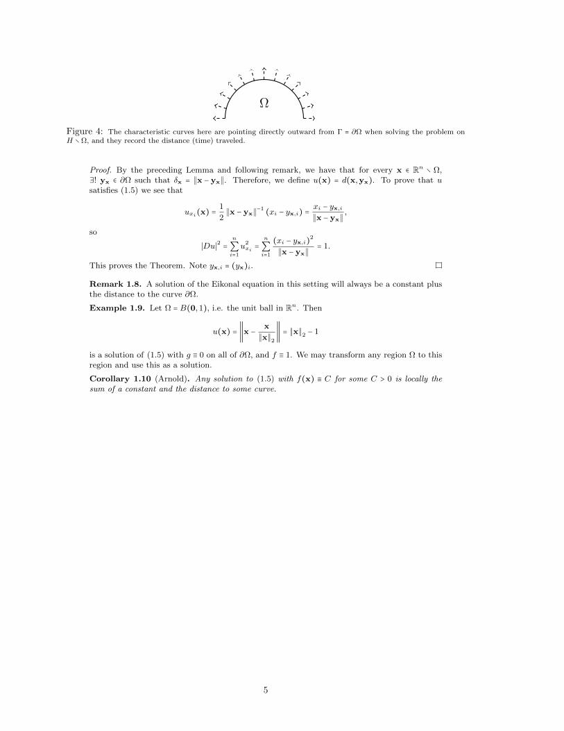
Ω
Figure 4: The characteristic curves here are pointing directly outward from Γ = ∂Ω when solving the problem onH ∖Ω, and they record the distance (time) traveled.
Proof. By the preceding Lemma and following remark, we have that for every x ∈ Rn ∖ Ω,∃! yx ∈ ∂Ω such that δx = ∥x − yx∥. Therefore, we define u(x) = d(x,yx). To prove that usatisfies (1.5) we see that
uxi(x) =1
2∥x − yx∥−1 (xi − yx,i) =
xi − yx,i∥x − yx∥
,
so
∣Du∣2 =n
∑i=1
u2xi =
n
∑i=1
(xi − yx,i)2
∥x − yx∥= 1.
This proves the Theorem. Note yx,i = (yx)i.
Remark 1.8. A solution of the Eikonal equation in this setting will always be a constant plusthe distance to the curve ∂Ω.
Example 1.9. Let Ω = B(0,1), i.e. the unit ball in Rn. Then
u(x) = ∥x − x
∥x∥2
∥ = ∥x∥2 − 1
is a solution of (1.5) with g ≡ 0 on all of ∂Ω, and f ≡ 1. We may transform any region Ω to thisregion and use this as a solution.
Corollary 1.10 (Arnold). Any solution to (1.5) with f(x) ≡ C for some C > 0 is locally thesum of a constant and the distance to some curve.
5
2 Method of Characteristics
This section sets up the Method of Characteristics exactly as Evans does in his text but givesextra detail in some cases. The method of characteristics is one approach to solving the Eikonalequation (1.5) and first order fully nonlinear PDEs.
2.1 Method of Characteristics statement
Our goal is to solve a PDE given by
F (Du,u,x) = 0 on Ωu = g in Γ ⊆ ∂Ω,
(2.1)
for some open Ω ⊆ Rn.
Our notation lets z(s) = u(x(s)) and pi(s) = uxi(x(s)), so we consider F (p, z,x). Then thesystem that we solve provided by the method of characteristics is given by
The above holds for all s in an interval I = [0, T ] for some T > 0 (i.e. the solutions will existlocally).
Ω
Inflow boundary
Outflow boundary
Figure 5: Characteristics emanating from the inflow boundary to the outflow boundary. The inflow boundary isn’tnecessarily Γ, but it is the smallest set Γ can be so that we can get full solutions in the above scenario (assuming noneof the characteristics curves intersect one another).
2.2 Method of Characteristics derivation
We seek a path x(s) in Ω defined by the nonlinear PDE, for which we have u(x(s)) solvesthe PDE along THAT line. The goal is to create these trajectories with initial conditionsx(0) = x0 ∈ Γ ⊆ ∂Ω so that we may gain intuition concerning the behavior of u. This techniqueallows us to ‘patch’ solutions together within some local neighborhood of a portion of Γ.
6
We now formally begin the derivation by letting u ∈ C2(Ω) be a solution to (2.1) and once againstating that we set
z(s) ≜ u(x(s)) and p(s) ≜Du(x(s)),where we aim to choose a x(s) that allow us to ‘easily’ compute z(s) and p(s). We writepi(s) = uxi(x(s)). Following Evans, we exam p(s) and use the “chain rule in higher dimensions”to get
pi(s) =n
∑j=1
uxixj (x(s))xj(s). (2.3)
As Evans remarks this is rather discouraging since it involves second derivatives. Our objectivewill be to get rid of the second derivative terms with a ‘smart selection’ of x(s). Now simplycompute ∂
The LHS of the above is a familiar expression, seen in (2.3). If we were to select xj(s) =Fpj (p(s), z(s),x(s)) then combining (2.3) and the above will produce that
2.2.1 Why do we only define boundary data on Γ ⊆ ∂Ω?
Suppose a characteristic passes through two different points on the boundary. If we are, forinstance, in the case when constant function values propagate along characteristics (e.g. thetransport equation), we must be positive that the boundary data matches. That is, if x(s) is acharacteristic and x0 ≠ x(s1) with both x0,x(s1) ∈ ∂Ω, we must ensure that g(x0) = g(x(s1)),otherwise we have a conflict. This will be seen in following examples.
2.2.2 PDE solution satisfies ODEs
These equations are extremely useful as they allow us to form a smooth system of solvableODEs, where all of the second derivative terms have vanished due to our ‘smart’ selection ofx(s). We now verify that these equations truly do produce solutions for Du and u:
Theorem 2.1 (Structure of characteristics ODEs). Let u ∈ C2(Ω) solve the nonlinear, first-order partial differential equation (1.1) in Ω. Assume x(⋅) satisfies (2.2)(c). If p(⋅) =Du(x(⋅))and z(⋅) = u(x(⋅)), then p(⋅) and z(⋅) solve the ODEs (2.2)(a) and (2.2)(b), respectively.
Proof. We have pi(s) = uxi(x(s)). Differentiating with respect to s yields
Boundary conditions are of interest since we aim to solve the ODE system to recover informationabout u. In the following subsection we illustrate that we may WLOG assume that our boundaryis ‘flat’ near our initial point x0 ∈ Γ ⊆ ∂Ω.
2.3.1 Straightening the boundary
Fixing x0 ∈ Γ, we “find” (Evans) smooth mappings Φ,Ψ ∶ Rn → Rn with Ψ = Φ−1 and Φ‘straightens out’ ∂Ω near x0.
We are now seeking a solution u ∶ Ω→ R to (1.1). Write Υ = Φ(Ω), setting
υ(y) ≜ u(Ψ(y)) ∀ y ∈ Υ,
and thenu(x) = υ(Φ(x)) ∀ x ∈ Ω.
We now illustrate that the PDE, call it G, associated with v is of the “same form” as the PDEfor u. Calculating the derivatives of u provides this information:
uxi(x) =n
∑j=1
vyj (Φ(x))Φjxi(x) ∀ i = 1, . . . , n.
Writing this in vector-matrix form, we see that
Du(x) =Dv(y)DΦ(x),
where y = Φ(x) and x = Ψ(y). Plugging this into (1.1) then provides us that
G(Dv(y), v(y),y) ≜ F (Dv(y)DΦ(Ψ(y)), v(y),Ψ(y)) = F (Du(x), u(x),x) = 0.
Defining v(y) = h(y) ≜ g(Ψ(y)) on Θ = Φ(Γ), we therefore have
G(Dv, v,y) = 0 in Υv = h on Θ.
2.3.2 Compatibility conditions
As shown in the previous section we may assume that for a given fixed x0 ∈ Γ, that it is flat onthe boundary – that is, it lies in the plane xn = 0.
How do we define our initial conditions correctly so that the ODE system truly produces solutionsalong characteristics? Carefully. We are given
p(0) = p0, z(0) = z0, x(0) = x0,
but only currently have defined x0. Since z(s) = u(x(s)), it seems natural that z(0) = u(x0) =g(x0). That is,
z0 = g(x0). (2.6)
The more complicated question we aim to answer is how to define p0. We know that u(x) = g(x)on Γ ⊆ ∂Ω. Since we assume that x0 lived in the plane with xn = 0, we then have that
uxi(x0) = gxi(x
0) ∀ i = 1, . . . , n − 1,
and since we also want the PDE to hold we finally have our compatibility conditions on p0:
pi0 = gxi(x0) ∀ i = 1, . . . , n − 1
F (p0, z0, x0) = 0.(2.7)
This gives n equations with n unknowns. Together (2.6) and (2.7) gives us what we call ourcompatibility conditions.
8
2.3.3 Non-characteristic boundary data
The objective of this section is to provide some groundwork for when we may solve a first-orderPDE using the method of characteristics, locally. We start with a fixed point x0 ∈ Γ. From(2.7) we have a way to define p0 given x0. We now pose conditions to solve for this initial valueproblem locally for all y ∈ Γ near x0. That is, we seek a function q(⋅) such that q(x0) = p0 andq(y) satisfies the comp ability conditions.
That is, we fix y ∈ Γ near x0 and we hope to solve the characteristic ODEs (2.2) subject to theinitial conditions
p(0) = q(y), z(0) = g(y), x(0) = y.
We then must figure out how to select q(⋅). It must satisfy q(x0) = p0 as well as the compatibilityconditions (2.7). To summarize, we must have
Lemma 2.2 (Noncharacteristic boundary conditions). There exists a unique solution q(⋅) of(2.8) for all y ∈ Γ sufficiently close to x0, provided
Fpn(p0, z0, x0) ≠ 0. (2.9)
Remark 2.3. The triple (p0, z0, x0) is said to be noncharacteristic if (2.9) holds.
Proof of Lemma 2.2. We are automatically provided the first n−1 components of q(y) by (2.8),so the goal is to solve for qn(y). Remembering that xn0 = 0, since we assumed flatness of theboundary, it makes sense that Fpn(p0, z0, x0) ≠ 0 should be an appropriate condition to ‘push’solutions out of the xn = 0 plane.
We aim to solve for qn(⋅) about (p0, z0, x0). To do do we must consider ∂F∂pn
(p0, z0, x0) and
show it is nonzero. This is given by the condition in (2.9), and hence by the implicit functiontheorem we may then solve for q(⋅) locally about x0.
2.4 Local existence
Theorem 2.4 (Local invertibility). Assume we have the noncharacteristic condition Fpn(p0, z0, x0) ≠0. Then ∃ interval I such that 0 ∈ I ⊆ R, and a neighborhood W of x0 in Γ ⊆ Rn−1, and aneighborhood V of x0 in Rn, and a neighborhood V of x0 in Rn, such that for each x ∈ V thereexist unique s ∈ I, y ∈W such that
x = x(y, s).The mappings x↦ s, y are C2.
W
V
x0y
x = x(y, s)
Ω
Figure 6: This diagram shows the local existence given by the inverse function theorem. We have a neighborhoodW of x0 on Γ ⊆ ∂Ω. We also then have a neighborhood V of x0 living in Ω ⊆ Rn. This solvability for the solutionu ∈ C2 will be given on V , and as such we have that the characteristics will not intersect in V .
9
Proof. With our notation we have x(x0,0) = x0. We will apply the Inverse Function Theoremwhich gives the result that we may solve for x = x(y, s).
First use thatx(y,0) = (y,0) (y ∈ Γ),
which gives
xjyi(x0,0) = δij (j = 1, . . . , n − 1)
0 (j = n).
We will use this to produce Dyx, an (n − 1) × (n − 1) matrix. In the s-component for each ofthese, we have that derivative is simply zero. We also have, directly from our characteristicequations (2.2)(c), that
xjs(x0,0) = Fpj (p0, z0, x0).
With all of this in hand we may write the Jacobian of x to prove the solvability of x with regardto the other variables of F . Since x depends on y and s, we have computed it’s derivative withrespected to those, and now collected them into the full Jacobian:
Dx(x0,0) =⎛⎜⎜⎜⎝
1 Fp1(p0, z0, x0)
⋱ ⋮1 ⋮
0 0 0 Fpn(p0, z0, x0)
⎞⎟⎟⎟⎠n×n
.
The determinant of the above is obviously nonzero so long as Fpn(p0, z0, x0) ≠ 0, our character-istic condition. The inverse function theorem now gives the result.
Remark 2.5. Assuming we have some y ∈ Γ close to x0, we will use the following notation toshow the dependence of solutions to the characteristic ODE not only on s, but on y as well.That is, not only on the time elapsed along the characteristic from the boundary, but also wherethat characteristic started from (which makes sense).
⎧⎪⎪⎪⎨⎪⎪⎪⎩
p(s) = p(y, s)z(s) = z(y, s)x(s) = x(y, s).
Sometimes it may also be written that x0 ∈ Rn−1 due to having assumed a straightened boundary(i.e. xn = 0).
Remark 2.6. The above lemma provides us that for each x ∈ V that we may uniquely solve
x = x(y, s)for y = y(x), s = s(x). (2.10)
Now we may solve
u(x) ≜ z(y(x), s(x))p(x) ≜ p(y(x), s(x)), (2.11)
for x ∈ V and s, y as in (2.10).
Theorem 2.7 (Local Existence Theorem). The function u defined above is C2 and solves thePDE
F (Du(x), u(x),x) = 0 (x ∈ V ),with the boundary condition
u(x) = g(x) (x ∈ Γ ∩ V ).
Proof. We attack the proof as follows:
(1) First we set up the problem: Fix y ∈ Γ near x0. Solve the characteristic ODEs (2.2) andwrite p(s) = p(y, s), z(s) = z(y, s), and x(s) = x(y, s) according to the previous work.
(2) Now we want to show that the PDE (1.1) is satisfied along the characteristics. That is,for y ∈ Γ ‘close enough’ to x0 ∈ Γ, then we want to show that
f(y, s) ≜ F (p(y, s), z(y, s),x(y, s)) = 0 (s ∈ I). (2.12)
10
We will proceed to show f(y,0) = 0 and fs(y, s) = 0, which directly implies f(y, s) = 0.First,
f(y,0) = F (p(y,0), z(y,0),x(y,0)) = F (q(y), u(y), y) = 0
by our compatibility condition (2.7). Also,
fs(y, s) =n
∑j=1
Fpj pj + Fz z +
n
∑j=1
Fxj sj
plug in (2.2)→ =n
∑j=1
Fpj [−Fxj − Fzpj] + Fz
⎛⎝
n
∑j=1
Fpjpj⎞⎠+
n
∑j=1
FxjFpj
= 0.
This shows, as mentioned, that f(y, s) = 0 as desired.
(3) Now by Lemma 2 and the resulting equations (2.10) and (2.11) along with the result (2.12)we finally have
F (p(x), u(x), x) = 0 ∀x ∈ V.Recall that V is the neighborhood about x0 for which we were able to solve (2.10) and(2.11). The above looks like what we desire, but we must formally prove that p(x) solvedvia the Local Invertibility Theorem is in fact Du(x). That is, we must show that
p(x) =Du(x) (x ∈ V ) (2.13)
To do so is slightly computationally complicated so we take a momentary detour.
Precomputations for final result. Let s ∈ I and y ∈ W . We have directlyfrom the characteristic ODEs that (don’t get confused here, z = zs and xj = xjssince we now have two variables (y, s) technically)
zs(y, s) =n
∑j=1
pj(y, s)xjs(y, s). (2.14)
We also will establish that
zyi(y, s) =n
∑j=1
pj(y, s)xjyi(y, s) (i = 1, . . . , n − 1). (2.15)
To do so define
ri(s) ≜ zyi(y, s) −n
∑j=1
pj(y, s)xjyi(y, s)
for each i = 1, . . . , n − 1. Taking the derivative of ri(s) with respect to s gives
ri(s) = zyis −n
∑j=1
(pjsxjyi + pjxjyis) (2.16)
Taking (2.14) and differentiating with respect to yi gives
zsyi =n
∑j=1
(pjyixjs + pjxjsyi) .
Placing this into (2.16) gives
ri(s) =n
∑j=1
(pjyixjs − pjsxjyi) =
n
∑j=1
[pjyiFpj − (−Fxj − Fzpj)xjyi] . (2.17)
We now differentiate (2.12) with respect to yi to get
n
∑j=1
Fpjpjyi + Fzzyi +
n
∑j=1
Fxjxjyi = 0.
Plugging this into (2.17) finally gives us that
ri(s) = Fz⎛⎝
n
∑j=1
pjxjyi − zyi⎞⎠= −Fzri(s).
Since ri(s) solves the above ODE with initial condition ri(0) = gxi(y)−qi(y) = 0,
this clearly gives ri(s) ≡ 0 for all s ∈ I and i = 1, . . . , n − 1. This proves (2.15).
11
Now we may proceed. To keep notation simple, let j = 1, . . . , n, and using (2.11) we have
uxj = zssxj +n−1
∑i=1
zyiyixj
by previous work→ =n
∑k=1
pkxkssxj +n−1
∑i=1
n
∑k=1
pkxkyiyixj
=n
∑k=1
pk (xkssxj +n−1
∑i=1
xkyiyixj)
=n
∑k=1
pkxkxj =n
∑k=1
pkδjk = pj .
That is, p =Du.
2.5 Examples
2.5.1 Eikonal equation
The Eikonal equation can be written as
F (p, z,x) = −f(x) + 1
2
n
∑i=1
p2i = 0,
so we may solve it via the method of characteristics. We have xi = pi, pi = −fxi , and z = ∣p∣2 fori = 1, . . . , n.
This gives thatx(s) =Du(x(s)),
so we may think of a characteristic emanating from Γ ⊆ ∂Ω to be moving in the “directionof optimal motion,” the direction of the gradient at that position. The exact dynamics arecontrolled by our choice of f . For polynomial f of degree 2 or less, the characteristic ODEsystem is fully linear (except for z, but that isn’t involved in the coupling between x and p)and we may solve it using standard ODE techniques. Once f becomes nonlinear, the problemobviously becomes harder.
2.5.2 Examples: Deriving PDEs from conditions on characteristics
Let U ⊆ Rn be open with ∂U smooth. Suppose we have F ∶ Rn ×RU , F (p, z,x) is smooth andg ∶ Γ→ R is also smooth on Γ ⊆ ∂Ω.
From the Local Existence Theorem of the Method of Characteristics, we have that ∃V ⊆ U ,a neighborhood of Γ so that the method of characteristics has produced a C2 solution, u(x)satisfying (1.1).
For these problems we consider that our vector field
v ∶ Rn → Rn, v = v(x)
is smooth and transversal to Γ.
Example 2.8 (Time-optimal problem). We seek solutions to (1.1) such that the time traveledalong a characteristic gives the value of the function. That is, u(x(s)) is the time traveled alongx(s) since entering U . This gives us obvious boundary data: g ≡ 0 on Γ = ∂U .
First we suppose that our characteristics follow according to the vector field v(x). This placesthe condition on F that
v(x) =Dp(Du(x), u(x),x) (2.18)
immediately (it places the condition along each characteristic, so assuming it for the whole spaceis okay).
12
To start, we writez(s) = u(x(s)) = s Ô⇒ z(s) = 1,
and since z(s) = x ⋅ p = v ⋅ p, we therefore arrive at
v ⋅ p = 1, (2.19)
as an obvious condition our PDE must satisfy. Remember that v(x) = DpF (Du(x), u(x),x)is something F must satisfy. After careful inspection notice that F (Du(x), u(x),x) = v(x) ⋅Du(x)− 1 is an obvious candidate satisfying both (2.18) and (2.19) so we have derived a PDE.
Note that if we select v(x) =Du(x) we rederive the Eikonal equation.
Homework problem 1. Using the same approach, derive a PDE such that u(x(s)) is thetotal distance traveled from x(0) ∈ Γ along each characteristic x(s).
Homework problem 2. Can you do the same thing to derive a PDE that satisfies u(x(s)) =g(x(0)) on each characteristic?
2.5.3 Examples of how characteristics flow
The following examples come directly from Evans. We provide some discussion about certainsimple scenarios in which we could construct PDEs to satisfy the given properties.
Flow to an attracting point. If we consider a situation in which the characteristics flow to anattracting point, we may think of our vector field x(s) = v(x(s)) =DpF (Du(x(s)), u(x(s)),x)as having a single critical point and on the entire vector field we have v ⋅ ν < 0 where ν is theoutward pointing normal.
Figure 7: Flow to an attracting point. Figure copied directly from Evans.
It is a fair question to ask if solutions constructed using the method of characteristics will besmooth, or even continuous. In this case the answer is no, that they will not be smooth, andunless U itself is a ‘very’ nice shape (e.g. a circle) we will likely even have discontinuities indifferent values leading up to the critical point.
Further, consider the preceding example where the solution u returns the amount of time trav-eled along each characteristic. The characteristics themselves never reach the critical point(standard ODE theory), and hence it takes infinite time. Thus if w is the critical point, thenu(x)→∞ as x→w.
On the other hand, if we were to instead consider the PDE giving the amount of distance trav-eled, this would produce finite, but likely discontinuous solutions (certainly not smooth).
13
Figure 8: Flow across a domain (left) and a characteristic point given by D (right). Figures copied directly fromEvans.
2.6 Characteristics for Hamilton-Jacobi equations
The characteristics for the Hamilton-Jacobi equations provide a coupling in the characteristicequations between the x and p, with no dependence on z = u. The general Hamilton-JacobiPDE is given by
G(Du,ut, u, x, t) = ut +H(Du,x) = 0,
with Du =Dxu. If we let y = (x, t), q = (p, pn+1), this gives
G(q, z, y) = pn+1 +H(p, x)
for the PDE we’ll apply the Method of Characteristics to. We result in
The first and third of these give Hamilton’s equations. These equations give a nice couplingbetween p and x, with no z terms. z depends on p and x exclusively, so once those are solvedwe have solved the problem.
2.7 One true MoC example
Just to show how we may apply the Method of Characteristics to a real and given problem, weconsider Problem 5(c), a quasi-linear PDE:
uux1 + ux2 = 1 with u(x1, x1) =1
2x1.
To solve this write the PDE in standard form:
F (p, z, x) = zp1 + p2 − 1 = 0.
Using the method of characteristics we determine
z = x ⋅ p = (z,1) ⋅ (p1, p2) = 1, p1 = −0 − p1 ⋅ p1
p2 = −0 − p1p2, x1 = zx2 = 1.
14
Selecting x0 = (t, t), we then have g(x0) = 12t. for t ∈ R. We may solve that z(s) = s + z0 =
s + g(x0) = s + 12t, so
x1 = s +1
2t Ô⇒ x1(s) =
1
2s2 + 1
2st + x0
1 =1
2s2 + 1
2st + t,
and x2(s) = s + x02 = s + t. Now, we have
(1
2s2 + 1
2st + t, s + t) = (x1(s), x2(s)) ,
and solving for s, t we arrive at
(s, t) = (2x2 − 2x1
2 − x2,2x1 − x2
2
2 − x2) .
This finally allows us to get rid of the s to produce
u(x1, x2) = s +1
2t = −x1 + 2x2 − x2
2/22 − x2
.
15
3 Calculus of Variations vs. Optimal Control
This section aims to provide a (more or less) definition of what calculus of variations and op-timal control exactly are and how they are related. Calculus of variations seeks to minimize afunctional over a set of trajectories in the state space starting at one location and ending atanother, in finite time.
Optimal control problems are a subset of calculus of variations problems, yet we have a dynam-ical “control” placed on the derivatives of all elements in the admissible class A.
3.1 Calculus of Variations
We let L ∶ Rn × Rn → R be a smooth function named the Lagrangian. Fix any two pointsx, y ∈ Rn with x ≠ y and select t > 0. We define the action functional
I[w(⋅)] ≜ ∫t
0L [w(s),w(s)]ds,
where the functions w belong to the admissible class
A ≜ w(⋅) ∈ C2 ([0, t];Rn) ∣ w(0) = y, w(t) = x .
A problem in the calculus of variations is to minimize this action functional over A. I.e. weseek x(⋅) so that
I [x(⋅)] = minw(⋅)∈A
I[w(⋅)].
t0
time
Rn w(⋅) x(⋅)
Figure 9: A problem in calculus of variations is to minimize a functional I[w(⋅)] = ∫t
0 L(w(s),w(s))ds over all
possible candidates w(⋅) ∶ [0, t] → Rn satisfying that w ∈ C2 ([0, t]) and w(0) = x and w(t) = y. Here x(⋅) is theminimizer.
3.2 Optimal Control
In optimal control we now prescribe our set A of admissible candidates to satisfy an additionaldynamic control. Any w(⋅) ∈ A must now also satisfy the system
w′(s) = f(w(s),a(s)) in Ω ⊆ Rnw(0) = x for some fixed x ∈ Ω.
Our goal is still the same. We are starting at an initial point x at time zero and traveling tosome other point, w(t) = y.
Rather than dwell on the details, let’s see this in action:
16
3.2.1 Deriving the Eikonal equation (Optimal Control)
Deriving the Eikonal equation from an optimal control problem is a simple yet elegant result.
Define the trajectory of motion to be given by y(s) for s ∈ [0, T ] for some T > 0, where
y′(s) = f(y(s))a(s) in Ωy(0) = x for some fixed x ∈ Ω.
That is, y(s) is a trajectory living in Ω, where a(⋅) is our ‘control’ with a ∶ R→ A ⊆ Rn, with Acompact and contained in the unit sphere. That is, ∣a(⋅)∣ = 1 for all a(⋅) ∈ A.
We consider that as the trajectory y(s) moves it accrues a cost presented by the cost functionK(x,a(⋅)), where K ∶ Ω ×R → R. Once y(s) ∈ ∂Ω for the first time, we incur an exit-cost givenby the function q ∶ ∂Ω→ R.
T (x,a(⋅))
T (x,b(⋅))
Ω
x
Figure 10: The curve in red represents y(t) given by the trajectory of motion. The speed at any point in Ω is
controlled by f , and direction by a(⋅). We will later see that we will choose a(x) = −∇u(x)∣∇u(x)∣ for all x ∈ Ω, i.e. the
direction of maximal decrease. We may think of the curve in red as the curve with this select of control. Should wepick another control b(⋅) we would get a different curve, e.g. the blue one.
Define the final exit time starting at x to be given by
T (x,a(⋅)) = mint ≥ 0 ∣ y(t) ∈ ∂Ω .
Now, the total cost to exit starting at x is then given by
J (x,a(⋅)) = ∫T (x,a(⋅))
0K(y(s),a(s))ds + q(y(T (x,a(⋅)))).
Finally, we choose to infemize over all possible controls a(⋅) in order to produce the valuefunction, which returns the minimal exit cost starting at x:
v(x) = inf∣a(⋅)∣=1
J (a,a(⋅)).
This looks like an intimidating beast to tackle right off the bat. We appeal to Bellman’s opti-mality principle, which gives us the following. Let τ > 0 be a ‘small’ number. By the principle
17
if we travel along y(s) for τ seconds, we accrue cost according to K, and we wish to add on theminimal-cost-to-exit at y(τ), given by b(y(τ)). To summarize,
v(x) = inf∣a(⋅)∣=1
[∫τ
0K(y(s),a(s))ds + v(y(τ))] .
Since τ > 0 is small, the integral term may be approximated using geometry:
Plugging all of this into the equation we now have
v(x) = inf∣a(⋅)∣=1
[τK(x,a(0)) + v(x) + τf(x)∇v(x) ⋅ a(0) +O(τ2)]
= v(a) + τ inf∣a(⋅)∣=1
[K(x,a(0)) + f(x)∇v(x) ⋅ a(0) +O(τ)] .
Canceling v(x) on each side and dividing through by τ , we are left with (inf = min since A iscompact)
min∣a(⋅)∣=1
[K(x,a(0)) + f(x)∇v(x) ⋅ a(0)] +O(τ).
We may assume that K = K(x) (i.e. it only depends on physical location) in order to deduce
that selecting a∗(0) = − ∇v(x)∣∇v(x)∣ is the minimizer. Taking τ ↓ 0 we are finally left with
K(x) − ∣∇v(x)∣ f(x) = 0 Ô⇒ ∣∇v(x)∣ =K(x)/f(x).
Taking K ≡ 1 is a standard procedure.
18
4 References[A] Lectures on Partial Differential Equations, by Vladimir Arnold[E] Partial Differential Equations, by Lawrence Evans (second edition)[K] Introductory Functional Analysis with Applications, by Kreyszig[S] 300 Years of Optimal Control: From The Brachystochrone to the Maximum Principle,