MBA 203 Executive Summary

MBA 203 Executive Summary

Matteo Benetton & Anastassia Fedyk

* This Executive Summary is an older version from a previous course offering. The document isintended to help students during the Fall 2021 waiver exam period.

While the course content may be similar, another faculty will be teaching this course in Fall 2021 so the content will likely be different than this sample summary.

Recap

Matteo Benetton - Introduction to Finance - 2019

• Class 1: Present and future value

• Class 2: Present and future value, continued• Class 3: Capital budgeting: The decision rule

• Class 4: Capital budgeting: The cash flow• Class 5: Stocks• Class 6: Bonds

• Class 7: Bonds, continued• Class 8: Portfolio choice

• Class 9: Portfolio choice, continued• Class 10: Portfolio choice, continued• Class 11: The CAPM

• Class 12: Applying the CAPM: Evidence, extensions. Assessing fund performance & market efficiency• Class 13: Applying the CAPM: Estimating the cost of capital for an equity-financed project

• Class 14: Capital structure

Present and Future Value


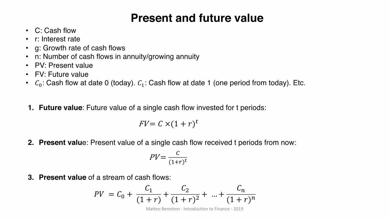
• C: Cash flow• r: Interest rate• g: Growth rate of cash flows• n: Number of cash flows in annuity/growing annuity• PV: Present value• FV: Future value• !": Cash flow at date 0 (today). !#: Cash flow at date 1 (one period from today). Etc.

1. Future value: Future value of a single cash flow invested for t periods:

2. Present value: Present value of a single cash flow received t periods from now:

3. Present value of a stream of cash flows:

FV= ! ×(1 + ,).

PV= 0(#12)3

45 = !" +!#

(1 + ,) +!6

(1 + ,)6 + …+ !8(1 + ,)8

Present and future value


4. Perpetuity: Future value of a single cash flow invested for t periods:

5. Growing perpetuity: Present value of a single cash flow received t periods from now:when r-g >0

6. Annuity: of a stream of cash flows:

7. Growing annuity: of a stream of cash flows:

when r<g or r>g

8. Future value of a perpetuity, growing perpetuity, annuity, or growing annuity as of later date t:

9. After tax cash flows and interest rates at tax rate t:

10.Excel function: NPV

PV= %&'(

PV= %& 1 − +

(+-&)/

PV= %&'( 1 − +-(

+-&0

FV= 23 ×(1 + 6)0

789:;&':<= = 1 − > ×7?;9@&;':<=689:;&':<= = 1 − > ×6?;9@&;':<=

PV= %&


• !"#$%& : Real cash flow at date t

• !"'()*'%& : Nominal cash flow at date t

• +#$%&: Growth rate of real cash flows

• +'()*'%& : Growth rate of nominal cash flows

• ,#$%& : Real interest rate

• ,'()*'%& : Nominal interest rate

• -: The rate of inflation

• k : Number of compounding periods per year

• APR: Annual percentage rate

• EAR: Effective annual rate

Practical issues

1. Nominal vs. real cash flows: (i is the expected inflation rate)

Growth rates of real and nominal cash flows:

Nominal vs. real interest rates:

Discounting real cash flows at the real interest rate or nominal cash flows at the nominal interestrate gives the same present value:

2. Interest rate per compounding period:

Effective annual rate (EAR): If you invest $1 at APR with compounding k times per year, then after one year you haveand after t years you have (1 + $%&)( .


)* =,-./01.23

(456./01.23)-= ,-

./01.23/(459)-

(456./01.23)-/(459)-=

,-:;23

(456:;23)-

<=>69?@ =%)&

A

B(6>CD =

B(E?F9ECD

(1 + G)(

1 + H6>CD =1 + HE?F9ECD

1 + G

1 + <6>CD =1 + <E?F9ECD

1 + G

1 + $%& = (1 + <=>69?@)I

3. Dealing with cases with multiple interest rates:

• Calculate loan payments using the loan interest rate

• Calculate the principal still owed by discounting the remaining payments using the loan interest rate

• Calculate present value (market value) using the going market rate.

4. Excel functions: PV, PMT, FV, NPER, RATE (all for annuities), SOLVER.


Capital budgeting

Decision rule

1. The net present value (NPV) of a project’s cash flows is:

The NPV decision rule:

(a) For a single project, or several independent projects, accept the project if and only if NPV > 0.

(b) For mutually exclusive projects, accept the project with the highest NPV, provided that project’s NPV > 0.

!"# = %& +%(

(1 + +) +%-

(1 + +)- + …+ %/(1 + +)/

Decision rule

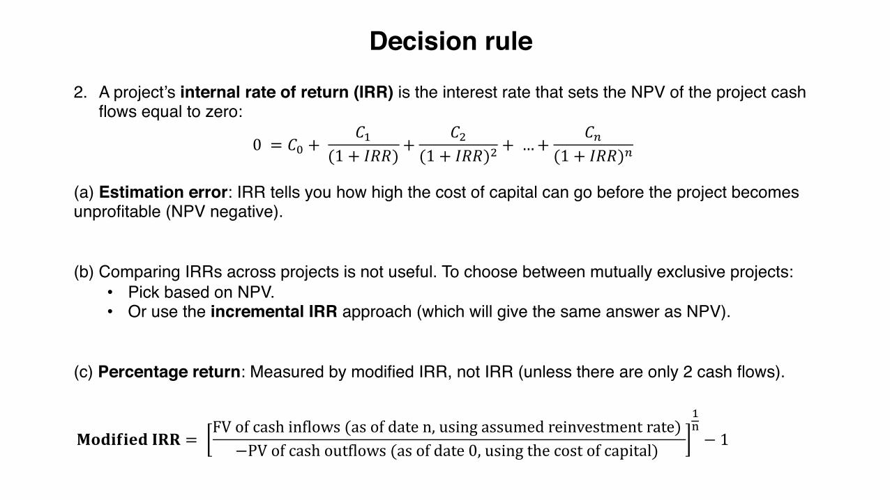
2. A project’s internal rate of return (IRR) is the interest rate that sets the NPV of the project cash flows equal to zero:

(a) Estimation error: IRR tells you how high the cost of capital can go before the project becomes unprofitable (NPV negative).

(b) Comparing IRRs across projects is not useful. To choose between mutually exclusive projects:• Pick based on NPV.• Or use the incremental IRR approach (which will give the same answer as NPV).

(c) Percentage return: Measured by modified IRR, not IRR (unless there are only 2 cash flows).

0 = #$ +#&

(1 + )**)+

#,

(1 + )**),+ …+

#.

(1 + )**).

/0123241 566 =FV of cash inAlows (as of date n, using assumed reinvestment rate)

−PV of cash outAlows (as of date 0, using the cost of capital)

&P

− 1

Decision rule

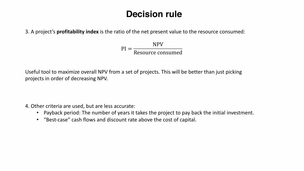
3. A project’s profitability index is the ratio of the net present value to the resource consumed:

PI = NPVResource consumed

Useful tool to maximize overall NPV from a set of projects. This will be better than just pickingprojects in order of decreasing NPV.

4. Other criteria are used, but are less accurate:• Payback period: The number of years it takes the project to pay back the initial investment.• “Best-case” cash flows and discount rate above the cost of capital.

The cash flow

Matteo Benetton, Introduction to Finance, 2019

Free cash flow, !": How much cash physically flows to/from the firm (or project) and is available topay investors/must be provided by investors after all other obligations are met.

C% = 1 − τ* × Revenues% − Cost% − De56789:;9<=%

>?@AB

CDEFGFHFI JFK LDMNOFB

+De56789:;9<=% − Q7; 8:59;:R 7S57=T9;U67%−(Operating working capital% − Operating working capital%ab)

• τ* is the corporate tax rate• Operating working capital = Inventory + Accounts Receivable − Accounts Payable• Sale of capital enters as negative capital expenditure, and remember taxes:

After-tax cash flow from asset sale = Sale price − τ× (Sale price−Book value)

where the book value is the amount of the purchase price that has not yet been depreciated.

• If EBIT is negative in a particular year, you should still multiply by (1− τ) if the firm has sufficient profits from other projects. If not, you need to deal with tax carrybacks/carryforwards.

Discounted cash-flow valuation


Step 1: PV as of end of 2012 of the cash flows from 2013-2018:

!" =$%&'(1 + + +⋯+

$%&'-1 + + . = $95.5435

Step 2: Terminal value at the end of 2018:6+77 89:ℎ <=>?%&'@

+ − B=(1 + B)×6+77 89:ℎ <=>?%&'-

+ − B= $446.7385

Step 3: Discount the terminal value back to end of 2012:

!" =$446.73851 + + . = $225.1235

Step 4: The stock price is then:

JK>8L M+N87 =OPK7+M+N:7 Q9=R7Jℎ9+7: >RK:K9PSNPB =

$95.5435 + $225.12359.945 = $32.24 M7+ :ℎ9+7

Stock price as of end of 2012: Based on value of free cash flows from 2013-2018, the terminal value as of 2018 and the number of shares.

Stocks and bonds

Stocks


1. Dividend discount model: The price of a stock is the PV of its expected future dividends per share

2. Dividend discount model with constant growth: Assumptions: (a) The number of shares is constant (no issues or repurchases), (b) the firm has no debt or cash, (c) the return on new investment is constant, and (d) absent any new investments, earnings would be constant over time. Then:

• !"#$ = !&'&()*( +,-./0 1,0) × 345$• 6 = 7)0)*0&.* 1,0) × 7)0/1* .* *)8 &*')90:)*0• !&'&()*( +,-./0 1,0) + 7)0)*0&.* 1,0) = 1

3. Free cash flow model:

Enterprise value0 is the PV of the free cash flows. To calculate enterprise value make sure to use the firm’s overall cost of capital (the weighted-average cost of capital), not just it’s equity cost of capital (more on this later in the class).

4= =>?@$

A!"#?

(1 + 1)?

4= =!"#$1 − 6

4= =3*0)1+1&9) ',E/)= + F,9ℎ= − !)H0=

5ℎ,1) ./090,*(&*6=

Stocks


4. Total payout model:

where (under constant growth):• !" #$%$&' %(%)* +,-,+'.+/ ).+ &'0$&1ℎ)/'/ =

45678 9:;:9<=9> 7=9 ?<@A?BC7><> 76 6:D< E

?FG

• H = I'%'.%,(. &)%' × I'%$&. (. .'K ,.-'/%L'.%• M,-,+'.+ 0)N($% &)%' + I'%'.%,(. &)%' + I'0$&1ℎ)/' &)%' = 1

5. Multiples valuation: Using the multiple Enterprise value/Free cash flows as an example:

• Carefully chosen multiple:Multiples based on free cash flows rather than a number “higher up” such as net income or sales are more likely to be similar.

• Carefully chosen comparable firms:Since the multiple depends on the firm’s growth profile and cost of capital we need to pick comparable firms for which this is likely to be true.

!Q =!"(#$%$&' %(%)* +,-,+'.+/ ).+ &'0$&1ℎ)/'/)

Tℎ)&' ($%/%).+,.H )% %,L' 0

V.%'&0&,/' -)*$'WQEXY:?D =

V.%'&0&,/' -)*$'

#&'' 1)/ℎ Z*(K WQEX

[;G. ]5? B5D@7?7^8< ]:?D>

×#&'' 1)/ℎ Z*(KWQEXY:?D

• F: Face value of bond, paid at maturity, in $• !" : Price today of an n-year zero coupon bond• #" : Yield today of an n-year zero coupon bond• C: Coupon payment, in $• c: Coupon rate, in percent• $" : Price today of an n-year coupon bond • #"%&'(&": Yield today of an n-year coupon bond.

1. Price of a n-year zero coupon bond with face value F:

This formula also defines the yield to maturity on the n-year zero coupon bond, #", as the (constant)discount rate that equates the discounted cash flow to the price. Reorganizing:

Bonds


!" =*

(1 + #")"

#" =*!"

/" − 1

Bonds


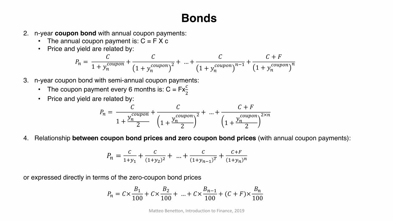
2. n-year coupon bond with annual coupon payments:• The annual coupon payment is: C = F X c• Price and yield are related by:

3. n-year coupon bond with semi-annual coupon payments:• The coupon payment every 6 months is: C = Fx!"• Price and yield are related by:

4. Relationship between coupon bond prices and zero coupon bond prices (with annual coupon payments):

or expressed directly in terms of the zero-coupon bond prices

#$ =&

1 + )$!*+,*$+ &

1 + )$!*+,*$" + …+ &

1 + )$!*+,*$$./ +

& + 01 + )$!*+,*$

$

#$ =&

1 + )$!*+,*$

2+ &

1 + )$!*+,*$

2" + …+ & + 0

1 + )$!*+,*$

2"×$

#$ = 3/456

+ 3/457 7 + …+ 3

/45896 : +34;/458 8

#$ = &× </100 + &×

<"100 + …+ &×<$./100 + (& + 0)× <$

100

5. PVs of riskless cash flow streams (when the term structure is not necessarily flat):

• Method 1: Price of zero coupon bonds à

• Method 2: Yields of zero coupon bonds à

6. For bonds with default risk

Bonds


!"# = %& +%(

1 + *(+

%+1 + *+ + + …+

%-.(1 + *-.( / +

%-1 + *- -

!"# = %& + %(×1(100

+ %+×1+100

+ …+ %-.(×1-.(100

+ %-×1-100

"3456 =7(%()1 + 7(3)

+7(%+)

1 + 7(3) + + …+7(%-) + 7(:)1 + 7(3) -

"3456 = ;<=>?@ABCD

(EF+ ;G

=>?@ABCD

(EF G + …+ ;H=>?@ABCDE I=>?@ABCD

(EF H

Optimal Portfolio Choice



1. Properties of portfolios of two risky assets A and B:

Correlation: !",$ = &'((*+,*,)(-+-,)

2. Minimum variance frontier (MVF): The relation between of E 01 and 21 when working with risky assets. (The set of risky portfolios with the lowest standard deviation for their expected return. But with only two risky assets, there’s only one possible 21 for each E 01 .

Portfolio weights: 3" + 3$ = 1Realized return: 01 = 3"0" + 3$0$Expected return: E(01) = 3"6(0") + 3$6(0$)Variance: 217 = 3"72"7 + 3$7 2$7 + 23"3$9:;(0", 0$) = 3"72"7 + 3$7 2$7 + 23"3$!",$2"2$Standard deviation: 21 = 217



0.00

0.02

0.04

0.06

0.08

0.10

0.12

0.00 0.05 0.10 0.15 0.20

Expe

cted

Ret

urn

Standard Deviation

Minimum Variance Frontiers

A

B Correlation=1

Correlation=-1

• For !",$ = 1 there is no diversification benefit'() = *")'") + *$) '$) + 2*"*$!",$'"'$ = (*"'" + *$'$)) → '( = *"'" + *$ '$

• For !",$ < 1 there is a diversification benefitA portfolio of A and B will have '( < *"'" + *$ '$

3. Properties of portfolios of a riskless asset f and a risky asset A:

4. Capital allocation line (CAL): The relation between of E "# and $# when working with a risky and a riskless asset. On the CAL:

Intercept: The riskless interest rate. Slope: Sharpe ratio of the risky asset.



Portfolio weights: %& + %( = 1Realized return: "# = %&"& + %("(Expected return: E("#) = %&-("&) + %("(Variance: $#. = %&.$&.Standard deviation: $# = %&$&

E "# = "( +- "& − "(

$&$#

5. Optimal portfolio choice with a riskless asset and two or more risky assets:

• The best portfolio of risky assets to combine the riskless asset with is the one that leads to the steepest CAL (less risk for same expected return/higher expected return for same risk), i.e., which has the highest Sharpe ratio. It called the mean-variance efficient (MVE) portfolio of risky assets, or the tangency portfolio.



0.00

0.02

0.04

0.06

0.08

0.10

0.12

0.00 0.05 0.10 0.15 0.20

Expe

cted

Ret

urn

Standard Deviation

Capital Allocation Line (CAL)

A

f



0.00

0.02

0.04

0.06

0.08

0.10

0.12

0.00 0.05 0.10 0.15 0.20

Expe

cted

Ret

urn

Standard Deviation

A

B

• In the case of two risky assets, you can find the MVE portfolio of risky assets using SOLVER in excel

• The resulting CAL is the optimal capital allocation line (CAL): The relation between of ! "# and $# when investing in the riskless asset and the MVE.

On the optimal CAL:

and therefore:

• Efficient portfolios lie on the optimal CAL and combine f and MVE. All (smart) investors should choose an efficient portfolio. The exact point chosen depends on how risk averse the investor is.



! "# = &'()! "'() + &+"+$# = &'()$'()

E "# = "+ +! "'() − "+

$'()$#

1. The four steps of portfolio choice

1. Collect data for each asset class. Estimate means, standard deviation, correlations

2. Calculate the optimal mix of the risky asset classes. The (MVE). Using SOLVER in excel

3. Decide how much you want to invest in risky assets (the MVE) and how much in the riskless asset (e.g. a money market fund)

4. Work out how many dollars you have invested in each asset class and the riskless asset

2. Adding more risky assets improves the minimum variance frontier of risky assets. We do not solve for the MVE in cases with more than two risky assets, but once you have the MVE portfolio of risky assets, everything works as in the case with two risky assets (and a riskless asset).





• Equal-weighted portfolios of risky assets, !" = !# = 1/n. • If all assets have the same variance $% and the same correlation &. Then any two risky assets have

the same covariance, cov= &$% . Then, the n-asset portfolio variance simplifies to:

• In general, let $% be the average variance and '() be the average covariance.

$*% = ,- $

% + -/,- &$% → &$% as n gets large

$*% =12 $

% + 2 − 12 '() → '() as n gets large

Diversifiable risk

Undiversifiable risk

The CAPM

• Equilibrium: Asset prices must adjust to ensure that

MVE Portfolio of risky assets = Market Portfolio of risky assets

• Capital market line (CML): The capital allocation line for investing in the riskless asset and the market portfolio of risky assets. On the CML:

Combining these,

The CAPM


12 = 13 + 56 (16 − 13)

E 12 = 13 + 56 (: 16 − 13)

;2 = 56;6

E 12 = 13 +< => ?=@

A>;2

• Capital asset pricing model (CAPM):A model of what the expected return on a security i will be in equilibrium. According to the CAPM

! is a regression coefficient in this regression:

If the expected return on any asset i differed from the above, the market portfolio would not be mean-variance efficient and the supply of risky assets would not equal the demand for risky assets.

• Security market line (SML):Illustrates the CAPM by plotting the formula E #$ = #& + !$ () #* − #&) to show that a security’s

expected return depends linearly on its b Matteo Benetton, Introduction to Finance, 2019

E #$ = #& + !$ () #* − #&)

#$,& − #&,. = /$ + !$ #*,. − #&,. + 0$,.

!$ =123(#$,. − #&,. , #*,. − #&,.)

4(#*,. − #&,.)

The CAPM

• Comparing the CML and SML:

• ! of a portfolio of " assets:

On the CML: !# = %&


!# = %'!' + %)!) + ⋯+ %+!+

-0.020.000.020.040.060.080.100.120.140.160.180.20

0.0 0.1 0.2 0.3 0.4Standard Deviation

Tiffany

TargetWalmart

Riskless

Market

Capital Market Line (CML)

Wholefood

-0.020.000.020.040.060.080.100.120.140.160.180.20

0 0.5 1 1.5 2

Expe

cted

Ret

urn

Beta

Security Market Line (SML)

Wholefood

RisklessWalmart

Target

Market

Tiffany

The CAPM

1. Understanding one data point:!",$ − !$,& = (" + *" !+,& − !$,& + ,",&

• !",$ − !$,&: The excess return on firm i in period t. What we’re trying to understand

• (": Intercept. An unexplained “boost” to/reduction in the return in each period

• *" (!+,& − !$,&): The part of !",$ − !$,& that is explained by the market (excess) return. The market (= systematic) component.

• ("+*" (!+,& − !$,&) Predicted value. What you’d predict !",$ − !$,& to be, given market’s excess return in this period.

• ,",&: Error term. The part of !",$ − !$,&that is not explained by the regression. The firm-specific (= diversifiable) component. Averages to zero across stocks for each t. Averages to zero for each stock across t (as in any regression)

More on the CAPM


2. Understanding mean returns:! "#,% = '# + "),% + *# ! "+,% − "),%

The expected return of a particular security comes from:• The riskless rate, "),%• A risk premium, driven by the market’s risk premium and the security’s beta: *# ! "+,% − "),%• Any unexplained boost to/reduction in returns, '#.

The CAPM claims that all securities should have '# = 0 and plot on the SML.

3. Understanding return variances:- ("#,% − "),%) = *#0 - "+,% − "),% + -(1#,%)

If the riskless rate is constant over time (or you look at variance given what’s known at time t):- ("#,%) = *#0 - "+,% + -(1#,%)

The risk of a particular security comes from:• Volatility of the market and the stock having a non-zero beta: Market risk, *#0 - "+,% − "),%• Volatility of the firm-specific component of the return: Firm-specific risk, -(1#,%)


More on the CAPM

The regression’s R2 measures what fraction of the total variance is due to market risk:

!"# =Explained Variance

Total Variance= Market Risk

Total Risk= %"# & '(,* − ',,*

& ('",* − ',,*)= %"# & '(,* − ',,*%"# & '(,* − ',,* + &(0",*)

The CAPM claims that &(0",*) is irrelevant for what expected return investors require on security i.

4. Multi factor models: The Fama French Carhart 4-factor model is the leading multi-factor model. Estimate betas in this regression:

'",* − ',,* = 1" + %",2('(,* − ',,*) + %",#('3(455,* − '6"7,*)+%",8 '9"79,* − '5:;,* + %",< ';"==>?3,* − '5:3>?3,* + 0",*

Then expected returns are given by:@('") − ', = %",2(@('(,*) − ',) + %",#(@('3(455) − @('6"7))+%",8 @('9"79) − @('5:;) + %",< @(';"==>?3) − @('5:3>?3)


More on the CAPM

5. Markets are efficient (informationally) if prices reflect relevant information about cash flows and discount rates. To consider how efficient markets are we distinguish between:• Semi-strong form efficiency: You cannot make abnormal (risk-adjusted) returns by trading based

on public information.• Strong form efficiency: You cannot make abnormal (risk-adjusted) returns by trading basedon any

type of information (public or private).

6. Alpha (!): The difference between a security or portfolio’s actual expected return and what the expected return should be given the risk, according to our asset pricing model. Using the CAPM as our asset pricing model " is the vertical distance to the SML:

"# = %('#) − ('* + ,# %('- ) − '* )

You estimate the "# as the intercept in the CAPM regression:

.'# − (.'* + ,# '- − .'* )


More on the CAPM

If the CAPM is the right way to adjust for risk and markets are (informationally) efficient:

• Alphas of all investors and investment strategies should be (insignificantly different from) zero.

If markets are not efficient and you find an investment with (significantly) positive alpha:

• Calculate the MVE mix of the investment and the market portfolio of risky assets. Then invest in a mix of the riskless asset f and the MVE.


More on the CAPM

Implementing the CAPM to get the cost of capital


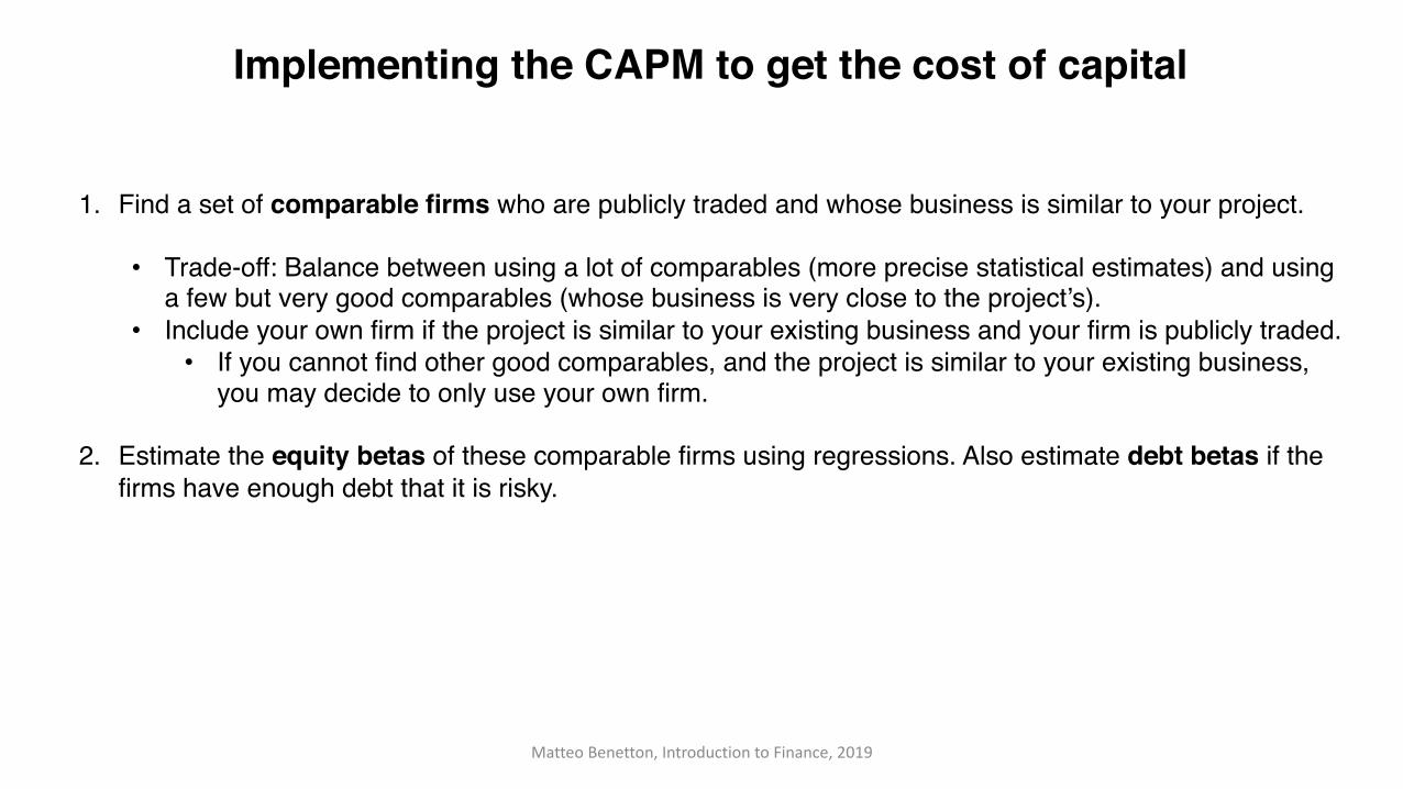
1. Find a set of comparable firms who are publicly traded and whose business is similar to your project.

• Trade-off: Balance between using a lot of comparables (more precise statistical estimates) and using a few but very good comparables (whose business is very close to the project’s).

• Include your own firm if the project is similar to your existing business and your firm is publicly traded.• If you cannot find other good comparables, and the project is similar to your existing business,

you may decide to only use your own firm.

2. Estimate the equity betas of these comparable firms using regressions. Also estimate debt betas if the firms have enough debt that it is risky.


3. For each comparable firm, i, calculate the asset beta: !"# = %&'& !%

# + )&'& !)

# , where /# = 0# + 1#

4. Use an average of the comparable firms’ asset betas as an estimate of the project beta.

!" =134#56

7!"#

5. Plug it into the CAPM to get the cost of capital for the project: E 9" = 9: + !" 0 9; − 9:

6. Discount the expected free cash flows to get the NPV.



If a comparable has cash: V = Enterprise value + Cash

• Find !"#$%&'(')*& from:

!" = #, !# +

., !. and !" = #$%&'(')*& ,/01&

, !"#$%&'(')*& +2/*3, !"2/*3

• Alternatively use:!"#$%&'(')*& =

##$%&'(')*& ,/01& !# +

.456#$%&'(')*& ,/01& !. where 78&% = D − Cash

For firms with multiple divisions:

!" =9.):.<

9.):.< + 9.):.=!",.):.< +

9.):.=9.):.< + 9.):.=

!",.):.=


Capital Structure


Modigliani and Miller laid out when capital structure is irrelevant for the value of a project or firm.This is the case when:

• Capital structure doesn’t affect the free cash flows (including their riskiness)• The capital structure decision doesn’t reveal new information• Investors and firms can trade the same set of securities at the same prices• There are no taxes, transactions costs, or issuance costs associated with security trading.

When this set of conditions are satisfied we say that capital markets are perfect.

But even in perfect capital markets, capital structure does affect something: The risk of equity is increasing in the amount of debt (so is the risk of debt for sufficiently high debt).

!" =$% !& +

(% !) ↔ !& = !" +

($ (!" − !))

$(.") =$% $(.&) +

(% $(.)) ↔ $(.&) = $(.") +

($ ($(.") − $(.)))

Capital structure


WACC, the steps:

1. Determine the free cash flows of the investment (a firm or project).

2. Compute the WACC as:

!(#$%&&) =!) !(#*) +

,) !(#-)(1 − 01) = !(#2) −

,) !(#-)01

where V = D+E

• !(#2) : Cost of capital for an unlevered project/firm. Called the ‘‘unlevered cost of capital”.This is the expected return investors earn on the firms’ securities (before personal taxes).

• !(#$%&&): Cost of capital after accounting for tax advantage of debt.

• !(#$%&&) ≤ !(#2): Tax-payers subsidize the firm’s cost of capital if it uses debt financing.

Using WACC


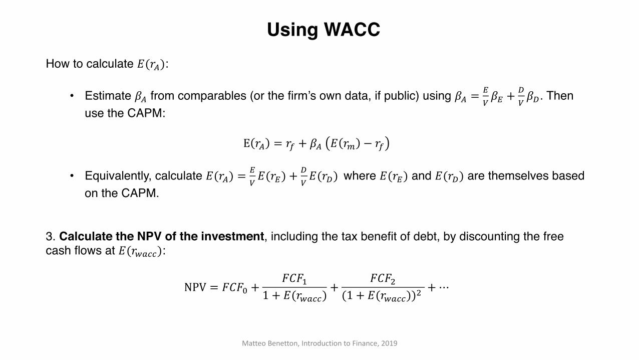
How to calculate !(#$):

• Estimate &$ from comparables (or the firm’s own data, if public) using &$ = () &( +

+) &+. Then

use the CAPM:

E #$ = #- + &$ ! #. − #-

• Equivalently, calculate !(#$) = () !(#() +

+) !(#+) where !(#() and !(#+) are themselves based

on the CAPM.

3. Calculate the NPV of the investment, including the tax benefit of debt, by discounting the free cash flows at !(#0122):

NPV = 6768 +6769

1 + !(#0122)+ 676;(1 + !(#0122));

+ ⋯

Using WACC

Date post:	06-Dec-2021
Category:	Documents
Upload:	others
View:	3 times
Download:	0 times

MBA 203 Executive Summary

Documents