Page 1
7/23/2019 MBA 504 Ch11 Solutions
http://slidepdf.com/reader/full/mba-504-ch11-solutions 1/31
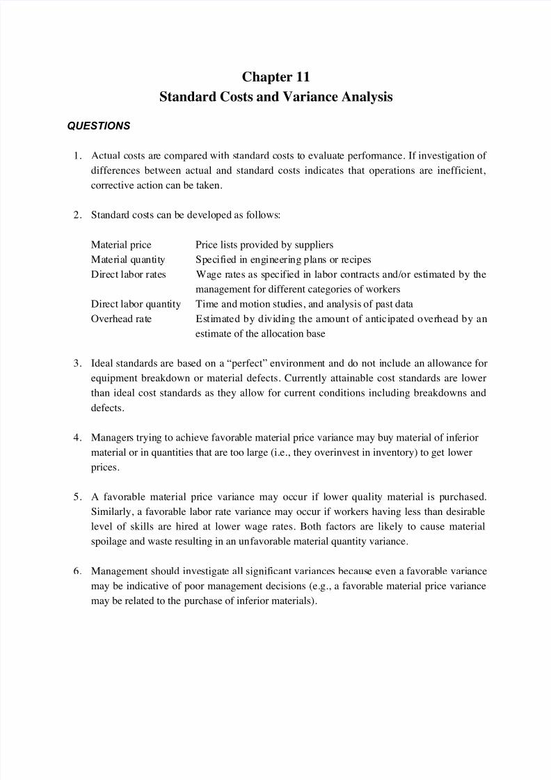
Chapter 11
Standard Costs and Variance Analysis
QUESTIONS
1. Actual costs are compared with standard costs to evaluate performance. If investigation of
differences between actual and standard costs indicates that operations are inefficient,
corrective action can be taken.
2. Standard costs can be developed as follows:
Material price Price lists provided by suppliers
Material quantity Specified in engineering plans or recipes
Direct labor rates Wage rates as specified in labor contracts and/or estimated by themanagement for different categories of workers
Direct labor quantity Time and motion studies, and analysis of past data
Overhead rate Estimated by dividing the amount of anticipated overhead by an
estimate of the allocation base
3. Ideal standards are based on a “perfect” environment and do not include an allowance for
equipment breakdown or material defects. Currently attainable cost standards are lower
than ideal cost standards as they allow for current conditions including breakdowns and
defects.
4. Managers trying to achieve favorable material price variance may buy material of inferior
material or in quantities that are too large (i.e., they overinvest in inventory) to get lower
prices.
5. A favorable material price variance may occur if lower quality material is purchased.
Similarly, a favorable labor rate variance may occur if workers having less than desirable
level of skills are hired at lower wage rates. Both factors are likely to cause material
spoilage and waste resulting in an unfavorable material quantity variance.
6. Management should investigate all significant variances because even a favorable variance
may be indicative of poor management decisions (e.g., a favorable material price variance
may be related to the purchase of inferior materials).
Page 2
7/23/2019 MBA 504 Ch11 Solutions
http://slidepdf.com/reader/full/mba-504-ch11-solutions 2/31
Jiambalvo Managerial Accounting11-2
7. Yes—if total output is less than the output expected at the time the overhead rate was
determined, less fixed overhead will be applied to production compared to the budget (i.e.,
there will be an unfavorable overhead volume variance). This does not indicate that
overhead costs are in or out of control—it simply indicates that production is less than
planned.
8. Only those variances that are deemed exceptional should be investigated. The cost and
likely benefits of variance investigation should be considered in this decision.
9. Management by exception means that special attention is paid to those occurrences (such as
variances) which are deemed exceptional (i.e., out of the ordinary.)
10. It implies that managers should be held accountable for only those variances that they can
control.
11. Variance accounts can be closed by a corresponding debit or credit to either (a) Cost of
Goods Sold only, or (b) proportionately to Work in Process, Finished Goods, and Cost of
Goods Sold.
Page 3
7/23/2019 MBA 504 Ch11 Solutions
http://slidepdf.com/reader/full/mba-504-ch11-solutions 3/31
Chapter 11 Standard Costs and Variance Analysis 11-3
EXERCISES
E1. Unless the Cutting Department reduces production to 500 units per hour,
excess Work in Process Inventory will build up in front of the Chemical Bath
Department. An investment in the excess Work in Process does not createshareholder value.
However, if the Cutting Department reduces production but does not reduce
its work force (hoping that the bottleneck will be eliminated in the near
future), it will have an unfavorable labor efficiency variance. The variance
formula is (AH – SH) SR. Actual hours will not change but standard hours
will be for 500 units, not 600.
E2. If the production process is improved, the standard hours for the quantity
produced may be decreased (it takes less time to produce an item). Now,
unless the work force is reduced or the work force has more items to work on,
an unfavorable labor efficiency variance will result (actual labor hours will be
greater than standard hours).
E3. a. According to the Web site, “Simply put, production variances in SAP are
warning flags that one or more of your standard costs are not right, ‘right’being defined as equal to actual costs.”
b. “The question to ask whenever dollars appear in the Price Variance
account is: Should I adjust my standard cost to be more in line with reality,
or is this a one-time event that will not repeat itself?”
Page 4
7/23/2019 MBA 504 Ch11 Solutions
http://slidepdf.com/reader/full/mba-504-ch11-solutions 4/31
Jiambalvo Managerial Accounting11-4
E4. Material Price Variance
= (AP - SP) AQP
= ($26 - $25) 100
= $100 unfavorable
Actual price = $2,600 ÷ 100 = $26
Material Quantity Variance
= (AQU - SQ) SP
= (83 - 80) $25
= $75 unfavorable
Standard quantity = 40 × 2 = 80
E5. Labor Rate Variance
= (AR - SR) AH
= ($26 - $25) 820
= $820 unfavorable
Actual wage rate = $21,320 ÷ 820 = $26
Labor Efficiency Variance
= (AH - SH) SR
= (820 - 800) $25
= $500 unfavorable
Standard hours = 40 × 20 = 800
Page 5
7/23/2019 MBA 504 Ch11 Solutions
http://slidepdf.com/reader/full/mba-504-ch11-solutions 5/31
Chapter 11 Standard Costs and Variance Analysis 11-5
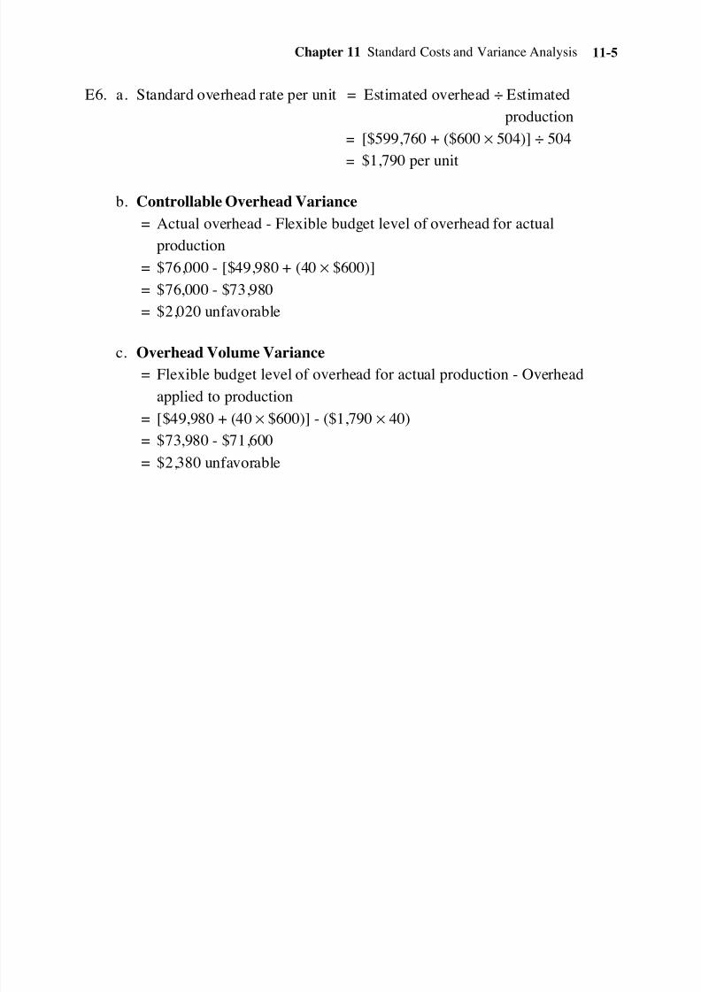
E6. a. Standard overhead rate per unit = Estimated overhead ÷ Estimated
production
= [$599,760 + ($600 × 504)] ÷ 504
= $1,790 per unit
b. Controllable Overhead Variance
= Actual overhead - Flexible budget level of overhead for actual
production
= $76,000 - [$49,980 + (40 × $600)]
= $76,000 - $73,980
= $2,020 unfavorable
c. Overhead Volume Variance
= Flexible budget level of overhead for actual production - Overhead
applied to production
= [$49,980 + (40 × $600)] - ($1,790 × 40)
= $73,980 - $71,600
= $2,380 unfavorable
Page 6
7/23/2019 MBA 504 Ch11 Solutions
http://slidepdf.com/reader/full/mba-504-ch11-solutions 6/31
Jiambalvo Managerial Accounting11-6
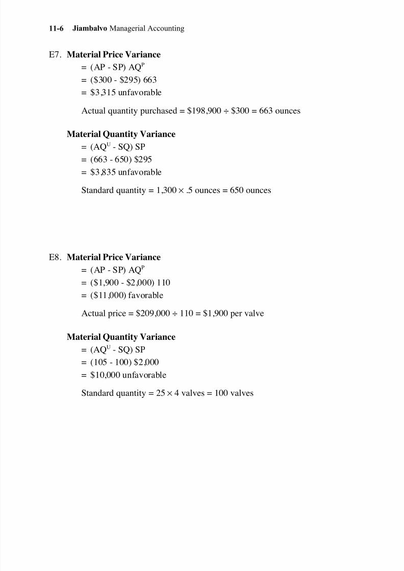
E7. Material Price Variance
= (AP - SP) AQP
= ($300 - $295) 663
= $3,315 unfavorable
Actual quantity purchased = $198,900 ÷ $300 = 663 ounces
Material Quantity Variance
= (AQU - SQ) SP
= (663 - 650) $295
= $3,835 unfavorable
Standard quantity = 1,300 × .5 ounces = 650 ounces
E8. Material Price Variance
= (AP - SP) AQP
= ($1,900 - $2,000) 110
= ($11,000) favorable
Actual price = $209,000 ÷ 110 = $1,900 per valve
Material Quantity Variance
= (AQU - SQ) SP
= (105 - 100) $2,000
= $10,000 unfavorable
Standard quantity = 25 × 4 valves = 100 valves
Page 7
7/23/2019 MBA 504 Ch11 Solutions
http://slidepdf.com/reader/full/mba-504-ch11-solutions 7/31
Chapter 11 Standard Costs and Variance Analysis 11-7
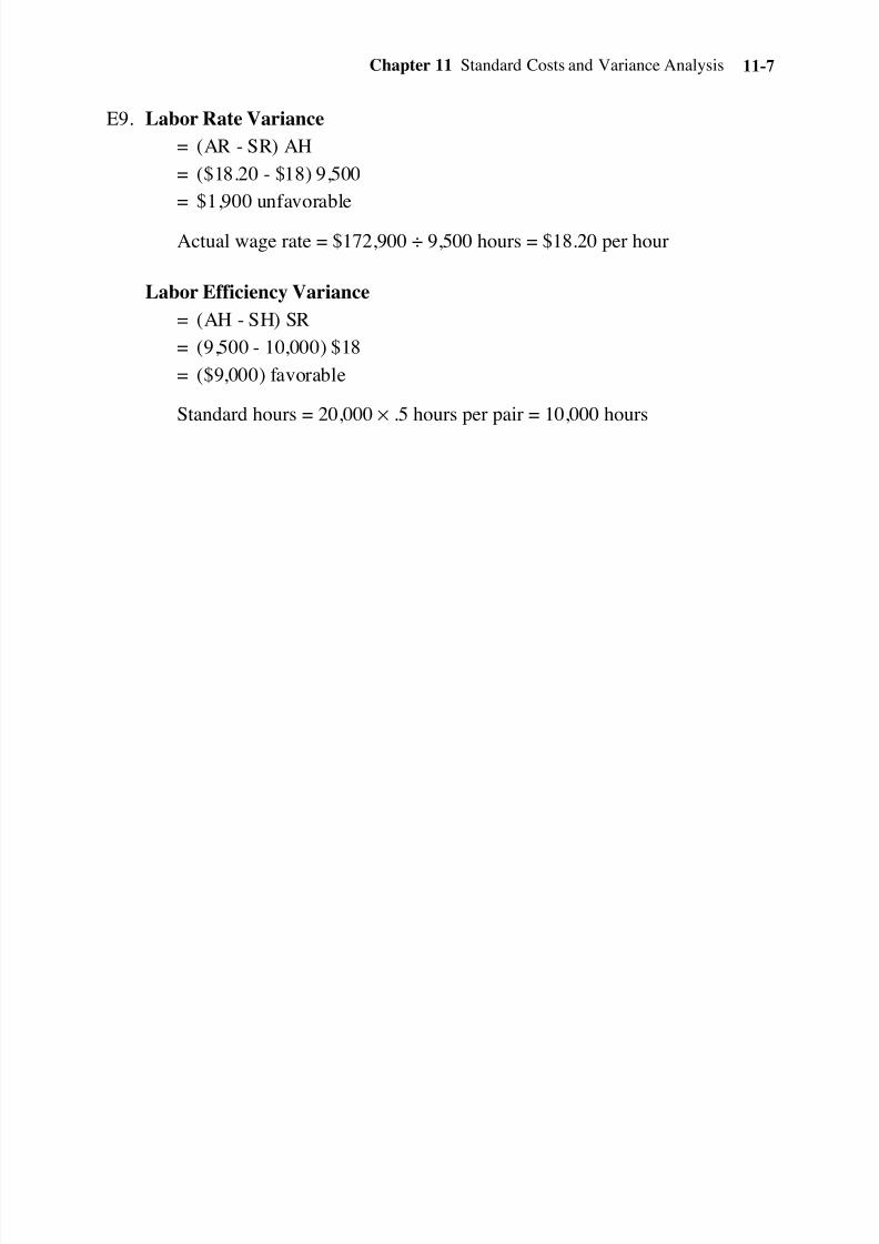
E9. Labor Rate Variance
= (AR - SR) AH
= ($18.20 - $18) 9,500
= $1,900 unfavorable
Actual wage rate = $172,900 ÷ 9,500 hours = $18.20 per hour
Labor Efficiency Variance
= (AH - SH) SR
= (9,500 - 10,000) $18
= ($9,000) favorable
Standard hours = 20,000 × .5 hours per pair = 10,000 hours
Page 8
7/23/2019 MBA 504 Ch11 Solutions
http://slidepdf.com/reader/full/mba-504-ch11-solutions 8/31
Jiambalvo Managerial Accounting11-8
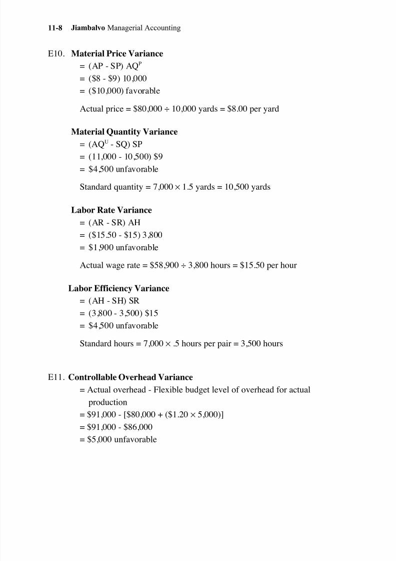
E10. Material Price Variance
= (AP - SP) AQP
= ($8 - $9) 10,000
= ($10,000) favorable
Actual price = $80,000 ÷ 10,000 yards = $8.00 per yard
Material Quantity Variance
= (AQU - SQ) SP
= (11,000 - 10,500) $9
= $4,500 unfavorable
Standard quantity = 7,000 × 1.5 yards = 10,500 yards
Labor Rate Variance
= (AR - SR) AH
= ($15.50 - $15) 3,800
= $1,900 unfavorable
Actual wage rate = $58,900 ÷ 3,800 hours = $15.50 per hour
Labor Efficiency Variance
= (AH - SH) SR
= (3,800 - 3,500) $15
= $4,500 unfavorable
Standard hours = 7,000 × .5 hours per pair = 3,500 hours
E11. Controllable Overhead Variance
= Actual overhead - Flexible budget level of overhead for actualproduction
= $91,000 - [$80,000 + ($1.20 × 5,000)]
= $91,000 - $86,000
= $5,000 unfavorable
Page 9
7/23/2019 MBA 504 Ch11 Solutions
http://slidepdf.com/reader/full/mba-504-ch11-solutions 9/31
Chapter 11 Standard Costs and Variance Analysis 11-9
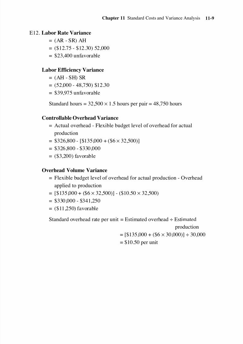
E12. Labor Rate Variance
= (AR - SR) AH
= ($12.75 - $12.30) 52,000
= $23,400 unfavorable
Labor Efficiency Variance
= (AH - SH) SR
= (52,000 - 48,750) $12.30
= $39,975 unfavorable
Standard hours = 32,500 × 1.5 hours per pair = 48,750 hours
Controllable Overhead Variance= Actual overhead - Flexible budget level of overhead for actual
production
= $326,800 - [$135,000 + ($6 × 32,500)]
= $326,800 - $330,000
= ($3,200) favorable
Overhead Volume Variance
= Flexible budget level of overhead for actual production - Overhead
applied to production
= [$135,000 + ($6 × 32,500)] - ($10.50 × 32,500)
= $330,000 - $341,250
= ($11,250) favorable
Standard overhead rate per unit = Estimated overhead ÷ Estimated
production
= [$135,000 + ($6 × 30,000)] ÷ 30,000
= $10.50 per unit
Page 10
7/23/2019 MBA 504 Ch11 Solutions
http://slidepdf.com/reader/full/mba-504-ch11-solutions 10/31
Jiambalvo Managerial Accounting11-10
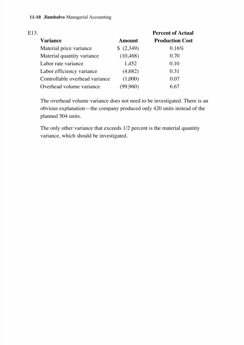
E13. Percent of Actual
Variance Amount Production Cost
Material price variance $ (2,349) 0.16%
Material quantity variance (10,468) 0.70
Labor rate variance 1,452 0.10
Labor efficiency variance (4,682) 0.31
Controllable overhead variance (1,000) 0.07
Overhead volume variance (99,960) 6.67
The overhead volume variance does not need to be investigated. There is an
obvious explanation—the company produced only 420 units instead of the
planned 504 units.
The only other variance that exceeds 1/2 percent is the material quantity
variance, which should be investigated.
Page 11
7/23/2019 MBA 504 Ch11 Solutions
http://slidepdf.com/reader/full/mba-504-ch11-solutions 11/31
Chapter 11 Standard Costs and Variance Analysis 11-11
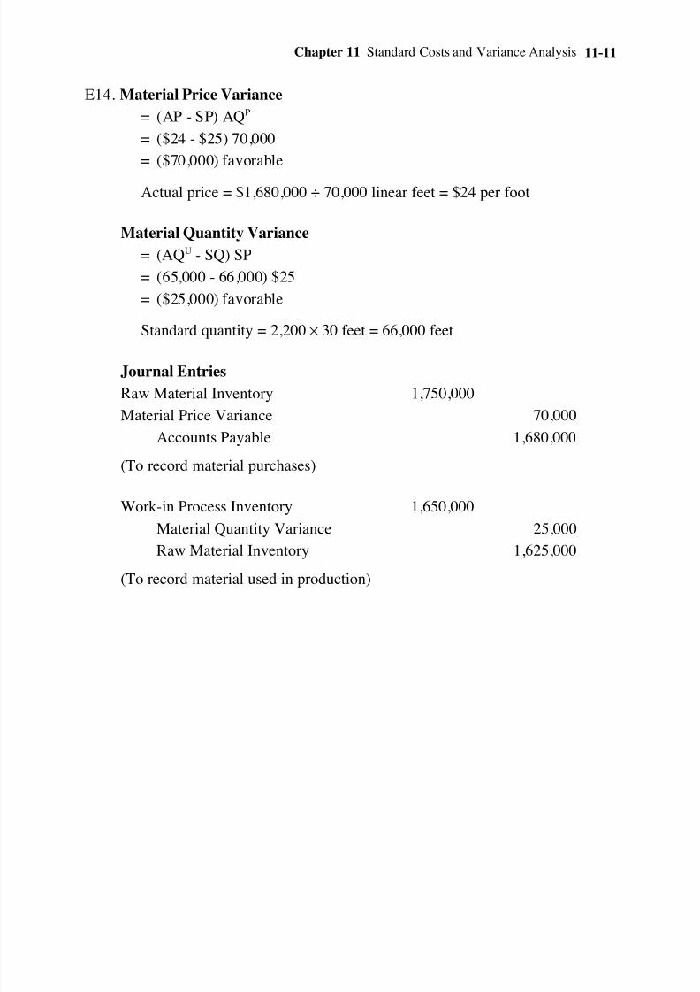
E14. Material Price Variance
= (AP - SP) AQP
= ($24 - $25) 70,000
= ($70,000) favorable
Actual price = $1,680,000 ÷ 70,000 linear feet = $24 per foot
Material Quantity Variance
= (AQU - SQ) SP
= (65,000 - 66,000) $25
= ($25,000) favorable
Standard quantity = 2,200 × 30 feet = 66,000 feet
Journal Entries
Raw Material Inventory 1,750,000
Material Price Variance 70,000
Accounts Payable 1,680,000
(To record material purchases)
Work-in Process Inventory 1,650,000
Material Quantity Variance 25,000
Raw Material Inventory 1,625,000
(To record material used in production)
Page 12
7/23/2019 MBA 504 Ch11 Solutions
http://slidepdf.com/reader/full/mba-504-ch11-solutions 12/31
Jiambalvo Managerial Accounting11-12
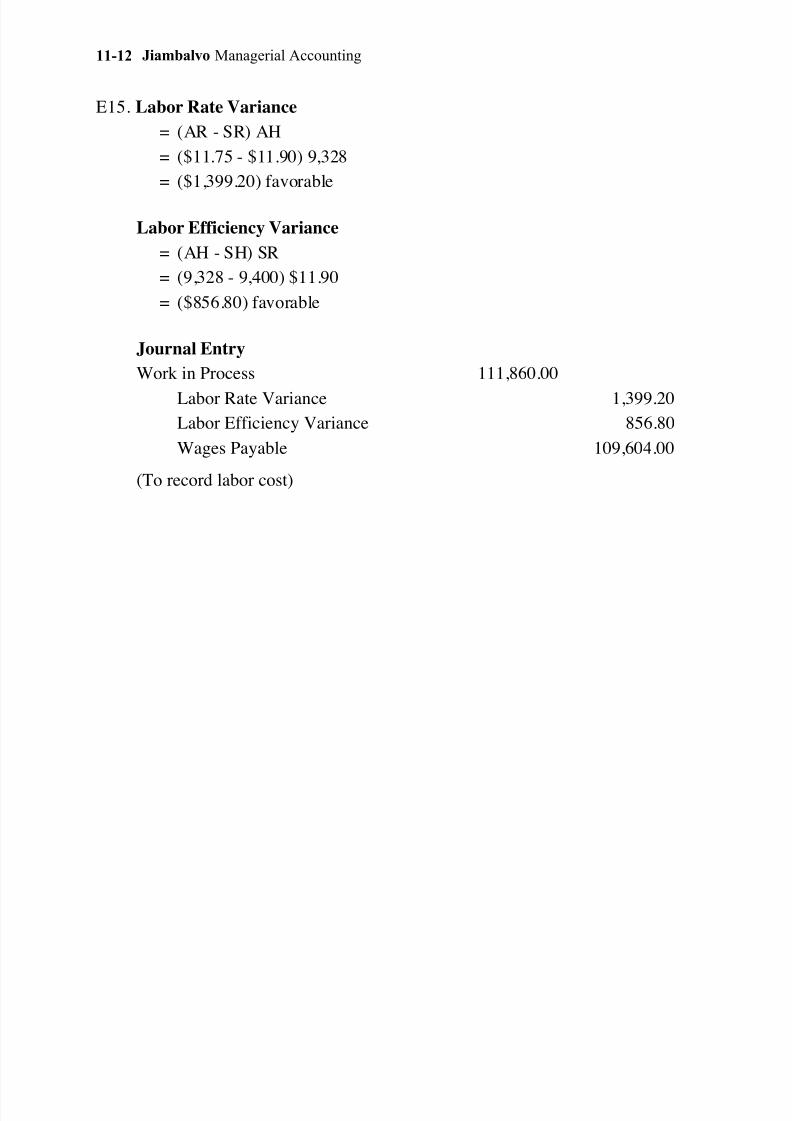
E15. Labor Rate Variance
= (AR - SR) AH
= ($11.75 - $11.90) 9,328
= ($1,399.20) favorable
Labor Efficiency Variance
= (AH - SH) SR
= (9,328 - 9,400) $11.90
= ($856.80) favorable
Journal Entry
Work in Process 111,860.00
Labor Rate Variance 1,399.20
Labor Efficiency Variance 856.80
Wages Payable 109,604.00
(To record labor cost)
Page 13
7/23/2019 MBA 504 Ch11 Solutions
http://slidepdf.com/reader/full/mba-504-ch11-solutions 13/31
Chapter 11 Standard Costs and Variance Analysis 11-13
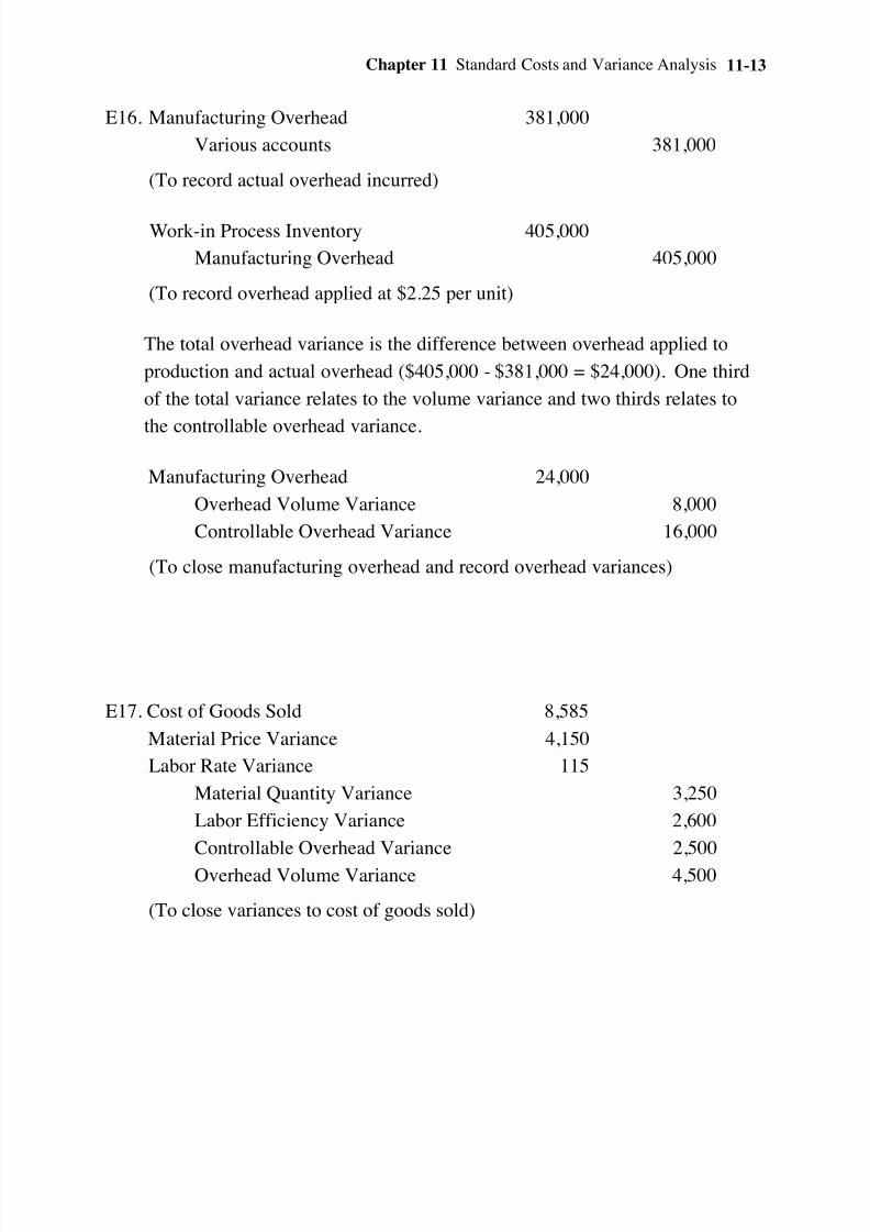
E16. Manufacturing Overhead 381,000
Various accounts 381,000
(To record actual overhead incurred)
Work-in Process Inventory 405,000
Manufacturing Overhead 405,000
(To record overhead applied at $2.25 per unit)
The total overhead variance is the difference between overhead applied to
production and actual overhead ($405,000 - $381,000 = $24,000). One third
of the total variance relates to the volume variance and two thirds relates to
the controllable overhead variance.
Manufacturing Overhead 24,000
Overhead Volume Variance 8,000
Controllable Overhead Variance 16,000
(To close manufacturing overhead and record overhead variances)
E17. Cost of Goods Sold 8,585
Material Price Variance 4,150
Labor Rate Variance 115
Material Quantity Variance 3,250
Labor Efficiency Variance 2,600
Controllable Overhead Variance 2,500
Overhead Volume Variance 4,500
(To close variances to cost of goods sold)
Page 14
7/23/2019 MBA 504 Ch11 Solutions
http://slidepdf.com/reader/full/mba-504-ch11-solutions 14/31
Jiambalvo Managerial Accounting11-14
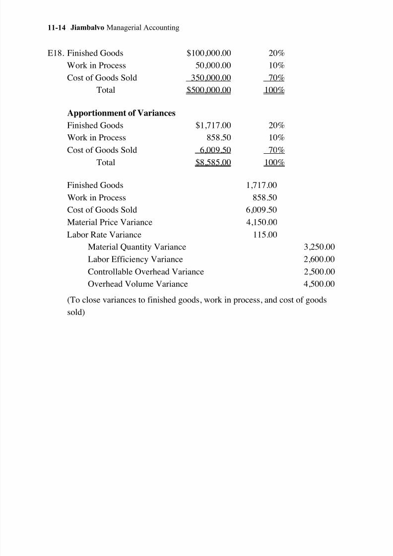
E18. Finished Goods $100,000.00 20%
Work in Process 50,000.00 10%
Cost of Goods Sold 350,000.00 70%
Total $500,000.00 100%
Apportionment of Variances
Finished Goods $1,717.00 20%
Work in Process 858.50 10%
Cost of Goods Sold 6,009.50 70%
Total $8,585.00 100%
Finished Goods 1,717.00
Work in Process 858.50
Cost of Goods Sold 6,009.50
Material Price Variance 4,150.00
Labor Rate Variance 115.00
Material Quantity Variance 3,250.00
Labor Efficiency Variance 2,600.00
Controllable Overhead Variance 2,500.00
Overhead Volume Variance 4,500.00
(To close variances to finished goods, work in process, and cost of goods
sold)
Page 15
7/23/2019 MBA 504 Ch11 Solutions
http://slidepdf.com/reader/full/mba-504-ch11-solutions 15/31
Chapter 11 Standard Costs and Variance Analysis 11-15
PROBLEMS
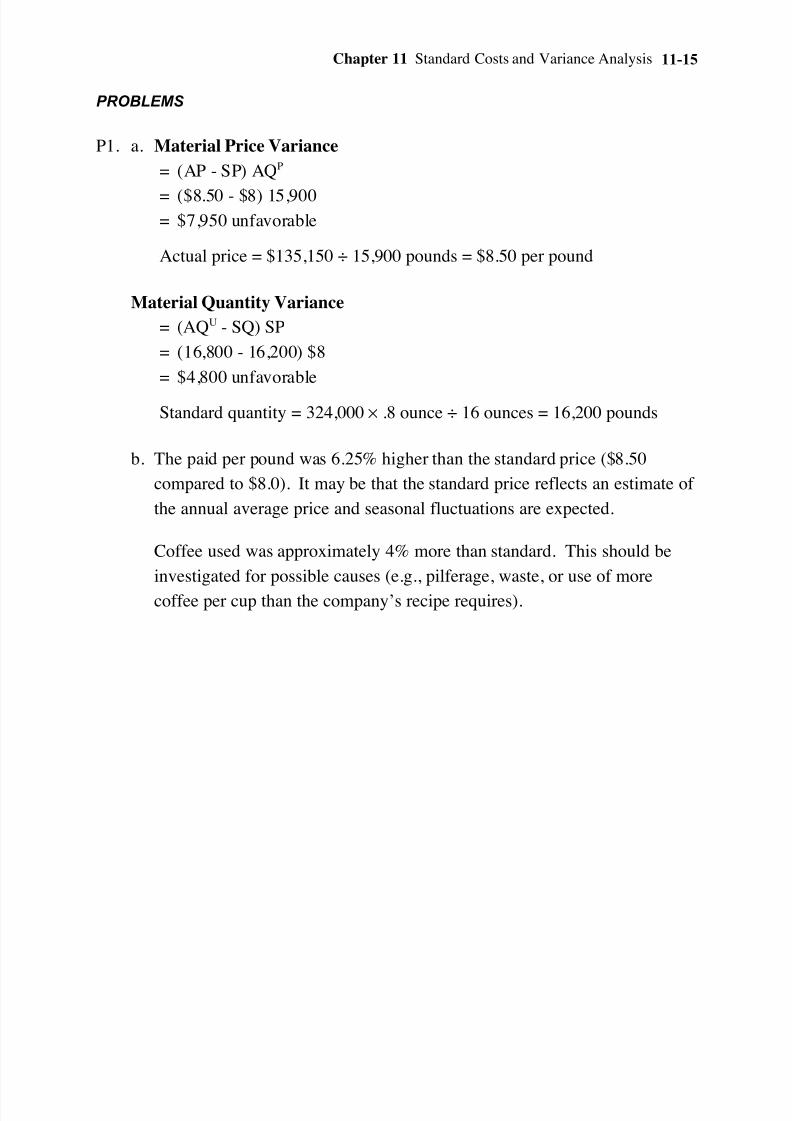
P1. a. Material Price Variance
= (AP - SP) AQP
= ($8.50 - $8) 15,900= $7,950 unfavorable
Actual price = $135,150 ÷ 15,900 pounds = $8.50 per pound
Material Quantity Variance
= (AQU - SQ) SP
= (16,800 - 16,200) $8
= $4,800 unfavorable
Standard quantity = 324,000 × .8 ounce ÷ 16 ounces = 16,200 pounds
b. The paid per pound was 6.25% higher than the standard price ($8.50
compared to $8.0). It may be that the standard price reflects an estimate of
the annual average price and seasonal fluctuations are expected.
Coffee used was approximately 4% more than standard. This should be
investigated for possible causes (e.g., pilferage, waste, or use of more
coffee per cup than the company’s recipe requires).
Page 16
7/23/2019 MBA 504 Ch11 Solutions
http://slidepdf.com/reader/full/mba-504-ch11-solutions 16/31
Jiambalvo Managerial Accounting11-16
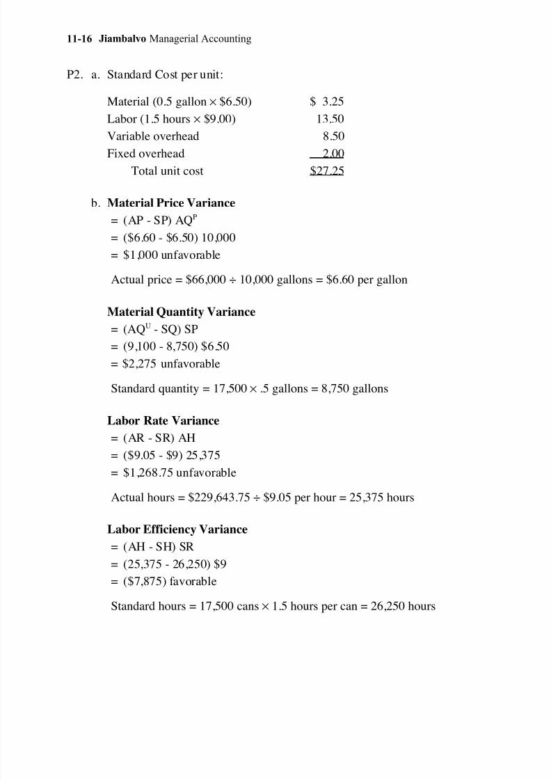
P2. a. Standard Cost per unit:
Material (0.5 gallon × $6.50) $ 3.25
Labor (1.5 hours × $9.00) 13.50
Variable overhead 8.50Fixed overhead 2.00
Total unit cost $27.25
b. Material Price Variance
= (AP - SP) AQP
= ($6.60 - $6.50) 10,000
= $1,000 unfavorable
Actual price = $66,000 ÷ 10,000 gallons = $6.60 per gallon
Material Quantity Variance
= (AQU - SQ) SP
= (9,100 - 8,750) $6.50
= $2,275 unfavorable
Standard quantity = 17,500 × .5 gallons = 8,750 gallons
Labor Rate Variance
= (AR - SR) AH
= ($9.05 - $9) 25,375
= $1,268.75 unfavorable
Actual hours = $229,643.75 ÷ $9.05 per hour = 25,375 hours
Labor Efficiency Variance
= (AH - SH) SR= (25,375 - 26,250) $9
= ($7,875) favorable
Standard hours = 17,500 cans × 1.5 hours per can = 26,250 hours
Page 17
7/23/2019 MBA 504 Ch11 Solutions
http://slidepdf.com/reader/full/mba-504-ch11-solutions 17/31
Chapter 11 Standard Costs and Variance Analysis 11-17
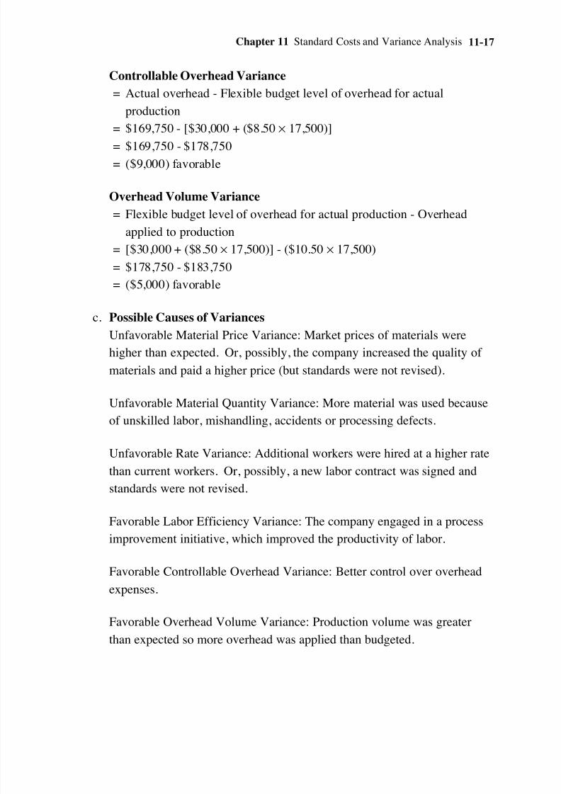
Controllable Overhead Variance
= Actual overhead - Flexible budget level of overhead for actual
production
= $169,750 - [$30,000 + ($8.50 × 17,500)]
= $169,750 - $178,750
= ($9,000) favorable
Overhead Volume Variance
= Flexible budget level of overhead for actual production - Overhead
applied to production
= [$30,000 + ($8.50 × 17,500)] - ($10.50 × 17,500)
= $178,750 - $183,750
= ($5,000) favorable
c. Possible Causes of Variances
Unfavorable Material Price Variance: Market prices of materials were
higher than expected. Or, possibly, the company increased the quality of
materials and paid a higher price (but standards were not revised).
Unfavorable Material Quantity Variance: More material was used because
of unskilled labor, mishandling, accidents or processing defects.
Unfavorable Rate Variance: Additional workers were hired at a higher rate
than current workers. Or, possibly, a new labor contract was signed and
standards were not revised.
Favorable Labor Efficiency Variance: The company engaged in a process
improvement initiative, which improved the productivity of labor.
Favorable Controllable Overhead Variance: Better control over overhead
expenses.
Favorable Overhead Volume Variance: Production volume was greater
than expected so more overhead was applied than budgeted.
Page 18
7/23/2019 MBA 504 Ch11 Solutions
http://slidepdf.com/reader/full/mba-504-ch11-solutions 18/31
Jiambalvo Managerial Accounting11-18
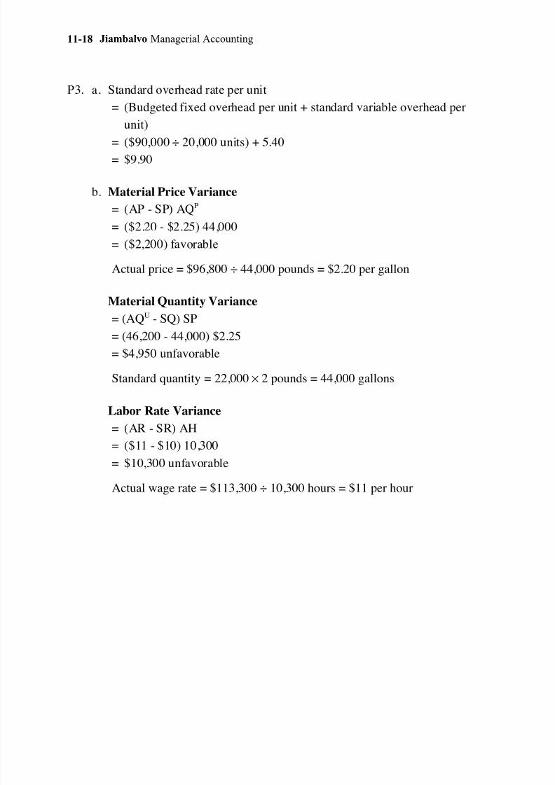
P3. a. Standard overhead rate per unit
= (Budgeted fixed overhead per unit + standard variable overhead per
unit)
= ($90,000 ÷ 20,000 units) + 5.40
= $9.90
b. Material Price Variance
= (AP - SP) AQP
= ($2.20 - $2.25) 44,000
= ($2,200) favorable
Actual price = $96,800 ÷ 44,000 pounds = $2.20 per gallon
Material Quantity Variance
= (AQU - SQ) SP
= (46,200 - 44,000) $2.25
= $4,950 unfavorable
Standard quantity = 22,000 × 2 pounds = 44,000 gallons
Labor Rate Variance= (AR - SR) AH
= ($11 - $10) 10,300
= $10,300 unfavorable
Actual wage rate = $113,300 ÷ 10,300 hours = $11 per hour
Page 19
7/23/2019 MBA 504 Ch11 Solutions
http://slidepdf.com/reader/full/mba-504-ch11-solutions 19/31
Chapter 11 Standard Costs and Variance Analysis 11-19
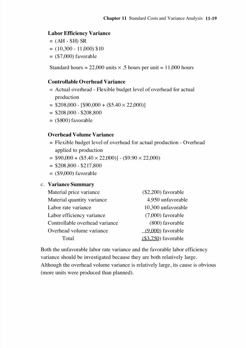
Labor Efficiency Variance
= (AH - SH) SR
= (10,300 - 11,000) $10
= ($7,000) favorable
Standard hours = 22,000 units × .5 hours per unit = 11,000 hours
Controllable Overhead Variance
= Actual overhead - Flexible budget level of overhead for actual
production
= $208,000 - [$90,000 + ($5.40 × 22,000)]
= $208,000 - $208,800
= ($800) favorable
Overhead Volume Variance
= Flexible budget level of overhead for actual production - Overhead
applied to production
= $90,000 + ($5.40 × 22,000)] - ($9.90 × 22,000)
= $208,800 - $217,800
= ($9,000) favorable
c. Variance Summary
Material price variance ($2,200) favorable
Material quantity variance 4,950 unfavorable
Labor rate variance 10,300 unfavorable
Labor efficiency variance (7,000) favorable
Controllable overhead variance (800) favorable
Overhead volume variance (9,000) favorable
Total ($3,750) favorable
Both the unfavorable labor rate variance and the favorable labor efficiency
variance should be investigated because they are both relatively large.
Although the overhead volume variance is relatively large, its cause is obvious
(more units were produced than planned).
Page 20
7/23/2019 MBA 504 Ch11 Solutions
http://slidepdf.com/reader/full/mba-504-ch11-solutions 20/31
Jiambalvo Managerial Accounting11-20
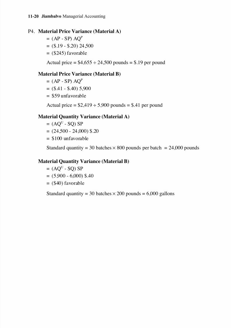
P4. Material Price Variance (Material A)
= (AP - SP) AQP
= ($.19 - $.20) 24,500
= ($245) favorable
Actual price = $4,655 ÷ 24,500 pounds = $.19 per pound
Material Price Variance (Material B)
= (AP - SP) AQP
= ($.41 - $.40) 5,900
= $59 unfavorable
Actual price = $2,419 ÷ 5,900 pounds = $.41 per pound
Material Quantity Variance (Material A)
= (AQU - SQ) SP
= (24,500 - 24,000) $.20
= $100 unfavorable
Standard quantity = 30 batches × 800 pounds per batch = 24,000 pounds
Material Quantity Variance (Material B)
= (AQU - SQ) SP
= (5,900 - 6,000) $.40
= ($40) favorable
Standard quantity = 30 batches × 200 pounds = 6,000 gallons
Page 21
7/23/2019 MBA 504 Ch11 Solutions
http://slidepdf.com/reader/full/mba-504-ch11-solutions 21/31
Chapter 11 Standard Costs and Variance Analysis 11-21
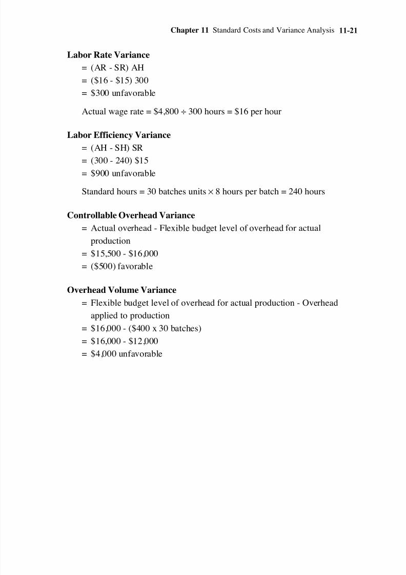
Labor Rate Variance
= (AR - SR) AH
= ($16 - $15) 300
= $300 unfavorable
Actual wage rate = $4,800 ÷ 300 hours = $16 per hour
Labor Efficiency Variance
= (AH - SH) SR
= (300 - 240) $15
= $900 unfavorable
Standard hours = 30 batches units × 8 hours per batch = 240 hours
Controllable Overhead Variance
= Actual overhead - Flexible budget level of overhead for actual
production
= $15,500 - $16,000
= ($500) favorable
Overhead Volume Variance
= Flexible budget level of overhead for actual production - Overheadapplied to production
= $16,000 - ($400 x 30 batches)
= $16,000 - $12,000
= $4,000 unfavorable
Page 22
7/23/2019 MBA 504 Ch11 Solutions
http://slidepdf.com/reader/full/mba-504-ch11-solutions 22/31
Jiambalvo Managerial Accounting11-22
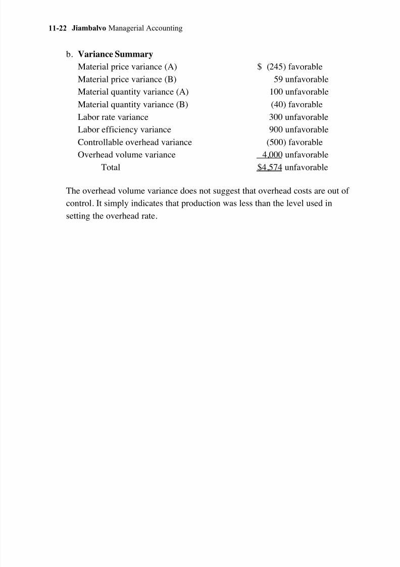
b. Variance Summary
Material price variance (A) $ (245) favorable
Material price variance (B) 59 unfavorable
Material quantity variance (A) 100 unfavorable
Material quantity variance (B) (40) favorable
Labor rate variance 300 unfavorable
Labor efficiency variance 900 unfavorable
Controllable overhead variance (500) favorable
Overhead volume variance 4,000 unfavorable
Total $4,574 unfavorable
The overhead volume variance does not suggest that overhead costs are out of
control. It simply indicates that production was less than the level used in
setting the overhead rate.
Page 23
7/23/2019 MBA 504 Ch11 Solutions
http://slidepdf.com/reader/full/mba-504-ch11-solutions 23/31
Chapter 11 Standard Costs and Variance Analysis 11-23
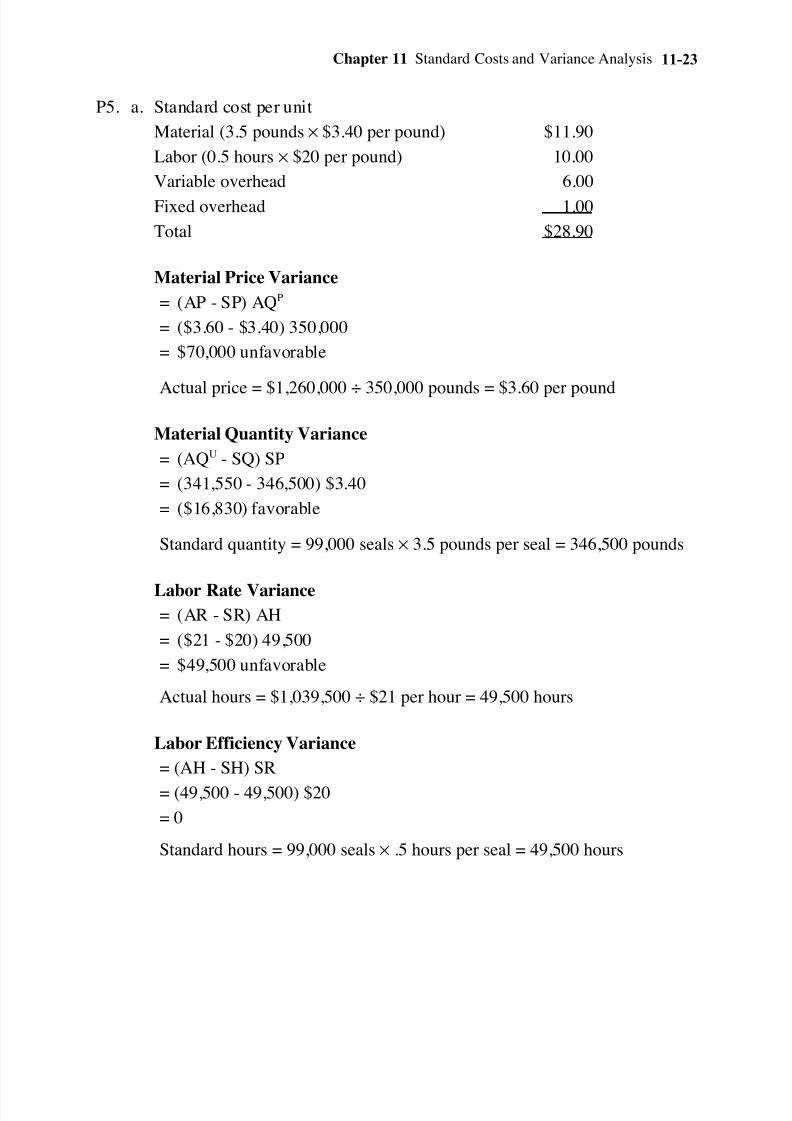
P5. a. Standard cost per unit
Material (3.5 pounds × $3.40 per pound) $11.90
Labor (0.5 hours × $20 per pound) 10.00
Variable overhead 6.00
Fixed overhead 1.00
Total $28.90
Material Price Variance
= (AP - SP) AQP
= ($3.60 - $3.40) 350,000
= $70,000 unfavorable
Actual price = $1,260,000 ÷ 350,000 pounds = $3.60 per pound
Material Quantity Variance
= (AQU - SQ) SP
= (341,550 - 346,500) $3.40
= ($16,830) favorable
Standard quantity = 99,000 seals × 3.5 pounds per seal = 346,500 pounds
Labor Rate Variance= (AR - SR) AH
= ($21 - $20) 49,500
= $49,500 unfavorable
Actual hours = $1,039,500 ÷ $21 per hour = 49,500 hours
Labor Efficiency Variance
= (AH - SH) SR
= (49,500 - 49,500) $20
= 0
Standard hours = 99,000 seals × .5 hours per seal = 49,500 hours
Page 24
7/23/2019 MBA 504 Ch11 Solutions
http://slidepdf.com/reader/full/mba-504-ch11-solutions 24/31
Jiambalvo Managerial Accounting11-24
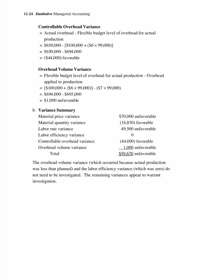
Controllable Overhead Variance
= Actual overhead - Flexible budget level of overhead for actual
production
= $650,000 - [$100,000 + ($6 × 99,000)]
= $650,000 - $694,000
= ($44,000) favorable
Overhead Volume Variance
= Flexible budget level of overhead for actual production - Overhead
applied to production
= [$100,000 + ($6 × 99,000)] - ($7 × 99,000)
= $694,000 - $693,000
= $1,000 unfavorable
b. Variance Summary
Material price variance $70,000 unfavorable
Material quantity variance (16,830) favorable
Labor rate variance 49,500 unfavorable
Labor efficiency variance 0
Controllable overhead variance (44,000) favorable
Overhead volume variance 1,000 unfavorableTotal $59,670 unfavorable
The overhead volume variance (which occurred because actual production
was less than planned) and the labor efficiency variance (which was zero) do
not need to be investigated. The remaining variances appear to warrant
investigation.
Page 25
7/23/2019 MBA 504 Ch11 Solutions
http://slidepdf.com/reader/full/mba-504-ch11-solutions 25/31
Chapter 11 Standard Costs and Variance Analysis 11-25
P6. Labor Rate Variance
= (AR - SR) AH
= ($32.5467 - $25) 322
= $2,430.04 unfavorable
Actual rate = $10,480 ÷ 322 hours = $32.5467 per hour
Labor Efficiency Variance
= (AH - SH) SR
= (322 - 302.4167) $25
= $489.58 unfavorable
Standard hours = 1,910 samples × 9.5 minutes per sample ÷ 60 minutes =
302.4167 hours
Although the labor rate variance is relatively large, its cause is fairly obvious.
It is not surprising that the company would need to pay a relatively high wage
rate to a temporary worker with the skills to draw and prepare blood samples.
As only 322 hours of work were performed in the month, it appears that the
lab had only two full-time employees. Based on $40 per hour for one of them
and $25 per hour for the other, and assuming that each worked an equal
number of hours, the expected total cost at an average rate of $32.50 [($40 +
25) ÷2] is $10,465. With this in mind, the actual cost of $10,480 does not
seem to be out of line.
Page 26
7/23/2019 MBA 504 Ch11 Solutions
http://slidepdf.com/reader/full/mba-504-ch11-solutions 26/31
Jiambalvo Managerial Accounting11-26
P7. a. Will should not act according to his initial instinct—the causes of the
variances should be determined before managers are rewarded/punished.
b. The favorable material price variance could be due to purchasing inferior
materials at a price less than standard. This could lead to material waste,
which would show up in an unfavorable material quantity variance. It
could also lead to an unfavorable labor efficiency variance if workers need
to spend more time (than standard) to produce defect free units.
c. Will should investigate the causes for variances before determining
rewards or punishments.
Page 27
7/23/2019 MBA 504 Ch11 Solutions
http://slidepdf.com/reader/full/mba-504-ch11-solutions 27/31
Chapter 11 Standard Costs and Variance Analysis 11-27
P8. a. No. Fewer customer calls and less time per call could result from bad as
well as good performance.
b. Favorable variance could occur because of good performance if:
(1) Software quality improved so that customers did not need to call
customer support as often, and if they did call, problems were simpler and
could be solved in less time.
(2) Customer support quality improved so that customers did not need to
call repeatedly for the same problem. And, when customers called,
questions were answered correctly and quickly.
Favorable variance could occur because of bad performance if:(1) Software quality deteriorated resulting in much lower sales and,
consequently, fewer customers called (although the remaining customers
made frequent calls).
(2) Customer support quality deteriorated as employees tried to cut-off
customer calls in order to reduce the “time per call” measure, and the
customers were so dissatisfied that they were discouraged from calling.
The scenario is more likely if the software magazine review is reliable.
Page 28
7/23/2019 MBA 504 Ch11 Solutions
http://slidepdf.com/reader/full/mba-504-ch11-solutions 28/31
Jiambalvo Managerial Accounting11-28
P9. a. The favorable material price variance is due to the purchase of inferior
materials at a bargain price. This could lead to an unfavorable material
quantity variance if extra material needed to be used because of material
defects and the need to rework defective products.
The favorable labor rate variance is due to use of temporary replacement
workers who are paid lower wage rates. But the use of replacement
workers will lead to an unfavorable labor efficiency variance if the
replacement workers are not able to produce items as efficiently as
permanent workers.
b. I would not characterize as a good decision the decision to purchase
materials at a bargain price. The materials are inferior and may
compromise product quality, the reputation of the company, andshareholder value.
P10. Due to the strike, 500,000 Road Guardian batteries were not produced and
sold. How did this affect profit? The batteries sell for $30 per unit and the
variable cost (assuming that overhead is essentially fixed due to the high
level of investment in automation) is $5 ($3 of material and $2 of labor).
Thus the contribution margin is $25. The effect of not producing and
selling 500,000 Road Guardians is $12,500,000 ($25 x 500,000).
The controller recognizes that the strike reduced productive capacity.
However, he measures the cost of reduced capacity in terms of the
difference between the amount of overhead in the flexible budget (which
equals the amount in a static budget because all overhead is fixed) and the
amount applied to inventory (a difference of $5,000,000). This difference
is the overhead volume variance. It indicates that $5,000,000 of overhead
was not applied to production, but that is not a reasonable measure of the
effect of the strike. Overhead is essentially fixed and overhead was
actually less than budgeted (by a relatively small amount). The effect of reduced capacity on profit needs to be assessed in terms of the lost
contribution margin related to reduced capacity. As we saw above, the
effect of the strike was reduced production of the Road Guardian by
500,000 units. Since the Road Guardian has a contribution margin of $25,
the impact of the strike was $12,500,000.
Page 29
7/23/2019 MBA 504 Ch11 Solutions
http://slidepdf.com/reader/full/mba-504-ch11-solutions 29/31
Chapter 11 Standard Costs and Variance Analysis 11-29
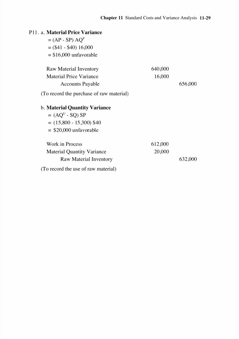
P11. a. Material Price Variance
= (AP - SP) AQP
= ($41 - $40) 16,000
= $16,000 unfavorable
Raw Material Inventory 640,000
Material Price Variance 16,000
Accounts Payable 656,000
(To record the purchase of raw material)
b. Material Quantity Variance
= (AQU - SQ) SP
= (15,800 - 15,300) $40
= $20,000 unfavorable
Work in Process 612,000
Material Quantity Variance 20,000
Raw Material Inventory 632,000
(To record the use of raw material)
Page 30
7/23/2019 MBA 504 Ch11 Solutions
http://slidepdf.com/reader/full/mba-504-ch11-solutions 30/31
Jiambalvo Managerial Accounting11-30
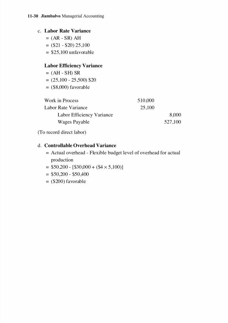
c. Labor Rate Variance
= (AR - SR) AH
= ($21 - $20) 25,100
= $25,100 unfavorable
Labor Efficiency Variance
= (AH - SH) SR
= (25,100 - 25,500) $20
= ($8,000) favorable
Work in Process 510,000
Labor Rate Variance 25,100
Labor Efficiency Variance 8,000
Wages Payable 527,100
(To record direct labor)
d. Controllable Overhead Variance
= Actual overhead - Flexible budget level of overhead for actual
production
= $50,200 - [$30,000 + ($4 × 5,100)]
= $50,200 - $50,400
= ($200) favorable
Page 31
7/23/2019 MBA 504 Ch11 Solutions
http://slidepdf.com/reader/full/mba-504-ch11-solutions 31/31
Chapter 11 Standard Costs and Variance Analysis 11-31
Overhead Volume Variance
= Flexible budget level of overhead for actual production - Overhead
applied to production
= [$30,000 + ($4 × 5,100)] - ($10 × 5,100)
= $50,400 - $51,000
= ($600) favorable
Work in Process 51,000
Manufacturing Overhead 51,000
(To record overhead applied to production)
Manufacturing Overhead 50,200
Various Accounts 50,200
(To record actual overhead)
Manufacturing Overhead 800
Controllable Overhead Variance 200
Overhead Volume Variance 600
(To close Manufacturing Overhead and record overhead variances)
e. Cost of Goods Sold 52,300
Labor Efficiency Variance 8,000
Controllable Overhead Variance 200
Overhead Volume Variance 600
Material Price Variance 16,000
Material Quantity Variance 20,000
Labor Rate Variance 25,100
(To close variance accounts to Cost of Goods Sold)