57
1 Course: MBA Subject: Quantitative Techniques Unit:1.1
| Date post: | 15-Jul-2015 |
| Category: |
Education |
| Upload: | rai-university |
| View: | 195 times |
| Download: | 4 times |
1
Course: MBASubject: Quantitative
TechniquesUnit:1.1
2
• A Linear Programming model seeks to maximize or minimize a linear function, subject to a set of linear constraints.
• The linear model consists of the followingcomponents:– A set of decision variables.– An objective function.– A set of constraints.
2.1 Introduction to Linear Programming2.1 Introduction to Linear Programming

3
Introduction to Linear ProgrammingIntroduction to Linear Programming
• The Importance of Linear Programming– Many real world problems lend themselves to linear programming modeling. – Many real world problems can be approximated by linear models.– There are well-known successful applications in:
• Manufacturing• Marketing• Finance (investment)• Advertising• Agriculture
4
• The Importance of Linear Programming– There are efficient solution techniques that solve linear
programming models.– The output generated from linear programming packages
provides useful “what if” analysis.
Introduction to Linear ProgrammingIntroduction to Linear Programming
5
Introduction to Linear ProgrammingIntroduction to Linear Programming
• Assumptions of the linear programming model– The parameter values are known with certainty.– The objective function and constraints exhibit
constant returns to scale.– There are no interactions between the decision
variables (the additivity assumption).– The Continuity assumption: Variables can take on
any value within a given feasible range.

6
The Galaxy Industries Production Problem – The Galaxy Industries Production Problem – A Prototype ExampleA Prototype Example
• Galaxy manufactures two toy doll models:– Space Ray. – Zapper.
• Resources are limited to– 1000 pounds of special plastic.– 40 hours of production time per week.
7
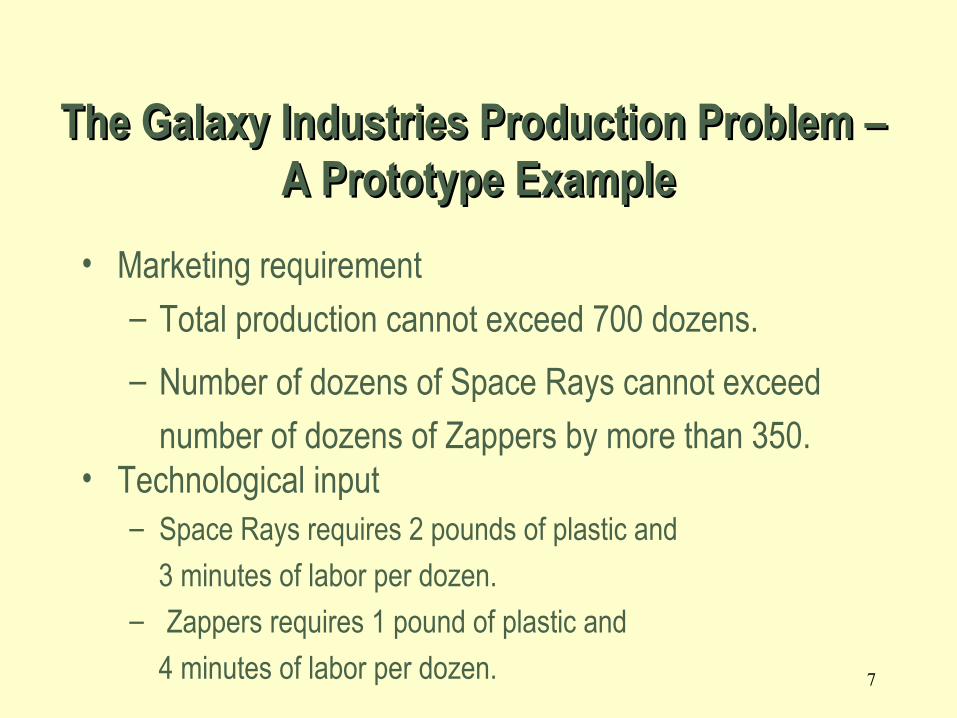
• Marketing requirement– Total production cannot exceed 700 dozens.
– Number of dozens of Space Rays cannot exceed
number of dozens of Zappers by more than 350.• Technological input
– Space Rays requires 2 pounds of plastic and
3 minutes of labor per dozen.– Zappers requires 1 pound of plastic and
4 minutes of labor per dozen.
The Galaxy Industries Production Problem – The Galaxy Industries Production Problem – A Prototype ExampleA Prototype Example
8
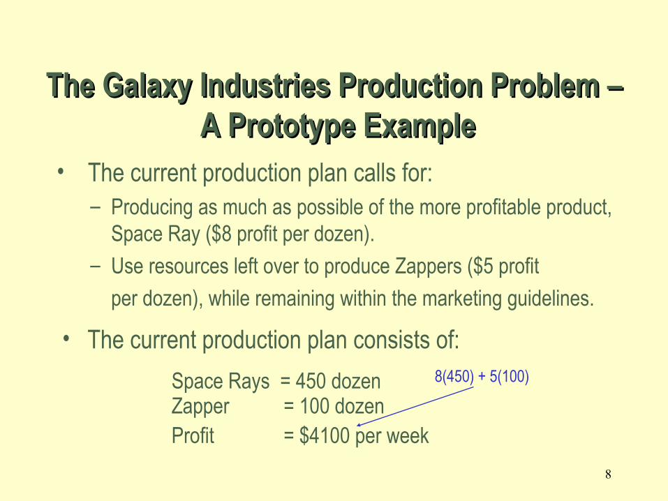
• The current production plan calls for: – Producing as much as possible of the more profitable product,
Space Ray ($8 profit per dozen).– Use resources left over to produce Zappers ($5 profit
per dozen), while remaining within the marketing guidelines.
• The current production plan consists of:
Space Rays = 450 dozenZapper = 100 dozenProfit = $4100 per week
The Galaxy Industries Production Problem –The Galaxy Industries Production Problem – A Prototype Example A Prototype Example
8(450) + 5(100)

9
Management is seeking a production schedule that will increase the company’s profit.

10
A linear programming model can provide an insight and an intelligent solution to this problem.

11
• Decisions variables::
– X1 = Weekly production level of Space Rays (in dozens)
– X2 = Weekly production level of Zappers (in dozens).
• Objective Function:
– Weekly profit, to be maximized
The Galaxy Linear Programming ModelThe Galaxy Linear Programming Model
12
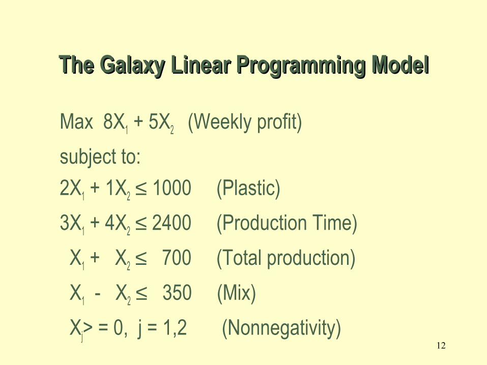
Max 8X1 + 5X2 (Weekly profit)
subject to:
2X1 + 1X2 ≤ 1000 (Plastic)
3X1 + 4X2 ≤ 2400 (Production Time)
X1 + X2 ≤ 700 (Total production)
X1 - X2 ≤ 350 (Mix)
Xj> = 0, j = 1,2 (Nonnegativity)
The Galaxy Linear Programming ModelThe Galaxy Linear Programming Model

13
2.3 2.3 The Graphical Analysis of Linear The Graphical Analysis of Linear ProgrammingProgramming
The set of all points that satisfy all the constraints of the model is called
a
FEASIBLE REGIONFEASIBLE REGION

14
Using a graphical presentation
we can represent all the constraints,
the objective function, and the three
types of feasible points.

15
The non-negativity constraints
X2
X1
Graphical Analysis – the Feasible RegionGraphical Analysis – the Feasible Region
16
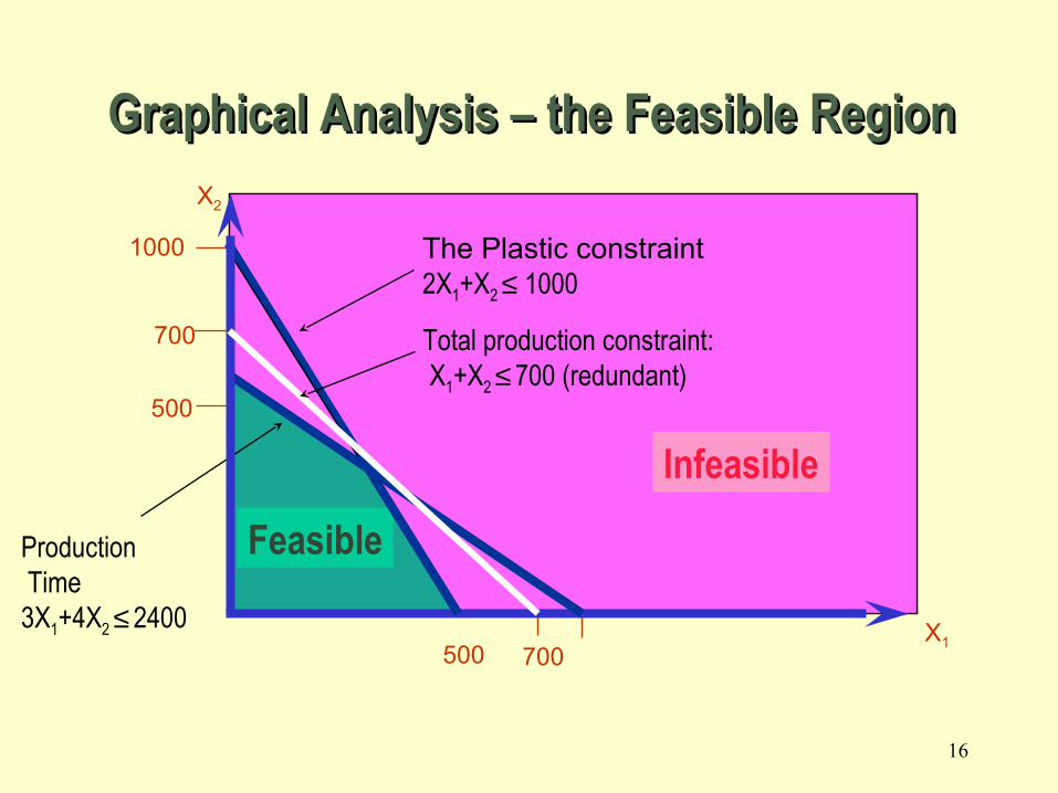
1000
500
Feasible
X2
Infeasible
Production Time3X1+4X2 ≤ 2400
Total production constraint: X1+X2 ≤ 700 (redundant)
500
700
The Plastic constraint2X1+X2 ≤ 1000
X1
700
Graphical Analysis – the Feasible RegionGraphical Analysis – the Feasible Region

17
1000
500
Feasible
X2
Infeasible
Production Time3X1+4X2≤ 2400
Total production constraint: X1+X2 ≤ 700 (redundant)
500
700
Production mix constraint:X1-X2 ≤ 350
The Plastic constraint2X1+X2 ≤ 1000
X1
700
Graphical Analysis – the Feasible RegionGraphical Analysis – the Feasible Region
• There are three types of feasible pointsInterior points. Boundary points. Extreme points.

18
Solving Graphically for an Solving Graphically for an Optimal SolutionOptimal Solution

19
The search for an optimal solutionThe search for an optimal solution
Start at some arbitrary profit, say profit = $2,000...
Then increase the profit, if possible...
...and continue until it becomes infeasible
Profit =$4360
500
700
1000
500
X2
X1
20
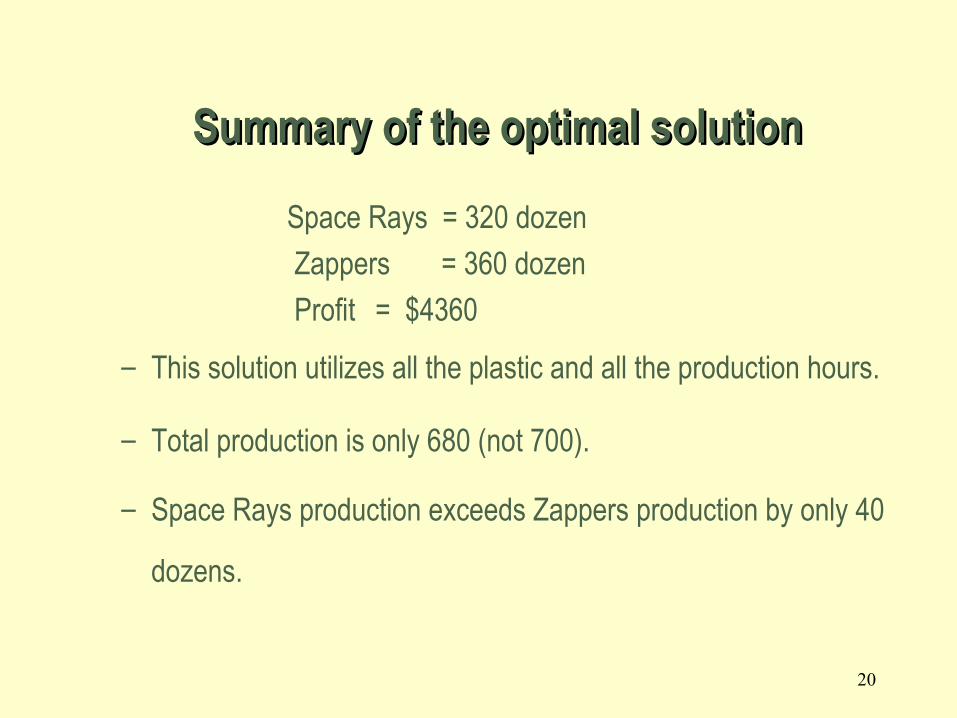
Summary of the optimal solution Summary of the optimal solution
Space Rays = 320 dozen
Zappers = 360 dozen
Profit = $4360
– This solution utilizes all the plastic and all the production hours.
– Total production is only 680 (not 700).
– Space Rays production exceeds Zappers production by only 40
dozens.
21
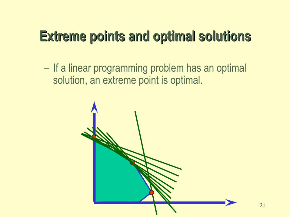
– If a linear programming problem has an optimal solution, an extreme point is optimal.
Extreme points and optimal solutionsExtreme points and optimal solutions

22
• For multiple optimal solutions to exist, the objective function must be parallel to one of the constraints
Multiple optimal solutionsMultiple optimal solutions
•Any weighted average of optimal solutions is also an optimal solution.
23
2.4 The Role of Sensitivity Analysis 2.4 The Role of Sensitivity Analysis of the Optimal Solutionof the Optimal Solution
• Is the optimal solution sensitive to changes in input parameters?
• Possible reasons for asking this question:– Parameter values used were only best estimates.– Dynamic environment may cause changes.– “What-if” analysis may provide economical and
operational information.
24
• Range of Optimality– The optimal solution will remain unchanged as long as
• An objective function coefficient lies within its range of
optimality • There are no changes in any other input parameters.
– The value of the objective function will change if the
coefficient multiplies a variable whose value is nonzero.
Sensitivity Analysis of Sensitivity Analysis of Objective Function Coefficients.Objective Function Coefficients.

25
500
1000
500 800
X2
X1Max 8X
1 + 5X2
Max 4X1 + 5X
2
Max 3.75X1 + 5X
2
Max 2X1 + 5X
2
Sensitivity Analysis of Sensitivity Analysis of Objective Function Coefficients.Objective Function Coefficients.
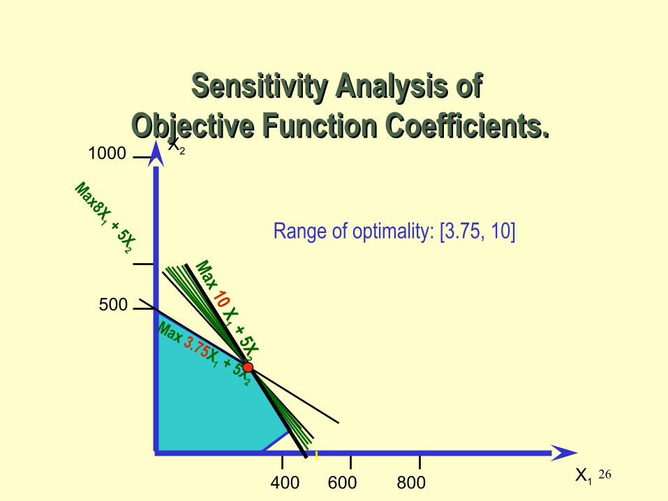
26
500
1000
400 600 800
X2
X1
Max8X1 + 5X
2
Max 3.75X1 + 5X
2
Max 10 X
1 + 5X2
Range of optimality: [3.75, 10]
Sensitivity Analysis of Sensitivity Analysis of Objective Function Coefficients.Objective Function Coefficients.

27
• Reduced costAssuming there are no other changes to the input parameters, the reduced cost for a variable Xj that has a value of “0” at the optimal solution is:
– The negative of the objective coefficient increase of the variable Xj (-∆Cj) necessary for the variable to be positive in the optimal solution
– Alternatively, it is the change in the objective value per unit increase of Xj.
• Complementary slackness At the optimal solution, either the value of a variable is zero, or its reduced cost is 0.
28
• In sensitivity analysis of right-hand sides of constraints we are interested in the following questions:
– Keeping all other factors the same, how much would the optimal value of the objective function (for example, the profit) change if the right-hand side of a constraint changed by one unit?
– For how many additional or fewer units will this per unit change be valid?
Sensitivity Analysis of Sensitivity Analysis of Right-Hand Side ValuesRight-Hand Side Values
29
• Any change to the right hand side of a binding constraint will change the optimal solution.
• Any change to the right-hand side of a non-binding constraint that is less than its slack or surplus, will cause no change in the optimal solution.
Sensitivity Analysis of Sensitivity Analysis of Right-Hand Side ValuesRight-Hand Side Values

30
Shadow PricesShadow Prices
• Assuming there are no other changes to the input parameters, the change to the objective function value per unit increase to a right hand side of a constraint is called the “Shadow Price”
31
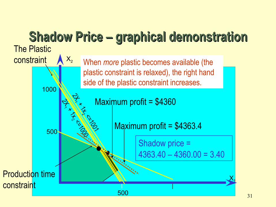
1000
500
X2
X1
500
2X1 + 1x
2 <=1000
When more plastic becomes available (the plastic constraint is relaxed), the right hand side of the plastic constraint increases.
Production timeconstraint
Maximum profit = $4360
2X1 + 1x
2 <=1001 Maximum profit = $4363.4
Shadow price = 4363.40 – 4360.00 = 3.40
Shadow Price – graphical demonstrationShadow Price – graphical demonstrationThe Plastic constraint
32
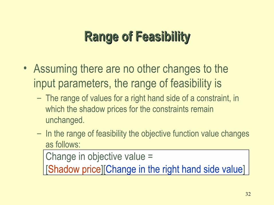
Range of FeasibilityRange of Feasibility
• Assuming there are no other changes to the input parameters, the range of feasibility is– The range of values for a right hand side of a constraint, in
which the shadow prices for the constraints remain unchanged.
– In the range of feasibility the objective function value changes as follows:Change in objective value = [Shadow price][Change in the right hand side value]

33
Range of FeasibilityRange of Feasibility
1000
500
X2
X1
500
2X1 + 1x
2 <=1000
Increasing the amount of plastic is only effective until a new constraint becomes active.
The Plastic constraint
This is an infeasible solutionProduction timeconstraint
Production mix constraintX1 + X2 ≤ 700
A new activeconstraint

34
Range of FeasibilityRange of Feasibility
1000
500
X2
X1
500
The Plastic constraint
Production timeconstraint
Note how the profit increases as the amount of plastic increases.
2X1 + 1x
2 ≤1000
35
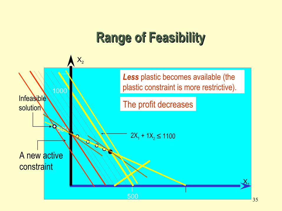
Range of FeasibilityRange of Feasibility
1000
500
X2
X1
5002X1 + 1X2 ≤ 1100
Less plastic becomes available (the plastic constraint is more restrictive).
The profit decreases
A new activeconstraint
Infeasiblesolution
36
– Sunk costs: The shadow price is the value of an extra unit of the resource, since the cost of the resource is not included in the calculation of the objective function coefficient.
– Included costs: The shadow price is the premium value above the existing unit value for the resource, since the cost of the resource is included in the calculation of the objective function coefficient.
The correct interpretation of shadow prices The correct interpretation of shadow prices

37
Other Post - Optimality Changes Other Post - Optimality Changes
• Addition of a constraint.
• Deletion of a constraint.
• Addition of a variable.
• Deletion of a variable.
• Changes in the left - hand side coefficients.
38
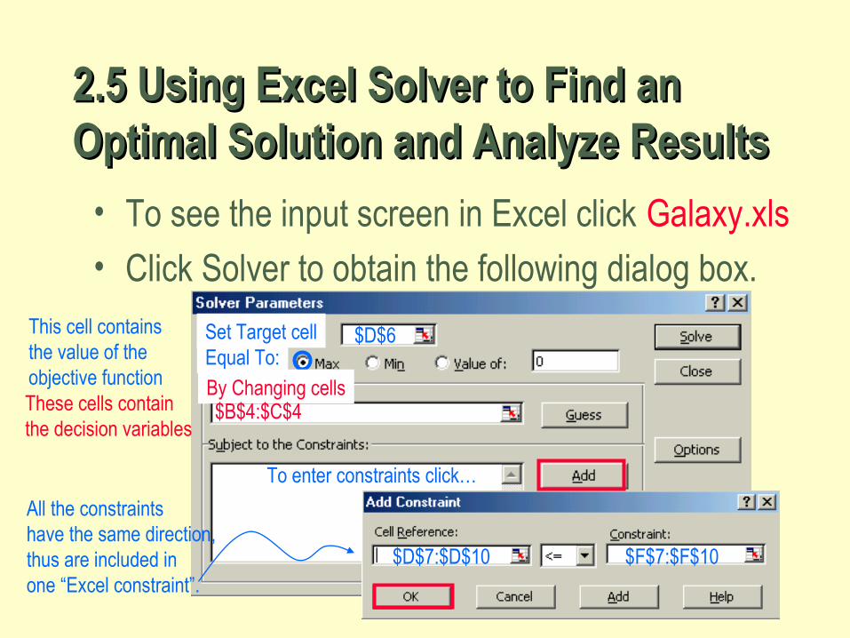
2.5 Using Excel Solver to Find an 2.5 Using Excel Solver to Find an Optimal Solution and Analyze ResultsOptimal Solution and Analyze Results
• To see the input screen in Excel click Galaxy.xls• Click Solver to obtain the following dialog box.
Equal To:
By Changing cellsThese cells containthe decision variables
$B$4:$C$4
To enter constraints click…
Set Target cell $D$6This cell contains the value of the objective function
$D$7:$D$10 $F$7:$F$10
All the constraintshave the same direction, thus are included in one “Excel constraint”.

39
Using Excel SolverUsing Excel Solver
• To see the input screen in Excel click Galaxy.xls• Click Solver to obtain the following dialog box.
Equal To:
$D$7:$D$10<=$F$7:$F$10
By Changing cellsThese cells containthe decision variables
$B$4:$C$4
Set Target cell $D$6This cell contains the value of the objective function
Click on ‘Options’and check ‘Linear Programming’ and‘Non-negative’.

40
• To see the input screen in Excel click Galaxy.xls• Click Solver to obtain the following dialog box.
Equal To:
$D$7:$D$10<=$F$7:$F$10
By Changing cells$B$4:$C$4
Set Target cell $D$6
Using Excel SolverUsing Excel Solver

41
Space Rays ZappersDozens 320 360
Total LimitProfit 8 5 4360
Plastic 2 1 1000 <= 1000Prod. Time 3 4 2400 <= 2400
Total 1 1 680 <= 700Mix 1 -1 -40 <= 350
GALAXY INDUSTRIES
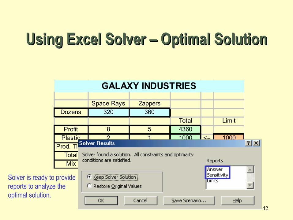
Using Excel Solver – Optimal SolutionUsing Excel Solver – Optimal Solution
42
Space Rays ZappersDozens 320 360
Total LimitProfit 8 5 4360
Plastic 2 1 1000 <= 1000Prod. Time 3 4 2400 <= 2400
Total 1 1 680 <= 700Mix 1 -1 -40 <= 350
GALAXY INDUSTRIES
Using Excel Solver – Optimal SolutionUsing Excel Solver – Optimal Solution
Solver is ready to providereports to analyze theoptimal solution.
43
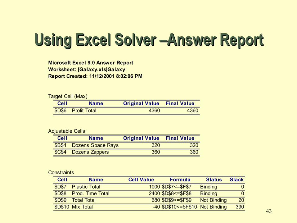
Using Excel Solver –Answer ReportUsing Excel Solver –Answer ReportMicrosoft Excel 9.0 Answer ReportWorksheet: [Galaxy.xls]GalaxyReport Created: 11/12/2001 8:02:06 PM
Target Cell (Max)Cell Name Original Value Final Value
$D$6 Profit Total 4360 4360
Adjustable CellsCell Name Original Value Final Value
$B$4 Dozens Space Rays 320 320$C$4 Dozens Zappers 360 360
Constraints
Cell Name Cell Value Formula Status Slack$D$7 Plastic Total 1000 $D$7<=$F$7 Binding 0$D$8 Prod. Time Total 2400 $D$8<=$F$8 Binding 0$D$9 Total Total 680 $D$9<=$F$9 Not Binding 20$D$10 Mix Total -40 $D$10<=$F$10 Not Binding 390
44
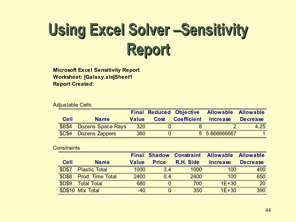
Using Excel Solver –Sensitivity Using Excel Solver –Sensitivity ReportReport
Microsoft Excel Sensitivity ReportWorksheet: [Galaxy.xls]Sheet1Report Created:
Adjustable CellsFinal Reduced Objective Allowable Allowable
Cell Name Value Cost Coefficient Increase Decrease$B$4 Dozens Space Rays 320 0 8 2 4.25$C$4 Dozens Zappers 360 0 5 5.666666667 1
ConstraintsFinal Shadow Constraint Allowable Allowable
Cell Name Value Price R.H. Side Increase Decrease$D$7 Plastic Total 1000 3.4 1000 100 400$D$8 Prod. Time Total 2400 0.4 2400 100 650$D$9 Total Total 680 0 700 1E+30 20$D$10 Mix Total -40 0 350 1E+30 390
45
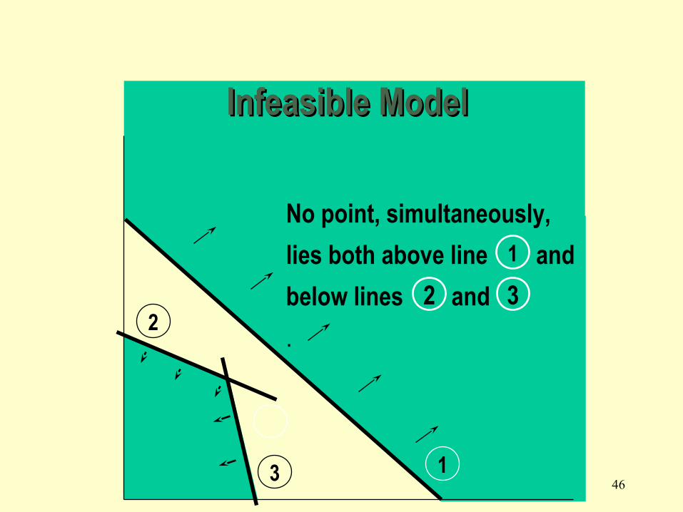
• Infeasibility: Occurs when a model has no feasible point.
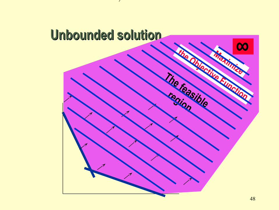
• Unboundness: Occurs when the objective can become
infinitely large (max), or infinitely small (min).
• Alternate solution: Occurs when more than one point
optimizes the objective function
2.7 Models Without Unique Optimal 2.7 Models Without Unique Optimal SolutionsSolutions
46
1
No point, simultaneously,
lies both above line and
below lines and
.
1
2 32
3
Infeasible ModelInfeasible Model

47
Solver – Infeasible ModelSolver – Infeasible Model
48
Unbounded solutionUnbounded solution
The feasible
region
Maximize
the Objective Function
∞
49
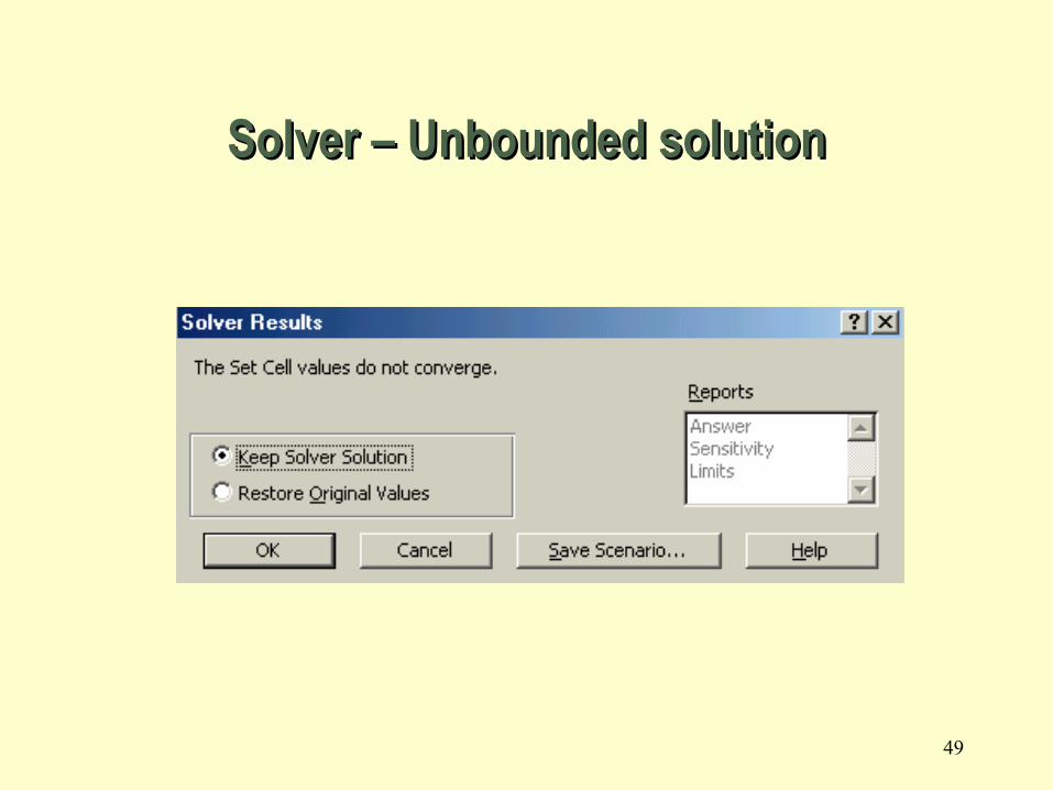
Solver – Unbounded solutionSolver – Unbounded solution
50
• Solver does not alert the user to the existence of alternate optimal solutions.
• Many times alternate optimal solutions exist when the allowable increase or allowable decrease is equal to zero.
• In these cases, we can find alternate optimal solutions using Solver by the following procedure:
Solver – An Alternate Optimal SolutionSolver – An Alternate Optimal Solution
51
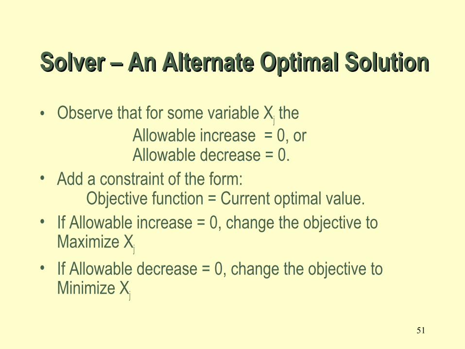
• Observe that for some variable Xj the Allowable increase = 0, orAllowable decrease = 0.
• Add a constraint of the form:Objective function = Current optimal value.
• If Allowable increase = 0, change the objective to Maximize Xj
• If Allowable decrease = 0, change the objective to Minimize Xj
Solver – An Alternate Optimal SolutionSolver – An Alternate Optimal Solution

52
2.8 Cost Minimization Diet Problem 2.8 Cost Minimization Diet Problem
• Mix two sea ration products: Texfoods, Calration.• Minimize the total cost of the mix. • Meet the minimum requirements of Vitamin A, Vitamin D, and Iron.

53
• Decision variables– X1 (X2) -- The number of two-ounce portions of
Texfoods (Calration) product used in a serving.
• The ModelMinimize 0.60X1 + 0.50X2
Subject to
20X1 + 50X2 ≥ 100 Vitamin A
25X1 + 25X2 ≥ 100 Vitamin D
50X1 + 10X2 ≥ 100 Iron
X1, X2 ≥ 0
Cost per 2 oz.
% Vitamin Aprovided per 2 oz.
% required
Cost Minimization Diet Problem Cost Minimization Diet Problem
54
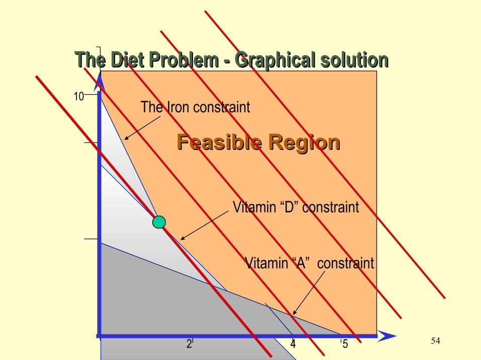
10
2 44 5
Feasible RegionFeasible Region
Vitamin “D” constraint
Vitamin “A” constraint
The Iron constraint
The Diet Problem - Graphical solutionThe Diet Problem - Graphical solution
55
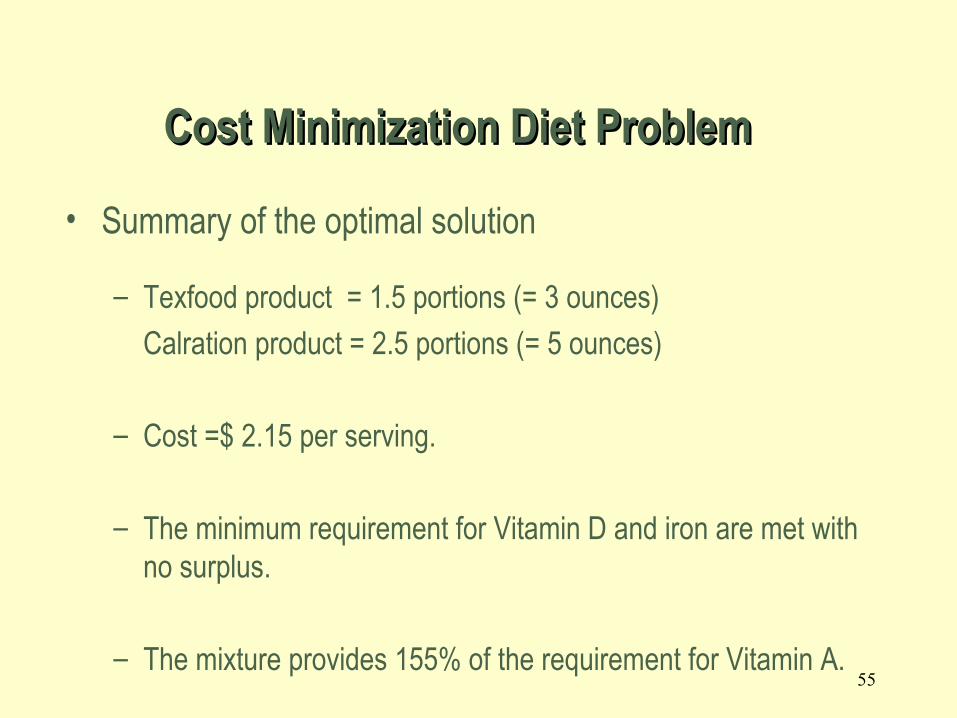
• Summary of the optimal solution
– Texfood product = 1.5 portions (= 3 ounces)
Calration product = 2.5 portions (= 5 ounces)
– Cost =$ 2.15 per serving.
– The minimum requirement for Vitamin D and iron are met with
no surplus.
– The mixture provides 155% of the requirement for Vitamin A.
Cost Minimization Diet Problem Cost Minimization Diet Problem
56
• Linear programming software packages solve large linear models.
• Most of the software packages use the algebraic technique called the Simplex algorithm.
• The input to any package includes:– The objective function criterion (Max or Min).– The type of each constraint: .– The actual coefficients for the problem.
Computer Solution of Linear Programs With Computer Solution of Linear Programs With Any Number of Decision VariablesAny Number of Decision Variables
≤ = ≥, ,
ReferencesReferences
• Quantitative Techniques, by CR Kothari, Vikas publication
• Fundamentals of Statistics by SC Guta Publisher Sultan Chand
• Quantitative Techniques in management by N.D. Vohra Publisher: Tata Mcgraw hill
57


