6.1McGraw-Hill/Irwin
P&T Company Distribution Problem
CANNERY 1 Bellingham
CANNERY 2 Eugene
WAREHOUSE 1 Sacramento
WAREHOUSE 2 Salt Lake City
WAREHOUSE 3 Rapid City
WAREHOUSE 4 Albuquerque
CANNERY 3 Albert Lea
6.2McGraw-Hill/Irwin
Shipping Data
Cannery Output Warehouse Allocation
Bellingham 75 truckloads Sacramento 80 truckloads
Eugene 125 truckloads Salt Lake City 65 truckloads
Albert Lea 100 truckloads Rapid City 70 truckloads
Total 300 truckloads Albuquerque 85 truckloads
Total 300 truckloads
6.3McGraw-Hill/Irwin
Current Shipping Plan
Warehouse
From \ To Sacramento Salt Lake City Rapid City Albuquerque
Cannery
Bellingham 75 0 0 0
Eugene 5 65 55 0
Albert Lea 0 0 15 85
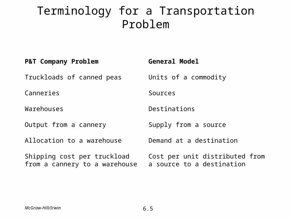
6.4McGraw-Hill/Irwin
Shipping Cost per Truckload
Warehouse
From \ To Sacramento Salt Lake City Rapid City Albuquerque
Cannery
Bellingham $464 $513 $654 $867
Eugene 352 416 690 791
Albert Lea 995 682 388 685
Total shipping cost = 75($464) + 5($352) + 65($416) + 55($690) + 15($388) + 85($685)= $165,595
6.5McGraw-Hill/Irwin
Terminology for a Transportation Problem
P&T Company Problem
Truckloads of canned peas
Canneries
Warehouses
Output from a cannery
Allocation to a warehouse
Shipping cost per truckload from a cannery to a warehouse
General Model
Units of a commodity
Sources
Destinations
Supply from a source
Demand at a destination
Cost per unit distributed from a source to a destination
6.6McGraw-Hill/Irwin
Characteristics of Transportation Problems
• The Requirements Assumption– Each source has a fixed supply of units, where this entire supply must be distributed
to the destinations.
– Each destination has a fixed demand for units, where this entire demand must be received from the sources.
• The Feasible Solutions Property– A transportation problem will have feasible solutions if and only if the sum of its
supplies equals the sum of its demands.
• The Cost Assumption– The cost of distributing units from any particular source to any particular
destination is directly proportional to the number of units distributed.
– This cost is just the unit cost of distribution times the number of units distributed.
6.7McGraw-Hill/Irwin
The Transportation Model
Any problem (whether involving transportation or not) fits the model for a transportation problem if
1. It can be described completely in terms of a table like Table 6.5 that identifies all the sources, destinations, supplies, demands, and unit costs, and
2. satisfies both the requirements assumption and the cost assumption.
The objective is to minimize the total cost of distributing the units.
6.8McGraw-Hill/Irwin
The P&T Co. Transportation Problem
Unit Cost
Destination(Warehouse): Sacramento Salt Lake City Rapid City Albuquerque Supply
Source (Cannery)
Bellingham $464 $513 $654 $867 75
Eugene 352 416 690 791 125
Albert Lea 995 682 388 685 100
Demand 80 65 70 85
6.9McGraw-Hill/Irwin
Spreadsheet Formulation
34567891011121314151617
B C D E F G H I JUnit Cost Destination (Warehouse)
Sacramento Salt Lake City Rapid City AlbuquerqueSource Bellingham $464 $513 $654 $867
(Cannery) Eugene $352 $416 $690 $791Albert Lea $995 $682 $388 $685
Shipment Quantity Destination (Warehouse)(Truckloads) Sacramento Salt Lake City Rapid City Albuquerque Total Shipped Supply
Source Bellingham 0 20 0 55 75 = 75(Cannery) Eugene 80 45 0 0 125 = 125
Albert Lea 0 0 70 30 100 = 100Total Received 80 65 70 85
= = = = Total CostDemand 80 65 70 85 $152,535
6.10McGraw-Hill/Irwin
Network Representation
S1
S2
S3
D4
D2
D1
D3
75
125
100
80
65
70
85
Supplies Demands
SourcesDestinations
(Bellingham)
(Eugene)
(Alber t Lea)
(Sacramento)
(Salt Lake City)
(Rapid City)
(Albuquerque)
464513
654867
352 416690
791
995 682
685
388
6.11McGraw-Hill/Irwin
The Transportation Problem is an LP
Let xij = the number of truckloads to ship from cannery i to warehouse j(i = 1, 2, 3; j = 1, 2, 3, 4)
Minimize Cost = $464x11 + $513x12 + $654x13 + $867x14 + $352x21 + $416x22
+ $690x23 + $791x24 + $995x31 + $682x32 + $388x33 + $685x34
subject toCannery 1: x11 + x12 + x13 + x14 = 75Cannery 2: x21 + x22 + x23 + x24 = 125Cannery 3: x31 + x32 + x33 + x34 = 100Warehouse 1: x11 + x21 + x31 = 80Warehouse 2: x12 + x22 + x32 = 65Warehouse 3: x13 + x23 + x33 = 70Warehouse 4: x14 + x24 + x34 = 85
andxij ≥ 0 (i = 1, 2, 3; j = 1, 2, 3, 4)
6.12McGraw-Hill/Irwin
Integer Solutions Property
As long as all its supplies and demands have integer values, any transportation problem with feasible solutions is guaranteed to have an optimal solution with integer values for all its decision variables. Therefore, it is not necessary to add constraints to the model that restrict these variables to only have integer values.
6.13McGraw-Hill/Irwin
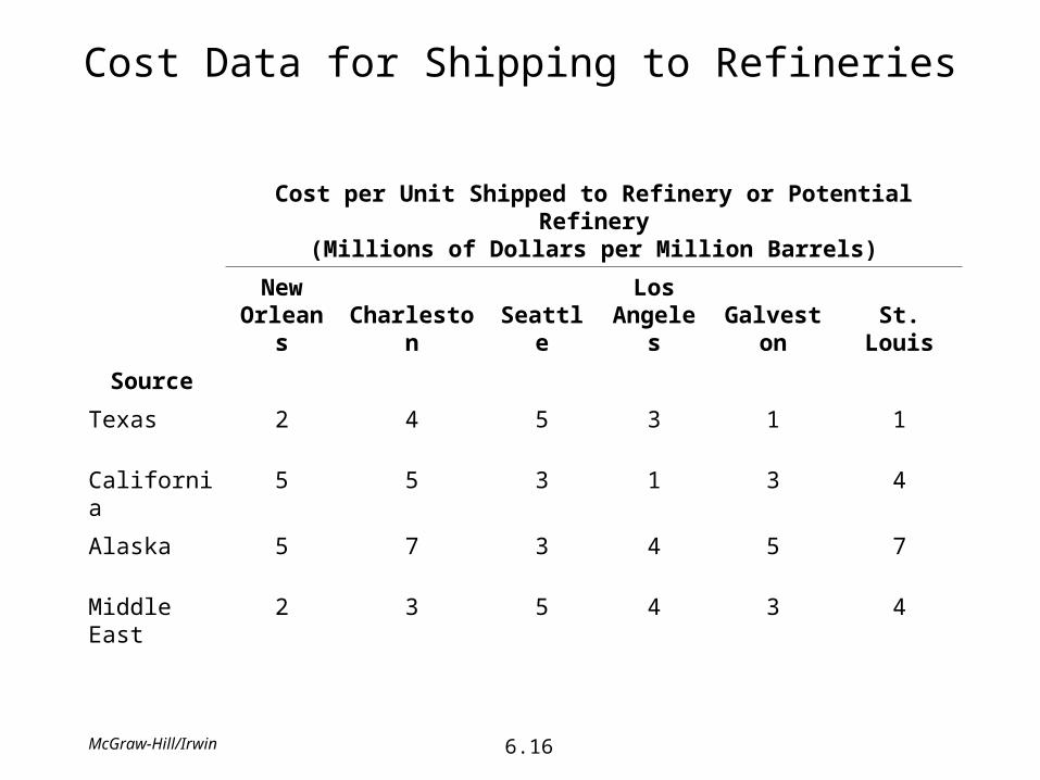
Location of Texago’s Facilities
Type of Facility Locations
Oil fields 1. Several in Texas2. Several in California3. Several in Alaska
Refineries 1. Near New Orleans, Louisiana2. Near Charleston, South Carolina3. Near Seattle, Washington
Distribution Centers 1. Pittsburgh, Pennsylvania2. Atlanta, Georgia3. Kansas City, Missouri4. San Francisco, California
6.14McGraw-Hill/Irwin
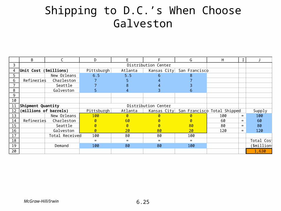
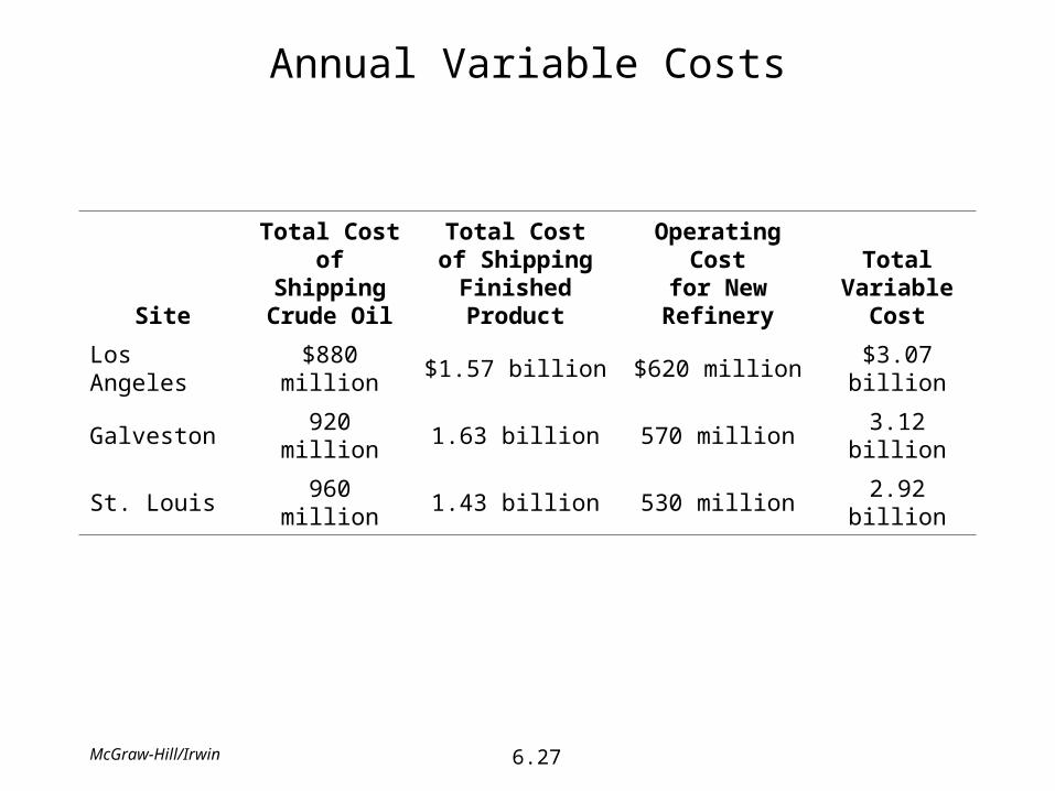
Potential Sites for Texago’s New Refinery
Potential Site Main Advantages
Near Los Angeles, California 1. Near California oil fields.2. Ready access from Alaska oil fields.3. Fairly near San Francisco distribution center.
Near Galveston, Texas 1. Near Texas oil fields.2. Ready access from Middle East imports.3. Near corporate headquarters.
Near St. Louis, Missouri 1. Low operating costs.2. Centrally located for distribution centers.3. Ready access to crude oil via the Mississippi River.
6.15McGraw-Hill/Irwin
Production Data for Texago
Refinery
Crude OilNeeded Annually(Million Barrels) Oil Fields
Crude Oil Produced Annually
(Million Barrels)
New Orleans 100 Texas 80
Charleston 60 California 60
Seattle 80 Alaska 100
New site 120 Total 240
Total 360 Needed imports = 360 – 240 = 120
6.16McGraw-Hill/Irwin
Cost Data for Shipping to Refineries
Cost per Unit Shipped to Refinery or Potential Refinery(Millions of Dollars per Million Barrels)
New Orleans Charleston Seattle
Los Angeles Galveston St. Louis
Source
Texas 2 4 5 3 1 1
California 5 5 3 1 3 4
Alaska 5 7 3 4 5 7
Middle East 2 3 5 4 3 4
6.17McGraw-Hill/Irwin
Cost Data for Shipping to Distribution Centers
Cost per Unit Shipped to Distribution Center(Millions of Dollars)
Pittsburgh Atlanta Kansas City San Francisco
Refinery
New Orleans 6.5 5.5 6 8
Charleston 7 5 4 7
Seattle 7 8 4 3
Potential Refinery
Los Angeles 8 6 3 2
Galveston 5 4 3 6
St. Louis 4 3 1 5
Number of units needed 100 80 80 100
6.18McGraw-Hill/Irwin
Estimated Operating Costs for Refineries
Site Annual Operating Cost(Millions of Dollars)
Los Angeles
Galveston
St. Louis
620
570
530
6.19McGraw-Hill/Irwin
Basic Spreadsheet for Shipping to Refineries
34567891011121314151617181920
B C D E F G H I JRefineries
Unit Cost ($millions) New Orleans Charleston Seattle New SiteTexas 2 4 5
Oil California 5 5 3Fields Alaska 5 7 3
Middle East 2 3 5
Shipment Quantity Refineries(millions of barrels) New Orleans Charleston Seattle New Site Total Shipped Supply
Texas 0 0 0 0 0 = 80Oil California 0 0 0 0 0 = 60
Fields Alaska 0 0 0 0 0 = 100Middle East 0 0 0 0 0 = 120
Total Received 0 0 0 0= = = = Total Cost
Demand 100 60 80 120 ($millions)0
6.20McGraw-Hill/Irwin
Shipping to Refineries, Including Los Angeles
34567891011121314151617181920
B C D E F G H I JRefineries
Unit Cost ($millions) New Orleans Charleston Seattle Los AngelesTexas 2 4 5 3
Oil California 5 5 3 1Fields Alaska 5 7 3 4
Middle East 2 3 5 4
Shipment Quantity Refineries(millions of barrels) New Orleans Charleston Seattle Los Angeles Total Shipped Supply
Texas 40 0 0 40 80 = 80Oil California 0 0 0 60 60 = 60
Fields Alaska 0 0 80 20 100 = 100Middle East 60 60 0 0 120 = 120
Total Received 100 60 80 120= = = = Total Cost
Demand 100 60 80 120 ($millions)880
6.21McGraw-Hill/Irwin
Shipping to Refineries, Including Galveston
34567891011121314151617181920
B C D E F G H I JRefineries
Unit Cost ($millions) New Orleans Charleston Seattle GalvestonTexas 2 4 5 1
Oil California 5 5 3 3Fields Alaska 5 7 3 5
Middle East 2 3 5 3
Shipment Quantity Refineries(millions of barrels) New Orleans Charleston Seattle Galveston Total Shipped Supply
Texas 20 0 0 60 80 = 80Oil California 0 0 0 60 60 = 60
Fields Alaska 20 0 80 0 100 = 100Middle East 60 60 0 0 120 = 120
Total Received 100 60 80 120= = = = Total Cost
Demand 100 60 80 120 ($millions)920
6.22McGraw-Hill/Irwin
Shipping to Refineries, Including St. Louis
34567891011121314151617181920
B C D E F G H I JRefineries
Unit Cost ($millions) New Orleans Charleston Seattle St. LouisTexas 2 4 5 1
Oil California 5 5 3 4Fields Alaska 5 7 3 7
Middle East 2 3 5 4
Shipment Quantity Refineries(millions of barrels) New Orleans Charleston Seattle St. Louis Total Shipped Supply
Texas 0 0 0 80 80 = 80Oil California 0 20 0 40 60 = 60
Fields Alaska 20 0 80 0 100 = 100Middle East 80 40 0 0 120 = 120
Total Received 100 60 80 120= = = = Total Cost
Demand 100 60 80 120 ($millions)960
6.23McGraw-Hill/Irwin
Basic Spreadsheet for Shipping to D.C.’s
34567891011121314151617181920
B C D E F G H I JDistribution Center
Unit Cost ($millions) Pittsburgh Atlanta Kansas City San FranciscoNew Orleans 6.5 5.5 6 8
Refineries Charleston 7 5 4 7Seattle 7 8 4 3
New Site
Shipment Quantity Distribution Center(millions of barrels) Pittsburgh Atlanta Kansas City San Francisco Total Shipped Supply
New Orleans 0 0 0 0 0 = 100Refineries Charleston 0 0 0 0 0 = 60
Seattle 0 0 0 0 0 = 80New Site 0 0 0 0 0 = 120
Total Received 0 0 0 0= = = = Total Cost
Demand 100 80 80 100 ($millions)0
6.24McGraw-Hill/Irwin
Shipping to D.C.’s When Choose Los Angeles
34567891011121314151617181920
B C D E F G H I JDistribution Center
Unit Cost ($millions) Pittsburgh Atlanta Kansas City San FranciscoNew Orleans 6.5 5.5 6 8
Refineries Charleston 7 5 4 7Seattle 7 8 4 3
Los Angeles 8 6 3 2
Shipment Quantity Distribution Center(millions of barrels) Pittsburgh Atlanta Kansas City San Francisco Total Shipped Supply
New Orleans 80 20 0 0 100 = 100Refineries Charleston 0 60 0 0 60 = 60
Seattle 20 0 0 60 80 = 80Los Angeles 0 0 80 40 120 = 120
Total Received 100 80 80 100= = = = Total Cost
Demand 100 80 80 100 ($millions)1,570
6.25McGraw-Hill/Irwin
Shipping to D.C.’s When Choose Galveston
34567891011121314151617181920
B C D E F G H I JDistribution Center
Unit Cost ($millions) Pittsburgh Atlanta Kansas City San FranciscoNew Orleans 6.5 5.5 6 8
Refineries Charleston 7 5 4 7Seattle 7 8 4 3
Galveston 5 4 3 6
Shipment Quantity Distribution Center(millions of barrels) Pittsburgh Atlanta Kansas City San Francisco Total Shipped Supply
New Orleans 100 0 0 0 100 = 100Refineries Charleston 0 60 0 0 60 = 60
Seattle 0 0 0 80 80 = 80Galveston 0 20 80 20 120 = 120
Total Received 100 80 80 100= = = = Total Cost
Demand 100 80 80 100 ($millions)1,630
6.26McGraw-Hill/Irwin
Shipping to D.C.’s When Choose St. Louis
34567891011121314151617181920
B C D E F G H I JDistribution Center
Unit Cost ($millions) Pittsburgh Atlanta Kansas City San FranciscoNew Orleans 6.5 5.5 6 8
Refineries Charleston 7 5 4 7Seattle 7 8 4 3
St. Louis 4 3 1 5
Shipment Quantity Distribution Center(millions of barrels) Pittsburgh Atlanta Kansas City San Francisco Total Shipped Supply
New Orleans 100 0 0 0 100 = 100Refineries Charleston 0 60 0 0 60 = 60
Seattle 0 0 0 80 80 = 80St. Louis 0 20 80 20 120 = 120
Total Received 100 80 80 100= = = = Total Cost
Demand 100 80 80 100 ($millions)1,430
6.27McGraw-Hill/Irwin
Annual Variable Costs
Site
Total Costof ShippingCrude Oil
Total Costof Shipping
Finished Product
Operating Costfor NewRefinery
TotalVariable
Cost
Los Angeles $880 million $1.57 billion $620 million $3.07 billion
Galveston 920 million 1.63 billion 570 million 3.12 billion
St. Louis 960 million 1.43 billion 530 million 2.92 billion