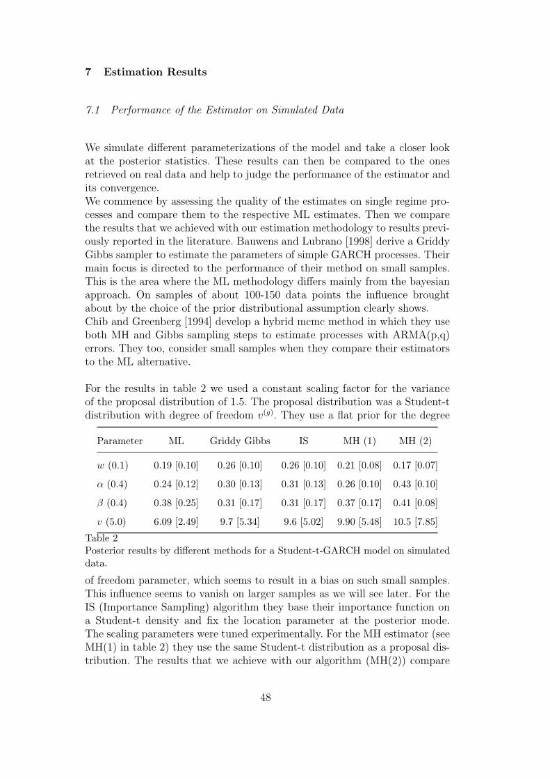
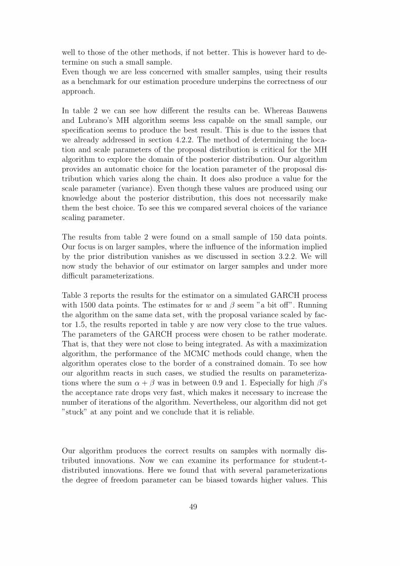
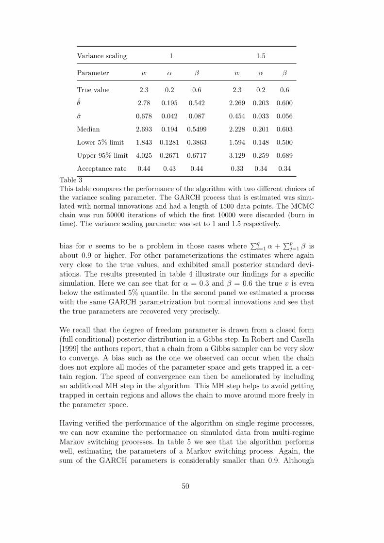
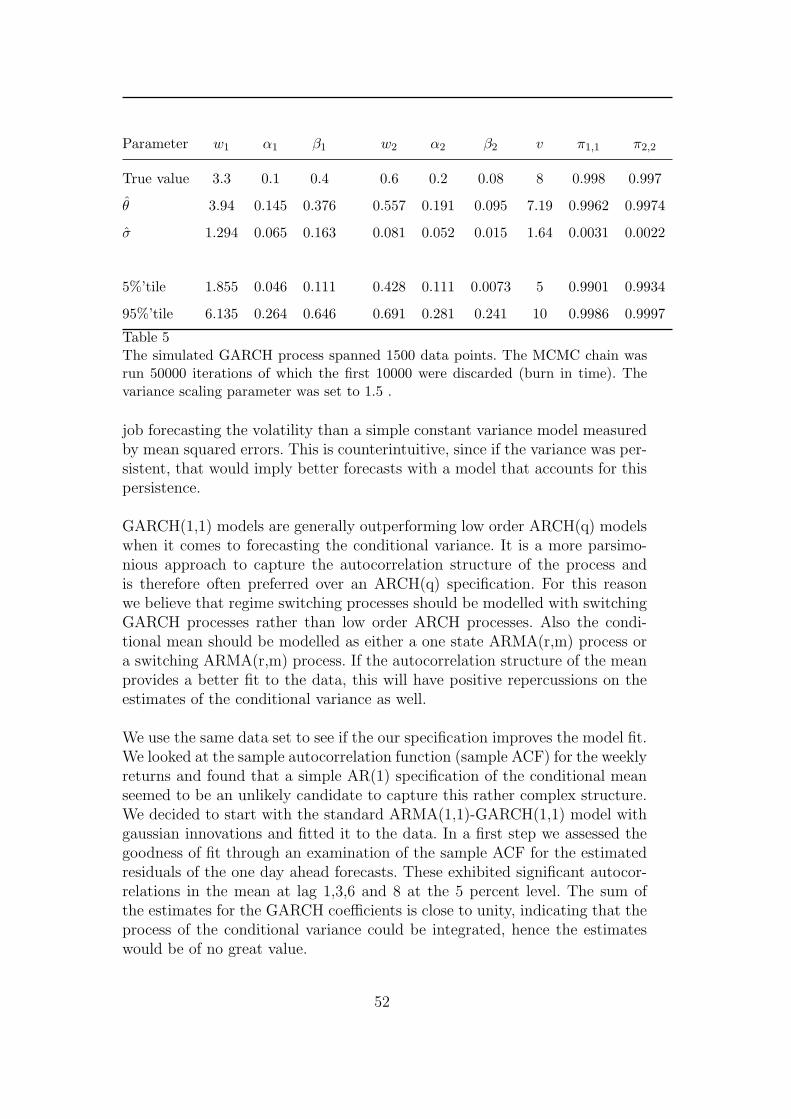
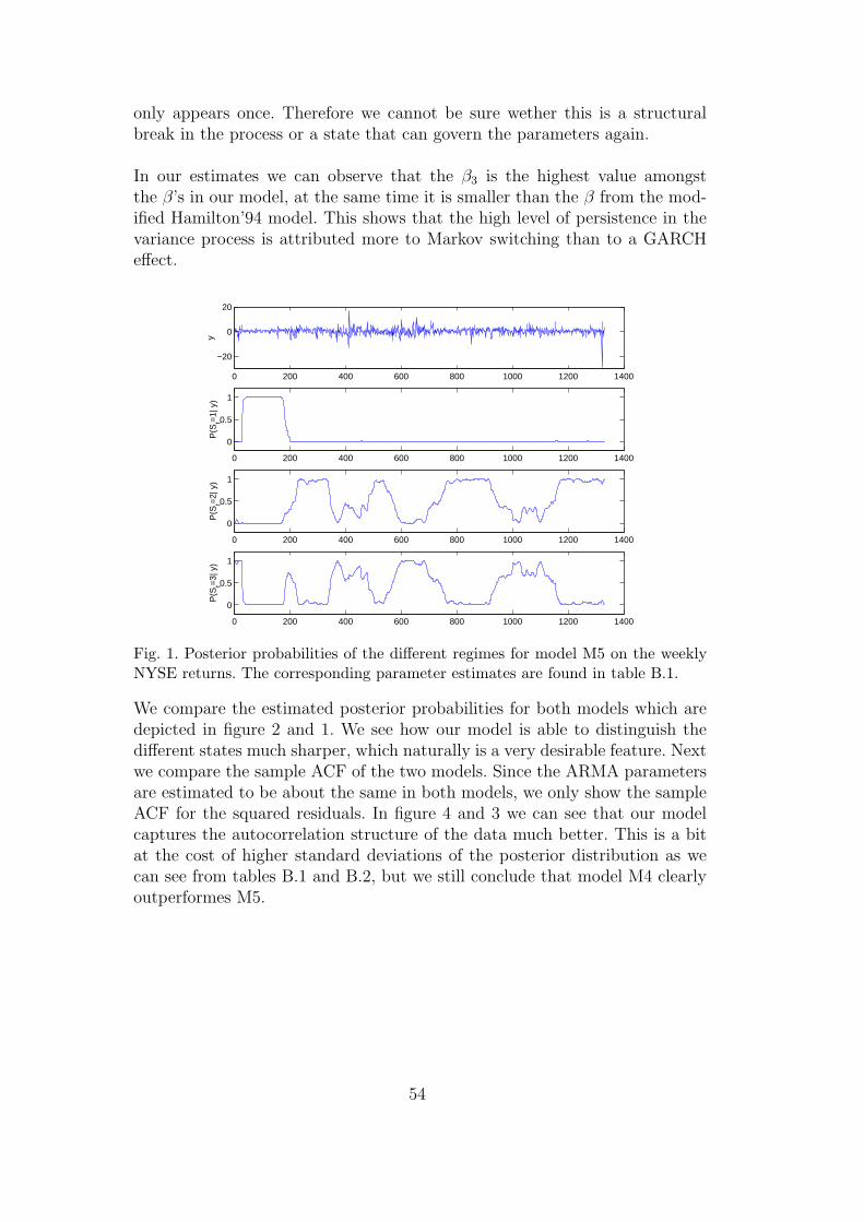
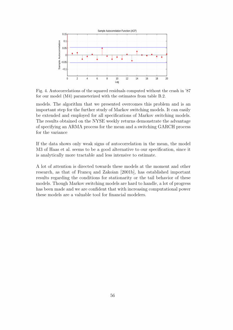
MCMC methods for the estimation of MS-ARMA-GARCH Models Jan S. Henneke a,* , Svetlozar T. Rachev b,1 Frank J. Fabozzi c a University of Karlsruhe WestLB AG London b University of Karlsruhe, Germany University of California, Santa Barbera, USA c Yale School of Management, USA Abstract Regime Switching models, especially Markov switching models, are regarded as a promising way to capture nonlinearities in time series. They can account for sudden changes in the structure of the mean or the variance of a process and give a straightforward interpretation of these shifts. Such shifts would cause regu- lar ARMA-GARCH models to imply non-stationary processes. Combining the ele- ments of Markov switching models with full ARMA-GARCH models poses severe difficulties when it comes to understanding their dynamic properties and for the computation of parameter estimators. Maximum Likelihood estimation can become completely unfeasible due to the full path dependence of such models. Estimation methods such as the EM algorithm can be used for the ML estimation of sim- ple Markov switching AR-ARCH models but become unfeasible if MA or GARCH components are introduced. In this article we formulate a full Markov switching ARMA-GARCH model and estimate based on the Bayesian framework. This facil- itates the use of Markov Chain Monte Carlo methods and allows us to develop an algorithm to compute the Bayes estimator of the regimes and parameters of our model. The approach is illustrated on simulated data and with returns from the New York Stock exchange. Our model is then compared to MS-AR-ARCH variants and proves clearly to be advantageous. Key words: Regime Switching, Markov Switching, Markov Chain Monte Carlo Methods, MCMC, Bayesian Estimation JEL Classification : C11, C13, C51, C52, C63 * Corresponding author. 1 Prof. S.T. Rachev gratefully acknowledges research support by grants from the Division of Mathematical, Life and Physical Sciences, College of Letters and Science, 27 November 2007
Transcript
MCMC methods for the estimation of
MS-ARMA-GARCH Models
Jan S. Henneke a,∗, Svetlozar T. Rachev b,1 Frank J. Fabozzi c
aUniversity of KarlsruheWestLB AG London
bUniversity of Karlsruhe, GermanyUniversity of California, Santa Barbera, USA
cYale School of Management, USA
Abstract
Regime Switching models, especially Markov switching models, are regarded asa promising way to capture nonlinearities in time series. They can account forsudden changes in the structure of the mean or the variance of a process andgive a straightforward interpretation of these shifts. Such shifts would cause regu-lar ARMA-GARCH models to imply non-stationary processes. Combining the ele-ments of Markov switching models with full ARMA-GARCH models poses severedifficulties when it comes to understanding their dynamic properties and for thecomputation of parameter estimators. Maximum Likelihood estimation can becomecompletely unfeasible due to the full path dependence of such models. Estimationmethods such as the EM algorithm can be used for the ML estimation of sim-ple Markov switching AR-ARCH models but become unfeasible if MA or GARCHcomponents are introduced. In this article we formulate a full Markov switchingARMA-GARCH model and estimate based on the Bayesian framework. This facil-itates the use of Markov Chain Monte Carlo methods and allows us to develop analgorithm to compute the Bayes estimator of the regimes and parameters of ourmodel. The approach is illustrated on simulated data and with returns from theNew York Stock exchange. Our model is then compared to MS-AR-ARCH variantsand proves clearly to be advantageous.
∗ Corresponding author.1 Prof. S.T. Rachev gratefully acknowledges research support by grants from theDivision of Mathematical, Life and Physical Sciences, College of Letters and Science,
27 November 2007
1 Introduction
A central property of economic time series, common to many financial timeseries, is that their volatility varies over time. Describing the volatility of anasset is a key issue for researchers in financial economics and analysts in finan-cial markets. The prices of assets depend on the expected volatility (covariancestructure) of the returns and some derivatives depend solely on the correlationstructure of their underlyings. Second, statistical inference about the param-eters of the conditional mean is dependent on the correct specification andestimation of the variance (and vice versa). Banks and other financial insti-tutions apply value-at-risk models to assess risks in their marketable assets.Here a precise specification of a model is needed so that risks are neither overnor underestimated.
The most popular class of models for time varying volatility is representedby GARCH type models. Bollerslev et al. [1992] survey several hundred stud-ies of financial markets with applications of various extensions of the GARCHmodels. The popularity of the GARCH models stem from their ability to par-simoniously capture complex patterns of dependency in the data.
In practical application the estimated GARCH models usually imply a veryhigh level of persistence in the volatility. This lead to the IGARCH model ofBollerslev where the process for the volatility incorporates a unit root. Butwhat if the data actually stems from stationary processes that differ in theirparameters? This question stirred research about structural breaks in stochas-tic processes. It turned out that such changes in the parameters could accountfor a part of the high persistency and disentangle the persistency that stemsfrom changes in the parameters and the one implied by the estimated GARCHmodel. Thus estimates on data from different stationary processes lead to anindication of nonstationarity which lead to methods that describe and test forstructural breaks.
Maekawa et al. [2005] demonstrate that most of the Tokyo stock return datasets posses volatility persistence and in many cases it is a consequence of struc-tural breaks in the GARCH process. Rapach and Strauss [2005] report signif-icant evidence for structural breaks in the unconditional variance of exchangerate returns. Smith finds strong evidence of structural breaks in GARCH mod-els of US index returns, foreign exchange rates, and individual stock returns.He concludes that standard diagnostic tests are no substitute for structuralbreak tests and that the results suggest that more attention needs to be givento structural breaks when building and estimating GARCH models.
University of California, Santa Barbera, the German Research Foundation (DFG)and the German Academic Exchange Service (DAAD).
2
Another approach to this problem would be to describe changes in the pa-rameters endogenously with a Markov Switching model. These models wereintroduced to the econometric mainstream by the seminal article of Hamilton[1989].The difference is that the process can leave a state (parameter set) and returnswith a positive probability. Let us assume, that a process has a ”normal” stateand several other states with higher or lower volatilities. A structural breakmodel will base its parameter estimates only on the data between changesin the structure and throws away the rest of the data. In such a scenario aMarkov Switching model would retrieve much better estimates for the ”nor-mal” state, because it operates on a much larger data set. In this case theMarkov Switching model would yield a superior fit and more important, abetter forecasting performance.
Markov Switching models are currently being considered for various markets.One example are the electricity markets, where the prices exhibit extremejumps. These are due to generator outages, network problems or sudden in-creases in the demand. All of these represent exogenous events, which wouldrepresent the current regime of the price process, and suggest the use of MarkovSwitching models.FX markets are subject to changes in the monetary policies of different coun-tries. Changes in these policies that are triggered by external events can causea change in the level of the variance, thus these economic series are also acandidate for the modelling with Markov Switching models.
In financial markets, spread products are becoming increasingly popular, suchas a derivative paying X times the amount of the spread between the tenand two year swaprate: X × (s(t, t + 10y) − s(t, t + 2y)). The prices of thesederivatives are extremely sensitive to changes of the correlation between thetwo underlyings.Under certain market conditions, that are again triggered by external events,seemingly uncorrelated processes suddenly become more correlated. This hasstrong implications for the pricing and hedging of derivatives on spreads. Herea Markov Switching framework for the level of the correlation will provide themeans to capture these phenomena and conduct inferences about the currentlevel.
While these effects are related to pricing and hedging in the derivatives mar-kets, one naturally finds applications in the risk management of a portfolio.Modern portfolio theory is build on the concept of diversification, therefore acompelling reason for investing in certain funds, is the fact that their returnsseem relatively uncorrelated with market indexes such as the S&P 500. InChan et al. [2005] the authors describe how this diversification argument hadto be reviewed for hedge funds by the lessons of the summer of 1998 when the
3
default in Russian government debt triggered a global flight to quality. Thischanged many of the correlations overnight from 0 to 1.
For the successful application of Markov-Switching models to these problems,it is crucial to have reliable parameter estimators. In econometrics the usualroute to derive parameter estimates is to choose the maximum likelihood ap-proach. However it turned out that this approach becomes computationallyinfeasible for Markov-Switching ARMA-GARCH models and researchers suchas Cai and Hamilton have dismissed these models as too untractable. Insteadthey use low order MS-AR-ARCH models for which they derived estimators. Aconsiderable amount of research in the econometric society is currently beingdevoted to Markov-Switching models as these are perceived to be very promis-ing by an ever growing amount of researchers and practitioners. On difficultdata sets the simpler low order MS-AR-ARCH models do not yield the desiredresults and the need for advanced diagnostics and more sophisticated modelsrises.
In this paper we develop an algorithm for the estimation of the parametersof a full MS-ARMA-GARCH model. For this we chose the bayesian frame-work to formulate the estimator since this enables the application of MarkovChain Monte Carlo methods which are very powerful tools for the numericalcomputation of integrals. We proceed as follows: in section 2 we present sev-eral Markov Switching models and highlight their characteristics. In section3 we briefly review the theory of bayesian estimation to prepare the groundfor an introduction to Markov Chain Monte Carlo Methods in section 4. Withthose methods at hand we derive our estimation algorithm for the MS-ARMA-GARCH model in section 5. Thereafter we briefly present a diagnostic toolfor the convergence of Markov Chain Monte Carlo method in section 6, beforewe evaluate our algorithm in section 7 on both simulated and empirical data.Section 8 concludes.
4
2 Markov Switching Models
All of the models exhibited in this section vary only slightly in their formula-tion, but as we will see in later sections, this will have a great impact on theiranalytical tractability and the derivation of estimators for their parameters.All of them specify a number of latent regimes or states, which control the pa-rameters of the process. These states are themselves random and are assumedto follow a discrete S dimensional markov chain Stt∈N which is defined onthe discrete state space 1, 2, . . . ,S with the transition probability matrix
Π =
π1,1 π1,2 . . . π1,S
π2,1. . .
...
πS,1 . . . . . . πS,S
(1)
where πi,j is the probability that the Markov chain goes from state i to j.This is common for all of the models considered in this article.
We will begin with the model proposed in Hamilton [1989]
Model M1 (Hamilton ’89) The state of the economy St follows a two stateMarkov chain with a transition matrix Π as defined in (1). The time seriesyt is modelled as a fourth-order autoregression around one of two constants,µ1 or µ2.
(yt − µSt) =4∑
i=1
φi(yt−i − µSt−i) + εt εt ∼ N(0, σ2)
Hamilton fits this to the the US GDP data and identifies recessions and re-coveries of the business cycle.A popular class of time series models for macroeconomic data such as the GDPis represented by ARMA processes. Macroeconomic data is usually modelledwith an ARMA process, whereas time series of financial returns in the globalmarkets exhibit strong signs of heteroskedasticity. By far the most popularway to model these returns is through a GARCH process. In order to trans-fer the idea of regime switching to financial markets, Hamilton extended hismodel to incorporate ARCH effects.In Hamilton and Susmel [1994] the authors propose the following model toexplain the weekly returns from the New York Stock Excange:
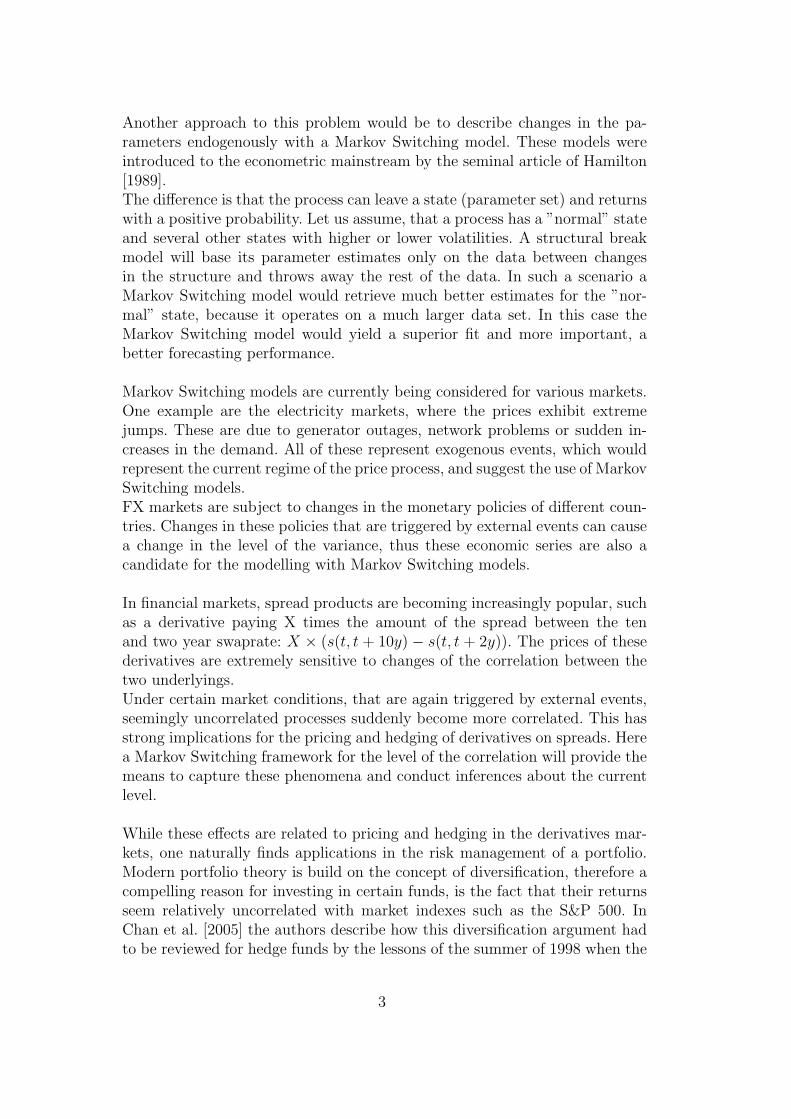
Model M2 (Hamilton ’94) The latent state governing the evolution of themodel parameters is assumed to follow an S dimensional markov chain whose
5
transition matrix is given through (1).
yt = µSt +r∑
i=1
φiyt−i + εt
εt =√
gSt · ut
ut =√
ht · ut ut ∼ t(v)
ht = a0 +q∑
i=1
aiu2t−i + dt−1l1 · u2
t−1
dt−1 =1[ut−1 ≤ 0]
where the φi are the regression coefficients and ai, gi, l1 are positive scalars.
gSt is a state dependent amplifier of the conditional variance. Since ht is definedon the pre-amplified residuals, the conditional variance of ut is thus modelledas a standard ARCH(q) process with a leverage effect. The idea is thus tomodel changes in regime of the conditional variance process as changes in thescale of the process. The dependency structure within each regime will remainunchanged since all values are amplified equally.The specification of the leverage effect through the dummy regression variabledt−1 is taken form Glosten et al. [1989]. This effect is often observed in finan-cial data, where markets react more volatile to negative shocks.The conditional mean is modelled as an AR(r) process with regime switchingmeans µSt .Low order GARCH specifications of the conditional variance offer a much moreparsimonious representation than higher order ARCH models while they areable to capture an equally complex autocorrelation structure. That is the rea-son why they are usually preferred by practitioners. It therefore seems like astep back, to have only the ARCH component in a Markov switching model.But the GARCH component poses significant drawbacks in the estimationprocess when the maximum likelihood route is chosen. Hamilton dismissedMS-GARCH models as untractable and computationally to intensive, there-fore he chose to model the conditional variance with higher order ARCH pro-cesses.
Through a different specification Gray [1996] is able to compute ML esti-mates of a Model which allows for ARMA and GARCH effects. But we canonly speak of effects, since the model differs considerably from a classicalARMA-GARCH model, and properties such as stationarity cannot be trans-ferred directly to the new specification. Furthermore he suggests to asses thegoodness of fit through the Ljung-Box Q Test, applied to the estimated resid-uals. However, the residuals estimated trough his method are not i.i.d. andtherefore the LBQ Test is likely to be spurious. Haas et al. [2004] also criticize
6
this model specification since the conditional variance does not only dependon the past i.i.d. innovations but also on shocks caused by a change in regime.
In Haas et al. [2004] the authors propose a different formulation of the condi-tional variance process. This specifications allows the authors to derive ana-lytical stationarity conditions and straightforward parameter estimators.
Model M3 (Haas ’04) Let the univariate time series εt be given by
εt =√
ht(St) · ut ut ∼ N(0, 1)
where the conditional variance ht is an S ×1 dimensional vector process givenby
ht = α0 + α1ε2t−1 + βht−1
with
αi =
αi,1
αi,2
...
αi,S
β = diag(β1, β2, . . . , βS)
where ht(St) denotes the element of ht at position St.
The conditional variances of the regimes run in parallel and affect each otheronly through the realized values of the innovations. In contrast to model M2it does not impose the same dependency structure for all regimes. It ratherallows a clear-cut interpretation of the variance dynamics in each regime. Theauthors argue that it is the primary feature of a GARCH model, that shocksdrive the volatility and that it can parsimoniously represent high-order ARCHmodels. A shift in the regime will therefore affect the conditional variance pro-cess only through the realized shock εt, whose variance is different. Thereforethey speak of this as the ”natural” generalization of the ARCH approach to aregime switching setting. Furthermore they also present closed form volatilityforecasts.The drawback of this model is, that it is only analytically tractable, as long asno process is specified for the conditional mean. For exchange rate dynamics,this is an appealing model, since the logarithmic percentage returns of themajor exchange rates show no significant autocorrelations in the mean. Thisis different for returns on stocks or interest rates.
In Francq and Zakoian [2001b],Francq and Zakoian [2001a] and Francq and Za-koian [2002] the autors discuss the stationarity properties of markov switchingprocesses, existence of moments and give estimators of the parameters basedon the GMM technique. However, moment estimators do not give smoothed
7
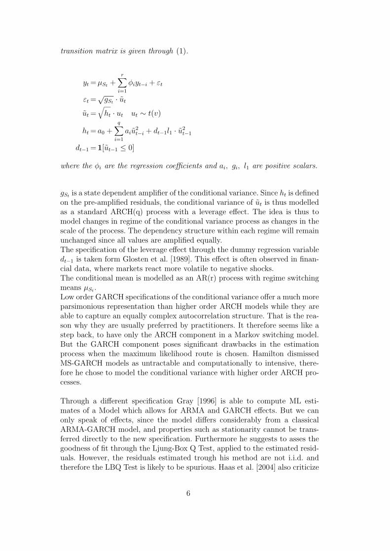
estimates of the states from the latent process. But it is one major aim of theMarkov switching model, to provide both a model that captures characteristicsof a time series and a ”story”. Their specification of a MS-ARMA-GARCHmodel is the same as that of M4, which is the straightforward extension ofHamiltons original regime switching model. This is the model specification forwhich we will derive our Bayesian MCMC estimator in the later sections.
Model M4 We assume that the state of the economy, St follows a discreteS dimensional markov chain with transition probability matrix given by (1).We will now consider an ARMA-GARCH model who’s parameters are depen-dent on the state of this markov chain.
yt = cSt +r∑
i=1
φi(St) · yt−i + εt +m∑
j=1
ψj(St) · εt−j (2a)
ht = ωSt +q∑
i=1
αi(St) · ε2t−i +
p∑
j=1
βj(St) · ht−j (2b)
εt =√
ht · ut ut ∼ N(0, 1)
We will then succeedingly extend the model. In a first step we will let theinnovations εt follow a student-t distribution and in a second step we includea leverage effect in the GARCH component. In the full model the conditionalvariance then becomes
ht = ωSt +q∑
i=1
αi(St) · ε2t−i +
q∑
k=1
dk · lk(St)ε2t−k +
p∑
j=1
βj(St) · ht−j
where dk is 1[εt−k ≤ 0].
As we can see, there are many ways in which one can formulate a Markov-Switching Model, even within these categories one can choose between differ-ent specifications. We talk about different specifications when we distinguishtwo models from the same category, but with a different number of parame-ters. An ARMA(1,1) and an ARMA(2,1) are two different specifications of anARMA(r,m) model.
8
3 Bayesian Estimation
Since bayesian estimation is not the mainstream inference technique, we givea short introduction to this topic.
In the parametric frequentist paradigm data stems from a statistical modelwith fixed parameters. These parameters are totally inaccessible. The bayesianparadigm is fundamentally different in this respect. The parameters of themodel are also assumed to follow a distributional assumption, which is as-sumed by the statistician. This distribution which is referred to as the priordistribution summarizes the prior beliefs of the researcher. The only thingthat is considered real is the observed data. The data itself is also assumedto follow a statistical law. The assumption about the type of distribution isalso an expression of a belief. Inference about the distribution that generatedthe data is therefore the transition of a prior belief into a posterior belief.The bayes theorem formalizes this process of updating a prior belief throughthe observed data set into a posterior belief. Robert [1994] formulates thebayesian paradigm as a duality principle: compared with probabilistic model-ing, the purpose of a statistical analysis is fundamentally an inversion purpose,since it aims at retrieving the causes (parameters of the probabilistic generat-ing mechanism) from the effects (observations). A general description of theinversion of probabilities is given by Bayes theorem: if A and E are eventssuch that P (E) 6= 0, P (A|E) and P (E|A) are related by
P (A|E) =P (E|A)P (A)
P (E|A)P (A) + P (E|Ac)P (Ac)
Bayes and Laplace considered that the uncertainty on the parameters θ couldbe modeled through a probability distribution p(θ) on the parameter spaceΘ. The inversion is then described through an application of Bayes theoremto the full model, as a posterior distribution is computed conditional on theobserved data x
p(θ|x) =f(x|θ)p(θ)∫f(x|θ)p(θ)dθ
(3)
where f is the likelihood of the assumed probabilistic model that generatesthe data. Since the integral in the denominator is only a constant and thenominator is enough to determine the distributional family of the posterior, itis common in the bayesian literature to use the notion of proportionality andwrite (3) as
p(θ|x) ∝ p(θ)f(x|θ).A bayesian statistical model is therefore defined as follows ( Robert [1994]):
Definition 3.1 A Bayesian statistical model is made of a parametric statis-tical model, f(x|θ), and a prior distribution on the parameters, p(θ).
9
The parameters of the prior distribution are usually called hyperparameters.The bayesian paradigm in statistical modelling is based on the same measuretheoretic results as frequentist models, but it differs conceptually in the issueof inference.
3.1 Conjugate Priors
When a statistical model is to be employed, one has to make a choice aboutthe data generating distribution. In a bayesian setting one also has to choosea prior distribution. This prior distribution should hold the prior informationabout the parameters. For a given parameter it mainly reflects the beliefswhere the parameter is expected and how sure one is about that. The roughposition of the parameter is expressed through the mean, whereas the varianceexpresses the prior uncertainty. These are only the beliefs about the two firstmoments of a possible prior distribution, but one has to choose an entire dis-tribution. For this choice of the class or family of the prior, several approacheshave emerged in the bayesian literature. Seemingly the most prominent ofthese is the principle of conjugate priors.
Let f be a likelihood function f(θ|x). A class C of prior distributions is saidto form a conjugate family if the posterior density
p(θ|x) ∝ p(θ)f(θ|x)
is in the class C for all x whenever the prior density is in C.
To give an example we give the conjugate priors for the mean and the varianceof a normal distribution: if
x ∼ N(θ, σ2) θ ∼ N(θ0, σ20)
then the likelihoods are
p(θ) =1√
2πσ0
exp
−(θ − θ0)
2
σ20
(4)
f(x|θ) =1√2πσ
exp
−(x− θ)2
σ2
(5)
hence
p(θ|x) ∝ exp
−θ2
2
(1
σ20
+1
σ2
)+ θ
(θ0
σ20
+x
σ2
)
with
σ21 =
1
σ−20 + σ−2
θ1 = σ21
(θ0
σ20
+x
σ2
)(6)
10
we can write
p(θ|x) ∝ exp
−(θ − θ1)
2
2σ21
and since a density must integrate to one, it follows that
θ|x ∼ N(θ1, σ21) (7)
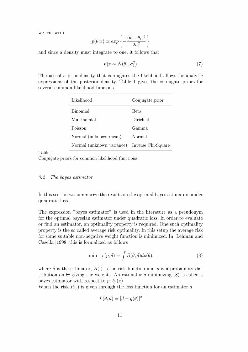
The use of a prior density that conjugates the likelihood allows for analyticexpressions of the posterior density. Table 1 gives the conjugate priors forseveral common likelihood funcions.
Likelihood Conjugate prior
Binomial Beta
Multinomial Dirichlet
Poisson Gamma
Normal (unknown mean) Normal
Normal (unknown variance) Inverse Chi-Square
Table 1Conjugate priors for common likelihood functions
3.2 The bayes estimator
In this section we summarize the results on the optimal bayes estimators underquadratic loss.
The expression ”bayes estimator” is used in the literature as a pseudonymfor the optimal bayesian estimator under quadratic loss. In order to evaluateor find an estimator, an optimality property is required. One such optimalityproperty is the so called average risk optimality. In this setup the average riskfor some suitable non-negative weight function is minimized. In Lehman andCasella [1998] this is formalized as follows
min r(p, δ) =∫
R(θ, δ)dp(θ) (8)
where δ is the estimator, R(.) is the risk function and p is a probability dis-tribution on Θ giving the weights. An estimator δ minimizing (8) is called abayes estimator with respect to p: δp(x)When the risk R(.) is given through the loss function for an estimator d
L(θ, d) = [d− g(θ)]2
11
then the optimal estimator with respect to p is
δp(x) = E[g(Θ)|x]
where g(θ) is usually taken to be θ. The optimal bayes estimator underquadratic loss is therefore simply the posterior mean.
3.2.1 Analytical Bayes Estimators for selected Models
In 3.1 we computed the posterior distribution of a bayesian model of a normalrandom variable with a conjugate prior. The posterior distribution was againnormal and the posterior moments are given through (6). So that for a normalrandom variable with known variance, the bayes estimator for the mean is θ1
from (6). For a sample x = (x1, x2, . . . , xn), where Xi ∼ N(θ, σ2) with knownvariance and unknown mean, the posterior moments are found analogue to(6)
σ21 = (
1
σ20
+n
σ2)−1 (9)
θ1 = σ21
(θ0
σ20
+n · xσ2
)(10)
Normal variance
Let x = (x1, x2, . . . , xn) be a sample from a normal distribution with knownmean µ but unknown variance. Then the likelihood is
f(x|σ2) =n∏
i=1
1√2πσ
exp
−(xi − µ)2
2σ2
∝σ−nexp
−
n∑
i=1
(xi − µ)2
2σ2
We write
S =n∑
i=1
(xi − µ)2
so the posterior is
p(σ2|x) ∝ σ2·(−n/2)exp− S
2σ2
A conjugate prior is then given by
p(σ2) ∝ σ2·(−k/2)exp− S0
2σ2
12
If we substitute k = v + 2 we can write this as
p(σ2|x) ∝ (σ2)−(v+n)/2−1exp−S + S0
2σ2
which is proportional to an inverse chi-squared distribution (χ−2). For theposterior distribution of σ2 one finds
σ2 ∼ (S0 + S)χ−2v+n (11)
which is a scaled inverse chi-square distribution [see also Lee, 2003]. We willneed these results again in section B.1.
3.2.2 Asymptotics of the bayes estimator
This section states the main asymptotic results of bayesian estimation underquadratic loss. We will see that for large n, the estimator converges to the MLestimator.
In a bayesian model one imposes a distribution on the parameter space. Thisseems to contrast drastically with the frequentist approach, where the worldof the parameters is completely determined a priori. However, the data is alsoassumed to be generated by a distribution whose parameters are fixed just asin the frequentist setting. The difference is only that the parameters in the fre-quentist world are inaccessible, whereas in the bayesian setting, a belief aboutthe parameters is expressed through a prior distribution. But at the bottomline both paradigms try to estimate the true data generating parameters θ0.
ML estimators are asymptotically efficient and normally distributed. The sameholds for the bayesian estimator under quadratic loss, independent of the priordistribution. The following theorem and its proof can be found in [Lehmanand Casella, 1998, Theorem 8.3]:
Theorem 3.1 If the regularity conditions (A1)-(A5) hold, and if θn is theBayes estimator when the prior density is p and the loss is squared error, then
√n(θn − θ0)
D−→ N(0, 1/I(θ0)),
so that θn is consistent and asymptotically efficient.
13
3.3 Bayesian Estimation of a Markov Switching Model
In order to compute the bayes estimator for the parameters of model M4, weneed to specify the full bayesian statistical model. The model specificationand the distributional assumption of the innovations yield an expression forthe likelihood conditional on the observed data. It remains to specify the priordistributions for the individual parameters. Here we will choose conjugate pri-ors wherever possible and normal priors with adequate hyperparameters inthe other cases. Since we will work on large data sets, we do not consider thechoice of the prior distribution as a critical issue and rely on the asymptoticresults stated in section 3.2.2.
The parameter space ΘARMA of the ARMA component given in (2a) is thecartesian product C ×Φ×Ψ, with C, Φ and Ψ given by RS , Rr·S and Rm·S
respectively. The parameter space of the transition probabilites Π is the unithypercube in RS−1
+ . The complete parameter space is therefore given by:
Θ = Π×ΘARMA ×ΘGARCH
Note that this does include all nonstationary specifications of the parameters.We will impose stationarity through the prior distributions, which we willrestrict to a subset on Θ.
ΘARMA1 ∼N(µARMA1 , ΣARMA1) · 1S(θARMA1)
ΘGARCH1 ∼N(µGARCH1 , ΣGARCH!) · 1S(θGARCH!
)...
ΘARMAS ∼N(µARMAS , ΣARMAS ) · 1S(θARMAS )
ΘGARCHS ∼N(µGARCHS , ΣGARCHS ) · 1S(θGARCHS )
Π∼Dirichlet(α1, . . . , αk)
where the indicator functions 1S(θ) = 1 for a parameter set which is stationary,0 otherwise.The complete prior distribution for θ is
[θ] = Dirichlet(α1, . . . , αk)×S∏
i=1
N(µARMAi, ΣARMAi
)×N(µGARCHi, ΣGARCHi
)
(12)
To compute the likelihood of the model, given a certain data set, one wouldhave to integrate over all possible paths of the latent states. This is of coursenot feasible and can be circumvented in a bayesian context. This is called dataaugmentation; the parameter vector θ is augmented with the states S[1,T ]. Wecan then compute the posterior of all unobservable quantities and do not only
14
get estimates for the model parameters θ, but also for the states S[1,T ].
The full statistical model is then given through equations (12) and (13). Wecan see that computing the posterior mean is a difficult task.In fact
our major problem to be solved is to compute or approximate the posteriormean for the full statistical model.
θ, S[1,T ] = E[θ, S[1,T ]|Y = y] (14)
The posterior density is of very high dimension and only known up to a con-stant, since we cannot compute it analytically. To tackle the problem of highdimensionality and that of the unknown constants, our method of choice willbe a Markov Chain Monte Carlo method, which are introduced in section 4.
15
4 MCMC methods in bayesian statistics
In this section we introduce the Markov chain Monte Carlo methods whichare employed in bayesian estimation. This numerical procedure is definitelyone reason of the increasing popularity of bayesian inference.Markov Chain Monte Carlo methods can be employed to approximate theintegral
I =∫
h(x)f(x)dx
with some distribution function f and some function h. It might not be nec-essary to use an MCMC algorithm to compute this integral, since other ordi-nary Monte Carlo methods can also achieve this. But in some cases MCMCmethods will yield superior results. While regular Monte Carlo methods andMCMC algorithms both satisfy the O( 1√
n) convergence requirement, there are
many instances where a specific MCMC algorithm dominates the correspond-ing Monte Carlo approach in terms of its variance. Robert and Casella [1999]give several examples on this and compare the speed of convergence of differentmethods. More important for our task at hand is the fact that MCMC methodscan efficiently sample from a distribution f , from which it is hard to obtain asample in an ordinary way. As discussed in the previous section, bayesian es-timators are based on the posterior distribution of the model parameters andit can be hard, if not impossible to determine this distribution analytically.Monte Carlo methods are a tool for numerical integration and are thereforea natural candidate for the construction of the posterior distributions whichare hard to integrate analytically. In the particular case of bayesian posteriordistributions MCMC methods are superior to normal Monte Carlo methodsdue to reasons that we will now explore in more detail.
The bayesian paradigm facilitates a straightforward way to compute the pos-terior density up to a constant. One hardly ever bothers to compute the fullposterior density analytically, instead it is usually expressed as
p(θ|y) ∝ p(y|θ)p(θ)
MCMC methods can sample from the posterior distribution even if the poste-rior density is only known up to this constant. It should be pointed out thatalso other methods like importance sampling can be used, but we alreadymentioned above that MCMC methods can have superior characteristics vari-ance wise. This is the case in our problem, where we have to sample from verycomplex high dimensional posterior distributions.To render it more precise how these MCMC methods work, we will summarizethe relevant results from Markov chain theory. We start with a definition fromRobert and Casella [1999]:
Definition 4.1 A Markov Chain Monte Carlo (MCMC) method for the sim-
16
ulation of a distribution f is any method producing an ergodic Markov chainX(g)g∈N whose stationary distribution is f .
The ergodic theorem, often called central limit theorem for Markov chainsensures that a sequence X(g) produced by an MCMC algorithm can be em-ployed just like an iid sample from the stationary distribution f . It guaranteesthat the empirical average
IN =1
N
N∑
g=1
h(X(g))
converges almost surely to Ef [h(X)]. In our context the function of interesth would simply be θ, then we compute our bayesian estimate of the modelparameters as the empirical average over the simulated Markov chain.Our main objective is therefore:
to construct an ergodic Markov chain on the parameter space Θ, whose sta-tionary distribution is the posterior distribution of our model.
In the subsection 4.1 to 4.3 we begin with an informal presentation of somerelevant material from Markov chain theory and then introduce two ways ofconstructing Markov chains that satisfy the properties in definition 4.1. Wewill use these methods in conjunction in section 5 to estimate the parametersof our model.
4.1 Markov Chains
The results presented in this section can be found in more detail in Robertand Casella [1999]
A Markov chain is a sequence of random variables X0, X1, . . . , Xn on the statespace Ω ⊆ Rp, if for any t, the conditional distribution of Xt given xt−1, . . . , x0
is the same as the distribution of Xt given xt−1; that is:
P (Xt+1 ∈ A|x0, . . . , xk) = P (Xt+1 ∈ A|xt) A ⊆ Ω
=∫
AP (xt, dy) (15)
P (x,A) is referred to as the transition kernel of the Markov chain. The tran-sition kernel is the distribution of Xt+1 given xt and in the continuous casethe kernel denotes the conditional density P (x, dy) of the transition from xto dy. The right hand side of (15) is the typical notation, but could also be
17
expressed as:
P (Xt+1 ∈ A|xt) =∫
Ap(xt, y)dy
and we refer to p(xt, y) as the transition density.
The distribution for Xn given xt is the m-step ahead distribution (n > t,m = n− t). It is obtained from the m-step ahead kernel given by
P (m)(xt, A) =∫
ΩP (xt, dy)P (m−1)(y, A)
Invariance It can be shown that, under certain conditions, the mth iterateof the transition kernel converges to the invariant distribution π∗ as m goesto infinity ( also called stationary distribution). It is given by
π∗(dy) =∫
ΩP (x, dy)π∗(dx) (16)
This condition states that if Xi is distributed according to π∗, then so areall subsequent elements of the chain.
Reversibility A Markov chain with transition kernel P (y, x) is said to satisfythe detailed balance condition if there exists a function π satisfying
P (y, x)π(y) = P (x, y)π(x) (17)
for everery (x, y). Such a chain is also said to be reversible and has π∗ asan invariant distribution (π∗(dy) = π(y)dy) [see Robert and Casella, 1999,Theorem 6.2.2].
Irreducibility Another important notion is that of irreducibility. A Markovchain is said to be π∗-irreducible if for every x ∈ Ω, π∗(A) > 0 ⇒ P (Xi ∈A|x0) > 0 for some i ≥ 1. This condition states that all sets with positiveprobability under π∗ can be reached from any starting point in Ω. It is a firstmeasure of the sensitivity of the markov chain to the initial conditions. Thisis crucial in the setup of MCMC algorithms, because it leads to a guaranteeof convergence.
Aperiodicity The next important property is aperiodicity, which ensuresthat the chain visits all regions and not only a finite number of sets. AMarkov chain is aperiodic if there exists no partition of Ω = (D0, D1 . . . , Dp−1)for some p > 2 such that P (Xi ∈ Dimod(p)|X0 ∈ D0) = 1 for all i.
With these definitions we can state the following important result for MCMCmethods [see Tierny, 1994]:
18
Proposition 4.1 If P (x, y) is π∗-irreducible and has an invariant distributionπ∗, then π∗ is the unique invariant distribution of P (x, y). If P (x, y) is alsoaperiodic, then for π∗-almost every x ∈ Ω, and all sets A
(1) |Pm(x,A)− π∗(A)| m→∞−→ 0
(2) for all π∗-integrable real valued functions h,
1
m
m∑
i=1
h(Xi) →∫
h(x)π∗(x) as m →∞, a.s
The first part of this proposition states that the probability density of the mth
iterate of the Markov chain is very close to its unique, invariant density (forlarge m). This means that for drawings made from Pm(x, dy), the probabil-ity distribution of the drawings is the invariant distribution. The second partstates that the ergodic averages converge to their expected value under theinvariant density.
The first algorithm that we introduce, was proposed by Metropolis et al. [1953]and later generalized by Hastings [1970] and is now known as the Metropolis-Hastings algorithm. This is in fact the most general MCMC algorithm whichoffers (almost) universal applicability and can be used as a black-box methodto obtain bayesian parameter estimates.
4.2 The Metropolis Hastings Algorithm
Many articles and books have been published that address the MetropolisHastings algorithm. We would like to point out two particular sources. Avery detailed discussion of the algorithm can be found in the book by Robertand Casella [1999], where the algorithm is embedded in the larger context ofMCMC methods and an article by Chib and Greenberg [1995], which providesan excellent intuitive exposition of the algorithm.
The MH algorithm constructs a Markov chain that fulfills the requirements ofproposition 4.1 and is easily implemented. The objective of the algorithm isto generate samples from an absolutely continuous target density f(x) = p(x)
C,
where p(x) is an unnormalized density on Rn with the possibly unknown nor-malizing constant C. This directly shows its possible importance for bayesianinference, where posterior distribution of the parameters are easily computedup to a constant.
The MH algorithm can be viewed as an improvement on the Acceptance-Rejection sampling, where a complicated target distribution is sampled via
19
an instrumental or proposal distribution that can be sampled from by someknown method. The MH algorithm is then defined as:
Algorithm A1 (Metropolis-Hastings-Algorithm)Let f(y) be the target density and g(y|x) the proposal density, then given anarbitrary starting value x(0) repeat for g = 1, 2, . . . , N :
(1) Draw a sample Yg ∼ g(y|x(g)),
(2) Set
X(g+1) =
Yg with probability α(x(g), Yg)
x(g) with probability 1− α(x(g), Yg)(18)
(3) whith
α(x, y) =
min(
f(y)f(x)
· g(x|y)g(y|x)
, 1)
if f(x)q(x, y) > 0
1 otherwise(19)
Note that this algorithm depends only on the ratios
f(y)
f(x)
g(x|y)
g(y|x)
and is therefore independent of any normalizing constants in the definition off and g. We note that the proposal density does not have to be a conditionaldensity on x.
In particular, the algorithm A1 defines a Markov chain that is governed bythe transition kernel
P (x, dy) = g(y|x)α(x, y)dy + r(x)δx(dy) (20)
where pMH(x, y) = g(y|x)α(x, y) may be referred to as the transition densitywith the properties that
∫g(y|x)dy = 1 , δx(dy) =
1 if x ∈ dy
0 otherwise
r(x) = 1− ∫Ω g(y|x)α(x, y)dy.
That is, transitions from x to y occur according to p(x, y) and the probabilitythat x remains unchanged occurs with probability r(x). It is straightforwardto verify the two equalities
20
g(y|x)α(x, y)f(x) = g(x|y)α(y, x)f(y)
r(x)δx(y)f(x) = r(y)δy(x)f(y)
which together establish the detailed balance for the Metropolis-Hastingschain. The stationarity of f is therefore established for almost any conditionaldistribution g. In fact α(x, y) is constructed so that the algorithm fulfills thisproperty [see Chib and Greenberg, 1995].
A condition for algorithm A1 to satisfy the requirements of Proposition 4.1can be based on a result by Roberts and Tweedie [1996]
Proposition 4.2 Assume f is bounded and positive on every compact set ofits support E. If there exist positive numbers ε and δ such that
g(y|x) > ε if |x− y| < δ
then the Metropolis-Hastings Markov chain (X(g)) is f-irreducible and aperi-odic, and the conditions of Propostion 4.1 are fulfilled.
This result basically requires that the support of the proposal density encom-passes that of the target density. If moreover both distributions are continuous,the central limit theorem for markov chains applies.
4.2.1 Block-at-a-Time Algorithm
In the previous section we could see how the MH algorithms overcomes theproblem of finding the unknown normalizing constant in bayesian models. The”Block at a Time” algorithm, as discussed in [Hastings, 1970, sec.2.4] oftensimplifies the search for an adequate proposal distribution and will help us totreat the curse of high dimensionality in our model.We will illustrate this idea with a case where the random vector x can be splitinto two blocks x = (x1, x2) with xi ∈ Rdi [see Chib and Greenberg, 1995]:
Let the transition kernel P1(x1, dy1|x2) have an invariant distribution withdensity f1|2:
f1|2(dy1|x2) =∫
P1(x1, dy1|x2)f1|2(x1|x2)dx1 (21)
and let the 2nd transition kernel P2(x2, dy2|x1) have f2|1 as its invariant dis-tribution analogous to (21). The kernel P1 could for example be generatedby a Metropolis-Hastings chain applied to the block x1, with x2 fixed for alliterations. It turns out that the product of the transition kernels has f ∗(x1, x2)as its invariant density. So that instead of having to run each kernel to con-vergence for every value of the conditioning variable, we can simply draw the
21
individual variables in succesion. This is called the product of kernels principle.
f ∗(dy1, dy2) =∫ ∫
P1(x1, dy1|x2)P2(x2, dy2|y1)f(x1, x2)dx1dx2 (22)
The product of kernels in (22) arises, when the ”scan” through the elementsof x is systematic:
(1) y1 is produced by P1(.|x2) conditional on the realization x2 from the lastdraw.
(2) y2 is then produced by P2(.|y1) conditional on the realization of y2 fromthe current iteration.
It should be noted that several other possibilities for the ”scanning” methodcan be used, for example a random scan, as we will discuss in the section onthe Gibbs sampler.
The results on the product of kernels principle are directly related to the Gibbssampler, which turns out to be a special case of the Metropolis-Hastings al-gorithm. It also gives rise to interesting hybrid methods, which are, in theiressence, based on the product of kernels.
In the light of these results, the MH algorithm is fascinating in its universality.It provides a sample from an arbitrary distribution f with support E given an-other arbitrary distribution g on the same support. However, this universalitymay only be a formality. Though we have stated the convergence theorems,we have not said anything about the speed of convergence. If the proposaldistribution g only rarely simulates points in the domain of the support of fwhere the most mass is located, the convergence rate will be extremely poor.This leads to the problem of a good choice for g.
4.2.2 Choice of the proposal distribution
Typically, the proposal density is selected from a family of distributions thatrequire the specification of parameters such as the location and scale. Intu-itively one would like to choose g(x, y) so that the location varies along thechain. This would reduce the possibility of undersampling certain regions.There are several possible strategies for this:
(1) The random walk chain [see Robert and Casella, 1999],(2) the autoregressive chain proposed by Tierny [1994],(3) proposal distributions that exploit the knowledge about f [see Chib and
Greenberg, 1994],
22
(4) and there also exist some fully automated algorithms such as the ARMS(Adaptive Rejection Metropolis Sampling) [see Robert and Casella, 1999],
just to mention a few.For an such a complex estimation problem as ours, black box methods arelikely to be very inefficient. We will therefore choose a strategy from category3. in the later sections to solve our estimation problem. We will see that ourstrategy implies certain location and scale parameters of the proposal distri-bution, but we will use the freedom we have to fine tune these. Especially thequestion of tuning the spread, or scale is critical. This has strong implicationsfor the efficiency of the algorithm. The scale of the proposal density affects thebehavior of the chain in two ways: one is the acceptance rate, and the other isthe region of the sample space that is traversed by the chain.In the next section we introduce the Gibbs Sampler which is another algo-rithm for the construction of a Markov Chain. It is closely related to the MHalgorithm but in some ways a more intuitive approach.
23
4.3 Gibbs sampling
The Gibbs sampling algorithm dates back at least to Suomela [1976] in aPh.D. thesis on Markov random fields. It was formulated independently byCreutz [1979] in statistical Physics, Ripley [1979] in spatial statistics and byGrenander [1983] and Geman and Geman [1984]. The name Gibbs Sampleris due to the simulation of the Gibbs distribution in statistical physics, whichcorresponds to Markov random fields in spatial statistics. The equivalence wasestablished through the Clifford-Hammersley theorem Besag [2001].
For a good introduction to the algorithm we refer to an article by Casellaand George [1992]. The authors give an intuitive and a simple explanation ofhow and why the Gibbs samlper works. For a more thorough discussion werefer to the works of Robert [1994], where the Gibbs sampler is introducedin the context of bayesian estimation techniques and to Robert and Casella[1999], where a detailed discussion of the algorithm is given in the context ofMCMC methods.
As with the Metropolis-Hastings algorithm we will only state the algorithmand then recall the main theorems and regularity conditions which ensure theconvergence of the resulting Markov chain to its stationary distribution. Thenthe connection to the MH algorithm in A1 is shown and different variants ofthe algorithm are discussed. By the end of this section we will have summa-rized the relevant MCMC techniques and will use the results of the article byChib and Greenberg [1994] as an example, to see how these methods are usedto compute the bayes estimates for the parameters of classical ARMA models.
Let the random vector X ∈ X , X ′ = (X1, . . . , Xk) have the joint densityf(x1, . . . , xk). Where the individual xi are either uni- or multidimensional.Suppose that we can simulate from the corresponding conditional densitiesf1, . . . , fk. The associated Gibbs Sampler is given by this algorithm:
Algorithm A2 (The Gibbs Sampling Algorithm)
Given x(g) = (x(g)1 , . . . , x
(g)k ), generate
(1) X(g+1)1 ∼ f1(x1|x(g)
2 , . . . , x(g)k )
(2) X(g+1)2 ∼ f2(x2|x(g+1)
1 , x(g)3 , . . . , x
(g)k )
...
(k) X(g+1)k ∼ fk(x1|x(g+1)
1 , . . . , x(g+1)k−1 )
These steps generate a markov chain X(g)g∈N which will converge to the jointposterior distribution f on X . The Clifford-Hammersley theorem establishes
24
the result, that the full conditional distributions fully characterize the jointdistribution. The theorem holds if the following positivity condition (takenfrom Robert and Casella [1999]) is satisfied:
Definition 4.2 Let (X1, X2, . . . , Xk) ∼ f(x1, . . . , xk), where f (i) denotes themarginal distribution of Xi. If f (i)(xi) > 0 for every i = 1, . . . , k, implies thatf(x1, . . . , xk) > 0 then f satisfies the positivity condition.
Note that only the full conditional densities are used for the simulation. Ifthese are only univariate, a high dimensional problem is reduced to samplingfrom one-dimensional distributions, which can greatly reduce the complexity.
The algorithm A2 constructs a Markov chain where the transition from x =x(g) to y = x(g+1) takes place according to the transition density
pG(x, y) =k∏
i=1
f(yi|y1, . . . , yi−1, xi+1, . . . , xk) (23)
It can then be shown that this transition density has the joint density f as itsinvariant distribution.
f(dy) =∫
pG(x, dy)f(y)dy
The Gibbs sampler can be interpreted as a componentwise MH algorithm inwhich proposals are made from the full conditional distributions. Since transi-tions to the same point occur with probability zero, r(x) in (20) equals 0 andthe acceptance probability is equal to one. We can see how this constructionof the Markov Chain is different from the MH algorithm in the aspect, that itis not necessarily reversible. Thus other conditions than those of Proposition4.2 have to be met. There exist several sets of conditions which ensure thatthe Gibbs sampler satisfies the conditions of Proposition 4.1. A convenient setis due to Roberts and Smith [1994]:
Proposition 4.3 Suppose that
(i) f(x) > 0 implies there exists an open neighborhood Nx containing x andε > 0 such that for all y ∈ Nx, f(y) ≥ ε > 0;
(ii)∫
f(x)dxi is bounded for all k and all y in an open neighborhood of x; and(iii) the support of x is arc connected.
then pG(x, y) satisfies the conditions of Proposition 4.1.
If some of the full conditional densities are difficult to sample by traditional
25
means, that density can be sampled by the MH algorithm [Mller, 1991]. Thisvariant of the MH algorithm basically has some normal MH components,and some where the next element is drawn from the full conditional distri-bution and accepted with probability one. This has become known as theMetropolized Gibbs sampler. In Robert and Casella [1999] it is shown thatthe needed regularity conditions for the resulting markov chain are satisfied.
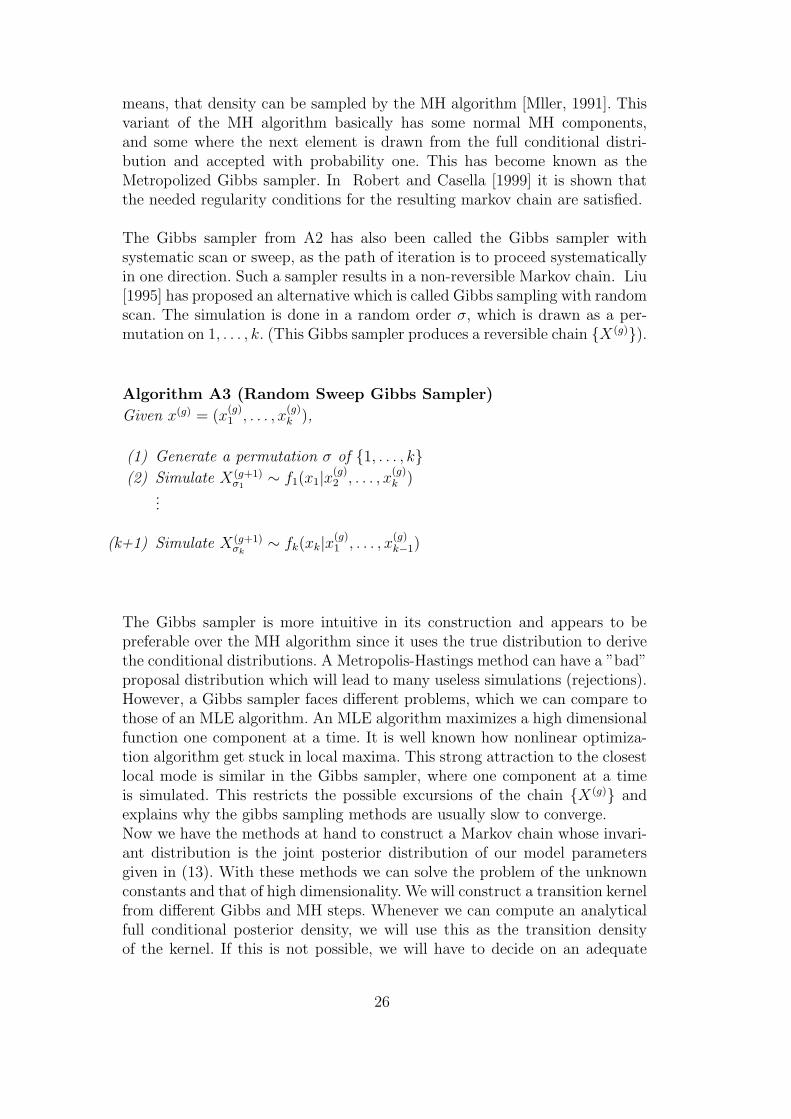
The Gibbs sampler from A2 has also been called the Gibbs sampler withsystematic scan or sweep, as the path of iteration is to proceed systematicallyin one direction. Such a sampler results in a non-reversible Markov chain. Liu[1995] has proposed an alternative which is called Gibbs sampling with randomscan. The simulation is done in a random order σ, which is drawn as a per-mutation on 1, . . . , k. (This Gibbs sampler produces a reversible chain X(g)).
Algorithm A3 (Random Sweep Gibbs Sampler)
Given x(g) = (x(g)1 , . . . , x
(g)k ),
(1) Generate a permutation σ of 1, . . . , k(2) Simulate X(g+1)
σ1∼ f1(x1|x(g)
2 , . . . , x(g)k )
...
(k+1) Simulate X(g+1)σk
∼ fk(xk|x(g)1 , . . . , x
(g)k−1)
The Gibbs sampler is more intuitive in its construction and appears to bepreferable over the MH algorithm since it uses the true distribution to derivethe conditional distributions. A Metropolis-Hastings method can have a ”bad”proposal distribution which will lead to many useless simulations (rejections).However, a Gibbs sampler faces different problems, which we can compare tothose of an MLE algorithm. An MLE algorithm maximizes a high dimensionalfunction one component at a time. It is well known how nonlinear optimiza-tion algorithm get stuck in local maxima. This strong attraction to the closestlocal mode is similar in the Gibbs sampler, where one component at a timeis simulated. This restricts the possible excursions of the chain X(g) andexplains why the gibbs sampling methods are usually slow to converge.Now we have the methods at hand to construct a Markov chain whose invari-ant distribution is the joint posterior distribution of our model parametersgiven in (13). With these methods we can solve the problem of the unknownconstants and that of high dimensionality. We will construct a transition kernelfrom different Gibbs and MH steps. Whenever we can compute an analyticalfull conditional posterior density, we will use this as the transition densityof the kernel. If this is not possible, we will have to decide on an adequate
26
proposal distribution.
In the next section we give a qualitative overview about how MCMC methodshave been used to estimate ARMA and GARCH models before we derive ourestimation procedure in section 5
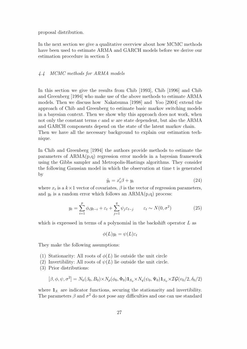
4.4 MCMC methods for ARMA models
In this section we give the results from Chib [1993], Chib [1996] and Chiband Greenberg [1994] who make use of the above methods to estimate ARMAmodels. Then we discuss how Nakatsuma [1998] and Yoo [2004] extend theapproach of Chib and Greenberg to estimate basic markov switching modelsin a bayesian context. Then we show why this approach does not work, whennot only the constant terms c and w are state dependent, but also the ARMAand GARCH components depend on the state of the latent markov chain.Then we have all the necessary background to explain our estimation tech-nique.
In Chib and Greenberg [1994] the authors provide methods to estimate theparameters of ARMA(p,q) regression error models in a bayesian frameworkusing the Gibbs sampler and Metropolis-Hastings algorithms. They considerthe following Gaussian model in which the observation at time t is generatedby
yt = x′tβ + yt (24)
where xt is a k×1 vector of covariates, β is the vector of regression parameters,and yt is a random error which follows an ARMA(p,q) process:
yt =p∑
i=1
φiyt−i + εt +q∑
j=1
ψjεt−j εt ∼ N(0, σ2) (25)
which is expressed in terms of a polynomial in the backshift operator L as
φ(L)yt = ψ(L)εt
They make the following assumptions:
(1) Stationarity: All roots of φ(L) lie outside the unit circle(2) Invertibility: All roots of ψ(L) lie outside the unit circle.(3) Prior distributions:
where 1S. are indicator functions, securing the stationarity and invertibility.The parameters β and σ2 do not pose any difficulties and one can use standard
27
results from the bayesian literature to arrive at analytical posterior distribu-tions. These are the Normal and Inverse Gamma respectively, since the priorsare conjugate 2 .
This is different for φ and ψ. The posterior density can only be derived up toa constant so that these vectors have to be drawn in a MH-step.A novelty in their article is the way in which they recursively transform themodel equations to diagonalize the covariance matrix of the errors yt. Thisresults in a very ”compact” expression for the unnormalized posterior density.This expression is not only compact, it yields a formulation of the covariancematrix for the parameter vectors φ and ψ, which are p and q dimensional. Theycan thus be drawn and tried in a single Metropolis-Hastings step instead ofdrawing each φi and ψj individually. This can be a desirable feature, since thecomputation of the acceptance probability in the MH algorithm is based onthe likelihood and can become very intensive. If the parameters are drawn inindividual steps, the product of the MH-kernels would account for the corre-lation between them, but the likelihood would have to be evaluated p+q times.
Then they construct a Markov chain from what some call a hybrid Gibbs-MHprocedure. β and σ2 are drawn from their analytical posterior distributionwhereas φ and ψ are generated by an MH step. For the MH step they exploitthe knowledge about the posterior distribution, expressed through the unnor-malized density (as we pointed out in subsection 4.2.2).They also prove that the conditions of proposition 4.3 are satisfied.
There does not seem to be much clarity in the literature, when an algorithmthat constructs a Markov chain based on the product of kernels principleis to be called a Gibbs-MH algorithm, a hybrid Gibbs-MH procedure or aMetropolized Gibbs sampler. In Chib and Greenberg [1995] the authors criti-cize the expression of Metropolized-Gibbs sampler, since Hastings introducedthe idea of drawing ”blocks at-a-time” much earlier. When we compared theGibbs sampler to the MH algorithm, we could see that the Gibbs sampler isindeed a special case of the ”block-at-a-time” algorithm where the proposaldistribution is the posterior distribution and the difference is that the accep-tance probability is set to one. Since the MH chain was, by construction, re-versible, we can see how this reversibility might be lost through a Gibbs kernel.
We will refer to a Gibbs step, when we draw from an analytically derivedposterior distribution and always accept the value. We refer to an MH step,when we draw from a proposal distribution and accept the value according to
2 These results correspond to table 1; note that the Inverse Gamma distributionis the general form of a scaled Inverse Chi Square distribution. They choose toformulate it in terms of the Inverse Gamma whereas we will prefer the form of ascaled inverse Chi Square distribution in later sections
28
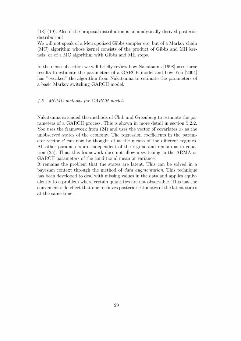
(18)-(19). Also if the proposal distribution is an analytically derived posteriordistribution!We will not speak of a Metropolized Gibbs sampler etc, but of a Markov chain(MC) algorithm whose kernel consists of the product of Gibbs and MH ker-nels, or of a MC algorithm with Gibbs and MH steps.
In the next subsection we will briefly review how Nakatsuma [1998] uses theseresults to estimate the parameters of a GARCH model and how Yoo [2004]has ”tweaked” the algorithm from Nakatsuma to estimate the parameters ofa basic Markov switching GARCH model.
4.5 MCMC methods for GARCH models
Nakatsuma extended the methods of Chib and Greenberg to estimate the pa-rameters of a GARCH process. This is shown in more detail in section 5.2.2.Yoo uses the framework from (24) and uses the vector of covariates xt as theunobserved states of the economy. The regression coefficients in the param-eter vector β can now be thought of as the means of the different regimes.All other parameters are independent of the regime and remain as in equa-tion (25). Thus, this framework does not allow a switching in the ARMA orGARCH parameters of the conditional mean or variance.It remains the problem that the states are latent. This can be solved in abayesian context through the method of data augmentation. This techniquehas been developed to deal with missing values in the data and applies equiv-alently to a problem where certain quantities are not observable. This has theconvenient side-effect that one retrieves posterior estimates of the latent statesat the same time.
29
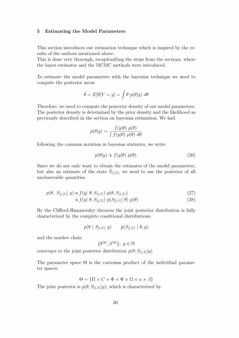
5 Estimating the Model Parameters
This section introduces our estimation technique which is inspired by the re-sults of the authors mentioned above.This is done very thorough, recapitualting the steps from the sections, wherethe bayes estimator and the MCMC methods were introduced.
To estimate the model parameters with the bayesian technique we need tocompute the posterior mean
θ = E[θ|Y = y] =∫
θ p(θ|y) dθ
Therefore, we need to compute the posterior density of our model parameters.The posterior density is determined by the prior density and the likelihood aspreviously described in the section on bayesian estimation. We had
p(θ|y) =f(y|θ) p(θ)∫f(y|θ) p(θ) dθ
following the common notation in bayesian statistics, we write
p(θ|y) ∝ f(y|θ) p(θ). (26)
Since we do not only want to obtain the estimates of the model parameters,but also an estimate of the state S[1,T ], we need to use the posterior of allunobservable quantities
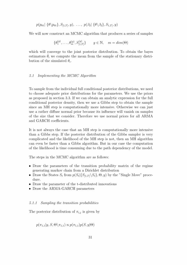
We will now construct an MCMC algorithm that produces a series of samples
θ(g)1 , . . . , θ(g)
m , S(g)[1,T ] g ∈ N, m = dim(Θ)
which will converge to the joint posterior distribution. To obtain the bayesestimators θi we compute the mean from the sample of the stationary distri-bution of the simulated θi.
5.1 Implementing the MCMC Algorithm
To sample from the individual full conditional posterior distributions, we needto choose adequate prior distributions for the parameters. We use the priorsas proposed in section 3.3. If we can obtain an analytic expression for the fullconditional posterior density, then we use a Gibbs step to obtain the samplesince an MH step is computationally more intensive. Otherwise we can justuse a rather diffuse normal prior because its influence will vanish on samplesof the size that we consider. Therefore we use normal priors for all ARMAand GARCH coefficients.
It is not always the case that an MH step is computationally more intensivethan a Gibbs step. If the posterior distribution of the Gibbs sampler is verycomplicated and the likelihood of the MH step is not, then an MH algorithmcan even be faster than a Gibbs algorithm. But in our case the computationof the likelihood is time consuming due to the path dependency of the model.
The steps in the MCMC algorithm are as follows:
• Draw the parameters of the transition probability matrix of the regimegenerating markov chain from a Dirichlet distribution
• Draw the States St from p(St|S[1,T ]\St, Θ, y) by the ”Single Move” proce-dure.
• Draw the parameter of the t-distributed innovations• Draw the ARMA-GARCH parameters
5.1.1 Sampling the transition probabilities
The posterior distribution of πi,j is given by
p(π1,1|y, S, Θ\π1,1)∝ p(π1,1)p(S, y|Θ)
31
Since St is independent of y, this is
p(π1,1|y, S, Θ\π1,1) ∝ p(π1,1)p(S|Θ)
Let ηi,j be the cumulated number of transitions from state i to state j in the
current sample S(g)[1,T ]. Then we can write this as:
p(S|Θ) =T∏
t=1
p(St+1|St, Θ) (29)
= (π1,1)η1,1(π1,2)
η1,2(π2,2)η2,2(π2,1)
η2,1 (30)
= (π1,1)η1,1(1− π1,1)
η1,2(π2,2)η2,2(1− π2,2)
η2,1
This has the form of a beta density. The conjugate prior is therefore a betadistribution with the hyperparameters h1,1, h1,2, h2,2 and h2,1. The posteriordistribution becomes:
p(π1,1|y, S, Θ\π1,1)∝ p(π1,1)p(S|Θ)
∝ (π1,1)h1,1−1(1− π1,1)
h1,2−1(π1,1)η1,1(1− π1,1)
η1,2
∝ (π1,1)η1,1+h1,1−1(1− π1,1)
η1,2+h1,2−1
Up to a constant this is the Beta density function. Therefore we sample πi,j
in a Gibbs sampling step from the following Beta distribution:
π1,1|S[1,T ]∼Beta(h1,1 + η1,1, h1,2 + η1,2)
π2,2|S[1,T ]∼Beta(h2,2 + η2,2, h2,1 + η2,1)
Higher dimensions of the chain:(29) would become
p(S|Θ) = (π1,1)η1,1(π1,2)
η1,2 . . . (π1,S)1,S · (π2,1)η2,1 . . .
for each row of Π, πs = (πs,1, . . . , πs,S), this is proportional to the densityfrom a Dirichlet distribution. A conjugate prior would thus be a Dirichletdistribution with the hyperparameters αs = (αs,1, . . . , αs,S)′:
f(x|α) =1
B(α)
k∏
i=1
xαi−1i B(α) =
∏ki=1 Γ(αi)
Γ(∑k
i=1 αi)
The posterior is then again a Dirichlet distribution with the parameters α+η.We therefore obtain a sample of the transition probabilities from state s to allothers by generating a draw from
In the next step, we need to obtain a sample of the states. We will followthe single move scheme suggested by Carlin et al. [1992].
5.1.2 Sampling S[1,T ]
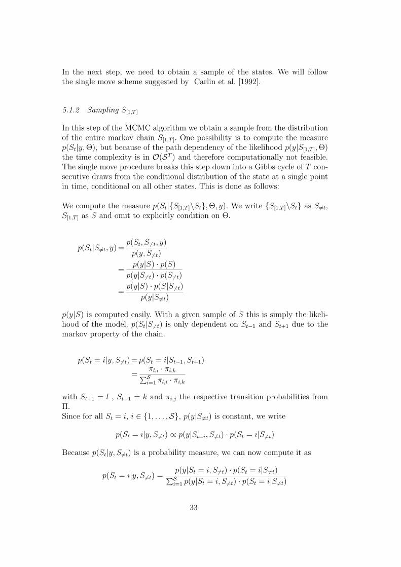
In this step of the MCMC algorithm we obtain a sample from the distributionof the entire markov chain S[1,T ]. One possibility is to compute the measurep(St|y, Θ), but because of the path dependency of the likelihood p(y|S[1,T ], Θ)the time complexity is in O(ST ) and therefore computationally not feasible.The single move procedure breaks this step down into a Gibbs cycle of T con-secutive draws from the conditional distribution of the state at a single pointin time, conditional on all other states. This is done as follows:
We compute the measure p(St|S[1,T ]\St, Θ, y). We write S[1,T ]\St as S 6=t,S[1,T ] as S and omit to explicitly condition on Θ.
p(St|S 6=t, y) =p(St, S 6=t, y)
p(y, S 6=t)
=p(y|S) · p(S)
p(y|S 6=t) · p(S 6=t)
=p(y|S) · p(S|S 6=t)
p(y|S6=t)
p(y|S) is computed easily. With a given sample of S this is simply the likeli-hood of the model. p(St|S 6=t) is only dependent on St−1 and St+1 due to themarkov property of the chain.
p(St = i|y, S 6=t) = p(St = i|St−1, St+1)
=πl,i · πi,k∑S
i=1 πl,i · πi,k
with St−1 = l , St+1 = k and πi,j the respective transition probabilities fromΠ.Since for all St = i, i ∈ 1, . . . ,S, p(y|S 6=t) is constant, we write
p(St = i|y, S 6=t) ∝ p(y|St=i, S 6=t) · p(St = i|S 6=t)
Because p(St|y, S 6=t) is a probability measure, we can now compute it as
p(St = i|y, S 6=t) =p(y|St = i, S 6=t) · p(St = i|S 6=t)∑S
i=1 p(y|St = i, S 6=t) · p(St = i|S 6=t)
33
One sample of S[1,T ] is thus obtained by cycling through these steps:For each t ∈ 1, . . . , T, starting with t = 1:
• Compute the distribution p(St = i|S 6=t, y) on 1, . . . ,S.• Draw St from this distribution.• Update S[1,T ] with this value.
This is also a Gibbs sampler with systematic scan.
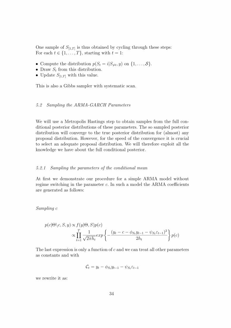
5.2 Sampling the ARMA-GARCH Parameters
We will use a Metropolis Hastings step to obtain samples from the full con-ditional posterior distributions of these parameters. The so sampled posteriordistribution will converge to the true posterior distribution for (almost) anyproposal distribution. However, for the speed of the convergence it is crucialto select an adequate proposal distribution. We will therefore exploit all theknowledge we have about the full conditional posterior.
5.2.1 Sampling the parameters of the conditional mean
At first we demonstrate our procedure for a simple ARMA model withoutregime switching in the parameter c. In such a model the ARMA coefficientsare generated as follows:
Sampling c
p(c|Θ\c, S, y)∝ f(y|Θ, S)p(c)
∝T∏
t=1
1√2πht
exp
−(yt − c− φStyt−1 − ψStεt−1)
2
2ht
p(c)
The last expression is only a function of c and we can treat all other parametersas constants and with
Ct = yt − φStyt−1 − ψStεt−1
we rewrite it as:
34
T∏
t=1
1√2πht
exp
−(Ct − c)2
2ht
p(c) =
T∏
t=1
1√2πht
exp
−C
2t − 2Ct · c + c2
2ht
p(c)
∝ exp
∑Tt=1 C2
t
2ht
· exp
T∑
t=1
−2Ct · c + c2
2ht
p(c)
∝ exp
∑Tt=1 C2
t
2ht
· exp
c ·
T∑
t=1
−Ct
ht
+ c2T∑
t=1
1
2ht
p(c)
This has the form of a normal density with
σ−2 =T∑
t=1
1
ht
µ =T∑
t=1
Ct
ht
·(
T∑
t=1
1
ht
)−1
As the proposal distribution we choose N(µc, σ2c ) with
µc =T∑
t=1
yt − φStyt−1 − ψStεt−1
ht
·(
T∑
t=1
1
ht
)−1
σ−2c =
T∑
t=1
1
ht
For the other parameters we can proceed in a similar fashion. Next we in-troduce regime switching only into the mean and then outline the completealgorithm for the full model.The model is
Even though we cannot observe the state St in reality, the MCMC algorithmprovides us with a sample S[1,T ] which we simply plug into the above formula.And following the previous steps we arrive at:
p(c1|Θ\c1, S, y) ∝ exp
c1
T∑
t=1
−Ct1[St=1]
ht
+ c21
T∑
t=1
1[St=1]
2ht
The proposal Distribution therefore is N(µc1 , σ2c1
) with
µc1 =T∑
t=1
1[St=1]yt − 1[St=1]φ1yt−1 − 1[St=1]ψ1εt−1
ht
·(
T∑
t=1
1[St=1]
ht
)−1
35
σ−2c1
=T∑
t=1
1[St=1]
ht
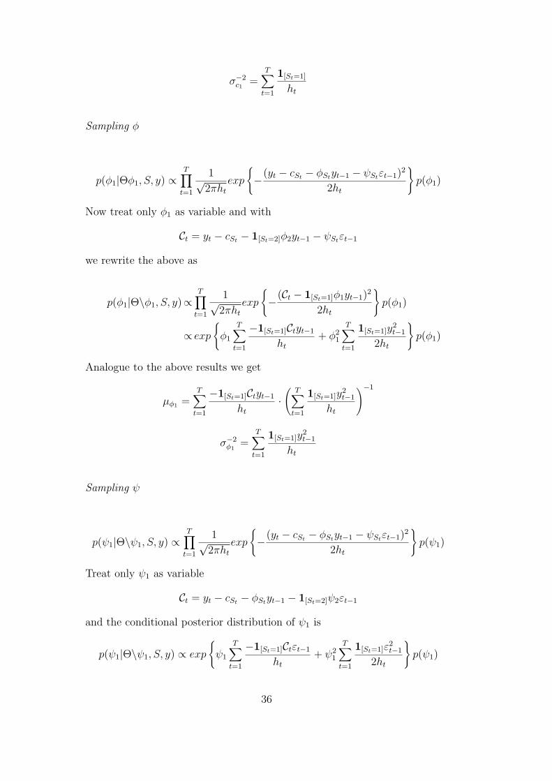
Sampling φ
p(φ1|Θφ1, S, y) ∝T∏
t=1
1√2πht
exp
−(yt − cSt − φStyt−1 − ψStεt−1)
2
2ht
p(φ1)
Now treat only φ1 as variable and with
Ct = yt − cSt − 1[St=2]φ2yt−1 − ψStεt−1
we rewrite the above as
p(φ1|Θ\φ1, S, y)∝T∏
t=1
1√2πht
exp
−(Ct − 1[St=1]φ1yt−1)
2
2ht
p(φ1)
∝ exp
φ1
T∑
t=1
−1[St=1]Ctyt−1
ht
+ φ21
T∑
t=1
1[St=1]y2t−1
2ht
p(φ1)
Analogue to the above results we get
µφ1 =T∑
t=1
−1[St=1]Ctyt−1
ht
·(
T∑
t=1
1[St=1]y2t−1
ht
)−1
σ−2φ1
=T∑
t=1
1[St=1]y2t−1
ht
Sampling ψ
p(ψ1|Θ\ψ1, S, y) ∝T∏
t=1
1√2πht
exp
−(yt − cSt − φStyt−1 − ψStεt−1)
2
2ht
p(ψ1)
Treat only ψ1 as variable
Ct = yt − cSt − φStyt−1 − 1[St=2]ψ2εt−1
and the conditional posterior distribution of ψ1 is
p(ψ1|Θ\ψ1, S, y) ∝ exp
ψ1
T∑
t=1
−1[St=1]Ctεt−1
ht
+ ψ21
T∑
t=1
1[St=1]ε2t−1
2ht
p(ψ1)
36
Therefore we choose N(µψ1 , σ2ψ1
) as the proposal distribution with
µψ1 =T∑
t=1
−1[St=1]Ctεt−1
ht
·(
T∑
t=1
1[St=1]ε2t−1
ht
)−1
σ−2ψ1
=T∑
t=1
1[St=1]ε2t−1
ht
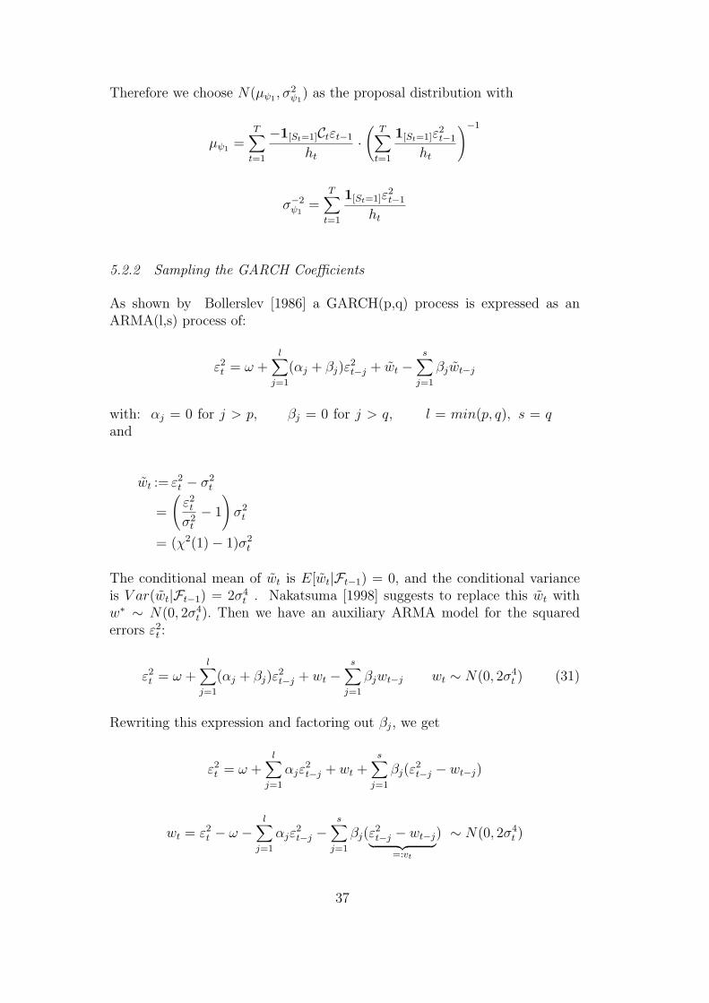
5.2.2 Sampling the GARCH Coefficients
As shown by Bollerslev [1986] a GARCH(p,q) process is expressed as anARMA(l,s) process of:
ε2t = ω +
l∑
j=1
(αj + βj)ε2t−j + wt −
s∑
j=1
βjwt−j
with: αj = 0 for j > p, βj = 0 for j > q, l = min(p, q), s = qand
wt := ε2t − σ2
t
=
(ε2
t
σ2t
− 1
)σ2
t
= (χ2(1)− 1)σ2t
The conditional mean of wt is E[wt|Ft−1) = 0, and the conditional varianceis V ar(wt|Ft−1) = 2σ4
t . Nakatsuma [1998] suggests to replace this wt withw∗ ∼ N(0, 2σ4
t ). Then we have an auxiliary ARMA model for the squarederrors ε2
t :
ε2t = ω +
l∑
j=1
(αj + βj)ε2t−j + wt −
s∑
j=1
βjwt−j wt ∼ N(0, 2σ4t ) (31)
Rewriting this expression and factoring out βj, we get
ε2t = ω +
l∑
j=1
αjε2t−j + wt +
s∑
j=1
βj(ε2t−j − wt−j)
wt = ε2t − ω −
l∑
j=1
αjε2t−j −
s∑
j=1
βj(ε2t−j − wt−j︸ ︷︷ ︸
=:vt
) ∼ N(0, 2σ4t )
37
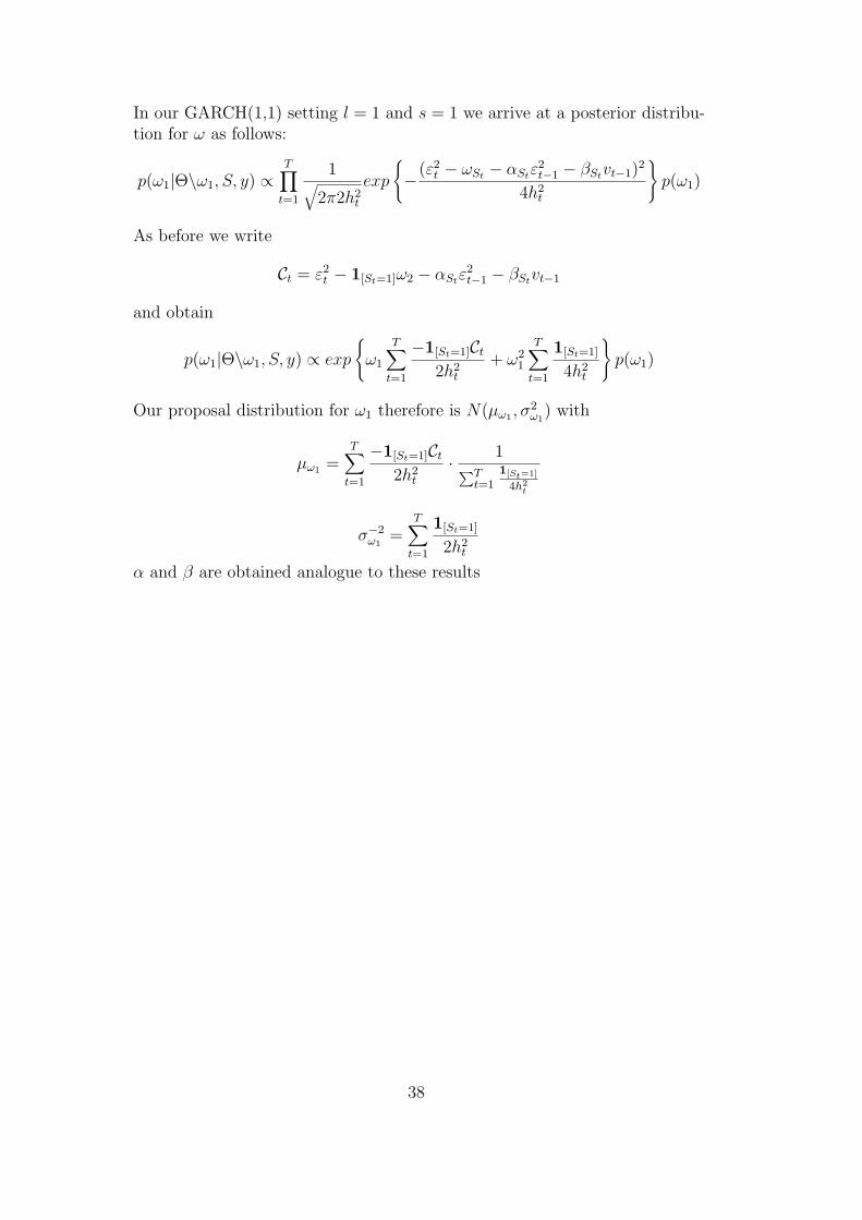
In our GARCH(1,1) setting l = 1 and s = 1 we arrive at a posterior distribu-tion for ω as follows:
p(ω1|Θ\ω1, S, y) ∝T∏
t=1
1√2π2h2
t
exp
−(ε2
t − ωSt − αStε2t−1 − βStvt−1)
2
4h2t
p(ω1)
As before we write
Ct = ε2t − 1[St=1]ω2 − αStε
2t−1 − βStvt−1
and obtain
p(ω1|Θ\ω1, S, y) ∝ exp
ω1
T∑
t=1
−1[St=1]Ct
2h2t
+ ω21
T∑
t=1
1[St=1]
4h2t
p(ω1)
Our proposal distribution for ω1 therefore is N(µω1 , σ2ω1
) with
µω1 =T∑
t=1
−1[St=1]Ct
2h2t
· 1∑T
t=11[St=1]
4h2t
σ−2ω1
=T∑
t=1
1[St=1]
2h2t
α and β are obtained analogue to these results
38
5.3 Estimating the parameters of the t-distributed innovations
In the model where the innovations are student t-distributed, the algorithmchanges slightly. The MH-steps essentially stay the same, but we will adjustthe proposal distribution. We also have to estimate the degree of freedom pa-rameter vSt .First let us consider the posterior distribution of the degree of freedom param-eter v. Again the model can be specified in several ways, one possibility is tomodel the innovations independent of the states, that is to say, there is onlyone v for all t. Or this parameter could also be chosen to be state dependent.To start with we will consider the former case of a regime independent degreeof freedom parameter. It will then be straight forward to extend the approach.
5.3.1 Sampling v
We follow Jacquier et al. [2003] and choose a discrete flat prior for v, whereasGeweke [1993] uses a continous prior to estimate the degree of freedom instudent-t linear models. The posterior distribution of v is proportional to theproduct of t distribution ordinates:
p(v|Θ\v, S, y)∝ p(v)p(y|Θ, S)
∝T∏
t=1
Γ(v+12
)√vπ Γ(v
2)(1 +
e2t
htv)−( v+1
2)
where
et = yt −r∑
i=1
φi(St)yt−i −m∑
i=1
ψi(St)εt−i
Theoretically v is in N+, but we choose a flat prior on 3, . . . , 40. The poste-rior distribution can then be calculated analytically as follows:Let
p(v|Θ\v, S, y) =T∏
t=1
Γ(v+12
)√vπ Γ(v
2)(1 +
e2t
htv)−( v+1
2) (32)
Then for p(v|Θ\v, S, y) with a flat prior on 3, . . . , 40, p(v) = 137
, we get:
p(v|Θ\v, S, y) =p(v|Θ\v, S, y)
∑40i=3 p(i|Θ\i, S, y)
· 1
37
Truncating the interval of v on 3, . . . , 40 will not result in inaccuracies aslong as the sampled values v(g) do not touch the boundaries. We will onlychoose to model data with a t-distribution if the degree of freedom is sig-nificantly smaller than 30. Above 30 it is common in statistical literature to
39
approximate the t-distribution with the normal since they are very close.
5.3.2 Proposal Distributions
With normally distributed innovations we were able to find a good proposaldistribution analytically. It is also common in the literature on MCMC al-gorithms to choose a proposal distribution who’s moments are obtain by aMaximum Likelihood estimate. This is legitimate even though it appears asone is mixing up the different inferential approaches. The ML estimates merelyserve as proxies for the means and the variances of the proposal distributions.In fact the parameters µ and σ as they were computed in section (5.2) corre-spond exactly to the ML estimates of the mean and variance of the conditionaldistribution.The scheme we used to obtain the paramters for the normal do not work fort-distributed innovations, where we end up with a nonlinear expression. TheML estimates are also obtained from a nonlinear equation and in practice theyare calculated numerically.
In our bayesian context we can circumvent this inconvenience due to the factthat for Student’s t-distribution, there exists a hidden mixture representa-tion through the normal distribution. Since p(x|θ) is the mixture of a normaldistribution and an inverse gamma distribution:
x|z∼N(θ, zσ2),
z−1∼Gamma(v
2,v
2).
This is a well known trick in the bayesian literature, see for example Robert[1994].We can now rewrite our model as
yt = cSt +r∑
i=1
φi(St) · yt−i + ηt +m∑
j=1
ψj(St) · ηt−j (33a)
ht = ωSt +p∑
i=1
αi(St) · η2t−i +
q∑
j=1
βj(St) · ht−j (33b)
ηt =√
ht · ηt (33c)
ηt =√
λt · ut ∼ t(v) (33d)
ut∼N(0, 1) (33e)
λt∼IG(v
2,v
2) (33f)
40
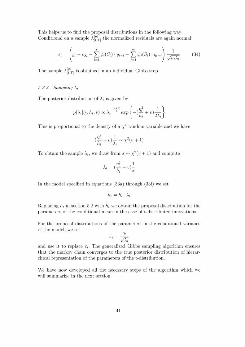
This helps us to find the proposal distributions in the following way:Conditional on a sample λ
(g)[1,T ] the normalized residuals are again normal:
εt =
yt − cSt −
r∑
i=1
φi(St) · yt−i −m∑
j=1
ψj(St) · ηt−j
1√
htλt
(34)
The sample λ(g)[1,T ] is obtained in an individual Gibbs step.
5.3.3 Sampling λt
The posterior distribution of λt is given by
p(λt|ηt, ht, v) ∝ λ− (v+3)
2t exp
−(
η2t
ht
+ v)1
2λt
This is proportional to the density of a χ2 random variable and we have
(η2
t
ht
+ v)1
λt
∼ χ2(v + 1)
To obtain the sample λt, we draw from x ∼ χ2(v + 1) and compute
λt = (η2
t
ht
+ v)1
x
In the model specified in equations (33a) through (33f) we set
ht = ht · λt
Replacing ht in section 5.2 with ht we obtain the proposal distribution for theparameters of the conditional mean in the case of t-distributed innovations.
For the proposal distributions of the parameters in the conditional varianceof the model, we set
εt =ηt√λt
and use it to replace εt. The generalized Gibbs sampling algorithm ensuresthat the markov chain converges to the true posterior distribution of hierar-chical representation of the parameters of the t-distribution.
We have now developed all the necessary steps of the algorithm which wewill summarize in the next section.
41
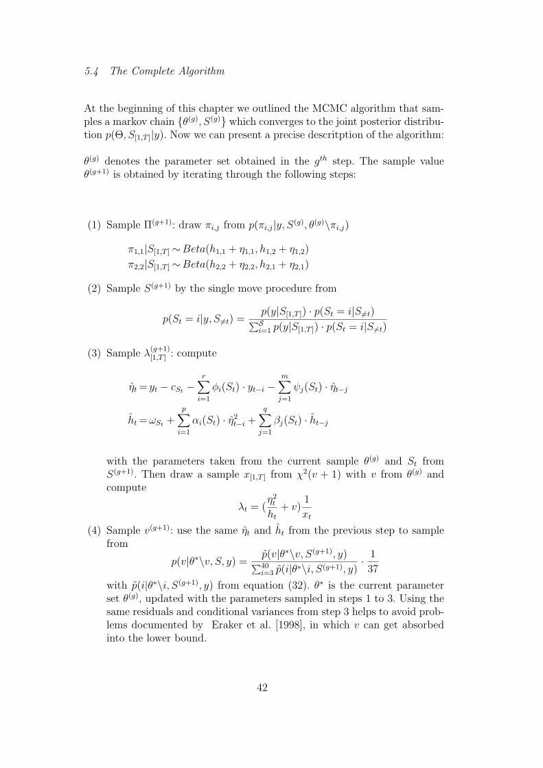
5.4 The Complete Algorithm
At the beginning of this chapter we outlined the MCMC algorithm that sam-ples a markov chain θ(g), S(g) which converges to the joint posterior distribu-tion p(Θ, S[1,T ]|y). Now we can present a precise descritption of the algorithm:
θ(g) denotes the parameter set obtained in the gth step. The sample valueθ(g+1) is obtained by iterating through the following steps:
(1) Sample Π(g+1): draw πi,j from p(πi,j|y, S(g), θ(g)\πi,j)
π1,1|S[1,T ]∼Beta(h1,1 + η1,1, h1,2 + η1,2)
π2,2|S[1,T ]∼Beta(h2,2 + η2,2, h2,1 + η2,1)
(2) Sample S(g+1) by the single move procedure from
with the parameters taken from the current sample θ(g) and St fromS(g+1). Then draw a sample x[1,T ] from χ2(v + 1) with v from θ(g) andcompute
λt = (η2
t
ht
+ v)1
xt
(4) Sample v(g+1): use the same ηt and ht from the previous step to samplefrom
p(v|θ∗\v, S, y) =p(v|θ∗\v, S(g+1), y)
∑40i=3 p(i|θ∗\i, S(g+1), y)
· 1
37
with p(i|θ∗\i, S(g+1), y) from equation (32). θ∗ is the current parameterset θ(g), updated with the parameters sampled in steps 1 to 3. Using thesame residuals and conditional variances from step 3 helps to avoid prob-lems documented by Eraker et al. [1998], in which v can get absorbedinto the lower bound.
42
(5) Cycle through the ARMA-GARCH parameters. For each parameter drawfrom the respective proposal distribution by the scheme outlined above.The candidate is then tried in a Metropolis Hastings step according tosection 4.2 and either accepted or rejected.Let ϑ denote the proposed parameter value. We update θ∗ with this valueand refer to this parameter set as θ. We accept θ as the new θ∗ withprobability
αMH(θ∗, θ) = min
p(θ| y, S(g+1))
p(θ∗| y, S(g+1))
/ g(θ)
g(θ∗), 1
where p(θ| y, S(g+1)) is the likelihood of the data y and the current sampleS(g+1), calculated with the parameter set θ. g(.) is the respective proposaldensity. This is done for all parameters of the ARMA-GARCH specifica-tion. Finally we have obtained the new sample θ(g+1), S(g+1).
5.4.1 Variations of the Algorithm
As discussed in section 4.3 there are several variations of the MH- and GibbsSampling algorithm. These differ in their performance especially when it comesto sample the ARMA-GARCH parameters. For the different regimes these pa-rameters are highly correlated and their generation is computationally inten-sive. Chib and Greenberg report that they could increase the performance ofMH algorithms when highly correlated parameters were sampled in a block.We can confirm this observation. Especially for the conditional mean we ob-served that the chain converged much faster to its stationary distribution.Even though more proposals were rejected, the chain moved around morefreely in the parameter space and thereby explored the shape of the posteriorfaster because it did not get stuck in certain regions for too long. We alsofound the algorithm proposed by Liu [1995] to be beneficial in this respect.
Most numerical implementations of parameter estimation algorithms performquite well, if the data is well behaved and fits well. The more interesting casesare the ones, were the parameters of a model are at the border of the respec-tive parameter space. For ARMA-GARCH processes such a ’stress’ situationarises, when the process is close to being integrated. We simulated a station-ary MS-ARMA-GARCH model with the sum of the GARCH parameters beingclose to unity. The acceptance rates of some parameters dropped to about tenpercent, resulting in a slow convergence of the Markov chain. Here we foundthat a specification of the algorithm presented in 5.4, were each parameter wastried separately in an MH step could increase the acceptance rate. Such a lowacceptance rate can create problems with the convergence of the estimatesof the regime process. Since the Gibbs step for the states is the most timeconsuming, we only do this every 10 iterations of the algorithm, allowing the
43
ARMA-GARCH parameters to explore their changed posterior distributions.We argued above, that a drop in the acceptance rate does not necessarily havea negative effect as long as the chain explores the whole parameter space bet-ter. But if the ARMA-GARCH parameters get only updated once in betweento samples of the states, this can slow down the convergence considerably.
Another problem, that arises in the case, when either the conditional mean orvariance is close to being integrated, is the choice of the proposal distribution.Say for example that β1(1) = 0.95, then the normal approximation for wt isvery questionable and the proposed mean µβ1 will often be greater than one.This leads to an extremely high rejection of the proposed value. Since we wantto impose stationarity, we do not accept βi’s that are equal or greater thanone. If µbetai
should be greater than one, we will set µbetai= β(g). This has
proven to be very useful when we estimated simulated data with one βi beingclose to one.
5.5 Estimating Hamilton’s ’94 model with this algorithm
For the purpose of comparison, we will also estimate a variant of the modelproposed in Hamilton and Susmel [1994]. With the method developed in thissection, it is not a big step to compute the estimators for M2. We will deviateslightly from Hamilton’s proposal and formulate the model as
Model M5 (Modified Hamilton ’94) The latent state governing the evo-lution of the model parameters is again assumed to follow an S dimensionaltime discrete Markov chain whose transition matrix is given through (1). Theconditional mean of the time series yt is as in (2a)
yt = cSt +r∑
i=1
φi(St) · yt−i + εt +m∑
j=1
ψj(St) · εt−j
ht = w +q∑
i=1
αi · εt−i +p∑
j=1
βj · ht−j
εt =√
gSt ·√
ht · ut
ut∼N(0, 1)
The mean is as in model M4 and the conditional variance is an amplifiedGARCH process. The main difference between model M2 and M4 is the spec-ification of the variance. The other parameters of the model can be estimatedthrough a straightforward application of the methods shown in the previoussections. Therefore we will now discuss how the amplifying parameter gSt can
44
be estimated within our MCMC setting.
The likelihood f(θ|y, S[1,T ]) is given through
f(θ|y, S[1,T ]) =∏
t1∈I1
1√2πg1ht
exp
− ε2
t1
2g1htt1
×. . .× ∏
tS∈IS
1√2πgSht
exp
− ε2
ts
2gShts
where Is is the index set containing all points in time when St = s. It is easyto see that for a certain gs the likelihood of gs is proportional to
f(gs|θ\gs, y, S[1,T ])∝∏
ts∈Is
1√2πht
g−12 exp
−ε2
t /(2ht)
gs
∝ g−Ns/2s exp
−
1
gs
∑
t∈Is
ε2t
2ht
where Ns = card(Is). This has the form of an Inverse Gamma density, whichis
f(x|α, β) =βα
Γ(α)x−α−1exp
−β
x
with shape parameter α and scale parameter β. Therefore a conjugate priorp(gs) is an inverse gamma distribution with the hyperparameters α0, β0. Theposterior distribution for gs would then be
f(gs|θ\gs, y, S[1,T ]) ∝ g−Ns/2exp
−
1
gs
∑
t∈Is
ε2t
2ht
· p(gs|α0, β0)
and hence
gs ∼ IG(1
2Ns + α0,
∑
t∈Is
ε2t
2ht
+ β0)
We specified the innovations ut as coming from a normal distribution. Wecould also let them be student t-distributed, in the estimation procedure wewould then simply have to apply the result from subsection 5.3.2.
45
6 Diagnosing Convergence
This section provides some words about how to check wether the markov chainof the MCMC algorithm has ’converged’. This can of course never be said forsure, but there are some visual indicators and some statistics that can be cal-culated.
Robert and Casella [1999] differentiate between three types of convergencecriteria. These differ in increasingly stringent conditions:
(1) Convergence to the Invariant DistributionThis criterion considers the convergence of the chain X(g) to the invariantdistribution f . However, f is only the limiting distribution of X(g) andinvariance is only an asymptotical property.
(2) Convergence of AveragesThis type considers the convergence of the empirical average
1
N
N∑
g=1
h(X(g))
to Ef [h(X)].(3) Convergence to iid Sampling
This convergence criterion measures how close a sample is to being iidand looks at the independence requirements for the simulated values.
We will be most concerned with the convergence of averages. Even if the initialvalues, x(0) are distributed according to f , the exploration of the support of fby the chain can be poor. This will depend heavily on the transition kernel,chosen in the MCMC algorithm. The purpose of the convergence assessementis therefore to determine whether the chain has scanned f to a satisfactorydegree. While the ergodic theorem guarantees the convergence theoretically,it is most relevant in a practical implementation to have a stopping rule. Thisrule would yield a minimal N which justifies the approximation of Ef [h(X)].
Robert and Casella provide a graphical method which is due to Yu and Myk-land [1998]. It is based on cumulative sums (CUSUM), where they plot thedifferences
DiN =
i∑
g=1
[h(X(g))− hN ], i = 1, 2, . . . , N (35)
where
hN =1
N
N∑
g=1
h(X(g)).
They derive a qualitative evaluation of the mixing speed of the chain and thecorrelation between the X(g)’s. When the mixing of the chain is high, the graph
46
of DiN is highly irregular and concentrated around zero. Slowly mixing chains
produce regular graphs with long excursions away from 0. The difficulty withthis method is, that it does not give any indications for unexplored regions ofthe chain. This is because the diagnose is only based on a single chain andone gets no idea of the regions that have not been seen.
47
7 Estimation Results
7.1 Performance of the Estimator on Simulated Data
We simulate different parameterizations of the model and take a closer lookat the posterior statistics. These results can then be compared to the onesretrieved on real data and help to judge the performance of the estimator andits convergence.We commence by assessing the quality of the estimates on single regime pro-cesses and compare them to the respective ML estimates. Then we comparethe results that we achieved with our estimation methodology to results previ-ously reported in the literature. Bauwens and Lubrano [1998] derive a GriddyGibbs sampler to estimate the parameters of simple GARCH processes. Theirmain focus is directed to the performance of their method on small samples.This is the area where the ML methodology differs mainly from the bayesianapproach. On samples of about 100-150 data points the influence broughtabout by the choice of the prior distributional assumption clearly shows.Chib and Greenberg [1994] develop a hybrid mcmc method in which they useboth MH and Gibbs sampling steps to estimate processes with ARMA(p,q)errors. They too, consider small samples when they compare their estimatorsto the ML alternative.
For the results in table 2 we used a constant scaling factor for the varianceof the proposal distribution of 1.5. The proposal distribution was a Student-tdistribution with degree of freedom v(g). They use a flat prior for the degree
Table 2Posterior results by different methods for a Student-t-GARCH model on simulateddata.
of freedom parameter, which seems to result in a bias on such small samples.This influence seems to vanish on larger samples as we will see later. For theIS (Importance Sampling) algorithm they base their importance function ona Student-t density and fix the location parameter at the posterior mode.The scaling parameters were tuned experimentally. For the MH estimator (seeMH(1) in table 2) they use the same Student-t distribution as a proposal dis-tribution. The results that we achieve with our algorithm (MH(2)) compare
48
well to those of the other methods, if not better. This is however hard to de-termine on such a small sample.Even though we are less concerned with smaller samples, using their resultsas a benchmark for our estimation procedure underpins the correctness of ourapproach.
In table 2 we can see how different the results can be. Whereas Bauwensand Lubrano’s MH algorithm seems less capable on the small sample, ourspecification seems to produce the best result. This is due to the issues thatwe already addressed in section 4.2.2. The method of determining the loca-tion and scale parameters of the proposal distribution is critical for the MHalgorithm to explore the domain of the posterior distribution. Our algorithmprovides an automatic choice for the location parameter of the proposal dis-tribution which varies along the chain. It does also produce a value for thescale parameter (variance). Even though these values are produced using ourknowledge about the posterior distribution, this does not necessarily makethem the best choice. To see this we compared several choices of the variancescaling parameter.
The results from table 2 were found on a small sample of 150 data points.Our focus is on larger samples, where the influence of the information impliedby the prior distribution vanishes as we discussed in section 3.2.2. We willnow study the behavior of our estimator on larger samples and under moredifficult parameterizations.
Table 3 reports the results for the estimator on a simulated GARCH processwith 1500 data points. The estimates for w and β seem ”a bit off”. Runningthe algorithm on the same data set, with the proposal variance scaled by fac-tor 1.5, the results reported in table y are now very close to the true values.The parameters of the GARCH process were chosen to be rather moderate.That is, that they were not close to being integrated. As with a maximizationalgorithm, the performance of the MCMC methods could change, when thealgorithm operates close to the border of a constrained domain. To see howour algorithm reacts in such cases, we studied the results on parameteriza-tions where the sum α + β was in between 0.9 and 1. Especially for high β’sthe acceptance rate drops very fast, which makes it necessary to increase thenumber of iterations of the algorithm. Nevertheless, our algorithm did not get”stuck” at any point and we conclude that it is reliable.
Our algorithm produces the correct results on samples with normally dis-tributed innovations. Now we can examine its performance for student-t-distributed innovations. Here we found that with several parameterizationsthe degree of freedom parameter can be biased towards higher values. This
Table 3This table compares the performance of the algorithm with two different choices ofthe variance scaling parameter. The GARCH process that is estimated was simu-lated with normal innovations and had a length of 1500 data points. The MCMCchain was run 50000 iterations of which the first 10000 were discarded (burn intime). The variance scaling parameter was set to 1 and 1.5 respectively.
bias for v seems to be a problem in those cases where∑q
i=1 α +∑p
j=1 β isabout 0.9 or higher. For other parameterizations the estimates where againvery close to the true values, and exhibited small posterior standard devi-ations. The results presented in table 4 illustrate our findings for a specificsimulation. Here we can see that for α = 0.3 and β = 0.6 the true v is evenbelow the estimated 5% quantile. In the second panel we estimated a processwith the same GARCH parametrization but normal innovations and see thatthe true parameters are recovered very precisely.
We recall that the degree of freedom parameter is drawn from a closed form(full conditional) posterior distribution in a Gibbs step. In Robert and Casella[1999] the authors report, that a chain from a Gibbs sampler can be very slowto converge. A bias such as the one we observed can occur when the chaindoes not explore all modes of the parameter space and gets trapped in a cer-tain region. The speed of convergence can then be ameliorated by includingan additional MH step in the algorithm. This MH step helps to avoid gettingtrapped in certain regions and allows the chain to move around more freely inthe parameter space.
Having verified the performance of the algorithm on single regime processes,we can now examine the performance on simulated data from multi-regimeMarkov switching processes. In table 5 we see that the algorithm performswell, estimating the parameters of a Markov switching process. Again, thesum of the GARCH parameters is considerably smaller than 0.9. Although
50
Parameter True value θ σ Median 5% quant. 95% quant. AR
w 0.1 0.132 0.024 0.131 0.093 0.173 0.321
α 0.3 0.374 0.041 0.374 0.308 0.443 0.322
β 0.6 0.535 0.037 0.535 0.474 0.597 0.327
v 7 14.07 5.13 13 8 24
w 0.1 0.098 0.017 0.097 0.071 0.126 0.259
α 0.3 0.318 0.033 0.316 0.265 0.376 0.255
β 0.6 0.616 0.030 0.617 0.560 0.665 0.253
v 0
Table 4The simulated GARCH process spanned 1500 data points. The MCMC chain wasrun 50000 iterations of which the first 10000 were discarded (burn in time). Thevariance scaling parameter was set to 1.5 .
not depicted here, the estimates for the latent states reliably reproduced thetrue values.
Studying the performance on simulated data, we could verify the reliabilityof our procedure and can now move on to real data. In the next section weexamined data from the New York Stock exchange. The estimated GARCHparameters were in those ranges where we did not experience these problemsfor the degree of freedom. Therefore we did not implement a version of thealgorithm where the v was sampled in an MH-step.
7.2 Empirical Results
In this section we provide the estimation results of our model specification andmake an effort to compare them to other results reported in the literature.
In Hamilton and Susmel [1994], estimates of the parameters for model M2are reported and several different parameterizations are compared to eachother. The authors conclude that the t-SWARCH-L(3,2) specifications is themost appropriate model for that data. They assessed the suitability of theirmodel mainly through the forecasting properties. They observed that the sin-gle regime GARCH models implied a very high persistence, but did a worse
Table 5The simulated GARCH process spanned 1500 data points. The MCMC chain wasrun 50000 iterations of which the first 10000 were discarded (burn in time). Thevariance scaling parameter was set to 1.5 .
job forecasting the volatility than a simple constant variance model measuredby mean squared errors. This is counterintuitive, since if the variance was per-sistent, that would imply better forecasts with a model that accounts for thispersistence.
GARCH(1,1) models are generally outperforming low order ARCH(q) modelswhen it comes to forecasting the conditional variance. It is a more parsimo-nious approach to capture the autocorrelation structure of the process andis therefore often preferred over an ARCH(q) specification. For this reasonwe believe that regime switching processes should be modelled with switchingGARCH processes rather than low order ARCH processes. Also the condi-tional mean should be modelled as either a one state ARMA(r,m) process ora switching ARMA(r,m) process. If the autocorrelation structure of the meanprovides a better fit to the data, this will have positive repercussions on theestimates of the conditional variance as well.
We use the same data set to see if the our specification improves the model fit.We looked at the sample autocorrelation function (sample ACF) for the weeklyreturns and found that a simple AR(1) specification of the conditional meanseemed to be an unlikely candidate to capture this rather complex structure.We decided to start with the standard ARMA(1,1)-GARCH(1,1) model withgaussian innovations and fitted it to the data. In a first step we assessed thegoodness of fit through an examination of the sample ACF for the estimatedresiduals of the one day ahead forecasts. These exhibited significant autocor-relations in the mean at lag 1,3,6 and 8 at the 5 percent level. The sum ofthe estimates for the GARCH coefficients is close to unity, indicating that theprocess of the conditional variance could be integrated, hence the estimateswould be of no great value.
52
We therefore estimated the parameters of an ARMA(1,1)-GARCH(1,1) modelwith t-distributed innovations, which seemed to provide an adequate descrip-tion of the dependency structure, measured by the sample ACF of the esti-mated standardized residuals ut. When we examined the distributional shapeof these residuals we could see in a qqplot, that they did not seem to be asheavy tailed as implied by a student t-distribution as estimated. Except forthe one outlier produced by the crash in ’87.
The observed values of the sample ACF of the residuals were extremely small.This is caused by the extreme innovation of the crash in ’87. In this modelsuch an event would have to be regarded as an outlier. If we would not regardthis value as an outlier, this indicates that the data actually stems from adistribution that has much heavier tails. In fact such a model would not evenhave a variance nor a finite covariance. The autocorrelation as a measure fordependance is then not very meaningful. Never the less, we could truncate thedata set to exclude this extreme event, and then try to describe the depen-dency with the sample ACF. This gives us a proxy by which we can diagnosethe model fit of the rest of the data.
The sample ACF of the residuals of the truncated data set showed no sig-nificant autocorrelations. This indicates that the single regime ARMA mightbe enough to describe the mean of the weekly return series. In fact, as wefitted a two regime model of the mean, the results of the algorithm were veryunstable in the estimated states, also an indication of no significant switchingin the mean.
We then fitted an MS(1,2)-ARMA(1,1)-GARCH(1,1) specification of M4 tothe data. Compared to the single regime model the estimates for the GARCHparameters were significantly smaller which shows that some of the persistencein the conditional variance is now attributed to a change in the regime.We could observe a similar effect when we estimated the parameters of a tworegime specification of the modified Hamilton’94 model (M5). Though onlythe amplification parameter varies with the regime, the persistence implied bythe GARCH component decreased.The fit of both of these models as measured by the sample ACF of the esti-mated residuals was still unsatisfactory.
Therefore we chose to model the conditional variance as a 3 regime processand estimated such a specification of model M5 and model M4 on the weeklyNYSE returns. The resulting estimators and posterior density statistics are re-ported in table B.1 and B.2 respectively. From figure 1 we see how the statesas estimated with our modified Hamilton’94 model are not as clearly identifiedas in the original model Hamilton and Susmel [1994].In both models the third regime could be termed the high volatility regimeand we can regard the second regime as the normal state. The first regime
53
only appears once. Therefore we cannot be sure wether this is a structuralbreak in the process or a state that can govern the parameters again.
In our estimates we can observe that the β3 is the highest value amongstthe β’s in our model, at the same time it is smaller than the β from the mod-ified Hamilton’94 model. This shows that the high level of persistence in thevariance process is attributed more to Markov switching than to a GARCHeffect.
0 200 400 600 800 1000 1200 1400
−20
0
20
y
0 200 400 600 800 1000 1200 1400
0
0.5
1
P(S
t=1|
y)
0 200 400 600 800 1000 1200 1400
0
0.5
1
P(S
t=2|
y)
0 200 400 600 800 1000 1200 1400
0
0.5
1
P(S
t=3|
y)
Fig. 1. Posterior probabilities of the different regimes for model M5 on the weeklyNYSE returns. The corresponding parameter estimates are found in table B.1.
We compare the estimated posterior probabilities for both models which aredepicted in figure 2 and 1. We see how our model is able to distinguish thedifferent states much sharper, which naturally is a very desirable feature. Nextwe compare the sample ACF of the two models. Since the ARMA parametersare estimated to be about the same in both models, we only show the sampleACF for the squared residuals. In figure 4 and 3 we can see that our modelcaptures the autocorrelation structure of the data much better. This is a bitat the cost of higher standard deviations of the posterior distribution as wecan see from tables B.1 and B.2, but we still conclude that model M4 clearlyoutperformes M5.
54
0 200 400 600 800 1000 1200 1400
−20
0
20
0 200 400 600 800 1000 1200 1400
0
0.5
1
0 200 400 600 800 1000 1200 1400
0
0.5
1
0 200 400 600 800 1000 1200 1400
0
0.5
1
Fig. 2. Posterior probabilities of the regime 1 through 3 for the model M4. Thecorresponding parameter estimates are found in table B.2.
0 2 4 6 8 10 12 14 16 18 20
−0.2
−0.1
0
0.1
0.2
0.3
Lag
Sa
mp
le A
uto
co
rre
latio
n
Sample Autocorrelation Function (ACF)
Fig. 3. Autocorrelation of the squared residuals computed without the crash in’87for the modified version of Hamiltons model (M5) parameterized with the estimatesfrom table B.1.
8 Conclusion
We developed a Markov Chain Monte Carlo method to compute the parame-ter estimates for a full MS-ARMA-GARCH model. These models are regardedas a promising class to describe certain phenomena in econometric time se-ries observed on different markets. They seem appealing since they can tell a”story” that is readily interpreted. But due to their severe intractability theirpower was hard to assess in practice. In fact the only thing that is straightfor-ward about Markov switching models is their specification. Due to their fullpath dependence, models with MA or GARCH components could not be esti-mated. But this is does not allow to unleash the full power of ARMA-GARCH
55
0 2 4 6 8 10 12 14 16 18 20
−0.1
−0.05
0
0.05
0.1
0.15
Lag
Sa
mp
le A
uto
co
rre
latio
n
Sample Autocorrelation Function (ACF)
Fig. 4. Autocorrelations of the squared residuals computed without the crash in ’87for our model (M4) parameterized with the estimates from table B.2.
models. The algorithm that we presented overcomes this problem and is animportant step for the further study of Markov switching models. It can easilybe extended and employed for all specifications of Markov switching models.The results obtained on the NYSE weekly returns demonstrate the advantageof specifying an ARMA process for the mean and a switching GARCH processfor the variance
If the data shows only weak signs of autocorrelation in the mean, the modelM3 of Haas et al. seems to be a good alternative to our specification, since itis analytically more tractable and less intensive to estimate.
A lot of attention is directed towards these models at the moment and otherresearch, as that of Francq and Zakoian [2001b], has established importantresults regarding the conditions for stationarity or the tail behavior of thesemodels. Though Markov switching models are hard to handle, a lot of progresshas been made and we are confident that with increasing computational powerthese models are a valuable tool for financial modelers.
56
References
Luc Bauwens and Michel Lubrano. Bayesian inference on garch models usingthe gibbs sampler. Econometrics Journal, 1(0):C23–C46, 1998.
Julian Besag. Markov chain monte carlo for statistical inference. Technicalreport, University of Washington, 2001.
Tim Bollerslev. Generalized autoregressive conditional heteroskedasticity.Journal of Econometrics, 31:307–327, 1986.
Tim Bollerslev, Ray Y. Chou, and Kenneth F. Kroner. Arch modeling infinance: A review of the theory and empirical evidence. Journal of Econo-metrics, 52:5–59, 1992.
N.G. Carlin, B.P. Polson, and D.S. Stoffer. A monte carlo approach to nonnor-mal and nonlinear state-space modeling. Journal of the American StatisticalAssociation, 87, 1992.
George Casella and Edward I. George. Explaining the gibbs sampler. TheAmerican Statistician, 46(3):167–174, 1992.
Nicholas Chan, Mila Getmansky, Shane M. Haas, and Andrew W. Lo. Sys-temic risk and hedge funds. 2005.
Siddhartha Chib. Bayes regression with autoregressive errors, a gibbs samplingapproach. Journal of Econometrics, (58):275–294, 1993.
Siddhartha Chib. Calculating posterior distributions and modal estimates inmarkov mixture models. Journal of Econometrics, (75):79–97, 1996.
Siddhartha Chib and Edward Greenberg. Bayes inference in regression modelswith arma(p,q) errors. Journal of Econometrics, 64:183–206, 1994.
Siddhartha Chib and Edward Greenberg. Understanding the metropolis-hastings algorithm. The American Statistician, 49(4):327–335, 1995.
M. Creutz. Confinement and the critical dimensionality of space-time. PhysicsReview Letters, 43:553–556, 1979.
B. Eraker, Jacquier, and E. Polson. Pitfalls in mcmc algorithms. Techni-cal report, Department of Econometrics and Statistics. Graduate School ofBusiness, University of Chicago, April 1998.
Christian Francq and J.M. Zakoian. Conditional heteroskedasticity driven byhidden markov chains. Journal of Time Series Analysis, 22:197–220, 2001a.
Christian Francq and J.M. Zakoian. Stationarity of multivariate markov-switching arma models. Journal of Econometrics, (102):339–364, 2001b.
Christian Francq and J.M. Zakoian. l2- structures of standard and switching-regime garch models and their implications for statistical inference. Workingpaper, Univ. du Littoral-Cote d’Opale , Universite de Lille 3 and CREST,2002.
S. Geman and D. Geman. Stochastic relaxation, gibbs distribution and thebayesian restoration of images. Institute of Electrical Engineers, Transitionson Pattern Analysis and Machine Intelligence, 6:721–741, 1984.
J Geweke. Bayesian treatment of the independent student-t linearmodel. Journal of Applied Econometrics, 8(0):S19–40, 1993. available athttp://ideas.repec.org/a/jae/japmet/v8y1993isps19-40.html.
57
Lawrence R. Glosten, Jagannathan Ravi, and David Runkle. Relationshipbetween the expected value and the volatility of the nominal excess returnon stocks. Technical report, Northwestern University, Evanston IL, 1989.
Stephen F. Gray. Modeling the conditional distribution of interest rates asa regime-switching process. Journal of Financial Economics, (42):27–62,1996.
U. Grenander. Tutorial in pattern theory. Technical report, Division of AppliedMathematics, Brown University, 1983.
M. Haas, S. Mittnik, and M. S. Paolella. A new approach to markov-switchinggarch models. Journal of Financial Econometrics, 2(4):493–530, 2004.
James D Hamilton. A new approach to the economic analysis of nonstationarytime series and the business cycle. Econometrica, 57(2):357–84, 1989. avail-able at http://ideas.repec.org/a/ecm/emetrp/v57y1989i2p357-84.html.
James D. Hamilton. Analysis of time series subject to changes inregime. Journal of Econometrics, 45(1-2):39–70, 1990. available athttp://ideas.repec.org/a/eee/econom/v45y1990i1-2p39-70.html.
James D. Hamilton and Raul Susmel. Autoregressive conditional heteroskedas-ticity and changes in regime. Journal of Econometrics, 64(1-2):307–333,1994. available at http://ideas.repec.org/a/eee/econom/v64y1994i1-2p307-333.html.
W.K. Hastings. Monte carlo sampling methods using markov chains and theirapplications. Biometrika, 57:97–109, 1970.
Eric Jacquier, Nicholas G. Polson, and P.E. Rossi. Bayesian analysis ofstochastic volatility models with fat-tails and correlated errors. Journalof Econometrics, 122:185–212, 2003.
Peter M. Lee. Bayesian Statistics. Arnold, 2003.E.L Lehman and George Casella. Theory of Point Estimation. Springer Texts
in Statistics. Springer, second edition edition, 1998.J. Liu. Metropolized gibbs sampler: An improvement. Technical report, Dept.
of Statistics, Stanford University, CA., 1995.Koichi Maekawa, Sangyeol Lee, and Yasuyoshi Tokutsu. A note on volatil-
ity persistence and structural changes in garch models. Technical report,University of Hiroshima, Faculty of Economics, 2005.
N. Metropolis, A.W. Rosenbluth, M.N. Rosenbluth, A.H. Teller, and E. Teller.Equations of state calculations by fast computing machines. Journal ofChemical Physics, 21:1087–1092, 1953.
P. Mller. A generic approach to posterior integration and gibbs sampling.Technical report, Department of Statistics, Purdue University, 1991.
Teruo Nakatsuma. A markov-chain sampling algorithm for garch models.Studies in Nonlinear Dynamics & Econometrics, 3(2), 1998.
David E. Rapach and Jack K. Strauss. Structural breaks and garch models ofexchange rate volatility. Technical report, Saint Louis University, 2005.
B.D. Ripley. Algorithm as 137: simulating spatial patterns: dependent samplesfrom a multivariate density. Applied Statistics, 28:109–112, 1979.
Christian P. Robert. The Bayesian Choice. Springer-Verlag New York, 1994.
58
Christian P. Robert and George Casella. Monte Carlo Statistical Methods.Springer Texts in Statistics. Springer, 1999.
G.O. Roberts and A.F.M. Smith. Some simple conditions for the convergenceof the gibbs sampler and metropolis-hastings algorithms. Stochastic Pro-cesses and Applications, 49:207–216, 1994.
G.O. Roberts and R.L. Tweedie. Geometric convergence and central limit the-orems for multidimensional hastings and metropolis algorithms. Biometrika,83:95–110, 1996.
P. Suomela. Unpublished PhD thesis. PhD thesis, University of Jyvskyl, 1976.L. Tierny. Markov chains for exploring posterior distributions. Annals of
Statistics, 22:1701–1762, 1994.Byoung Hark Yoo. A bayesian analysis of markov switching models with
arma-garch error. Technical report, Rutgers University, 2004.Bin Yu and Per Mykland. Looking at Markov samplers through cusum path
plots: A simple diagnostic idea. Statistics and Computing, 8(3):275–286,1998.
59
A Bayesian Estimation
Assumption A1 The log likelihood function l(θ) satisfies the usual set regu-larity conditions as they are imposed in the context of asymptotic efficiency.These can for example be found in Lehman and Casella [see 1998, Theo-rem 6.2.6]
• The parameter space Ω is an open interval.• The distributions Pθ of the Xi have common support, so that the set A =
x : f(x|θ) > 0 is independent of θ.• For every x ∈ A, the density f(x|θ) is twice differentiable with respect to θ,
and the second derivative is continuous in θ.• The integral
∫f(x|θ)dµ(x) is twice differentiable under the integral sign
(where µ is a σ-finite measure).• The Fisher information I(θ) satisfies 0 < I(θ) < ∞.• For any given θ0 ∈ Ω, there exists a c > 0 and a function M(x) such
that |∂2logf(x|θ)/∂θ2 ≤ M(x)| for all x ∈ A, θ0 − c < θ < θ0 + c andEθ0 [M(X)] < ∞.
Assumption A2 Given any ε > 0, there exists δ > 0 such that in the expan-sion
l(θ) = l(θ0) + (θ − θ0)l′(θ0)− 1
2(θ − θ0)
2[nI(θ0) + Rn(θ)]
where1
nRn(θ)
P−→ 0 as n →∞the probability of the event
sup∣∣∣∣
1
nRn(θ)
∣∣∣∣ : |θ − θ0| ≤ δ≥ ε
tends to zero as n →∞.
Assumption A3 For any δ > 0, there exists ε > 0 such that the probabilityof the event
sup
1
n[l(θ)− l(θ0)] : |θ − θ0| ≥ δ
≤ −ε
tends to 1 as n →∞.
Assumption A4 The prior density p of θ is continuous and positive for allθ ∈ Θ.
Assumption A5 The expectation of θ under p exists
60
B Empirical Results
Parameter θ σ Median 5% Quantile 95% Quantile Acceptance Rate
c 0.3307 0.0847 0.3278 0.2010 0.4883 0.3824
φ1 0.3388 0.1429 0.3481 0.0917 0.5756 0.3824
ψ1 -0.0930 0.1512 -0.0970 -0.3374 0.1776 0.3824
w 2.1884 1.0259 2.0585 0.7517 4.2162 0.4107
α 0.1785 0.0347 0.1766 0.1253 0.2421 0.3992
β 0.4119 0.0988 0.4165 0.2384 0.5745 0.3918
g1 0.1477 0.0877 0.1231 0.0620 0.3506 -
g2 0.5672 0.3466 0.4678 0.2372 1.4084 -
g3 1.1706 0.7623 0.9489 0.4375 2.9625 -
v 6.3998 1.0703 6.0000 5.0000 8.0000 -
π1,1 0.9850 0.0108 0.9893 0.9689 0.9981 -
π1,2 0.0013 0.0012 0.0005 0.0000 0.0037 -
π1,3 0.0036 0.0034 0.0019 0.0000 0.0105 -
π2,1 0.0319 0.0178 0.0301 0.0015 0.0654 -
π2,2 0.9861 0.0094 0.9888 0.9669 0.9967 -
π2,3 0.0090 0.0082 0.0068 0.0002 0.0243 -
π3,1 0.0040 0.0062 0.0013 0.0000 0.0167 -
π3,2 0.0172 0.0106 0.0155 0.0020 0.0368 -
π3,3 0.9713 0.0207 0.9774 0.9288 0.9932 -
Table B.1Estimated parameter values and posterior statistics for model M5 on the weeklyNYSE returns
61
Parameter θ σ Median 5% Quantile 95% Quantile Acceptance Rate
c 0.3168 0.0788 0.3115 0.1977 0.4531 0.3211
φ1 0.3642 0.1345 0.3727 0.1254 0.5699 0.3211
ψ1 -0.1208 0.1438 -0.1270 -0.3519 0.1266 0.3211
w1 0.3298 0.0694 0.3216 0.1765 0.5116 0.5374
α1 0.3517 0.1369 0.3456 0.1455 0.5858 0.5417
β1 0.1780 0.1182 0.1576 0.0225 0.3979 0.5345
w2 1.1423 0.3944 1.1304 0.5217 1.7951 0.4243
α2 01082 0.1333 0.1029 0.0314 0.2032 0.4201
β2 0.3794 0.1840 0.3759 0.0846 0.6731 0.4192
w3 3.9438 1.1507 3.9218 2.0629 5.9045 0.4932
α3 0.1804 0.0521 0.1730 0.0759 0.2978 0.4888
β3 0.2658 0.1467 0.2535 0.0466 0.5288 0.4923
v 7.5089 1.5672 7.0000 5.0000 10.0000 -
π1,1 0.9925 0.0098 0.9913 0.9689 0.9981 -
π1,2 0.0001 0.0015 0.0005 0.0000 0.0037 -
π1,3 0.0074 0.0038 0.0019 0.0000 0.0105 -
π2,1 0.0017 0.0178 0.0018 0.0015 0.0154 -
π2,2 0.9811 0.0111 0.9835 0.9616 0.9975 -
π2,3 0.0172 0.0082 0.0168 0.0002 0.0243 -
π3,1 0.0005 0.0062 0.0003 0.0000 0.0067 -
π3,2 0.0368 0.0106 0.0355 0.0020 0.0468 -
π3,3 0.9627 0.0175 0.9668 0.9318 0.9980 -
Table B.2Estimated parameters and posterior statistics of model M4 on the weekly returnsfrom the New York Stock Exchange