ME 322: InstrumentationLecture 21

March 9, 2015Professor Miles Greiner

Spectral analysis, Min, max and resolution frequencies, Aliasing,

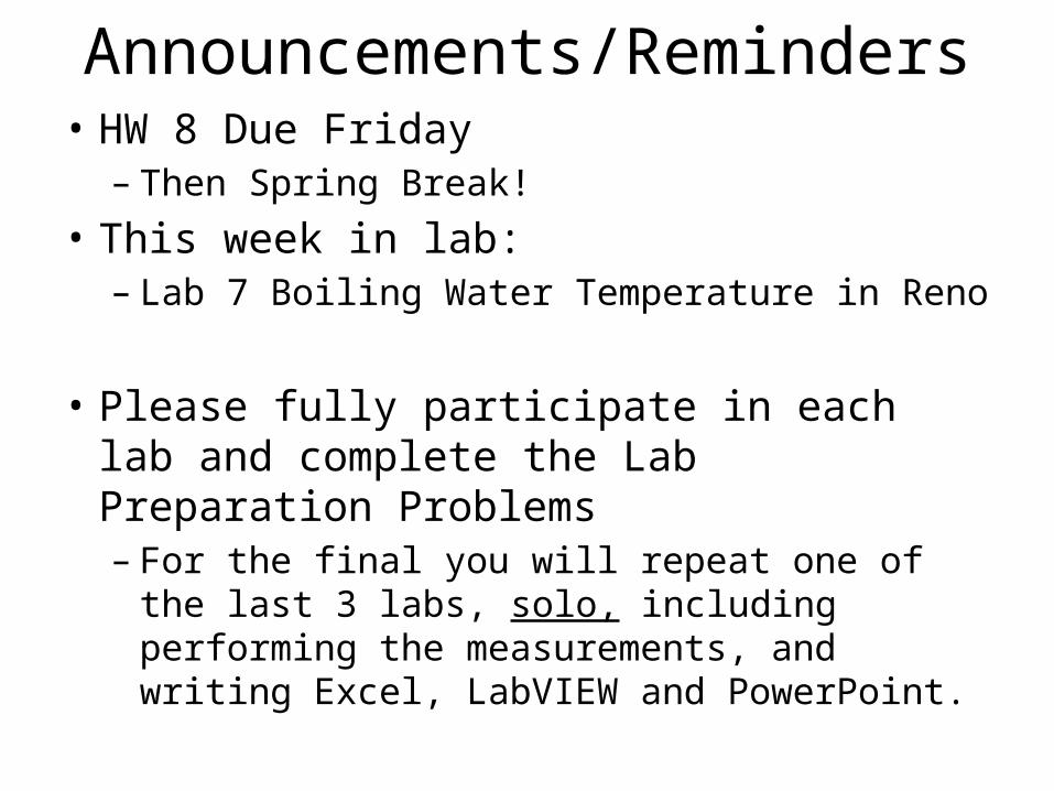
Announcements/Reminders• HW 8 Due Friday

– Then Spring Break!• This week in lab:

– Lab 7 Boiling Water Temperature in Reno

• Please fully participate in each lab and complete the Lab Preparation Problems– For the final you will repeat one of the last 3 labs,

solo, including performing the measurements, and writing Excel, LabVIEW and PowerPoint.

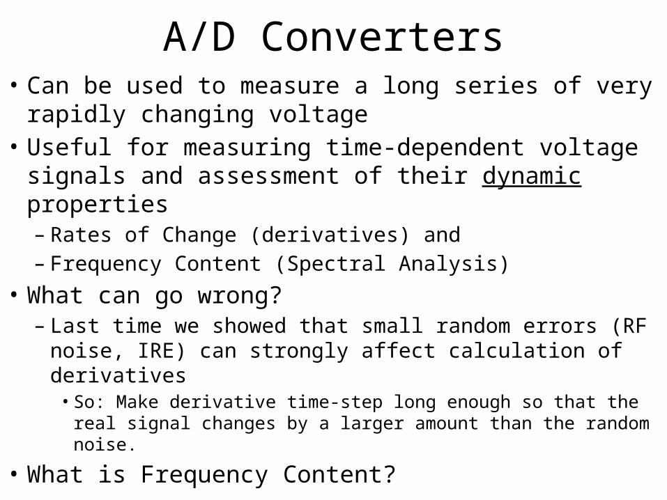
A/D Converters• Can be used to measure a long series of very rapidly

changing voltage • Useful for measuring time-dependent voltage signals

and assessment of their dynamic properties – Rates of Change (derivatives) and – Frequency Content (Spectral Analysis)

• What can go wrong?– Last time we showed that small random errors (RF noise,

IRE) can strongly affect calculation of derivatives• So: Make derivative time-step long enough so that the real

signal changes by a larger amount than the random noise.

• What is Frequency Content?

Spectral Analysis• Evaluates energy content associated with different

frequency components within a signal• Use to evaluate

– Tonal Content (music)• You hear notes, not time-varying pressure

– Dominant or natural frequencies • car vibration, beam or bell ringing

– System response (Vibration Analysis)• Resonance

• Spectral analysis transforms a signal from the time-domain V(t) to the frequency-domain, VRMS(f)– What does this mean?

Fourier Transform

• Any function V(t), over interval 0 < t < T1, may be decomposed into an infinite sum of sine and cosine waves– , – Only modes with an integer number of oscillations over the total sampling time T1 are

used.– Discrete (not continuous) frequencies: , n = 0, 1, 2, … ∞ (integers)– The coefficient’s an and bn quantify the relative importance (energy content) and phase of

each mode (wave). – The root-mean-square (RMS) coefficient for each mode frequency quantifies its total

energy content (both sine and cosine waves)

0 t T1

V

n = 0 n = 1 n = 2

sine

cosine

Examples (ME 322 Labs)

• Real signal may have a narrow or wide spectrum of energetic modes

Function Generator100 Hz sine wave

Unsteady air SpeedDownstream froma Cylinder in Cross

Flow

Time Domain Frequency Domain

-0.5

-0.4

-0.3

-0.2

-0.1

0

0.1

0.2

0.3

0.4

0.5

0 2 4 6 8 10

Time t [sec]

Dim

ensi

nole

ss A

ccel

erat

ion,

g t1 = 1.14 sec, a1 = 0.314 g

t2 = 5.88 sec, a2 = 0.152 g

0

0.02

0.04

0.06

0.08

0.1

0.12

0.14

0 10 20 30 40 50 60f [Hz]

a rm

s [g'

s]Damped VibratingCantilever Beam

What is the lowest Frequency mode that can be observed during measurement time T1

• Example– If we measure outdoor temperature for one hour, can we

observe variations that require a day to repeat?• The lowest (finite) observable frequency is f1 = 1/T1 • The only other frequencies that can be detected are

– (T1=nTn)

• What is the frequency resolution?– Smallest change in frequency that can be detected

• Increasing the total sampling time T1 reduces the lowest detectable frequency and improves frequency resolution,

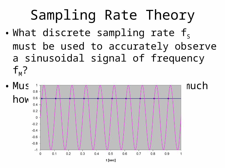
Sampling Rate Theory• What discrete sampling rate fS must be used to

accurately observe a sinusoidal signal of frequency fM?

• Must be greater than fM, but much how larger?

Lab 8 Aliasing Spreadsheet Example

• http://wolfweb.unr.edu/homepage/greiner/teaching/MECH322Instrumentation/Labs/Lab%2008%20Unsteady%20Voltage/Lab8Index.htm

• Measured sine wave, fm = 10 Hz– V(t) = (1volt)sin[2p(10Hz)(t+tshift)]

• Total sampling time, T1 = 1 sec• How many peaks to you expect to observe in one

second?• How large does the sampling rate fS need to be to

capture this many peaks?

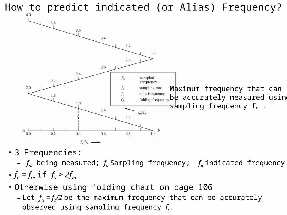
How to predict indicated (or Alias) Frequency?

• 3 Frequencies:– fm being measured; fs Sampling frequency; fa indicated frequency

• fa = fm if fs > 2fm • Otherwise using folding chart on page 106

– Let fN = fs/2 be the maximum frequency that can be accurately observed using sampling frequency fs.

Maximum frequency that canbe accurately measured usingsampling frequency fS .

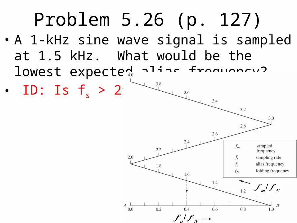
Problem 5.26 (p. 127)• A 1-kHz sine wave signal is sampled at 1.5 kHz.

What would be the lowest expected alias frequency?• ID: Is fs > 2fm ?

𝒇 𝒂 / 𝒇 𝑵

𝒇 𝒎/ 𝒇 𝑵

A more practical example

• Using a sampling frequency of 48,000 Hz, a peak in the spectral plot is observed at 18,000 Hz.

• What are the lowest 4 values of fm that can cause this?

• ID: what is known? fs and fa

18,000

Upper and Lower Frequency Limits

• If a signal is sampled at a rate of fS for a total time of T1 what are the highest and lowest frequencies that can be accurately detected?– (f1 = 1/T1) < f < (fN = fS/2)

• To reduce lowest frequency (and increase frequency resolution), increase total sampling time T1

• To observe higher frequencies, increase the sampling rate fS.

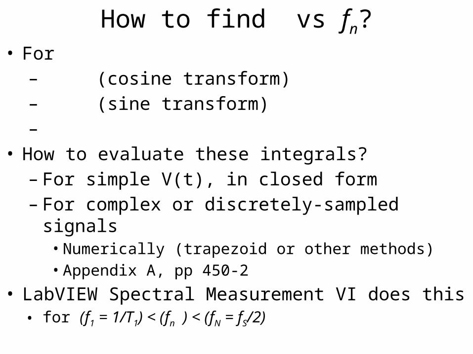
How to find vs fn?• For

– (cosine transform)– (sine transform)–

• How to evaluate these integrals? – For simple V(t), in closed form– For complex or discretely-sampled signals

• Numerically (trapezoid or other methods) • Appendix A, pp 450-2

• LabVIEW Spectral Measurement VI does this • for (f1 = 1/T1) < (fn ) < (fN = fS/2)

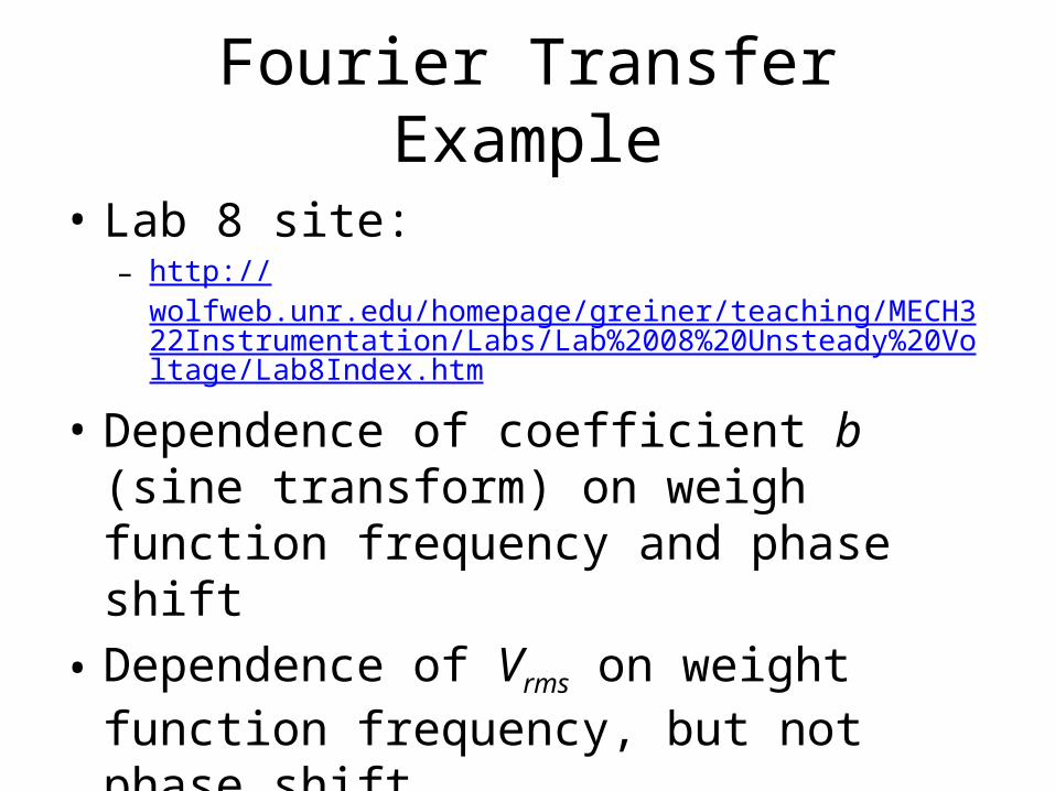
Fourier Transfer Example

• Lab 8 site:– http://

wolfweb.unr.edu/homepage/greiner/teaching/MECH322Instrumentation/Labs/Lab%2008%20Unsteady%20Voltage/Lab8Index.htm

• Dependence of coefficient b (sine transform) on weigh function frequency and phase shift

• Dependence of Vrms on weight function frequency, but not phase shift.

Lab 8: Time Varying Voltage Signals

• Produce sine and triangle waves with fm = 100 Hz, VPP = ±1-4 V– Sample both at fS = 48,000 Hz and numerically differentiate with two different differentiation time

steps• Evaluate Spectral Content of sine wave at four different sampling frequencies fS = 5000,

300, 150 and 70 Hz (note: some < 2 fm )• Sample singles between 10,000 Hz < fM < 100,000 Hz using fS = 48,000 Hz (fa compare to

folding chart)

Function Generator

Digital Scope

NI myDAQ

fM = 100 HzVPP = ±1 to ± 4 V Sine waveTriangle wave

fS = 100 or 48,000 HzTotal Sampling time T1 = 0.04 sec4 cycles 192,000 samples

Estimate Maximum Slope

• Sine wave • Triangle Wave

P P

VPP VPP

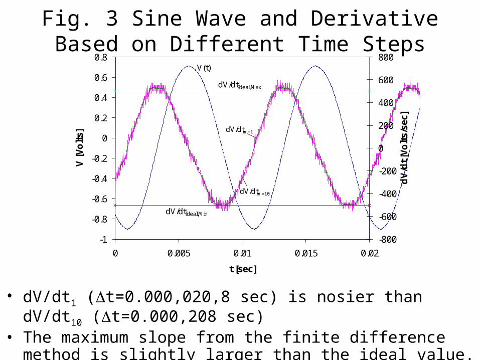
Fig. 3 Sine Wave and Derivative Based on Different Time Steps

• dV/dt1 (Dt=0.000,020,8 sec) is nosier than dV/dt10 (Dt=0.000,208 sec)• The maximum slope from the finite difference method is slightly

larger than the ideal value. This may be because the actual wave was not a pure sinusoidal.

-800

-600

-400

-200

0

200

400

600

800

-1

-0.8

-0.6

-0.4

-0.2

0

0.2

0.4

0.6

0.8

0 0.005 0.01 0.015 0.02

dV/d

t [Vo

lts/s

ec]

V [V

olts

]

t [sec]

dV/dtIdeal,Min

dV/dtIdeal,Max

V(t)

dV/dtm=1

dV/dtm=10

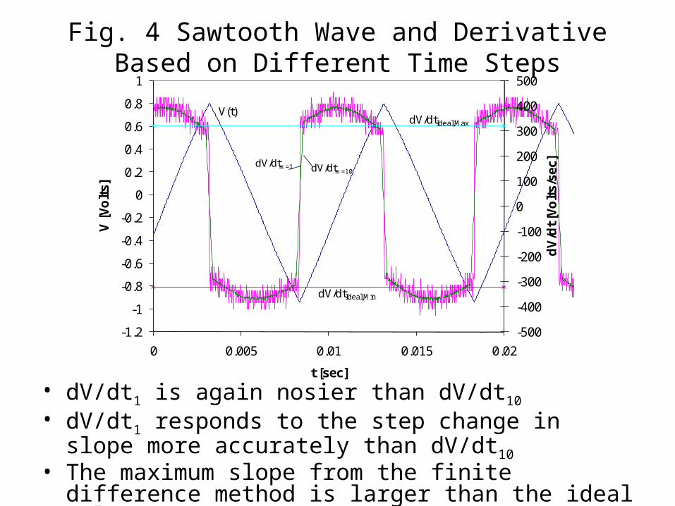
Fig. 4 Sawtooth Wave and Derivative Based on Different Time Steps

• dV/dt1 is again nosier than dV/dt10• dV/dt1 responds to the step change in slope more accurately

than dV/dt10• The maximum slope from the finite difference method is larger

than the ideal value.

-500

-400

-300

-200

-100

0

100

200

300

400

500

-1.2

-1

-0.8

-0.6

-0.4

-0.2

0

0.2

0.4

0.6

0.8

1

0 0.005 0.01 0.015 0.02

dV/d

t [Vo

lts/s

ec]

V [V

olts

]

t [sec]

dV/dtIdeal,Min

dV/dtIdeal,MaxV(t)

dV/dtm=1 dV/dtm=10

0

0.1

0.2

0.3

0.4

0.5

0.6

0 20 40 60 80 100 120 140 160 180 200

frecuency f [Hz]

V RM

S [V

olts

]

fs = 300 Hz fs = 5000 Hz

fs = 150 Hzfs = 70 Hz

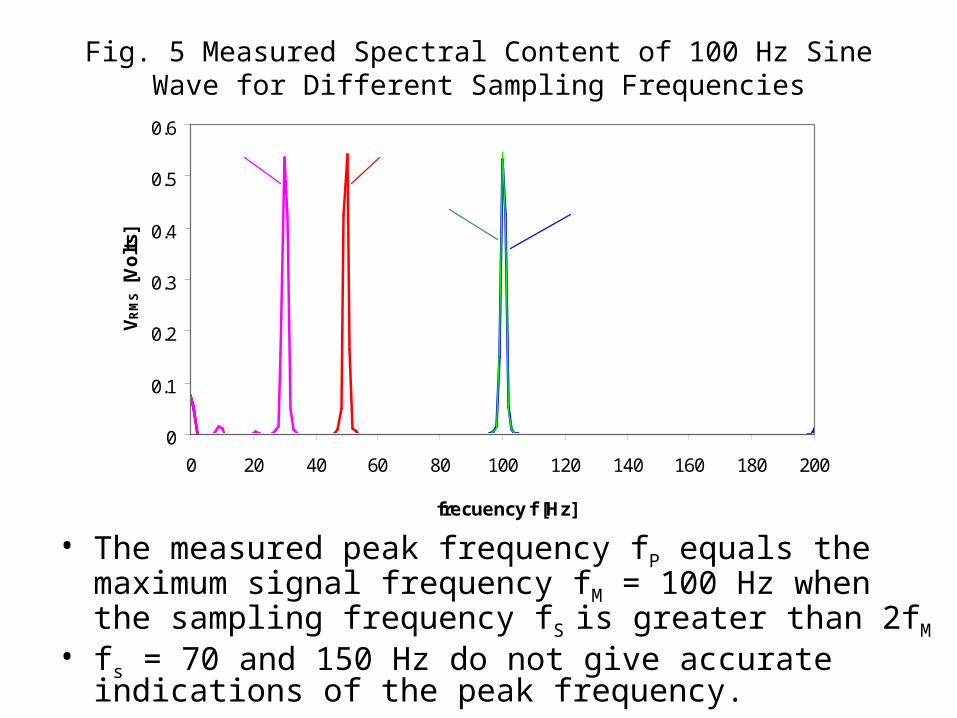
Fig. 5 Measured Spectral Content of 100 Hz Sine Wave for Different Sampling Frequencies

• The measured peak frequency fP equals the maximum signal frequency fM = 100 Hz when the sampling frequency fS is greater than 2fM

• fs = 70 and 150 Hz do not give accurate indications of the peak frequency.

Table 2 Peak Frequency versus Sampling Frequency

• For fS > 2fM = 200 Hz the measured peak is close to fM.

• For fS < 2fM the measured peak is close to the magnitude of fM–fS.

• The results are in agreement with sampling theory.

Sampling Frequency, fs [Hz] 5000 300 150 70Peak Spectral Frequency, fp [Hz] 100 100 50 30

Table 3 Signal and Indicated Frequency Data

• This table shows the dimensional and dimensionless signal frequency fm (measured by scope) and frequency indicated by spectral analysis, fa.

• For a sampling frequency of fS = 48,000 Hz, the folding frequency is fN = 24,000 Hz.

fm [Hz] fa [Hz] fm/fN fa/fN0 0 0.00 0.00

9910 9925 0.41 0.4119540 19575 0.81 0.8223120 23125 0.96 0.9630190 17800 1.26 0.7440510 7475 1.69 0.3147320 675 1.97 0.0350180 2175 2.09 0.0961200 13275 2.55 0.5571800 23850 2.99 0.9972400 23575 3.02 0.9879800 16125 3.33 0.6789500 6475 3.73 0.2795400 475 3.98 0.0299700 3725 4.15 0.16

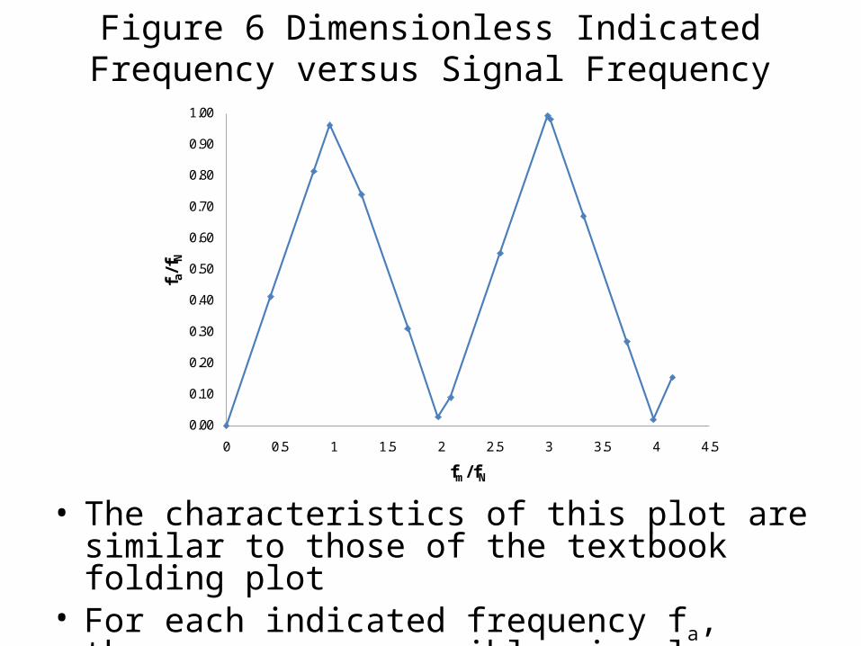
Figure 6 Dimensionless Indicated Frequency versus Signal Frequency

• The characteristics of this plot are similar to those of the textbook folding plot

• For each indicated frequency fa, there are many possible signal frequencies, fm.

0.00

0.10

0.20

0.30

0.40

0.50

0.60

0.70

0.80

0.90

1.00

0 0.5 1 1.5 2 2.5 3 3.5 4 4.5

f a/f

N

fm/fN

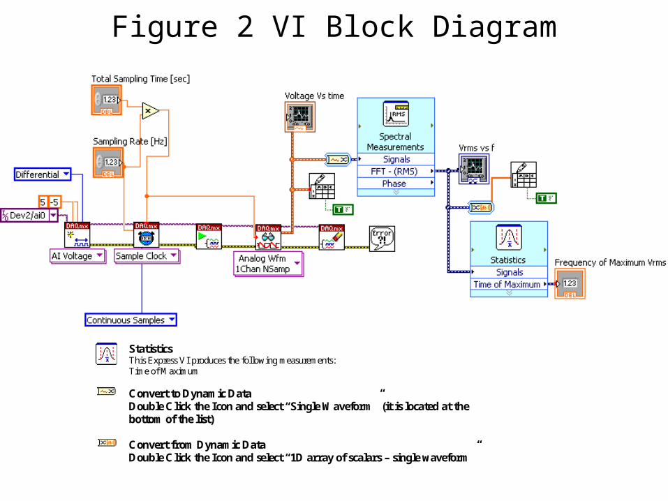
Figure 2 VI Block Diagram

Statistics This Express VI produces the following measurements: Time of Maximum

Convert to Dynamic Data Double Click the Icon and select “Single Waveform” (it is located at the bottom of the list)

Convert from Dynamic Data Double Click the Icon and select “1D array of scalars – single waveform”

Figure 1 VI Front Panel

Lab 8 Sample Data

• http://wolfweb.unr.edu/homepage/greiner/teaching/MECH322Instrumentation/Labs/Lab%2008%20Unsteady%20Voltage/Lab8Index.htm

• Calculate Derivatives• Plot using secondary axes• Frequency Domain Plot

– Lowest finite frequency f1 = 1/T1

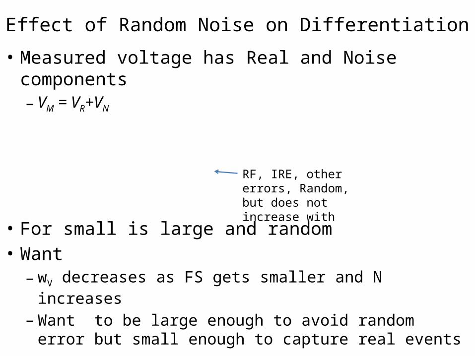
Effect of Random Noise on Differentiation• Measured voltage has Real and Noise components

– VM = VR+VN

• For small is large and random• Want

– wV decreases as FS gets smaller and N increases– Want to be large enough to avoid random error but small

enough to capture real events

RF, IRE, other errors, Random, but does not increase with

Time Dependent DataHow to find 1st order numerical differentiation (center difference)

= differentiation time

sampling time m = 1, 2, 3, …

i T = (∆ts)i V

0 0

1 ∆ts

2 2∆ts