1 ME-6950 Thermoelectric-I Summer-II 2015 Final Project Report Impact of Thomson Effect and Contact Resistance on a Thermoelectric Cooler Names: Pooja Iyer Mani-835408571 Shripad Dhoopagunta-166754583 Rajeev Chippa-750223327 Faculty: Dr. HoSung Lee Date of Submission: August 19 th , 2015
Transcript
1
ME-6950 Thermoelectric-I
Summer-II 2015
Final Project Report
Impact of Thomson Effect and Contact Resistance on a
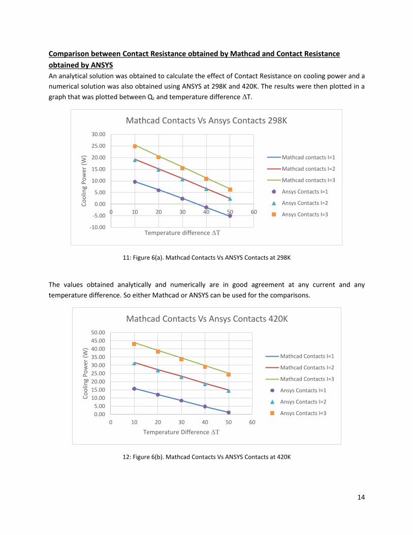
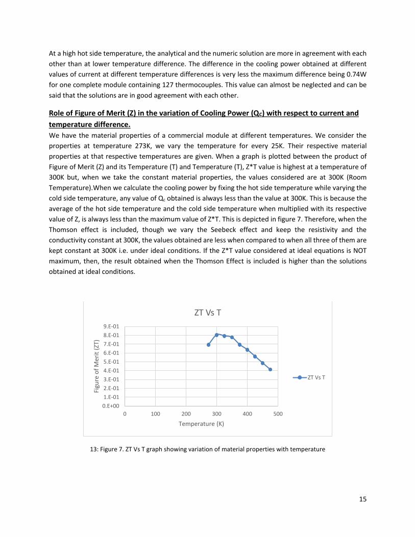
1). ANSYS Thermoelectric Cooler (TEC) Tutorial With Thomson effect and Contact Resistance
Preparing the ANSYS Workbench
1) Go Start Menu All Programs Simulation ANSYS 12.1 Workbench
2) In the toolbox menu on the left portion of the window, double click Thermal-Electric. A
project will now appear in the project schematic window of Workbench.
3) Right-click Thermal-Electric at the top of the Project Schematic pane and select Rename as
TEG Ex 3.1 Tutorial.
4) Save the project as Thermoelectric-Generator-Workbench.
Specifying the Materials and Properties
1) Double-click on Engineering Data to open the material data. You will see Structural Steel as the
default material in the Outline of Schematic A2: We are going to enter three materials (Copper
Alloy, p-type semiconductor, and n-type semiconductor) in the Engineering Data.
2) In the Data Source of Outline Filter, click on General Materials. In the Outline of General
Materials pane, right-click on Copper Alloy and select Add to Engineering Data or click on th
icon. A symbol will appear once the material has been added.
18
3) In the Outline Filter, click on Engineering Data, you will see that Copper Alloy in the Outline
Schematic A2 is newly added material to the Structural Steel.
4) Now we want to add two more materials (p-type and n-type semiconductors). Double-click on
Structural Steel and rename it as p-type. In the Toolbox pane, double-click Isotropic Thermal
Conductivity to include this property to the p-type.
5) In the Properties of Outline Row 5: p-type: The following values are entered as:
Isotropic Thermal Conductivity: 1.51 W m-1 K-1
Isotropic Resistivity: 0.00101 Ω cm
Isotropic Seebeck Coefficient: 202.17e-6 V K-1
For Thomson Effect Seebeck Coefficient varies with respect to Temperature. All these values can
be given in the tabular form in the Table of Properties Window. Continue the same with n-type.
19
6) Create n-type by duplicating the p-type. Right-click on p-type in the Outline of Schematic A2
and select Duplicate. A duplicate of the p-type material will appear below named p-type 2.
Rename this material to n-type. The value of the Isotropic Seebeck Coefficient is now changed
to the negative as–202.17e-6.
In the Properties of Outline Row 5: n-type: make sure the final values to be as:
Isotropic Thermal Conductivity: 1.51 W m-1 K-1
Isotropic Resistivity: 0.00101 Ω cm
Isotropic Seebeck Coefficient: –202.17e-6 V K-1
Input all the temperature dependent Seebeck Values for n-type. This is explained in the 5th
point.
7) Similarly add the third material Ceramic.
Isotropic Thermal Conductivity: 180 W m-1 K-1
Isotropic Resistivity: 10e14 Ω cm
8) Click on the icon in the menu bar to return to the Project.
9) Save the project.
20
Creating the Geometry
We are creating the following model, all the dimensions are mentioned here.
Dimensions are to the left hand side of the fig. The model is extruded to 0.41mm in the perpendicular
direction.
Example for creating the model. (The dimensions Mentioned from this section are just for an
Example)
1) In the project A under the Project Schematic, double-click on Geometry to launch the Design
Modeler.
2) Select Millimeter as the desired length unit and click OK.
3) In the Tree Outline pane, right-click on the XY Plane and select Look at. Add a new sketch by
clicking on the icon in the menu bar.
4) Sketch1 will appear below the XY Plane. Click on the Sketch1 and select the Sketching tab at
the bottom of the Tree Outline pane.
21
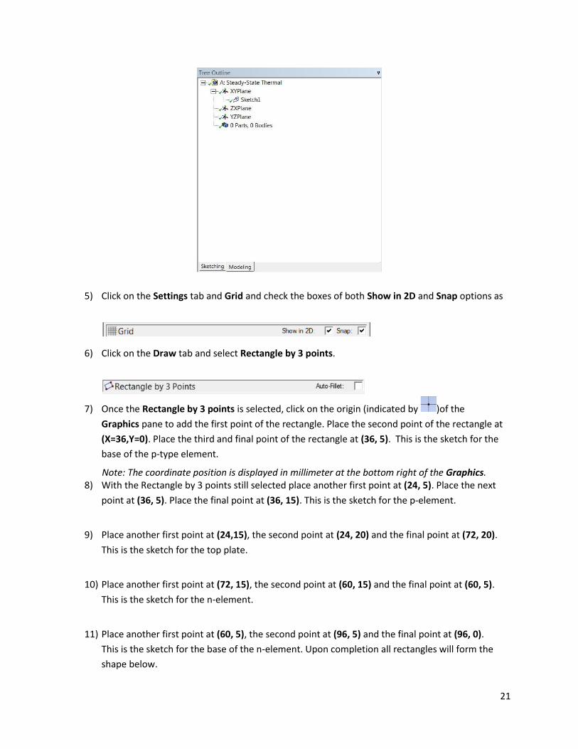
5) Click on the Settings tab and Grid and check the boxes of both Show in 2D and Snap options as
6) Click on the Draw tab and select Rectangle by 3 points.
7) Once the Rectangle by 3 points is selected, click on the origin (indicated by )of the
Graphics pane to add the first point of the rectangle. Place the second point of the rectangle at
(X=36,Y=0). Place the third and final point of the rectangle at (36, 5). This is the sketch for the
base of the p-type element.
Note: The coordinate position is displayed in millimeter at the bottom right of the Graphics. 8) With the Rectangle by 3 points still selected place another first point at (24, 5). Place the next
point at (36, 5). Place the final point at (36, 15). This is the sketch for the p-element.
9) Place another first point at (24,15), the second point at (24, 20) and the final point at (72, 20).
This is the sketch for the top plate.
10) Place another first point at (72, 15), the second point at (60, 15) and the final point at (60, 5).
This is the sketch for the n-element.
11) Place another first point at (60, 5), the second point at (96, 5) and the final point at (96, 0).
This is the sketch for the base of the n-element. Upon completion all rectangles will form the
shape below.
22
12) In the Tree Outline, click on the Modeling tab and select Sketch1 and extrude it by clicking the
icon in the menu bar or by going to Create Extrude on the menu bar.
13) Extrude1 will appear in the Tree Outline. Click on it. In the Details View pane, change the
Operation from Add Material to Add Frozen. Change the Depth to 10 mm.
Note: The ‘Add Frozen’ option keeps the various elements from merging. The ‘Add Material’ option will perform merging to one element.
14) To see an isometric view, click on the ball of the global coordiante axes.
15) Click on the icon in the menu bar to generate the extrusion or right-click on Extrude1 and
click Generate.
Note: The symbol will change to a symbol and, indicating that the command is successful.
16) In the Tree Outline, there will now be 5 Parts and 5 Bodies as a result of the extrusion.
23
17) Under the 7 Parts, 7 Bodies in the Tree Outline, select each body and rename it according to
the figure shown below. Rename each part by right-clicking on it in the Tree Outline and
selecting Rename. The currently selected part will become highlighted in the Graphics pane.
18) Ensure that each part is a Solid (by default) in the Details View pane under the Fluid/Solid
option. Select 7 bodies in the Tree Outline by clicking on them while holding down the Ctrl key.
Right-click and select Form a new part. Right-click and rename the part to TEC.
Finally the following bodies are created and have to be made into a single part.
19) Close the Design Modeler. Save the project from the Workbench.
p - base
top
n - base
p - leg
n - leg
24
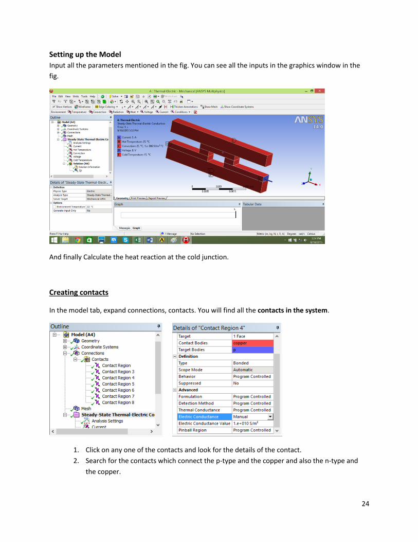
Setting up the Model
Input all the parameters mentioned in the fig. You can see all the inputs in the graphics window in the
fig.
And finally Calculate the heat reaction at the cold junction.
Creating contacts
In the model tab, expand connections, contacts. You will find all the contacts in the system.
1. Click on any one of the contacts and look for the details of the contact.
2. Search for the contacts which connect the p-type and the copper and also the n-type and
the copper.
25
3. You will find 4 such contacts. Select them individually and scroll down the details of the
contacts window.
4. Under Advanced tab set the Electrical conductance to manual and enter the value 1e+10
S/m^2.
Example for setting up the model.
This just an example the output of the program would be similar with different input and output
parameters.
In the Workbench, double-click on Model to launch the solver. This may take several seconds up to a
minute.
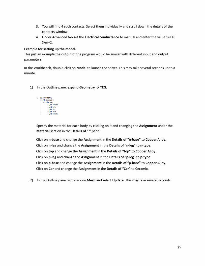
1) In the Outline pane, expand Geometry TEG.
Specify the material for each body by clicking on it and changing the Assignment under the
Material section in the Details of “ ” pane.
Click on n-base and change the Assignment in the Details of “n-base” to Copper Alloy.
Click on n-leg and change the Assignment in the Details of “n-leg” to n-type.
Click on top and change the Assignment in the Details of “top” to Copper Alloy.
Click on p-leg and change the Assignment in the Details of “p-leg” to p-type.
Click on p-base and change the Assignment in the Details of “p-base” to Copper Alloy.
Click on Cer and change the Assignment in the Details of “Cer” to Ceramic.
2) In the Outline pane right-click on Mesh and select Update. This may take several seconds.
26
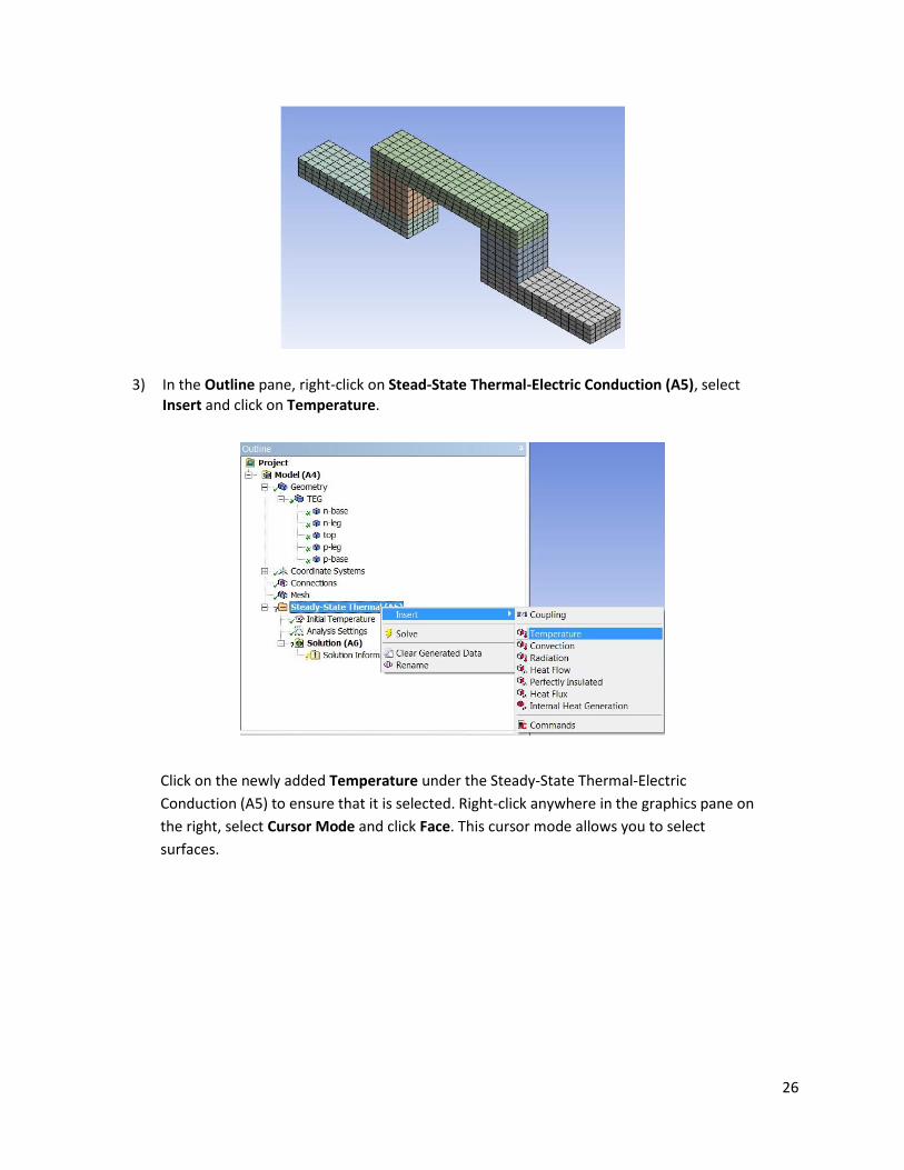
3) In the Outline pane, right-click on Stead-State Thermal-Electric Conduction (A5), select Insert and click on Temperature.
Click on the newly added Temperature under the Steady-State Thermal-Electric
Conduction (A5) to ensure that it is selected. Right-click anywhere in the graphics pane on
the right, select Cursor Mode and click Face. This cursor mode allows you to select
surfaces.
27
Click on the top surface of the top body to select it. Highlighted surfaces are indicated in
green. In the Details of “Temperature” pane, click Apply in the Geometry option. The
applied surface will change the color which confirms the application.
Change the Magnitude in the Details pane to 452 °C (ramped).
Right-click on Temperature in the Outline pane and rename it to Hot Junction. This is the hot
junction boundary condition.
28
4) In the Outline pane, right-click on Stead-State Thermal-Electric Conduction (A5), select Insert and click on Temperature again.
Note: Right-click anywhere in the Graphics pane and select Cursor Mode and click Rotate. Switch the cursor mode back to Face, click on the bottom surface of n-base and p-base while holding down Ctrl.
In the Details of “Temperature” pane, click Apply in the Geometry option. The applied
surface will change the color. Change the Magnitude in the Details pane to 22 °C
(ramped). Right-click on Temperature in the Outline pane and rename it to Cold
Junction. This is the cold junction boundary condition.
5) In the Outline pane, right-click on Stead-State Thermal-Electric Conduction (A5), select
Insert and click on Voltage .In the Graphics pane, change the view back to isometric by
clicking the small ball in the global coordinate axes. Select the outer face of the base of
the n-leg (parallel to the y-z plane).
In the Details of “Voltage” pane, click Apply in the Geometry option. The applied surface
will change the color. Ensure the Magnitude in the Details pane is 0 V (ramped). Right-
click on Voltage in the Outline pane and rename it to Low Potential. This is the lower
electric potential boundary condition. If current value has to be given, the low Voltage
(0V) is the same but the instead of high potential input current with desired value.
6) In the Outline pane, right-click on Stead-State Thermal-Electric Conduction (A5), select
Insert and click on Voltage again.
29
Note: Right-click anywhere in the Graphics pane and select Cursor Mode and click Rotate
and rotate the thermocouple until the other-side outer face of the base of the p-leg
(parallel to the y-z plane) can be seen. And select the outer face.
In the Details of “Voltage” pane, click Apply in the Geometry option. The applied surface
will change the color. Change the Magnitude in the Details pane is 0.08 V (ramped). Right-
click on Voltage in the Outline pane and rename it to High Potential. This is the higher
electric potential boundary condition.
7) In the Outline pane, right-click on Steady-State Thermal-Electric Conduction (A5), select
Insert and click on Convection. In the Graphics pane, select all faces excluding those
which have been assigned boundary conditions previously. Select multiple faces by
holding down the Ctrl key.
In the Details of “Convection” pane, click Apply in the Geometry option. The applied surface
will change the color. The Geometry option should read 21 Faces upon application. Change
the Magnitude in the Details pane is 1e-6 W/m2·°C (ramped) for negligible convection. Right-
click on Convection in the Outline pane and rename it to Insulation.
8) In the Outline pane, click on Steady-State Thermal-Electric Conduction (A5) to view the
boundary conditions selected as shown below.
30
9) In the Outline pane, right-click on Solution (A6), select Insert Thermal Temperature.
Make sure that All Bodies is default under Geometry in the Details of “Temperature”
pane. And leaves others as they are.
10) In the Outline pane, right-click on Solution (A6), select Electric Total Current Density.
Make sure that All Bodies is default under Geometry in the Details of “Total Current
Density” pane. And leaves others as they are. These render the desired results for display.
11) In the Outline pane, right-click on Solution (A6), select Probe Current Reaction. In the
Details of “Current reaction” pane, select Low Potential in the Boundary Condition
option. Right-click on Reaction Probe in the Outline pane and rename it to Current.
12) Repeat the insertion process for Probe Heat Reaction. In the Details of “Heat
Reaction” pane, select Hot Junction in the Boundary Condition option. Right-click on
Reaction Probe in the Outline pane and rename it to Hot Junction Heat Absorbed.
13) In the Outline pane, right-click Solution (A6) and click Solve or click on the
icon. The solver will take up to several minutes to complete.
14) Once the solver has completed its tasks, click on any of the solutions (Temperature, Total
Current Density, etc.) to display the results. For the Total Current Density, you can display
vectors (to indicate the direction of current flow) instead of contours by clicking on the
icon below the menu bar. Zoom in closer by scrolling up on the mouse wheel to
observe the direction of current. The results of the probes (Current and Hot Junction
Heat Absorbed), when selected, are displayed in Tabular Data pane at the bottom right
31
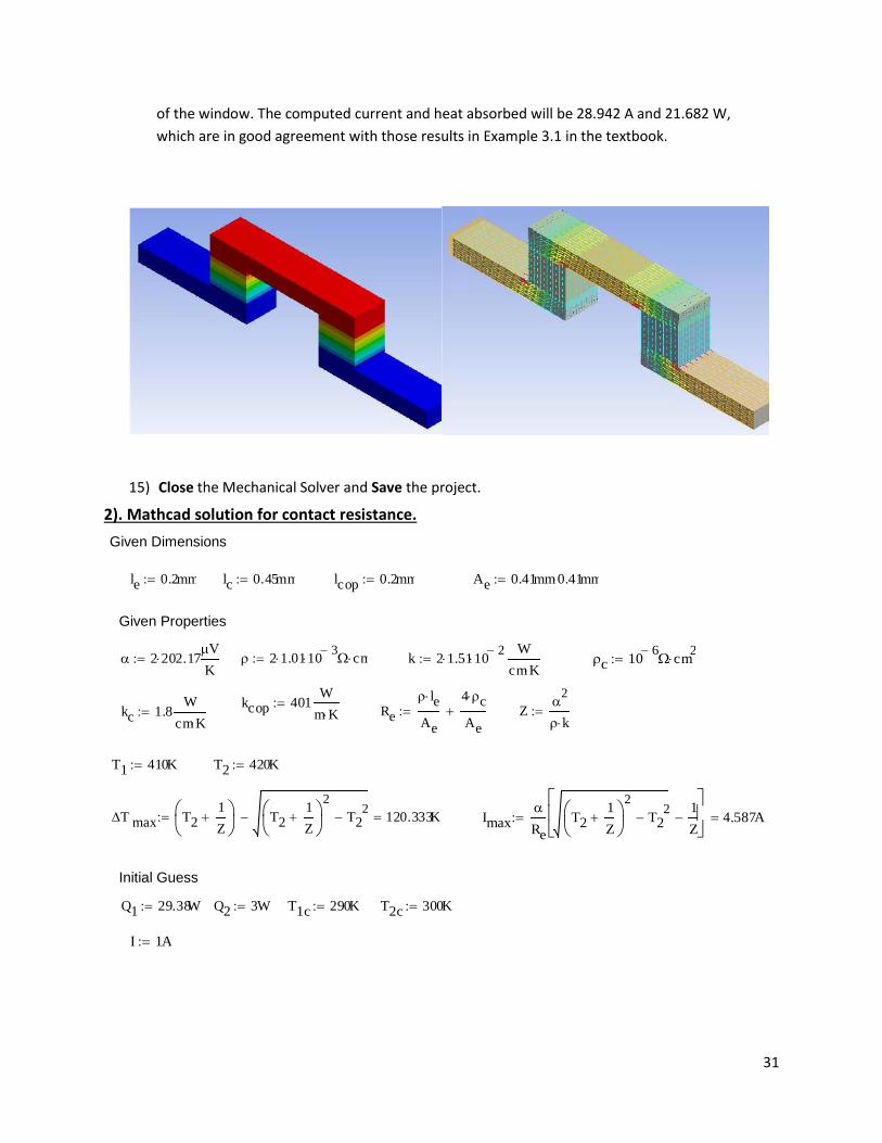
of the window. The computed current and heat absorbed will be 28.942 A and 21.682 W,
which are in good agreement with those results in Example 3.1 in the textbook.
15) Close the Mechanical Solver and Save the project.