47
1 ANALYSIS OF PIPE FLOW 9/21/2015 Pipes of different sizes and shapes are used in many industrial applications (Acknowledgement: Forchase Corporation Ltd, http://forchase.com)
| Date post: | 19-Feb-2016 |
| Category: |
Documents |
| Upload: | mohammad-taha |
| View: | 266 times |
| Download: | 1 times |

1
ANALYSIS OF PIPE FLOW
9/21/2015
Pipes of different sizes and shapes are used in many industrial applications
(Acknowledgement: Forchase Corporation Ltd, http://forchase.com)

2
To Malaysia
Water pipelines
Water pipelines between Malaysia and Singapore
(Acknowledgement: skyscrapercity.com)
Some examples of piping system in engineering applications
Pipelines in a petrochemical plant
(Acknowledgement: http://www.fullsupply.co.uk/)

3
Pipelines inside Honda Accord engine compartment
(Acknowledgement: Mark Gallagher)
Pipelines used in household appliances
(Acknowledgement:www.hotshowers.com) (Acknowledgement:www.bengreenplumbing.co.uk )

4
A satisfactory analysis of pipe flow depends on the accuracy involved inestimating the dissipation of energy incurred in maintaining the flow. Thisrequires the knowledge of boundary layer theory.
The following analysis relates to homogeneous fluid of constant viscosity anddensity. The results are also applicable to gases provided the densitychanges are small.
Types of Flow:
There are two types of flow in a pipe:
(a) Laminar Flow(b) Turbulent Flow

5
FLOW
This type of flow is characterized by motion of fluids in layers or laminas, parallel to the boundary surface.
(a) Laminar Flow:
Laminar flowFLOW
(b) Turbulent Flow:
Under certain conditions, a laminar flow can become unstable and become turbulent.
Laminar flow Turbulent flow
FLOW
FLOW
The turbulent flow is characterized by RANDOM, IRREGULAR and UNSTEADY movement of fluid particles, making it impossible to predict the motion of a fluid particle with respect to time and space.

6
Vdor
VdRed
The criteria which ascertain the type of flow is REYNOLD NUMBER (Re)
where =density of fluid, =dynamic viscosity, and =kinematic viscosity.
dV
Osborne Reynolds (a British Engineering Professor) was the first to show that the Reynolds number is the criterion for determining whether the flow is LAMINAR or TURBULENT in a circular pipe.
Red < 2300 (LAMINAR FLOW)
Critical Reynolds number is very sensitive to the initial disturbances in the fluid at the entrance.
By “quieting” the flow, it is possible to extend Red >50,000
The upper limit of critical Reynolds number depends on
(a) initial disturbance of approach flow,(b) shape of pipe entrance and(c) roughness of pipe.

7
FLOW NEAR ENTRANCE OF PIPE
Laminar Boundary Layer Turbulent Boundary Layer
Transitional Boundary Layer
dFlow
FLOW NEAR ENTRANCE OF PIPE
Laminar Flow
Very low velocity
Laminar B/L
Turbulent Flow
Very high velocity
Laminar B/L
Turbulent B/L

8
ENTRANCE LENGTH
Entrance length is defined as the distance from the entrance of the pipe that the flow needs to travel before the flow is fully developed (i.e. the velocity profile does not change with distance).
de Re
Vd
d
L
A B C
Velocity ProfileFully DevelopedProfile
Laminar Boundary Layer
Entrance Length (Le)
Laminar Flow
d
Figure P5(a)
The entrance length (Le) is a function of Reynolds number , i.e.
A B C
Velocity ProfileFully DevelopedProfile
Laminar Boundary Layer
Entrance Length (Le)
Laminar Flow
d
de Re06.0
d
L (LAMINAR)
The accepted correlation is
LAMINAR FLOW:
The maximum laminar entrance length at Red,critical = 2300 is Le=138d, which is the longest development length possible.

9
TURBULENT FLOW:
Laminar Boundary Layer
Turbulent Boundary Layer
Entrance Length (Le)
Fully DevelopedProfile
(a) Turbulent Flow
A B C
In turbulent flow, the boundary layers grow faster, and Le is relatively short. Based on the approximation
61
de Re4.4
d
L (TURBULENT)
The entrance length at various Reynolds number can be calculated as shown in the table below
Red Le/d
4000 18
104 20
105 30
106 44
107 65
EXAMPLE:
SAE 10 oil at 20oC flows through a 3-cm diameter tube. Estimate the entrance length in cm if the volume flow rate is (a) 0.001 m3/s and (b) 0.03 m3/s. The density () and dynamic viscosity () of SAE 10 oil are 870 kg/m3 and 0.104 kg/m.s, respectively.
d
Q4VdRe
Solution:Before we can determine the entrance length, we need to determine whether the flow is laminar or turbulent.
V4
dQ
2Volume flow rate
2d
Q4
V=
(a) Q=0.001m3/s
355)03.0)(104.0(
001.0)870(4Re
Flow is laminar since Re<2300.
From equation P1,
(b) Q=0.03 m3/s
10650)03.0)(104.0(
03.0)870(4Re
Flow is turbulent since Re>2300.
From equation P2,
cm64)3)(355(06.0Re06.0L de
cm62)3()10650(4.4Re4.4L 61
61
de
10
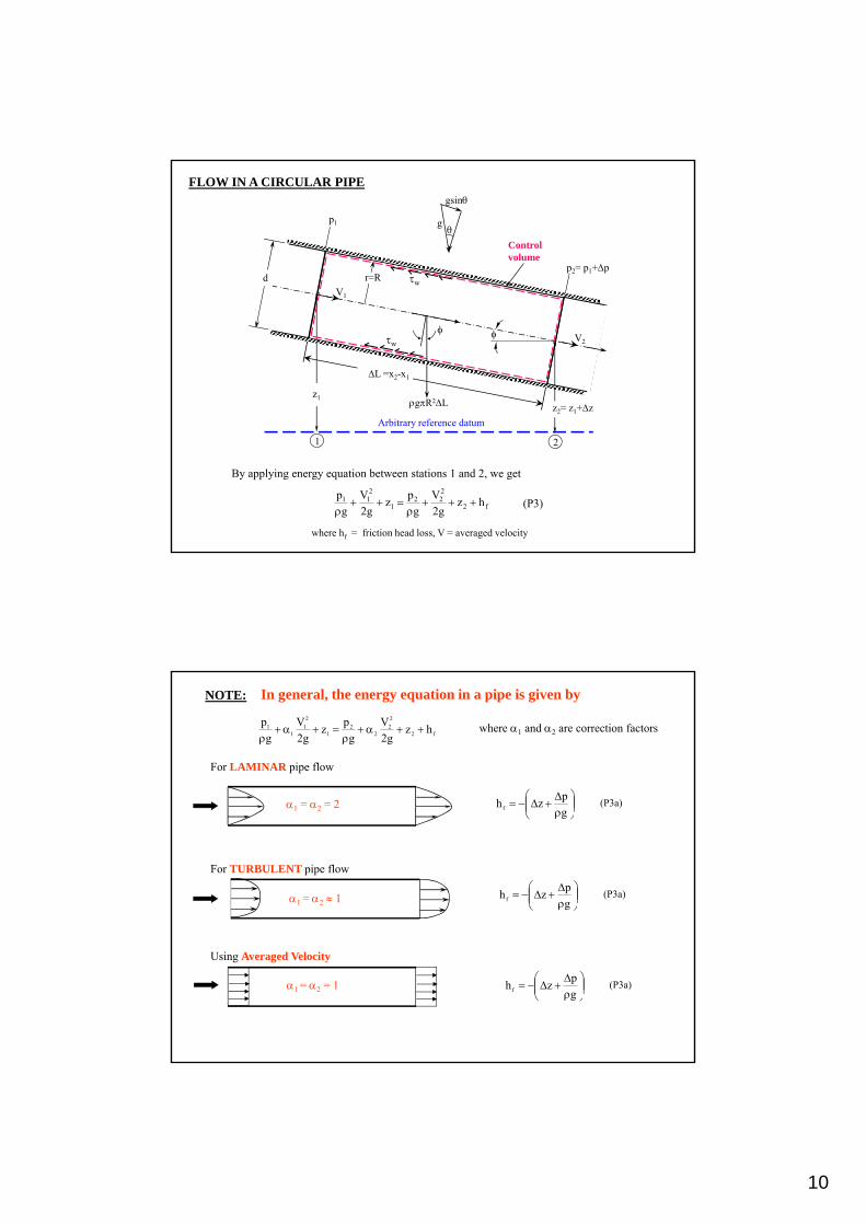
FLOW IN A CIRCULAR PIPE
By applying energy equation between stations 1 and 2, we get
f2
222
1
211 hz
g2
V
g
pz
g2
V
g
p
where hf = friction head loss, V = averaged velocity
(P3)
gsin
L =x2-x1
w
wV1
V2
z1
z2= z1+z
1
g
p1
p2= p1+pr=R
Arbitrary reference datum
2
gR2L
d
Control volume
In general, the energy equation in a pipe is given by
where 1 and 2 are correction factorsf2
2
22
21
2
11
1 hzg2
V
g
pz
g2
V
g
p
NOTE:
g
pzhf
(P3a)
g
pzhf
(P3a)
g
pzhf
(P3a)
For LAMINAR pipe flow
1 = 2 = 2
For TURBULENT pipe flow
1 = 2 1
Using Averaged Velocity
1 = 2 = 1

11
0VVmLR2sinLRgRpRp 12w22
22
1
0LR2sinLRgRp w22
zzzsinLBut 21
From the last slide, the energy loss (or head loss) is given by
-
g
pzhf (P3a)
Apply momentum equation to the control volume, we get
LR2zRgRp w22
)4P(gR
L2h
g
pzor w
f
Therefore, the above equation becomes
gsin
L =x2-x1
w
wV1
V2
z1z2= z1+z
1
gp1
p2= p1+p
r=R
Arbitrary reference datum 2
gR2L
)5P(V
8f
2w
Define the dimensionless parameter f (the Darcy Friction Factor)
By combining P4 and P5, the desired equation for pipe head loss
)4P(gR
L2h
g
pzor w
f
NOTE: Darcy-Weisbach Equation is valid for duct flows of any cross-section and both laminar and turbulent flow.
V = Average velocity
L
d
(Darcy-Weisbach Equation)
g2
V
d
Lfh
2
f (P6)

12
Rp
p +dp
dx
x
gr2dx
rdz
v1
v2
dx
-dz
Laminar Flow in a Circular Pipe
The laminar flow of an incompressible fluid under steady conditions may be completely analysed using Newton’s second law in the direction of motion..
2112222 vvcesin0)vv(mrdx2sindxrgr)dpp(rp
rdx2sindxrgrdp 22
rdx2dzrgrdp 22
gzpdx
d
2
r (P6a)
gzpdx
d
2
r
dr
du
gzpdx
d
2
r
dr
du
)7P(Cgzpdx
d
4
ru 1
2
Integrating gives
)8P(gzpdx
d
4
RC
2
1
Boundary condition: at r=R, u=0.
Note that velocity gradient, du/dr, is negative i.e. as r increases u decreases,
dr
du
The shear stress is related to the velocity gradient by
(P6b)
Substituting (P6b) into (P6a) gives gzpdx
d
2
r (P6a)
Substitute into equation (P7) gives
C1 is a constant that depends on the boundary condition.

13
After substituting (P8) into equation (P7), the velocity distribution is given by
which is a parabolic distribution. Equation (P9) iscalled the Hagen-Poiseuille Flow.
FLOW
uR
r
22 rRgzpdx
d
4
1u
(P9)
Note: Equation (P9) applies to Laminar Flow Only
gzpdx
d
4
ru
2
gzpdx
d
4
R 2
22 rRgzpdx
d
4
1u
)10P(gzpdx
d
4
Ru
2
max
Maximum velocity occurs at the centre of the pipe, i.e. r=0
FLOW
uRr umax
To find average volume flow rate (Q) [m3/s],
R
0
rdru.2Q
R
0
22 rdr2rRgzpdx
d
4
1Q
)11P(gzpdx
d
8
R 4
Therefore, dQ = u.2rdr
r
dr
Figure P8
R
Shaded area = (r+dr)2-(r)2
2rdr (since dr is small)
We consider flow through a GREEN circular ring
22 rRgzpdx
d
4
1u
From laminar velocity profile (P9)

14
Comparing equation (P10) and (P11), it can be seen that
gzpdx
d
4
RR
2
1gzp
dx
d
8
RQ
22
4
umax
max2uR
2
1Q
)a11P(2
u
A
Q)velocityaverage(VBut max
Similarly, shear stress (), friction factor (f) and head loss (h) can be determined as follows
)b11P(R
u2gzp
dx
d
4
R
R
2gzp
dx
d
2
R
dr
du max2
Rrw
)12P(Re
64
V
8f
d2
warminla
)13P(gd
LQ128
g2
V
d
Lfh 4
2
arminlaarminla,f
22 rRgzpdx
d
4
1u
(P9)
Pressure Drop for a Laminar Flow in a Horizontal Pipe
gzpdx
d
8
RQ
4
)14P(dx
dzg
dx
dp
8
R4
From equation (P11),
Assuming that the length of the pipe is L; p=change in pressure over the length of the pipe, and z=change of elevation.
L
zg
L
p
8
RQ
4
z1z2
Lp1
p1+p
Datum
Equation (P14) becomes
)15P(R
LQ8p
4
If the pipe is horizontal z=0, therefore
for laminar flow only
Introducing R=d/2
)16P(d
LQ128p 4

15
TURBULENT FLOW IN A CIRCULAR PIPE
Turbulent Flow in a Circular Pipe
d V
Laminar(PARABOLIC)
Turbulent
In turbulent flow, a major part of the mechanical energy in the flow goes into forming and maintaining randomly eddying motion.
Eddying motion dissipates their kinetic energy into heat.
At a given Reynolds number, the drag of the turbulent flow is higher than the drag of a laminar flow.
Turbulent flow is affected by surface roughness, so that increasing roughness increases the drag.

16
TURBULENT FLOW THROUGH SMOOTH PIPE
For turbulent flows, there are no exact solutions available for the velocity profile and the friction factor variation with Reynolds number, and we must always rely on experimental data.
VELOCITY Profile
For turbulent flow near a wall, the boundary layer can be divided into three regions. They are the WALL LAYER, the OVERLAP LAYER and the OUTER LAYER.
Outer layer
Overlap layer
Wall layer (or viscous sub-layer)Figure P10
Wall
Rr
uy
Umax
Turbulent Flow
Wall
uy
Outer layer
Umax
Turbulent Flow
Overlap layer
Wall layer (or viscous sublayer)
Rr
)17P(*yu
offunction*u
u
wwhere y = (R-r), =kinematic viscosity of fluid, and u*= which is called the friction velocity.
FOR THE WALL LAYER: Viscous shear (laminar) dominates. Using dimensional analysis, Prandtl deduced in 1930 that
Experiment indicates that
)17P(*yu
*u
u
*u)rR(
*u
u or
Equation (P17) is called the LAW OF THE WALL.

17
Wall
uy
Outer layer
Umax
Turbulent Flow
Overlap layer
Wall layer (or viscous sublayer)
Rr
FOR THE OUTER LAYER: Turbulent shear dominates. Using dimensional analysis,Von Karman deduced in 1933 that
orR
yfunction
*u
uUmax
)18P(
R
rRfunction
*u
uUmax
Umax-u is called the velocity defect, and equation (P18) is called VELOCITY DEFECT LAW
orB*yu
ln1
*u
u
)19P(B
*u)rR(ln
1
*u
u
FOR THE OVERLAP LAYER: Both viscous and turbulent shear dominate. C. B. Milliken in 1937 showed, using dimensional analysis, that
where and B are constant. Experimental data show that =0.4 and B=5.0. Equation (P19) is called the LOGARITHMIC OVERLAP LAYER
Wall
uy
Outer layer
Umax
Turbulent Flow
Overlap layer
Wall layer (or viscous sublayer)
Rr

18
orB*yu
ln1
*u
u
)19P(B
*u)rR(ln
1
*u
u
=0.4 B=5.0
10o 101 102 103 1040
10
20
30
u/u* Eqn (P17)
5 30
Viscous sublayer Buffer layer Overlap layer
Experimental dataOuter layer
*yu
)a19P(B*Ru
ln1
*u
Umax
(P19) minus (P19a) gives
A good approximation for the OUTER TURBULENT BOUNDARY OF THE PIPE can be obtained from (P19) by setting u=Umax when r=0 because maximum velocity occurs at the centre of the pipe, i.e.
)19P(B*u)rR(
ln1
*u
u
rR
Rln
1
*u
uUmax

19
(b) Relationship between mean velocity (V) and maximum velocity (umax)for a turbulent flow in a pipe
Rr
u
umax
B
*urRn
1
*u
ru
No exact solutions available for the velocity profile of a smooth turbulent flow, however experimental data follow a logarithmic relation.
)19Peqnfrom(B
*urRn
1
*u
ru
where =0.4 and B=5.0.
ru means that u is a function of r.NOTE:
)20P(
R
dr.r2.ruV
2
R
0
A
QV
The mean (or average velocity) V in the pipe is given by
)21P(rdr2B
*urRn
1*u
R
1V
R
02
B
*urRn
1*uru Substituting from the above into eqn (P20a),
we get
Mean (or average velocity) V
r
dr
Figure P8
R
Shaded area = (r+dr)2-(r)2
2rdr (since dr is small)
where Q= volume flow rate and A is the pipe cross-sectional area

20
b
ax
2
x
2
1bxan
b
ax
2
1xdxbxan
2
2
22
To solve the above integral (P21), we can refer to the Handbook of Mathematical Formulas and Integrals by Jeffrey Alan ( 2nd edition, Academic Press, pg 176). Relevance formulation is reproduced here
3B2
*Run
2*u
2
1V
Using the above formulation, equation P21 can be simplified to give
Substituting =0.40 and B=5.0 into the above equation, we obtain
)22P(25.1*Ru
n5.2*u
V
Since the maximum velocity (umax) occurs at the location where r=0. (P20) becomes
)23P(0.5*Ru
n5.2*u
umax
25.10.5*u
Vumax
)24P(V
*u75.31
V
umax
f
8
*u
V
f33.118
f75.31
V
umax
)25P(f33.11
1
u
V
max
Subtract (P22) from (P23), we get
Substitute the above into (P24) gives
w*u 2w
V
8f
But , and simple manipulation givesand
)22P(25.1*Ru
n5.2*u
V
)23P(0.5*Ru
n5.2*u
umax

21
(c) Friction Factor
)26P(8.0fRelog0.2f
1d
The relationship between friction factor and Reynolds number for a smooth turbulent pipe flow is given semi-empirical as
Which is known as PRANDTL’S UNIVERSAL LAW OF FRICTION for smooth pipe (for derivation, see Shames)
Some numerical values of equation P26 is listed below
Red 4000 104 105 106 107 108
f 0.0399 0.0309 0.0180 0.0116 0.0081 0.0059
Note that f drops by only a factor of 5 over a 10,000-fold increase in Reynolds number.
Graphically, equation (P26) can be plotted together with equation (P12) for smooth pipe laminar flow as shown in the graph below
)12P(f arminlaRe
64
d
103 104 105 106 107 108
0.01
0.02
0.03
0.04
0.05
0.06
0.070.080.090.10
f
Reynolds number (Red)
Smooth pipe: Laminar flow (eqn P12)
dRe
64f
Smooth pipe: Turbulent flow (eqn 26)
8.0fRelog0.2f
1d
)27P(10Re4000Re316.0f 5d
41
d
There are many alternatives of finding f, one of which is by Blasius is
Equation P26 is quite cumbersome to solve if Red is known and f is required.

22
Pressure Drop for a Turbulent Flow in a Smooth Horizontal Pipe
Frictional loss in the pipe (laminar or turbulent) is given by
g2
V
d
Lfz
g
ph
2
f
Eqn (3a) Eqn (6)
g2
V
d
Lf
g
ph
2
f
If the pipe is horizontal z=0
Substituting f from equation (P27) into the above equation we get
g2
V
d
L
Vd316.0
g2
V
d
Lf
g
ph
24
12
f
Eqn (27)
4
7
4
54
1
4
3
VdL158.0p
75.125.141
43
VdL158.0p
Vd4
1QgIntroducin 2
)27P(Re316.0f 41
d
flowturbulentforQdL241.0p 75.175.441
43
(P28)
Compare with pressure drop in laminar flow for a horizontal pipe
Note:
(a) For a given Q, the pressure drop in turbulent flow decrease more quickly than in laminar flow.
(b) The quickest way to reduce the required pumping pressure is to increase the diameter of the pipe. Doubling the pipe reduces p by a factor of about 27.
ord
LQ128p
4
)29P(QLd128
p4
For LAMINAR flow
(P28)QdL241.0p 75.175.44
1
4
3 For TURBULENT flow

23
Pipe 1
Pipe 2
Q
Q
d
2d
L
L
Pressure Drop (P1)
27
PP 1
2
TURBULENT FLOW
Better to transport water from Malaysia to Singapore using a big pipe, but the cost of the pipe will go up!
TURBULENT FLOW through A ROUGH PIPE

24
FLOW THROUGH ROUGH PIPES
•Most of the pipes used in engineering applications such as cement pipes, cast iron pipes etc cannot be regarded as hydraulically smooth especially at high Reynolds numbers.
•In fact, they are actually behaving as hydraulically rough.
•The resistance to fluid flow offered by rough boundaries is larger that for smooth boundaries on account of formation of eddies behind rough protrusions.
•For LAMINAR FLOW, all rough pipes irrespective of their roughness size and pattern offer the same resistance as that offered by a smooth pipe under similar conditions of flow.
•In fact, there is no surface which may be regarded as perfectly smooth. The term “smooth” and “rough” are relative.
•In turbulent flow, there is a thin layer very close to the boundary in which the flow exhibits characteristics of laminar flow. This layer is call “laminar sublayer”
Limit of laminarsublayer
Turbulent flow
Turbulent boundary layer
Limit of laminar sublayer Roughness elements completely
submerged in the laminar sublayer
Figure P13
This occurs when the roughness elements are submerged in the laminar sublayer, and therefore have no effects on friction
)30P(5*u
Criteria for Hydraulically Smooth Walls:
w*urecall that and = kinematic viscosity of fluid
(a)Hydraulically Smooth Walls

25
Limit of laminar sublayerRoughness elements protrude into the main flow
Figure P14
(b) Hydraulically Rough Walls
This occurs when the roughness elements protrude into the main flow causing it to break up into vortices or eddies.
)31P(70*u
Criteria for Hydraulically Rough Walls:
Limit of laminar sublayer
Some roughness elements are submerged and some are protruded into the main flow
Figure P15
(c) Transitional Roughness:
The regime lies between hydraulically smooth wall and hydraulically rough walls.
)32P(70*u
5
Criteria for Transitional Roughness:

26
EXAMPLE:
Water at 20 oC flows in a 10 cm diameter pipe at an average velocity of 1.6 m/s. If the roughnesselements are 0.046 mm high and the friction factor is f = 0.0204, would the wall be considered roughor smooth? Assume the kinematic viscosity of water () 10-6 m2/s.
5*u
If
70*u
If
Solution:
then the wall is hydraulically smooth.
then the wall would be rough.
To find if the wall is smooth, we need to make use of the flow criteria:
Pa53.60204.06.110008
1fV
8
1 22
s/m0808.01000
53.6*u w
7.3
10
0808.010x046.0*u6
3
The friction velocity is
Therefore the wall is hydraulically smooth, even though it is physically rough.
Therefore, the viscous wall layer thickness is
Velocity Profile in a Rough Pipe

27
Limit of laminar sublayer
Roughness elements completely submerged in the laminar sublayer
(a) Velocity Profile in a Rough Pipe:
The velocity profiles in a rough pipe depend on whether the pipe is hydraulically smoothor completely rough or Transitional rough.
(a) hydraulically Smooth
For hydraulically smooth pipe, the roughness elements are submerged inside laminar boundary layer.
)33P(0.5*yu
ln4.0
1
*u
u
We may use the velocity profile for a smooth pipe, i.e.
Limit of laminar sublayer
Roughness elements protrude through laminar sublayer
Figure P16
(b) Completely Rough
The velocity profile for a completely rough pipe is
5.8y
ln4.0
1
*u
u
28
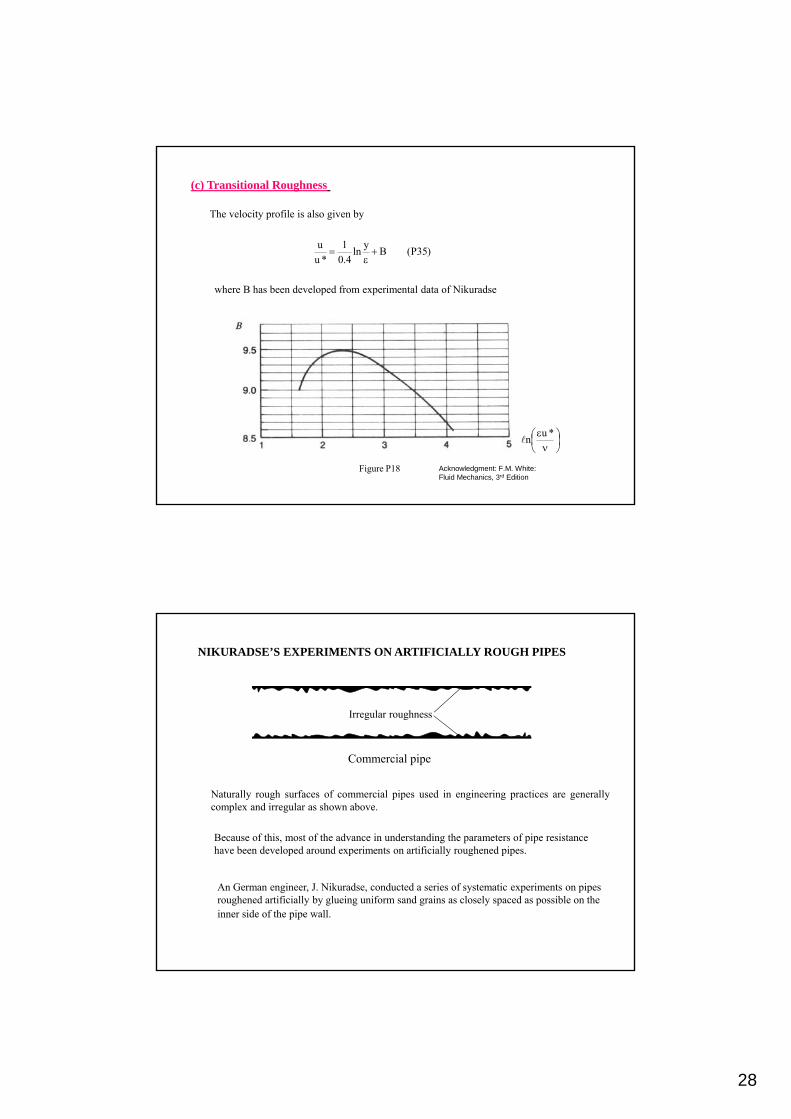
)35P(By
ln4.0
1
*u
u
*u
n
Figure P18 Acknowledgment: F.M. White: Fluid Mechanics, 3rd Edition
(c) Transitional Roughness
where B has been developed from experimental data of Nikuradse
The velocity profile is also given by
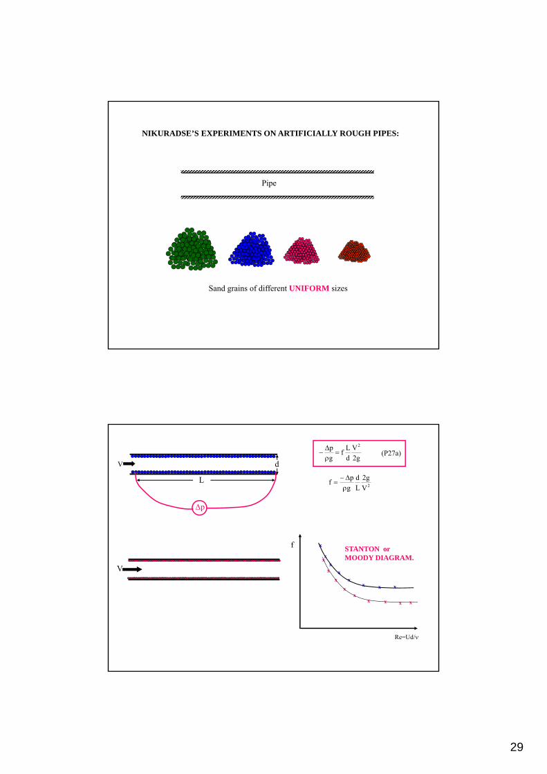
NIKURADSE’S EXPERIMENTS ON ARTIFICIALLY ROUGH PIPES
Irregular roughness
Commercial pipe
Naturally rough surfaces of commercial pipes used in engineering practices are generallycomplex and irregular as shown above.
Because of this, most of the advance in understanding the parameters of pipe resistancehave been developed around experiments on artificially roughened pipes.
An German engineer, J. Nikuradse, conducted a series of systematic experiments on pipes roughened artificially by glueing uniform sand grains as closely spaced as possible on the inner side of the pipe wall.
29
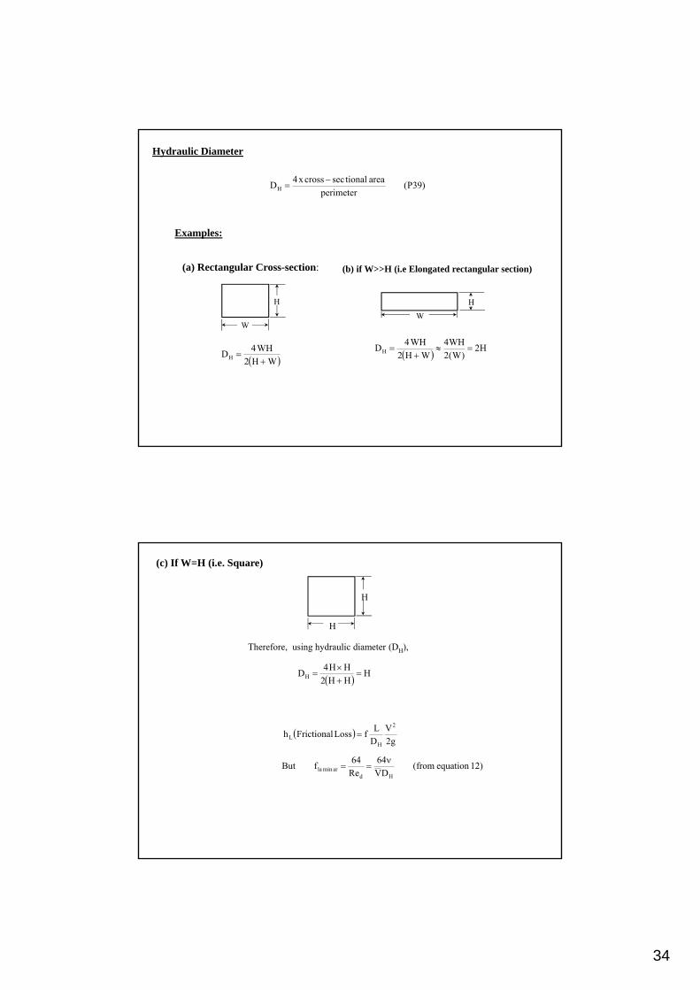
NIKURADSE’S EXPERIMENTS ON ARTIFICIALLY ROUGH PIPES:
Sand grains of different UNIFORM sizes
Pipe
f
Re=Ud/
L
d
2V
g2
L
d
g
pf
V
x
x
p
g2
V
d
Lf
g
p 2
(P27a)
xxx
x
x
x
x
x x
STANTON orMOODY DIAGRAM.
xx
x
x
x x
V

30
A
B
COMPLETELY TURBULENT REGIME
C
D
LAMINARFLOW
F
E
SMOOTH PIPES
8.0fRelog0.2f
1d
STANTON or MOODY DIAGRAM
STANTON or MOODY DIAGRAM
For all the curves on the right hand side of AB (red curve), the f versus Reynolds number relationship becomes horizontal indicating that friction factor is independent of the Reynolds number. This region is identified as a fully rough flow, and are described by
7.3
dlog0.2
f
1(P36) (see page 163 of your notes)
A
B
COMPLETELY TURBULENT REGIME
8.0fRelog0.2f
1d
Smooth pipe
(P26)

31
Between lines EF and AB, the friction factor is dependent on both Reynolds number as well as the relative roughness.
Colebrook in 1939 cleverly combined the smooth wall (equation P26) and fully rough flow (equation P36) relations into an interpolated formula.
A
B
COMPLETELY TURBULENT REGIME
E
F
7.3
dεlog0.2
f
1
(P36)
8.0fRelog0.2f
1d
Smooth pipe
(P26)
fRe
51.2
7.3
dεlog0.2
f
1
d
(P37)
But equation (P37) is difficult to use
(see page 163 of your notes)
An alternative formula given by Haaland is given by
11.1
d 7.3
d
Re
9.6log8.1
f
1
which varies less than 2% from equation
(P38)
fRe
51.2
7.3
dεlog0.2
f
1
d
(P37)
A
B
COMPLETELY TURBULENT REGIME
E
F
7.3
dεlog0.2
f
1
(P36)
8.0fRelog0.2f
1d
Smooth pipe
(P26)

32
0.0128
0.0185
0.0125
The Moody Diagram is accurate to 15% for design calculations over the fullrange shown in the figure. The shaded area in the Moody diagram indicates the rangewhere transition from laminar to turbulent flow occurs. There are no reliable frictionfactors in this range, 2000<Red<4000.

33
AVERAGE ROUGHNESS OF COMMERCIAL PIPES
Material (new) (mm)
Riveted steel 0.9-9.0
Concrete 0.3-3.0
Cast iron 0.26
Galvanised iron 0.15
Asphalted cast iron 0.12
Commercial steel or wrought iron 0.046
Drawn tubing 0.0015
Glass “Smooth”
From: F.M. White, Fluid Mechanics, 3rd Edition
Friction in Non-circular Pipes
Most of the pipes or conduits used in engineering applications are circular in cross-section.
On some occasions, we also use rectangular ducts and cross sections of other geometry.
We can modify many of the equations that we have derived earlier for circular cross-sections to noncircular sections by using the concept of HYDRAULIC DIAMETER.
Circular pipes
(Acknowledgement: Rigidtools.org)
Non-circular pipes
(Acknowledgement: itctubeco.com)
34
)39P(perimeter
areationalseccrossx4DH
Examples:
H2)W(2
WH4
WH2
WH4DH
W
H
(b) if W>>H (i.e Elongated rectangular section)
WH2
WH4DH
W
H
(a) Rectangular Cross-section:
Hydraulic Diameter
HHH2
HH4DH
g2
V
D
LfLossFrictionalh
2
HL
)12equationfrom(DV
64
Re
64fBut
Hdarminla
H
H
(c) If W=H (i.e. Square)
Therefore, using hydraulic diameter (DH),

35
HYDRAULIC DIAMETER APPROACH gives
A reasonable accurate result for turbulent flow.
But not so accurate for laminar flow.
WHY??
In laminar flow viscous action causes friction phenomenon to occur throughout the fluid.
In turbulent flow, most of the action occurs in the region close to the wall, i.e. it depends onthe wetted perimeter.
d V
Laminar(PARABOLIC)
Turbulent
Minor Losses in Pipes
36
Bends
Valve
Sudden enlargement
Sudden contraction
FittingsInlet
Outlet
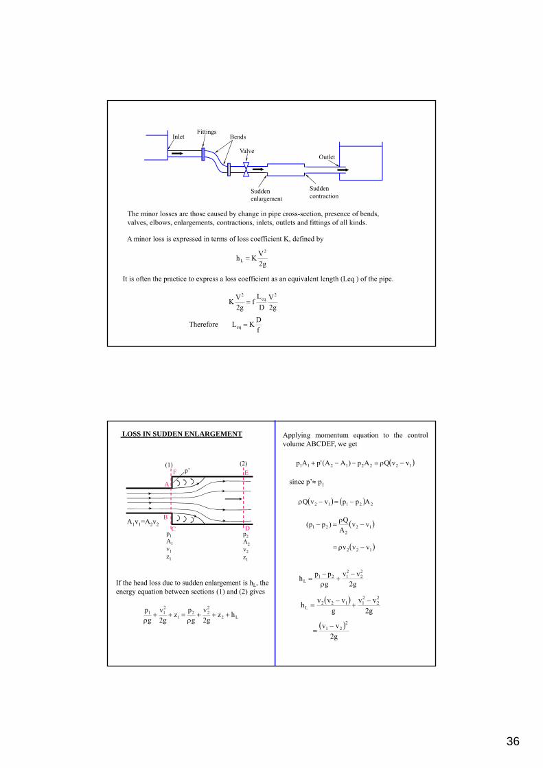
The minor losses are those caused by change in pipe cross-section, presence of bends, valves, elbows, enlargements, contractions, inlets, outlets and fittings of all kinds.
A minor loss is expressed in terms of loss coefficient K, defined by
g2
VKh
2
L
It is often the practice to express a loss coefficient as an equivalent length (Leq ) of the pipe.
g2
V
D
Lf
g2
VK
2eq
2
f
DKLTherefore eq
LOSS IN SUDDEN ENLARGEMENT
If the head loss due to sudden enlargement is hL, the energy equation between sections (1) and (2) gives
L2
222
1
211 hz
g2
v
g
pz
g2
v
g
p
Applying momentum equation to the controlvolume ABCDEF, we get
12221211 vvQAp)AA('pAp
22112 AppvvQ
122
21 vvA
Q)pp(
122 vvv
since p’ p1
g2
vv
g
pph
22
2121
L
g2
vv
g
vvvh
22
21122
L
(1) (2)p’
p1A1v1z1
p2A2v2z1
A
B
C D
EF
A1v1=A2v2
g2
vv 221
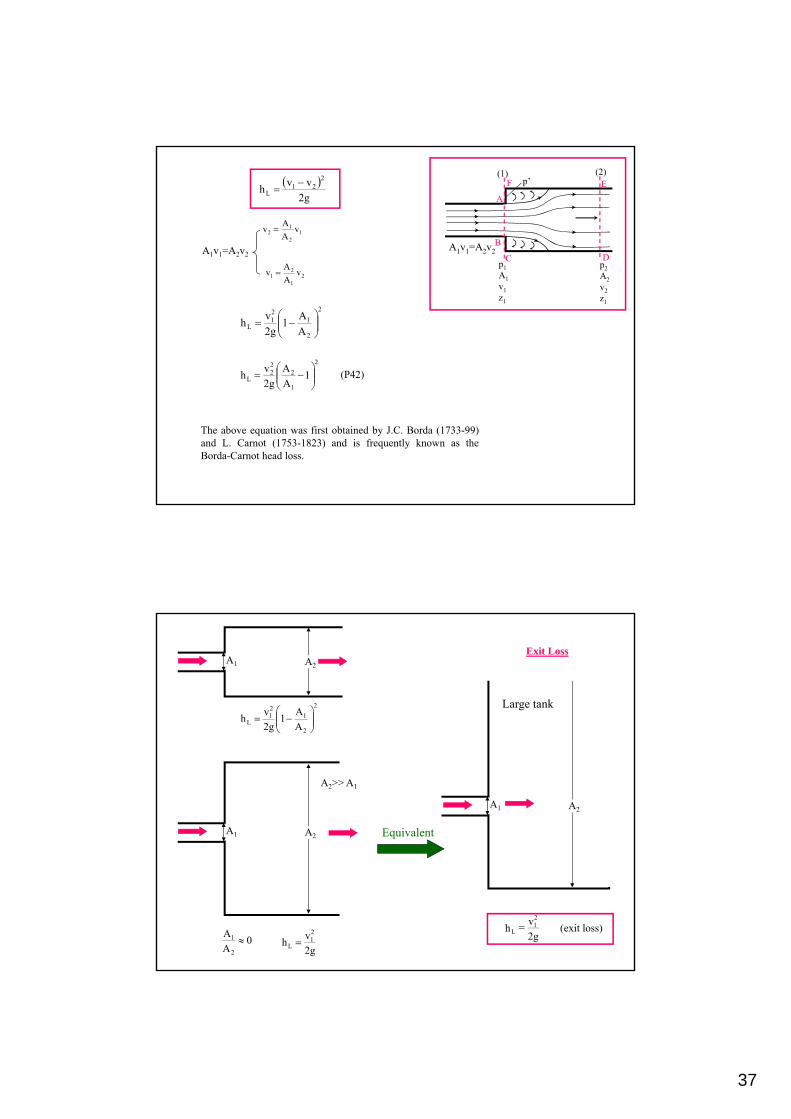
37
2
2
121
L A
A1
g2
vh
The above equation was first obtained by J.C. Borda (1733-99)and L. Carnot (1753-1823) and is frequently known as theBorda-Carnot head loss.
2
1
222
L 1A
A
g2
vh
(P42)
g2
vvh
221
L
(1) (2)p’
p1A1v1z1
p2A2v2z1
A
B
C D
EF
A1v1=A2v2
21
21 v
A
Av
A1v1=A2v2
12
12 v
A
Av
A1 A2
A2>> A1
A1 A2
2
2
121
L A
A1
g2
vh
g2
vh
21
L 0A
A
2
1
Exit Loss
A1 A2
Large tank
Equivalent
)lossexit(g2
vh
21
L

38
Vena Contracta(Area=Ac)
d2d1
Area (A1)(Section 1)
Area (A2)(Section 2)
CD
V1 V2
Figure P23
LOSS IN SUDDEN CONTRACTION
Although a SUDDEN CONTRACTION is geometrically the reverse of a SUDDEN ENLARGEMENT, it is not possible to apply the momentum equation to a control volume between sections (1) and (2).
Between the vena contracta and the downstreamsection (2) the flow pattern is similar to that after anabrupt enlargement, and the loss of head is assumedto be given by equation (P42)
2
c
22
2
c
222
L 1C
1
g2
V1
A
A
g2
Vh
Where Ac represents the cross-sectional area of vena contracta,and the coefficient of contractionCc=Ac/A2.
g2
VKh
22
scL
In general, the loss in a Sudden Contraction can be expressed as
Because of the complexity of the flow, the loss coefficient Ksc is obtained experimentally. Representative values are shown below.
d2/d1 0 0.2 0.4 0.6 0.8 1.0
Ksc 0.5 0.45 0.38 0.28 0.14 0
Note:
(a) When d2/d1=1.0, there is no sudden contraction and the pipe is a normal straight pipe, and Ksc=0.
(b) As A1 , d2/d10, the value of KSC =0.5 d2d1
g2
VKh
22
scL

39
ENTRANCE LOSS
V
K=0.5
Square-edge(flush)
V
Protrusions
(a) (b)
Figure P24
Figure P25Acknowledgment: F.M. White: Fluid Mechanics, 3rd Edition
t/d=0.02
0.04
Rounded Edge
V
Bell-mouthed
r
Figure P27
Figure P26
Acknowledgement: F.M. WhiteFluid Mechanics, 3rd Edition

40
GRADUAL EXPANSION
V1 V2
DIFFUSER
A1A2
g2
V
A
A1K
g2
VVKh
21
2
2
1L
221
LL
Energy loss can be considerably reduced if the pipe transition is more gradual.
Such a transition device is called a DIFFUSER.
Figure P29
KL
Acknowledgement: B.S. MasseyMechanics of Fluids, 3rd Edition
6o
A2/A1=4
A2/A1=2.25
9
LOSSES IN BENDS
A
BD
C
Flow separation
Flow separation
Secondary flow
Figure P30
Losses through a pipe bend = Loss due to flow separation + Loss due to friction on the wall + lossdue to secondary flow.
The loss is expressed as )46P(g2
VK
2
K depends on the total angle of the bend, surface roughness () and on the relative radius of curvature R/d, where R is the radius of curvature of the pipe centreline and d is the pipe diameter.

41
Note: (a) K is inclusive of frictional losses.(b) When R/d=0 , then K 1.1
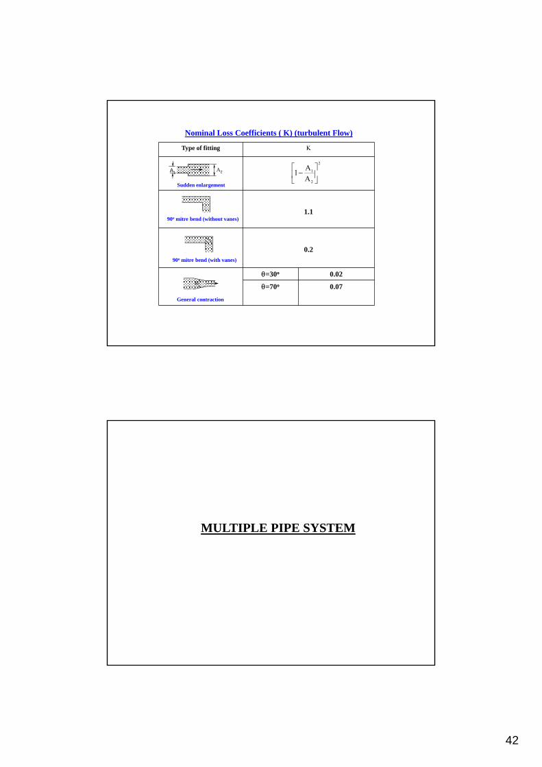
Nominal Loss Coefficients ( K) for some pipe fittings (turbulent Flow) are given in pages 182 to 184 of your lecture notes
42
Nominal Loss Coefficients ( K) (turbulent Flow)
Type of fitting K
1.1
0.2
=30o 0.02
=70o 0.07
2
2
1
A
A1
A2A1
Sudden enlargement
90o mitre bend (without vanes)
90o mitre bend (with vanes)
General contraction
MULTIPLE PIPE SYSTEM

43
Frequently, problems of dividing pipelines are encountered in engineering practice. These problems include looping pipes (pipe connected in parallel), branching pipes and pipe network
(a) Pipes connected in Series(b) Pipes connected in Parallel(c) Branched Pipes
Q1 Q2Q3
1 23
Figure P32
(a) PIPES IN SERIES
If one or more pipes are connected in series, conservation of mass gives
233
222
211 dVdVdV
Q = Q1 = Q2 = Q3 (P47)Or
The total head loss is the sum of the total losses in each of the individual pipes and fittings
HL = HL1 + HL2 + HL3 (P48)
In terms of friction and minor losses in each pipe, equation (P48) may be re-written as
ii,2
2
2222
ii,1
1
112
1L K
d
Lf
g2
VK
d
Lf
g2
VH
ii,3
3
3323 K
d
Lf
g2
V
Friction loss Minor loss

44
PIPES IN PARALLEL:
Q1
Q2
Q3
Q Q
1
2
3
(A) (B)
Figure P33
Q2
Q3
Q Q3
Q1
1
(A) (B)2
When two or more pipes are connected so that the flow divides and subsequently comes together again.
Continuity dictates that
Q = Q1 + Q2 + Q3 (P49)
At any point in the pipe, there can be only one value of total head (energy).
In other words, all fluid passing point (A) has the same total head
A
2AA zg2
V
g
P
Similarly, at point (B),
B
2BB zg2
V
g
P
LB
2BB
A
2AA Hz
g2
V
g
Pz
g2
V
g
P
The steady-energy equation may be written
Therefore, all the fluid in EACH PIPE suffer the same loss of head HL
HL1 = HL2 = HL3 (P50)
BRANCHED PIPES
Another example of practical importance involving a pipe system is when a number of pipes meeting at a junction as shown above.
The basic principles must be satisfied:
(a) Continuity: At a given junction, Mass flow rate towards the junction= Mass flow rate away from the junction.
(b) There can be only one energy level (Head) at a given point.
(c) The friction equation must be satisfied for each pipe.
Q1
Q3
z1
z2
z3
Arbitrary datum
Tank 1Tank 2
Tank 3
12
3
HJ
JQ2

45
The energy (or head) at:
(a) tank 1=H1, (b) tank 2 =H2,(c) tank 3=H3,
(d) location J = HJ
H1 - HJ = HL1 (head loss in pipe 1)H2 - HJ = HL2 (head loss in pipe 2)HJ –H3 = HL3 (head loss in pipe 3)Q3 =Q1 + Q2
Assuming that MINOR LOSSES are negligible, it can be shown that
g2
V
d
Lf
g2
V
d
Lf 23
3
3322
2
22H2-H3 = HL2 + HL3 =
g2
V
d
Lf
g2
V
d
Lf 23
3
332
1
1
11H1-H3 = HL1 + HL3 =
Under steady condition
Q1
Q3
z1
z2
z3
Arbitrary datum
Tank 1Tank 2
Tank 3
12
3
zJ
JQ2
1
2
111 z
g2
V
g
PH
2
2
222 z
g2
V
g
PH
3
2
333 z
g2
V
g
PH
J
2JJ
J zg2
V
g
PH
In general,
If P1 = P2 = P3 = Patmosphere
Assuming that tank 1, tank 2 and tank 3 are so large that
V1=V2=V3 0
If gauge pressure is used throughout, it can be shown that
11 zH
22 zH
33 zH
J
2
JJg
J zg2
V
g
PH
Q1
Q3
z1
z2
z3
Arbitrary datum
Tank 1Tank 2
Tank 3
1 2
3
HJ
JQ2
P1 P2
P3

46
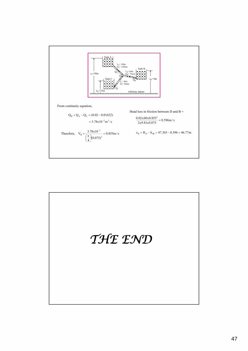
EXAMPLE 4 (page 196 of your lecture note )
Water flows from reservoir A through a 100 m long pipe of diameter 120 mm to a branch point D where it is diverted to reservoirs B and C in separate pipes as shown in the figure below. Assuming that f =0.02 for all the pipes and neglecting all losses other than those due to friction, determine the elevation of the reservoir B. The flow from the reservoir A is 0.02 m3/s.
Arbitrary datum
QA
QB
QC
zA=50m
zB=?m
Tank A
Tank C
zC=25m
LA= 100mDA= 120mm
LB= 60mDB= 75mm
Tank B
Lc= 40mDc= 60mm
D
The velocity of water between A and D is
s/m768.1)12.0(
4
10x20
A
QV
2
3
The head loss in friction between A and D is
m655.212.0x81.9x2
768.1x100x02.0
g2
V
D
fLh
22A
A
AfA
Arbitrary datum
QA
QB
QC
zA=50m
zB=?m
Tank A
Tank C
zC=25m
LA= 100mDA= 120mm
LB= 60mDB= 75mm
Tank B
Lc= 40mDc= 60mm
D
365.47655.250hzH fAAD
The head loss in friction between D and C is
365.2225365.47zH CD
.
06.0x81.9x2
xV40x02.0365.22But
2C
Therefore, VC= 5.737 m/s
Flow to reservoir C
s/m01622.0737.5x)06.0(4
32
47
Arbitrary datum
QA
QB
QC
zA=50m
zB=?m
Tank A
Tank C
zC=25m
LA= 100mDA= 120mm
LB= 60mDB= 75mm
Tank B
Lc= 40mDc= 60mm
D
s/m596.0075.0x81.9x2
855.0x60x02.0 2
m77.46596.0365.47hHz fBDB
Head loss in friction between D and B =
s/m855.0)075.0(
4
10x78.3V,Therefore
2
3
B
From continuity equation,
)01622.002.0(QQQ CAB
s/m10x78.3 33
THE END


