480
ME445 FINAL PROJECT REPORT ELECTRONIC KEYBOARD Department of Mechanical and Nuclear Engineering The Pennsylvania State University Submitted by: Thomas Burke Chris Guarracino May 3, 2013

ME445
FINAL PROJECT REPORT ELECTRONIC KEYBOARD Department of Mechanical and Nuclear Engineering The Pennsylvania State University
Submitted by: Thomas Burke Chris Guarracino May 3, 2013

1
Table of Contents Introduction.................................................................................................................................................... 2
Bill of Materials .............................................................................................................................................. 2
Hardware Components ................................................................................................................................. 2
Arduino Mega ............................................................................................................................................ 2
Musical Instrument Shield ......................................................................................................................... 3
4 x 4 Keypad .............................................................................................................................................. 3
Piezoelectric Discs .................................................................................................................................... 4
Serial LCD ................................................................................................................................................. 4
7 Segment LED Display ............................................................................................................................ 5
Circuit Diagram ............................................................................................................................................. 5
Software Components ................................................................................................................................... 6
Electrical Components - Detail ...................................................................................................................... 7
Design Evolution ......................................................................................................................................... 10
Problems ..................................................................................................................................................... 11
Features ...................................................................................................................................................... 12
Conclusions and Future Recommendations ............................................................................................... 14
Appendices ................................................................................................................................................. 15
Appendix A: Arduino Code ...................................................................................................................... 15
Appendix B: References .......................................................................................................................... 46
Appendix C: Spec Sheets........................................................................................................................ 47

2
Introduction The objective of this report was to create a user-friendly device capable of playing music based
off of an operator’s commands. From the beginning, we knew that we wanted a project that
relied heavily on user interaction. We decided to venture down the path of music, based on our
mutual interest of learning and playing musical instruments.
The Arduino in combination with the Musical Instrument Shield and piezodiscs are the three
main components in this project. When the piezodiscs are distorted in tension or compression, a
note is played through a speaker and displayed on a 7-segment-LED display.
Playing music with the apparatus is very similar to using an electric keyboard. The only
difference is, instead of pressing keys with your fingers, keys are hit with a mallet. The keys
could have been made of any material, due to the resourcefulness of the piezodiscs. The sound
library of the Musical Instrument shield is extensive. The user has the option of selecting one of
128 instruments and playing the standard major scale of low C to high C.
Bill of Materials
Material Model # Vendor Qty Cost
Arduino Mega 2560 R3 ME445 Lab 1 FREE
Musical Instrument Shield DEV-10587 SparkFun 1 $30.95
4 x 4 Keypad AK-1607 ME445 Lab 1 FREE
1/8" Lexan N/A ME445 Lab 12" X 12" FREE
Piezoelectric disc B00A9AMHTI Audiowell 15 $15.49
Total $56.12
As seen in the table above, the costs of this project come out to be $56.12. This total is fairly
inexpensive, compared with other projects. One attributing factor for this low cost is that the
Arduino Mega, Lexan, and keypad were provided for free by the lab. A wooden frame and
various resistors were also a part of this project, but not included in the Bill of Materials. The
frame that houses the Lexan keys could be of any geometry, made out of any rigid material.
Hardware Components This project combined an equal mix of electrical and mechanical parts to produce music.
Arduino Mega An Arduino Mega was used for this project, because of its numerous number of pins. The
Arduino Uno only has 14 digital input/outpus pins and 6 analog inputs, compared to the Arduino
Mega’s 64 digital input/output pins and 16 analog inputs.

3
Figure 1 Image of Arduino MEGA
Musical Instrument Shield The Musical Instrument Shield was the brains of the code that handled processes the Arduino
Mega could not. The shield is made to fit directly on top of the Arduino upon the soldering of
four headers.
Figure 2 Image of Musical Instrument Shield
4 x 4 Keypad An AK-1607 4x4 keypad is used as the device which determines the current instrument. To
choose an instrument from the library, a user types in “*”, then the identification number of the
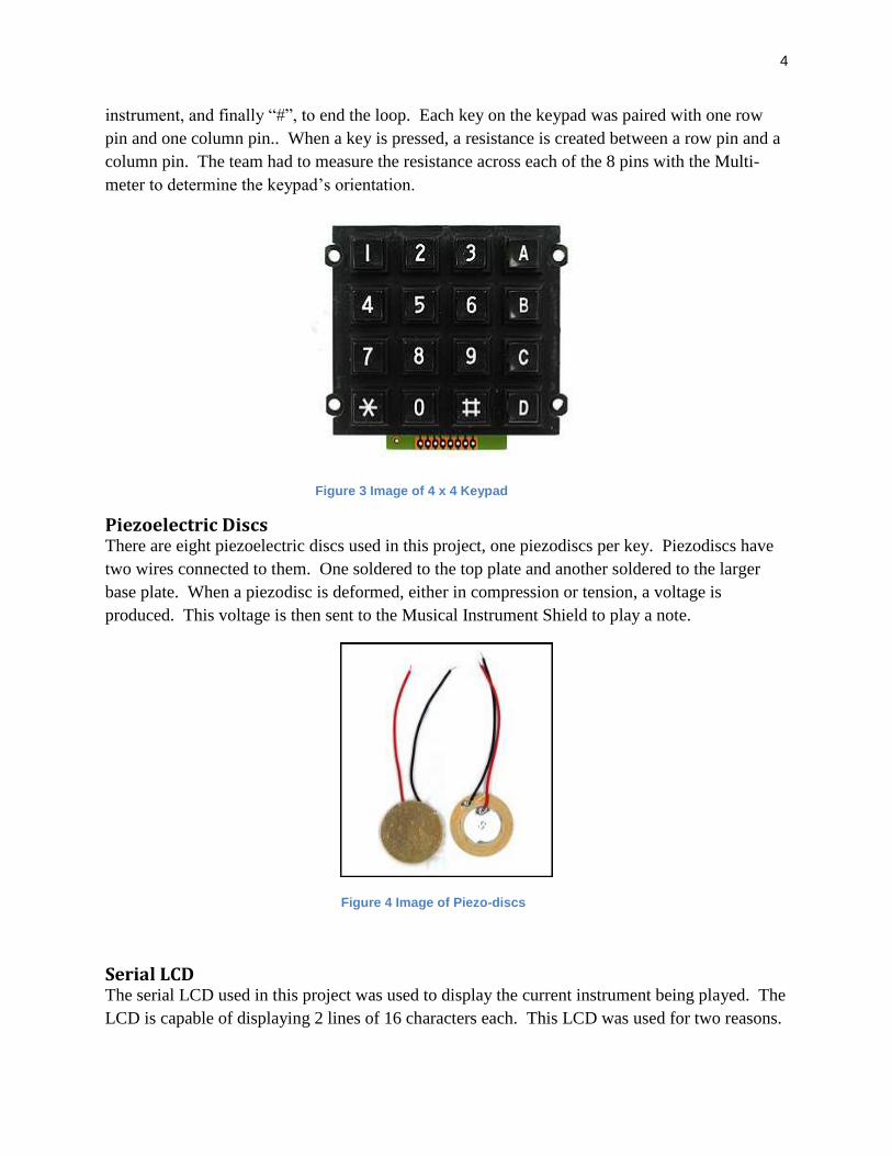
4
instrument, and finally “#”, to end the loop. Each key on the keypad was paired with one row
pin and one column pin.. When a key is pressed, a resistance is created between a row pin and a
column pin. The team had to measure the resistance across each of the 8 pins with the Multi-
meter to determine the keypad’s orientation.
Figure 3 Image of 4 x 4 Keypad
Piezoelectric Discs There are eight piezoelectric discs used in this project, one piezodiscs per key. Piezodiscs have
two wires connected to them. One soldered to the top plate and another soldered to the larger
base plate. When a piezodisc is deformed, either in compression or tension, a voltage is
produced. This voltage is then sent to the Musical Instrument Shield to play a note.
Figure 4 Image of Piezo-discs
Serial LCD The serial LCD used in this project was used to display the current instrument being played. The
LCD is capable of displaying 2 lines of 16 characters each. This LCD was used for two reasons.

5
Firstly, it is very easy to set up, because it only requires three connections. Some LCDs require
at least nine wires to be soldered to it. Secondly, this LCD was very easy to use. Code was
taken from a previous lab and allowed us to have the display working almost instantly.
Figure 5 Image of Serial LCD Display
7 Segment LED Display We used a 7-segment display to show the last note that the user played. This display is a useful
tool for those who cannot distinguish different musical notes by ear. Our 7 segment display had
10 pins. Two pins went to ground and eight pins went to resistors in series with the Arduino.
The eight pins that went to the Arduino were what determined which segment lit up. This is
further explained below, in Figure 9.
Figure 6 Image of 7 Segment LED Display
Circuit Diagram The Fritzing program was used to create a clean looking circuit diagram of the whole system. Since the piezo discs that we used were not in the Fritzing library, we instead modeled the piezo discs by using black force sensors.
LCD display box
white
red
black
TX > 1
GND
5V

6
Figure 7 Circuit Diagram
Software Components The code for the keyboard was written using the Arduino compiler provided on the PCs in 339
Reber. Roughly half of the code was original and the other half was taken from the public
domain. Most notably, the code used to initialize Musical Instrument Shield was taken from the
examples provided on Spark Fun’s website. The majority of the code is included in functions
that either call each other or get called inside the main for loop. Our main program initializes all
the variables and the pins on the Arduino Mega for communication as well as prepares the LCD
box for full functionality. We have a total of 14 different functions for our program. Eight of

7
these functions control the 7-segment LCD display where each function lights up different LEDs
so that the 7-segment component can display the appropriate note when a key is pressed. Two of
these functions, called ballgame( ) and classical( ), tell the Arduino to play built-in songs. Inside
these song functions is repetitive code that cycles through the notes of a given song, say Take Me
Out to the Ballgame. The code turns notes on and off and varies the delay between notes in an
effort to match the appropriate beat. Another function, called getKey( ), is used to get the key
from the 16 button Spark Fun keypad. Our code uses a two dimensional array to hold the values
of the keypad as chars. Working with this function is another, called threeDigits( ), that is
capable of combining multiple key presses into either a 1, 2, or 3 digit number. This was crucial
to our project since the musical instrument shield offers well over 100 different sounds. We
wanted to use that component to its full potential so our user would have maximum functionality.
A function called instrumentSetter( ) takes the number produced by threeDigits( ) and matches it
to the corresponding instrument tones built into the musical instrument shield. It also tells the
LCD box to display the name of the instrument for the user to see. Lastly, the function
playOctave( ), makes the keyboard actually produce sounds. It contains a loop that constantly
looks for which of the 8 keys is pressed, and tells the Arduino and Musical Instrument Shield to
play the appropriate note henceforth.
Electrical Components - Detail We dedicated a significant amount of time and troubleshooting to fully understand the operations
of the 4x4 keypad. Figure 8 shows the inside layout of the keypad. This information helped our
team learn which buttons closed which circuits and which combination of output pins from the
keypad we should use. For example, pressing number 6 would result in row 2 and column 3
being engaged. This row and column correspond to output pins 2 and 6, respectively. If one
were to take a multimeter and measure the resistance across those two pins when 6 is pushed, the
resistance would be approximately 0 ohms. The code that gets the key pressed from the keypad
cycles through a loop that looks for when the input pins read LOW. This means that a button
was pressed because the circuit is now closed. A 2x2 char array is used to reference which
number/letter was pressed based off of the input to the Arduino Mega pins.

8
Figure 8 Specification Overview of Keypad

9
Figure 9 Labeled 7 Segment LED Display
In order for the difference segments to light up, each pin needs to receive a HIGH signal from
the Arduino. We connected this display to the digital output pins on our Arduino Mega and
wrote code for each of the letters for the music octave scale: C D E F G A B C. We have 8
different functions that get called in our program that cycle through the A→H LEDs in order to
display the appropriate note.
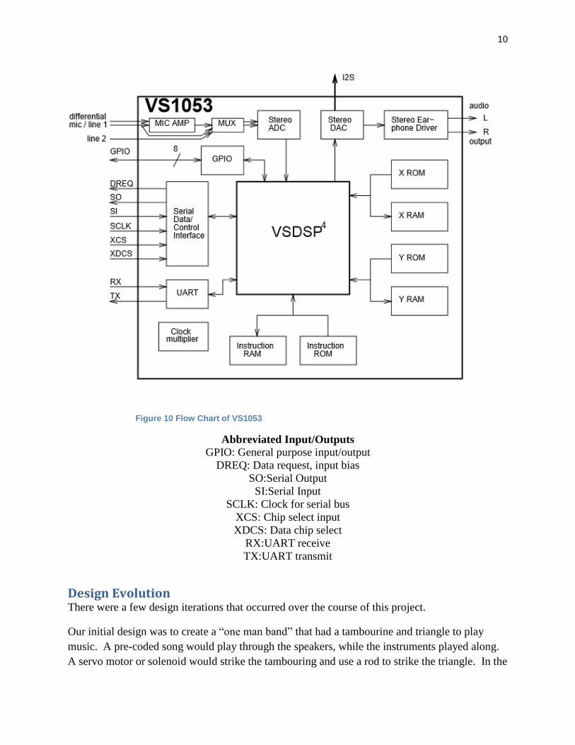
The main component of the Musical Instrument Shield is the VS1053 MP3 and MIDI codec IC,
wired in MIDI mode. The VS1053 is what stores the Melodic Instruments and Percussion
Instruments sound banks, seen in Figure 11 below. The shield will allow for a sound output
while the Arduino runs processes simultaneously. Figure 10, directly below, is a flow chart
describing the VS1053’s processes. As the central hub, the VSDSP is a low power, 16/320bit
DSP processor core. The internal clock operates at 12-13 MHz for standard processes and has
the option of increasing to 24-26 MHz.
10
Figure 10 Flow Chart of VS1053
Abbreviated Input/Outputs
GPIO: General purpose input/output
DREQ: Data request, input bias
SO:Serial Output
SI:Serial Input
SCLK: Clock for serial bus
XCS: Chip select input
XDCS: Data chip select
RX:UART receive
TX:UART transmit
Design Evolution There were a few design iterations that occurred over the course of this project.
Our initial design was to create a “one man band” that had a tambourine and triangle to play
music. A pre-coded song would play through the speakers, while the instruments played along.
A servo motor or solenoid would strike the tambouring and use a rod to strike the triangle. In the

11
early stages, these were the only instruments that were considered and they did not perform well.
The low quality properties of the tambourine led to a poor sound when struck by the solenoid.
This led us to transition into a system that did not use these instruments.
Next, we tried to transition into a design that utilized the Musical Instrument Shield more. In the
previous design, we were only using the shield to play a pre-coded song. The Musical
Instrument Shield however, had great features that were not being employed.
Finally, we came up with a design that allowed the user to play their own notes, instead of
programming in a song. This design utilizes 8 piezo discs for the major C scale (hepatonic scale)
for the top bank of melodic instruments and 5 piezo discs for the bottom bank of percussion
instruments.
Problems We originally had many difficulties using the Musical Instrument Shield. The connection pins
wouldn’t make good contact with the Arduino’s pins and therefore the power supplied to the
shield wasn’t always what it needed to run. This caused it to malfunction. Soldering the
connectors to the shield solved this problem. Also, we had difficulties with the volume of the
sound coming from the shield. Since we didn’t have an external speaker to plug into the shield
nearer to the beginning of our project, we had to use our headphones. Needless to say, the sound
level coming from the shield was very low and difficult to hear. Extensive research online
taught us the line of code we had to modify to boost the volume level. This problem was then
quickly solved by modifying the following line: talkMIDI(0xC0,instrumentchoice,XX). XX is a
number from 0 to 127 corresponding to volume level, where 127 is the maximum volume level.
The piezo discs provided more frustration than any other component used in our project. The
problem plaguing our team from the beginning of the project was the sensitivity of the discs.
This did not seem to stay uniform throughout our testing. One day, a light strike of the disc
would produce the desired result. Another day would require a forceful strike to achieve the
same results. The second problem was the frail nature of the hardwired connection cables from
the discs. Not only were they extremely small and difficult to solder to another, thicker wire; but
they could easily come disconnected from the disc. By the final week of the semester, however,

12
these problems were solved with a little common sense. The variable striking force problem was
corrected by changing the length and thickness of the keyboard’s “keys”. Originally we had 4”
long and 3/16” thick Lexan keys. The final keyboard now uses 7” long and 1/8” thick keys.
Changing these dimensions improved the reliability and functionality of our piezo disc –
powered keyboard keys. Lastly, removing the original wires from the piezo discs and directly
soldering thicker wire provided in the lab to the disc’s surface bolstered the strength of our
connections.
The software (coded included in Appendix) had numerous problems throughout the course of the
semester. Standard debugging weeded out these problems, as well as soliciting Mike’s help
when needed. The final code included in this report is the cleanest iteration our team has
produced. As a side note, there seems to be some error with some of the built-in instruments of
the Musical Instrument Shield. Some instrument selections do not produce any sound at all. The
code that is responsible for this is identical for all instruments, excluding the line that tells the
shield what instrument to play: talkMIDI(0xC0, xx, 0). The “xx” parameter corresponds to the
instrument number. Roughly 95% of the 128 melodic instruments generate sounds.
Features To utilize the full functionality of the keyboard, users must familiarize themselves with the page
from the datasheet as seen in Figure 11. Our Arudino and Musical Instrument Shield can
produce 128 different sounds for a melody. Users have access to all of these sounds through the
provided keypad. To change the instrument that the keyboard plays, users simply enter a 1, 2, or
3 digit number on the keypad in the pattern as follows: Press * to initialize the listener, enter a 1,
2, or 3 digit number corresponding to the desired instrument, press # to terminate the sequence.
In our keyboard, the # button acts as an enter key for the user to send the number they entered
into the Arduino for processing. An LCD box is included with the keyboard to provide visual
confirmation that the user is getting the instrument they requested. The box will display the
name of the current instrument for the user to see. The keyboard also has two built in songs for
users to play, which we included in the 200-300 number banks. Users simply enter in numbers
200 or 201 to hear the keyboard play its own tune. On the educational side, the 7-segment LED
display helps to educate the user as to what note they are playing on the keyboard. Whenever a
key is stuck, the 7-segment display shows the corresponding note, whether it be a D, B, E, etc.
This display changes on its own from key to key and does not require any other inputs from the
user other than playing the keyboard.

13
Figure 11 List of Available Instruments

14
Conclusions and Future Recommendations Our final product offers numerous entertaining and educational features for users of all ages.
The ability to choose over 100 different instruments allows users the flexibility to be creative
with the music they create. Additionally, beginners will be able to learn about the octave scale
and can start to identify notes based on the sound they hear. The 7-segmet LCD was chosen to
display this so that it would be an attention grabber because it resembles the displays people see
at exciting places like sporting events. The next generation of this keyboard will allow users to
play a song on the keys and have the Arduino store it and save it to a PC for future use.
Additional components will be needed to make this a reality, but our team feels that such a
feature will be highly regarded by consumers.

15
Appendices
Appendix A: Arduino Code
#include <SoftwareSerial.h>
SoftwareSerial mySerial(2, 3); // RX, TX
byte note = 0; //The MIDI note value to be played
byte resetMIDI = 4; //Tied to VS1053 Reset line
byte ledPin = 13; //MIDI traffic inidicator
int a = 0;
//Set up keypad params
const int numRows = 4; // number of rows in the keypad
const int numCols = 4; // number of columns
const int debounceTime = 20; // number of milliseconds for switch to be
stable
// keymap defines the character returned when the corresponding key is presse
d
const char keymap[numRows][numCols] =
'1', '2', '3' , 'A' ,
'4', '5', '6' , 'B' ,
'7', '8', '9' , 'C' ,
'*', '0', '#' , 'D'
;
// this array determines the pins used for rows and columns
const int rowPins[numRows] = 50, 48, 46, 44; // Rows 0 through 3
const int colPins[numCols] = 42, 40, 38, 36 ; // Columns 0 through 2
const int bank_change = 8; // Pin read that allows users to change from the
medolic bank to the percussive bank
int instrumentChoice; // Stores the three digit number corresponding to the
instrument on the sheld's data sheet
int baseball = 9; // Pin to control "Take Me Out to the Ballgame"
int classicalPin = 13; // Pin to Control Bach song
int instrument = 0;
int threshold = 20;
int buttonOn = 0;
int buttonOff = 0;
int counter1 = 0;
int counter2 = 0;
int played = 0;
byte LCD_reset = 12; // reset LCD, clear screen and move to line 0,
position 0
byte LCD_line0 = 128; // LCD set line 0, character 0
byte LCD_line1 = 148; // LCD set line 1, character 0
void setup()
Serial.begin(9600);

16
//For Keypad
for (int row = 0; row < numRows; row++)
pinMode(rowPins[row],INPUT); // Set row pins as input
digitalWrite(rowPins[row],HIGH); // turn on Pull-ups
for (int column = 0; column < numCols; column++)
pinMode(colPins[column],OUTPUT); // Set column pins as outputs
// for writing
digitalWrite(colPins[column],HIGH); // Make all columns inactive
//Setup soft serial for MIDI control
mySerial.begin(31250);
//Reset the VS1053
pinMode(resetMIDI, OUTPUT);
digitalWrite(resetMIDI, LOW);
delay(100);
digitalWrite(resetMIDI, HIGH);
delay(100);
talkMIDI(0xB0, 0x07, 127); //0xB0 is channel message, set channel volume to
near max (127)
//Clear out the LCD and prepare for business
setupLCD();
//Initialize the pins for the keypad
pinMode(31, OUTPUT);
pinMode(33, OUTPUT);
pinMode(35, OUTPUT);
pinMode(37, OUTPUT);
pinMode(39, OUTPUT);
pinMode(41, OUTPUT);
pinMode(43, OUTPUT);
pinMode(45, OUTPUT);
pinMode(bank_change,INPUT);
pinMode(baseball,INPUT);
pinMode(classicalPin,INPUT);
talkMIDI(0xB0, 0, 0x00); // Bank select melodic instruments
void loop()
//Default bank GM1
// Listen for numbers pressed by user on keypad.
if (getKey() != 0)
instrumentChoice = threeDigits(); // Store three digit instrument number
into instrument choice
instrumentSetter(); //Take the three digit number and set the instrument
tone for the shield to play
playOctave(); // Listens for a key press and plays corresponding note

17
//Send a MIDI note-on message. Like pressing a piano keyW
void noteOn(byte channel, byte note, byte attack_velocity)
talkMIDI( (0x90 | channel), note, attack_velocity);
//Send a MIDI note-off message. Like releasing a piano key
void noteOff(byte channel, byte note, byte release_velocity)
talkMIDI( (0x80 | channel), note, release_velocity);
//Plays a MIDI note. Doesn't check to see that cmd is greater than 127, or th
at data values are less than 127
void talkMIDI(byte cmd, byte data1, byte data2)
digitalWrite(ledPin, HIGH);
mySerial.write(cmd);
mySerial.write(data1);
//Some commands only have one data byte. All cmds less than 0xBn have 2
data bytes
//(sort of: http://253.ccarh.org/handout/midiprotocol/)
if( (cmd & 0xF0) <= 0xB0)
mySerial.write(data2);
digitalWrite(ledPin, LOW);
// Plays take me out to the ball game
void writeA()
digitalWrite(43, 1);
digitalWrite(41, 1);
digitalWrite(35, 1);
digitalWrite(33, 1);
digitalWrite(39, 1);
digitalWrite(37, 1);
digitalWrite(31, 1);
digitalWrite(45, 0);
void writeB()
digitalWrite(43, 1);
digitalWrite(41, 1);
digitalWrite(35, 1);
digitalWrite(33,0);
digitalWrite(39, 1);
digitalWrite(37, 1);
digitalWrite(31, 0);
digitalWrite(45, 1);
void writeC()
digitalWrite(43, 1);
digitalWrite(41, 0);
18
digitalWrite(35, 1);
digitalWrite(33, 1);
digitalWrite(39, 0);
digitalWrite(37, 0);
digitalWrite(31, 0);
digitalWrite(45, 1);
void writeMiddleC()
digitalWrite(43, 1);
digitalWrite(41, 0);
digitalWrite(35, 1);
digitalWrite(33,1);
digitalWrite(39, 1);
digitalWrite(37, 0);
digitalWrite(31, 0);
digitalWrite(45, 1);
void writeD()
digitalWrite(43, 1);
digitalWrite(41, 1);
digitalWrite(35, 0);
digitalWrite(33,0);
digitalWrite(39, 0);
digitalWrite(37, 1);
digitalWrite(31, 1);
digitalWrite(45, 1);
void writeE()
digitalWrite(33,1);
digitalWrite(45,1);
digitalWrite(37,1);
digitalWrite(35,1);
digitalWrite(43,1);
digitalWrite(39,0);
digitalWrite(41,0);
digitalWrite(31,0);
void writeF()
digitalWrite(33,1);
digitalWrite(45,0);
digitalWrite(37,1);
digitalWrite(35,1);
digitalWrite(43,1);
digitalWrite(39,0);
digitalWrite(41,0);
digitalWrite(31,0);

19
void writeG()
digitalWrite(33,1);
digitalWrite(45,1);
digitalWrite(37,1);
digitalWrite(35,1);
digitalWrite(43,0);
digitalWrite(39,0);
digitalWrite(41,1);
digitalWrite(31,1);
void setupLCD()
Serial.write( LCD_reset );
Serial.print( " " );
Serial.write( LCD_line1 );
Serial.print( " " );
//function takes the possibe inputs from the user and converts them to the ap
propriate insturment
// for the musical insturment shield Lost of repetitive code here, so we wil
l comment on iteration only
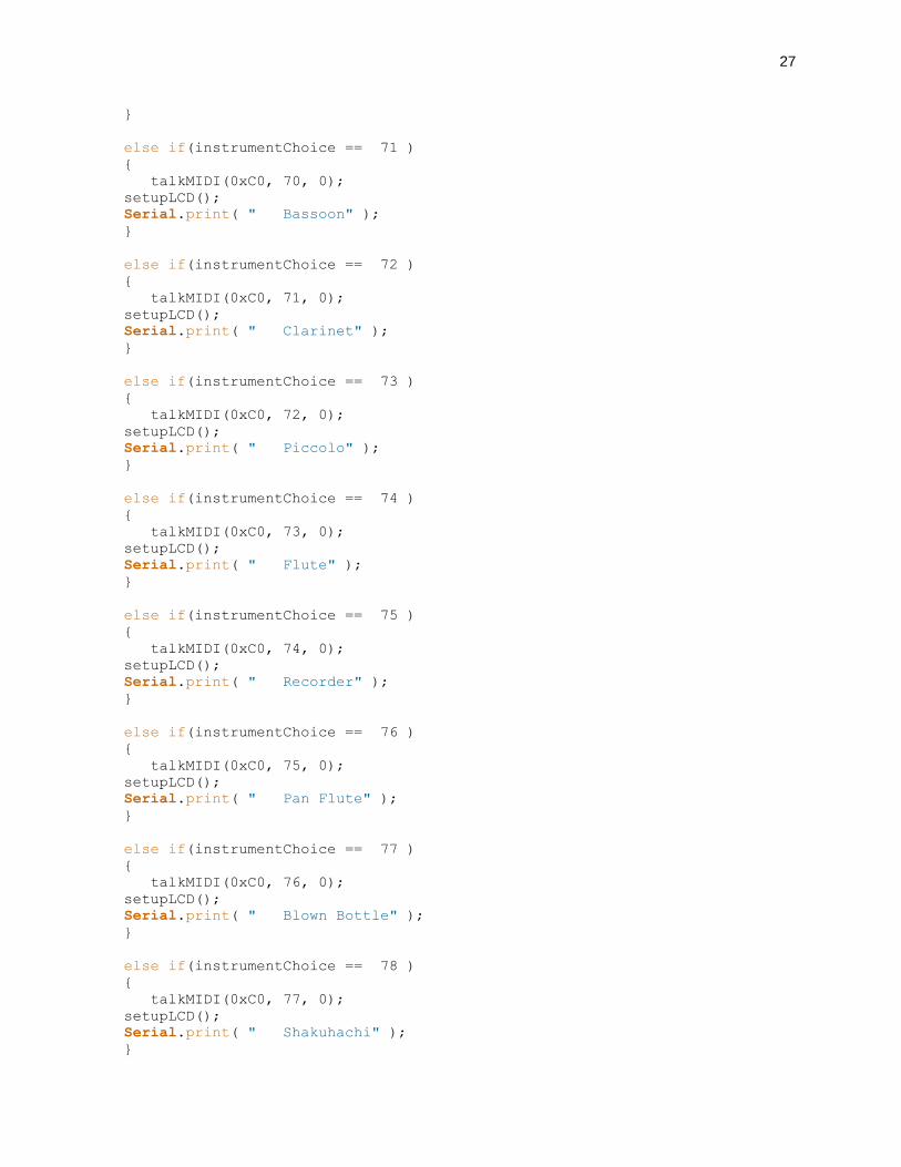
void instrumentSetter()
if(instrumentChoice == 1) // if user chooses "grand piano" whose number = 1
talkMIDI(0xC0, 0, 0); //Sets the instrument on the Shield - grand piano
setupLCD(); //Clear LCD
Serial.print( " Grand Piano" ); //Write the instrument name to the LCD
else if(instrumentChoice == 2)
talkMIDI(0xC0, 1, 0);
setupLCD();
Serial.print( " Bright Piano" );
else if(instrumentChoice == 3)
talkMIDI(0xC0, 2, 0);
setupLCD();
Serial.print( " Electric Grand Piano" );
else if(instrumentChoice == 4)
talkMIDI(0xC0, 3, 0);
setupLCD();
Serial.print( " Honky-tonk Piano" );
else if(instrumentChoice == 5)
talkMIDI(0xC0, 4, 0);
setupLCD();

20
Serial.print( " Electric Piano 1" );
else if(instrumentChoice == 6)
talkMIDI(0xC0, 5, 0);
setupLCD();
Serial.print( " Electric Piano 2" );
else if(instrumentChoice == 7)
talkMIDI(0xC0, 6, 0);
setupLCD();
Serial.print( " Harpsichord" );
else if(instrumentChoice == 8)
talkMIDI(0xC0, 7, 0);
setupLCD();
Serial.print( " Clavi" );
else if(instrumentChoice == 9)
talkMIDI(0xC0, 8, 0);
setupLCD();
Serial.print( " Celesta" );
else if(instrumentChoice == 10)
talkMIDI(0xC0, 9, 0);
setupLCD();
Serial.print( " Glockenspiel" );
else if(instrumentChoice == 11)
talkMIDI(0xC0, 10, 0);
setupLCD();
Serial.print( " Music Box" );
else if(instrumentChoice == 12)
talkMIDI(0xC0, 11, 0);
setupLCD();
Serial.print( " Vibraphone" );
else if(instrumentChoice == 13)
talkMIDI(0xC0, 12, 0);
setupLCD();
Serial.print( " Marimba" );
else if(instrumentChoice == 14)
talkMIDI(0xC0, 13, 0);
setupLCD();
Serial.print( " Xylophone" );

21
else if(instrumentChoice == 15)
talkMIDI(0xC0, 14, 0);
setupLCD();
Serial.print( " Tubular Bells" );
else if(instrumentChoice == 16)
talkMIDI(0xC0, 15, 0);
setupLCD();
Serial.print( " Dulcimer" );
else if(instrumentChoice == 17)
talkMIDI(0xC0, 16, 0);
setupLCD();
Serial.print( " Drawbar Organ" );
else if(instrumentChoice == 18)
talkMIDI(0xC0, 17, 0);
setupLCD();
Serial.print( " Percussive Organ" );
else if(instrumentChoice == 19)
talkMIDI(0xC0, 18, 0);
setupLCD();
Serial.print( " Rock Organ" );
else if(instrumentChoice == 20)
talkMIDI(0xC0, 19, 0);
setupLCD();
Serial.print( " Church Organ" );
else if(instrumentChoice == 21)
talkMIDI(0xC0, 20, 0);
setupLCD();
Serial.print( " Reed Organ" );
else if(instrumentChoice == 22)
talkMIDI(0xC0, 21, 0);
setupLCD();
Serial.print( " Accordian" );
else if(instrumentChoice == 23)
talkMIDI(0xC0, 22, 0);
setupLCD();
Serial.print( " Harmonica" );
else if(instrumentChoice == 24)
talkMIDI(0xC0, 23, 0);

22
setupLCD();
Serial.print( " Tango Accordian" );
else if(instrumentChoice == 25)
talkMIDI(0xC0, 24, 0);
setupLCD();
Serial.print( " Acoustic Guitar (nylon)" );
else if(instrumentChoice == 26)
talkMIDI(0xC0, 25, 0);
setupLCD();
Serial.print( " Acoutic Guitar (steel)" );
else if(instrumentChoice == 27)
talkMIDI(0xC0, 26, 0);
setupLCD();
Serial.print( " Elextric Guitar (jazz)" );
else if(instrumentChoice == 28)
talkMIDI(0xC0, 27, 0);
setupLCD();
Serial.print( " Electric Guitar (clean)" );
else if(instrumentChoice == 29)
talkMIDI(0xC0, 28, 0);
setupLCD();
Serial.print( " Electric Guitar (muted)" );
else if(instrumentChoice == 30)
talkMIDI(0xC0, 29, 0);
setupLCD();
Serial.print( " Overdriven Guitar" );
else if(instrumentChoice == 31)
talkMIDI(0xC0, 30, 0);
setupLCD();
Serial.print( " Distortion Guitar" );
else if(instrumentChoice == 32)
talkMIDI(0xC0, 31, 0);
setupLCD();
Serial.print( " Guitar Harmonics" );
else if(instrumentChoice == 33)
talkMIDI(0xC0, 32, 0);
setupLCD();
Serial.print( " Acoustic Bass" );

23
else if(instrumentChoice == 34)
talkMIDI(0xC0, 33, 0);
setupLCD();
Serial.print( " Electric Bass (finger)" );
else if(instrumentChoice == 35)
talkMIDI(0xC0, 34, 0);
setupLCD();
Serial.print( " Electric Bass (pick)" );
else if(instrumentChoice == 36)
talkMIDI(0xC0, 35, 0);
setupLCD();
Serial.print( " Fretless Bass" );
else if(instrumentChoice == 37)
talkMIDI(0xC0, 36, 0);
setupLCD();
Serial.print( " Slap Bass 1" );
else if(instrumentChoice == 38)
talkMIDI(0xC0, 37, 0);
setupLCD();
Serial.print( " Slap Bass 2" );
else if(instrumentChoice == 39)
talkMIDI(0xC0, 38, 0);
setupLCD();
Serial.print( " Synth Bass 1" );
else if(instrumentChoice == 40)
talkMIDI(0xC0, 39, 0);
setupLCD();
Serial.print( " Synth Bass 2" );
else if(instrumentChoice == 41)
talkMIDI(0xC0, 40, 0);
setupLCD();
Serial.print( " Violin" );
else if(instrumentChoice == 42)
talkMIDI(0xC0, 41, 0);
setupLCD();
Serial.print( " Viola" );
else if(instrumentChoice == 43)
24
talkMIDI(0xC0, 42, 0);
setupLCD();
Serial.print( " Cello" );
else if(instrumentChoice == 44)
talkMIDI(0xC0, 43, 0);
setupLCD();
Serial.print( " Contrabass" );
else if(instrumentChoice == 45)
talkMIDI(0xC0, 44, 0);
setupLCD();
Serial.print( " Tremolo Strings" );
else if(instrumentChoice == 46)
talkMIDI(0xC0, 45, 0);
setupLCD();
Serial.print( " Pizzicato Strings" );
else if(instrumentChoice == 47)
talkMIDI(0xC0, 46, 0);
setupLCD();
Serial.print( " Orchestral Harp" );
else if(instrumentChoice == 48)
talkMIDI(0xC0, 47, 0);
setupLCD();
Serial.print( " Timpani" );
else if(instrumentChoice == 49)
talkMIDI(0xC0, 48, 0);
setupLCD();
Serial.print( "String Ensembles 1" );
else if(instrumentChoice == 50)
talkMIDI(0xC0, 49, 0);
setupLCD();
Serial.print( " String Ensembles 2" );
else if(instrumentChoice == 51)
talkMIDI(0xC0, 50, 0);
setupLCD();
Serial.print( " Synth Strings 1" );
else if(instrumentChoice == 52)
talkMIDI(0xC0, 51, 0);
setupLCD();
Serial.print( " Synth Strings 2" );

25
else if(instrumentChoice == 53)
talkMIDI(0xC0, 52, 0);
setupLCD();
Serial.print( " Choir Aahs" );
else if(instrumentChoice == 54)
talkMIDI(0xC0, 53, 0);
setupLCD();
Serial.print( " Voice Oohs" );
else if(instrumentChoice == 55)
talkMIDI(0xC0, 54, 0);
setupLCD();
Serial.print( " Synth Voice" );
else if(instrumentChoice == 56)
talkMIDI(0xC0, 55, 0);
setupLCD();
Serial.print( " Orhestra Hit" );
else if(instrumentChoice == 57)
talkMIDI(0xC0, 56, 0);
setupLCD();
Serial.print( " Trumpet" );
else if(instrumentChoice == 58)
talkMIDI(0xC0, 57, 0);
setupLCD();
Serial.print( " Trombone" );
else if(instrumentChoice == 59)
talkMIDI(0xC0, 58, 0);
setupLCD();
Serial.print( " Tuba" );
else if(instrumentChoice == 60)
talkMIDI(0xC0, 59, 0);
setupLCD();
Serial.print( " Muted Trumpet" );
else if(instrumentChoice == 61)
talkMIDI(0xC0, 60, 0);
setupLCD();
Serial.print( " French Horn" );
else if(instrumentChoice == 62)

26
talkMIDI(0xC0, 61, 0);
setupLCD();
Serial.print( " Brass Section" );
else if(instrumentChoice == 63)
talkMIDI(0xC0, 62, 0);
setupLCD();
Serial.print( " Synth Brass 1" );
else if(instrumentChoice == 64)
talkMIDI(0xC0, 63, 0);
setupLCD();
Serial.print( " Synth Brass 2" );
else if(instrumentChoice == 65 )
talkMIDI(0xC0, 64, 0);
setupLCD();
Serial.print( " Soprano Sax" );
else if(instrumentChoice == 66 )
talkMIDI(0xC0, 65, 0);
setupLCD();
Serial.print( " Alto Sax" );
else if(instrumentChoice == 67 )
talkMIDI(0xC0, 66, 0);
setupLCD();
Serial.print( " Tenor Sax" );
else if(instrumentChoice == 68 )
talkMIDI(0xC0, 67, 0);
setupLCD();
Serial.print( " Baritone Sax" );
else if(instrumentChoice == 69 )
talkMIDI(0xC0, 68, 0);
setupLCD();
Serial.print( " Oboe" );
else if(instrumentChoice == 70 )
talkMIDI(0xC0, 69, 0);
setupLCD();
Serial.print( " English Horn" );
27
else if(instrumentChoice == 71 )
talkMIDI(0xC0, 70, 0);
setupLCD();
Serial.print( " Bassoon" );
else if(instrumentChoice == 72 )
talkMIDI(0xC0, 71, 0);
setupLCD();
Serial.print( " Clarinet" );
else if(instrumentChoice == 73 )
talkMIDI(0xC0, 72, 0);
setupLCD();
Serial.print( " Piccolo" );
else if(instrumentChoice == 74 )
talkMIDI(0xC0, 73, 0);
setupLCD();
Serial.print( " Flute" );
else if(instrumentChoice == 75 )
talkMIDI(0xC0, 74, 0);
setupLCD();
Serial.print( " Recorder" );
else if(instrumentChoice == 76 )
talkMIDI(0xC0, 75, 0);
setupLCD();
Serial.print( " Pan Flute" );
else if(instrumentChoice == 77 )
talkMIDI(0xC0, 76, 0);
setupLCD();
Serial.print( " Blown Bottle" );
else if(instrumentChoice == 78 )
talkMIDI(0xC0, 77, 0);
setupLCD();
Serial.print( " Shakuhachi" );

28
else if(instrumentChoice == 79 )
talkMIDI(0xC0, 78, 0);
setupLCD();
Serial.print( " Whistle" );
else if(instrumentChoice == 80 )
talkMIDI(0xC0, 79, 0);
setupLCD();
Serial.print( " Ocarina" );
else if(instrumentChoice == 81 )
talkMIDI(0xC0, 80, 0);
setupLCD();
Serial.print( " Square Lead" );
else if(instrumentChoice == 82 )
talkMIDI(0xC0, 81, 0);
setupLCD();
Serial.print( " Saw Lead" );
else if(instrumentChoice == 83 )
talkMIDI(0xC0, 82, 0);
setupLCD();
Serial.print( " Calliope Lead" );
else if(instrumentChoice == 84 )
talkMIDI(0xC0, 83, 0);
setupLCD();
Serial.print( " Chiff Lead" );
else if(instrumentChoice == 85 )
talkMIDI(0xC0, 84, 0);
setupLCD();
Serial.print( " Charang Lead" );
else if(instrumentChoice == 86 )
talkMIDI(0xC0, 85, 0);
setupLCD();
Serial.print( " Voice Lead" );
else if(instrumentChoice == 87 )
talkMIDI(0xC0, 88, 0);

29
setupLCD();
Serial.print( " Fifths Lead" );
else if(instrumentChoice == 88 )
talkMIDI(0xC0, 87, 0);
setupLCD();
Serial.print( " Bass + Lead" );
else if(instrumentChoice == 89 )
talkMIDI(0xC0, 88, 0);
setupLCD();
Serial.print( " New Age" );
else if(instrumentChoice == 90 )
talkMIDI(0xC0, 89, 0);
setupLCD();
Serial.print( " Warm Pad" );
else if(instrumentChoice == 91 )
talkMIDI(0xC0, 90, 0);
setupLCD();
Serial.print( " Polysynth" );
else if(instrumentChoice == 92 )
talkMIDI(0xC0, 91, 0);
setupLCD();
Serial.print( " Choir" );
else if(instrumentChoice == 93 )
talkMIDI(0xC0, 92, 0);
setupLCD();
Serial.print( " Bowed" );
else if(instrumentChoice == 94 )
talkMIDI(0xC0, 93, 0);
setupLCD();
Serial.print( " Metallic" );
else if(instrumentChoice == 95 )
talkMIDI(0xC0, 94, 0);
setupLCD();
Serial.print( " Halo" );
else if(instrumentChoice == 96 )

30
talkMIDI(0xC0, 95, 0);
setupLCD();
Serial.print( " Sweep" );
else if(instrumentChoice == 97 )
talkMIDI(0xC0, 96, 0);
setupLCD();
Serial.print( " Rain" );
else if(instrumentChoice == 98 )
talkMIDI(0xC0, 97, 0);
setupLCD();
Serial.print( " Sound Track" );
else if(instrumentChoice == 99 )
talkMIDI(0xC0, 98, 0);
setupLCD();
Serial.print( " Crystal" );
else if(instrumentChoice == 100 )
talkMIDI(0xC0, 99, 0);
setupLCD();
Serial.print( " Atmosphere" );
else if(instrumentChoice == 101 )
talkMIDI(0xC0, 100, 0);
setupLCD();
Serial.print( " Brightness" );
else if(instrumentChoice == 102 )
talkMIDI(0xC0, 101, 0);
setupLCD();
Serial.print( " Goblins" );
else if(instrumentChoice == 103 )
talkMIDI(0xC0, 102, 0);
setupLCD();
Serial.print( " Echoes" );
else if(instrumentChoice == 104 )
talkMIDI(0xC0, 103, 0);

31
setupLCD();
Serial.print( " Sci - fi" );
else if(instrumentChoice == 105 )
talkMIDI(0xC0, 104, 0);
setupLCD();
Serial.print( " Sitar" );
else if(instrumentChoice == 106 )
talkMIDI(0xC0, 105, 0);
setupLCD();
Serial.print( " Banjo" );
else if(instrumentChoice == 107 )
talkMIDI(0xC0, 106, 0);
setupLCD();
Serial.print( " Shamisen" );
else if(instrumentChoice == 108 )
talkMIDI(0xC0, 107, 0);
setupLCD();
Serial.print( " Koto" );
else if(instrumentChoice == 109 )
talkMIDI(0xC0, 108, 0);
setupLCD();
Serial.print( " Kalimba" );
else if(instrumentChoice == 110 )
talkMIDI(0xC0, 109, 0);
setupLCD();
Serial.print( " Bag Pipe" );
else if(instrumentChoice == 'A' )
talkMIDI(0xC0, 0, 0);
setupLCD();
classical();
Serial.print( " Classical" );
else if(instrumentChoice == 111 )
talkMIDI(0xC0, 110, 0);

32
setupLCD();
Serial.print( " Fiddle" );
else if(instrumentChoice == 112 )
talkMIDI(0xC0, 111, 0);
setupLCD();
Serial.print( " Shanai" );
else if(instrumentChoice == 113 )
talkMIDI(0xC0, 112, 0);
setupLCD();
Serial.print( " Tinkle Bell" );
else if(instrumentChoice == 114 )
talkMIDI(0xC0, 113, 0);
setupLCD();
Serial.print( " Agogo" );
else if(instrumentChoice == 115 )
talkMIDI(0xC0, 114, 0);
setupLCD();
Serial.print( " Pitched Percussion" );
else if(instrumentChoice == 116 )
talkMIDI(0xC0, 115, 0);
setupLCD();
Serial.print( " Woodblock" );
else if(instrumentChoice == 117 )
talkMIDI(0xC0, 116, 0);
setupLCD();
Serial.print( " Taiko Drum" );
else if(instrumentChoice == 118 )
talkMIDI(0xC0, 117, 0);
setupLCD();
Serial.print( " Melodic Tom" );
else if(instrumentChoice == 119 )

33
talkMIDI(0xC0, 118, 0);
setupLCD();
Serial.print( " Synth Drum" );
else if(instrumentChoice == 120 )
talkMIDI(0xC0, 119, 0);
setupLCD();
Serial.print( " Reverse Cymbal" );
else if(instrumentChoice == 121 )
talkMIDI(0xC0, 120, 0);
setupLCD();
Serial.print( " Guitar Fret" );
else if(instrumentChoice == 122 )
talkMIDI(0xC0, 121, 0);
setupLCD();
Serial.print( " Breath Noise" );
else if(instrumentChoice == 123 )
talkMIDI(0xC0, 122, 0);
setupLCD();
Serial.print( " Seashore" );
else if(instrumentChoice == 124 )
talkMIDI(0xC0, 123, 0);
setupLCD();
Serial.print( " Bird Tweet" );
else if(instrumentChoice == 125 )
talkMIDI(0xC0, 124, 0);
setupLCD();
Serial.print( " Telephone Ring" );
else if(instrumentChoice == 126 )
talkMIDI(0xC0, 125, 0);
setupLCD();
Serial.print( " Helicopter" );
else if(instrumentChoice == 127 )
34
talkMIDI(0xC0, 126, 0);
setupLCD();
Serial.print( " Applause" );
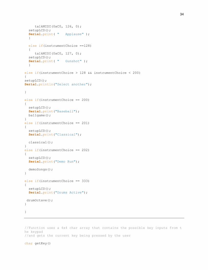
else if(instrumentChoice ==128)
talkMIDI(0xC0, 127, 0);
setupLCD();
Serial.print( " Gunshot" );
else if(instrumentChoice > 128 && instrumentChoice < 200)
setupLCD();
Serial.println("Select another");
else if(instrumentChoice == 200)
setupLCD();
Serial.print("Baseball");
ballgame();
else if(instrumentChoice == 201)
setupLCD();
Serial.print("Classical");
classical();
else if(instrumentChoice == 202)
setupLCD();
Serial.print("Demo Run");
demoSongs();
else if(instrumentChoice == 333)
setupLCD();
Serial.print("Drums Active");
drumOctave();
//Function uses a 4x4 char array that contains the possible key inputs from t
he keypad
//and gets the current key being pressed by the user
char getKey()

35
char key = 0; // 0 indicates no key pressed
for(int column = 0; column < numCols; column++)
digitalWrite(colPins[column],LOW); // Activate the current
column.
for(int row = 0; row < numRows; row++) // Scan all rows for
// a key press.
if(digitalRead(rowPins[row]) == LOW) // Is a key pressed?
delay(debounceTime); // debounce
while(digitalRead(rowPins[row]) == LOW)
; // wait for key to be released
key = keymap[row][column]; // Remember which key
// was pressed.
digitalWrite(colPins[column],HIGH); // De-activate the current
column.
return key; // returns the key pressed or 0 if none
//Conbines the imputs from the keypad into a 1,2, or 3 digit number
int threeDigits()
char ENTER_KEY = '#'; // if the # key is pressed, the loop breaks and the
user is finished entering the number
int val = 0;
int valKeys = 0;
for (;;) // Infinite foor loop to listen for key presses
char buttons;
buttons = getKey(); // use getKey() function to get the current key
if ((buttons >= '0') && (buttons <= '9')) // MAkes sure user enters valid
numbers from 0 to 9
// add the key's value to the accumulator
val = (val * 10) + (buttons - '0');
valKeys++;
else if (buttons == ENTER_KEY) // If user presses #, break from the
infinite loop and return the value they entered
break;
return(val);
36
//Makes the keyboard come alive, hasa foor loop that is checking to see what
sensor is pressed. Depending on the sensor
// the code plays the appropriate note on the octave scale and then tells the
7-segment display to display the appropraite
// number
void playOctave()
for (int thisSensor =0; thisSensor < 8; thisSensor++)
// get a sensor reading:
int sensorReading = analogRead(thisSensor);
// if the sensor is pressed hard enough:
if (sensorReading > threshold )
// Plays a middle C
if(thisSensor == 0)
writeMiddleC();
noteOn(0, 60, 60);
delay(50);
noteOff(0, 60, 60);
delay(50);
// Plays a D
else if(thisSensor == 1)
writeD();
noteOn(0, 62, 60);
delay(50);
noteOff(0, 62, 60);
delay(50);
// Plays a E
else if(thisSensor == 2)
writeE();
noteOn(0, 64, 60);
delay(50);
noteOff(0, 64, 60);
delay(50);
// Plays a F
else if(thisSensor == 3)

37
writeF();
noteOn(0, 65, 60);
delay(50);
noteOff(0, 65, 60);
delay(50);
// Plays a G
else if(thisSensor == 4)
writeG();
noteOn(0, 67, 60);
delay(50);
noteOff(0, 67, 60);
delay(50);
// Plays an A
else if(thisSensor == 5)
writeA();
noteOn(0, 69, 60);
delay(50);
noteOff(0, 69, 60);
delay(50);
// Plays a B
else if(thisSensor == 6)
writeB();
noteOn(0, 71, 60);
delay(50);
noteOff(0, 71, 60);
delay(50);
// Plays a C
else if(thisSensor ==7)
writeC();
noteOn(0, 72, 60);
delay(50);
noteOff(0, 72, 60);
delay(50) ;

38
void drumOctave()
talkMIDI(0xB0, 0, 0x78);
for (int drumSensor =8; drumSensor < 13; drumSensor++)
// get a sensor reading:
int sensReading = analogRead(drumSensor);
// if the sensor is pressed hard enough:
if (sensReading > threshold )
// Plays a middle C
if(drumSensor == 0)
// writeMiddleC();
// talkMIDI(0xC0, 27, 0);
noteOn(0, 35, 127);
delay(5);
noteOff(0, 35, 127);
delay(5);
// Plays a D
else if(drumSensor == 1)
// writeD();
// talkMIDI(0xC0, 35, 0);
noteOn(0, 36, 127);
delay(5);
noteOff(0, 36, 127);
delay(5);
// Plays a E
else if(drumSensor == 2)
// writeE();
// talkMIDI(0xC0, 35, 0);
noteOn(0, 39, 127);
delay(5);
noteOff(0, 39, 127);
delay(5);
// Plays a F
else if(drumSensor == 3)
// writeF();
// talkMIDI(0xC0, 40, 0);
noteOn(0, 50, 127);
delay(5);
noteOff(0, 50, 127);

39
delay(5);
// Plays a G
else if(drumSensor == 4)
// writeG();
// talkMIDI(0xC0, 49, 0);
noteOn(0, 56, 127);
delay(5);
noteOff(0, 56, 127);
delay(5);
// Plays an A
else if(drumSensor == 5)
// writeA();
// talkMIDI(0xC0, 54, 0);
noteOn(0, 58, 127);
delay(5);
noteOff(0, 58, 127);
delay(5);
// Plays a B
else if(drumSensor == 6)
// writeB();
// talkMIDI(0xC0, 77, 0);
noteOn(0, 60, 127);
delay(5);
noteOff(0, 60, 127);
delay(5);
// Plays a C
else if(drumSensor ==7)
// writeC();
// talkMIDI(0xC0, 70, 0);
noteOn(0, 72, 127);
delay(5);
noteOff(0, 72, 127);
delay(5);
void ballgame()
//Plays take me out to the ballgame with the instrument that the user current
ly has selected

40
//Code cycles thru appropriate notes for the song, turning on and off when ne
cessary
noteOn(0, 60, 60); // Turns note on
delay(250); // Parameter is in milliseconds, the delay function is
called throughout this function with a different
// time depending on the point in the song so that the
beat is as close as possible to the actual one
noteOff(0, 60, 60); // Turns note off
delay(250);
noteOn(0, 72, 60);
delay(250);
noteOff(0, 72, 60);
delay(150);
noteOn(0, 69, 60);
delay(200);
noteOff(0, 69, 60);
delay(200);
noteOn(0, 67, 60);
delay(250);
noteOff(0, 67, 60);
delay(250);
noteOn(0, 64, 60);
delay(250);
noteOff(0, 64, 60);
delay(250);
noteOn(0, 67, 60);
delay(350);
noteOff(0, 67, 60);
delay(350);
noteOn(0, 62, 60);
delay(250);
noteOff(0, 62, 60);
delay(250);
noteOn(0, 60, 60);
delay(250);
noteOff(0, 60, 60);
delay(250);
noteOn(0, 72, 60);
delay(250);
noteOff(0, 72, 60);
delay(150);
noteOn(0, 69, 60);
delay(200);
noteOff(0, 69, 60);
delay(200);

41
noteOn(0, 67, 60);
delay(250);
noteOff(0, 67, 60);
delay(250);
noteOn(0, 64, 60);
delay(250);
noteOff(0, 64, 60);
delay(250);
noteOn(0, 67, 60);
delay(350);
noteOff(0, 67, 60);
delay(350);
void classical() // Plays a classical piece
//Plays a classical song instrument that the user currently has selected
//Code cycles thru appropriate notes for the song, turning on and off when ne
cessary
noteOn(0, 64, 60);// Turns note on
delay(250); // Parameter is in milliseconds, the delay function is
called throughout this function with a different
// time depending on the point in the song so that the
beat is as close as possible to the actual one
noteOff(0, 64, 60);// Turns note off
delay(250);
noteOn(0, 64, 60);
delay(250);
noteOff(0, 64, 60);
delay(250);
noteOn(0, 65, 60);
delay(250);
noteOff(0, 65, 60);
delay(250);
noteOn(0, 67, 60);
delay(250);
noteOff(0, 67, 60);
delay(250);
noteOn(0, 67, 60);
delay(250);
noteOff(0, 67, 60);
delay(250);

42
noteOn(0, 65, 60);
delay(250);
noteOff(0, 65, 60);
delay(250);
noteOn(0, 64, 60);
delay(250);
noteOff(0, 64, 60);
delay(250);
noteOn(0, 62, 60);
delay(250);
noteOff(0, 62, 60);
delay(250);
noteOn(0, 60, 60);
delay(250);
noteOff(0, 60, 60);
delay(250);
noteOn(0, 60, 60);
delay(250);
noteOff(0, 60, 60);
delay(250);
noteOn(0, 62, 60);
delay(250);
noteOff(0, 62, 60);
delay(250);
noteOn(0, 64, 60);
delay(250);
noteOff(0, 64, 60);
delay(250);
noteOn(0, 64, 60);
delay(250);
noteOff(0, 64, 60);
delay(250);
noteOn(0, 62, 60);
delay(150);
noteOff(0, 62, 60);
delay(150);
noteOn(0, 62, 60);
delay(150);
noteOff(0, 62, 60);
delay(150);
void demoSongs()

43
talkMIDI(0xB0, 0x07, 120); //0xB0 is channel message, set channel volume to
near max (127)
Serial.println("Basic Instruments");
talkMIDI(0xB0, 0, 0x00); //Default bank GM1
//Change to different instrument
for(instrument = 0 ; instrument < 127 ; instrument++)
Serial.print(" Instrument: ");
Serial.println(instrument, DEC);
// Tell board what instrument you want
talkMIDI(0xC0, instrument, 0); //Set instrument number. 0xC0 is a 1 data
byte command
//Cycles through a scale
//Note on channel 1 (0x90), some note value (note), middle velocity
(0x45):
//Note controls the tone of the instrument, test this against tuner
// thrid param controls force it is play at, higher number means louder
for (int thisSensor =6; thisSensor < 10; thisSensor++)
// get a sensor reading:
int sensorReading = analogRead(thisSensor);
// if the sensor is pressed hard enough:
if (sensorReading > threshold)
if(thisSensor == 6)
noteOn(0, 50, 60);
delay(50);
else if (thisSensor ==7)
noteOn(0, 52, 60);
delay(50);
else if (thisSensor ==8)
noteOn(0, 54, 60);
delay(50);
else if (thisSensor ==9)
noteOn(0, 56, 60);
delay(50);
44
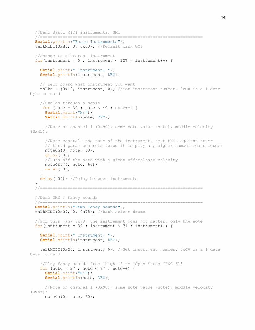
//Demo Basic MIDI instruments, GM1
//=================================================================
Serial.println("Basic Instruments");
talkMIDI(0xB0, 0, 0x00); //Default bank GM1
//Change to different instrument
for(instrument = 0 ; instrument < 127 ; instrument++)
Serial.print(" Instrument: ");
Serial.println(instrument, DEC);
// Tell board what instrument you want
talkMIDI(0xC0, instrument, 0); //Set instrument number. 0xC0 is a 1 data
byte command
//Cycles through a scale
for (note = 30 ; note < 40 ; note++)
Serial.print("N:");
Serial.println(note, DEC);
//Note on channel 1 (0x90), some note value (note), middle velocity
(0x45):
//Note controls the tone of the instrument, test this against tuner
// thrid param controls force it is play at, higher number means louder
noteOn(0, note, 60);
delay(50);
//Turn off the note with a given off/release velocity
noteOff(0, note, 60);
delay(50);
delay(100); //Delay between instruments
//=================================================================
//Demo GM2 / Fancy sounds
//=================================================================
Serial.println("Demo Fancy Sounds");
talkMIDI(0xB0, 0, 0x78); //Bank select drums
//For this bank 0x78, the instrument does not matter, only the note
for(instrument = 30 ; instrument < 31 ; instrument++)
Serial.print(" Instrument: ");
Serial.println(instrument, DEC);
talkMIDI(0xC0, instrument, 0); //Set instrument number. 0xC0 is a 1 data
byte command
//Play fancy sounds from 'High Q' to 'Open Surdo [EXC 6]'
for (note = 27 ; note < 87 ; note++)
Serial.print("N:");
Serial.println(note, DEC);
//Note on channel 1 (0x90), some note value (note), middle velocity
(0x45):
noteOn(0, note, 60);
45
delay(100);
//Turn off the note with a given off/release velocity
noteOff(0, note, 60);
delay(100);
delay(100); //Delay between instruments
/*
//Demo Melodic
//=================================================================
Serial.println("Demo Melodic? Sounds");
talkMIDI(0xB0, 0, 0x79); //Bank select Melodic
//These don't sound different from the main bank to me
//Change to different instrument
for(instrument = 27 ; instrument < 87 ; instrument++)
Serial.print(" Instrument: ");
Serial.println(instrument, DEC);
talkMIDI(0xC0, instrument, 0); //Set instrument number. 0xC0 is a 1 data
byte command
//Play notes from F#-0 (30) to F#-5 (90):
for (note = 30 ; note < 40 ; note++)
Serial.print("N:");
Serial.println(note, DEC);
//Note on channel 1 (0x90), some note value (note), middle velocity (0x
45):
noteOn(0, note, 60);
delay(50);
//Turn off the note with a given off/release velocity
noteOff(0, note, 60);
delay(50);
delay(100); //Delay between instruments
*/
//Send a MIDI note-on message. Like pressing a piano key
//channel ranges from 0-15
#include <Servo.h>

46
Servo myservo; // create servo object to control a servo
// a maximum of eight servo objects can be created
int pos = 0; // variable to store the servo position
int servoPin = 2;
void setup()
Serial.begin(9600);
myservo.attach(3);
pinMode(servoPin ,INPUT);
void loop()
int buttonState = digitalRead(servoPin);
Serial.println(buttonState);
if (buttonState == 1)
callServo();
// waits 15ms for the servo to reach the position
void callServo()
for(pos = 0; pos < 180; pos += 90) // goes from 0 degrees to 180 degrees
// in steps of 1 degree
myservo.write(pos);
// tell servo to go to position in variable 'pos'
delay(120) ; // waits 15ms for the servo to reach the
position
for(pos = 180; pos > 0; pos -= 90 ) // goes from 0 degrees to
180 degrees
// in steps of 1 degree
myservo.write(pos); // tell servo to go to position in
variable 'pos'
delay(120) ; // waits 15ms for the servo to reach the
position;
Appendix B: References o Musical Instrument Shield Quick Start Guide
o https://www.sparkfun.com/tutorials/302
o Arduino Keypad Tutorial
o http://playground.arduino.cc/Main/KeypadTutorial
o How a Keypad Works
o http://www.youtube.com/watch?v=gWvIzQLoP0I

47
Appendix C: Spec Sheets

TDSG5150, TDSG5160, TDSO5150, TDSO5160, TDSY5150, TDSY5160www.vishay.com Vishay Semiconductors
Rev. 1.7, 17-Apr-13 1 Document Number: 83126
For technical questions, contact: [email protected] DOCUMENT IS SUBJECT TO CHANGE WITHOUT NOTICE. THE PRODUCTS DESCRIBED HEREIN AND THIS DOCUMENT
ARE SUBJECT TO SPECIFIC DISCLAIMERS, SET FORTH AT www.vishay.com/doc?91000
Standard 7-Segment Display 13 mm
DESCRIPTIONThe TDS.51.. series are 13 mm character seven segment LED displays in a very compact package.
The displays are designed for a viewing distance up to 7 m and available in four bright colors. The grey package surface and the evenly lighted untinted segments provide an optimum on-off contrast.
All displays are categorized in luminous intensity groups. That allows users to assemble displays with uniform appearence. Typical applications include instruments, panel meters, point-of-sale terminals and household equipment.
FEATURES• Evenly lighted segments
• Grey package surface
• Untinted segments
• Luminous intensity categorized
• Yellow and green categorized for color
• Wide viewing angle
• Suitable for DC and high peak current
• Material categorization: For definitions of compliance please see www.vishay.com/doc?99912
APPLICATIONS• Panel meters
• Test- and measure-equipment
• Point-of-sale terminals
• Control units
• TV sets
PRODUCT GROUP AND PACKAGE DATA• Product group: Display
• Package: 13 mm
• Product series: Standard
• Angle of half intensity: ± 50°
19237
PARTS TABLE
PART COLORLUMINOUS INTENSITY
(μcd)atIF
(mA)
WAVELENGTH(nm)
atIF
(mA)
FORWARD VOLTAGE(V)
atIF
(mA)CIRCUITRY
MIN. TYP. MAX. MIN. TYP. MAX. MIN. TYP. MAX.
TDSO5150 Orange red 700 5000 - 10 612 - 625 10 - 2 3 20 Common anode
TDSO5150-LM Orange red 2800 - 9000 10 612 - 625 10 - 2 3 20 Common anode
TDSO5150-M Orange red 4500 - 9000 10 612 - 625 10 - 2 3 20 Common anode
TDSO5160 Orange red 700 5000 - 10 612 - 625 10 - 2 3 20 Common cathode
TDSO5160-LM Orange red 2800 - 9000 10 612 - 625 10 - 2 3 20 Common cathode
TDSY5150 Yellow 700 4200 - 10 581 - 594 10 - 2.4 3 20 Common anode
TDSY5160 Yellow 700 4200 - 10 581 - 594 10 - 2.4 3 20 Common cathode
TDSG5150 Green 700 9500 - 10 562 - 575 10 - 2.4 3 20 Common anode
TDSG5150-MN Green 4500 - 14 000 10 562 - 575 10 - 2.4 3 20 Common anode
TDSG5150-N Green 7000 - 14 000 10 562 - 575 10 - 2.4 3 20 Common anode
TDSG5160 Green 700 9500 - 10 562 - 575 10 - 2.4 3 20 Common cathode
TDSG5160-MN Green 4500 - 14 000 10 562 - 575 10 - 2.4 3 20 Common cathode
TDSG5160-N Green 7000 - 14 000 10 562 - 575 10 - 2.4 3 20 Common cathode

TDSG5150, TDSG5160, TDSO5150, TDSO5160, TDSY5150, TDSY5160www.vishay.com Vishay Semiconductors
Rev. 1.7, 17-Apr-13 2 Document Number: 83126
For technical questions, contact: [email protected] DOCUMENT IS SUBJECT TO CHANGE WITHOUT NOTICE. THE PRODUCTS DESCRIBED HEREIN AND THIS DOCUMENT
ARE SUBJECT TO SPECIFIC DISCLAIMERS, SET FORTH AT www.vishay.com/doc?91000
Note(1) IVmin. and IV groups are mean values of all segments (a to g, D1 to D4), matching factor within segments is 0.5, excluding decimal points
and colon.
Note(1) IVmin. and IV groups are mean values of all segments (a to g, D1 to D4), matching factor within segments is 0.5, excluding decimal points
and colon.
ABSOLUTE MAXIMUM RATINGS (Tamb = 25 °C, unless otherwise specified)TDSO5150, TDSO5160, TDSY5150, TDSY5160, TDSG5150, TDSG5160PARAMETER TEST CONDITION SYMBOL VALUE UNIT
Reverse voltage per segment or DP VR 6 V
DC forward current per segment or DP IF 25 mA
Surge forward current per segment or DP tp 10 μs (non repetitive) IFSM 0.15 A
Power dissipation Tamb 45 °C PV 550 mW
Junction temperature Tj 100 °C
Operating temperature range Tamb - 40 to + 85 °C
Storage temperature range Tstg - 40 to + 85 °C
Soldering temperature t 3 s, 2 mm below seating plane Tsd 260 °C
Thermal resistance LED junction/ambient RthJA 100 K/W
OPTICAL AND ELECTRICAL CHARACTERISTICS (Tamb = 25 °C, unless otherwise specified)TDSO5150, TDSO5150-LM, TDSO5150-M, TDSO5160, TDSO5160-LM, ORANGE REDPARAMETER TEST CONDITION PART SYMBOL MIN. TYP. MAX. UNIT
Luminous intensity per segment(digit average) (1) IF = 10 mA
TDSO5150
IV
700 5000 -
μcd
TDSO5150-LM 2800 - 9000
TDSO5150-M 4500 - 9000
TDSO5160 700 5000 -
TDSO5160-LM 2800 - 9000
Dominant wavelength IF = 10 mATDSO5150,
TDSO5150-LM, TDSO5150-M,
TDSO5160, TDSO5160-LM
d 612 - 625 nm
Peak wavelength IF = 10 mA p - 630 - nm
Angle of half intensity IF = 10 mA j - ± 50 - deg
Forward voltage per segment or DP IF = 20 mA VF - 2 3 V
Reverse voltage per segment or DP IR = 10 μA VR 6 15 - V
OPTICAL AND ELECTRICAL CHARACTERISTICS (Tamb = 25 °C, unless otherwise specified)TDSY5150, TDSY5160, YELLOWPARAMETER TEST CONDITION PART SYMBOL MIN. TYP. MAX. UNIT
Luminous intensity per segment(digit average) (1) IF = 10 mA
TDSY5150IV
700 4200 -μcd
TDSY5160 700 4200 -
Dominant wavelength IF = 10 mA
TDSY5150,TDSY5160
d 581 - 594 nm
Peak wavelength IF = 10 mA p - 585 - nm
Angle of half intensity IF = 10 mA j - ± 50 - deg
Forward voltage per segment or DP IF = 20 mA VF - 2.4 3 V
Reverse voltage per segment or DP IR = 10 μA VR 6 15 - V

TDSG5150, TDSG5160, TDSO5150, TDSO5160, TDSY5150, TDSY5160www.vishay.com Vishay Semiconductors
Rev. 1.7, 17-Apr-13 3 Document Number: 83126
For technical questions, contact: [email protected] DOCUMENT IS SUBJECT TO CHANGE WITHOUT NOTICE. THE PRODUCTS DESCRIBED HEREIN AND THIS DOCUMENT
ARE SUBJECT TO SPECIFIC DISCLAIMERS, SET FORTH AT www.vishay.com/doc?91000
Note(1) IVmin. and IV groups are mean values of all segments (a to g, D1 to D4), matching factor within segments is 0.5, excluding decimal points
and colon.
Note• The above type numbers represent the order groups which
include only a few brightness groups. Only one group will be shipped in one tube (there will be no mixing of two groups in one tube).In order to ensure availability, single brightness groups will not be orderable.
Note• Wavelengths are tested at a current pulse duration of 25 ms and
an accuracy of ± 1 nm.
OPTICAL AND ELECTRICAL CHARACTERISTICS (Tamb = 25 °C, unless otherwise specified)TDSG5150, TDSG5150-MN, TDSG5150-N, TDSG5160, TDSG5160-MN, TDSG5160-N, GREENPARAMETER TEST CONDITION PART SYMBOL MIN. TYP. MAX. UNIT
Luminous intensity per segment(digit average) (1) IF = 10 mA
TDSG5150
IV
700 9500 -
μcd
TDSG5150-MN 4500 - 14 000
TDSG5150-N 7000 - 14 000
TDSG5160 700 9500 -
TDSG5160-MN 4500 - 14 000
TDSG5160-N 7000 - 14 000
Dominant wavelength IF = 10 mA TDSG5150, TDSG5150-MN, TDSG5150-N.
TDSG5160, TDSG5160-MN,
TDSG5160-N
d 562 - 575 nm
Peak wavelength IF = 10 mA p - 565 - nm
Angle of half intensity IF = 10 mA j - ± 50 - deg
Forward voltage per segment or DP IF = 20 mA VF - 2.4 3 V
Reverse voltage per segment or DP IR = 10 μA VR 6 15 - V
LUMINOUS INTENSITY CLASSIFICATIONGROUP LIGHT INTENSITY (μcd)
STANDARD MIN. MAX.
E 180 360
F 280 560
G 450 900
H 700 1400
I 1100 2200
K 1800 3600
L 2800 5600
M 4500 9000
N 7000 14 000
COLOR CLASSIFICATION
GROUPORANGE RED YELLOW GREEN
MIN. MAX. MIN. MAX. MIN. MAX.
1 598 601 581 584
2 600 603 583 586 562 565
3 602 605 585 588 564 567
4 604 607 587 590 566 569
5 606 609 589 592 568 571
6 608 611 591 594 570 573
7 570 575

TDSG5150, TDSG5160, TDSO5150, TDSO5160, TDSY5150, TDSY5160www.vishay.com Vishay Semiconductors
Rev. 1.7, 17-Apr-13 4 Document Number: 83126
For technical questions, contact: [email protected] DOCUMENT IS SUBJECT TO CHANGE WITHOUT NOTICE. THE PRODUCTS DESCRIBED HEREIN AND THIS DOCUMENT
ARE SUBJECT TO SPECIFIC DISCLAIMERS, SET FORTH AT www.vishay.com/doc?91000
TYPICAL CHARACTERISTICS (Tamb = 25 °C, unless otherwise specified)
Fig. 1 - Forward Current vs. Ambient Temperature
Fig. 2 - Relative Luminous Intensity vs. Angular Displacement
Fig. 3 - Forward Current vs. Forward Voltage
Fig. 4 - Relative Luminous Intensity vs. Ambient Temperature
Fig. 5 - Relative Luminous Intensity vs. Forward Current/Duty Cycle
Fig. 6 - Relative Luminous Intensity vs. Forward Current
0
10
20
30
40
60
0 20 40 60 80
I-
For
war
d C
urre
nt (
mA
)F
Tamb - Ambient Temperature (°C)
100
17525
50
0.4 0.2 0
95 10082
0.6
0.9
0.8
0°30°
10° 20°
40°
50°
60°
70°
80°0.7
1.0
I V r
el -
Rel
ativ
e Lu
min
ous
Inte
nsity
ϕ -
Ang
ular
Dis
plac
emen
t
I-
For
war
dC
urre
nt (
mA
)F
0.1
1
10
100
1000
18794 VF - Forward Voltage (V)
Orange Red
tp /T = 0.001tp = 10 µs
1086420
0.0
0.2
0.4
0.6
0.8
1.0
1.2
1.4
1.6
0 10 20 30 40 50 60 70 80 90 100
Tamb - Ambient Temperature (°C)18795
Orange Red
IF = 10 mA
I-
Rel
ativ
eLu
min
ous
Inte
nsity
Vre
l
10 20 50 100 2000
0.4
0.8
1.2
1.6
2.4
18796
500
0.5 0.2 0.1 0.05 0.021
IF(mA)
tp/T
2.0Orange Red
IFAV = 10 mA, const.I-
Spe
cific
Lum
inou
sIn
tens
ityV
rel
1 100.01
0.1
1
10
IF - Forward Current (mA)
100
18797
Orange Red
I-
Rel
ativ
eLu
min
ous
Inte
nsity
Vre
l

TDSG5150, TDSG5160, TDSO5150, TDSO5160, TDSY5150, TDSY5160www.vishay.com Vishay Semiconductors
Rev. 1.7, 17-Apr-13 5 Document Number: 83126
For technical questions, contact: [email protected] DOCUMENT IS SUBJECT TO CHANGE WITHOUT NOTICE. THE PRODUCTS DESCRIBED HEREIN AND THIS DOCUMENT
ARE SUBJECT TO SPECIFIC DISCLAIMERS, SET FORTH AT www.vishay.com/doc?91000
Fig. 7 - Relative Intensity vs. Wavelength
Fig. 8 - Forward Current vs. Forward Voltage
Fig. 9 - Relative Luminous Intensity vs. Ambient Temperature
Fig. 10 - Relative Luminous Intensity vs.Forward Current/Duty Cycle
Fig. 11 - Relative Luminous Intensity vs. Forward Current
Fig. 12 - Relative Intensity vs. Wavelength
590 610 630 650 6700
0.2
0.4
0.6
0.8
1.2
690
17529 λ - Wavelength (nm)
1.0Orange Red
I-
Rel
ativ
eIn
tens
ityre
l
0.1
1
10
100
1000
1086420
95 10030 VF - Forward Voltage (V)
I F -
For
war
d C
urre
nt (
mA
) yellow
tp/T = 0.001tp = 10 µs
00
0.4
0.8
1.2
1.6
95 10031
20 40 60 80 100
I V r
el -
Rel
ativ
e Lu
min
ous
Inte
nsity
Tamb - Ambient Temperature (°C)
yellow
IF = 10 mA
yellow
10 20 50 100 2000
0.4
0.8
1.2
1.6
2.4
95 10260
500
0.5 0.2 0.1 0.05 0.021
IF (mA)
tp/T
I spe
c -
Spe
cific
Lum
inou
s In
tens
ity
2.0
yellow
IF - Forward Current (mA)100
0.1
1
10
95 10033
I V r
el -
Rel
ativ
e Lu
min
ous
Inte
nsity
1010.01
550 570 590 610 6300
0.2
0.4
0.6
0.8
1.2
650
95 10039 λ - Wavelength (nm)
1.0yellow
I rel -
Rel
ativ
e In
tens
ity
TDSG5150, TDSG5160, TDSO5150, TDSO5160, TDSY5150, TDSY5160www.vishay.com Vishay Semiconductors
Rev. 1.7, 17-Apr-13 6 Document Number: 83126
For technical questions, contact: [email protected] DOCUMENT IS SUBJECT TO CHANGE WITHOUT NOTICE. THE PRODUCTS DESCRIBED HEREIN AND THIS DOCUMENT
ARE SUBJECT TO SPECIFIC DISCLAIMERS, SET FORTH AT www.vishay.com/doc?91000
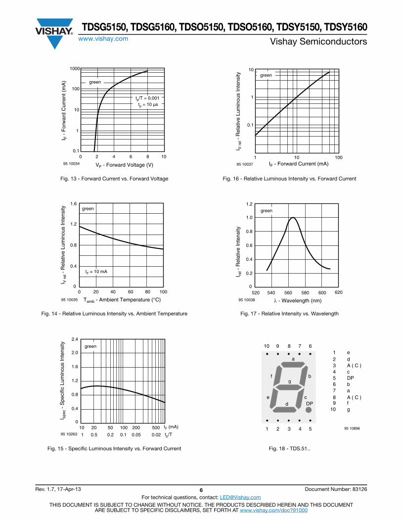
Fig. 13 - Forward Current vs. Forward Voltage
Fig. 14 - Relative Luminous Intensity vs. Ambient Temperature
Fig. 15 - Specific Luminous Intensity vs. Forward Current
Fig. 16 - Relative Luminous Intensity vs. Forward Current
Fig. 17 - Relative Intensity vs. Wavelength
Fig. 18 - TDS.51..
0.1
1
10
100
1000
1086420
95 10034 VF - Forward Voltage (V)
I F -
For
war
d C
urre
nt (
mA
) green
tp/T = 0.001tp = 10 µs
0
0.4
0.8
1.2
1.6
95 10035
I V r
el -
Rel
ativ
e Lu
min
ous
Inte
nsity green
IF = 10 mA
Tamb - Ambient Temperature (°C)
20 40 60 800 100
10 20 50 100 2000
0.4
0.8
1.2
1.6
2.4
95 10263
500
2.0green
I spe
c -
Spe
cific
Lum
inou
s In
tens
ity
IF (mA)
0.5 0.2 0.1 0.05 0.021 tp/T
IF - Forward Current (mA)100
green
0.1
1
10
95 10037
I V r
el -
Rel
ativ
e Lu
min
ous
Inte
nsity
101
520 540 560 580 6000
0.2
0.4
0.6
0.8
1.2
620
95 10038 λ - Wavelength (nm)
1.0
green
I rel -
Rel
ativ
e In
tens
ity
a
f
e
g
dc
b
DP
1 2 3 4 5
10 9 8 7 6
95 10896
1 e2 d
4 c
6 b
9 f10 g
7 a
5 DP
3 A ( C )
8 A ( C )

TDSG5150, TDSG5160, TDSO5150, TDSO5160, TDSY5150, TDSY5160www.vishay.com Vishay Semiconductors
Rev. 1.7, 17-Apr-13 7 Document Number: 83126
For technical questions, contact: [email protected] DOCUMENT IS SUBJECT TO CHANGE WITHOUT NOTICE. THE PRODUCTS DESCRIBED HEREIN AND THIS DOCUMENT
ARE SUBJECT TO SPECIFIC DISCLAIMERS, SET FORTH AT www.vishay.com/doc?91000
PACKAGE DIMENSIONS FOR TDS.51.. in millimeters
95 11344
Drawing-No.: 6.544-5150.01-4Issue: 1; 21.11.95

VISHAY Display-13 mm
Document Number 83927
Rev. 1.1, 25-Mar-04
Vishay Semiconductors
www.vishay.com
1
Display-13 mm
Package Dimensions in mm
95 11344

www.vishay.com
2
Document Number 83927
Rev. 1.1, 25-Mar-04
VISHAYDisplay-13 mmVishay Semiconductors
Ozone Depleting Substances Policy Statement
It is the policy of Vishay Semiconductor GmbH to
1. Meet all present and future national and international statutory requirements.
2. Regularly and continuously improve the performance of our products, processes, distribution and operatingsystems with respect to their impact on the health and safety of our employees and the public, as well as their impact on the environment.
It is particular concern to control or eliminate releases of those substances into the atmosphere which are known as ozone depleting substances (ODSs).
The Montreal Protocol (1987) and its London Amendments (1990) intend to severely restrict the use of ODSs and forbid their use within the next ten years. Various national and international initiatives are pressing for an earlier ban on these substances.
Vishay Semiconductor GmbH has been able to use its policy of continuous improvements to eliminate the use of ODSs listed in the following documents.
1. Annex A, B and list of transitional substances of the Montreal Protocol and the London Amendments respectively
2. Class I and II ozone depleting substances in the Clean Air Act Amendments of 1990 by the Environmental Protection Agency (EPA) in the USA
3. Council Decision 88/540/EEC and 91/690/EEC Annex A, B and C (transitional substances) respectively.
Vishay Semiconductor GmbH can certify that our semiconductors are not manufactured with ozone depleting substances and do not contain such substances.
We reserve the right to make changes to improve technical design and may do so without further notice.
Parameters can vary in different applications. All operating parameters must be validated for each customer application by the customer. Should the buyer use Vishay Semiconductors products for any unintended or unauthorized application, the buyer shall indemnify Vishay Semiconductors against all
claims, costs, damages, and expenses, arising out of, directly or indirectly, any claim of personal damage, injury or death associated with such unintended or unauthorized use.
Vishay Semiconductor GmbH, P.O.B. 3535, D-74025 Heilbronn, GermanyTelephone: 49 (0)7131 67 2831, Fax number: 49 (0)7131 67 2423

VISHAY Pin Connections 13 mm
Document Number 83994
Rev. 1.1, 07-Jul-04
Vishay Semiconductors
www.vishay.com
1
Pin Connections 13 mm
a
f
e
g
d
c
b
DP
1 2 3 4 5
10 9 8 7 6
95 10896
1 e
2 d
4 c
6 b
9 f
10 g
7 a
5 DP
3 A ( C )
8 A ( C )

www.vishay.com
2
Document Number 83994
Rev. 1.1, 07-Jul-04
VISHAYPin Connections 13 mmVishay Semiconductors
Ozone Depleting Substances Policy Statement
It is the policy of Vishay Semiconductor GmbH to
1. Meet all present and future national and international statutory requirements.
2. Regularly and continuously improve the performance of our products, processes, distribution and operatingsystems with respect to their impact on the health and safety of our employees and the public, as well as their impact on the environment.
It is particular concern to control or eliminate releases of those substances into the atmosphere which are known as ozone depleting substances (ODSs).
The Montreal Protocol (1987) and its London Amendments (1990) intend to severely restrict the use of ODSs and forbid their use within the next ten years. Various national and international initiatives are pressing for an earlier ban on these substances.
Vishay Semiconductor GmbH has been able to use its policy of continuous improvements to eliminate the use of ODSs listed in the following documents.
1. Annex A, B and list of transitional substances of the Montreal Protocol and the London Amendments respectively
2. Class I and II ozone depleting substances in the Clean Air Act Amendments of 1990 by the Environmental Protection Agency (EPA) in the USA
3. Council Decision 88/540/EEC and 91/690/EEC Annex A, B and C (transitional substances) respectively.
Vishay Semiconductor GmbH can certify that our semiconductors are not manufactured with ozone depleting substances and do not contain such substances.
We reserve the right to make changes to improve technical design and may do so without further notice.
Parameters can vary in different applications. All operating parameters must be validated for each customer application by the customer. Should the buyer use Vishay Semiconductors products for any unintended or unauthorized application, the buyer shall indemnify Vishay Semiconductors against all
claims, costs, damages, and expenses, arising out of, directly or indirectly, any claim of personal damage, injury or death associated with such unintended or unauthorized use.
Vishay Semiconductor GmbH, P.O.B. 3535, D-74025 Heilbronn, GermanyTelephone: 49 (0)7131 67 2831, Fax number: 49 (0)7131 67 2423

Legal Disclaimer Noticewww.vishay.com Vishay
Revision: 02-Oct-12 1 Document Number: 91000
DisclaimerALL PRODUCT, PRODUCT SPECIFICATIONS AND DATA ARE SUBJECT TO CHANGE WITHOUT NOTICE TO IMPROVERELIABILITY, FUNCTION OR DESIGN OR OTHERWISE.
Vishay Intertechnology, Inc., its affiliates, agents, and employees, and all persons acting on its or their behalf (collectively,“Vishay”), disclaim any and all liability for any errors, inaccuracies or incompleteness contained in any datasheet or in any otherdisclosure relating to any product.
Vishay makes no warranty, representation or guarantee regarding the suitability of the products for any particular purpose orthe continuing production of any product. To the maximum extent permitted by applicable law, Vishay disclaims (i) any and allliability arising out of the application or use of any product, (ii) any and all liability, including without limitation special,consequential or incidental damages, and (iii) any and all implied warranties, including warranties of fitness for particularpurpose, non-infringement and merchantability.
Statements regarding the suitability of products for certain types of applications are based on Vishay’s knowledge of typicalrequirements that are often placed on Vishay products in generic applications. Such statements are not binding statementsabout the suitability of products for a particular application. It is the customer’s responsibility to validate that a particularproduct with the properties described in the product specification is suitable for use in a particular application. Parametersprovided in datasheets and/or specifications may vary in different applications and performance may vary over time. Alloperating parameters, including typical parameters, must be validated for each customer application by the customer’stechnical experts. Product specifications do not expand or otherwise modify Vishay’s terms and conditions of purchase,including but not limited to the warranty expressed therein.
Except as expressly indicated in writing, Vishay products are not designed for use in medical, life-saving, or life-sustainingapplications or for any other application in which the failure of the Vishay product could result in personal injury or death.Customers using or selling Vishay products not expressly indicated for use in such applications do so at their own risk. Pleasecontact authorized Vishay personnel to obtain written terms and conditions regarding products designed for such applications.
No license, express or implied, by estoppel or otherwise, to any intellectual property rights is granted by this document or byany conduct of Vishay. Product names and markings noted herein may be trademarks of their respective owners.
Material Category PolicyVishay Intertechnology, Inc. hereby certifies that all its products that are identified as RoHS-Compliant fulfill thedefinitions and restrictions defined under Directive 2011/65/EU of The European Parliament and of the Councilof June 8, 2011 on the restriction of the use of certain hazardous substances in electrical and electronic equipment(EEE) - recast, unless otherwise specified as non-compliant.
Please note that some Vishay documentation may still make reference to RoHS Directive 2002/95/EC. We confirm thatall the products identified as being compliant to Directive 2002/95/EC conform to Directive 2011/65/EU.
Vishay Intertechnology, Inc. hereby certifies that all its products that are identified as Halogen-Free follow Halogen-Freerequirements as per JEDEC JS709A standards. Please note that some Vishay documentation may still make referenceto the IEC 61249-2-21 definition. We confirm that all the products identified as being compliant to IEC 61249-2-21conform to JEDEC JS709A standards.

Date Rev. Description
GOLDSUN ELECTRONICS CO., LTD.
UNIT: SCALE: CAS No:ERN No:SHEET 1 OF 1
DCC. NO.
A4 DRAWING NO.mm
Rev.Description1
DRAWN:
MATERIAL
Ivan Wang
VERIFY PEOPLE:
169245JAMECO NO. GOLDSUN NO.
TELEPHONE 4x4 KEYPADSBLACK COLORPenny
AK-1607-N-BBW

VLSISolution y VS1053b
VS1053B
VS1053b -Ogg Vorbis/MP3/AAC/WMA/MIDI
AUDIO CODECFeatures
• Decodes Ogg Vorbis;MPEG 1 & 2 audio layer III (CBR +VBR+ABR); layers I & II optional;MPEG4 / 2 AAC-LC(+PNS),HE-AAC v2 (Level 3) (SBR + PS);WMA 4.0/4.1/7/8/9 all profiles (5-384 kbps);WAV (PCM + IMA ADPCM);General MIDI 1 / SP-MIDI format 0 files
• Encodes Ogg Vorbis with software plu-gin (available Q4/2007)
• Encodes IMA ADPCM from mic/line (stereo)• Streaming support for MP3 and WAV• EarSpeaker Spatial Processing• Bass and treble controls• Operates with a single 12..13 MHz clock• Can also be used with a 24..26 MHz clock• Internal PLL clock multiplier• Low-power operation• High-quality on-chip stereo DAC with no
phase error between channels• Zero-cross detection for smooth volume
change• Stereo earphone driver capable of driving a
30 Ω load• Quiet power-on and power-off• I2S interface for external DAC• Separate voltages for analog, digital, I/O• On-chip RAM for user code and data• Serial control and data interfaces• Can be used as a slave co-processor• SPI flash boot for special applications• UART for debugging purposes• New functions may be added with software
and upto 8 GPIO pins• Lead-free RoHS-compliant package (Green)
Description
VS1053b is a single-chip Ogg Vorbis/MP3/AAC/-WMA/MIDI audio decoder and an IMA ADPCMand user-loadable Ogg Vorbis encoder. It containsa high-performance, proprietary low-power DSPprocessor core VS DSP4, working data memory,16 KiB instruction RAM and 0.5+ KiB data RAMfor user applications running simultaneously withany built-in decoder, serial control and input datainterfaces, upto 8 general purpose I/O pins, anUART, as well as a high-quality variable-sample-rate stereo ADC (mic, line, line + mic or 2×line)and stereo DAC, followed by an earphone ampli-fier and a common voltage buffer.
VS1053b receives its input bitstream through aserial input bus, which it listens to as a systemslave. The input stream is decoded and passedthrough a digital volume control to an 18-bit over-sampling, multi-bit, sigma-delta DAC. The decod-ing is controlled via a serial control bus. In addi-tion to the basic decoding, it is possible to addapplication specific features, like DSP effects, tothe user RAM memory.
Optional factory-programmable unique chip ID pro-vides basis for digital rights management or unitidentification features.
Instruction RAM
Instruction ROM
Stereo DAC
L
R
UART
SerialData/ControlInterface
Stereo Ear−phone Driver
DREQ
SO
SI
SCLK
XCS
RX
TX
audio
output
X ROM
X RAM
Y ROM
Y RAM
GPIOGPIO
VSDSP4
XDCS
MIC AMP
Clockmultiplier
MUX
8
I2S
VS1053StereoADC
differentialmic / line 1
line 2
Version 1.01, 2008-05-22 1
VLSISolution y VS1053b
VS1053B
CONTENTS
Contents
1 Licenses 9
2 Disclaimer 9
3 Definitions 9
4 Characteristics & Specifications 10
4.1 Absolute Maximum Ratings . . . . . . . . . . . . . . . . . . . . . . . . . . . . . . . . 10
4.2 Recommended Operating Conditions . . . . . . . . . . . . . . . . . . . . . . . . . . . . 10
4.3 Analog Characteristics . . . . . . . . . . . . . . . . . . . . . . . . . . . . . . . . . . . 11
4.4 Power Consumption . . . . . . . . . . . . . . . . . . . . . . . . . . . . . . . . . . . . . 12
4.5 Digital Characteristics . . . . . . . . . . . . . . . . . . . . . . . . . . . . . . . . . . . 12
4.6 Switching Characteristics - Boot Initialization . . . . . . . . . . . . . . . . . . . . . . . 12
5 Packages and Pin Descriptions 13
5.1 Packages . . . . . . . . . . . . . . . . . . . . . . . . . . . . . . . . . . . . . . . . . . 13
5.1.1 LQFP-48 . . . . . . . . . . . . . . . . . . . . . . . . . . . . . . . . . . . . . . 13
6 Connection Diagram, LQFP-48 16
7 SPI Buses 18
7.1 General . . . . . . . . . . . . . . . . . . . . . . . . . . . . . . . . . . . . . . . . . . . 18
7.2 SPI Bus Pin Descriptions . . . . . . . . . . . . . . . . . . . . . . . . . . . . . . . . . . 18
7.2.1 VS1002 Native Modes (New Mode) . . . . . . . . . . . . . . . . . . . . . . . . 18
7.2.2 VS1001 Compatibility Mode (deprecated) . . . . . . . . . . . . . . . . . . . . . 18
7.3 Data Request Pin DREQ . . . . . . . . . . . . . . . . . . . . . . . . . . . . . . . . . . 19
Version 1.01, 2008-05-22 2
VLSISolution y VS1053b
VS1053B
CONTENTS
7.4 Serial Protocol for Serial Data Interface (SDI) . . . . . . . . . . . . . . . . . . . . . . . 19
7.4.1 General . . . . . . . . . . . . . . . . . . . . . . . . . . . . . . . . . . . . . . . 19
7.4.2 SDI in VS1002 Native Modes (New Mode) . . . . . . . . . . . . . . . . . . . . 19
7.4.3 SDI in VS1001 Compatibility Mode (deprecated) . . . . . . . . . . . . . . . . . 20
7.4.4 Passive SDI Mode . . . . . . . . . . . . . . . . . . . . . . . . . . . . . . . . . 20
7.5 Serial Protocol for Serial Command Interface (SCI) . . . . . . . . . . . . . . . . . . . . 20
7.5.1 General . . . . . . . . . . . . . . . . . . . . . . . . . . . . . . . . . . . . . . . 20
7.5.2 SCI Read . . . . . . . . . . . . . . . . . . . . . . . . . . . . . . . . . . . . . . 21
7.5.3 SCI Write . . . . . . . . . . . . . . . . . . . . . . . . . . . . . . . . . . . . . . 21
7.5.4 SCI Multiple Write . . . . . . . . . . . . . . . . . . . . . . . . . . . . . . . . . 22
7.6 SPI Timing Diagram . . . . . . . . . . . . . . . . . . . . . . . . . . . . . . . . . . . . 23
7.7 SPI Examples with SM SDINEW and SM SDISHARED set . . . . . . . . . . . . . . . 24
7.7.1 Two SCI Writes . . . . . . . . . . . . . . . . . . . . . . . . . . . . . . . . . . . 24
7.7.2 Two SDI Bytes . . . . . . . . . . . . . . . . . . . . . . . . . . . . . . . . . . . 24
7.7.3 SCI Operation in Middle of Two SDI Bytes . . . . . . . . . . . . . . . . . . . . 25
8 Functional Description 26
8.1 Main Features . . . . . . . . . . . . . . . . . . . . . . . . . . . . . . . . . . . . . . . . 26
8.2 Supported Audio Codecs . . . . . . . . . . . . . . . . . . . . . . . . . . . . . . . . . . 26
8.2.1 Supported MP3 (MPEG layer III) Formats . . . . . . . . . . . . . . . . . . . . 26
8.2.2 Supported MP1 (MPEG layer I) Formats . . . . . . . . . . . . . . . . . . . . . 27
8.2.3 Supported MP2 (MPEG layer II) Formats . . . . . . . . . . . . . . . . . . . . . 27
8.2.4 Supported Ogg Vorbis Formats . . . . . . . . . . . . . . . . . . . . . . . . . . . 27
8.2.5 Supported AAC (ISO/IEC 13818-7 and ISO/IEC 14496-3) Formats . . . . . . . 28
8.2.6 Supported WMA Formats . . . . . . . . . . . . . . . . . . . . . . . . . . . . . 30
Version 1.01, 2008-05-22 3

VLSISolution y VS1053b
VS1053B
CONTENTS
8.2.7 Supported RIFF WAV Formats . . . . . . . . . . . . . . . . . . . . . . . . . . . 31
8.2.8 Supported MIDI Formats . . . . . . . . . . . . . . . . . . . . . . . . . . . . . . 32
8.3 Data Flow of VS1053b . . . . . . . . . . . . . . . . . . . . . . . . . . . . . . . . . . . 34
8.4 EarSpeaker Spatial Processing . . . . . . . . . . . . . . . . . . . . . . . . . . . . . . . 35
8.5 Serial Data Interface (SDI) . . . . . . . . . . . . . . . . . . . . . . . . . . . . . . . . . 36
8.6 Serial Control Interface (SCI) . . . . . . . . . . . . . . . . . . . . . . . . . . . . . . . . 36
8.7 SCI Registers . . . . . . . . . . . . . . . . . . . . . . . . . . . . . . . . . . . . . . . . 37
8.7.1 SCI MODE (RW) . . . . . . . . . . . . . . . . . . . . . . . . . . . . . . . . . 38
8.7.2 SCI STATUS (RW) . . . . . . . . . . . . . . . . . . . . . . . . . . . . . . . . . 40
8.7.3 SCI BASS (RW) . . . . . . . . . . . . . . . . . . . . . . . . . . . . . . . . . . 41
8.7.4 SCI CLOCKF (RW) . . . . . . . . . . . . . . . . . . . . . . . . . . . . . . . . 42
8.7.5 SCI DECODE TIME (RW) . . . . . . . . . . . . . . . . . . . . . . . . . . . . 43
8.7.6 SCI AUDATA (RW) . . . . . . . . . . . . . . . . . . . . . . . . . . . . . . . . 43
8.7.7 SCI WRAM (RW) . . . . . . . . . . . . . . . . . . . . . . . . . . . . . . . . . 43
8.7.8 SCI WRAMADDR (W) . . . . . . . . . . . . . . . . . . . . . . . . . . . . . . 43
8.7.9 SCI HDAT0 and SCI HDAT1 (R) . . . . . . . . . . . . . . . . . . . . . . . . . 45
8.7.10 SCI AIADDR (RW) . . . . . . . . . . . . . . . . . . . . . . . . . . . . . . . . 46
8.7.11 SCI VOL (RW) . . . . . . . . . . . . . . . . . . . . . . . . . . . . . . . . . . . 47
8.7.12 SCI AICTRL[x] (RW) . . . . . . . . . . . . . . . . . . . . . . . . . . . . . . . 47
9 Operation 48
9.1 Clocking . . . . . . . . . . . . . . . . . . . . . . . . . . . . . . . . . . . . . . . . . . . 48
9.2 Hardware Reset . . . . . . . . . . . . . . . . . . . . . . . . . . . . . . . . . . . . . . . 48
9.3 Software Reset . . . . . . . . . . . . . . . . . . . . . . . . . . . . . . . . . . . . . . . 48
9.4 Low Power Mode . . . . . . . . . . . . . . . . . . . . . . . . . . . . . . . . . . . . . . 49
Version 1.01, 2008-05-22 4
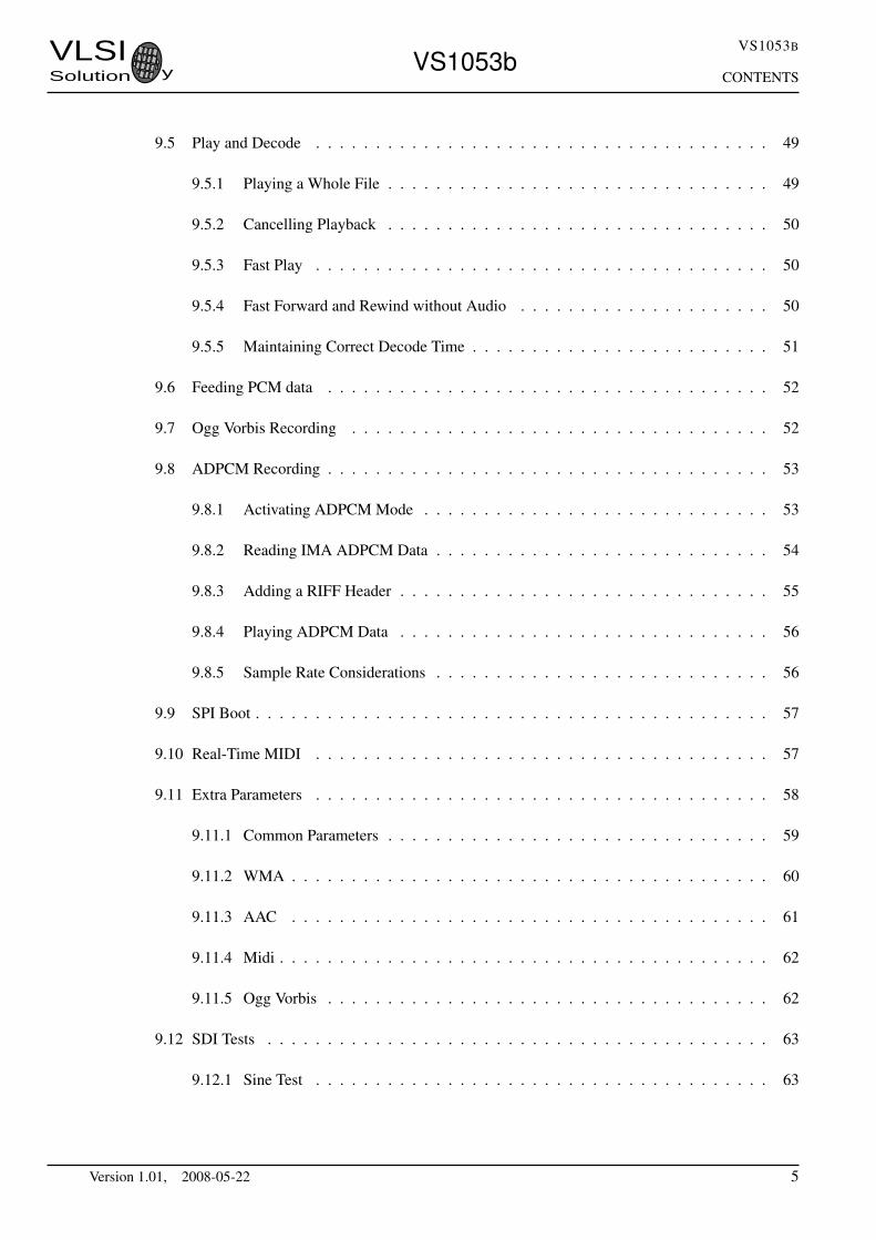
VLSISolution y VS1053b
VS1053B
CONTENTS
9.5 Play and Decode . . . . . . . . . . . . . . . . . . . . . . . . . . . . . . . . . . . . . . 49
9.5.1 Playing a Whole File . . . . . . . . . . . . . . . . . . . . . . . . . . . . . . . . 49
9.5.2 Cancelling Playback . . . . . . . . . . . . . . . . . . . . . . . . . . . . . . . . 50
9.5.3 Fast Play . . . . . . . . . . . . . . . . . . . . . . . . . . . . . . . . . . . . . . 50
9.5.4 Fast Forward and Rewind without Audio . . . . . . . . . . . . . . . . . . . . . 50
9.5.5 Maintaining Correct Decode Time . . . . . . . . . . . . . . . . . . . . . . . . . 51
9.6 Feeding PCM data . . . . . . . . . . . . . . . . . . . . . . . . . . . . . . . . . . . . . 52
9.7 Ogg Vorbis Recording . . . . . . . . . . . . . . . . . . . . . . . . . . . . . . . . . . . 52
9.8 ADPCM Recording . . . . . . . . . . . . . . . . . . . . . . . . . . . . . . . . . . . . . 53
9.8.1 Activating ADPCM Mode . . . . . . . . . . . . . . . . . . . . . . . . . . . . . 53
9.8.2 Reading IMA ADPCM Data . . . . . . . . . . . . . . . . . . . . . . . . . . . . 54
9.8.3 Adding a RIFF Header . . . . . . . . . . . . . . . . . . . . . . . . . . . . . . . 55
9.8.4 Playing ADPCM Data . . . . . . . . . . . . . . . . . . . . . . . . . . . . . . . 56
9.8.5 Sample Rate Considerations . . . . . . . . . . . . . . . . . . . . . . . . . . . . 56
9.9 SPI Boot . . . . . . . . . . . . . . . . . . . . . . . . . . . . . . . . . . . . . . . . . . . 57
9.10 Real-Time MIDI . . . . . . . . . . . . . . . . . . . . . . . . . . . . . . . . . . . . . . 57
9.11 Extra Parameters . . . . . . . . . . . . . . . . . . . . . . . . . . . . . . . . . . . . . . 58
9.11.1 Common Parameters . . . . . . . . . . . . . . . . . . . . . . . . . . . . . . . . 59
9.11.2 WMA . . . . . . . . . . . . . . . . . . . . . . . . . . . . . . . . . . . . . . . . 60
9.11.3 AAC . . . . . . . . . . . . . . . . . . . . . . . . . . . . . . . . . . . . . . . . 61
9.11.4 Midi . . . . . . . . . . . . . . . . . . . . . . . . . . . . . . . . . . . . . . . . . 62
9.11.5 Ogg Vorbis . . . . . . . . . . . . . . . . . . . . . . . . . . . . . . . . . . . . . 62
9.12 SDI Tests . . . . . . . . . . . . . . . . . . . . . . . . . . . . . . . . . . . . . . . . . . 63
9.12.1 Sine Test . . . . . . . . . . . . . . . . . . . . . . . . . . . . . . . . . . . . . . 63
Version 1.01, 2008-05-22 5

VLSISolution y VS1053b
VS1053B
CONTENTS
9.12.2 Pin Test . . . . . . . . . . . . . . . . . . . . . . . . . . . . . . . . . . . . . . . 63
9.12.3 SCI Test . . . . . . . . . . . . . . . . . . . . . . . . . . . . . . . . . . . . . . . 64
9.12.4 Memory Test . . . . . . . . . . . . . . . . . . . . . . . . . . . . . . . . . . . . 64
9.12.5 New Sine and Sweep Tests . . . . . . . . . . . . . . . . . . . . . . . . . . . . . 64
10 VS1053b Registers 66
10.1 Who Needs to Read This Chapter . . . . . . . . . . . . . . . . . . . . . . . . . . . . . 66
10.2 The Processor Core . . . . . . . . . . . . . . . . . . . . . . . . . . . . . . . . . . . . . 66
10.3 VS1053b Memory Map . . . . . . . . . . . . . . . . . . . . . . . . . . . . . . . . . . . 66
10.4 SCI Registers . . . . . . . . . . . . . . . . . . . . . . . . . . . . . . . . . . . . . . . . 66
10.5 Serial Data Registers . . . . . . . . . . . . . . . . . . . . . . . . . . . . . . . . . . . . 67
10.6 DAC Registers . . . . . . . . . . . . . . . . . . . . . . . . . . . . . . . . . . . . . . . 67
10.7 GPIO Registers . . . . . . . . . . . . . . . . . . . . . . . . . . . . . . . . . . . . . . . 67
10.8 Interrupt Registers . . . . . . . . . . . . . . . . . . . . . . . . . . . . . . . . . . . . . 68
10.9 Watchdog v1.0 2002-08-26 . . . . . . . . . . . . . . . . . . . . . . . . . . . . . . . . . . 69
10.9.1 Registers . . . . . . . . . . . . . . . . . . . . . . . . . . . . . . . . . . . . . . 69
10.10UART v1.1 2004-10-09 . . . . . . . . . . . . . . . . . . . . . . . . . . . . . . . . . . . 70
10.10.1 Registers . . . . . . . . . . . . . . . . . . . . . . . . . . . . . . . . . . . . . . 70
10.10.2 Status UARTx STATUS . . . . . . . . . . . . . . . . . . . . . . . . . . . . . . 70
10.10.3 Data UARTx DATA . . . . . . . . . . . . . . . . . . . . . . . . . . . . . . . . 71
10.10.4 Data High UARTx DATAH . . . . . . . . . . . . . . . . . . . . . . . . . . . . 71
10.10.5 Divider UARTx DIV . . . . . . . . . . . . . . . . . . . . . . . . . . . . . . . . 71
10.10.6 Interrupts and Operation . . . . . . . . . . . . . . . . . . . . . . . . . . . . . . 72
10.11Timers v1.0 2002-04-23 . . . . . . . . . . . . . . . . . . . . . . . . . . . . . . . . . . . 73
10.11.1 Registers . . . . . . . . . . . . . . . . . . . . . . . . . . . . . . . . . . . . . . 73
Version 1.01, 2008-05-22 6

VLSISolution y VS1053b
VS1053B
CONTENTS
10.11.2 Configuration TIMER CONFIG . . . . . . . . . . . . . . . . . . . . . . . . . . 73
10.11.3 Configuration TIMER ENABLE . . . . . . . . . . . . . . . . . . . . . . . . . . 74
10.11.4 Timer X Startvalue TIMER Tx[L/H] . . . . . . . . . . . . . . . . . . . . . . . 74
10.11.5 Timer X Counter TIMER TxCNT[L/H] . . . . . . . . . . . . . . . . . . . . . . 74
10.11.6 Interrupts . . . . . . . . . . . . . . . . . . . . . . . . . . . . . . . . . . . . . . 74
10.12VS1053b Audio Path . . . . . . . . . . . . . . . . . . . . . . . . . . . . . . . . . . . . 75
10.13I2S DAC Interface . . . . . . . . . . . . . . . . . . . . . . . . . . . . . . . . . . . . . 76
10.13.1 Registers . . . . . . . . . . . . . . . . . . . . . . . . . . . . . . . . . . . . . . 76
10.13.2 Configuration I2S CONFIG . . . . . . . . . . . . . . . . . . . . . . . . . . . . 76
11 VS1053 Version Changes 77
11.1 Changes Between VS1033c and VS1053a/b Firmware, 2007-03-08 . . . . . . . . . . . . 77
12 Document Version Changes 79
13 Contact Information 80
Version 1.01, 2008-05-22 7

VLSISolution y VS1053b
VS1053B
LIST OF FIGURES
List of Figures
1 Pin Configuration, LQFP-48. . . . . . . . . . . . . . . . . . . . . . . . . . . . . . . . . 13
2 VS1053b in LQFP-48 Packaging. . . . . . . . . . . . . . . . . . . . . . . . . . . . . . 13
3 Typical Connection Diagram Using LQFP-48. . . . . . . . . . . . . . . . . . . . . . . . 16
4 BSYNC Signal - one byte transfer. . . . . . . . . . . . . . . . . . . . . . . . . . . . . . 20
5 BSYNC Signal - two byte transfer. . . . . . . . . . . . . . . . . . . . . . . . . . . . . . 20
6 SCI Word Read . . . . . . . . . . . . . . . . . . . . . . . . . . . . . . . . . . . . . . . 21
7 SCI Word Write . . . . . . . . . . . . . . . . . . . . . . . . . . . . . . . . . . . . . . . 21
8 SCI Multiple Word Write . . . . . . . . . . . . . . . . . . . . . . . . . . . . . . . . . . 22
9 SPI Timing Diagram. . . . . . . . . . . . . . . . . . . . . . . . . . . . . . . . . . . . . 23
10 Two SCI Operations. . . . . . . . . . . . . . . . . . . . . . . . . . . . . . . . . . . . . 24
11 Two SDI Bytes. . . . . . . . . . . . . . . . . . . . . . . . . . . . . . . . . . . . . . . . 24
12 Two SDI Bytes Separated By an SCI Operation. . . . . . . . . . . . . . . . . . . . . . . 25
13 Data Flow of VS1053b. . . . . . . . . . . . . . . . . . . . . . . . . . . . . . . . . . . . 34
14 EarSpeaker externalized sound sources vs. normal inside-the-head sound . . . . . . . . . 35
15 RS232 Serial Interface Protocol . . . . . . . . . . . . . . . . . . . . . . . . . . . . . . 70
16 VS1053b ADC and DAC data paths . . . . . . . . . . . . . . . . . . . . . . . . . . . . 75
17 I2S Interface, 192 kHz. . . . . . . . . . . . . . . . . . . . . . . . . . . . . . . . . . . . 76
Version 1.01, 2008-05-22 8
VLSISolution y VS1053b
VS1053B
1. LICENSES
1 Licenses
MPEG Layer-3 audio decoding technology licensed from Fraunhofer IIS and Thomson.
Note: If you enable Layer I and Layer II decoding, you are liable for any patent issues that mayarise from using these formats. Joint licensing of MPEG 1.0 / 2.0 Layer III does not cover all patentspertaining to layers I and II.
VS1053b contains WMA decoding technology from Microsoft.This product is protected by certain intellectual property rights of Microsoft and cannot be usedor further distributed without a license from Microsoft.
VS1053b contains AAC technology (ISO/IEC 13818-7 and ISO/IEC 14496-3) which cannot be usedwithout a proper license from Via Licensing Corporation or individual patent holders.
VS1053b contains spectral band replication (SBR) and parametric stereo (PS) technologies developed byCoding Technologies. Licensing of SBR is handled within MPEG4 through Via Licensing Corporation.Licensing of PS is handled with Coding Technologies.See http://www.codingtechnologies.com/licensing/aacplus.htm for more information.
To the best of our knowledge, if the end product does not play a specific format that otherwise wouldrequire a customer license: MPEG 1.0/2.0 layers I and II, WMA, or AAC, the respective license shouldnot be required. Decoding of MPEG layers I and II are disabled by default, and WMA and AAC formatexclusion can be easily performed based on the contents of the SCI HDAT1 register. Also PS and SBRdecoding can be separately disabled.
2 Disclaimer
This is a preliminary datasheet. All properties and figures are subject to change.
3 Definitions
B Byte, 8 bits.
b Bit.
Ki “Kibi” = 210 = 1024 (IEC 60027-2).
Mi “Mebi” = 220 = 1048576 (IEC 60027-2).
VS DSP VLSI Solution’s DSP core.
W Word. In VS DSP, instruction words are 32-bit and data words are 16-bit wide.
Version 1.01, 2008-05-22 9

VLSISolution y VS1053b
VS1053B
4. CHARACTERISTICS & SPECIFICATIONS
4 Characteristics & Specifications
4.1 Absolute Maximum Ratings
Parameter Symbol Min Max UnitAnalog Positive Supply AVDD -0.3 3.6 VDigital Positive Supply CVDD -0.3 1.85 VI/O Positive Supply IOVDD -0.3 3.6 VCurrent at Any Non-Power Pin1 ±50 mAVoltage at Any Digital Input -0.3 IOVDD+0.32 VOperating Temperature -30 +85 CStorage Temperature -65 +150 C
1 Higher current can cause latch-up.2 Must not exceed 3.6 V
4.2 Recommended Operating Conditions
Parameter Symbol Min Typ Max UnitAmbient Operating Temperature -30 +85 CAnalog and Digital Ground 1 AGND DGND 0.0 VPositive Analog, REF=1.23V AVDD 2.5 2.8 3.6 VPositive Analog, REF=1.65V 2 AVDD 3.3 3.3 3.6 VPositive Digital CVDD 1.7 1.8 1.85 VI/O Voltage IOVDD 1.8 2.8 3.6 VInput Clock Frequency 3 XTALI 12 12.288 13 MHzInternal Clock Frequency CLKI 12 36.864 55.3 MHzInternal Clock Multiplier 4 1.0× 3.0× 4.5×Master Clock Duty Cycle 40 50 60 %
1 Must be connected together as close the device as possible for latch-up immunity.2 Reference voltage can be internally selected between 1.23V and 1.65V, see section 8.7.2.3 The maximum sample rate that can be played with correct speed is XTALI/256 (or XTALI/512 ifSM CLK RANGE is set). Thus, XTALI must be at least 12.288 MHz (24.576 MHz) to be able to play48 kHz at correct speed.4 Reset value is 1.0×. Recommended SC MULT=3.5×, SC ADD=1.0× (SCI CLOCKF=0x8800).Do not exceed maximum specification for CLKI.
Version 1.01, 2008-05-22 10

VLSISolution y VS1053b
VS1053B
4. CHARACTERISTICS & SPECIFICATIONS
4.3 Analog Characteristics
Unless otherwise noted: AVDD=3.3V, CVDD=1.8V, IOVDD=2.8V, REF=1.65V, TA=-30..+85C,XTALI=12..13MHz, Internal Clock Multiplier 3.5×. DAC tested with 1307.894 Hz full-scale outputsinewave, measurement bandwidth 20..20000 Hz, analog output load: LEFT to GBUF 30 Ω, RIGHT toGBUF 30 Ω. Microphone test amplitude 48 mVpp, fs=1 kHz, Line input test amplitude 1.26 V, fs=1 kHz.
Parameter Symbol Min Typ Max UnitDAC Resolution 18 bitsTotal Harmonic Distortion THD 0.07 %Third Harmonic Distortion 0.02 %Dynamic Range (DAC unmuted, A-weighted) IDR 100 dBS/N Ratio (full scale signal) SNR 94 dBInterchannel Isolation (Cross Talk), 600Ω + GBUF 80 dBInterchannel Isolation (Cross Talk), 30Ω + GBUF 53 dBInterchannel Gain Mismatch -0.5 0.5 dBFrequency Response -0.1 0.1 dBFull Scale Output Voltage (Peak-to-peak) 1.64 1.851 2.06 VppDeviation from Linear Phase 5
Analog Output Load Resistance AOLR 16 302 ΩAnalog Output Load Capacitance 100 pFMicrophone input amplifier gain MICG 26 dBMicrophone input amplitude 48 1403 mVpp ACMicrophone Total Harmonic Distortion MTHD 0.03 0.07 %Microphone S/N Ratio MSNR 60 70 dBMicrophone input impedances, per pin 45 kΩLine input amplitude 2500 28003 mVpp ACLine input Total Harmonic Distortion LTHD 0.005 0.014 %Line input S/N Ratio LSNR 85 90 dBLine input impedance 80 kΩ
1 3.0 volts can be achieved with +-to-+ wiring for mono difference sound.2 AOLR may be much lower, but below Typical distortion performance may be compromised.3 Above typical amplitude the Harmonic Distortion increases.
Version 1.01, 2008-05-22 11
VLSISolution y VS1053b
VS1053B
4. CHARACTERISTICS & SPECIFICATIONS
4.4 Power Consumption
Tested with an MPEG 1.0 Layer-3 128 kbps sample and generated sine. Output at full volume. Internalclock multiplier 3.0×. TA=+25C.
Parameter Min Typ Max UnitPower Supply Consumption AVDD, Reset 0.6 5.0 µAPower Supply Consumption CVDD = 1.8V, Reset 12 20.0 µAPower Supply Consumption AVDD, sine test, 30 Ω + GBUF 30 36.9 60 mAPower Supply Consumption CVDD = 1.8V, sine test 8 10 15 mAPower Supply Consumption AVDD, no load 5 mAPower Supply Consumption AVDD, output load 30 Ω 11 mAPower Supply Consumption AVDD, 30 Ω + GBUF 11 mAPower Supply Consumption CVDD = 1.8V 11 mA
4.5 Digital Characteristics
Parameter Min Max UnitHigh-Level Input Voltage 0.7×CVDD IOVDD+0.31 VLow-Level Input Voltage -0.2 0.3×CVDD VHigh-Level Output Voltage at XTALO = -0.1 mA 0.7×IOVDD VLow-Level Output Voltage at XTALO = 0.1 mA 0.3×IOVDD VHigh-Level Output Voltage at IO = -1.0 mA 0.7×IOVDD VLow-Level Output Voltage at IO = 1.0 mA 0.3×IOVDD VInput Leakage Current -1.0 1.0 µASPI Input Clock Frequency 2 CLKI
7 MHzRise time of all output pins, load = 50 pF 50 ns
1 Must not exceed 3.6V2 Value for SCI reads. SCI and SDI writes allow CLKI
4 .
4.6 Switching Characteristics - Boot Initialization
Parameter Symbol Min Max UnitXRESET active time 2 XTALIXRESET inactive to software ready 22000 500001 XTALIPower on reset, rise time to CVDD 10 V/s
1 DREQ rises when initialization is complete. You should not send any data or commands before that.
Version 1.01, 2008-05-22 12

VLSISolution y VS1053b
VS1053B
5. PACKAGES AND PIN DESCRIPTIONS
5 Packages and Pin Descriptions
5.1 Packages
LPQFP-48 is a lead (Pb) free and also RoHS compliant package. RoHS is a short name of Directive2002/95/EC on the restriction of the use of certain hazardous substances in electrical and electronicequipment.
5.1.1 LQFP-48
148
Figure 1: Pin Configuration, LQFP-48.
LQFP-48 package dimensions are at http://www.vlsi.fi/ .
Figure 2: VS1053b in LQFP-48 Packaging.
Version 1.01, 2008-05-22 13

VLSISolution y VS1053b
VS1053B
5. PACKAGES AND PIN DESCRIPTIONS
Pad Name LQFPPin
PinType
Function
MICP / LINE1 1 AI Positive differential mic input, self-biasing / Line-in 1MICN 2 AI Negative differential mic input, self-biasingXRESET 3 DI Active low asynchronous reset, schmitt-trigger inputDGND0 4 DGND Core & I/O groundCVDD0 5 CPWR Core power supplyIOVDD0 6 IOPWR I/O power supplyCVDD1 7 CPWR Core power supplyDREQ 8 DO Data request, input busGPIO2 / DCLK1 9 DIO General purpose IO 2 / serial input data bus clockGPIO3 / SDATA1 10 DIO General purpose IO 3 / serial data inputGPIO6 / I2S SCLK3 11 DIO General purpose IO 6 / I2S SCLKGPIO7 / I2S SDATA3 12 DIO General purpose IO 7 / I2S SDATAXDCS / BSYNC1 13 DI Data chip select / byte syncIOVDD1 14 IOPWR I/O power supplyVCO 15 DO For testing only (Clock VCO output)DGND1 16 DGND Core & I/O groundXTALO 17 AO Crystal outputXTALI 18 AI Crystal inputIOVDD2 19 IOPWR I/O power supplyDGND2 20 DGND Core & I/O groundDGND3 21 DGND Core & I/O groundDGND4 22 DGND Core & I/O groundXCS 23 DI Chip select input (active low)CVDD2 24 CPWR Core power supplyGPIO5 / I2S MCLK3 25 DIO General purpose IO 5 / I2S MCLKRX 26 DI UART receive, connect to IOVDD if not usedTX 27 DO UART transmitSCLK 28 DI Clock for serial busSI 29 DI Serial inputSO 30 DO3 Serial outputCVDD3 31 CPWR Core power supplyXTEST 32 DI Reserved for test, connect to IOVDDGPIO0 33 DIO Gen. purp. IO 0 (SPIBOOT), use 100 kΩ pull-down resistor2
GPIO1 34 DIO General purpose IO 1GND 35 DGND I/O GroundGPIO4 / I2S LROUT3 36 DIO General purpose IO 4 / I2S LROUTAGND0 37 APWR Analog ground, low-noise referenceAVDD0 38 APWR Analog power supplyRIGHT 39 AO Right channel outputAGND1 40 APWR Analog groundAGND2 41 APWR Analog groundGBUF 42 AO Common buffer for headphones, do NOT connect to ground!AVDD1 43 APWR Analog power supplyRCAP 44 AIO Filtering capacitance for referenceAVDD2 45 APWR Analog power supplyLEFT 46 AO Left channel outputAGND3 47 APWR Analog groundLINE2 48 AI Line-in 2 (right channel)
1 First pin function is active in New Mode, latter in Compatibility Mode.2 Unless pull-down resistor is used, SPI Boot is tried. See Chapter 9.9 for details.3 If I2S CF ENA is ’0’ the pins are used for GPIO. See Chapter 10.13 for details.
Version 1.01, 2008-05-22 14

VLSISolution y VS1053b
VS1053B
5. PACKAGES AND PIN DESCRIPTIONS
Pin types:
Type DescriptionDI Digital input, CMOS Input PadDO Digital output, CMOS Input PadDIO Digital input/outputDO3 Digital output, CMOS Tri-stated Output PadAI Analog input
Type DescriptionAO Analog outputAIO Analog input/outputAPWR Analog power supply pinDGND Core or I/O ground pinCPWR Core power supply pinIOPWR I/O power supply pin
Version 1.01, 2008-05-22 15

VLSISolution y VS1053b
VS1053B
6. CONNECTION DIAGRAM, LQFP-48
6 Connection Diagram, LQFP-48
Figure 3: Typical Connection Diagram Using LQFP-48.
Figure 3 shows a typical connection diagram for VS1053.
Figure Note 1: Connect either Microphone In or Line In, but not both at the same time.
Note: This connection assumes SM SDINEW is active (see Chapter 8.7.1). If also SM SDISHARE isused, xDCS should be tied low or high (see Chapter 7.2.1).
Version 1.01, 2008-05-22 16

VLSISolution y VS1053b
VS1053B
6. CONNECTION DIAGRAM, LQFP-48
The common buffer GBUF can be used for common voltage (1.23 V) for earphones. This will eliminatethe need for large isolation capacitors on line outputs, and thus the audio output pins from VS1053b maybe connected directly to the earphone connector.
GBUF must NOT be connected to ground under any circumstances. If GBUF is not used, LEFT andRIGHT must be provided with coupling capacitors. To keep GBUF stable, you should always have theresistor and capacitor even when GBUF is not used. See application notes for details.
Unused GPIO pins should have a pull-down resistor. Unused line and microphone inputs should not beconnected.
If UART is not used, RX should be connected to IOVDD and TX be unconnected.
Do not connect any external load to XTALO.
Version 1.01, 2008-05-22 17

VLSISolution y VS1053b
VS1053B
7. SPI BUSES
7 SPI Buses
7.1 General
The SPI Bus - that was originally used in some Motorola devices - has been used for both VS1053b’sSerial Data Interface SDI (Chapters 7.4 and 8.5) and Serial Control Interface SCI (Chapters 7.5 and 8.6).
7.2 SPI Bus Pin Descriptions
7.2.1 VS1002 Native Modes (New Mode)
These modes are active on VS1053b when SM SDINEW is set to 1 (default at startup). DCLK andSDATA are not used for data transfer and they can be used as general-purpose I/O pins (GPIO2 andGPIO3). BSYNC function changes to data interface chip select (XDCS).
SDI Pin SCI Pin DescriptionXDCS XCS Active low chip select input. A high level forces the serial interface into
standby mode, ending the current operation. A high level also forces serialoutput (SO) to high impedance state. If SM SDISHARE is 1, pinXDCS is not used, but the signal is generated internally by invertingXCS.
SCK Serial clock input. The serial clock is also used internally as the masterclock for the register interface.SCK can be gated or continuous. In either case, the first rising clock edgeafter XCS has gone low marks the first bit to be written.
SI Serial input. If a chip select is active, SI is sampled on the rising CLK edge.- SO Serial output. In reads, data is shifted out on the falling SCK edge.
In writes SO is at a high impedance state.
7.2.2 VS1001 Compatibility Mode (deprecated)
This mode is active when SM SDINEW is set to 0. In this mode, DCLK, SDATA and BSYNC are active.
SDI Pin SCI Pin Description- XCS Active low chip select input. A high level forces the serial interface into
standby mode, ending the current operation. A high level also forces serialoutput (SO) to high impedance state.
BSYNC - SDI data is synchronized with a rising edge of BSYNC.DCLK SCK Serial clock input. The serial clock is also used internally as the master
clock for the register interface.SCK can be gated or continuous. In either case, the first rising clock edgeafter XCS has gone low marks the first bit to be written.
SDATA SI Serial input. SI is sampled on the rising SCK edge, if XCS is low.- SO Serial output. In reads, data is shifted out on the falling SCK edge.
In writes SO is at a high impedance state.
Version 1.01, 2008-05-22 18

VLSISolution y VS1053b
VS1053B
7. SPI BUSES
7.3 Data Request Pin DREQ
The DREQ pin/signal is used to signal if VS1053b’s 2048-byte FIFO is capable of receiving data. IfDREQ is high, VS1053b can take at least 32 bytes of SDI data or one SCI command. DREQ is turnedlow when the stream buffer is too full and for the duration of a SCI command.
Because of the 32-byte safety area, the sender may send upto 32 bytes of SDI data at a time withoutchecking the status of DREQ, making controlling VS1053b easier for low-speed microcontrollers.
Note: DREQ may turn low or high at any time, even during a byte transmission. Thus, DREQ shouldonly be used to decide whether to send more bytes. It does not need to abort a transmission that hasalready started.
Note: In VS10XX products upto VS1002, DREQ was only used for SDI. In VS1053b DREQ is alsoused to tell the status of SCI.
There are cases when you still want to send SCI commands when DREQ is low. Because DREQ isshared between SDI and SCI, you can not determine if a SCI command has been executed if SDI is notready to receive. In this case you need a long enough delay after every SCI command to make certainnone of them is missed. The SCI Registers table in section 8.7 gives the worst-case handling time foreach SCI register write.
7.4 Serial Protocol for Serial Data Interface (SDI)
7.4.1 General
The serial data interface operates in slave mode so DCLK signal must be generated by an external circuit.
Data (SDATA signal) can be clocked in at either the rising or falling edge of DCLK (Chapter 8.7).
VS1053b assumes its data input to be byte-sychronized. SDI bytes may be transmitted either MSb orLSb first, depending of contents of SCI MODE (Chapter 8.7.1).
The firmware is able to accept the maximum bitrate the SDI supports.
7.4.2 SDI in VS1002 Native Modes (New Mode)
In VS1002 native modes (SM NEWMODE is 1), byte synchronization is achieved by XDCS. The state ofXDCS may not change while a data byte transfer is in progress. To always maintain data synchronizationeven if there may be glitches in the boards using VS1053b, it is recommended to turn XDCS every nowand then, for instance once after every disk data block, just to make sure the host and VS1053b are insync.
If SM SDISHARE is 1, the XDCS signal is internally generated by inverting the XCS input.
For new designs, using VS1002 native modes are recommended.
Version 1.01, 2008-05-22 19
VLSISolution y VS1053b
VS1053B
7. SPI BUSES
7.4.3 SDI in VS1001 Compatibility Mode (deprecated)
BSYNC
SDATA
DCLK
D7 D6 D5 D4 D3 D2 D1 D0
Figure 4: BSYNC Signal - one byte transfer.
When VS1053b is running in VS1001 compatibility mode, a BSYNC signal must be generated to ensurecorrect bit-alignment of the input bitstream. The first DCLK sampling edge (rising or falling, dependingon selected polarity), during which the BSYNC is high, marks the first bit of a byte (LSB, if LSB-firstorder is used, MSB, if MSB-first order is used). If BSYNC is ’1’ when the last bit is received, the receiverstays active and next 8 bits are also received.
BSYNC
SDATA
DCLK
D7 D6 D5 D4 D3 D2 D1 D0 D7 D6 D5 D4 D3 D2 D1 D0
Figure 5: BSYNC Signal - two byte transfer.
7.4.4 Passive SDI Mode
If SM NEWMODE is 0 and SM SDISHARE is 1, the operation is otherwise like the VS1001 compat-ibility mode, but bits are only received while the BSYNC signal is ’1’. Rising edge of BSYNC is stillused for synchronization.
7.5 Serial Protocol for Serial Command Interface (SCI)
7.5.1 General
The serial bus protocol for the Serial Command Interface SCI (Chapter 8.6) consists of an instructionbyte, address byte and one 16-bit data word. Each read or write operation can read or write a singleregister. Data bits are read at the rising edge, so the user should update data at the falling edge. Bytesare always send MSb first. XCS should be low for the full duration of the operation, but you can havepauses between bits if needed.
The operation is specified by an 8-bit instruction opcode. The supported instructions are read and write.See table below.
InstructionName Opcode OperationREAD 0b0000 0011 Read dataWRITE 0b0000 0010 Write data
Note: VS1053b sets DREQ low after each SCI operation. The duration depends on the operation. It isnot allowed to finish a new SCI/SDI operation before DREQ is high again.
Version 1.01, 2008-05-22 20

VLSISolution y VS1053b
VS1053B
7. SPI BUSES
7.5.2 SCI Read
0 1 2 3 4 5 6 7 8 9 10 11 12 13 30 3114 15 16 17
0 0 0 0 0 0 1 1 0 0 0 03 2 1 0
0 0 0 0 0 0 0 0 0 0 0 0 0 0 0 015 14 1 0
X
instruction (read) address data out
XCS
SCK
SI
SO
don’t care don’t care
DREQ
execution
Figure 6: SCI Word Read
VS1053b registers are read from using the following sequence, as shown in Figure 6. First, XCS line ispulled low to select the device. Then the READ opcode (0x3) is transmitted via the SI line followed byan 8-bit word address. After the address has been read in, any further data on SI is ignored by the chip.The 16-bit data corresponding to the received address will be shifted out onto the SO line.
XCS should be driven high after data has been shifted out.
DREQ is driven low for a short while when in a read operation by the chip. This is a very short time anddoesn’t require special user attention.
7.5.3 SCI Write
0 1 2 3 4 5 6 7 8 9 10 11 12 13 30 3114 15 16 17
0 0 0 0 0 0 1 0 0 0 03 2 1 0 1 0
X
address
XCS
SCK
SI
15 14
data out
0 0 0 0 0 0 0 0 0 0 0 0 0 0 0 0SO 0 0 0 0 X
0
instruction (write)
DREQ
execution
Figure 7: SCI Word Write
VS1053b registers are written from using the following sequence, as shown in Figure 7. First, XCS lineis pulled low to select the device. Then the WRITE opcode (0x2) is transmitted via the SI line followedby an 8-bit word address.
Version 1.01, 2008-05-22 21

VLSISolution y VS1053b
VS1053B
7. SPI BUSES
After the word has been shifted in and the last clock has been sent, XCS should be pulled high to end theWRITE sequence.
After the last bit has been sent, DREQ is driven low for the duration of the register update, marked“execution” in the figure. The time varies depending on the register and its contents (see table in Chap-ter 8.7 for details). If the maximum time is longer than what it takes from the microcontroller to feedthe next SCI command or SDI byte, status of DREQ must be checked before finishing the next SCI/SDIoperation.
7.5.4 SCI Multiple Write
0 1 2 3 4 5 6 7 8 9 10 11 12 13 14 15 16 17
0 0 0 0 0 0 1 0 0 0 03 2 1 0
address
XCS
SCK
SI
15 14
0 0 0 0 0 0 0 0 0 0 0 0 0 0 0 0SO 0 0
0
instruction (write)
DREQ
1 0X
0 0 X
execution
1 0 15 14
data out 1 data out 2
0 0 0 0
execution
X
3130 32 3329
d.out n
m−2m−1
Figure 8: SCI Multiple Word Write
VS1053b allows for the user to send multiple words to the same SCI register, which allows fast SCIuploads, shown in Figure 8. The main difference to a single write is that instead of bringing XCS upafter sending the last bit of a data word, the next data word is sent immediately. After the last data word,XCS is driven high as with a single word write.
After the last bit of a word has been sent, DREQ is driven low for the duration of the register update,marked “execution” in the figure. The time varies depending on the register and its contents (see tablein Chapter 8.7 for details). If the maximum time is longer than what it takes from the microcontrollerto feed the next SCI command or SDI byte, status of DREQ must be checked before finishing the nextSCI/SDI operation.
Version 1.01, 2008-05-22 22

VLSISolution y VS1053b
VS1053B
7. SPI BUSES
7.6 SPI Timing Diagram
XCS
SCK
SI
SO
0 1 1514 16
tXCSS tXCSHtWL tWH
tHtSU
tV
tZ
tDIS
tXCS30 31
Figure 9: SPI Timing Diagram.
Symbol Min Max UnittXCSS 5 nstSU 0 nstH 2 CLKI cyclestZ 0 nstWL 2 CLKI cyclestWH 2 CLKI cyclestV 2 (+ 25 ns1) CLKI cyclestXCSH 1 CLKI cyclestXCS 2 CLKI cyclestDIS 10 ns
1 25 ns is when pin loaded with 100 pF capacitance. The time is shorter with lower capacitance.
Note: Although the timing is derived from the internal clock CLKI, the system always starts up in 1.0×mode, thus CLKI=XTALI. After you have configured a higher clock through SCI CLOCKF and waitedfor DREQ to rise, you can use a higher SPI speed as well.
Note: Because tWL + tWH + tH is 6×CLKI + 25 ns, the maximum speed for SCI reads is CLKI/7.
Version 1.01, 2008-05-22 23

VLSISolution y VS1053b
VS1053B
7. SPI BUSES
7.7 SPI Examples with SM SDINEW and SM SDISHARED set
7.7.1 Two SCI Writes
0 1 2 3 30 31
1 0 1 0
0 0 0 0 0 0X X
XCS
SCK
SI
2
32 33 61 62 63
SCI Write 1 SCI Write 2
DREQ
DREQ up before finishing next SCI write
Figure 10: Two SCI Operations.
Figure 10 shows two consecutive SCI operations. Note that xCS must be raised to inactive state betweenthe writes. Also DREQ must be respected as shown in the figure.
7.7.2 Two SDI Bytes
1 2 3
XCS
SCK
SI
7 6 5 4 3 1 0 7 6 5 2 1 0
X
SDI Byte 1SDI Byte 2
0 6 7 8 9 13 14 15
DREQ
Figure 11: Two SDI Bytes.
SDI data is synchronized with a raising edge of xCS as shown in Figure 11. However, every byte doesn’tneed separate synchronization.
Version 1.01, 2008-05-22 24

VLSISolution y VS1053b
VS1053B
7. SPI BUSES
7.7.3 SCI Operation in Middle of Two SDI Bytes
0 1
XCS
SCK
SI
7
7 6 5 1
0 0
0 7 6 5 1 0
SDI ByteSCI Operation
SDI Byte
8 9 39 40 41 46 47
X
DREQ high before end of next transfer
DREQ
Figure 12: Two SDI Bytes Separated By an SCI Operation.
Figure 12 shows how an SCI operation is embedded in between SDI operations. xCS edges are used tosynchronize both SDI and SCI. Remember to respect DREQ as shown in the figure.
Version 1.01, 2008-05-22 25
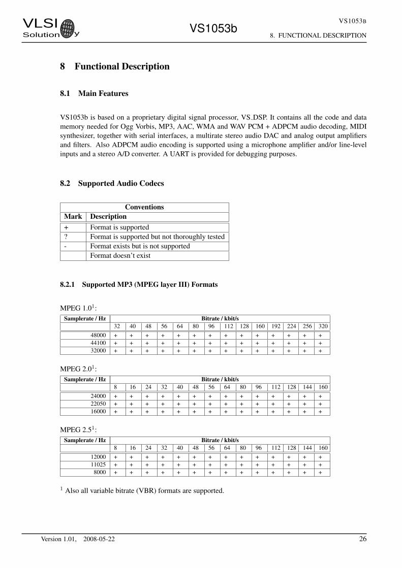
VLSISolution y VS1053b
VS1053B
8. FUNCTIONAL DESCRIPTION
8 Functional Description
8.1 Main Features
VS1053b is based on a proprietary digital signal processor, VS DSP. It contains all the code and datamemory needed for Ogg Vorbis, MP3, AAC, WMA and WAV PCM + ADPCM audio decoding, MIDIsynthesizer, together with serial interfaces, a multirate stereo audio DAC and analog output amplifiersand filters. Also ADPCM audio encoding is supported using a microphone amplifier and/or line-levelinputs and a stereo A/D converter. A UART is provided for debugging purposes.
8.2 Supported Audio Codecs
ConventionsMark Description+ Format is supported? Format is supported but not thoroughly tested- Format exists but is not supported
Format doesn’t exist
8.2.1 Supported MP3 (MPEG layer III) Formats
MPEG 1.01:Samplerate / Hz Bitrate / kbit/s
32 40 48 56 64 80 96 112 128 160 192 224 256 32048000 + + + + + + + + + + + + + +44100 + + + + + + + + + + + + + +32000 + + + + + + + + + + + + + +
MPEG 2.01:Samplerate / Hz Bitrate / kbit/s
8 16 24 32 40 48 56 64 80 96 112 128 144 16024000 + + + + + + + + + + + + + +22050 + + + + + + + + + + + + + +16000 + + + + + + + + + + + + + +
MPEG 2.51:Samplerate / Hz Bitrate / kbit/s
8 16 24 32 40 48 56 64 80 96 112 128 144 16012000 + + + + + + + + + + + + + +11025 + + + + + + + + + + + + + +
8000 + + + + + + + + + + + + + +
1 Also all variable bitrate (VBR) formats are supported.
Version 1.01, 2008-05-22 26

VLSISolution y VS1053b
VS1053B
8. FUNCTIONAL DESCRIPTION
8.2.2 Supported MP1 (MPEG layer I) Formats
Note: Layer I / II decoding must be specifically enabled from register SCI MODE.
MPEG 1.0:Samplerate / Hz Bitrate / kbit/s
32 64 96 128 160 192 224 256 288 320 352 384 416 44848000 + + + + + + + + + + + + + +44100 + + + + + + + + + + + + + +32000 + + + + + + + + + + + + + +
MPEG 2.0:Samplerate / Hz Bitrate / kbit/s
32 48 56 64 80 96 112 128 144 160 176 192 224 25624000 ? ? ? ? ? ? ? ? ? ? ? ? ? ?22050 ? ? ? ? ? ? ? ? ? ? ? ? ? ?16000 ? ? ? ? ? ? ? ? ? ? ? ? ? ?
8.2.3 Supported MP2 (MPEG layer II) Formats
Note: Layer I / II decoding must be specifically enabled from register SCI MODE.
MPEG 1.0:Samplerate / Hz Bitrate / kbit/s
32 48 56 64 80 96 112 128 160 192 224 256 320 38448000 + + + + + + + + + + + + + +44100 + + + + + + + + + + + + + +32000 + + + + + + + + + + + + + +
MPEG 2.0:Samplerate / Hz Bitrate / kbit/s
8 16 24 32 40 48 56 64 80 96 112 128 144 16024000 + + + + + + + + + + + + + +22050 + + + + + + + + + + + + + +16000 + + + + + + + + + + + + + +
8.2.4 Supported Ogg Vorbis Formats
Parameter Min Max UnitChannels 2Window size 64 4096 samplesSamplerate 48000 HzBitrate 500 kbit/sec
Only floor 1 is supported. No known current encoder uses floor 0. All one- and two-channel Ogg Vorbisfiles should be playable with this decoder.
Version 1.01, 2008-05-22 27

VLSISolution y VS1053b
VS1053B
8. FUNCTIONAL DESCRIPTION
8.2.5 Supported AAC (ISO/IEC 13818-7 and ISO/IEC 14496-3) Formats
VS1053b decodes MPEG2-AAC-LC-2.0.0.0 and MPEG4-AAC-LC-2.0.0.0 streams, i.e. the low com-plexity profile with maximum of two channels can be decoded. If a stream contains more than oneelement and/or element type, you can select which one to decode from the 16 single-channel, 16 channel-pair, and 16 low-frequency elements. The default is to select the first one that appears in the stream.
Dynamic range control (DRC) is supported and can be controlled by the user to limit or enhance thedynamic range of the material that contains DRC information.
Both Sine window and Kaiser-Bessel-derived window are supported.
For MPEG4 pseudo-random noise substitution (PNS) is supported. Short frames (120 and 960 samples)are not supported.
Spectral Band Replication (SBR) level 3, and Parametric Stereo (PS) level 3 are supported (HE-AAC v2).Level 3 means that maximum of 2 channels, samplerates upto and including 48 kHz without and withSBR (with or without PS) are supported. Also, both mixing modes (Ra and Rb), IPD/OPD synthesisand 34 frequency bands resolution are implemented. The downsampled synthesis mode (core codersamplerates > 24 kHz and <= 48 kHz with SBR) is implemented.
SBR and PS decoding can also be disabled. Also different operating modes can be selected. Seeconfig1 and sbrAndPsStatus in section 9.11 : ”Extra parameters”.
If enabled, the internal clock (CLKI) is automatically increased if AAC decoding needs a higher clock.PS and SBR operation is automatically switched off if the internal clock is too slow for correct decoding.Generally HE-AAC v2 files need 4.5× clock to decode both SBR and PS content. This is why 3.5× +1.0× clock is the recommended default.
For AAC the streaming ADTS format is recommended. This format allows easy rewind and fast forwardbecause resynchronization is easily possible.
In addition to ADTS (.aac), MPEG2 ADIF (.aac) and MPEG4 AUDIO (.mp4 / .m4a) files are played,but these formats are less suitable for rewind and fast forward operations. You can still implement thesefeatures by using the safe jump points table, or using slightly less robust but much easier automaticresync mechanism (see Section 9.5.4).
Because 3GPP (.3gp) and 3GPPv2 (.3g2) files are just MPEG4 files, those that contain only HE-AAC orHE-AACv2 content are played.
Note: To be able to play the .3gp, .3g2, .mp4 and .m4a files, the mdat atom must be the last atom inthe MP4 file. Because VS1053b receives all data as a stream, all metadata must be available before themusic data is received. Several MP4 file formatters do not satisfy this requirement and some kind ofconversion is required. This is also why the streamable ADTS format is recommended.
Programs exist that optimize the .mp4 and .m4a into so-called streamable format that has the mdat atomlast in the file, and thus suitable for web servers’ audio streaming. You can use this kind of tool to processfiles for VS1053b too. For example mp4creator -optimize file.mp4.
Version 1.01, 2008-05-22 28

VLSISolution y VS1053b
VS1053B
8. FUNCTIONAL DESCRIPTION
AAC12:
Samplerate / Hz Maximum Bitrate kbit/s - for 2 channels≤96 132 144 192 264 288 384 529 576
48000 + + + + + + + + +44100 + + + + + + + +32000 + + + + + + +24000 + + + + + +22050 + + + + +16000 + + + +12000 + + +11025 + +
8000 +
1 64000 Hz, 88200 Hz, and 96000 Hz AAC files are played at the highest possible samplerate (48000 Hzwith 12.288 MHz XTALI).
2 Also all variable bitrate (VBR) formats are supported. Note that the table gives the maximum bitrateallowed for two channels for a specific samplerate as defined by the AAC specification. The decoderdoes not actually have a fixed lower or upper limit.
Version 1.01, 2008-05-22 29

VLSISolution y VS1053b
VS1053B
8. FUNCTIONAL DESCRIPTION
8.2.6 Supported WMA Formats
Windows Media Audio codec versions 2, 7, 8, and 9 are supported. All WMA profiles (L1, L2, and L3)are supported. Previously streams were separated into Classes 1, 2a, 2b, and 3. The decoder has passedMicrosoft’s conformance testing program. Windows Media Audio Professional is a different codec andis not supported.
WMA 4.0 / 4.1:Samplerate Bitrate / kbit/s
/ Hz 5 6 8 10 12 16 20 22 32 40 48 64 80 96 128 160 1928000 + + + +
11025 + +16000 + + + +22050 + + + +32000 + + + + + +44100 + + + + + + +48000 + +
WMA 7:Samplerate Bitrate / kbit/s
/ Hz 5 6 8 10 12 16 20 22 32 40 48 64 80 96 128 160 1928000 + + + +
11025 + +16000 + + + +22050 + + + +32000 + + + +44100 + + + + + + + +48000 + +
WMA 8:Samplerate Bitrate / kbit/s
/ Hz 5 6 8 10 12 16 20 22 32 40 48 64 80 96 128 160 1928000 + + + +
11025 + +16000 + + + +22050 + + + +32000 + + + +44100 + + + + + + + +48000 + + +
WMA 9:Samplerate Bitrate / kbit/s
/ Hz 5 6 8 10 12 16 20 22 32 40 48 64 80 96 128 160 192 256 3208000 + + + +
11025 + +16000 + + + +22050 + + + +32000 + + + +44100 + + + + + + + + + + +48000 + + + + +
In addition to these expected WMA decoding profiles, all other bitrate and samplerate combinations aresupported, including variable bitrate WMA streams. Note that WMA does not consume the bitstream asevenly as MP3, so you need a higher peak transfer capability for clean playback at the same bitrate.
Version 1.01, 2008-05-22 30
VLSISolution y VS1053b
VS1053B
8. FUNCTIONAL DESCRIPTION
8.2.7 Supported RIFF WAV Formats
The most common RIFF WAV subformats are supported, with 1 or 2 audio channels.
Format Name Supported Comments0x01 PCM + 16 and 8 bits, any samplerate ≤ 48kHz0x02 ADPCM -0x03 IEEE FLOAT -0x06 ALAW -0x07 MULAW -0x10 OKI ADPCM -0x11 IMA ADPCM + Any samplerate ≤ 48kHz0x15 DIGISTD -0x16 DIGIFIX -0x30 DOLBY AC2 -0x31 GSM610 -0x3b ROCKWELL ADPCM -0x3c ROCKWELL DIGITALK -0x40 G721 ADPCM -0x41 G728 CELP -0x50 MPEG -0x55 MPEGLAYER3 + For supported MP3 modes, see Chapter 8.2.10x64 G726 ADPCM -0x65 G722 ADPCM -
Version 1.01, 2008-05-22 31

VLSISolution y VS1053b
VS1053B
8. FUNCTIONAL DESCRIPTION
8.2.8 Supported MIDI Formats
General MIDI and SP-MIDI format 0 files are played. Format 1 and 2 files must be converted to format 0by the user. The maximum polyphony is 64, the maximum sustained polyphony is 40. Actual polyphonydepends on the internal clock rate (which is user-selectable), the instruments used, whether the reverbeffect is enabled, and the possible global postprocessing effects enabled, such as bass enhancer, treblecontrol or EarSpeaker spatial processing. The polyphony restriction algorithm makes use of the SP-MIDIMIP table, if present, and uses smooth note removal.
43 MHz (3.5× input clock) achieves 19-31 simultaneous sustained notes. The instantaneous amount ofnotes can be larger. This is a fair compromise between power consumption and quality, but higher clockscan be used to increase polyphony.
Reverb effect can be controlled by the user. In addition to reverb automatic and reverb off modes, 14different decay times can be selected. These roughly correspond to different room sizes. Also, eachmidi song decides how much effect each instrument gets. Because the reverb effect uses about 4 MHz ofprocessing power the automatic control enables reverb only when the internal clock is at least 3.0×.
In VS1053b both EarSpeaker and MIDI reverb can be on simultaneously. This is ideal for listening MIDIsongs with headphones.
New instruments have been implemented in addition to the 36 that are available in VS1003. VS1053bnow has unique instruments in the whole GM1 instrument set and one bank of GM2 percussions.
Version 1.01, 2008-05-22 32

VLSISolution y VS1053b
VS1053B
8. FUNCTIONAL DESCRIPTION
VS1053b Melodic Instruments (GM1)1 Acoustic Grand Piano 33 Acoustic Bass 65 Soprano Sax 97 Rain (FX 1)2 Bright Acoustic Piano 34 Electric Bass (finger) 66 Alto Sax 98 Sound Track (FX 2)3 Electric Grand Piano 35 Electric Bass (pick) 67 Tenor Sax 99 Crystal (FX 3)4 Honky-tonk Piano 36 Fretless Bass 68 Baritone Sax 100 Atmosphere (FX 4)5 Electric Piano 1 37 Slap Bass 1 69 Oboe 101 Brightness (FX 5)6 Electric Piano 2 38 Slap Bass 2 70 English Horn 102 Goblins (FX 6)7 Harpsichord 39 Synth Bass 1 71 Bassoon 103 Echoes (FX 7)8 Clavi 40 Synth Bass 2 72 Clarinet 104 Sci-fi (FX 8)9 Celesta 41 Violin 73 Piccolo 105 Sitar10 Glockenspiel 42 Viola 74 Flute 106 Banjo11 Music Box 43 Cello 75 Recorder 107 Shamisen12 Vibraphone 44 Contrabass 76 Pan Flute 108 Koto13 Marimba 45 Tremolo Strings 77 Blown Bottle 109 Kalimba14 Xylophone 46 Pizzicato Strings 78 Shakuhachi 110 Bag Pipe15 Tubular Bells 47 Orchestral Harp 79 Whistle 111 Fiddle16 Dulcimer 48 Timpani 80 Ocarina 112 Shanai17 Drawbar Organ 49 String Ensembles 1 81 Square Lead (Lead 1) 113 Tinkle Bell18 Percussive Organ 50 String Ensembles 2 82 Saw Lead (Lead) 114 Agogo19 Rock Organ 51 Synth Strings 1 83 Calliope Lead (Lead 3) 115 Pitched Percussion20 Church Organ 52 Synth Strings 2 84 Chiff Lead (Lead 4) 116 Woodblock21 Reed Organ 53 Choir Aahs 85 Charang Lead (Lead 5) 117 Taiko Drum22 Accordion 54 Voice Oohs 86 Voice Lead (Lead 6) 118 Melodic Tom23 Harmonica 55 Synth Voice 87 Fifths Lead (Lead 7) 119 Synth Drum24 Tango Accordion 56 Orchestra Hit 88 Bass + Lead (Lead 8) 120 Reverse Cymbal25 Acoustic Guitar (nylon) 57 Trumpet 89 New Age (Pad 1) 121 Guitar Fret Noise26 Acoustic Guitar (steel) 58 Trombone 90 Warm Pad (Pad 2) 122 Breath Noise27 Electric Guitar (jazz) 59 Tuba 91 Polysynth (Pad 3) 123 Seashore28 Electric Guitar (clean) 60 Muted Trumpet 92 Choir (Pad 4) 124 Bird Tweet29 Electric Guitar (muted) 61 French Horn 93 Bowed (Pad 5) 125 Telephone Ring30 Overdriven Guitar 62 Brass Section 94 Metallic (Pad 6) 126 Helicopter31 Distortion Guitar 63 Synth Brass 1 95 Halo (Pad 7) 127 Applause32 Guitar Harmonics 64 Synth Brass 2 96 Sweep (Pad 8) 128 Gunshot
VS1053b Percussion Instruments (GM1+GM2)27 High Q 43 High Floor Tom 59 Ride Cymbal 2 75 Claves28 Slap 44 Pedal Hi-hat [EXC 1] 60 High Bongo 76 Hi Wood Block29 Scratch Push [EXC 7] 45 Low Tom 61 Low Bongo 77 Low Wood Block30 Scratch Pull [EXC 7] 46 Open Hi-hat [EXC 1] 62 Mute Hi Conga 78 Mute Cuica [EXC 4]31 Sticks 47 Low-Mid Tom 63 Open Hi Conga 79 Open Cuica [EXC 4]32 Square Click 48 High Mid Tom 64 Low Conga 80 Mute Triangle [EXC 5]33 Metronome Click 49 Crash Cymbal 1 65 High Timbale 81 Open Triangle [EXC 5]34 Metronome Bell 50 High Tom 66 Low Timbale 82 Shaker35 Acoustic Bass Drum 51 Ride Cymbal 1 67 High Agogo 83 Jingle bell36 Bass Drum 1 52 Chinese Cymbal 68 Low Agogo 84 Bell tree37 Side Stick 53 Ride Bell 69 Cabasa 85 Castanets38 Acoustic Snare 54 Tambourine 70 Maracas 86 Mute Surdo [EXC 6]39 Hand Clap 55 Splash Cymbal 71 Short Whistle [EXC 2] 87 Open Surdo [EXC 6]40 Electric Snare 56 Cowbell 72 Long Whistle [EXC 2]41 Low Floor Tom 57 Crash Cymbal 2 73 Short Guiro [EXC 3]42 Closed Hi-hat [EXC 1] 58 Vibra-slap 74 Long Guiro [EXC 3]
Version 1.01, 2008-05-22 33

VLSISolution y VS1053b
VS1053B
8. FUNCTIONAL DESCRIPTION
8.3 Data Flow of VS1053b
Volumecontrol
AudioFIFO
S.rate.conv.and DAC R
BitstreamFIFO
SDI
L
SCI_VOL
SM_ADPCM=0
2048 stereo samples
Bassenhancer
SB_AMPLITUDE=0
SB_AMPLITUDE!=0
AIADDR = 0
AIADDR != 0
UserApplication
ST_AMPLITUDE=0
ST_AMPLITUDE!=0
EarSpeaker
MP3 MP2 MP1WAV ADPCMWMA AACMIDI Vorbis
Treblecontrol
Figure 13: Data Flow of VS1053b.
First, depending on the audio data, and provided ADPCM encoding mode is not set, Ogg Vorbis, MP3,WMA, AAC, PCM WAV, IMA ADPCM WAV, or MIDI data is received and decoded from the SDI bus.
After decoding, if SCI AIADDR is non-zero, application code is executed from the address pointed toby that register. For more details, see Application Notes for VS10XX.
Then data may be sent to the Bass Enhancer and Treble Control depending on the SCI BASS register.
Next, headphone processing is performed, if the EarSpeaker spatial processing is active.
After that the data to the Audio FIFO, which holds the data until it is read by the Audio interrupt and fedto the samplerate converter and DACs. The size of the audio FIFO is 2048 stereo (2×16-bit) samples, or8 KiB.
The samplerate converter upsamples all different samplerates to XTALI/2, or 128 times the highest usablesamplerate with 18-bit precision. Volume control is performed in the upsampled domain. New volumesettings are loaded only when the upsampled signal crosses the zero point (or after a timeout). This zero-crossing detection almost completely removes all audible noise that occurs when volume is suddenlychanged.
The samplerate conversion to a common samplerate removes the need for complex PLL-based clockingschemes and allows almost unlimited sample rate accuracy with one fixed input clock frequency. Witha 12.288 MHz clock, the DA converter operates at 128 × 48 kHz, i.e. 6.144 MHz, and creates a stereoin-phase analog signal. The oversampled output is low-pass filtered by an on-chip analog filter. Thissignal is then forwarded to the earphone amplifier.
Version 1.01, 2008-05-22 34

VLSISolution y VS1053b
VS1053B
8. FUNCTIONAL DESCRIPTION
8.4 EarSpeaker Spatial Processing
While listening to headphones the sound has a tendency to be localized inside the head. The sound fieldbecomes flat and lacking the sensation of dimensions. This is an unnatural, awkward and sometimeseven disturbing situation. This phenomenon is often referred in literature as ‘lateralization’, meaning’in-the-head’ localization. Long-term listening to lateralized sound may lead to listening fatigue.
All real-life sound sources are external, leaving traces to the acoustic wavefront that arrives to the eardrums. From these traces, the auditory system of the brain is able to judge the distance and angle of eachsound source. In loudspeaker listening the sound is external and these traces are available. In headphonelistening these traces are missing or ambiguous.
EarSpeaker processes sound to make listening via headphones more like listening to the same musicfrom real loudspeakers or live music. Once EarSpeaker processing is activated, the instruments aremoved from inside to the outside of the head, making it easier to separate the different instruments (seefigure 14). The listening experience becomes more natural and pleasant, and the stereo image is sharperas the instruments are widely on front of the listener instead of being inside the head.
Figure 14: EarSpeaker externalized sound sources vs. normal inside-the-head sound
Note that EarSpeaker differs from any common spatial processing effects, such as echo, reverb, or bassboost. EarSpeaker accurately simulates the human auditory model and real listening environment acous-tics. Thus is does not change the tonal character of the music by introducing artificial effects.
EarSpeaker processing can be parameterized to a few different modes, each simulating a little differenttype of acoustical situation, suiting different personal preferences and types of recording. See section8.7.1 for how to activate different modes.
• Off: Best option when listening through loudspeakers or if the audio to be played contains binauralpreprocessing.
• minimal: Suited for listening to normal musical scores with headphones, very subtle.
• normal: Suited for listening to normal musical scores with headphones, moves sound source fur-ther away than minimal.
• extreme: Suited for old or ’dry’ recordings, or if the audio to be played is artificial, for examplegenerated MIDI.
Version 1.01, 2008-05-22 35

VLSISolution y VS1053b
VS1053B
8. FUNCTIONAL DESCRIPTION
8.5 Serial Data Interface (SDI)
The serial data interface is meant for transferring compressed data for the different decoders of VS1053b.
If the input of the decoder is invalid or it is not received fast enough, analog outputs are automaticallymuted.
Also several different tests may be activated through SDI as described in Chapter 9.
8.6 Serial Control Interface (SCI)
The serial control interface is compatible with the SPI bus specification. Data transfers are always 16bits. VS1053b is controlled by writing and reading the registers of the interface.
The main controls of the serial control interface are:
• control of the operation mode, clock, and builtin effects• access to status information and header data• receiving encoded data in recording mode• uploading and controlling user programs
Version 1.01, 2008-05-22 36

VLSISolution y VS1053b
VS1053B
8. FUNCTIONAL DESCRIPTION
8.7 SCI Registers
VS1053b sets DREQ low when it detects an SCI operation (this delay is 16 to 40 CLKI cycles dependingon whether an interrupt service routine is active) and restores it when it has processed the operation. Theduration depends on the operation. If DREQ is low when an SCI operation is performed, it also stayslow after SCI operation processing.
If DREQ is high before a SCI operation, do not start a new SCI/SDI operation before DREQ is highagain. If DREQ is low before a SCI operation because the SDI can not accept more data, make certainthere is enough time to complete the operation before sending another.
SCI registers, prefix SCIReg Type Reset Time1 Abbrev[bits] Description0x0 rw 0x4800 80 CLKI4 MODE Mode control0x1 rw 0x000C3 80 CLKI STATUS Status of VS1053b0x2 rw 0 80 CLKI BASS Built-in bass/treble control0x3 rw 0 1200 XTALI5 CLOCKF Clock freq + multiplier0x4 rw 0 100 CLKI DECODE TIME Decode time in seconds0x5 rw 0 450 CLKI2 AUDATA Misc. audio data0x6 rw 0 100 CLKI WRAM RAM write/read0x7 rw 0 100 CLKI WRAMADDR Base address for RAM write/read0x8 r 0 80 CLKI HDAT0 Stream header data 00x9 r 0 80 CLKI HDAT1 Stream header data 10xA rw 0 210 CLKI2 AIADDR Start address of application0xB rw 0 80 CLKI VOL Volume control0xC rw 0 80 CLKI2 AICTRL0 Application control register 00xD rw 0 80 CLKI2 AICTRL1 Application control register 10xE rw 0 80 CLKI2 AICTRL2 Application control register 20xF rw 0 80 CLKI2 AICTRL3 Application control register 3
1 This is the worst-case time that DREQ stays low after writing to this register. The user may choose toskip the DREQ check for those register writes that take less than 100 clock cycles to execute and use afixed delay instead.2 In addition, the cycles spent in the user application routine must be counted.3 Firmware changes the value of this register immediately to 0x48 (analog enabled), and after a shortwhile to 0x40 (analog drivers enabled).4 When mode register write specifies a software reset the worst-case time is 22000 XTALI cycles.5 Writing to CLOCKF register may force internal clock to run at 1.0×XTALI for a while. Thus it is nota good idea to send SCI or SDI bits while this register update is in progress.
Reads from all SCI registers complete in under 100 CLKI cycles, except a read from AIADDR in 200cycles. In addition the cycles spent in the user application routine must be counted to the read time ofAIADDR, AUDATA, and AICTRL0..3.
Version 1.01, 2008-05-22 37

VLSISolution y VS1053b
VS1053B
8. FUNCTIONAL DESCRIPTION
8.7.1 SCI MODE (RW)SCI MODE is used to control the operation of VS1053b and defaults to 0x0800 (SM SDINEW set).
Bit Name Function Value Description0 SM DIFF Differential 0 normal in-phase audio
1 left channel inverted1 SM LAYER12 Allow MPEG layers I & II 0 no
1 yes2 SM RESET Soft reset 0 no reset
1 reset3 SM CANCEL Cancel decoding current file 0 no
1 yes4 SM EARSPEAKER LO EarSpeaker low setting 0 off
1 active5 SM TESTS Allow SDI tests 0 not allowed
1 allowed6 SM STREAM Stream mode 0 no
1 yes7 SM EARSPEAKER HI EarSpeaker high setting 0 off
1 active8 SM DACT DCLK active edge 0 rising
1 falling9 SM SDIORD SDI bit order 0 MSb first
1 MSb last10 SM SDISHARE Share SPI chip select 0 no
1 yes11 SM SDINEW VS1002 native SPI modes 0 no
1 yes12 SM ADPCM ADPCM recording active 0 no
1 yes13 - - 0 right
1 wrong14 SM LINE1 MIC / LINE1 selector 0 MICP
1 LINE115 SM CLK RANGE Input clock range 0 12..13 MHz
1 24..26 MHz
When SM DIFF is set, the player inverts the left channel output. For a stereo input this creates virtualsurround, and for a mono input this creates a differential left/right signal.
SM LAYER12 enables MPEG 1.0 and 2.0 layer I and II decoding in addition to layer III. If you enableLayer I and Layer II decoding, you are liable for any patent issues that may arise. Joint licensingof MPEG 1.0 / 2.0 Layer III does not cover all patents pertaining to layers I and II.
Software reset is initiated by setting SM RESET to 1. This bit is cleared automatically.
If you want to stop decoding a in the middle, set SM CANCEL, and continue sending data honouringDREQ. When SM CANCEL is detected by a codec, it will stop decoding and return to the main loop.The stream buffer content is discarded and the SM CANCEL bit cleared. SCI HDAT1 will also becleared. See Chapter 9.5.2 for details.
Bits SM EARSPEAKER LO and SM EARSPEAKER HI control the EarSpeaker spatial processing. Ifboth are 0, the processing is not active. Other combinations activate the processing and select 3 differenteffect levels: LO = 1, HI = 0 selects minimal, LO = 0, HI = 1 selects normal, and LO = 1, HI = 1 selectsextreme. EarSpeaker takes approximately 12 MIPS at 44.1 kHz samplerate.
Version 1.01, 2008-05-22 38

VLSISolution y VS1053b
VS1053B
8. FUNCTIONAL DESCRIPTION
If SM TESTS is set, SDI tests are allowed. For more details on SDI tests, look at Chapter 9.12.
SM STREAM activates VS1053b’s stream mode. In this mode, data should be sent with as even intervalsas possible and preferable in blocks of less than 512 bytes, and VS1053b makes every attempt to keep itsinput buffer half full by changing its playback speed upto 5%. For best quality sound, the average speederror should be within 0.5%, the bitrate should not exceed 160 kbit/s and VBR should not be used. Fordetails, see Application Notes for VS10XX. This mode only works with MP3 and WAV files.
SM DACT defines the active edge of data clock for SDI. When ’0’, data is read at the rising edge, when’1’, data is read at the falling edge.
When SM SDIORD is clear, bytes on SDI are sent MSb first. By setting SM SDIORD, the user mayreverse the bit order for SDI, i.e. bit 0 is received first and bit 7 last. Bytes are, however, still sent in thedefault order. This register bit has no effect on the SCI bus.
Setting SM SDISHARE makes SCI and SDI share the same chip select, as explained in Chapter 7.2, ifalso SM SDINEW is set.
Setting SM SDINEW will activate VS1002 native serial modes as described in Chapters 7.2.1 and 7.4.2.Note, that this bit is set as a default when VS1053b is started up.
By activating SM ADPCM and SM RESET at the same time, the user will activate IMA ADPCM record-ing mode (see section 9.8).
SM LINE IN is used to select the left-channel input for ADPCM recording. If ’0’, differential micro-phone input pins MICP and MICN are used; if ’1’, line-level MICP/LINEIN1 pin is used.
SM CLK RANGE activates a clock divider in the XTAL input. When SM CLK RANGE is set, theclock is divided by 2 at the input. From the chip’s point of view e.g. 24 MHz becomes 12 MHz.SM CLK RANGE should be set as soon as possible after a chip reset.
Version 1.01, 2008-05-22 39

VLSISolution y VS1053b
VS1053B
8. FUNCTIONAL DESCRIPTION
8.7.2 SCI STATUS (RW)
SCI STATUS contains information on the current status of VS1053b. It also controls some low-levelthings that the user does not usually have to care about.
Name Bits DescriptionSS DO NOT JUMP 15 Header in decode, do not fast forward/rewindSS SWING 14:12 Set swing to +0 dB, +0.5 dB, .., or +3.5 dBSS VCM OVERLOAD 11 GBUF overload indicator ’1’ = overloadSS VCM DISABLE 10 GBUF overload detection ’1’ = disable
9:8 reservedSS VER 7:4 VersionSS APDOWN2 3 Analog driver powerdownSS APDOWN1 2 Analog internal powerdownSS AD CLOCK 1 AD clock select, ’0’ = 6 MHz, ’1’ = 3 MHzSS REFERENCE SEL 0 Reference voltage selection, ’0’ = 1.23 V, ’1’ = 1.65 V
SS DO NOT JUMP is set when WAV, Ogg Vorbis, WMA, MP4, or AAC-ADIF header is being decodedand jumping to another location in the file is not allowed.
If AVDD is higher at least 3.3 V, SS REFERENCE SEL can be set to select 1.65 V reference voltage toincrease the analog output swing.
SS AD CLOCK can be set to divide the AD modulator frequency by 2 if XTALI/2 is too much.
SS VER is 0 for VS1001, 1 for VS1011, 2 for VS1002, 3 for VS1003, 4 for VS1053, 5 for VS1033, and7 for VS1103.
SS APDOWN2 controls analog driver powerdown. SS APDOWN1 controls internal analog powerdown.These bit are meant to be used by the system firmware only.
If the user wants to powerdown VS1053b with a minimum power-off transient, set SCI VOL to 0xffff,then wait for at least a few milliseconds before activating reset.
VS1053b contains GBUF protection circuit which disconnects the GBUF driver when too much currentis drawn, indicating a short-circuit to ground. SS VCM OVERLOAD is high while the overload isdetected. SS VCM DISABLE can be set to disable the protection feature.
SS SWING allows you to go above the 0 dB volume setting. Value 0 is normal mode, 1 gives +0.5 dB,and 2 gives +1.0 dB. Although the range of the register is upto 7, higher settings than 2 do not work andshould not be used.
Note: Due to a firmware bug in VS1053b, volume calculation routine clears SS AD CLOCK andSS REFERENCE SEL bits. Write to SCI STATUS or SCI VOLUME, and sample rate change (if bassenhancer or treble control are active) causes the volume calculation routine to be called. As a workaroundyou can write to SCI STATUS through SCI WRAMADDR and SCI WRAM after each volume change.Write 0xc001 to SCI WRAMADDR, then write the value to SCI WRAM. However, the difference inperformance between the modes is not significant, so it is easier to just use the default mode.
Version 1.01, 2008-05-22 40

VLSISolution y VS1053b
VS1053B
8. FUNCTIONAL DESCRIPTION
8.7.3 SCI BASS (RW)
Name Bits DescriptionST AMPLITUDE 15:12 Treble Control in 1.5 dB steps (-8..7, 0 = off)ST FREQLIMIT 11:8 Lower limit frequency in 1000 Hz steps (1..15)SB AMPLITUDE 7:4 Bass Enhancement in 1 dB steps (0..15, 0 = off)SB FREQLIMIT 3:0 Lower limit frequency in 10 Hz steps (2..15)
The Bass Enhancer VSBE is a powerful bass boosting DSP algorithm, which tries to take the most outof the users earphones without causing clipping.
VSBE is activated when SB AMPLITUDE is non-zero. SB AMPLITUDE should be set to the user’spreferences, and SB FREQLIMIT to roughly 1.5 times the lowest frequency the user’s audio system canreproduce. For example setting SCI BASS to 0x00f6 will have 15 dB enhancement below 60 Hz.
Note: Because VSBE tries to avoid clipping, it gives the best bass boost with dynamical music material,or when the playback volume is not set to maximum. It also does not create bass: the source materialmust have some bass to begin with.
Treble Control VSTC is activated when ST AMPLITUDE is non-zero. For example setting SCI BASSto 0x7a00 will have 10.5 dB treble enhancement at and above 10 kHz.
Bass Enhancer uses about 2.1 MIPS and Treble Control 1.2 MIPS at 44100 Hz samplerate. Both can beon simultaneously.
In VS1053b bass and treble initialization and volume change is delayed until the next batch of samplesare sent to the audio FIFO. Thus, unlike with earlier VS10XX chips, audio interrupts can no longer bemissed when SCI BASS or SCI VOL is written to.
Version 1.01, 2008-05-22 41

VLSISolution y VS1053b
VS1053B
8. FUNCTIONAL DESCRIPTION
8.7.4 SCI CLOCKF (RW)
The operation of SCI CLOCKF has changed slightly in VS1053b compared to VS1003 and VS1033.Multiplier 1.5× and addition 0.5× have been removed to allow higher clocks to be configured.
SCI CLOCKF bitsName Bits DescriptionSC MULT 15:13 Clock multiplierSC ADD 12:11 Allowed multiplier additionSC FREQ 10: 0 Clock frequency
SC MULT activates the built-in clock multiplier. This will multiply XTALI to create a higher CLKI.The values are as follows:
SC MULT MASK CLKI0 0x0000 XTALI1 0x2000 XTALI×2.02 0x4000 XTALI×2.53 0x6000 XTALI×3.04 0x8000 XTALI×3.55 0xa000 XTALI×4.06 0xc000 XTALI×4.57 0xe000 XTALI×5.0
SC ADD tells, how much the decoder firmware is allowed to add to the multiplier specified by SC MULTif more cycles are temporarily needed to decode a WMA or AAC stream. The values are:
SC ADD MASK Multiplier addition0 0x0000 No modification is allowed1 0x0800 1.0×2 0x1000 1.5×3 0x1800 2.0×
SC FREQ is used to tell if the input clock XTALI is running at something else than 12.288 MHz. XTALIis set in 4 kHz steps. The formula for calculating the correct value for this register is XTALI−8000000
4000(XTALI is in Hz).
Note: The default value 0 is assumed to mean XTALI=12.288 MHz.
Note: because maximum samplerate is XTALI256 , all samplerates are not available if XTALI < 12.288
MHz.
Note: Automatic clock change can only happen when decoding WMA and AAC files. Automatic clockchange is done one 0.5× at a time. This does not cause a drop to 1.0× clock and you can use the sameSCI and SDI clock throughout the file.
Example: If SCI CLOCKF is 0x9BE8, SC MULT = 4, SC ADD = 3 and SC FREQ = 0x3E8 = 1000.This means that XTALI = 1000×4000+8000000 = 12 MHz. The clock multiplier is set to 3.5×XTALI =42 MHz, and the maximum allowed multiplier that the firmware may automatically choose to use is(3.5 + 2.0)×XTALI = 66 MHz.
Version 1.01, 2008-05-22 42

VLSISolution y VS1053b
VS1053B
8. FUNCTIONAL DESCRIPTION
8.7.5 SCI DECODE TIME (RW)
When decoding correct data, current decoded time is shown in this register in full seconds.
The user may change the value of this register. In that case the new value should be written twice tomake absolutely certain that the change is not overwritten by the firmware.
A write to SCI DECODE TIME also resets the byteRate calculation.
SCI DECODE TIME is reset at every hardware and software reset. It is no longer cleared when decodingof a file ends to allow the decode time to proceed automatically with looped files and with seamlessplayback of multiple files.
With fast playback (see the playSpeed extra parameter) the decode time also counts faster.
Some codecs (WMA and Ogg Vorbis) can also indicate the absolute play position, see thepositionMsecextra parameter in section 9.11.
8.7.6 SCI AUDATA (RW)
When decoding correct data, the current samplerate and number of channels can be found in bits 15:1and 0 of SCI AUDATA, respectively. Bits 15:1 contain the samplerate divided by two, and bit 0 is 0 formono data and 1 for stereo. Writing to SCI AUDATA will change the samplerate directly.
Example: 44100 Hz stereo data reads as 0xAC45 (44101).Example: 11025 Hz mono data reads as 0x2B10 (11024).Example: Writing 0xAC80 sets samplerate to 44160 Hz, stereo mode does not change.
To reduce the digital power consumption when in idle, you can write a low samplerate to SCI AUDATA.
8.7.7 SCI WRAM (RW)
SCI WRAM is used to upload application programs and data to instruction and data RAMs. The startaddress must be initialized by writing to SCI WRAMADDR prior to the first write/read of SCI WRAM.As 16 bits of data can be transferred with one SCI WRAM write/read, and the instruction word is 32 bitslong, two consecutive writes/reads are needed for each instruction word. The byte order is big-endian (i.e.most significant words first). After each full-word write/read, the internal pointer is autoincremented.
8.7.8 SCI WRAMADDR (W)
SCI WRAMADDR is used to set the program address for following SCI WRAM writes/reads. Addressoffset of 0 is used for X, 0x4000 for Y, and 0x8000 for instruction memory. Peripheral registers can alsobe accessed.
Version 1.01, 2008-05-22 43

VLSISolution y VS1053b
VS1053B
8. FUNCTIONAL DESCRIPTION
SM WRAMADDR Dest. addr. Bits/ DescriptionStart. . . End Start. . . End Word0x1800. . . 0x18XX 0x1800. . . 0x18XX 16 X data RAM0x5800. . . 0x58XX 0x1800. . . 0x18XX 16 Y data RAM0x8040. . . 0x84FF 0x0040. . . 0x04FF 32 Instruction RAM0xC000. . . 0xFFFF 0xC000. . . 0xFFFF 16 I/O
Only user areas in X, Y, and instruction memory are listed above. Other areas can be accessed, but shouldnot be written to unless otherwise specified.
Version 1.01, 2008-05-22 44

VLSISolution y VS1053b
VS1053B
8. FUNCTIONAL DESCRIPTION
8.7.9 SCI HDAT0 and SCI HDAT1 (R)
For WAV files, SCI HDAT1 contains 0x7665 (“ve”). SCI HDAT0 contains the data rate measured inbytes per second for all supported RIFF WAVE formats: mono and stereo 8-bit or 16-bit PCM, monoand stereo IMA ADPCM. To get the bitrate of the file, multiply the value by 8.
For AAC ADTS streams, SCI HDAT1 contains 0x4154 (“AT”). For AAC ADIF files, SCI HDAT1 con-tains 0x4144 (“AD”). For AAC .mp4 / .m4a files, SCI HDAT1 contains 0x4D34 (“M4”). SCI HDAT0contains the average data rate in bytes per second. To get the bitrate of the file, multiply the value by 8.
For WMA files, SCI HDAT1 contains 0x574D (“WM”) and SCI HDAT0 contains the data rate measuredin bytes per second. To get the bitrate of the file, multiply the value by 8.
For MIDI files, SCI HDAT1 contains 0x4D54 (“MT”) and SCI HDAT0 contains the average data rate inbytes per second. To get the bitrate of the file, multiply the value by 8.
For Ogg Vorbis files, SCI HDAT1 contains 0x4F67 “Og”. SCI HDAT0 contains the average data rate inbytes per second. To get the bitrate of the file, multiply the value by 8.
For MP3 files, SCI HDAT1 is between 0xFFE0 and 0xFFFF. SCI HDAT1 / 0 contain the following:
Bit Function Value ExplanationHDAT1[15:5] syncword 2047 stream validHDAT1[4:3] ID 3 ISO 11172-3 MPG 1.0
2 ISO 13818-3 MPG 2.0 (1/2-rate)1 MPG 2.5 (1/4-rate)0 MPG 2.5 (1/4-rate)
HDAT1[2:1] layer 3 I2 II1 III0 reserved
HDAT1[0] protect bit 1 No CRC0 CRC protected
HDAT0[15:12] bitrate see bitrate tableHDAT0[11:10] samplerate 3 reserved
2 32/16/ 8 kHz1 48/24/12 kHz0 44/22/11 kHz
HDAT0[9] pad bit 1 additional slot0 normal frame
HDAT0[8] private bit not definedHDAT0[7:6] mode 3 mono
2 dual channel1 joint stereo0 stereo
HDAT0[5:4] extension see ISO 11172-3HDAT0[3] copyright 1 copyrighted
0 freeHDAT0[2] original 1 original
0 copyHDAT0[1:0] emphasis 3 CCITT J.17
2 reserved1 50/15 microsec0 none
Version 1.01, 2008-05-22 45

VLSISolution y VS1053b
VS1053B
8. FUNCTIONAL DESCRIPTION
When read, SCI HDAT0 and SCI HDAT1 contain header information that is extracted from MP3 streamcurrently being decoded. After reset both registers are cleared, indicating no data has been found yet.
The “samplerate” field in SCI HDAT0 is interpreted according to the following table:
“samplerate” ID=3 ID=2 ID=0,13 - - -2 32000 16000 80001 48000 24000 120000 44100 22050 11025
The “bitrate” field in HDAT0 is read according to the following table. Notice that for variable bitratestream the value changes constantly.
Layer I Layer II Layer III“bitrate” ID=3 ID=0,1,2 ID=3 ID=0,1,2 ID=3 ID=0,1,2
kbit/s kbit/s kbit/s15 forbidden forbidden forbidden forbidden forbidden forbidden14 448 256 384 160 320 16013 416 224 320 144 256 14412 384 192 256 128 224 12811 352 176 224 112 192 11210 320 160 192 96 160 96
9 288 144 160 80 128 808 256 128 128 64 112 647 224 112 112 56 96 566 192 96 96 48 80 485 160 80 80 40 64 404 128 64 64 32 56 323 96 56 56 24 48 242 64 48 48 16 40 161 32 32 32 8 32 80 - - - - - -
The average data rate in bytes per second can be read from memory, see the byteRate extra parameter.This variable contains the byte rate for all codecs. To get the bitrate of the file, multiply the value by 8.
The bitrate calculation is not automatically reset between songs, but it can also be reset without a softwareor hardware reset by writing to SCI DECODE TIME.
8.7.10 SCI AIADDR (RW)
SCI AIADDR indicates the start address of the application code written earlier with SCI WRAMADDRand SCI WRAM registers. If no application code is used, this register should not be initialized, or itshould be initialized to zero. For more details, see Application Notes for VS10XX.
Version 1.01, 2008-05-22 46
VLSISolution y VS1053b
VS1053B
8. FUNCTIONAL DESCRIPTION
8.7.11 SCI VOL (RW)
SCI VOL is a volume control for the player hardware. The most significant byte of the volume registercontrols the left channel volume, the low part controls the right channel volume. The channel volumesets the attenuation from the maximum volume level in 0.5 dB steps. Thus, maximum volume is 0x0000and total silence is 0xFEFE.
Note, that after hardware reset the volume is set to full volume. Resetting the software does not reset thevolume setting.
Setting SCI VOL to 0xFFFF will activate analog powerdown mode.
Example: for a volume of -2.0 dB for the left channel and -3.5 dB for the right channel: (2.0/0.5) = 4,3.5/0.5 = 7 → SCI VOL = 0x0407.
Example: SCI VOL = 0x2424 → both left and right volumes are 0x24 * -0.5 = -18.0 dB
In VS1053b bass and treble initialization and volume change is delayed until the next batch of samplesare sent to the audio FIFO. Thus, audio interrupts can no longer be missed during a write to SCI BASSor SCI VOL.
This delays the volume setting slightly, but because the volume control is now done in the DAC hardwareinstead of performing it to the samples going into the audio FIFO, the overall volume change responseis better than before. Also, the actual volume control has zero-cross detection, which almost completelyremoves all audible noise that occurs when volume is suddenly changed.
8.7.12 SCI AICTRL[x] (RW)
SCI AICTRL[x] registers ( x=[0 .. 3] ) can be used to access the user’s application program.
The AICTRL registers are also used with IMA ADPCM encoding mode.
Version 1.01, 2008-05-22 47

VLSISolution y VS1053b
VS1053B
9. OPERATION
9 Operation
9.1 Clocking
VS1053b operates on a single, nominally 12.288 MHz fundamental frequency master clock. This clockcan be generated by external circuitry (connected to pin XTALI) or by the internal clock crystal interface(pins XTALI and XTALO). This clock is used by the analog parts and determines the highest availablesamplerate. With 12.288 MHz clock all samplerates upto 48000 Hz are available.
VS1053b can also use 24..26 MHz clocks when SM CLK RANGE in the SCI MODE register is set to1. The system clock is then divided by 2 at the clock input and the chip gets a 12..13 MHz input clock.
9.2 Hardware Reset
When the XRESET -signal is driven low, VS1053b is reset and all the control registers and internalstates are set to the initial values. XRESET-signal is asynchronous to any external clock. The reset modedoubles as a full-powerdown mode, where both digital and analog parts of VS1053b are in minimumpower consumption stage, and where clocks are stopped. Also XTALO is grounded.
When XRESET is asseted, all output pins go to their default states. All input pins will go to high-impedance state (to input state), except SO, which is still controlled by the XCS.
After a hardware reset (or at power-up) DREQ will stay down for around 22000 clock cycles, whichmeans an approximate 1.8 ms delay if VS1053b is run at 12.288 MHz. After this the user should setsuch basic software registers as SCI MODE, SCI BASS, SCI CLOCKF, and SCI VOL before startingdecoding. See section 8.7 for details.
If the input clock is 24..26 MHz, SM CLK RANGE should be set as soon as possible after a chip resetwithout waiting for DREQ.
Internal clock can be multiplied with a PLL. Supported multipliers through the SCI CLOCKF registerare 1.0 × . . . 5.0× the input clock. Reset value for Internal Clock Multiplier is 1.0×. If typical valuesare wanted, the Internal Clock Multiplier needs to be set to 3.5× after reset. Wait until DREQ rises, thenwrite value 0x9800 to SCI CLOCKF (register 3). See section 8.7.4 for details.
9.3 Software Reset
In some cases the decoder software has to be reset. This is done by activating bit SM RESET in registerSCI MODE (Chapter 8.7.1). Then wait for at least 2 µs, then look at DREQ. DREQ will stay down forabout 22000 clock cycles, which means an approximate 1.8 ms delay if VS1053b is run at 12.288 MHz.After DREQ is up, you may continue playback as usual.
As opposed to all earlier VS10XX chips, it is not recommended to do a software reset between songs.This way the user may be sure that even files with low samplerates or bitrates are played right to theirend.
Version 1.01, 2008-05-22 48

VLSISolution y VS1053b
VS1053B
9. OPERATION
9.4 Low Power Mode
If you need to keep the system running while not decoding data, but need to lower the power consump-tion, you can use the following tricks.
• Select the 1.0× clock by writing 0x0000 to SCI CLOCKF. This disables the PLL and saves somepower.
• Write a low non-zero value, such as 0x0010 to SCI AUDATA. This will reduce the samplerate andthe number of audio interrupts required. Between audio interrupts the VSDSP core will just waitfor an interrupt, thus saving power.
• Turn off all audio post-processing (tone controls and EarSpeaker).
• If possible for the application, write 0xffff to SCI VOL to disable the analog drivers.
To return from low-power mode, revert register values in reverse order.
Note: The low power mode consumes significantly more electricity than hardware reset.
9.5 Play and Decode
This is the normal operation mode of VS1053b. SDI data is decoded. Decoded samples are converted toanalog domain by the internal DAC. If no decodable data is found, SCI HDAT0 and SCI HDAT1 are setto 0.
When there is no input for decoding, VS1053b goes into idle mode (lower power consumption thanduring decoding) and actively monitors the serial data input for valid data.
9.5.1 Playing a Whole File
This is the default playback mode.
1. Send an audio file to VS1053b.2. Read extra parameter value endFillByte (Chapter 9.11).3. Send at least 2052 bytes of endFillByte[7:0].4. Set SCI MODE bit SM CANCEL.5. Send at least 32 bytes of endFillByte[7:0].6. Read SCI MODE. If SM CANCEL is still set, go to 5. If SM CANCEL hasn’t cleared after
sending 2048 bytes, do a software reset (this should be extremely rare).7. The song has now been successfully sent. HDAT0 and HDAT1 should now both contain 0 to
indicate that no format is being decoded. Return to 1.
Version 1.01, 2008-05-22 49

VLSISolution y VS1053b
VS1053B
9. OPERATION
9.5.2 Cancelling Playback
Cancelling playback of a song is a normal operation when the user wants to jump to another song whiledoing playback.
1. Send a portion of an audio file to VS1053b.2. Set SCI MODE bit SM CANCEL.3. Continue sending audio file, but check SM CANCEL after every 32 bytes of data. If it is still set,
goto 3. If SM CANCEL doesn’t clear after 2048 bytes or one second, do a software reset (thisshould be extremely rare).
4. When SM CANCEL has cleared, read extra parameter value endFillByte (Chapter 9.11).5. Send 2052 bytes of endFillByte[7:0].6. HDAT0 and HDAT1 should now both contain 0 to indicate that no format is being decoded. You
can now send the next audio file.
9.5.3 Fast Play
VS1053b allows fast audio playback. If your microcontroller can feed data fast enough to the VS1053b,this is the preferred way to fast forward audio.
1. Start sending an audio file to VS1053b.2. To set fast play, set extra parameter value playSpeed (Chapter 9.11).3. Continue sending audio file.4. To exit fast play mode, write 1 to playSpeed.
To estimate whether or not your microcontroller can feed enough data to VS1053b in fast play mode, seecontents of extra parameter value byteRate (Chapter 9.11). Note that byteRate contains the data speed ofthe file played back at nominal speed even when fast play is active.
Note: Play speed is not reset when song is changed.
9.5.4 Fast Forward and Rewind without Audio
To do fast forward and rewind you need the capability to do random access to the audio file. Unfortu-nately fast forward and rewind isn’t available at all times, like when file headers are being read.
1. Send a portion of an audio file to VS1053b.2. When random access is required, read SCI STATUS bit SS DO NOT JUMP. If that bit is set,
random access cannot be performed, so go back to 1.3. Read extra parameter value endFillByte (Chapter 9.11).4. Send at least 2048 bytes of endFillByte[7:0].5. Jump forwards or backwards in the file.6. Continue sending the file.
Version 1.01, 2008-05-22 50

VLSISolution y VS1053b
VS1053B
9. OPERATION
Note: It is recommended that playback volume is decreased by e.g. 10 dB when fast forwarding/rewinding.
Note: Register DECODE TIME does not take jumps into account.
Note: Midi is not suitable for random-access. You can implement fast forward using the playSpeedextra parameter to select 1-128× play speed. SCI DECODE TIME also speeds up. If necessary, rewindcan be implemented by restarting decoding of a MIDI file and fast playing to the appropriate place.SCI DECODE TIME can be used to decide when the right place has been reached.
9.5.5 Maintaining Correct Decode Time
When fast forward and rewind operations are performed, there is no way to maintain correct decode timefor most files. However, WMA and Ogg Vorbis offer exact time information in the file. To use accuratetime information whenever possible, use the following algorithm:
1. Start sending an audio file to VS1053b.2. Read extra parameter value pair positionMsec (Chapter 9.11).3. If positionMsec is -1, show you estimation of decoding time using DECODE TIME (and your
estimate of file position if you have performed fast forward / rewind operations).4. If positionMsec is not -1, use this time to show the exact position in the file.
Version 1.01, 2008-05-22 51

VLSISolution y VS1053b
VS1053B
9. OPERATION
9.6 Feeding PCM data
VS1053b can be used as a PCM decoder by sending a WAV file header. If the length sent in the WAVheader is 0xFFFFFFFF, VS1053b will stay in PCM mode indefinitely (or until SM CANCEL has beenset). 8-bit linear and 16-bit linear audio is supported in mono or stereo. A WAV header looks like this:
File Offset Field Name Size Bytes Description0 ChunkID 4 "RIFF"4 ChunkSize 4 0xff 0xff 0xff 0xff8 Format 4 "WAVE"
12 SubChunk1ID 4 "fmt "16 SubChunk1Size 4 0x10 0x0 0x0 0x0 1620 AudioFormat 2 0x1 0x0 Linear PCM22 NumOfChannels 2 C0 C1 1 for mono, 2 for stereo24 SampleRate 4 S0 S1 S2 S3 0x1f40 for 8 kHz28 ByteRate 4 R0 R1 R2 R3 0x3e80 for 8 kHz 16-bit mono32 BlockAlign 2 A0 A1 2 for mono, 4 for stereo 16-bit34 BitsPerSample 2 B0 0xB1 16 for 16-bit data52 SubChunk2ID 4 "data"56 SubChunk2Size 4 0xff 0xff 0xff 0xff Data size
The rules to calculate the four variables are as follows:
• S = sample rate in Hz, e.g. 44100 for 44.1 kHz.• For 8-bit data B = 8, and for 16-bit data B = 16.• For mono data C = 1, for stereo data C = 2.• A = C×B
8 .• R = S ×A.
Example: A 44100 Hz 16-bit stereo PCM header would read as follows:0000 52 49 46 46 ff ff ff ff 57 41 56 45 66 6d 74 20 |RIFF....WAVEfmt |
0100 10 00 00 00 01 00 02 00 44 ac 00 00 10 b1 02 00 |........D.......|
0200 04 00 10 00 64 61 74 61 ff ff ff ff |....data....|
9.7 Ogg Vorbis Recording
Ogg Vorbis is an open file format that allows for very high sound quality with low to medium bitrates.
Ogg Vorbis recording is activated by loading the Ogg Vorbis Encoder Application to the 16 KiB programRAM memory of the VS1053b. After activation, encoder results can be read from registers SCI HDAT0and SCI HDAT1, much like when using ADPCM recording (Chapter 9.8).
Three profiles are provided: one for high-quality stereo recording at a bitrate of approx. 140 kbit/s, andtwo for speech-quality mono recording at a bitrates between 15 and 30 kbit/s.
To use the Ogg Vorbis Encoder application, please load the application from VLSI Solution’s Web pagehttp://www.vlsi.fi/software/plugins/plugins.shtml and read the accompanying documentation.
Version 1.01, 2008-05-22 52

VLSISolution y VS1053b
VS1053B
9. OPERATION
9.8 ADPCM Recording
This chapter explains how to create RIFF/WAV file with IMA ADPCM format. This is a widely sup-ported ADPCM format and many PC audio playback programs can play it. IMA ADPCM recordinggives roughly a compression ratio of 4:1 compared to linear, 16-bit audio. This makes it possible torecord for example ono 8 kHz audio at 32.44 kbit/s.
VS1053 has a stereo ADC, thus also two-channel (separate AGC, if AGC enabled) and stereo (commonAGC, if AGC enabled) modes are available. Mono recording mode selects either left or right channel.Left channel is either MIC or LINE1 depending on the SCI MODE register.
9.8.1 Activating ADPCM Mode
Register Bits DescriptionSCI MODE 2, 12, 14 Start ADPCM mode, select MIC/LINE1SCI AICTRL0 15..0 Sample rate 8000..48000 Hz (read at recording startup)SCI AICTRL1 15..0 Recording gain (1024 = 1×) or 0 for automatic gain controlSCI AICTRL2 15..0 Maximum autogain amplification (1024 = 1×, 65535 = 64×)SCI AICTRL3 1..0 0 = joint stereo (common AGC), 1 = dual channel (separate AGC),
2 = left channel, 3 = right channel2 0 = IMA ADPCM mode, 1 = LINEAR PCM mode15..3 reserved, set to 0
IMA ADPCM recording mode is activated by setting bits SM RESET and SM ADPCM in SCI MODE.Line input 1 is used instead of differential mic input if SM LINE1 is set. Before activating ADPCMrecording, user must write the right values to SCI AICTRL0 and SCI AICTRL3. These values are onlyread at recording startup. SCI AICTRL1 and SCI AICTRL2 can be altered anytime, but it is preferableto write good init values before activation.
SCI AICTRL1 controls linear recording gain. 1024 is equal to digital gain 1, 512 is equal to digital gain0.5 and so on. If the user wants to use automatic gain control (AGC), SCI AICTRL1 should be set to0. Typical speech applications usually are better off using AGC, as this takes care of relatively uniformspeech loudness in recordings.
SCI AICTRL2 controls the maximum AGC gain. This can be used to limit the amplification of noisewhen there is no signal. If SCI AICTRL2 is zero, the maximum gain is initialized to 65535 (64×), i.e.whole range is used.
For example:WriteVS10xxRegister(SCI_AICTRL0, 16000U);WriteVS10xxRegister(SCI_AICTRL1, 0);WriteVS10xxRegister(SCI_AICTRL2, 4096U);WriteVS10xxRegister(SCI_AICTRL3, 0);WriteVS10xxRegister(SCI_MODE, ReadVS10xxRegister(SCI_MODE) |
SM_RESET | SM_ADPCM | SM_LINE1);WriteVS10xxPatch(); /* Only for VS1053b */
selects 16 kHz, stereo mode with automatic gain control and maximum amplification of 4×.
Version 1.01, 2008-05-22 53

VLSISolution y VS1053b
VS1053B
9. OPERATION
WriteVS10xxPatch() should perform the following SCI writes (only for VS1053b):
Register Reg. No ValueSCI WRAMADDR 0x7 0x8010SCI WRAM 0x6 0x3e12SCI WRAM 0x6 0xb817SCI WRAM 0x6 0x3e14SCI WRAM 0x6 0xf812SCI WRAM 0x6 0x3e01SCI WRAM 0x6 0xb811SCI WRAM 0x6 0x0007SCI WRAM 0x6 0x9717SCI WRAM 0x6 0x0020SCI WRAM 0x6 0xffd2SCI WRAM 0x6 0x0030SCI WRAM 0x6 0x11d1SCI WRAM 0x6 0x3111SCI WRAM 0x6 0x8024SCI WRAM 0x6 0x3704SCI WRAM 0x6 0xc024SCI WRAM 0x6 0x3b81SCI WRAM 0x6 0x8024SCI WRAM 0x6 0x3101SCI WRAM 0x6 0x8024SCI WRAM 0x6 0x3b81SCI WRAM 0x6 0x8024SCI WRAM 0x6 0x3f04SCI WRAM 0x6 0xc024SCI WRAM 0x6 0x2808SCI WRAM 0x6 0x4800SCI WRAM 0x6 0x36f1SCI WRAM 0x6 0x9811SCI WRAMADDR 0x7 0x8028SCI WRAM 0x6 0x2a00SCI WRAM 0x6 0x040e
This patch is also available in machine form at VLSI Solution’s web pagehttp://www.vlsi.fi/en/support/software/vs10xxpatches.html by the name of VS1053b IMA ADPCM En-coder Fix.
9.8.2 Reading IMA ADPCM Data
After IMA ADPCM recording has been activated, registers SCI HDAT0 and SCI HDAT1 have newfunctions.
The IMA ADPCM sample buffer is 1024 16-bit words. The fill status of the buffer can be read fromSCI HDAT1. If SCI HDAT1 is greater than 0, you can read as many 16-bit words from SCI HDAT0. Ifthe data is not read fast enough, the buffer overflows and returns to empty state.
Note: if SCI HDAT1 ≥ 896, it may be better to wait for the buffer to overflow and clear before readingsamples. That way you may avoid buffer aliasing.
Each IMA ADPCM block is 128 words, i.e. 256 bytes. If you wish to interrupt reading data and possiblycontinue later, please stop at a 128-word boundary. This way whole blocks are skipped and the encodedstream stays valid.
Version 1.01, 2008-05-22 54

VLSISolution y VS1053b
VS1053B
9. OPERATION
9.8.3 Adding a RIFF Header
To make your IMA ADPCM file a RIFF / WAV file, you have to add a header before the actual data.The following shows a header for mono file. Note that 2- and 4-byte values are little-endian (lowest bytefirst) in this format:
File Offset Field Name Size Bytes Description0 ChunkID 4 "RIFF"4 ChunkSize 4 F0 F1 F2 F3 File size - 88 Format 4 "WAVE"
12 SubChunk1ID 4 "fmt "16 SubChunk1Size 4 0x14 0x0 0x0 0x0 2020 AudioFormat 2 0x11 0x0 0x11 for IMA ADPCM22 NumOfChannels 2 C0 C1 1 for mono, 2 for stereo24 SampleRate 4 R0 R1 R2 R3 0x1f40 for 8 kHz28 ByteRate 4 B0 B1 B2 B3 0xfd7 for 8 kHz mono32 BlockAlign 2 0x0 0x1 0x10034 BitsPerSample 2 0x4 0x0 4-bit ADPCM36 ByteExtraData 2 0x2 0x0 238 ExtraData 2 0xf9 0x1 Samples per block (505)40 SubChunk2ID 4 "fact"44 SubChunk2Size 4 0x4 0x0 0x0 0x0 448 NumOfSamples 4 S0 S1 S2 S352 SubChunk3ID 4 "data"56 SubChunk3Size 4 D0 D1 D2 D3 Data size (File Size-60)60 Block1 256 First ADPCM block
316 . . . More ADPCM data blocks
If we have n audio blocks, the values in the table are as follows:F = n× C × 256 + 52R = Fs (see Chapter 9.8.1 to see how to calculate Fs)B = Fs×C×256
505S = n× 505. D = n× C × 256
If you know beforehand how much you are going to record, you may fill in the complete header beforeany actual data. However, if you don’t know how much you are going to record, you have to fill in theheader size datas F , S and D after finishing recording.
The 128 words (256 bytes) of an ADPCM block are read from SCI HDAT0 and written into file asfollows. The high 8 bits of SCI HDAT0 should be written as the first byte to a file, then the low 8 bits.Note that this is contrary to the default operation of some 16-bit microcontrollers, and you may have totake extra care to do this right.
A way to see if you have written the file in the right way is to check bytes 2 and 3 (the first byte countsas byte 0) of each 256-byte block. Byte 3 should always be zero.
Below is an example of a valid header for a 44.1 kHz stereo IMA ADPCM file that has a final length of10038844 (0x992E3C) bytes:0000 52 49 46 46 34 2e 99 00 57 41 56 45 66 6d 74 20 |RIFF4...WAVEfmt |
0010 14 00 00 00 11 00 02 00 44 ac 00 00 a7 ae 00 00 |........D.......|
0020 00 02 04 00 02 00 f9 01 66 61 63 74 04 00 00 00 |........fact....|
0030 14 15 97 00 64 61 74 61 00 2e 99 00 |....data....|
Version 1.01, 2008-05-22 55

VLSISolution y VS1053b
VS1053B
9. OPERATION
9.8.4 Playing ADPCM Data
In order to play back your IMA ADPCM recordings, you have to have a file with a header as describedin Chapter 9.8.3. If this is the case, all you need to do is to provide the ADPCM file through SDI as youwould with any audio file.
9.8.5 Sample Rate Considerations
VS10xx chips that support IMA ADPCM playback are capable of playing back ADPCM files withany sample rate. However, some other programs may expect IMA ADPCM files to have some exactsample rates, like 8000 or 11025 Hz. Also, some programs or systems do not support sample rates below8000 Hz.
If you want better quality with the expense of increased data rate, you can use higher sample rates, forexample 16 kHz.
Version 1.01, 2008-05-22 56

VLSISolution y VS1053b
VS1053B
9. OPERATION
9.9 SPI Boot
If GPIO0 is set with a pull-up resistor to 1 at boot time, VS1053b tries to boot from external SPI memory.
SPI boot redefines the following pins:
Normal Mode SPI Boot ModeGPIO0 xCSGPIO1 CLKDREQ MOSIGPIO2 MISO
The memory has to be an SPI Bus Serial EEPROM with 16-bit or 24-bit addresses. The serial speed usedby VS1053b is 245 kHz with the nominal 12.288 MHz clock. The first three bytes in the memory haveto be 0x50, 0x26, 0x48.
9.10 Real-Time MIDI
If GPIO0 is low and GPIO1 is high during boot, real-time MIDI mode is activated. In this mode the PLLis configured to 4.0×, the UART is configured to the MIDI data rate 31250 bps, and real-time MIDI datais then read from UART and SDI. Both input methods should not be used simultaneously. If you useSDI, first send 0xff and then send the MIDI data byte.
EarSpeaker setting can be configured with GPIO2 and GPIO3. The state of GPIO2 and GPIO3 are onlyread at startup.
Real-Time MIDI can also be started with a small patch code using SCI.
Note: The real-time MIDI parser in VS1053b does not know how to skip SysEx messages. An improvedversion can be loaded into IRAM if needed.
Version 1.01, 2008-05-22 57

VLSISolution y VS1053b
VS1053B
9. OPERATION
9.11 Extra Parameters
The following structure is in X memory at address 0x1e00 (note the different location than in VS1033)and can be used to change some extra parameters or get useful information. The chip ID is also easilyavailable.
#define PARAMETRIC_VERSION 0x0003struct parametric /* configs are not cleared between files */u_int32 chipID; /*1e00/01 Initialized at reset for your convenience */u_int16 version; /*1e02 - structure version */u_int16 config1; /*1e03 ---- ---- ppss RRRR PS mode, SBR mode, Reverb */u_int16 playSpeed; /*1e04 0,1 = normal speed, 2 = twice, 3 = three times etc. */u_int16 byteRate; /*1e05 average byterate */
u_int16 endFillByte; /*1e06 byte value to send after file sent */u_int16 reserved[16]; /*1e07..15 file byte offsets */u_int32 jumpPoints[8]; /*1e16..25 file byte offsets */u_int16 latestJump; /*1e26 index to lastly updated jumpPoint */u_int32 positionMsec /*1e27-28 play position, if known (WMA, Ogg Vorbis) */s_int16 resync; /*1e29 > 0 for automatic m4a, ADIF, WMA resyncs */union struct
u_int32 curPacketSize;u_int32 packetSize;
wma;struct
u_int16 sceFoundMask; /*1e2a SCE’s found since last clear */u_int16 cpeFoundMask; /*1e2b CPE’s found since last clear */u_int16 lfeFoundMask; /*1e2c LFE’s found since last clear */u_int16 playSelect; /*1e2d 0 = first any, initialized at aac init */s_int16 dynCompress; /*1e2e -8192=1.0, initialized at aac init */s_int16 dynBoost; /*1e2f 8192=1.0, initialized at aac init */u_int16 sbrAndPsStatus; /*0x1e30 1=SBR, 2=upsample, 4=PS, 8=PS active */
aac;struct
u_int32 bytesLeft; midi;struct
s_int16 gain; /* 0x1e2a proposed gain offset in 0.5dB steps, default = -12 */ vorbis;
i;;
Notice that reading two-word variables through the SCI WRAMADDR and SCI WRAM interface isnot protected in any way. The variable can be updated between the read of the low and high parts. Theproblem arises when both the low and high parts change values. To determine if the value is correct, youshould read the value twice and compare the results.
The following example shows what happens when bytesLeft is decreased from 0x10000 to 0xffff andthe update happens between low and high part reads or after high part read.
Read InvalidAddress Value0x1e2a 0x0000 change after this0x1e2b 0x00000x1e2a 0xffff0x1e2b 0x0000
Read ValidAddress Value0x1e2a 0x00000x1e2b 0x0001 change after this0x1e2a 0xffff0x1e2b 0x0000
No UpdateAddress Value0x1e2a 0x00000x1e2b 0x00010x1e2a 0x00000x1e2b 0x0001
Version 1.01, 2008-05-22 58

VLSISolution y VS1053b
VS1053B
9. OPERATION
You can see that in the invalid read the low part wraps from 0x0000 to 0xffff while the high part stays thesame. In this case the second read gives a valid answer, otherwise always use the value of the first read.The second read is needed when it is possible that the low part wraps around, changing the high part, i.e.when the low part is small. bytesLeft is only decreased by one at a time, so a reread is needed onlyif the low part is 0.
9.11.1 Common Parameters
These parameters are common for all codecs. Other fields are only valid when the corresponding codecis active. The currently active codec can be determined from SCI HDAT1.
Parameter Address UsagechipID 0x1e00-01 Fuse-programmed unique ID (cosmetic copy of the fuses)version 0x1e02 Structure version – 0x0003config1 0x1e03 Miscellaneous configurationplaySpeed 0x1e04 0,1 = normal speed, 2 = twice, 3 = three times etc.byteRate 0x1e05 average byterateendFillByte 0x1e06 byte to send after filejumpPoints[8] 0x1e16-25 Packet offsets for WMA and AAClatestJump 0x1e26 Index to latest jumpPointpositionMsec 0x1e27-28 File position in milliseconds, if availableresync 0x1e29 Automatic resync selector
The fuse-programmed ID is read at startup and copied into the chipID field. If not available, the valuewill be all zeros. The version field can be used to determine the layout of the rest of the structure. Theversion number is changed when the structure is changed. For VS1053b the structure version is 3.
config1 controls MIDI Reverb and AAC’s SBR and PS settings.
playSpeed makes it possible to fast forward songs. Decoding of the bitstream is performed, but onlyeach playSpeed frames are played. For example by writing 4 to playSpeed will play the songfour times as fast as normal, if you are able to feed the data with that speed. Write 0 or 1 to return tonormal speed. SCI DECODE TIME will also count faster. All current codecs support the playSpeedconfiguration.
byteRate contains the average bitrate in bytes per second for every code. The value is updated onceper second and it can be used to calculate an estimate of the remaining playtime. This value is alsoavailable in SCI HDAT0 for all codecs except MP3, MP2, and MP1.
endFillByte indicates what byte value to send after file is sent before SM CANCEL.
jumpPoints contain 32-bit file offsets. Each valid (non-zero) entry indicates a start of a packet forWMA or start of a raw data block for AAC (ADIF, .mp4 / .m4a). latestJump contains the index ofthe entry that was updated last. If you only read entry pointed to by latestJump you do not need toread the entry twice to ensure validity. Jump point information can be used to implement perfect fastforward and rewind for WMA and AAC (ADIF, .mp4 / .m4a).
Version 1.01, 2008-05-22 59

VLSISolution y VS1053b
VS1053B
9. OPERATION
positionMsec is a field that gives the current play position in a file in milliseconds, regardless ofrewind and fast forward operations. The value is only available in codecs that can determine the playposition from the stream itself. Currently WMA and Ogg Vorbis provide this information. If the positionis unknown, this field contains -1.
resync field is used to force a resynchronization to the stream for WMA and AAC (ADIF, .mp4 / .m4a)instead of ending the decode at first error. This field can be used to implement almost perfect fast forwardand rewind for WMA and AAC (ADIF, .mp4 / .m4a). The user should set this field before performingdata seeks if they are not in packet or data block boundaries. The field value tells how many tries areallowed before giving up. The value 32767 gives infinite tries.
The resync field is set to 32767 after a reset to make resynchronization the default action, but it can becleared after reset to restore the old action. When resync is set, every file decode should always end asdescribed in Chapter 9.5.1.
Seek fields no longer exist. When resync is required, WMA and AAC codecs now enter broadcast/streammode where file size information is ignored. Also, the file size and sample size information of WAVfiles are ignored when resync is non-zero. The user must use SM CANCEL or software reset to enddecoding.
Note: WAV, WMA, ADIF, and .mp4 / .m4a files begin with a metadata or header section, which must befully processed before any fast forward or rewind operation. SS DO NOT JUMP (in SCI STATUS) isclear when the header information has been processed and jumps are allowed.
9.11.2 WMA
Parameter Address UsagecurPacketSize 0x1e2a/2b The size of the packet being processedpacketSize 0x1e2c/2d The packet size in ASF header
The ASF header packet size is available in packetSize. With this information and a packet start offsetfrom jumpPoints you can parse the packet headers and skip packets in ASF files.
WMA decoder can also increase the internal clock automatically when it detects that a file can not be de-coded correctly with the current clock. The maximum allowed clock is configured with the SCI CLOCKFregister.
Version 1.01, 2008-05-22 60

VLSISolution y VS1053b
VS1053B
9. OPERATION
9.11.3 AAC
Parameter Address Usageconfig1 0x1e03(7:4) SBR and PS selectsceFoundMask 0x1e2a Single channel elements foundcpeFoundMask 0x1e2b Channel pair elements foundlfeFoundMask 0x1e2c Low frequency elements foundplaySelect 0x1e2d Play element selectiondynCompress 0x1e2e Compress coefficient for DRC, -8192=1.0dynBoost 0x1e2f Boost coefficient for DRC, 8192=1.0sbrAndPsStatus 0x1e30 SBR and PS available flags
playSelect determines which element to decode if a stream has multiple elements. The value isset to 0 each time AAC decoding starts, which causes the first element that appears in the stream to beselected for decoding. Other values are: 0x01 - select first single channel element (SCE), 0x02 - selectfirst channel pair element (CPE), 0x03 - select first low frequency element (LFE), S ∗ 16 + 5 - selectSCE number S, P ∗ 16 + 6 - select CPE number P, L ∗ 16 + 7 - select LFE number L. When automaticselection has been performed, playSelect reflects the selected element.
sceFoundMask, cpeFoundMask, and lfeFoundMask indicate which elements have been foundin an AAC stream since the variables have last been cleared. The values can be used to present an elementselection menu with only the available elements.
dynCompress and dynBoost change the behavior of the dynamic range control (DRC) that is presentin some AAC streams. These are also initialized when AAC decoding starts.
sbrAndPsStatus indicates spectral band replication (SBR) and parametric stereo (PS) status.
Bit Usage0 SBR present1 upsampling active2 PS present3 PS active
Bits 7 to 4 in config1 can be used to control the SBR and PS decoding. Bits 5 and 4 select SBR modeand bits 7 and 6 select PS mode. These configuration bits are useful if your AAC license does not coverSBR and/or PS.
config1(5:4) Usage’00’ normal mode, upsample <24 kHz AAC files’01’ do not automatically upsample <24 kHz AAC files, but
enable upsampling if SBR is encountered’10’ never upsample’11’ disable SBR (also disables PS)
Version 1.01, 2008-05-22 61

VLSISolution y VS1053b
VS1053B
9. OPERATION
config1(7:6) Usage’00’ normal mode, process PS if it is available’01’ process PS if it is available, but in downsampled mode’10’ reserved’11’ disable PS processing
AAC decoder can also increase the internal clock automatically when it detects that a file can not be de-coded correctly with the current clock. The maximum allowed clock is configured with the SCI CLOCKFregister.
If even the highest allowed clock is too slow to decode an AAC file with SBR and PS components, theadvanced decoding features are automatically dropped one by one until the file can be played. First theparametric stereo processing is dropped (the playback becomes mono). If that is not enough, the spectralband replication is turned into downsampled mode (reduced bandwidth). As the last resort the spectralband replication is fully disabled. Dropped features are restored at each song change.
9.11.4 Midi
Parameter Address Usageconfig1 0x1e03 Miscellaneous configuration
bits [3:0] Reverb: 0 = auto (ON if clock >= 3.0×)1 = off, 2 - 15 = room size
bytesLeft 0x1e2a/2b The number of bytes left in this track
The lowest 4 bits of config1 controls the reverb effect.
9.11.5 Ogg Vorbis
Parameter Address Usagegain 0x1e2a Preferred replay-gain offset
Ogg Vorbis decoding supports Replay Gain technology. The Replay Gain technology is used to auto-matically give all songs a matching volume so that the user does not need to adjust the volume settingbetween songs. If the Ogg Vorbis decoder finds a Replay Gain tag in the song header, the tag is parsedand the decoded gain setting can be found from the gain parameter. For a song without any Re-play Gain tag, a default of -6 dB (gain value -12) is used. For more details about Replay Gain, seehttp://en.wikipedia.org/wiki/Replay Gain and http://www.replaygain.org/.
The player software can use the gain value to adjust the volume level. Negative values mean that thevolume should be decreased, positive values mean that the volume should be increased.
For example gain = -11 means that volume should be decreased by 5.5 dB (−11/2 = −5.5), and leftand right attenuation should be increased by 11. When gain = 2 volume should be increased by 1 dB(2/2 = 1.0), and left and right attenuation should be decreased by 2. Because volume setting can not goabove +0 dB, the value should be saturated.
Version 1.01, 2008-05-22 62

VLSISolution y VS1053b
VS1053B
9. OPERATION
Gain Volume SCI VOL (Volume-Gain)-11 (-5.5 dB) 0 (+0.0 dB) 0x0b0b (-5.5 dB)-11 (-5.5 dB) 3 (-1.5 dB) 0x0e0e (-7.0 dB)+2 (+1.0 dB) 0 (+0.0 dB) 0x0000 (+0.0 dB)+2 (+1.0 dB) 1 (-0.5 dB) 0x0000 (+0.0 dB)+2 (+1.0 dB) 4 (-2.0 dB) 0x0202 (-1.0 dB)
9.12 SDI Tests
There are several test modes in VS1053b, which allow the user to perform memory tests, SCI bus tests,and several different sine wave tests.
All tests are started in a similar way: VS1053b is hardware reset, SM TESTS is set, and then a testcommand is sent to the SDI bus. Each test is started by sending a 4-byte special command sequence,followed by 4 zeros. The sequences are described below.
9.12.1 Sine Test
Sine test is initialized with the 8-byte sequence 0x53 0xEF 0x6E n 0 0 0 0, where n defines the sine testto use. n is defined as follows:
n bitsName Bits DescriptionF sIdx 7:5 Samplerate indexS 4:0 Sine skip speed
F sIdx F s F sIdx F s
0 44100 Hz 4 24000 Hz1 48000 Hz 5 16000 Hz2 32000 Hz 6 11025 Hz3 22050 Hz 7 12000 Hz
The frequency of the sine to be output can now be calculated from F = F s × S128 .
Example: Sine test is activated with value 126, which is 0b01111110. Breaking n to its components,FsIdx = 0b011 = 3 and thus Fs = 22050Hz. S = 0b11110 = 30, and thus the final sine frequencyF = 22050Hz × 30
128 ≈ 5168Hz.
To exit the sine test, send the sequence 0x45 0x78 0x69 0x74 0 0 0 0.
Note: Sine test signals go through the digital volume control, so it is possible to test channels separately.
9.12.2 Pin Test
Pin test is activated with the 8-byte sequence 0x50 0xED 0x6E 0x54 0 0 0 0. This test is meant for chipproduction testing only.
Version 1.01, 2008-05-22 63

VLSISolution y VS1053b
VS1053B
9. OPERATION
9.12.3 SCI Test
Sci test is initialized with the 8-byte sequence 0x53 0x70 0xEE n 0 0 0 0, where n − 48 is the registernumber to test. The content of the given register is read and copied to SCI HDAT0. If the register to betested is HDAT0, the result is copied to SCI HDAT1.
Example: if n is 48, contents of SCI register 0 (SCI MODE) is copied to SCI HDAT0.
9.12.4 Memory Test
Memory test mode is initialized with the 8-byte sequence 0x4D 0xEA 0x6D 0x54 0 0 0 0. After thissequence, wait for 1100000 clock cycles. The result can be read from the SCI register SCI HDAT0, and’one’ bits are interpreted as follows:
Bit(s) Mask Meaning15 0x8000 Test finished14:10 Unused9 0x0200 Mux test succeeded8 0x0100 Good MAC RAM7 0x0080 Good I RAM6 0x0040 Good Y RAM5 0x0020 Good X RAM4 0x0010 Good I ROM 13 0x0008 Good I ROM 22 0x0004 Good Y ROM1 0x0002 Good X ROM 10 0x0001 Good X ROM 2
0x83ff All ok
Memory tests overwrite the current contents of the RAM memories.
9.12.5 New Sine and Sweep Tests
A more frequency-accurate sine test can be started and controlled from SCI. SCI AICTRL0 and SCI AICTRL1set the sine frequencies for left and right channel, respectively. These registers, volume (SCI VOL), andsamplerate (SCI AUDATA) can be set before or during the test. Write 0x4020 to SCI AIADDR to startthe test.
SCI AICTRLn can be calculated from the desired frequency and DAC samplerate by:
SCI AICTRLn = Fsin × 65536/Fs
The maximum value for SCI AICTRLn is 0x8000U. For the best S/N ratio for the generated sine, three
Version 1.01, 2008-05-22 64

VLSISolution y VS1053b
VS1053B
9. OPERATION
LSb’s of the SCI AICTRLn should be zero. The resulting frequencies Fsin can be calculated from theDAC samplerate Fs and SCI AICTRL0 / SCI AICTRL1 using the following equation.
Fsin = SCI AICTRLn× F s/65536
Sine sweep test can be started by writing 0x4022 to SCI AIADDR.
Both these tests use the normal audio path, thus also SCI BASS, differential output mode, and EarS-peaker settings have an effect.
Version 1.01, 2008-05-22 65
VLSISolution y VS1053b
VS1053B
10. VS1053B REGISTERS
10 VS1053b Registers
10.1 Who Needs to Read This Chapter
User software is required when a user wishes to add some own functionality like DSP effects to VS1053b.
However, most users of VS1053b don’t need to worry about writing their own code, or about this chapter,including those who only download software plug-ins from VLSI Solution’s Web site.
10.2 The Processor Core
VS DSP is a 16/32-bit DSP processor core that also had extensive all-purpose processor features. VLSISolution’s free VSKIT Software Package contains all the tools and documentation needed to write, sim-ulate and debug Assembly Language or Extended ANSI C programs for the VS DSP processor core.VLSI Solution also offers a full Integrated Development Environment VSIDE for full debug capabilities.
10.3 VS1053b Memory Map
X-memoryAddress Description0x0000..0x17ff System RAM0x1800..0x187f User RAM0x1880..0x197f Stack0x1980..0x3fff System RAM0x4000..0xbfff ROM 32k0xc000..0xc0ff Peripherals0xc100..0xffff ROM 15.75k
Y-memoryAddress Description0x0000..0x17ff System RAM0x1800..0x187f User RAM0x1880..0x197f Stack0x1980..0x3fff System RAM0x4000..0xdfff ROM 40k0xe000..0xffff System RAM
I-memoryAddress Description0x0000..0x004f System RAM0x0050..0x0fff User RAM0x1000..0x1fff -0x2000..0xffff ROM 56k
and banked0xc000..0xffff ROM4 16k
10.4 SCI Registers
SCI registers described in Chapter 8.7 can be found here between 0xC000..0xC00F. In addition to theseregisters, there is one in address 0xC010, called SCI CHANGE.
SCI registers, prefix SCIReg Type Reset Abbrev[bits] Description
0xC010 r 0 CHANGE[5:0] Last SCI access address
SCI CHANGE bitsName Bits DescriptionSCI CH WRITE 4 1 if last access was a write cycleSCI CH ADDR 3:0 SCI address of last access
Version 1.01, 2008-05-22 66

VLSISolution y VS1053b
VS1053B
10. VS1053B REGISTERS
10.5 Serial Data Registers
SDI registers, prefix SERReg Type Reset Abbrev[bits] Description
0xC011 r 0 DATA Last received 2 bytes, big-endian0xC012 w 0 DREQ[0] DREQ pin control
10.6 DAC Registers
DAC registers, prefix DACReg Type Reset Abbrev[bits] Description
0xC013 rw 0 FCTLL DAC frequency control, 16 LSbs0xC014 rw 0 FCTLH DAC frequency control 4MSbs, PLL control0xC015 rw 0 LEFT DAC left channel PCM value0xC016 rw 0 RIGHT DAC right channel PCM value
Every fourth clock cycle, an internal 26-bit counter is added to by (DAC FCTLH & 15) × 65536 +DAC FCTLL. Whenever this counter overflows, values from DAC LEFT and DAC RIGHT are read anda DAC interrupt is generated.
10.7 GPIO Registers
GPIO registers, prefix GPIOReg Type Reset Abbrev[bits] Description
0xC017 rw 0 DDR[7:0] Direction0xC018 r 0 IDATA[7:0] Values read from the pins0xC019 rw 0 ODATA[7:0] Values set to the pins
GPIO DIR is used to set the direction of the GPIO pins. 1 means output. GPIO ODATA remembers itsvalues even if a GPIO DIR bit is set to input.
GPIO registers don’t generate interrupts.
Note that in VS1053b the VSDSP registers can be read and written through the SCI WRAMADDR andSCI WRAM registers. You can thus use the GPIO pins quite conveniently.
Version 1.01, 2008-05-22 67
VLSISolution y VS1053b
VS1053B
10. VS1053B REGISTERS
10.8 Interrupt Registers
Interrupt registers, prefix INTReg Type Reset Abbrev[bits] Description
0xC01A rw 0 ENABLE[7:0] Interrupt enable0xC01B w 0 GLOB DIS[-] Write to add to interrupt counter0xC01C w 0 GLOB ENA[-] Write to subtract from interrupt counter0xC01D rw 0 COUNTER[4:0] Interrupt counter
INT ENABLE controls the interrupts. The control bits are as follows:
INT ENABLE bitsName Bits DescriptionINT EN TIM1 7 Enable Timer 1 interruptINT EN TIM0 6 Enable Timer 0 interruptINT EN RX 5 Enable UART RX interruptINT EN TX 4 Enable UART TX interruptINT EN SDI 2 Enable Data interruptINT EN SCI 1 Enable SCI interruptINT EN DAC 0 Enable DAC interrupt
Note: It may take upto 6 clock cycles before changing INT ENABLE has any effect.
Writing any value to INT GLOB DIS adds one to the interrupt counter INT COUNTER and effectivelydisables all interrupts. It may take upto 6 clock cycles before writing to this register has any effect.
Writing any value to INT GLOB ENA subtracts one from the interrupt counter (unless INT COUNTERalready was 0). If the interrupt counter becomes zero, interrupts selected with INT ENABLE are re-stored. An interrupt routine should always write to this register as the last thing it does, because in-terrupts automatically add one to the interrupt counter, but subtracting it back to its initial value is theresponsibility of the user. It may take upto 6 clock cycles before writing this register has any effect.
By reading INT COUNTER the user may check if the interrupt counter is correct or not. If the registeris not 0, interrupts are disabled.
Version 1.01, 2008-05-22 68

VLSISolution y VS1053b
VS1053B
10. VS1053B REGISTERS
10.9 Watchdog v1.0 2002-08-26
The watchdog consist of a watchdog counter and some logic. After reset, the watchdog is inactive.The counter reload value can be set by writing to WDOG CONFIG. The watchdog is activated by writ-ing 0x4ea9 to register WDOG RESET. Every time this is done, the watchdog counter is reset. Every65536’th clock cycle the counter is decremented by one. If the counter underflows, it will activate vs-dsp’s internal reset sequence.
Thus, after the first 0x4ea9 write to WDOG RESET, subsequent writes to the same register with thesame value must be made no less than every 65536×WDOG CONFIG clock cycles.
Once started, the watchdog cannot be turned off. Also, a write to WDOG CONFIG doesn’t change thecounter reload value.
After watchdog has been activated, any read/write operation from/to WDOG CONFIG or WDOG DUMMYwill invalidate the next write operation to WDOG RESET. This will prevent runaway loops from re-setting the counter, even if they do happen to write the correct number. Writing a wrong value toWDOG RESET will also invalidate the next write to WDOG RESET.
Reads from watchdog registers return undefined values.
10.9.1 Registers
Watchdog, prefix WDOGReg Type Reset Abbrev Description
0xC020 w 0 CONFIG Configuration0xC021 w 0 RESET Clock configuration0xC022 w 0 DUMMY[-] Dummy register
Version 1.01, 2008-05-22 69

VLSISolution y VS1053b
VS1053B
10. VS1053B REGISTERS
10.10 UART v1.1 2004-10-09
RS232 UART implements a serial interface using rs232 standard.
Startbit D0 D1 D2 D3 D4 D5 D6 D7
Stopbit
Figure 15: RS232 Serial Interface Protocol
When the line is idling, it stays in logic high state. When a byte is transmitted, the transmission beginswith a start bit (logic zero) and continues with data bits (LSB first) and ends up with a stop bit (logichigh). 10 bits are sent for each 8-bit byte frame.
10.10.1 Registers
UART registers, prefix UARTxReg Type Reset Abbrev Description
0xC028 r 0 STATUS[4:0] Status0xC029 r/w 0 DATA[7:0] Data0xC02A r/w 0 DATAH[15:8] Data High0xC02B r/w 0 DIV Divider
10.10.2 Status UARTx STATUS
A read from the status register returns the transmitter and receiver states.
UARTx STATUS BitsName Bits DescriptionUART ST FRAMEERR 4 Framing error (stop bit was 0)UART ST RXORUN 3 Receiver overrunUART ST RXFULL 2 Receiver data register fullUART ST TXFULL 1 Transmitter data register fullUART ST TXRUNNING 0 Transmitter running
UART ST FRAMEERR is set if the stop bit of the received byte was 0.
UART ST RXORUN is set if a received byte overwrites unread data when it is transferred from thereceiver shift register to the data register, otherwise it is cleared.
UART ST RXFULL is set if there is unread data in the data register.
UART ST TXFULL is set if a write to the data register is not allowed (data register full).
UART ST TXRUNNING is set if the transmitter shift register is in operation.
Version 1.01, 2008-05-22 70

VLSISolution y VS1053b
VS1053B
10. VS1053B REGISTERS
10.10.3 Data UARTx DATA
A read from UARTx DATA returns the received byte in bits 7:0, bits 15:8 are returned as ’0’. If there isno more data to be read, the receiver data register full indicator will be cleared.
A receive interrupt will be generated when a byte is moved from the receiver shift register to the receiverdata register.
A write to UARTx DATA sets a byte for transmission. The data is taken from bits 7:0, other bits in thewritten value are ignored. If the transmitter is idle, the byte is immediately moved to the transmitter shiftregister, a transmit interrupt request is generated, and transmission is started. If the transmitter is busy,the UART ST TXFULL will be set and the byte remains in the transmitter data register until the previousbyte has been sent and transmission can proceed.
10.10.4 Data High UARTx DATAH
The same as UARTx DATA, except that bits 15:8 are used.
10.10.5 Divider UARTx DIV
UARTx DIV BitsName Bits DescriptionUART DIV D1 15:8 Divider 1 (0..255)UART DIV D2 7:0 Divider 2 (6..255)
The divider is set to 0x0000 in reset. The ROM boot code must initialize it correctly depending on themaster clock frequency to get the correct bit speed. The second divider (D2) must be from 6 to 255.
The communication speed f = fm
(D1+1)×(D2) , where fm is the master clock frequency, and f is theTX/RX speed in bps.
Divider values for common communication speeds at 26 MHz master clock:
Example UART Speeds, fm = 26MHz
Comm. Speed [bps] UART DIV D1 UART DIV D24800 85 639600 42 63
14400 42 4219200 51 2628800 42 2138400 25 2657600 1 226
115200 0 226
Version 1.01, 2008-05-22 71
VLSISolution y VS1053b
VS1053B
10. VS1053B REGISTERS
10.10.6 Interrupts and Operation
Transmitter operates as follows: After an 8-bit word is written to the transmit data register it will betransmitted instantly if the transmitter is not busy transmitting the previous byte. When the transmissionbegins a TX INTR interrupt will be sent. Status bit [1] informs the transmitter data register empty (orfull state) and bit [0] informs the transmitter (shift register) empty state. A new word must not be writtento transmitter data register if it is not empty (bit [1] = ’0’). The transmitter data register will be emptyas soon as it is shifted to transmitter and the transmission is begun. It is safe to write a new word totransmitter data register every time a transmit interrupt is generated.
Receiver operates as follows: It samples the RX signal line and if it detects a high to low transition, astart bit is found. After this it samples each 8 bit at the middle of the bit time (using a constant timer),and fills the receiver (shift register) LSB first. Finally the data in the receiver is moved to the reveivedata register, the stop bit state is checked (logic high = ok, logic low = framing error) for status bit[4],the RX INTR interrupt is sent, status bit[2] (receive data register full) is set, and status bit[2] old state iscopied to bit[3] (receive data overrun). After that the receiver returns to idle state to wait for a new startbit. Status bit[2] is zeroed when the receiver data register is read.
RS232 communication speed is set using two clock dividers. The base clock is the processor masterclock. Bits 15-8 in these registers are for first divider and bits 7-0 for second divider. RX samplefrequency is the clock frequency that is input for the second divider.
Version 1.01, 2008-05-22 72

VLSISolution y VS1053b
VS1053B
10. VS1053B REGISTERS
10.11 Timers v1.0 2002-04-23
There are two 32-bit timers that can be initialized and enabled independently of each other. If enabled,a timer initializes to its start value, written by a processor, and starts decrementing every clock cycle.When the value goes past zero, an interrupt is sent, and the timer initializes to the value in its start valueregister, and continues downcounting. A timer stays in that loop as long as it is enabled.
A timer has a 32-bit timer register for down counting and a 32-bit TIMER1 LH register for holding thetimer start value written by the processor. Timers have also a 2-bit TIMER ENA register. Each timer isenabled (1) or disabled (0) by a corresponding bit of the enable register.
10.11.1 Registers
Timer registers, prefix TIMERReg Type Reset Abbrev Description
0xC030 r/w 0 CONFIG[7:0] Timer configuration0xC031 r/w 0 ENABLE[1:0] Timer enable0xC034 r/w 0 T0L Timer0 startvalue - LSBs0xC035 r/w 0 T0H Timer0 startvalue - MSBs0xC036 r/w 0 T0CNTL Timer0 counter - LSBs0xC037 r/w 0 T0CNTH Timer0 counter - MSBs0xC038 r/w 0 T1L Timer1 startvalue - LSBs0xC039 r/w 0 T1H Timer1 startvalue - MSBs0xC03A r/w 0 T1CNTL Timer1 counter - LSBs0xC03B r/w 0 T1CNTH Timer1 counter - MSBs
10.11.2 Configuration TIMER CONFIG
TIMER CONFIG BitsName Bits DescriptionTIMER CF CLKDIV 7:0 Master clock divider
TIMER CF CLKDIV is the master clock divider for all timer clocks. The generated internal clockfrequency fi = fm
c+1 , where fm is the master clock frequency and c is TIMER CF CLKDIV. Example:With a 12 MHz master clock, TIMER CF DIV=3 divides the master clock by 4, and the output/samplingclock would thus be fi = 12MHz
3+1 = 3MHz.
Version 1.01, 2008-05-22 73

VLSISolution y VS1053b
VS1053B
10. VS1053B REGISTERS
10.11.3 Configuration TIMER ENABLE
TIMER ENABLE BitsName Bits DescriptionTIMER EN T1 1 Enable timer 1TIMER EN T0 0 Enable timer 0
10.11.4 Timer X Startvalue TIMER Tx[L/H]
The 32-bit start value TIMER Tx[L/H] sets the initial counter value when the timer is reset. The timerinterrupt frequency ft = fi
c+1 where fi is the master clock obtained with the clock divider (see Chap-ter 10.11.2 and c is TIMER Tx[L/H].
Example: With a 12 MHz master clock and with TIMER CF CLKDIV=3, the master clock fi = 3MHz.If TIMER TH=0, TIMER TL=99, then the timer interrupt frequency ft = 3MHz
99+1 = 30kHz.
10.11.5 Timer X Counter TIMER TxCNT[L/H]
TIMER TxCNT[L/H] contains the current counter values. By reading this register pair, the user may getknowledge of how long it will take before the next timer interrupt. Also, by writing to this register, aone-shot different length timer interrupt delay may be realized.
10.11.6 Interrupts
Each timer has its own interrupt, which is asserted when the timer counter underflows.
Version 1.01, 2008-05-22 74
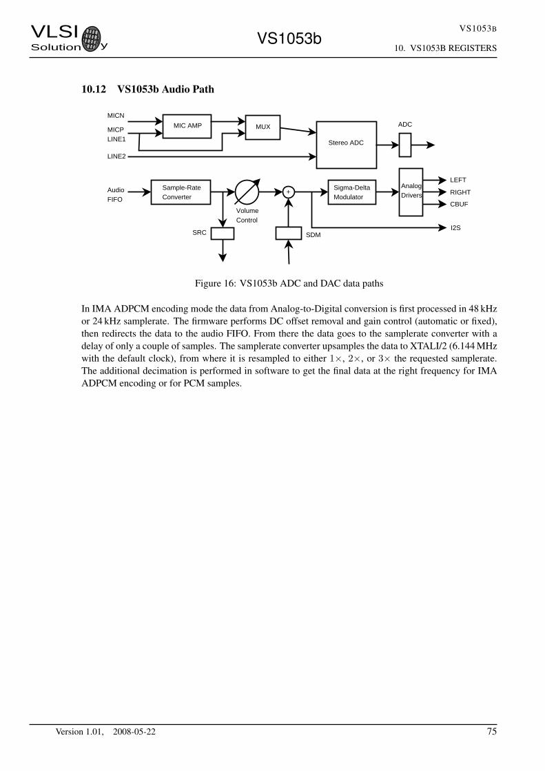
VLSISolution y VS1053b
VS1053B
10. VS1053B REGISTERS
10.12 VS1053b Audio Path
MIC AMP MUX
Stereo ADC
MICN
MICPLINE1
LINE2
Sample-RateConverter
AudioFIFO
+
VolumeControl
SDMSRC
Sigma-DeltaModulator
AnalogDrivers
ADC
LEFT
RIGHT
CBUF
I2S
Figure 16: VS1053b ADC and DAC data paths
In IMA ADPCM encoding mode the data from Analog-to-Digital conversion is first processed in 48 kHzor 24 kHz samplerate. The firmware performs DC offset removal and gain control (automatic or fixed),then redirects the data to the audio FIFO. From there the data goes to the samplerate converter with adelay of only a couple of samples. The samplerate converter upsamples the data to XTALI/2 (6.144 MHzwith the default clock), from where it is resampled to either 1×, 2×, or 3× the requested samplerate.The additional decimation is performed in software to get the final data at the right frequency for IMAADPCM encoding or for PCM samples.
Version 1.01, 2008-05-22 75

VLSISolution y VS1053b
VS1053B
10. VS1053B REGISTERS
10.13 I2S DAC Interface
The I2S Interface makes it possible to attach an external DAC to the system.
Note: in VS1053b the I2S pins share different GPIO pins than in VS1033 to be able to use SPI boot andI2S in the same application.
10.13.1 Registers
I2S registers, prefix I2SReg Type Reset Abbrev Description
0xC040 r/w 0 CONFIG[3:0] I2S configuration
10.13.2 Configuration I2S CONFIG
I2S CONFIG BitsName Bits DescriptionI2S CF MCLK ENA 3 Enables the MCLK output (12.288 MHz)I2S CF ENA 2 Enables I2S, otherwise pins are GPIOI2S CF SRATE 1:0 I2S rate, ”10” = 192, ”01” = 96, ”00” = 48 kHz
I2S CF ENA enables the I2S interface. After reset the interface is disabled and the pins are used forGPIO.
I2S CF MCLK ENA enables the MCLK output. The frequency is either directly the input clock (nom-inal 12.288 MHz), or half the input clock when mode register bit SM CLK RANGE is set to 1 (24-26 MHz input clock).
I2S CF SRATE controls the output samplerate. When set to 48 kHz, SCLK is MCLK divided by 8,when 96 kHz SCLK is MCLK divided by 4, and when 192 kHz SCLK is MCLK divided by 2.
MCLK
SDATA
SCLK
LROUT
MSB LSB MSB
Left Channel Word Right Channel Word
Figure 17: I2S Interface, 192 kHz.
To enable I2S first write 0xc017 to SCI WRAMADDR and 0xf3 to SCI WRAM, then write 0xc040 toSCI WRAMADDR and 0x0c to SCI WRAM.
See application notes for more information.
Version 1.01, 2008-05-22 76

VLSISolution y VS1053b
VS1053B
11. VS1053 VERSION CHANGES
11 VS1053 Version Changes
This chapter describes the lastest and most important changes done to VS1053.
11.1 Changes Between VS1033c and VS1053a/b Firmware, 2007-03-08
Completely new or major changes:
• I2S pins are now in GPIO4-GPIO7 and do not overlap with SPI boot pins.
• No software reset required between files when used correctly.
• Ogg Vorbis decoding added. Non-fatal ogg or vorbis decode errors cause automatic resync.This allows easy rewind and fast forward. Decoding ends if the ”last frame” flag is reached orSM CANCEL is set.
• HE-AAC v2 Level 3 decoding added. It is possible to disable PS and SBR processing and controlthe upsampling modes through parametric x.control1.
• Like the WMA decoder, the AAC decoder uses the clock adder (see SCI CLOCKF) if it needsmore clock to decode the file. HE-AAC features are dropped one by one, if the file can not bedecoded correctly even with the highest allowed clock. Parametric stereo is the first feature tobe dropped, then downsampled mode is used, and as the final resort Spectral Band Replication isdisabled. Features are automatically restored for the next file.
• Completely new volume control with zero-cross detection prevents pops when volume is changed.
• Audio FIFO underrun detection (with slow fade to zero) instead of looping the audio buffer content.
• Average bitrate calculation (byteRate) for all codecs.
• All codecs support fast play mode with selectable speeds for the best-quality fast forward opera-tion. Fast play also advances DECODE TIME faster.
• WMA and Ogg Vorbis provide an absolute decode position in milliseconds.
• When SM CANCEL is detected, the firmware also discards the stream buffer contents.
• Bit SCIST DO NOT JUMP in SCI STATUS is ’1’ when jumps in the file should not be done:during header processing and with Midi files.
• IMA ADPCM encode now supports stereo encoding and selectable samplerate.
Other changes or additions:
• Delayed volume and bass/treble control calculation reduces the time the corresponding SCI oper-ations take. This delayed handling and the new volume control hardware prevents audio samplesfrom being missed during volume change.
• SCI DECODE TIME only cleared at hardware and software reset to allow files to be played back-to-back or looped.
• Read and write to YRAM at 0xe000..0xffff added to SCI WRAMADDR/SCI WRAM.
• The resync parameter (parametric x.resync) is set to 32767 after reset to allow inifinite resyn-chronization attempts (or until SM CANCEL is set). Old operation can be restored by writing 0to resync after reset.
Version 1.01, 2008-05-22 77

VLSISolution y VS1053b
VS1053B
11. VS1053 VERSION CHANGES
• WMA,AAC: more robust resync.
• WMA,AAC: If resync is performed, broadcast mode is automatically activated. The broadcastmode disables file size checking, and decoding continues until SM CANCEL is set or reset isperformed.
• Treble control fixed (volume change could cause bad artefacts).
• MPEG Layer I mono fixed.
• MPEG Layer II half-rate decoding fixed (frame size was calculated wrong).
• MPEG Layer II accuracy problem fixed, invalid grouped values set to 0.
• WAV parser now skips unknown RIFF chunks.
• IMA ADPCM: Maximum blocksize is now 4096 bytes (4088 samples stereo, 8184 mono). Thus,now also plays 44100Hz stereo.
• Rt-midi: starts if in reset GPIO0=’0’, GPIO1=’1’, GPIO2&3 give earSpeaker setup.
• NewSinTest() and NewSinSweep() added (AIADDR = 0x4020/0x4022) AICTRL0 and AICTRL1set sin frequency for left/right.
• Clears memory before SPI boot and not in InitHardware().
Known quirks, bugs, or features in VS1053b:
• Setting volume clears SS REFERENCE SEL and SS AD CLOCK bits. See Chapter 8.7.2.
• Software reset clears GPIO DDR, also affects I2S pins.
• Ogg Vorbis occasionally overflows in windowing causing a small glitch to audio. Patch available.
• IMA ADPCM encoding requires short patch to start. Patch available in Chapter 9.8.1.
Version 1.01, 2008-05-22 78

VLSISolution y VS1053b
VS1053B
12. DOCUMENT VERSION CHANGES
12 Document Version Changes
This chapter describes the most important changes to this document.
Version 1.01 for VS1053b, 2008-05-22
• Added IMA ADPCM patch to Chapter 9.8.1.
Version 1.0 for VS1053b, 2008-05-12
• Production version, removed “PRELIMINARY” tag.
• Update values to tables in Chapter 4.
• Changed minimum temperature back to -30C.
• Changed maximum SCI Read speed to CLKI/7.
Version 0.5 for VS1053b, 2007-12-03
• Ogg Vorbis recording now documented in Chapter 9.7.
• Added stereo ADPCM recording and an example to Chapter 9.8.
• Added WAV PCM header example to Chapter 9.6.
• Simplified LQFP-48 Typical Connection Diagram (Chapter 6) by removing one of the images.
Version 0.4 for VS1053b, 2007-09-06
• First published version.
• Completely rewritten Chapter 9.5: Operation / Play and Decode. New designs should be based onthis new version.
• Updated Image 3: Typical Connection Diagram Using LQFP-48.
• Rename SM OUTOFWAV SM CANCEL.
• Many minor changes like typo corrections.
Version 0.3 for VS1053a, 2007-01-16
• I2S pins are now in GPIO4-GPIO7, they no longer overlap with GPIO0 and GPIO1.
• Extra parameter structure updated (version 3), location changed to X:0x1e00.
Version 1.01, 2008-05-22 79

VLSISolution y VS1053b
VS1053B
13. CONTACT INFORMATION
13 Contact Information
VLSI Solution OyEntrance G, 2nd floor
Hermiankatu 8FIN-33720 Tampere
FINLAND
Fax: +358-3-3140-8288Phone: +358-3-3140-8200
Email: [email protected]: http://www.vlsi.fi/
Version 1.01, 2008-05-22 80

PENNSYLVANIA STATE UNIVERSITY
Sumo Bot ME 445 Microcomputer Interfacing
Anthony Burt Eric Skibba
5/2/2013

1
Table of Contents Introduction .................................................................................................................................................. 2
Robot Overview ........................................................................................................................................ 2
Control Strategy ............................................................................................................................................ 2
Overview ................................................................................................................................................... 2
Component Integration ............................................................................................................................ 3
IR Sensor ............................................................................................................................................... 3
Front Optical Sensor ............................................................................................................................. 3
Servo with Flipper ................................................................................................................................. 3
Right and Left Optical Sensors .............................................................................................................. 4
Calibration ..................................................................................................................................................... 4
Performance During Battle ........................................................................................................................... 7
Appendices .................................................................................................................................................... 8
Appendix A: Control Strategy Flow Chart ................................................................................................. 8
Appendix B: MultiMap Function From Arduino Play Ground ................................................................... 9
Appendix C: Sumo Bot Control Program ................................................................................................... 9
Appendix D: Sources ............................................................................................................................... 17
2
Introduction
Robot Overview Each of the three teams participating in the Sumo Bot competition were provided with an Arduino Uno and a Zumo Shield attached to a Zumo chassis. The Zumo Shield and chassis provide for an easy and convenient means for attaching the Arduino Uno to a sturdy chassis with wheels connected to controllable servos. Other components that we added to our robot include three Sharp optical distance sensors, a servo, and the competition required Pololu IR sensor. The basic concept for the robot was to control it to push, flip, and avoid being pushed by the other robots.
Control Strategy
Overview Our strategy for controlling the robot begins with finding the opponent bot with the IR sensor. The bot would then orient itself to point towards the opponent and go forward. The IR sensor is continuously reading the other bots position so that our bot can continue to orient itself to face the opponent. Once the opponent’s bot is in front of ours, our bot would move forward until the front distance sensor read a distance of less than 7cm. Once this value was read the servo was actuated in an attempt to flip the other bot. After the servo lifted the flipper, our bot moved backwards to reposition itself to face the opponent and attempt to flip the opponent again. This was also done to prevent the flipper from being placed down on the opponent which would in turn likely flip our bot. If a situation arose that a wall was within 10cm of our bot to the right or left one of the two side sensors would read this and our bot would back up and turn the opposite direction. The detection of a wall was differentiated from the detection of the opponent by use of the IR sensor. Our bot only executed this maneuver to get away from a wall if the IR sensor detected the opponent in another direction. This maneuver was also used to escape the situation of being pushed from the side into a wall. A flow chart of our control strategy can be found in Appendix A: Control Strategy Flow Chart.

3
Component Integration
Figure 1: Component Location
IR Sensor
As required by the competition, the IR sensor was mounted 4” above the Arduino and was the highest point of the bot. This component communicated with the IR sensor on the opponent’s bot and was used for simple detection of a rough relative location of the opponent. This reading was used along with the other sensors to preform specific operations. For instance if the sensor that triggers the servo saw an object close to the bot, the servo would only actuate if the IR detector sensed that the opponent was in front of our bot.
Front Optical Sensor
The front optical sensor had a range that we tested of 4 to 40cm. This component was used to simply detect the distance to the opponent and triggered the servo when it saw an object was 7cm in front of the sensor.
Servo with Flipper
The servo mounted on the front of the bot was directly coupled with a steel flipper. The purpose of these two components was to lift the opponent’s bot with intention of turning them over. When the front optical sensor detected the opponent within 7cm of the sensor and the IR sensor detected the opponent in front of our bot, the servo was enabled.

4
Right and Left Optical Sensors
The right and left optical sensors had a tested range of 6 to 80cm. These two sensors were used in tandem to detect the situation of our opponent’s bot pushing ours from the side. When the two sensors detected objects within 10cm on both sides, our bot executed an escape maneuver. The escape maneuver had our bot move backwards then turn. The direction that the bot turned was determined by the two side sensors. Whichever sensor still detected an object within 10cm (i.e. the wall) the bot turned the opposite direction.
Calibration Both of the SHARP distance sensors that the team used output an analog voltage that can be scaled with distance away from the sensor. Unfortunately this relationship between output voltage and distance is non-linear. In order to obtain the relationship between the distance and the output voltage of the sensor the group had to set up a bench test to obtain a relationship between output voltage and distance away from the sensor. Figure 2, shown below is the test setup used for both of the SHARP distance sensors.
Figure 2: Test Setup Used for Calibrating the Distance Sensors
The sensor was placed at one end of a ruler and then a large piece of cardboard was moved away from the sensor in increments of 2cm. The output from sensor was then recorded. Figure 3-6 show the data collected along with the data from the corresponding data sheet. By comparing the data from the groups testing to the data from the corresponding data sheet one can see that both sets of data are fairly close this validated the group’s ability to use this data to calibrate the distance sensors.

5
Figure 3: Voltage Vs. Distance Data Recorded With The SHARP 2D120X Distance Sensor
Figure 4: Voltage Vs. Distance Data From The SHARP 2D120X Distance Sensor Data Sheet

6
Figure 5: Voltage Vs. Distance Data Recorded With The SHARP 2Y0A21 Distance Sensor
Figure 6:Voltage Vs. Distance Data From The SHARP 2Y0A21 Distance Sensor Data Sheet

7
Since the data from the sensors is non linear, the group needed to find another way relate the output voltage to the distance of an object from the sensor. After some searching on the Arduino Playground the group found a function called multiMap, this function takes two arrays, one with distances that were used for the measurement, and one with the corresponding analogRead() values. This function will then linearly interpolate in-between the data points to return the distance from the sensor (Tillaart, 2011). The code for this function can be found in the appendix.
Performance During Battle Complications with the optical sensors caused our bot to perform in an undesirable manner. For reasons that we have yet to determine, the three optical sensors were not reading distances properly. This caused the servo to not function, as the Arduino never received the proper distance readings from the front optical sensor to trigger the servo. Although we were not getting proper distance readings from the side optical sensors, our bot still followed our control strategy properly. The readings from the two side sensors were similar, causing the robot to think that it was being pushed into a wall sideways by the opponent. The bot then backed up and turned in the same fashion as the escape maneuver that we had programmed. In conclusion, even though proper distances were not read by the optical sensors, and the bot performed very poorly during battle, our control strategy was followed exactly how we had intended it to.

8
Appendices
Appendix A: Control Strategy Flow Chart
Start
Look For Other Robot
Is North LOW?
Go Forward
Is Front Distance <=7cm?
Flip
Go backwards
Is Right Distance <=10cm?
Go backwards
Turn Left
Go Forward
Is Left Distance <=10cm?
Go backwards
Turn Right
Go Forward
NO
YES
YES
NO
NO
Yes
NO
Yes

9
Appendix B: MultiMap Function From Arduino Play Ground
int multiMap(int val, int* _in, int* _out, uint8_t size)
// take care the value is within range
// val = constrain(val, _in[0], _in[size-1]);
if (val <= _in[0]) return _out[0];
if (val >= _in[size-1]) return _out[size-1];
// search right interval
uint8_t pos = 1; // _in[0] allready tested
while(val > _in[pos]) pos++;
// this will handle all exact "points" in the _in array
if (val == _in[pos]) return _out[pos];
// interpolate in the right segment for the rest
return map(val, _in[pos-1], _in[pos], _out[pos-1], _out[pos]);
Appendix C: Sumo Bot Control Program //Anthony M. Burt & Eric Skibba
//ME 445
//Sumo Bot
//Program will control our Sumo Bot
#include <Servo.h> //includes servo library
//Sets up variables that will serve as pin assignment for
//motor control
int rightdir=7; //Direction pin for right motor
int leftdir=8; //Direction pin for left motor
int rightsp=9; //Speed control pin for right motor
int leftsp=10; //Speed control pin for left motor
//Sets up variables that will serve as pin assignment for
//IR beacon outputs
int north=3; //Digital pin for "North" direction
int east=4; //Digital pin for "East" direction

10
int south=5; //Digital pin for "South" direction
int west=11; //Digital pin for "West" direction
//IR beacon inputs
int iren=12; //IR beacon enable pin
int irpwr=13; //IR beacon power pin
//Sets up variables that will serve as pin
//assignment for distance sensors
int frontsens=A5; //Analog input pin for front sensor
int rightsens=A3; //Analog input pin for right side sensor
int leftsens=A4; //Analog input pin for left side sensor
//Sets up variables that will hold the analogRead() values
//from the distance sensors
int frontval; //Analog values from front sensor
int rightval; //Analog values from right side sensor
int leftval; //Analog values from left side sensor
//Sets up variables that will hold the distance values
//from the distance sensors
int frontdis; //variable for distance from front sensor
int rightdis; //variable for distance from right sensor
int leftdis; //variable for distance from left sensor
Servo myservo;//create servo object to control flipper servo
//calibrated distance sensor - SHARP 2Y0A21 (we use the integer outputs from the analog pins to allow
for faster performance)
//2Yout[] holds values wanted in cm
int Yout[] =
80,74,70,64,58,56,54,52,50,48,46,44,42,40,38,36,34,32,30,28,26,24,22,20,18,16,14,12,10,8,6;
//2Yin holds measured analogRead()values for the defined distances
int
Yin[]=70,74,78,86,95,99,103,107,110,114,122,126,130,138,146,153,161,169,181,192,208,224,239,262,
287,321,367,421,501,628,633;
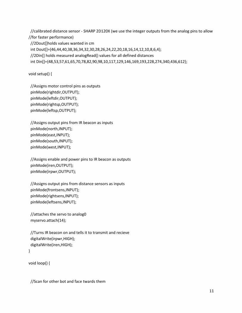
11
//calibrated distance sensor - SHARP 2D120X (we use the integer outputs from the analog pins to allow
//for faster performance)
//2Dout[]holds values wanted in cm
int Dout[]=46,44,40,38,36,34,32,30,28,26,24,22,20,18,16,14,12,10,8,6,4;
//2Din[] holds measured analogRead() values for all defined distances
int Din[]=48,53,57,61,65,70,78,82,90,98,10,117,129,146,169,193,228,274,340,436,612;
void setup()
//Assigns motor control pins as outputs
pinMode(rightdir,OUTPUT);
pinMode(leftdir,OUTPUT);
pinMode(rightsp,OUTPUT);
pinMode(leftsp,OUTPUT);
//Assigns output pins from IR beacon as inputs
pinMode(north,INPUT);
pinMode(east,INPUT);
pinMode(south,INPUT);
pinMode(west,INPUT);
//Assigns enable and power pins to IR beacon as outputs
pinMode(iren,OUTPUT);
pinMode(irpwr,OUTPUT);
//Assigns output pins from distance sensors as inputs
pinMode(frontsens,INPUT);
pinMode(rightsens,INPUT);
pinMode(leftsens,INPUT);
//attaches the servo to analog0
myservo.attach(14);
//Turns IR beacon on and tells it to transmit and recieve
digitalWrite(irpwr,HIGH);
digitalWrite(iren,HIGH);
void loop()
//Scan for other bot and face twards them

12
scan(north,east,south,west,rightdir,leftdir,rightsp,leftsp);
//Reads in analog data from the distance sensor
frontval=analogRead(frontsens);
rightval=analogRead(rightsens);
leftval=analogRead(leftsens);
//Applies the multimap function from arduino playground which will linearly interpolate
//to get distances
frontdis=multiMap(frontval,Din,Dout,21);
rightdis=multiMap(rightval,Yin,Yout,31);
leftdis=multiMap(leftval,Yin,Yout,31);
//reads in the current status of north directioin pin from th IR beacon
digitalRead(north);
//while loop to start as long as the enemy bot is infront of ours (North==Low)
while(north==LOW)
//goes forward because the enemy bot is infront of our bot
forward(rightdir,leftdir,rightsp,leftsp,255);
//Reads in analog data from the distance sensor
frontval=analogRead(frontsens);
rightval=analogRead(rightsens);
leftval=analogRead(leftsens);
//Applies the multimap function from arduino playground which will linearly interpolate
//to get distances
frontdis=multiMap(frontval,Din,Dout,21);
rightdis=multiMap(rightval,Yin,Yout,31);
leftdis=multiMap(leftval,Yin,2out,31);
//Starts if statement for when enemy bot is close enough for flipper to be used
if (frontdis<=7)
//Stops robot
kill(rightsp,leftsp);
//moves servo 30deg to flip enemy
myservo.write(30);

13
//waits 500ms
delay(500);
//sends robot backwards
backwards(rightdir,leftdir,rightsp,leftsp,255);
//waits 300ms
delay(300);
//returns servo to original position
myservo.write(135);
//starts if statement for when there is a side obsitcle close to
//the robot such as a wall or enemy within 10cm of bot
if (rightdis<=10)
//sends robot backwards
backwards(rightdir,leftdir,rightsp,leftsp,255);
//waits 500ms
delay(500);
//robot turns left because the obsticle is to the right of bot
left(rightdir,leftdir,rightsp,leftsp,255);
//waits 200ms
delay(200);
//moves robot forward
forward(rightdir,leftdir,rightsp,leftsp,255);
//waits 1000ms or 1sec
delay(1000);
//stops robot
kill(rightsp,leftsp);
//starts if statement for when there is a side obsitcle close to
//the robot such as a wall or enemy within 10cm of bot

14
if (leftdis<=10)
//sends robot backwards
backwards(rightdir,leftdir,rightsp,leftsp,255);
//waits 500ms
delay(500);
//turns robot to the right because obsticle is on the left of the bot
right(rightdir,leftdir,rightsp,leftsp,255);
//waits 200ms
delay(200);
//moves robot forward
forward(rightdir,leftdir,rightsp,leftsp,255);
//waits 1000ms or 1sec
delay(1000);
//stops robot
kill(rightsp,leftsp);
//reads in current status of the "North" to check for changes
digitalRead(north);
//function for scanning (looking for enemy bot
void scan(int north, int east, int south, int west, int rightdir, int leftdir, int rightsp, int leftsp)
//sets up inputs from IR beacon
pinMode(north,INPUT);
pinMode(east,INPUT);
pinMode(south,INPUT);
pinMode(west,INPUT);
//sests up outputs to control robot speed and direction
pinMode(rightdir,OUTPUT);
pinMode(leftdir,OUTPUT);
pinMode(rightsp,OUTPUT);

15
pinMode(leftsp,OUTPUT);
//moves robot right
right(rightdir,leftdir,rightsp,leftsp,150);
//reads in current status of "North" pin
digitalRead(north);
//starts while loop to run while "North" pin is High meaning that the
//enemy is not infront of the bot
while(north==HIGH)
//moves robot right
right(rightdir,leftdir,rightsp,leftsp,150);
//reads in current status of "North" pin to look for changes
digitalRead(north);
//When while loop is terminated it means that our bot is pointing
//straight at the enemy so the bot will stop
kill(rightsp,leftsp);
//function for moving bot forward
void forward(int rightdir,int leftdir,int rightsp,int leftsp,int sp)
//sets pins for motor control as outputs
pinMode(rightdir,OUTPUT);
pinMode(leftdir,OUTPUT);
pinMode(rightsp,OUTPUT);
pinMode(leftsp,OUTPUT);
digitalWrite(rightdir,LOW); //sets direction of right motor
digitalWrite(leftdir,LOW); //sets direction of left motor(same as right motor)
analogWrite(rightsp,sp); //sets speed of right motor
analogWrite(leftsp,sp); //sets speed of left motor(same as right motor)
//function for moving bot backwards
void backwards(int rightdir,int leftdir,int rightsp,int leftsp,int sp)

16
//sets pins for motor control as outputs
pinMode(rightdir,OUTPUT);
pinMode(leftdir,OUTPUT);
pinMode(rightsp,OUTPUT);
pinMode(leftsp,OUTPUT);
digitalWrite(rightdir,HIGH); //sets direction of right motor
digitalWrite(leftdir,HIGH); //sets direction of left motor (same as right motor)
analogWrite(rightsp,sp); //sets speed of right motor
analogWrite(leftsp,sp); //sets speed of left motor(same as right motor)
//function for turning bot to the right
void right(int rightdir, int leftdir, int rightsp, int leftsp, int sp)
//sets pins for motor control as outputs
pinMode(rightdir,OUTPUT);
pinMode(leftdir,OUTPUT);
pinMode(rightsp,OUTPUT);
pinMode(leftsp,OUTPUT);
digitalWrite(rightdir,HIGH); //sets direction of right motor
digitalWrite(leftdir,LOW); //sets direction of left motor
//(opposite of right motor for tighter turn)
analogWrite(rightsp,sp); //sets speed of right motor
analogWrite(leftsp,sp); //sets speed of left motor (same as right motor)
//function for turning bot left
void left(int rightdir, int leftdir, int rightsp, int leftsp,int sp)
//sets pins for motor control as outputs
pinMode(rightdir,OUTPUT);
pinMode(leftdir,OUTPUT);
pinMode(rightsp,OUTPUT);
pinMode(leftsp,OUTPUT);
digitalWrite(rightdir,LOW); //sets direction of right motor
digitalWrite(leftdir,HIGH); //sets direction of left motor
//(opposite of right motor for tighter turning)
analogWrite(rightsp,sp); //sets speed of right motor
analogWrite(leftsp,sp); //sets speed of left motor (same as right motor)

17
//function for stopping bot
void kill(int rightsp, int leftsp)
//sets pins for motor control as ouputs (we only care about speed pins for this)
pinMode(rightsp,OUTPUT);
pinMode(leftsp,OUTPUT);
analogWrite(rightsp,0); //sets speed of right motor to 0
analogWrite(leftsp,0); //sets speed of left motor to 0
//function multiMap to get distance measurements from distance sensors
//Source: Arduino Playground
//Author: Robert Tillaart
//Website: http://playground.arduino.cc/Main/MultiMap
int multiMap(int val, int* _in, int* _out, uint8_t size)
// take care the value is within range
// val = constrain(val, _in[0], _in[size-1]);
if (val <= _in[0]) return _out[0];
if (val >= _in[size-1]) return _out[size-1];
// search right interval
uint8_t pos = 1; // _in[0] allready tested
while(val > _in[pos]) pos++;
// this will handle all exact "points" in the _in array
if (val == _in[pos]) return _out[pos];
// interpolate in the right segment for the rest
return map(val, _in[pos-1], _in[pos], _out[pos-1], _out[pos]);
Appendix D: Sources
Tillaart, R. (2011, March 23). MultiMap. Retrieved May 2, 2013, from Arduino Playground:
http://playground.arduino.cc/Main/MultiMap
ME 445 Final Project Report Sumo Battle Bot
Chris Carrero Tyler Holp Lauren Williams
May 2, 2013

ME 445 Final Project Carrero, Holp, Williams
2
Table of Contents Project Overview ...................................................................................................................................... 3
Retrofitting and Customization ............................................................................................................. 4
Additional Sensors ............................................................................................................................... 5
Defensive and Offensive Design ..................................................................................................... 5
Coding .......................................................................................................................................................... 6
Results and Discussion ............................................................................................................................ 7
Conclusion .................................................................................................................................................. 7
Bibliography ............................................................................................................................................... 8
Appendix ..................................................................................................................................................... 8

ME 445 Final Project Carrero, Holp, Williams
3
Project Overview
Our choice for the final project in ME 445 was to retrofit a stock sumo-bot with the goal
of winning a battle-bot competition against other groups. As a novice group in the
knowledge of electronics and mechatronics, we knew this would be a challenging project
to overcome.
The foundation for the project was Pololu’s Ardunio-controlled Zumo Robot (Zumo),
which each group was given to retrofit and customize. Each group could use servos,
sensors, or any mechatronic design with the stipulation that it did not permanently
damage the Zumo.
Following testing and tweaking of each design, the groups battled off in a closed-arena to
see which design was victorious. The competition was set up so each will fight the other
bots individually for 3 minutes; with a championship match for 5 minutes. The scoring of
the competition for each of the matches was as follows: 3 points for flipping the other
robot over, 1 point if the other robot stands back up within 10 seconds, 1 point for
pushing the other robot into the wall, and -1 point for running into the wall ourselves.

ME 445 Final Project Carrero, Holp, Williams
4
Retrofitting and Customization
As mentioned before the foundation for the project was Pololu’s Zumo. The Zumo is a
robot specifically designed to work in conjunction with the Arduino interfaces.
Engineering into the Zumo are many different tools such as accelerometers, buzzers, and
a compass that can be utilized for any design. The Zumo is equipped with four 2200 mAh
Nickel-metal hydride batteries that power the micro-gear motors, Arduino, and any other
electrical devices.
The Arduino we used for our project was the class standard Arduino UNO. As can be
seen in Figure 1, the Zumo is equipped with SIP Headers which matches with the Uno
sockets. This enables the Arduino to control the Zumo but also expand the terminals,
giving the possibility of more connections.
As part of the competition, each group was given a Pololu Infrared Beacon Transceiver
seen in Figure 2. This IR beacon allows each Zumo to locate one-another by transmitting
infrared light to and receiving infrared light from the other bot. Each beacon is equipped
with four IR receivers which are denoted North, East,
South, and West. When the sensor detects the
direction of the other Zumo it illuminates an LED in
the direction where it thinks it is. To ensure
uniformity, an agreed design requirement for all of the
groups was to mount this sensor 4 inches above the
Zumo. While this given sensors was very helpful to
our project, we decided to buy a few more sensors to
give our bot the competitive edge.
Figure 1 - Pololu Zumo Robot
Figure 2 - Pololu IR Beacon Transceiver
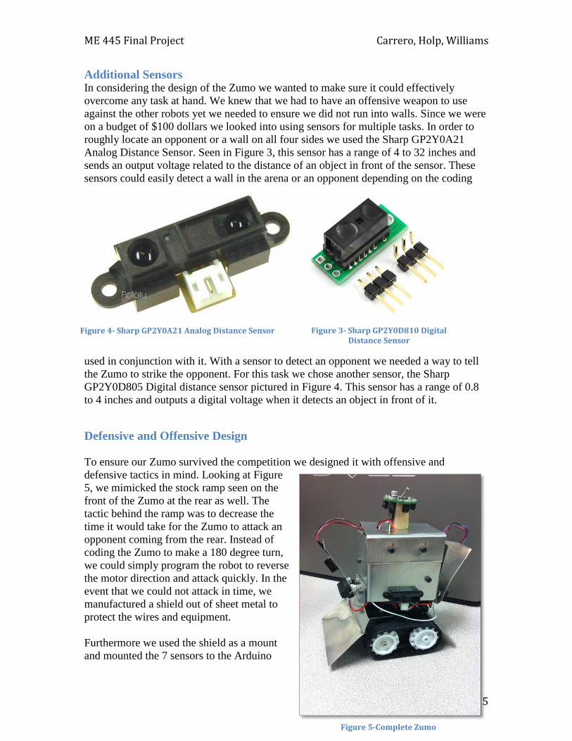
ME 445 Final Project Carrero, Holp, Williams
5
Additional Sensors In considering the design of the Zumo we wanted to make sure it could effectively
overcome any task at hand. We knew that we had to have an offensive weapon to use
against the other robots yet we needed to ensure we did not run into walls. Since we were
on a budget of $100 dollars we looked into using sensors for multiple tasks. In order to
roughly locate an opponent or a wall on all four sides we used the Sharp GP2Y0A21
Analog Distance Sensor. Seen in Figure 3, this sensor has a range of 4 to 32 inches and
sends an output voltage related to the distance of an object in front of the sensor. These
sensors could easily detect a wall in the arena or an opponent depending on the coding
used in conjunction with it. With a sensor to detect an opponent we needed a way to tell
the Zumo to strike the opponent. For this task we chose another sensor, the Sharp
GP2Y0D805 Digital distance sensor pictured in Figure 4. This sensor has a range of 0.8
to 4 inches and outputs a digital voltage when it detects an object in front of it.
Defensive and Offensive Design
To ensure our Zumo survived the competition we designed it with offensive and
defensive tactics in mind. Looking at Figure
5, we mimicked the stock ramp seen on the
front of the Zumo at the rear as well. The
tactic behind the ramp was to decrease the
time it would take for the Zumo to attack an
opponent coming from the rear. Instead of
coding the Zumo to make a 180 degree turn,
we could simply program the robot to reverse
the motor direction and attack quickly. In the
event that we could not attack in time, we
manufactured a shield out of sheet metal to
protect the wires and equipment.
Furthermore we used the shield as a mount
and mounted the 7 sensors to the Arduino
Figure 4- Sharp GP2Y0A21 Analog Distance Sensor Figure 3- Sharp GP2Y0D810 Digital Distance Sensor
Figure 5-Complete Zumo
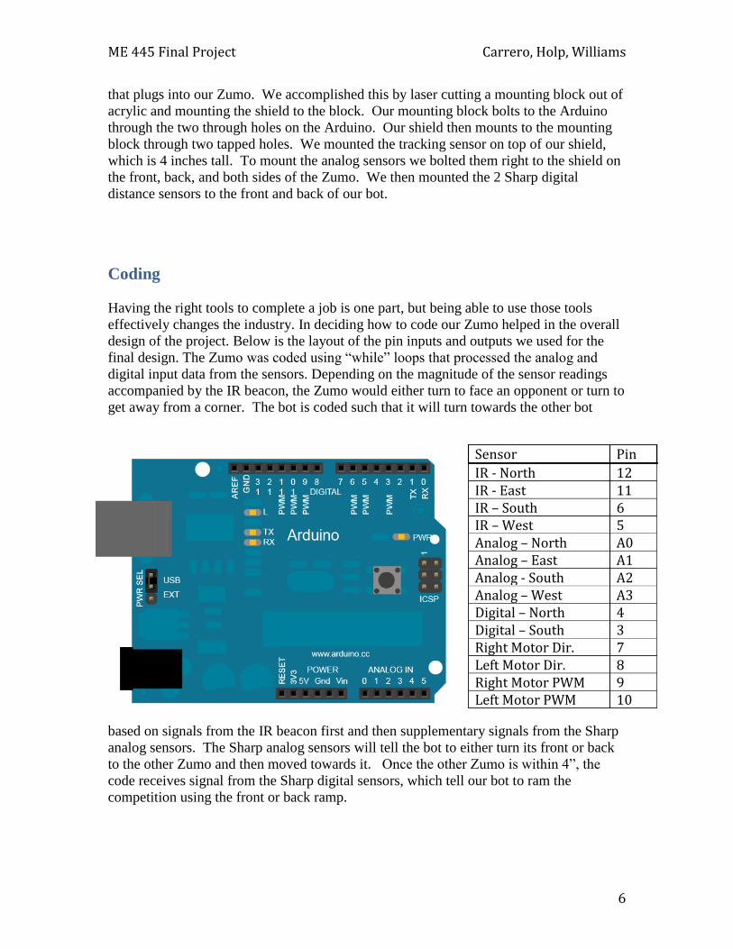
ME 445 Final Project Carrero, Holp, Williams
6
that plugs into our Zumo. We accomplished this by laser cutting a mounting block out of
acrylic and mounting the shield to the block. Our mounting block bolts to the Arduino
through the two through holes on the Arduino. Our shield then mounts to the mounting
block through two tapped holes. We mounted the tracking sensor on top of our shield,
which is 4 inches tall. To mount the analog sensors we bolted them right to the shield on
the front, back, and both sides of the Zumo. We then mounted the 2 Sharp digital
distance sensors to the front and back of our bot.
Coding
Having the right tools to complete a job is one part, but being able to use those tools
effectively changes the industry. In deciding how to code our Zumo helped in the overall
design of the project. Below is the layout of the pin inputs and outputs we used for the
final design. The Zumo was coded using “while” loops that processed the analog and
digital input data from the sensors. Depending on the magnitude of the sensor readings
accompanied by the IR beacon, the Zumo would either turn to face an opponent or turn to
get away from a corner. The bot is coded such that it will turn towards the other bot
based on signals from the IR beacon first and then supplementary signals from the Sharp
analog sensors. The Sharp analog sensors will tell the bot to either turn its front or back
to the other Zumo and then moved towards it. Once the other Zumo is within 4”, the
code receives signal from the Sharp digital sensors, which tell our bot to ram the
competition using the front or back ramp.
Sensor Pin
IR - North 12 IR - East 11 IR – South 6 IR – West 5 Analog – North A0 Analog – East A1 Analog - South A2 Analog – West A3 Digital – North 4 Digital – South 3 Right Motor Dir. 7 Left Motor Dir. 8 Right Motor PWM 9 Left Motor PWM 10

ME 445 Final Project Carrero, Holp, Williams
7
Results and Discussion In the first match of our competition, we battled Group 3’s Zumo bot for 3 minutes. We
scored 2 points in the match by pushing their bot into the wall and they scored -2 points
for running into the wall on their own.
In the second match of our competition, we battled Group 13’s Zumo bot. We won this
second match by a score of 6 to -2. Once again, we scored a number of points by pushing
the other team’s bot into the wall. We also sat back and let them run into the wall so they
would accumulate negative points.
In the championship match, we faced Group 3’s Zumo bot again. We lost the
championship match by a score of 3 to -1. We were unable to push their bot into the wall
because they were too heavy after some modifications that they made. If we had more
power, we would have been able to push them better and possible win the tournament.
We were able to battle effectively by coding our Zumo bot to remain patient and wait for
our opponent to come into our close range. Once the IR beacon and one of the Sharp
analog distance sensors both picked up the motion of the other bot, our Zumo bot turned
one of its ramps towards the other bot and pushed full speed forward. This technique was
effective because we were able to scored our points by pushing the other bot into the
wall.
Some improvements could be made to our Zumo bot to make it better for battle. After
our first match, we noticed that our Zumo bot was turning slowly to line its ramp up with
the other bot. To remedy this problem, we increased the turning speed of our Zumo bot
in our code. We also noticed that our bot would jump back and forth if the other bot was
in between two of our four Sharp analog sensors. We could have remedied this problem
by taking the average of the analog sensors and telling our bot to turn towards that
direction. Additionally, we noticed that our two Sharp digital sensors were pointed too
directly toward the ground right in front of the two ramps. After the first match, we
increased the range that the digital sensors could read the other bots in by bending their
part of the shield up, making them point more straight forward.
Conclusion For our final project, we were able to customize and retrofit a Pololu Zumo bot to
effectively win in battles against the other Zumo bots in our class. We added another
ramp to the back end of our bot, a protective shield, and 6 Sharp distance sensors (4
analog for long distance, 2 digital for short distances). We coded the bot to wait for its
opponent to approach before making its move. Our Zumo bot quickly turns if the sensors
on its side detect the other bot, and aligns itself so it is facing the opponent. If the sensors
on the front or back detect the other bot, our Zumo bot moves quickly straight ahead to
hopefully run the other bot into the wall. Although we did not win the competition, we
learned a created an effective Zumo bot and learned a lot about its mechatronics.

ME 445 Final Project Carrero, Holp, Williams
8
Bibliography The following data sheets can be found attached to the end of this report.
Sharp analog sensor data sheet
Sharp digital sensor data sheet
Appendix
#include <ZumoMotors.h>
ZumoMotors motors;
int compnorth = 12;
int compeast = 11;
int compsouth = 6;
int compwest = 5;
int engagefront = 4;
int engagerear = 3;
int time = 0;
int straightspeed = 300;
int turn = 250;
int hide = 2;
int cornerprox = 400;
int opponentprox = 350;
void setup()
Serial.begin(9600);
pinMode(compnorth, INPUT);
pinMode(compeast, INPUT);
pinMode(compsouth, INPUT);
pinMode(compwest, INPUT);
pinMode(engagefront, INPUT);
pinMode(engagerear, INPUT);
void loop()
int north = digitalRead(compnorth);
Serial.print("Compass North : ");
Serial.print(north);
int east = digitalRead(compeast);
Serial.print(" Compass East : ");
Serial.print(east);
int west = digitalRead(compwest);
Serial.print(" Compass West : ");
Serial.print(west);

ME 445 Final Project Carrero, Holp, Williams
9
int south = digitalRead(compsouth);
Serial.print(" Compass South : ");
Serial.print(south);
int front = digitalRead(engagefront);
Serial.print(" Engage Front : ");
Serial.print(front);
int rear = digitalRead(engagerear);
Serial.print("Engage Rear : ");
Serial.print(rear);
int northsens = analogRead(A0);
Serial.print(" North Sensor : ");
Serial.print(northsens);
int eastsens = analogRead(A1);
Serial.print(" East Sensor : ");
Serial.print(eastsens);
int southsens = analogRead(A2);
Serial.print(" South Sensor : ");
Serial.print(southsens);
int westsens = analogRead(A3);
Serial.print(" West Sensor : ");
Serial.println(westsens);
while(north == 0 && northsens > opponentprox)
motors.setLeftSpeed(straightspeed);
motors.setRightSpeed(straightspeed);
Serial.println("IN FRONT");
int front = digitalRead(engagefront);
while(front == 0)
motors.setLeftSpeed(400);
motors.setRightSpeed(400);
front = digitalRead(engagefront);
Serial.println("ENGAGE");
north = digitalRead(compnorth);
northsens = analogRead(A0);
motors.setLeftSpeed(0);
motors.setRightSpeed(0);
while(south == 0 && southsens >opponentprox)
motors.setLeftSpeed(-straightspeed);
motors.setRightSpeed(-straightspeed);
Serial.println("IN REAR");
int rear = digitalRead(engagerear);
while(rear == 0)

ME 445 Final Project Carrero, Holp, Williams
10
motors.setLeftSpeed(-400);
motors.setRightSpeed(-400);
rear = digitalRead(engagerear);
Serial.println("ENGAGE");
south = digitalRead(compsouth);
southsens = analogRead(A2);
motors.setLeftSpeed(0);
motors.setRightSpeed(0);
while(east == 0 && eastsens >opponentprox)
for (int speed = 0; speed <= 400; speed+=20)
motors.setRightSpeed(-speed);
motors.setLeftSpeed(speed);
Serial.println("TURN EAST");
delay(5);
for (int speed = 400; speed >= 0; speed-=20)
motors.setRightSpeed(-speed);
motors.setLeftSpeed(speed);
Serial.println("TURN EAST");
east = digitalRead(compeast);
eastsens = analogRead(A1);
while(west == 0 && westsens >opponentprox)
for (int speed = 0; speed <= 400; speed+=20)
motors.setRightSpeed(speed);
motors.setLeftSpeed(-speed);
Serial.println("TURN WEST");
delay(5);
for (int speed = 400; speed >= 0; speed-=20)
motors.setRightSpeed(speed);
motors.setLeftSpeed(-speed);
Serial.println("TURN WEST");
west = digitalRead(compwest);
westsens = analogRead(A3);
while(northsens>cornerprox && eastsens>cornerprox && north!=0 && east!=0)
digitalWrite(2, LOW);

ME 445 Final Project Carrero, Holp, Williams
11
for (int speed = 0; speed <= 400; speed+=20)
motors.setRightSpeed(speed);
motors.setLeftSpeed(-speed);
Serial.println("CORNER AT NE");
delay(5);
for (int speed = 400; speed >= 0; speed-=20)
motors.setRightSpeed(speed);
motors.setLeftSpeed(-speed);
Serial.println("CORNER AT NE");
northsens = analogRead(A0);
eastsens = analogRead(A1);
north = digitalRead(compnorth);
east = digitalRead(compeast);
while(southsens>cornerprox && westsens>cornerprox && south!=0 && west!=0)
for (int speed = 0; speed <= 400; speed+=20)
motors.setRightSpeed(speed);
motors.setLeftSpeed(-speed);
Serial.println("CORNER AT SW");
delay(5);
for (int speed = 400; speed >= 0; speed-=20)
motors.setRightSpeed(speed);
motors.setLeftSpeed(-speed);
Serial.println("CORNER AT SW");
southsens = analogRead(A2);
westsens = analogRead(A3);
south = digitalRead(compsouth);
west = digitalRead(compwest);
while(northsens>cornerprox && westsens>cornerprox && north!=0 && west!=0)
for (int speed = 0; speed <= 400; speed+=20)
motors.setRightSpeed(-speed);
motors.setLeftSpeed(speed);
Serial.println("CORNER AT NW");
delay(5);
for (int speed = 400; speed >= 0; speed-=20)
motors.setRightSpeed(-speed);
motors.setLeftSpeed(speed);

ME 445 Final Project Carrero, Holp, Williams
12
Serial.println("CORNER AT NW");
northsens = analogRead(A0);
westsens = analogRead(A3);
north = digitalRead(compnorth);
west = digitalRead(compwest);
while(southsens>cornerprox && eastsens>cornerprox && south!=0 && east!=0)
for (int speed = 0; speed <= 400; speed+=20)
motors.setRightSpeed(-speed);
motors.setLeftSpeed(speed);
Serial.println("CORNER AT SE");
delay(5);
for (int speed = 400; speed >= 0; speed-=20)
motors.setRightSpeed(-speed);
motors.setLeftSpeed(speed);
Serial.println("CORNER AT SE");
southsens = analogRead(A2);
eastsens = analogRead(A1);
south = digitalRead(compsouth);
east = digitalRead(compeast);

ME 445 Final Project Carrero, Holp, Williams
13
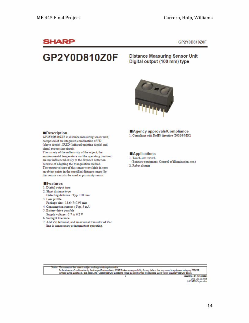
ME 445 Final Project Carrero, Holp, Williams
14

Remote Controlled, Capacitor Powered Coil Gun
P r e p a r e d f o r : D r . H e n r y J . S o m m e r I I I
M i c h a e l R o b i n s o n
T h e P e n n s y l v a n i a S t a t e U n i v e r s i t y
D e p a r t m e n t o f M e c h a n i c a l a n d N u c l e a r
E n g i n e e r i n g
M E 4 4 5
5 / 2 / 2 0 1 3
Taylor Hornung Jeffrey Chan

P a g e | 2
Abstract
This ME 445 Spring 2013 project sets out to make a coil gun on a two axis turret that is
controlled by a wireless PlayStation 2 controller. The main components for the project are: a coil
wrapped around a barrel, two servo motors, a PlayStation 2 controller, an Arduino Uno and ten
capacitors. The Arduino Uno is used to interface with the coil gun and turret, control the
movement of the turret, the firing of the projectile and the charging of the capacitors.
The coil gun works on the same principle as a solenoid which, with careful timing of the coil
current can launch iron or steel projectiles. The coil is wound over a non-magnetic barrel with
the projectile positioned at one end of the coil. When a short current pulse is passed through the
coil, the projectile will accelerate into the coil, and if this pulse is terminated just as the projectile
reaches the middle of the coil, will leave with an increase in velocity.
The coil gun for this project has two main circuits: a charging circuit and a firing circuit.
The charging circuit handles the charging of the ten 4700μF capacitors to 23V or 34V through
the use of a 100Ω, 2W power resistor, a TIP-29 transistor and an LED. The power resistor is
used to limit the amount of current flowing in the charging circuit to protect the capacitors from
a current surge. The TIP-29 is controlled by the Arduino and acts as a switch to turn on and off
the circuit. The LED is used to visually alert the user that the capacitors are being charged. The
capacitor’s stored charge supplies the current to the coil. For the firing circuit, the following
components are used: a power MOSFET, a coil, a flyback diode and a current sensing resistor.
The power MOSFET is a transistor used to turn on and off the firing circuit via the Arduino. The
coil induces a magnetic field, propelling the projectile forward. A flyback diode is used to
prevent reverse polarity across the electrolytic capacitors and to keep current looping through the
coil. A current sensing resistor allows for the measurement of the current through the coil for
evaluating the performance of the coil gun.
The coil gun is mounted on two servo motors that act as a stationary turret. These servos aim
the coil gun up and down (pitch) and side to side (yaw). The servos are controlled by the
Arduino, with the commands coming from a wireless PlayStation 2 controller. When the user
moves the analog joysticks up/down and left/right, the signals are received by the Arduino which
moves the servo motors to adjust the turret’s position accordingly.
Several iterations of coil designs were created and tested throughout the project. A large
quad coil was first made, having four separate coils connected in parallel to reduce the total
resistance and thereby increase the current when firing. The second coil constructed was a large
single coil tightly wrapped around a smaller barrel. The larger size increased inductance, but also
significantly increased resistance. The final coil made was a small tightly wrapped coil to keep
the induced magnetic field close to the projectile and to keep the resistance low.
Recording velocities and obtaining data to compare the different coils is done using an
optical switch, a current sensing resistor and a Personal Measurement Device, or PMD-1208.
The optical switch is mounted on the barrel at the end of the coil. When the projectile blocks the
light emitted by the switch, a speed is calculated by the Arduino. The speed data is then used to
compare the different coils and their efficiencies. After evaluating the coils, it could be seen that
although the coils have comparable velocities, the small coil is the most efficient as it produced
the highest velocity for the least amount of energy consumed. This design was mounted onto the
turret as the final coil gun design.

P a g e | 3
Table of Contents
Abstract ...................................................................................................................... 2
Table of Contents ....................................................................................................... 3
1 Introduction ......................................................................................................... 4
1.1 Project Description ........................................................................................................... 4
1.2 Objectives ......................................................................................................................... 4
2 Coil Design .......................................................................................................... 5
2.1 Multiple Parallel Coils ..................................................................................................... 5
2.2 Large Single Coil ............................................................................................................. 6
2.3 Small Single Coil ............................................................................................................. 7
3 PlayStation 2 Controller ...................................................................................... 8
3.1 Controller Hardware Configuration ................................................................................. 8
3.2 Controller Software Configuration................................................................................. 10
4 Charging and Triggering ...................................................................................12
4.1 Original Dual Switches .................................................................................................. 12
4.2 Arduino Controlled Switches ......................................................................................... 14
4.3 PlayStation Controlled Switches .................................................................................... 16
4.4 Safety Discharge Switch ................................................................................................ 17
5 Turret Mounting ................................................................................................18
5.1 Turret Construction and Hardware ................................................................................. 18
5.2 Turret Control ................................................................................................................. 19
5.3 Turret Upgrades and Improvements ............................................................................... 20
6 Timing and Speed..............................................................................................21
6.1 Timing For Current Duration ......................................................................................... 21
6.2 Timing for Speed Measurements ................................................................................... 23
7 Testing and Results ...........................................................................................26
7.1 Testing Methodology and Setup .................................................................................... 26
7.2 Final Results ................................................................................................................... 27
8 Conclusion .........................................................................................................32
Appendix ..................................................................................................................33
A.1 Hardware Schematic ...................................................................................................... 33
A.2 Bill of Materials ............................................................................................................. 34
A.3 Data Sheets for Relevant Components ........................................................................... 35
A.4 Arduino Code ................................................................................................................. 39
A.5 Simulink Models of Coil Gun ........................................................................................ 43
A.6 Matlab Simulation Code................................................................................................. 44
A.7 Matlab Data Gathering Code.......................................................................................... 45

P a g e | 4
1 Introduction
1.1 Project Description
A coil gun is a device composed of one or more coils in an electromagnet configuration
used to accelerate a ferromagnetic projectile. A coil gun works on the basis of a solenoid which
can launch iron or steel projectiles through the careful timing of the coil current. The coil is
wound over a non-magnetic barrel while the projectile is positioned at one end of the coil. If a
short current pulse is passed through the coil, the projectile will accelerate into the coil, and if
this pulse is terminated just as the projectile reaches the middle of the coil, the projectile will
continue to move forward, leaving the barrel. One of the most important aspects of coil gun
design is the correct timing and shaping of the current pulse.
Figure 1: Coil Gun Example
(Image Source: http://www.coilgun.eclipse.co.uk/coilgun_basics_1.html)
When current flows in a coil, it generates a magnetic field with a direction given by the
right hand rule. The ferromagnetic projectile is then attracted to the center of the coil by the
induced magnetic field of the coil.
1.2 Objectives
This project will explore the following concepts: electromagnetism, using the Arduino as
a controller, interfacing the Arduino to the coil gun, and learning about individual electronic
components and their uses. The following is a list of goals to achieve for this project. There are
five main objectives which deal with creating an effective coil gun, as well as a smooth interface
to operate the gun both in firing and aiming.
Create a single stage coil gun powered by capacitors
Mount the coil gun on a stationary, two-axis turret
Control the charging, firing, and turret motion using a wireless PlayStation 2
controller
Develop a timing system for the current pulse to provide maximum projectile
velocity
Be able to gather data on projectile muzzle velocity directly from the program

P a g e | 5
2 Coil Design
The coil that is mounted on the turret is the product of many design iterations and prototype
tests. Many coils were fabricated but three main coils stood out during the development process.
These coils were: a quad coil hooked up in parallel, a large coil fabricated from an entire spool of
24 gauge wire and a tightly wrapped small coil. The results of the different coils are discussed in
Section 7 Testing and Results.
2.1 Multiple Parallel Coils
The first coil built was the quad coil, depicted in Figure 2. This coil consisted of four
individual coils that were wrapped around the barrel. The barrel is a mechanical pencil that was
stripped down to its outer shell and subsequently wrapped with 20 gauge enameled copper wire.
The coil was created by wrapping the wire by hand between the stoppers. Two coils were
wrapped next to each other and held together by the stoppers and compressed together by rubber
bands. Two additional coils were wrapped over the first two coils, making this coil a quad coil
design. To keep the total resistance of the coil to a minimum, each individual coil was then
connected in parallel to the electrical circuit. The concept behind this coil was to increase the
inductance while keeping the resistance as low as possible. Since the effective coil resistance is
low, large amounts of current can pass through the coil and in turn induce large magnetic fields
within the four coils. The result of this coil was as predicted, resistance was low, 0.3Ω, and
inductance was high, with its many wraps. However, although the coil had low resistance and
high current levels, the nail did not shoot out of the barrel as fast as expected. This is because a
magnetic field generated by current reduces in strength by the square of the coil’s radius.
Therefore the farther away from the center the wraps are, the less the magnetic field contributes
to moving the projectile. This means that the two outer coils provided only minimal benefit to
the overall performance of the coil. Even though the coil had a low resistance, the extra wire
used for the outer two wraps did not provide a favorable tradeoff between a gain in inductance
and lower resistance by having more coils in parallel. Thus the efficiency of the quad coil was
very low (See Section 7) and a new coil with a single coil that was tightly wrapped was made.
Figure 2: Quad Coil Connected in Parallel

P a g e | 6
2.2 Large Single Coil
The next coil was designed to attempt to maximize the inductance of the coil by making it
as large as possible. This design features a coil that is tightly wrapped with the largest number of
turns to maximize inductance, shown in Figure 3. Differences between the quad coil and the
single large coil are: the barrel is now made of stainless steel, 24 gauge enameled copper wire is
used for the winding, and the barrel is smaller in diameter. The coil was wrapped using a power
drill, making the fabrication of the coil faster and allowing for tighter wraps. For this coil, the
smaller wire was chosen to increase the number of wraps possible in the limited space. However,
the smaller wire resulted in a significant increase in resistance. The result of this coil was large
inductance but high resistance (6Ω). This coil was unable to fire the projectile due to the
resultant current being so low. With the same 23V capacitor voltage as the quad coil, the current
across the large coil peaked at less than 5 amps; not enough to create a magnetic field strong
enough to move the projectile. In an attempt to reduce the resistance, half of the wraps were
removed resulting in a reduced coil (Figure 4) with a resistance of 3Ω. Although this reduced
coil provided a low enough resistance to generate a current high enough to induce a magnetic
field, it still could not fire the projectile with any consistency. The coil was ultimately a failure
because the barrel used was stainless steel. Instead of increasing the strength of the magnetic
field, the barrel became magnetized and prevented the projectile from firing.
Figure 3: Large Single Coil
Figure 4: Reduced Single Coil

P a g e | 7
2.3 Small Single Coil
From everything learned from previous coils, a small single coil was chosen for the final
design, shown in Figure 5. This coil was designed to be as tightly wrapped as possible but small
enough so that the resistance would not hinder the current flow. Only five passes were used to
keep each wrap as close to the center as possible. This tightly wrapped design allows the outer
most wraps to significantly contribute to the induced magnetic field. The barrel also has a
significantly smaller diameter allowing the coils to be as close to the projectile as possible. In
addition, the barrel was first wrapped in a layer of Mu-metal, a nickel-iron alloy designed to
focus the magnetic field without the problems associated with a metal barrel. Subsequently, a
piece of stainless steel was wrapped around the outside of the coil to provide extra shielding. The
coil was wrapped using a power drill to ensure a tightly wrapped coil. 28 gauge wire was used to
increase inductance, resulting in a coil with approximately 350 wraps over a length of 1 inch.
This provided an efficient coil with approximately 1.9 Ω of resistance. Although the inductance
and current are lower than the quad coil design, the efficiency of the small coil is much higher
since all of the current is used to generate a strong magnetic field instead of being wasted in coils
that are too far away from the projectile.
Figure 5: Small Single Coil with Shielding

P a g e | 8
3 PlayStation 2 Controller
3.1 Controller Hardware Configuration
To control the coil gun and turret, a wireless PlayStation 2 controller, shown in Figure 6,
was used. To interface with this controller, the nine pin wireless receiver, shown in Figure 7,
must be connected directly to the Arduino. The pins on the wireless receiver that are used are
Data, Command, Attention, Clock, and 3.3V and GND to power the receiver. Figure 8 shows the
wireless receiver after being disassembled and with the new jumper wires directly soldered to the
required output lines. Figure 9 illustrates which pins from the controller receiver are connected to
which lines for soldering.
Figure 6: Wireless PlayStation 2 Controller
Figure 7: Wireless PlayStation 2 Receiver
Figure 8: Wireless PlayStation 2 Receiver Circuit Board
Wiring
Figure 9: Wiring Breakdown for PlayStation 2 Receiver
(Image Source: CuriousInventor.com)

P a g e | 9
The wiring schematic for connection of the PlayStation 2 wireless receiver to the Arduino
is shown in Figure 10. The four signal lines are connected directly to the Arduino’s digital input
pins which allows the Arduino to communicate directly with the controller.
Figure 10: Wiring Schematic for PlayStation 2 Wireless Receiver to Arduino

P a g e | 10
3.2 Controller Software Configuration
To communicate with the PlayStation controller, several lines of code were added to the
program. The first block of code includes the PS2 library of commands into the program and
creates a controller object.
#include <PS2X_lib.h> // include the ps2 controller library
// PS2 Controller
PS2X ps2x; // create PS2 Controller Class
int error = 0; // errors in connecting the PS2 controller
byte type = 0; // type of PS2 controller
byte vibrate = 0;
The next block of code is located in the program setup routine. The “error =” line configures
the PS2 controller object and returns a number if any errors are encountered. The following lines
display the corresponding error message if one exists.
// setup pins and settings: GamePad(clock, command, attention, data,
Pressures?, Rumble?) check for error
// wire color left to right white, orange, blue, purple
error = ps2x.config_gamepad(2,5,3,4, false, false);
if(error == 0)
Serial.println("Found Controller, configured successful.");
else if(error == 1)
Serial.println("No controller found,\nCheck wiring, see readme.txt to
enable debug.\nVisit www.billporter.info for troubleshooting tips.");
else if(error == 2)
Serial.println("Controller found but not accepting commands.\nSee
readme.txt to enable debug.\nVisit www.billporter.info for troubleshooting
tips.");
else if(error == 3)
Serial.println("Controller refusing to enter Pressures mode, may
not support it. ");

P a g e | 11
The final block of code in the setup routine determines the type of PlayStation controller that
has been connected and displays a message accordingly.
type = ps2x.readType(); // Check what type of controller is attached
switch(type)
case 0:
Serial.println("Unknown Controller type");
break;
case 1:
Serial.println("DualShock Controller Found");
break;
case 2:
Serial.println("GuitarHero Controller Found");
break;
Finally, in the main program loop the Arduino reads the state of the controller, or
gamepad, and loads the state of each button and joystick into the controller object. It is important
to include a small delay in the program loop so that the Arduino has time to read the state of the
controller. If the delay is too small (<16ms), or there is no delay, the program will not be able to
finish reading the controller before it attempts to read it again, resulting in a non-responsive
game controller. The wireless controllers are especially prone to this problem. Likewise it is
important to read the controller at least once every 2 seconds. Less often and the controller will
leave analog mode.
// Read the state of the pushbuttons and yaw/pitch joysticks:
// Read the PS2 Controller
ps2x.read_gamepad();
.
.
.
delay(30);

P a g e | 12
4 Charging and Triggering
4.1 Original Dual Switches
The original coil gun was built and operated manually for proof of concept. With no
Arduino, the charging and firing of the gun was performed with two physical switches. The first
switch, SW1 in Figure 11, was used for charging. When this switch was closed, the capacitor
bank was connected to the power supply through the charging resistor (R1). Once the capacitors
reached their maximum voltage, this switch was opened, disconnecting the charging loop. To fire
the gun, a large SPST switch, SW2 in Figure 11, was used. When this switch was closed, the
capacitor bank discharged directly through the coil. A flyback diode, (D2), was used to prevent
reversing of the voltage polarity on the capacitors and to prevent oscillating voltage spikes on the
coil. This system was only used for proof of concept and was replaced by an Arduino controller
firing mechanism.
Figure 11: Manually Triggered Coil Gun Schematic

P a g e | 13
The charging loop is highlighted in green in Figure 12. The firing loop is highlighted in
red in Figure 13. Only one switch can be closed at a time to ensure the system does not short.
Figure 12: Charging Loop for Manually Triggered Coil Gun
Figure 13: Firing Loop for Manually Triggered Coil Gun

P a g e | 14
4.2 Arduino Controlled Switches
To replace the manual switches, an Arduino was used with two transistors to activate the
charging and firing circuits. The two switches were moved out of the coil circuit and onto a small
Arduino circuit. In this configuration the switches, SW1 and SW2 shown in Figure 14, could be
used to set an Arduino digital input pin HIGH. This signal would active a section of code that
would turn on the respective transistor. Using this method also allows for a software safety check
to ensure that both the charging and firing circuits will not be energized at the same time causing
a short circuit.
To avoid high voltage and current spikes from damaging the Arduino, a PS2501-2 optical
isolator was used to ensure the complete separation of the coil gun circuit from the Arduino’s
circuit. This added a second layer of protection in addition to the transistors.
Figure 14: Arduino Triggered Coil Gun Schematic

P a g e | 15
An example of how the switching system works is shown in Figure 15. The example is
done for the charging scenario. When SW1 is closed, Arduino pin 3 goes high. The software then
sets the Arduino pin 9 high. This activates the optical isolator which sets the base of the TIP 29
high. Lines that are HIGH are shown in yellow. The charging loop is highlighted in green.
Figure 15: Arduino Controlled Switching System for Charging Loop
5V
Line
Ard
uin
o U
no

P a g e | 16
4.3 PlayStation Controlled Switches
To completely replace the original physical switches in the circuit, a PlayStation 2
controller was configured to activate the Arduino code that charges and fires the coil gun. The
only change from the previous configuration is that instead of a physical switch setting an
Arduino input pin high, a button is used on the PS2 controller to activate the software.
The first block of code (***CHARGING***) is broken into two sections. The first
determines whether the charging button on the PS2 controller (red) is pressed and whether the
gun is charging or not and sets the charging state of the gun accordingly. The second section sets
the Arduino output pin (chargingPin = 9) to HIGH or LOW depending on the charging state of
the gun.
// *** CHARGING ***
if(ps2x.ButtonPressed(PSB_RED) && chargingState == 0)
chargingState = 1;
Serial.println("Gun is charging.");
else if(ps2x.ButtonPressed(PSB_RED) && chargingState == 1)
chargingState = 0;
Serial.println("Charging complete.");
if (chargingState == 1) // only charge if the charge button is
pressed
digitalWrite(chargingPin,HIGH);
else
digitalWrite(chargingPin,LOW);
The second block of code (***TRIGGERING***) sends the software into the
“firing=true” loop when the firing button is pressed (blue). This is where the software safety
check is implemented. If the gun is charging, i.e., the charging loop is closed, the software will
prevent the user from closing the firing loop and causing a short circuit.
// *** TRIGGERING ***
if(ps2x.ButtonPressed(PSB_BLUE) && chargingState == 0 && firing ==
false) // only fire gun if it's not charging
firing = true;
Serial.println("Firing!\n");
else if(ps2x.ButtonPressed(PSB_BLUE) && chargingState == 1)
firing = false;
Serial.println("Stop charging before attempting to fire.");

P a g e | 17
4.4 Safety Discharge Switch
To avoid the hazard of leaving a large set of capacitors charged to a high voltage, a safety
switch was implemented, shown as SW3 in Figure 16, (SW in final schematic). When the switch
is closed, the capacitors are connected to a resistor in a simple RC circuit to provide a safe way
to discharge the system. For safety considerations, the switch was kept as a physical push button
instead of a software based switch. This allowed the circuit to be discharged manually if
necessary, regardless of whether the Arduino was plugged in or not.
Figure 16: Safety Discharge Switch Schematic
Figure 17 shows the loop for discharging, highlighted in blue.
Figure 17: Safety Discharge Switch Loop

P a g e | 18
5 Turret Mounting
5.1 Turret Construction and Hardware
One of the goals of the project was to mount the coil gun on a two-axis turret for aiming.
Several ideas were generated for the construction of the turret. Original designs included wooden
components and a 3D printed stand to mount the servos on. This original design would allow for
a custom mounting arrangement for the servos. Ultimately, the final design used acrylic plates
for the turret. Acrylic is easy to machine to size and to drill holes in. Metal brackets were used in
conjunction with machine screws to attach the plates together. This design provides a stable
platform for the gun that can be easily disassembled and modified if necessary.
Figure 18: Turret Mounting Plates and Brackets
Two RC servos are used to control the motion of the turret in the yaw (side to side) and
pitch (up/down) directions. Each servo is powered directly by the Arduino’s 5V line. The signal
lines for the servos are connected to the Arduino’s digital pins as outputs, shown in Figure 19.
Figure 19: Turret Servo Wiring Schematic
Acrylic Plates
Brackets and Bolts
Turret Servos

P a g e | 19
5.2 Turret Control
The PlayStation 2 controller has two analog joysticks which were used to control the two
servos for the turret. The right joystick was used to control the pitch of the turret by either
pushing the joystick forward or pulling it back. The left joystick was used to control the yaw
motion of the turret by moving the joystick side to side.
The first block of code adds or subtracts the joystick’s position from a counter and
constrains this counter between ±turretspeed. If the turretspeed variable is set lower, the counter
will reach its maximum value quicker. This counter acts as a pseudo version of the servo’s actual
position, and hence adjusting the limits is a quick way to adjust the speed of the servos.
However, there was one problem encountered if this section of code was run every program
loop. The analog value returned from the controller would occasionally read a maximum value
when it should have read zero, i.e., the joystick is not touched but still sends occasional blips of
data. To avoid these blips of data from adding to the servo position counter, an IF statement was
added to ensure that the turret position is only updated if either the L1or R1 buttons are held
down.
// *** TURRET CONTROL ***
if(ps2x.Button(PSB_L1) || ps2x.Button(PSB_R1)) // print stick values if either is TRUE
yawPosition = constrain(yawPosition + ps2x.Analog(PSS_LX)-128,-turretspeed,turretspeed);
pitchPosition = constrain(pitchPosition + ps2x.Analog(PSS_RY)-128,-
turretspeed,turretspeed);
// The above 2 lines set a pseudo position that is adjusted based on the controller joysticks
and constrained
// to the turret speed. A shorter turret speed will reach the servo limits quicker
The second block of code writes the desired position to each servo. The position of the
servo is restricted to a user defined limit, set in the beginning of the program code. yawLimits[]
and pitchLimits[] are two value arrays that set the min and max position that the servo should be
allowed to move to avoid damaging the wires or colliding the barrel into the turret base.
Servo.writeMicroseconds() is used instead of Servo.write() to provide a smoother servo motion,
as discussed in Section 5.3 Turret Upgrades and Improvements.
yawServo.writeMicroseconds(map(yawPosition,-
turretspeed,turretspeed,yawLimits[0]+105,yawLimits[1]+105)*50/9+1000);
pitchServo.writeMicroseconds(map(pitchPosition,-
turretspeed,turretspeed,pitchLimits[0]+90,pitchLimits[1]+90)*50/9+1000);
// The above 2 lines write the servo position to the servo in us. 1000-2000, 1500 at center.
// The pseudo position is mapped to the actual position here.
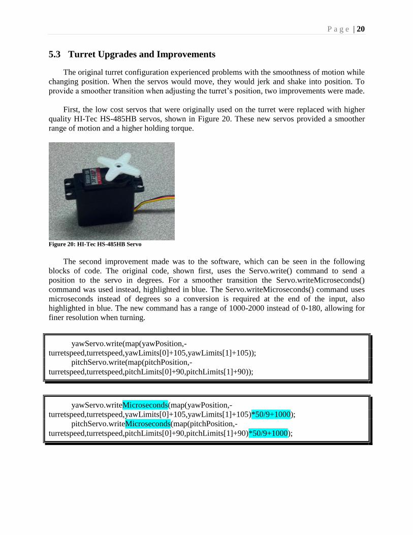
P a g e | 20
5.3 Turret Upgrades and Improvements
The original turret configuration experienced problems with the smoothness of motion while
changing position. When the servos would move, they would jerk and shake into position. To
provide a smoother transition when adjusting the turret’s position, two improvements were made.
First, the low cost servos that were originally used on the turret were replaced with higher
quality HI-Tec HS-485HB servos, shown in Figure 20. These new servos provided a smoother
range of motion and a higher holding torque.
Figure 20: HI-Tec HS-485HB Servo
The second improvement made was to the software, which can be seen in the following
blocks of code. The original code, shown first, uses the Servo.write() command to send a
position to the servo in degrees. For a smoother transition the Servo.writeMicroseconds()
command was used instead, highlighted in blue. The Servo.writeMicroseconds() command uses
microseconds instead of degrees so a conversion is required at the end of the input, also
highlighted in blue. The new command has a range of 1000-2000 instead of 0-180, allowing for
finer resolution when turning.
yawServo.write(map(yawPosition,-
turretspeed,turretspeed,yawLimits[0]+105,yawLimits[1]+105));
pitchServo.write(map(pitchPosition,-
turretspeed,turretspeed,pitchLimits[0]+90,pitchLimits[1]+90));
yawServo.writeMicroseconds(map(yawPosition,-
turretspeed,turretspeed,yawLimits[0]+105,yawLimits[1]+105)*50/9+1000);
pitchServo.writeMicroseconds(map(pitchPosition,-
turretspeed,turretspeed,pitchLimits[0]+90,pitchLimits[1]+90)*50/9+1000);

P a g e | 21
6 Timing and Speed
6.1 Timing For Current Duration
Timing is an important aspect of configuring a coil gun to ensure that it achieves optimal
performance. Timing refers to the act of shutting off the current supplied to the coil at a specified
time. The heart of a coil gun is a solenoid generating a magnetic field. When current is passed
through the coil a magnetic field is generated which attracts the projectile. However, if the
current continues to flow throughout the duration of the firing sequence, the projectile will lurch
forward and then experience “suck-back” and be pulled into the center of the coil to align with
the magnetic field. To ensure that the projectile leaves the barrel with maximum speed, this
“suck-back” effect must be eliminated by shutting off the current at precisely the correct time. If
the current remains on too long, the projectile will experience “suck-back” and be propelled at a
slower speed. If the current is shut off too soon, the coil will not impart the maximum amount of
energy to the projectile.
The original plan to eliminate “suck-back” involved using an optical switch to detect when
the projectile was about to leave the barrel. This method was implemented on several coils, but
did not provide optimal results. The switch used was an infrared LED and phototransistor, shown
in Figure 21. The switch was installed in the sides of the barrel of the gun at the end of the coil
(Figure 22). However, it was determined that by the time the projectile reached the optical
switch, it was already too late to turn off the current. This sensor was still used to determine the
speed of the projectile discussed in section 6.2 Timing for Speed Measurements.
Figure 21: Infrared Emitter and Phototransistor For Timing
Figure 22: Optical Switch Hot-Glued Into Barrel at End of Coil

P a g e | 22
Since a dynamic switching system could not be implemented easily, a hardcoded method
was used to time the current shut-off. At a specified time after the firing sequence begins, the
current is forced off by shutting of the transistor. Trial and error was used to determine the
optimal shut-off time. Figure 23 shows a plot comparing projectile speed to shut-off time. The
following block of code demonstrates how the Arduino would shut off the current after an
elapsed time of 5300µs, which was found to be the approximate optimal time for the 33V
configuration, as seen in Figure 23. This configuration was also found to be the most efficient of
the settings tested.
if ((micros()-launchTime) < 5300) // 6350 for 24V 5300 for 33V
digitalWrite(triggerPin,HIGH); // write HIGH until specified time has elapsed
// this will allow current to flow through the coil
else
digitalWrite(triggerPin,LOW);
Figure 23: Graph to Determine Optimal Shut-Off Time For Current at 47mF, 33V
1.45%
1.50%
1.55%
1.60%
1.65%
1.70%
1.75%
17.6
17.8
18
18.2
18.4
18.6
18.8
19
19.2
19.4
19.6
19.8
20
4500 4700 4900 5100 5300 5500 5700 5900 6100 6300 6500
Effi
cie
ncy
(%
)
Pro
ject
ile S
pe
ed
(m
ph
)
Current Duration (µs)
Projectile Speed and Coil Gun Efficiency vs. Current Duration
Speed
Efficiency

P a g e | 23
6.2 Timing for Speed Measurements
To determine the performance of the coil gun, the speed of the projectile was measured as it
left the barrel. The optical switch shown in Figure 21 and Figure 22 was used for this purpose.
Since the current will have already been turned off by the time the projectile reaches this switch,
the projectile will not be accelerating, and its muzzle velocity can be accurately measured. To
measure the projectile’s speed, the following process was used. When the projectile first breaks
the optical switch beam, the run-time of the program is recorded. When the back of the projectile
passes the beam and turns the switch back on, the run time of the program is recorded once
again. The length of the projectile is then divided by the difference between these two run times
and converted to miles per hour to calculate the final speed. The following block of Arduino
code demonstrates how this is accomplished.
switchState = digitalRead(opticalSwitch); // check the optical switch
if (switchState == 0 && timing == 2) // if the projectile is completely past the switch
endTime = micros(); // time at which the projectile leaves the coil completely
time1 = leaveTime-launchTime; // time until projectile got to switch
time2 = endTime-leaveTime; // time the projectile blocked the switch
Speed = length/12*3600000/5280/float(time2)*1000; // Convert to mph
timing = 0; // reset timing
firing = false; // reset firing state
// Display the projectile speed and launch time
Serial.println("LAUNCH TIME(us) SPEED (mph)");
Serial.print(time1);
Serial.print("\t\t\t");
Serial.println(Speed);
Serial.println("=========================================\n");
delay(1000); // wait one second to return control to the user
// this ensures the projectile is gone before attempting to fire again
else if (switchState == 1 && timing == 1) // if projectile is moving and has reached end
of coil
leaveTime = micros(); // projectile is starting to leave coil
timing = 2; // projectile is blocking the optical switch
digitalWrite(triggerPin,LOW); // turn off the current
// end else if

P a g e | 24
The initial coil design presented problems with the optical switch because of the size of the
barrel. Since the projectile had a significantly smaller diameter than the barrel (nail compared to
pencil tube), it would actually travel beneath the sensor beam, and never trigger the switch, as
illustrated in Figure 24. To resolve this issue, the sensor was placed vertically so that the beam
would be more directly in the path of the projectile (Figure 25).
However, because the projectile was still significantly smaller than the barrel, it would tend
to move side-to-side during launch (Figure 26). This would cause the projectile to break the
sensor beam for inaccurate amounts of time, resulting in occasional erroneous velocity data. To
resolve this issue, a much smaller barrel was used for the final design (Figure 27) which allowed
for no extraneous movements of the projectile, in addition to permitting a tighter wrapped coil.
Figure 24: Original Barrel with Horizontal Optical Sensor, Front View
Figure 25: Original Barrel with Vertical Optical Sensor, Front View
Projectile
Sensor Beam
Projectile
Sensor Beam

P a g e | 25
Figure 26: Original Barrel with Vertical Sensor, Top View
Figure 27: Final Barrel with Horizontal Sensor, Front View
Projectile Sensor Beam
Projectile
Sensor Beam
Inaccurate Sensor Timing
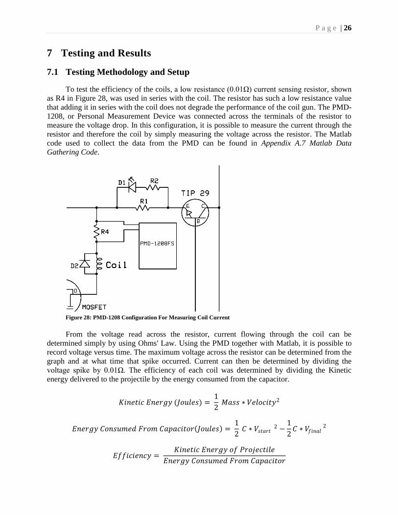
P a g e | 26
7 Testing and Results
7.1 Testing Methodology and Setup
To test the efficiency of the coils, a low resistance (0.01Ω) current sensing resistor, shown
as R4 in Figure 28, was used in series with the coil. The resistor has such a low resistance value
that adding it in series with the coil does not degrade the performance of the coil gun. The PMD-
1208, or Personal Measurement Device was connected across the terminals of the resistor to
measure the voltage drop. In this configuration, it is possible to measure the current through the
resistor and therefore the coil by simply measuring the voltage across the resistor. The Matlab
code used to collect the data from the PMD can be found in Appendix A.7 Matlab Data
Gathering Code.
Figure 28: PMD-1208 Configuration For Measuring Coil Current
From the voltage read across the resistor, current flowing through the coil can be
determined simply by using Ohms' Law. Using the PMD together with Matlab, it is possible to
record voltage versus time. The maximum voltage across the resistor can be determined from the
graph and at what time that spike occurred. Current can then be determined by dividing the
voltage spike by 0.01Ω. The efficiency of each coil was determined by dividing the Kinetic
energy delivered to the projectile by the energy consumed from the capacitor.
𝐾𝑖𝑛𝑒𝑡𝑖𝑐 𝐸𝑛𝑒𝑟𝑔𝑦 (𝐽𝑜𝑢𝑙𝑒𝑠) = 1
2 𝑀𝑎𝑠𝑠 ∗ 𝑉𝑒𝑙𝑜𝑐𝑖𝑡𝑦2
𝐸𝑛𝑒𝑟𝑔𝑦 𝐶𝑜𝑛𝑠𝑢𝑚𝑒𝑑 𝐹𝑟𝑜𝑚 𝐶𝑎𝑝𝑎𝑐𝑖𝑡𝑜𝑟 𝐽𝑜𝑢𝑙𝑒𝑠 = 1
2 𝐶 ∗ 𝑉𝑠𝑡𝑎𝑟𝑡 2 −
1
2𝐶 ∗ 𝑉𝑓𝑖𝑛𝑎𝑙
2
𝐸𝑓𝑓𝑖𝑐𝑖𝑒𝑛𝑐𝑦 = 𝐾𝑖𝑛𝑒𝑡𝑖𝑐 𝐸𝑛𝑒𝑟𝑔𝑦 𝑜𝑓 𝑃𝑟𝑜𝑗𝑒𝑐𝑡𝑖𝑙𝑒
𝐸𝑛𝑒𝑟𝑔𝑦 𝐶𝑜𝑛𝑠𝑢𝑚𝑒𝑑 𝐹𝑟𝑜𝑚 𝐶𝑎𝑝𝑎𝑐𝑖𝑡𝑜𝑟

P a g e | 27
7.2 Final Results
All of the coils were tested under various conditions using the current resistor and the PMD
as described in Section 7.1, and their results are displayed below.
Quad Coil:
Figure 29: Quad Coil Experimental Results (23V, 0.047F)
LAUNCH TIME (µs) SPEED (mph) EFFICIENCY (%)
9460 15.91 0.441
The Quad coil results demonstrate the concept of having multiple coils in parallel to
lower resistance; voltage peaked at 1.832V and thus current at 183.2A. 183A is the largest
amount of current achieved compared to all the other coils. The speed of the projectile was not as
fast as expected, launching out at 15.91 mph thereby confirming the theory that magnetic field
strength reduces by radius² of the coil windings, and significantly lowers the effectiveness of the
coil. Therefore the tradeoff of reduction in resistance to the gain of inductance was low,
decreasing the efficiency of the coil to less than 0.5%. In addition, the voltage remaining on the
capacitors was 14.5V; indicating that the quad coil used 7.49J of energy, nearly four times more
than the small coil. The gain in inductance from the two outer coils did not have a strong impact
on the speed of the projectile since they were too far from the projectile. From the quad coil, it
was concluded that parallel coils lower the resistance but are less efficient since most of the
added current is wasted.
0.55 0.6 0.65 0.7 0.75 0.8 0.85 0.9 0.95 1 1.05
0
0.2
0.4
0.6
0.8
1
1.2
1.4
1.6
1.8X: 0.8115
Y: 1.832
Time [sec]
Channel 0 [
V]

P a g e | 28
Small Single Coil:
Figure 30: Small Single Coil Experimental Results (23V, 0.047F)
LAUNCH TIME (µs) SPEED (mph) EFFICIENCY (%)
8284 15.49 1.676
From the results above, it can be seen that the small single coil has a peak voltage of
0.2491V and a peak current of 24.91A. Although the peak current through the small coil is
significantly less than the quad coil, the projectile speeds are comparable. After firing, there was
21.2V remaining on the capacitors; indicating that the small coil only used around 1.87J of
energy, far less than the quad coil at 7.49J. This proves that a tightly wrapped coil is more
efficient than a large coil as the small coil used less energy for a comparable projectile speed.
These results proved the hypothesis that a small, tightly wrapped coil with low resistance is the
most efficient coil design.
0.75 0.8 0.85 0.9 0.95 1
0.05
0.1
0.15
0.2
X: 0.8007
Y: 0.2491
Time [sec]
Channel 0 [
V]

P a g e | 29
Half Capacitance:
Figure 31: Small Single Coil at Half Capacitance Experimental Results (23V, 0.0235F)
LAUNCH TIME (µs) SPEED (mph) EFFICIENCY (%)
8024 14.69 1.804
From the half-capacitance test it can be seen that lower capacitance may provide slightly
higher efficiency for a short range of values. However, this comes at a cost. With significantly
lower capacitance, the energy storage capability is much less and the result is a lower current
(17.09A) and slower speed. The voltage remaining on the capacitors after this test was 19.9V, so
although a larger voltage drop occurred, the starting energy was reduced resulting in higher
efficiency. If the capacitance were reduced too far, without increasing the voltage to compensate
for the reduction in available energy, there would eventually be too little energy available to
move the projectile and therefore efficiency would decline towards zero. For the scope of this
project, this optimal point was not determined, especially since the result would likely be a
slower projectile speed.
0.43 0.44 0.45 0.46 0.47 0.48 0.49
0.02
0.04
0.06
0.08
0.1
0.12
0.14
0.16X: 0.4466
Y: 0.1709
Time [sec]
Channel 0 [
V]

P a g e | 30
Higher Voltage:
Figure 32: Small Single Coil at High Voltage Experimental Results (33V, 0.047F)
LAUNCH TIME (µs) SPEED (mph) EFFICIENCY (%)
6248 19.405 1.811
Additional tests at higher voltages provided the best results. Increasing the voltage to 33V
improved efficiency to 1.811% and significantly improved speed to almost 20mph. As was
expected, the higher voltage also resulted in a higher peak current of 35.65A, resulting in a
stronger magnetic field. Although the system used more energy, 2.716J compared to 1.870J, it
was able to impart far more kinetic energy to the projectile giving it a higher velocity. Ideally the
voltage would be increased as far as possible; however this is limited by the voltage rating of the
capacitors which was 35V for this project.
0.36 0.37 0.38 0.39 0.4 0.410
0.05
0.1
0.15
0.2
0.25
0.3
0.35X: 0.3794
Y: 0.3565
Time [sec]
Channel 0 [
V]
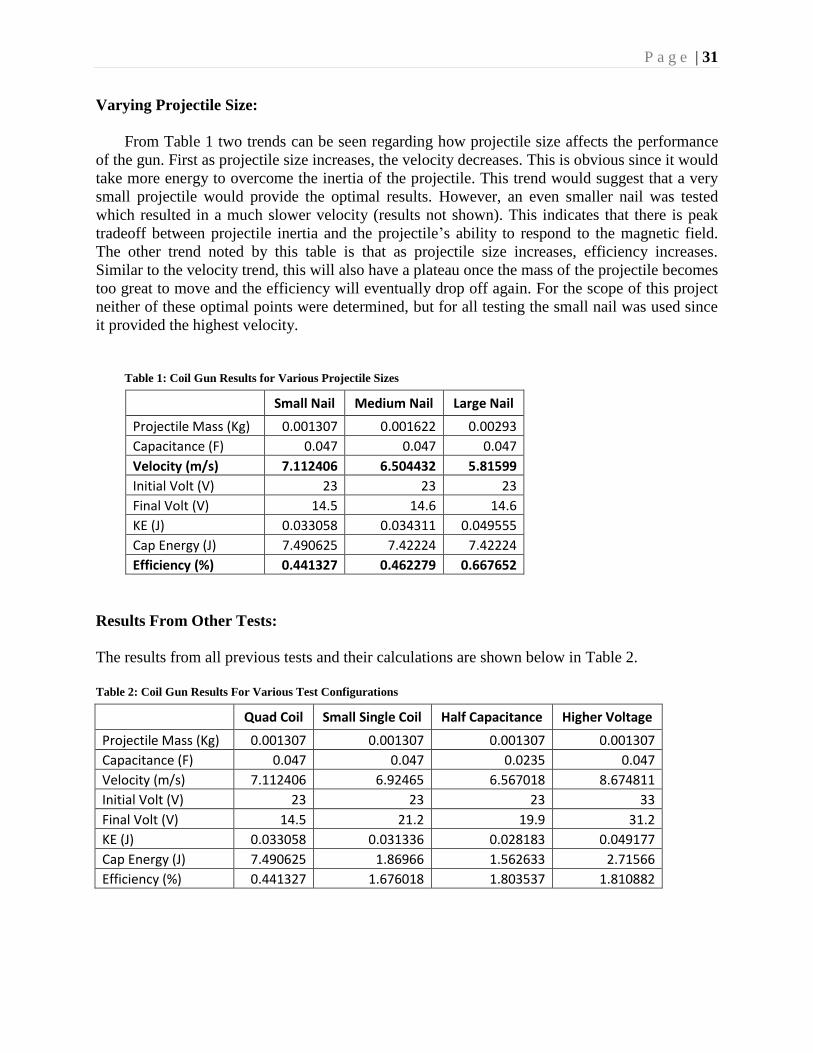
P a g e | 31
Varying Projectile Size:
From Table 1 two trends can be seen regarding how projectile size affects the performance
of the gun. First as projectile size increases, the velocity decreases. This is obvious since it would
take more energy to overcome the inertia of the projectile. This trend would suggest that a very
small projectile would provide the optimal results. However, an even smaller nail was tested
which resulted in a much slower velocity (results not shown). This indicates that there is peak
tradeoff between projectile inertia and the projectile’s ability to respond to the magnetic field.
The other trend noted by this table is that as projectile size increases, efficiency increases.
Similar to the velocity trend, this will also have a plateau once the mass of the projectile becomes
too great to move and the efficiency will eventually drop off again. For the scope of this project
neither of these optimal points were determined, but for all testing the small nail was used since
it provided the highest velocity.
Table 1: Coil Gun Results for Various Projectile Sizes
Small Nail Medium Nail Large Nail
Projectile Mass (Kg) 0.001307 0.001622 0.00293 Capacitance (F) 0.047 0.047 0.047 Velocity (m/s) 7.112406 6.504432 5.81599 Initial Volt (V) 23 23 23 Final Volt (V) 14.5 14.6 14.6 KE (J) 0.033058 0.034311 0.049555 Cap Energy (J) 7.490625 7.42224 7.42224 Efficiency (%) 0.441327 0.462279 0.667652
Results From Other Tests:
The results from all previous tests and their calculations are shown below in Table 2.
Table 2: Coil Gun Results For Various Test Configurations
Quad Coil Small Single Coil Half Capacitance Higher Voltage
Projectile Mass (Kg) 0.001307 0.001307 0.001307 0.001307 Capacitance (F) 0.047 0.047 0.0235 0.047 Velocity (m/s) 7.112406 6.92465 6.567018 8.674811 Initial Volt (V) 23 23 23 33
Final Volt (V) 14.5 21.2 19.9 31.2 KE (J) 0.033058 0.031336 0.028183 0.049177 Cap Energy (J) 7.490625 1.86966 1.562633 2.71566 Efficiency (%) 0.441327 1.676018 1.803537 1.810882

P a g e | 32
8 Conclusion
Overall, the project was a huge success since every objective set for the project was met. In
addition, the concepts covered during lecture were implemented and put to practice with the
development of this project. The final coil gun design implemented is the culmination of various
design iterations and research on coils, resulting in the most efficient of all the coils made for the
project. The capacitors are used to power the coil gun and are successful in their implementation.
This satisfies the objective of making a single stage coil gun powered by capacitors. The two
servo motors were connected to the coil, making the coil gun into a stationary cannon with
elevation (pitch) and side to side (yaw) movement. The Arduino controls the charging, firing and
motion of the coil gun via the use of a wireless PlayStation 2 controller. Timing the coil using
the Arduino to shut off the current, allowing the projectile to be launched at maximum speed,
was accomplished and proven successful via testing. The optical switch and the current sensing
resistor allowed for data collection and comparison between the coils and to calculate the
efficiencies of the coils.
The final coil design has an efficiency of 1.68%, which is comparable to other designs that
were researched prior to the start of the project. This efficiency level is within the same order of
magnitude as other designs thus proving the validity of the coil efficiency calculations.
Improvements can be made for the design of a coil gun, as proven by the test results, and
provided more time, the following improvements could be made:
Make a multi-stage coil, synchronizing the firing of each coil
Implement a dynamic timing system allowing for the current to shut off at a time
determined by the position of the projectile in the barrel using the optical switch
Use higher rated capacitors for more energy
Charge the capacitors to a higher voltage via the use of transformers to drastically
increase voltage

P a g e | 33
Appendix
A.1 Hardware Schematic
Figure A - 1: Hardware Schematic of Coil Gun

P a g e | 34
A.2 Bill of Materials
Table A - 1: Bill of Materials for Coil Gun
Component QTY Value Note
Arduino Uno 1
PS2
Receiver/Controller 1
PMD-1208FS 1
Servo 2
HI Tec HS-485HB
Optical Switch 1
Individual Emitter & Receiver
Opto-Isolator 1
PS2501-2
Transistor 1
TIP-29C
MOSFET 1
FQP30N06L
Switch 1 SPST SW
Battery 4 9V Or 24V Power Supply
Coil 1
~ 350 wraps, 28 AWG
Capacitor 10 4700µF, 35V C
Resistor 1 100Ω (2W) R1
Resistor 1 2400Ω R2
Resistor 1 100Ω (5W) R3
Resistor 1 0.01Ω R4
Resistor 3 10KΩ R5
Resistor 3 100Ω R6
Resistor 1 660Ω R7
LED 1
D1
Diode 1
D2, Power Diode

P a g e | 35
A.3 Data Sheets for Relevant Components
Figure A - 2: Optical Isolator Data Sheet Cover Page

P a g e | 36
Figure A - 3: TIP-29C Transistor Data Sheet Cover Page

P a g e | 37
Figure A - 4: MOSFET Data Sheet Cover Page

P a g e | 38
(From ME 445, Lab 2)
PMD-1208 Quick Start Guide The PMD-1208 is a desktop data acquisition system that we will use occasionally when we want
to collect higher quality data than we can with the Arduino.
Below is a pin diagram for the PMD-1208 in differential mode
Figure A - 5: PMD-1208 pin out for differential mode. Image from PMD-1208 user’s guide
Since we are using the PMD-1208 in differential mode, it will measure the voltage of the pin
labeled “HI” relative to the voltage labeled “LO” on any given channel. If you are sampling a
signal relative to some ground, ground should be connected to the “LO” pin of the channel you
are working with, not one of the ground pins. Pay careful attention to the orientation of the
PMD-1208 shown in the picture as it is easy to accidentally make connections on the wrong side
of the device.
To quickly see the output of the PMD-1208, open MATLAB and type daqscope. After a few
seconds, a separate window will appear. Select mcc1(differential) from the dropdown menu on
the right and the channel you want to view (0 – 3). Start sampling with the arrow in the upper left
corner.
The code used to collect the data for this project is listed in Appendix A.7 Matlab Data Gathering
Code

P a g e | 39
A.4 Arduino Code
/*
Arduino code for Coil-Gun
ME 445, Spring 2013
Taylor Hornung
Jeffrey Chan
*/
#include <Servo.h> // include the Servo library
#include <PS2X_lib.h> // include the ps2 controller library
// PS2 Controller
PS2X ps2x; // create PS2 Controller Class
int error = 0; // errors in connecting the PS2 controller
byte type = 0; // type of PS2 controller
byte vibrate = 0;
// PINS
const int chargingPin = 9; // output pin to activate charging
const int triggerPin = 8; // output pin to trigger the gun
const int opticalSwitch = 7; // input pin connected to the optical switch
// 2 PS2 Controller Clock // These 4 pins are set up in in gamepad config
// 3 PS2 Controller Attention
// 4 PS2 Controller Data
// 5 PS2 Controller Command
// State Variables
boolean chargingState = 0; // variable for reading whether charging
boolean switchState = 0; // variable to determine if projectile is leaving coil
boolean firing = false;
// Timing Variabes
long launchTime; // start of firing
long leaveTime = 0; // front of projectile leaves coil
long endTime = 0; // back of projectile leaves coil
long time1 = 0; // delta t used for launch time
long time2 = 0; // delta t used for projectile speed
byte timing = 0; // used to time projectile speed and current shut-off
float length = 1.4; // projectile length in inches
float Speed = 0; // calculated projectile speed
// Turret Variables
Servo yawServo; // servo object to control yaw servo
Servo pitchServo; // servo object to control pitch servo
int yawInput = 0; // value read from ps2 controller
int pitchInput = 0; // value read from ps2 controller
int yawPosition = 0; // value to send to the yaw servo
int pitchPosition = 0; // value to send to the pitch servo
int yawLimits[] = -60, 60; // limits in degrees that the yaw servo can turn
int pitchLimits[] = -30, 50; // limits in degrees that the pitch servo can turn

P a g e | 40
int turretspeed = 3000; // this variable determines the speed the turret moves
// when the joysticks are moved. Larger is slower
void setup()
// initialize the Arduino pins, yaw/pitch servos, and Serial connection
pinMode(triggerPin, OUTPUT);
pinMode(chargingPin, OUTPUT);
pinMode(opticalSwitch, INPUT);
yawServo.attach(13);
pitchServo.attach(12);
Serial.begin(57600); // Communication speed with computer
// setup pins and settings: GamePad(clock, command, attention, data, Pressures?, Rumble?) check for
error
// wire color left to right white, orange, blue, purple
error = ps2x.config_gamepad(2,5,3,4, false, false);
if(error == 0)
Serial.println("Found Controller, configured successful.");
else if(error == 1)
Serial.println("No controller found,\nCheck wiring, see readme.txt to enable debug.\nVisit
www.billporter.info for troubleshooting tips.");
else if(error == 2)
Serial.println("Controller found but not accepting commands.\nSee readme.txt to enable debug.\nVisit
www.billporter.info for troubleshooting tips.");
else if(error == 3)
Serial.println("Controller refusing to enter Pressures mode, may not support it. ");
type = ps2x.readType(); // Check what type of controller is attached
switch(type)
case 0:
Serial.println("Unknown Controller type");
break;
case 1:
Serial.println("DualShock Controller Found");
break;
case 2:
Serial.println("GuitarHero Controller Found");
break;
void loop()
if(error == 1) // Skip loop if no controller found
return;
if(type == 2) // Guitar Hero Controller
Serial.println("Switch to standard PS2 controller and restart.");
Serial.println("Program Terminated.");
error = 1; // avoid this second If statement after first time
return; // Skip the loop if the wrong controller is connected

P a g e | 41
else // DualShock Controller is connected. Run the program.
digitalWrite(triggerPin,LOW); // Always default to having the gun off
// Read the state of the pushbuttons and yaw/pitch joysticks:
// Read the PS2 Controller
ps2x.read_gamepad();
// *** CHARGING ***
if(ps2x.ButtonPressed(PSB_RED) && chargingState == 0) // Turn charging on if red is pressed and
charging was off
chargingState = 1;
Serial.println("Gun is charging.");
else if(ps2x.ButtonPressed(PSB_RED) && chargingState == 1) // Turn charging off again when red is
pressed again
chargingState = 0;
Serial.println("Charging complete.");
if (chargingState == 1) // Actually set the charging pin based on the charging state determined above
digitalWrite(chargingPin,HIGH);
else
digitalWrite(chargingPin,LOW);
// *** TRIGGERING ***
if(ps2x.ButtonPressed(PSB_BLUE) && chargingState == 0 && firing == false) // only fire gun if it's
not charging
firing = true;
Serial.println("Firing!\n");
else if(ps2x.ButtonPressed(PSB_BLUE) && chargingState == 1)
firing = false;
Serial.println("Stop charging before attempting to fire.");
// *** FIRING ***
while (firing == true)
if (timing == 0)
launchTime = micros(); // time at which firing starts
timing = 1;
if((micros()-launchTime) > 2000000) // if two seconds has elapsed with nothing happening, leave the
firing loop immediately
firing = false;
timing = 0;
Serial.println("No projectile in barrel.\n");
return;
if (timing == 0 || timing == 1) // The first line shuts off the current after the specified number of us
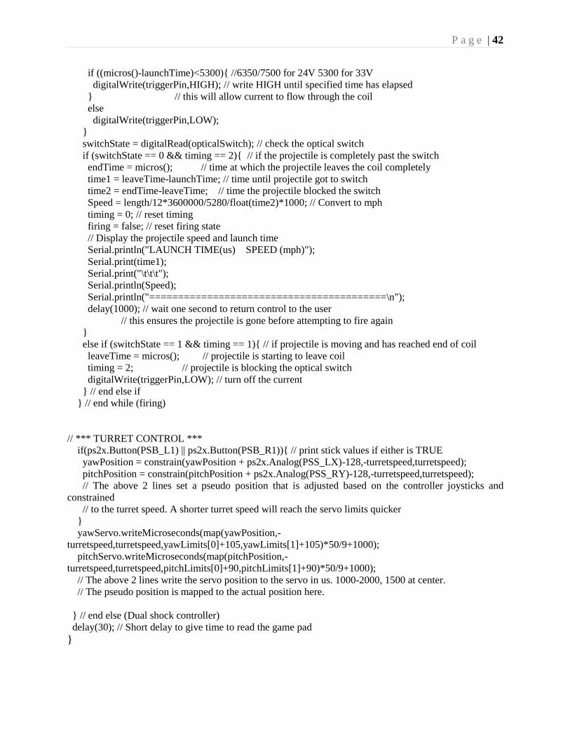
P a g e | 42
if ((micros()-launchTime)<5300) //6350/7500 for 24V 5300 for 33V
digitalWrite(triggerPin,HIGH); // write HIGH until specified time has elapsed
// this will allow current to flow through the coil
else
digitalWrite(triggerPin,LOW);
switchState = digitalRead(opticalSwitch); // check the optical switch
if (switchState == 0 && timing == 2) // if the projectile is completely past the switch
endTime = micros(); // time at which the projectile leaves the coil completely
time1 = leaveTime-launchTime; // time until projectile got to switch
time2 = endTime-leaveTime; // time the projectile blocked the switch
Speed = length/12*3600000/5280/float(time2)*1000; // Convert to mph
timing = 0; // reset timing
firing = false; // reset firing state
// Display the projectile speed and launch time
Serial.println("LAUNCH TIME(us) SPEED (mph)");
Serial.print(time1);
Serial.print("\t\t\t");
Serial.println(Speed);
Serial.println("=========================================\n");
delay(1000); // wait one second to return control to the user
// this ensures the projectile is gone before attempting to fire again
else if (switchState == 1 && timing == 1) // if projectile is moving and has reached end of coil
leaveTime = micros(); // projectile is starting to leave coil
timing = 2; // projectile is blocking the optical switch
digitalWrite(triggerPin,LOW); // turn off the current
// end else if
// end while (firing)
// *** TURRET CONTROL ***
if(ps2x.Button(PSB_L1) || ps2x.Button(PSB_R1)) // print stick values if either is TRUE
yawPosition = constrain(yawPosition + ps2x.Analog(PSS_LX)-128,-turretspeed,turretspeed);
pitchPosition = constrain(pitchPosition + ps2x.Analog(PSS_RY)-128,-turretspeed,turretspeed);
// The above 2 lines set a pseudo position that is adjusted based on the controller joysticks and
constrained
// to the turret speed. A shorter turret speed will reach the servo limits quicker
yawServo.writeMicroseconds(map(yawPosition,-
turretspeed,turretspeed,yawLimits[0]+105,yawLimits[1]+105)*50/9+1000);
pitchServo.writeMicroseconds(map(pitchPosition,-
turretspeed,turretspeed,pitchLimits[0]+90,pitchLimits[1]+90)*50/9+1000);
// The above 2 lines write the servo position to the servo in us. 1000-2000, 1500 at center.
// The pseudo position is mapped to the actual position here.
// end else (Dual shock controller)
delay(30); // Short delay to give time to read the game pad

P a g e | 43
A.5 Simulink Models of Coil Gun
Figure A - 6: Simulink Model of Coil Gun With No Flyback Diode
Figure A - 7: Simulink Model of Coil Gun With Flyback Diode Included
I
To Workspace4
time
To Workspace3
VL
To Workspace2
VR
To Workspace1
Vc
To Workspace
R
Resistor
1
s
Integrator1
1
s
Integrator
Clock
1/L
1/L
-K-
1/C
Icap
To Workspace5Icoil
To Workspace4
time
To Workspace3VL
To Workspace2
VR
To Workspace1
Vc
To Workspace
> 0
Switch
R
Resistor
1
s
Integrator1
1
s
Integrator
0 Constant
Clock
1/L
1/L
-K-
1/C
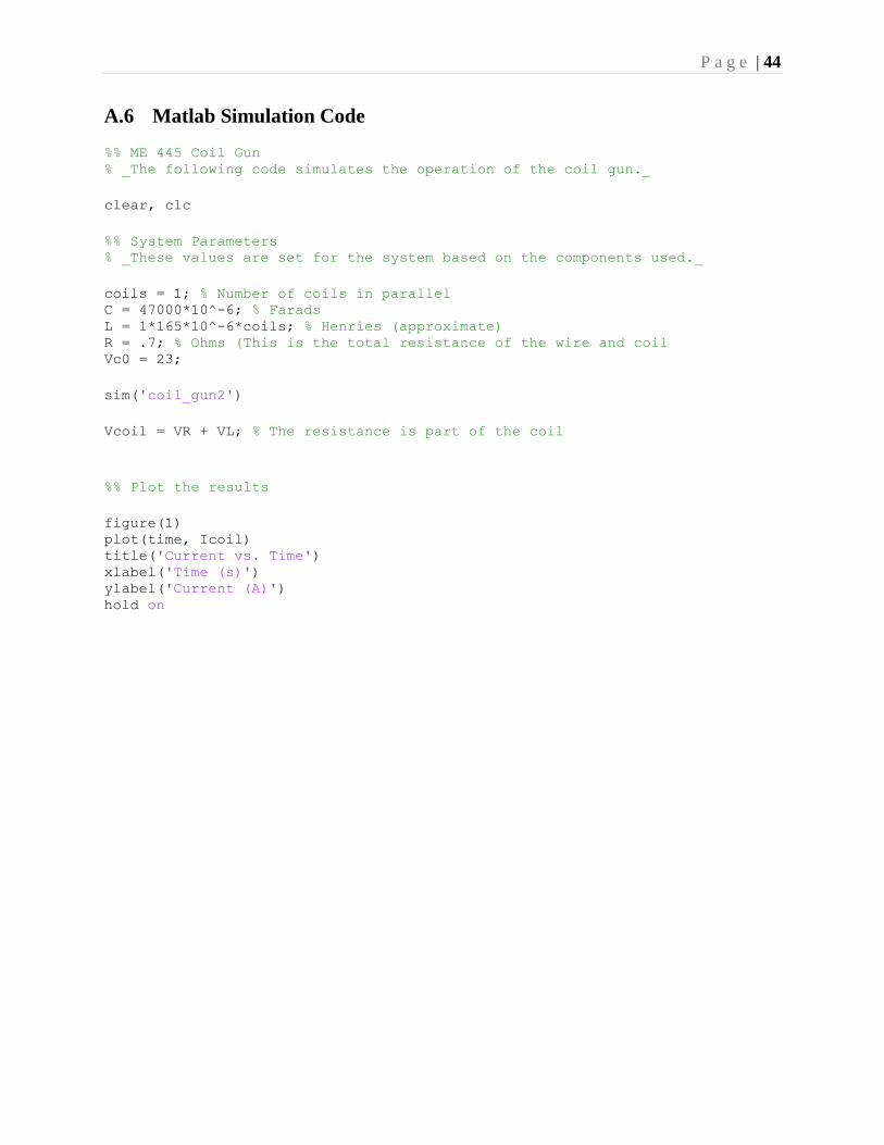
P a g e | 44
A.6 Matlab Simulation Code
%% ME 445 Coil Gun % _The following code simulates the operation of the coil gun._
clear, clc
%% System Parameters % _These values are set for the system based on the components used._
coils = 1; % Number of coils in parallel C = 47000*10^-6; % Farads L = 1*165*10^-6*coils; % Henries (approximate) R = .7; % Ohms (This is the total resistance of the wire and coil Vc0 = 23;
sim('coil_gun2')
Vcoil = VR + VL; % The resistance is part of the coil
%% Plot the results
figure(1) plot(time, Icoil) title('Current vs. Time') xlabel('Time (s)') ylabel('Current (A)') hold on

P a g e | 45
A.7 Matlab Data Gathering Code
% PMD1208_2ch.m - sample one A/D channel on PMD-1208FS % HJSIII, 03.07.29 % Mike Pritts, 05.05.24
% connect MATLAB object (ai) to ComputerBoards (mcc) device (1) % in 339 Reber, the PMD-1208FS boards are installed as mcc device 1 ai = analoginput( 'mcc', 1 );
% use channels 0 addchannel( ai, 0 );
set(ai, 'InputType', 'Differential');
% sampling rate and length of burst set( ai, 'SampleRate', 20000 ) set( ai, 'SamplesPerTrigger', 65536 )
% activate PMD-1208FS - NOTE: this does not actually start sampling start( ai )
% sample burst [ data, time, abstime, events ] = getdata( ai );
% organize data chan0 = data(:,1);
% plot figure(3) plot( time, chan0 ) xlabel( 'Time [sec]' ) ylabel( 'Channel 0 [V]' )
% deactivate board stop(ai);
% deletes board object, ai no longer usable delete(ai) clear ai

Balancing Unicycle Robot ME 445 Final Project
Zack Francis Brian Clough
Spring 2013

1
Contents Introduction ............................................................................................................................................................................... 2
Overall design ........................................................................................................................................................................... 2
Body.......................................................................................................................................................................................... 2
Electronics Shelf and Motor Mounts ........................................................................................................................... 3
Materials ................................................................................................................................................................................. 4
Construction .............................................................................................................................................................................. 4
Hardware .................................................................................................................................................................................... 6
MPU‐6050 .............................................................................................................................................................................. 7
MC33926 Dual Motor Driver ......................................................................................................................................... 7
Software ...................................................................................................................................................................................... 7
Simulation ................................................................................................................................................................................... 8
Testing and Results ................................................................................................................................................................. 9
Discussio ................................................................................................................................................................................... 10
Appendix ................................................................................................................................................................................... 12

2
Introduction Two wheeled balancing robots have been successful in many projects and perhaps most famously in industry with the Segway. The goal of this project was to take that success and go one step further by making it single wheeled. To do this the project would require some design changes from the traditional setup, and require a little more control. The biggest change comes with the addition of a reaction wheel positioned at the top of the robot to compensate for side to side tilting. This functions under the principle of conservation of angular momentum, and is what is used in many aerospace systems to rotate satellites in space. With a general idea in mind, the project progressed to the design of the robot.
Overall design The design of a balancing robot is very important and can determine whether or not a robot is successful. For an inverted pendulum, the pendulum arm should be fairly long. This is because a longer arm falls slower than a short arm. A longer arm gives the robot more time to compensate and return the system to equilibrium. This robot’s height was maximized to around 10 inches because of the dimensions of the materials used. This will be elaborated upon later.
Having the robot be symmetric is important, but its more of an aesthetic requirement that a functional one. If a balancing robot isn’t symmetric it can still balance but will look like its tilting or going to fall. All that matters is the center of gravity is over the axel of the bottom wheels.
Body The body and structural features of the robot were all made out of quarter inch acrylic plastic. The body consisted of two identical sides roughly 11x6 inches, an electronics shelf of 2x3 inches and two motor mounts of one inch square each. The sides consisted of a rounded bottom with three holes for the bottom motor to be mounted to from the outside. The end was rounded and narrowed down for easier access to the motor and wheel.
Directly in the center of the side plate there is a hole that served several purposes. One was to act as a way for the motor wires to reach the Arduino on the inside of the robot. Another purpose was to give the group easier access to the wires and electronics on the inside. The hole was large enough for a finger to go in and adjust a wire that might have been knocked loose.
At the top of the side plate there is a vertical slot about one inch wide. This slot is for the upper reaction wheel. A motor would be mounted parallel to the plane of the side plate and the reaction wheel would be help perpendicular to that plane; spinning within the slot. With the motor mounted as high as possible, the slot allowed for a six inch reaction wheel.
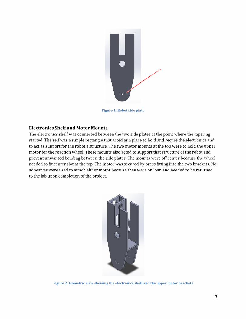
3
Figure 1: Robot side plate
Electronics Shelf and Motor Mounts The electronics shelf was connected between the two side plates at the point where the tapering started. The self was a simple rectangle that acted as a place to hold and secure the electronics and to act as support for the robot’s structure. The two motor mounts at the top were to hold the upper motor for the reaction wheel. These mounts also acted to support that structure of the robot and prevent unwanted bending between the side plates. The mounts were off center because the wheel needed to fit center slot at the top. The motor was secured by press fitting into the two brackets. No adhesives were used to attach either motor because they were on loan and needed to be returned to the lab upon completion of the project.
Figure 2: Isometric view showing the electronics shelf and the upper motor brackets

4
Materials The design of the robot was dictated partially by the materials that were supplied to group at the start of the project. A one foot square piece of acrylic plastic was available so the maximum dimensions of the robot were limited to one foot. For simplifies sake the whole main body was designed to be made out of the acrylic. This included the two sides, the shelf for the electronics and the upper motor mounts.
Table 1: Project bill of materials
Construction Once the body and structural components where designed in SolidWorks, they were placed into a SolidWorks drawing and sent to the laser cutter. The drawing needed to be saved as a .dxf file so it would be compatible with the cutter’s software. The laser cutter cuts any lines that are in the .dxf file so all dimensions, construction lines and title block needed to be removed. The laser cutter took only a few minutes to complete cutting out the pieces from the acrylic sheet.
Figure 3: Image of the parts as they were to be cut
Once the body components were cut, they needed to be assembled into the desired structure. During the process of considering how to assemble the pieces, some mistakes in the design where
Item Quantity Cost
34:1 Pololu metal gearmotor 2 $73.90
Wheel 1 $9.95
Reaction Wheel (Wooden disc and four
1 oz. weights) 1 $3.00
MPU‐6050 Accelerometer/Gyro 1 $39.95
Acrylic 1ftx1ft $8.18
MC33926 Pololu motor driver 1 $29.95
Total Cost $164.93
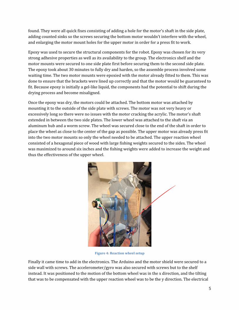
5
found. They were all quick fixes consisting of adding a hole for the motor’s shaft in the side plate, adding counted sinks so the screws securing the bottom motor wouldn’t interfere with the wheel, and enlarging the motor mount holes for the upper motor in order for a press fit to work.
Epoxy was used to secure the structural components for the robot. Epoxy was chosen for its very strong adhesive properties as well as its availability to the group. The electronics shelf and the motor mounts were secured to one side plate first before securing them to the second side plate. The epoxy took about 30 minutes to fully dry and harden, so the assemble process involved some waiting time. The two motor mounts were epoxied with the motor already fitted to them. This was done to ensure that the brackets were lined up correctly and that the motor would be guaranteed to fit. Because epoxy is initially a gel‐like liquid, the components had the potential to shift during the drying process and become misaligned.
Once the epoxy was dry, the motors could be attached. The bottom motor was attached by mounting it to the outside of the side plate with screws. The motor was not very heavy or excessively long so there were no issues with the motor cracking the acrylic. The motor’s shaft extended in between the two side plates. The lower wheel was attached to the shaft via an aluminum hub and a worm screw. The wheel was secured close to the end of the shaft in order to place the wheel as close to the center of the gap as possible. The upper motor was already press fit into the two motor mounts so only the wheel needed to be attached. The upper reaction wheel consisted of a hexagonal piece of wood with large fishing weights secured to the sides. The wheel was maximized to around six inches and the fishing weights were added to increase the weight and thus the effectiveness of the upper wheel.
Figure 4: Reaction wheel setup
Finally it came time to add in the electronics. The Arduino and the motor shield were secured to a side wall with screws. The accelerometer/gyro was also secured with screws but to the shelf instead. It was positioned to the motion of the bottom wheel was in the x direction, and the tilting that was to be compensated with the upper reaction wheel was to be the y direction. The electrical

componeany wire plate fromon the ro
HardwThe electrobot; an7.2V battbrought t
ents were secdisconnectiom the lower mbot and to ba
ware tronics setupn Arduino, MPtery. Figure 4together.
cured with scons due to shmotor and thalance out th
p consisted ofPU‐6050 acc4 below show
crews so theyhifting. The 7he Arduino. The weight fro
Figure 5
f six main coelerometer/ws the circuit
Figure 6: C
y could be re7.2V battery wThis was to som the other
: Assembled ro
mponents thgyro, MC339t configuratio
Circuit configur
emovable butwas attachedhift the shiftcomponents
obot
hat worked to926 motor dron, and how
ration
t rigid enougd high on thet the center os.
ogether to trriver, two DCthe compone
gh to elimina opposite sidof gravity hig
ry and balancC motors, andents were
6
ate de gher
ce the d a

7
The MC33926 motor driver doubled as a shield for the Arduino, and the Arduino/MC33926 combination served as the base to which the other components were connected.
MPU6050 The MPU‐6050 accelerometer/gyroscope came on the SEN‐11028 breakout board from Sparkfun which made it easy to use the six pins used in this project. The chip communicated to the Arduino via the SCL and SDA lines on analog pins five and four respectively. The chip was powered with 3.3 volts and also utilized the Arduino digital pin two for an interrupt in the case that there were any errors in the chip setup. The MPU‐6050 could have one of two addresses, 1101001 or 1101000. The final bit in the address was determined by pin AD0 and was tied to VDD by default on the SEN‐11028 board making the address used in the project 1101001 or 69 in Hexadecimal.
MC33926 Dual Motor Driver The motor driver fit directly on top of the Arduino as seen on the right, and was able to perform a variety of functions. It had the ability to control two DC motors in both speed and direction. Much like the Pololu motor driver used previously in the semester, there was a pin for direction and another used with PWM to control speed for each motor. The MC33926 also performed another function by outputting the current being used by each motor to analog pins zero and one. The battery was hooked up to VIN and GND of the motor driver, and the driver was able to then power the Arduino without the connection of the USB cable.
Software The first priority for programming was being able to read data from the accelerometer/gyro. An attempt at a custom program was made by using various I2C commands from the wire library of Arduino. This proved unsuccessful, and code found on github.com was used which provided angle readings. This new code required a few additional libraries to help calculate the angle readings from the sensor and provided a few other functions which remained unused. The second task was to develop controls to balance the robot in each direction. For this, a PID (Proportion, Integral, Derivative) controller was implemented. Initial values for the controllers were found using the simulations described below. The final version of the Arduino program can be found in the appendix.

8
Simulation To better understand how the robot would react, a simulation of the robot in both directions was created in VisSim. This consisted of three state equations; one for the angle of the robot in the direction of movement, one for the movement itself, and the third for the angle of the robot perpendicular to the direction of movement. Equation 1 below solves for the angular acceleration of the robot in the direction of motion. This was modeled as an inverted pendulum on a moving base.
(1)
T represents the motor output torque, r is the radius of the wheel, M is the mass of the wheel assembly, m is the mass of the rest of the robot, and l is the distance from the axel to the robot’s center of gravity. The second equation (Eq. 2) of motion finds the robots acceleration forward from its angle and angular acceleration.
(2)
The final equation of motion is used for the robot’s angle side to side, or perpendicular to the direction of motion. Unlike in the direction of motion, the robot in this direction was modeled as an inverted pendulum with a stationary base.
(3)
In Eq. 3, m2 represents the mass of the entire robot, l2 represents distance from the base of the robot to its center of gravity, I2 represents the inertia of the robot, and T2 is the torque outputted by the motor on the reaction wheel.
Since the motors were not controlled simply by inputted a specific torque, the motors themselves had to be analyzed. Equation 4 shows the relationship between torque and voltage using constants (kt and kv), motor speed (ω), and motor resistance (Rmotor).
(4)
To find kt and kv, equations 5 and 6 were used with specs for the motor. Kt and kv were found to have a value of 0.0707.
(5)
(6)
Three PID controllers were added into the simulation to balance the robot in each direction and to control the distance traveled. These values were tuned in the simulation and then used as a starting point for the tuning of the actual robot. To ensure that the simulation was relatable to the actual

robot, limand 8.
TestingOnce the propertiemass wasaxel. The inertia wthe oscillthe momeconstants
Once the control bin the balIn order talone, an
mits were pla
Fig
Figure 8:
g and Resrobot was ases were calcus estimated by position ofas determineation. By coment of inertias in the PID c
software waegan. Modelill park of whto help reducd then the up
aced on the v
ure 7: Angle re
Response in th
sults ssembled, thulated initiallby balancing f the center oed by flippinmbining the wa of the robotcontrol.
as uploaded ting the systeere they shoce the amounpper wheel w
oltages. Simu
esponse of the
he direction of
he testing andly. The mass the robot onof gravity wag the robot uweight, distat was calcula
to the Arduinem to determuld be. It taknt of variablewas tested al
ulations of th
e system startin
f motion when
d troubleshowas determn a fulcrum aas assumed toupside downance to the ceated. These v
no, testing tomine prime cokes hours of mes to consideone.
he system are
ng 0.05 radian
n starting 0.05
ot phase of tined using a nd measurino be in the ce and measurenter of gravvalues were u
o determine bonstants is heminor tweaker at once, the
e shown belo
ns off balance
radians off bal
he project bescale in the lng the distancenter of the rring the naturity and the nused to deter
best constantelpful but canking to get thee bottom wh
ow in Figure
lance
egan. Some inlab. The centce from the lrobot. The roral frequencynatural frequrmine the
ts for the PIDn only get the constants cheel was teste
9
s 7
nitial ter of lower obot’s y of ency,
D em close. ed

10
Attempting to improve the balance of the robot proved to be a difficult task, one that involved a lot of educated guess work. Once the constants were set to be in the ball park, it was just a matter of increasing or decreasing them one at a time to attempt to get them close to the right values. The proportional constant tends to make the system react faster but also increased the tendency for over‐shooting the desired position. The integrator constant tends to increase damping, thus lowering over‐shoot but can affect the system negatively if set too high. The derivative constant could be used to try and reduce the chatter of the system, but like the integrator, could also cause major stability problems if out or proportion with the other constants.
Testing of the lower wheel took the most time of the two wheels. In order to prevent the robot from tipping in the y direction, a second wheel was added to the bottom. Initially the second wheel was added in between the two side plates, but this proved to be a little unstable. Although testing was still conducted on this arrangement, the extra wheel was moved to the outside of the robot to increase stability later in the testing process.
Testing of the upper wheel proved to be the most challenging and ambitious part of the project. To isolate the upper wheel, the bottom wheel was fixed to prevent it from moving. This affectively made the robot a fixed inverted pendulum. The group didn’t have much experience with using reaction wheels. The extent of the experience was some physics behind how it worked and a few videos online showing that it could work. After some brief initial testing, it became apparent that the wheel was not sized correctly. There was not nearly enough inertia being generated to compensate for and angle error of more than a few tenths of a degree. It is not realistic to assume a homemade robot can keep itself within a tenth of a degree from vertical. Even computer model of the system was only stable within a few degrees. Because of the difficulty the reaction wheel presented, the project was modified to only involve the lower wheel. The second wheel on the bottom was made a permanent design feature and the upper wheel was removed.
After hours of tweaking the three constants for the PID control, the robot was only marginally successful at maintaining its balance. Under the best circumstances, the robot would start off fairly stable for a second or so. Then the system would start becoming unstable as the robot started rocking back and forth. The increasing magnitude of the acceleration made the system become completely unstable and the robot would not be able to adjust to return to equilibrium. The test would conclude with the robot driving in one direction with the wheel trying in vain to catch up with its upper half. The robot would have hit the ground if it wasn’t caught by a group member. Luckily the robots best display of balance was caught on video. It balanced for around 5 seconds before reaching an angle it couldn’t recover from.
Discussion
There were several issues that were revealed over the duration for the project. Some of the earlier issues were in regards to the robot design. Initially the upper motor was press fitted into the two motor brackets. This was a poor design because it became incredibly hard to remove the motor for replacement. Excessive torque on the motor broke a few teeth off of one of the internal gears,

11
rendering the motor unusable. It took a lot of unnecessary effort to remove the broken motor, and the body of the robot broke in the process. A future design would include a fixture similar to the lower wheel and have a loose fitting bracket in the back of the motor for added support.
In regards to the overall assembly of the robot, epoxy was a poor choice to use to secure the parts. One the epoxy was set, there wasn’t an easy way to modify the design or take the robot apart without breaking it. Luckily the epoxy was always the first thing to break, but then the parts needed to be re‐epoxied and left for 30 minutes to harden. A future design would utilize small screws to secure all the parts in place. Although this would add effort to be sure the holes lined up perfectly, the benefit of being able to take apart the robot easily would make it worth it.
Another issue the robot had was from the gyro and accelerometer sensor. The sensor was very accurate but had a substantial angle drift. With our software to prevent this drift, the measured angular position of the robot would change several tenths of a degree even when held stationary. This posed a huge problem for balancing because after a few seconds, the robot would be trying to reach an equilibrium that corresponded to an unstable position. In other words, the robot would lose any hope of balancing after only a few seconds. This problem was alleviated with the help of some more sophisticated code taken off the internet. The code took a running average of the angle measurement to help maintain the correct angle for equilibrium.
In hindsight, it is quite apparent that this project was too ambitious and beyond the scope of this class. It was brought to the attention of the group that a PID controller was probably not robust enough to control a balancing robot, much less a unicycle robot. This project essentially combines two separate projects into one; a balancing robot with a moving base and an inverted pendulum with a stationary base. Each one of these could have been a project in itself, but combining them made it nearly impossible to complete in the timeframe and budget we were given. In order to have a greater chance at success, the robot would need to be completely redesigned, without the restrictions of material that the current design had.
This project was incredibly exciting to work on. Being able to plan, design, build, program and test a robot from scratch was a great feeling. Even having the ability to choose our own project made this project great. This project involved learning how to use unfamiliar electronics, unfamiliar hardware and unfamiliar and difficult software. The members of this group had to spend many hours researching how the code worked and what the right configuration for the hardware should be. This was a very rewarding project, even though the robot only achieved marginal success. The things learned over the course of this project have spurred a new a newfound interest that will probably become a hobby in the future; mechatronics.

12
Appendix #include <DualMC33926MotorShield.h> // I2C device class (I2Cdev) demonstration Arduino sketch for MPU6050 class using DMP (MotionApps v2.0) // 6/21/2012 by Jeff Rowberg <[email protected]> // Updates should (hopefully) always be available at https://github.com/jrowberg/i2cdevlib // // Changelog: // 2012‐06‐21 ‐ added note about Arduino 1.0.1 + Leonardo compatibility error // 2012‐06‐20 ‐ improved FIFO overflow handling and simplified read process // 2012‐06‐19 ‐ completely rearranged DMP initialization code and simplification // 2012‐06‐13 ‐ pull gyro and accel data from FIFO packet instead of reading directly // 2012‐06‐09 ‐ fix broken FIFO read sequence and change interrupt detection to RISING // 2012‐06‐05 ‐ add gravity‐compensated initial reference frame acceleration output // ‐ add 3D math helper file to DMP6 example sketch // ‐ add Euler output and Yaw/Pitch/Roll output formats // 2012‐06‐04 ‐ remove accel offset clearing for better results (thanks Sungon Lee) // 2012‐06‐01 ‐ fixed gyro sensitivity to be 2000 deg/sec instead of 250 // 2012‐05‐30 ‐ basic DMP initialization working /* ============================================ I2Cdev device library code is placed under the MIT license Copyright (c) 2012 Jeff Rowberg Permission is hereby granted, free of charge, to any person obtaining a copy of this software and associated documentation files (the "Software"), to deal in the Software without restriction, including without limitation the rights to use, copy, modify, merge, publish, distribute, sublicense, and/or sell copies of the Software, and to permit persons to whom the Software is furnished to do so, subject to the following conditions: The above copyright notice and this permission notice shall be included in all copies or substantial portions of the Software. THE SOFTWARE IS PROVIDED "AS IS", WITHOUT WARRANTY OF ANY KIND, EXPRESS OR IMPLIED, INCLUDING BUT NOT LIMITED TO THE WARRANTIES OF MERCHANTABILITY, FITNESS FOR A PARTICULAR PURPOSE AND NONINFRINGEMENT. IN NO EVENT SHALL THE AUTHORS OR COPYRIGHT HOLDERS BE LIABLE FOR ANY CLAIM, DAMAGES OR OTHER LIABILITY, WHETHER IN AN ACTION OF CONTRACT, TORT OR OTHERWISE, ARISING FROM, OUT OF OR IN CONNECTION WITH THE SOFTWARE OR THE USE OR OTHER DEALINGS IN THE SOFTWARE. =============================================== */ // Arduino Wire library is required if I2Cdev I2CDEV_ARDUINO_WIRE implementation // is used in I2Cdev.h #include "Wire.h" // I2Cdev and MPU6050 must be installed as libraries, or else the .cpp/.h files // for both classes must be in the include path of your project #include "I2Cdev.h" #include "MPU6050_6Axis_MotionApps20.h" #include "MPU6050.h" // not necessary if using MotionApps include file
13
#include "helper_3dmath.h" // class default I2C address is 0x68 // specific I2C addresses may be passed as a parameter here // AD0 low = 0x68 (default for SparkFun breakout and InvenSense evaluation board) // AD0 high = 0x69 float dt, time, time2; float gyrox, accelx, anglex, gyroy, accely, angley, error1, error3, deriv2, integral2, error0, error2, deriv, integral; int kp1=400, ki1=65, kd1=15, x_val=0, x_filt, out, kp2=150, ki2=5, kd2=15, out2; DualMC33926MotorShield md; MPU6050 mpu; /* ========================================================================= NOTE: In addition to connection 3.3v, GND, SDA, and SCL, this sketch depends on the MPU‐6050's INT pin being connected to the Arduino's external interrupt #0 pin. On the Arduino Uno and Mega 2560, this is digital I/O pin 2. * ========================================================================= */ /* ========================================================================= NOTE: Arduino v1.0.1 with the Leonardo board generates a compile error when using Serial.write(buf, len). The Teapot output uses this method. The solution requires a modification to the Arduino USBAPI.h file, which is fortunately simple, but annoying. This will be fixed in the next IDE release. For more info, see these links: http://arduino.cc/forum/index.php/topic,109987.0.html http://code.google.com/p/arduino/issues/detail?id=958 * ========================================================================= */ // uncomment "OUTPUT_READABLE_QUATERNION" if you want to see the actual // quaternion components in a [w, x, y, z] format (not best for parsing // on a remote host such as Processing or something though) //#define OUTPUT_READABLE_QUATERNION // uncomment "OUTPUT_READABLE_EULER" if you want to see Euler angles // (in degrees) calculated from the quaternions coming from the FIFO. // Note that Euler angles suffer from gimbal lock (for more info, see // http://en.wikipedia.org/wiki/Gimbal_lock) #define OUTPUT_READABLE_EULER // uncomment "OUTPUT_READABLE_YAWPITCHROLL" if you want to see the yaw/ // pitch/roll angles (in degrees) calculated from the quaternions coming // from the FIFO. Note this also requires gravity vector calculations. // Also note that yaw/pitch/roll angles suffer from gimbal lock (for // more info, see: http://en.wikipedia.org/wiki/Gimbal_lock) //#define OUTPUT_READABLE_YAWPITCHROLL // uncomment "OUTPUT_READABLE_REALACCEL" if you want to see acceleration // components with gravity removed. This acceleration reference frame is
14
// not compensated for orientation, so +X is always +X according to the // sensor, just without the effects of gravity. If you want acceleration // compensated for orientation, us OUTPUT_READABLE_WORLDACCEL instead. //#define OUTPUT_READABLE_REALACCEL // uncomment "OUTPUT_READABLE_WORLDACCEL" if you want to see acceleration // components with gravity removed and adjusted for the world frame of // reference (yaw is relative to initial orientation, since no magnetometer // is present in this case). Could be quite handy in some cases. //#define OUTPUT_READABLE_WORLDACCEL // uncomment "OUTPUT_TEAPOT" if you want output that matches the // format used for the InvenSense teapot demo #define OUTPUT_TEAPOT #define LED_PIN 13 // (Arduino is 13, Teensy is 11, Teensy++ is 6) bool blinkState = false; // MPU control/status vars bool dmpReady = false; // set true if DMP init was successful uint8_t mpuIntStatus; // holds actual interrupt status byte from MPU uint8_t devStatus; // return status after each device operation (0 = success, !0 = error) uint16_t packetSize; // expected DMP packet size (default is 42 bytes) uint16_t fifoCount; // count of all bytes currently in FIFO uint8_t fifoBuffer[64]; // FIFO storage buffer // orientation/motion vars Quaternion q; // [w, x, y, z] quaternion container VectorInt16 aa; // [x, y, z] accel sensor measurements VectorInt16 aaReal; // [x, y, z] gravity‐free accel sensor measurements VectorInt16 aaWorld; // [x, y, z] world‐frame accel sensor measurements VectorFloat gravity; // [x, y, z] gravity vector float euler[3]; // [psi, theta, phi] Euler angle container float ypr[3]; // [yaw, pitch, roll] yaw/pitch/roll container and gravity vector // packet structure for InvenSense teapot demo uint8_t teapotPacket[14] = '$', 0x02, 0,0, 0,0, 0,0, 0,0, 0x00, 0x00, '\r', '\n' ; // ================================================================ // === INTERRUPT DETECTION ROUTINE === // ================================================================ volatile bool mpuInterrupt = false; // indicates whether MPU interrupt pin has gone high void dmpDataReady() mpuInterrupt = true; // ================================================================ // === INITIAL SETUP ===

15
// ================================================================ void setup() // join I2C bus (I2Cdev library doesn't do this automatically) Wire.begin(); md.init(); // initialize serial communication // (115200 chosen because it is required for Teapot Demo output, but it's // really up to you depending on your project) Serial.begin(115200); while (!Serial); // wait for Leonardo enumeration, others continue immediately // NOTE: 8MHz or slower host processors, like the Teensy @ 3.3v or Ardunio // Pro Mini running at 3.3v, cannot handle this baud rate reliably due to // the baud timing being too misaligned with processor ticks. You must use // 38400 or slower in these cases, or use some kind of external separate // crystal solution for the UART timer. // initialize device Serial.println(F("Initializing I2C devices...")); mpu.initialize(); // verify connection Serial.println(F("Testing device connections...")); Serial.println(mpu.testConnection() ? F("MPU6050 connection successful") : F("MPU6050 connection failed")); // wait for ready Serial.println(F("\nSend any character to begin DMP programming and demo: ")); //while (Serial.available() && Serial.read()); // empty buffer //while (!Serial.available()); // wait for data //while (Serial.available() && Serial.read()); // empty buffer again // load and configure the DMP Serial.println(F("Initializing DMP...")); devStatus = mpu.dmpInitialize(); // make sure it worked (returns 0 if so) if (devStatus == 0) // turn on the DMP, now that it's ready Serial.println(F("Enabling DMP...")); mpu.setDMPEnabled(true); // enable Arduino interrupt detection Serial.println(F("Enabling interrupt detection (Arduino external interrupt 0)...")); attachInterrupt(0, dmpDataReady, RISING); mpuIntStatus = mpu.getIntStatus(); // set our DMP Ready flag so the main loop() function knows it's okay to use it Serial.println(F("DMP ready! Waiting for first interrupt...")); dmpReady = true; // get expected DMP packet size for later comparison packetSize = mpu.dmpGetFIFOPacketSize(); else

16
// ERROR! // 1 = initial memory load failed // 2 = DMP configuration updates failed // (if it's going to break, usually the code will be 1) Serial.print(F("DMP Initialization failed (code ")); Serial.print(devStatus); Serial.println(F(")")); // configure LED for output pinMode(LED_PIN, OUTPUT); // ================================================================ // === MAIN PROGRAM LOOP === // ================================================================ void loop() // if programming failed, don't try to do anything if (!dmpReady) return; // wait for MPU interrupt or extra packet(s) available while (!mpuInterrupt && fifoCount < packetSize) // other program behavior stuff here // . // . // . // if you are really paranoid you can frequently test in between other // stuff to see if mpuInterrupt is true, and if so, "break;" from the // while() loop to immediately process the MPU data // . // . // . // reset interrupt flag and get INT_STATUS byte mpuInterrupt = false; mpuIntStatus = mpu.getIntStatus(); // get current FIFO count fifoCount = mpu.getFIFOCount(); // check for overflow (this should never happen unless our code is too inefficient) if ((mpuIntStatus & 0x10) || fifoCount == 1024) // reset so we can continue cleanly mpu.resetFIFO(); // Serial.println(F("FIFO overflow!")); // otherwise, check for DMP data ready interrupt (this should happen frequently) else if (mpuIntStatus & 0x02) // wait for correct available data length, should be a VERY short wait while (fifoCount < packetSize) fifoCount = mpu.getFIFOCount();

17
// read a packet from FIFO mpu.getFIFOBytes(fifoBuffer, packetSize); // track FIFO count here in case there is > 1 packet available // (this lets us immediately read more without waiting for an interrupt) fifoCount ‐= packetSize; #ifdef OUTPUT_READABLE_QUATERNION // display quaternion values in easy matrix form: w x y z mpu.dmpGetQuaternion(&q, fifoBuffer); /* Serial.print("quat\t"); Serial.print(q.w); Serial.print("\t"); Serial.print(q.x); Serial.print("\t"); Serial.print(q.y); Serial.print("\t"); Serial.println(q.z);*/ #endif #ifdef OUTPUT_READABLE_EULER // display Euler angles in degrees mpu.dmpGetQuaternion(&q, fifoBuffer); mpu.dmpGetEuler(euler, &q); // Serial.print("euler\t"); Serial.println(error1) ;//* 180/M_PI); //Serial.print("\t"); //Serial.print(euler[1]) ;//* 180/M_PI); //Serial.print("\t"); //Serial.println(euler[2]); //* 180/M_PI); #endif //********************************************************************************************************** //********************************************************************************************************** //PID Controller and filter //time=micros()/1000000; dt=.01; anglex=euler[1]; angley=euler[2]; time=micros()/1000000; error0=(0‐anglex)*20; deriv=kd1*(error0‐error2)/dt; integral+=(error0*dt)*ki1; out=(kp1*error0+integral+deriv)*1000; //md.setM1Speed(out); error2=error0; time2=time; // error1=(0.04‐angley)*2; deriv2=kd2*(error1‐error3)/dt; integral2+=ki2*(error1*dt);

18
out2=(kp2*error1+integral2+deriv2)*‐25; md.setM2Speed(out2); error3=error1; //Serial.println(anglex, DEC); //delay(5); //********************************************************************************************************** //********************************************************************************************************** #ifdef OUTPUT_READABLE_YAWPITCHROLL // display Euler angles in degrees mpu.dmpGetQuaternion(&q, fifoBuffer); mpu.dmpGetGravity(&gravity, &q); mpu.dmpGetYawPitchRoll(ypr, &q, &gravity); /* Serial.print("ypr\t"); Serial.print(ypr[0] * 180/M_PI); Serial.print("\t"); Serial.print(ypr[1] * 180/M_PI); Serial.print("\t"); Serial.println(ypr[2] * 180/M_PI);*/ #endif #ifdef OUTPUT_READABLE_REALACCEL // display real acceleration, adjusted to remove gravity mpu.dmpGetQuaternion(&q, fifoBuffer); mpu.dmpGetAccel(&aa, fifoBuffer); mpu.dmpGetGravity(&gravity, &q); mpu.dmpGetLinearAccel(&aaReal, &aa, &gravity); /* Serial.print("areal\t"); Serial.print(aaReal.x); Serial.print("\t"); Serial.print(aaReal.y); Serial.print("\t"); Serial.println(aaReal.z);*/ #endif #ifdef OUTPUT_READABLE_WORLDACCEL // display initial world‐frame acceleration, adjusted to remove gravity // and rotated based on known orientation from quaternion mpu.dmpGetQuaternion(&q, fifoBuffer); mpu.dmpGetAccel(&aa, fifoBuffer); mpu.dmpGetGravity(&gravity, &q); mpu.dmpGetLinearAccel(&aaReal, &aa, &gravity); mpu.dmpGetLinearAccelInWorld(&aaWorld, &aaReal, &q); /* Serial.print("aworld\t"); Serial.print(aaWorld.x); Serial.print("\t"); Serial.print(aaWorld.y); Serial.print("\t"); Serial.println(aaWorld.z);*/ #endif #ifdef OUTPUT_TEAPOT // display quaternion values in InvenSense Teapot demo format: teapotPacket[2] = fifoBuffer[0];

19
teapotPacket[3] = fifoBuffer[1]; teapotPacket[4] = fifoBuffer[4]; teapotPacket[5] = fifoBuffer[5]; teapotPacket[6] = fifoBuffer[8]; teapotPacket[7] = fifoBuffer[9]; teapotPacket[8] = fifoBuffer[12]; teapotPacket[9] = fifoBuffer[13]; //Serial.write(teapotPacket, 14); teapotPacket[11]++; // packetCount, loops at 0xFF on purpose #endif //delay(100); // blink LED to indicate activity blinkState = !blinkState; digitalWrite(LED_PIN, blinkState);

Automatic Turret
Shane Rowan and Nicholas Corey
ME 445 – Dr. Sommer
3 MAY 2012

1
Table of Contents
1. Objective………………………………………………………………………………………………..2 2. Approach………………………………………………………………………………………………..2 3. Procedure……………………………………………………………………………………………….3 4. Lessons Learned………………………………………………………………………………………4 5. Suggestions for Future Work…………………………………………………………………..6 6. Results and Conclusion…………………………………………………………………………..7 7. Appendix………………………………………………………………………………………………..8
a. Appendix A – Figures………………………………………………………………..…..8 b. Appendix B – Coding………………………………………………………………..…..9 c. Appendix C – Circuit Diagrams …………………………………………………...13 d. Appendix D – Data Sheets……………………………..…………………………….15

2
Objective:
The automatic turret uses a turntable with an IR sensor attached that is able to track a moving
target and then commence firing at the target. It is also can map a 360 degree view of its
surroundings using the IR sensor.
Approach:
In order to create an automatic turret the system must gather data about the surrounding
environment creating a digital picture. It then will use logic to figure out the closest target and
aim a Nerf gun to shoot at the target. We chose to use a large rotating base that can rotate
similar to a “Lazy-Susan”. This will allow the gun to point in all directions. In order for the
system to gather data about the surroundings we chose an IR sensor. It would rotate at a
constant velocity to determine the coordinates of data points. In order to determine the rate
that the motor was rotating we used a hall sensor that will clock every time the system passes a
magnet on the base. This allows us to create a timing sensor to accurately acquire data from
the sensor. This creates a LIDAR (Laser Infrared Direction and Ranging) system that can
accurately plot the surroundings. By using an IR sensor that rotates at a constant velocity faster
than the base it has the ability to track moving targets, adjusting dynamically.
The next component after the LIDAR is the rotating base that would take inputs from the LIDAR
to face the target. It will face the target and continue to get data inputs to dynamically control
its position to accurately aim with respect to angle. The IR sensor is also mapping distance and
which will be used to determine the angle of fire of the cannon.
The final component of our design is the cannon. It must be able to load and fire
automatically. We choose to use a modified Nerf gun as the base of the cannon. The Nerf gun
requires air pressure to shoot and would be charged with a motor that will use a pivot arm
similar to a piston in a combustion engine. This converts the rotational motion of the motor to
linear motion successfully pressurizing the gun.
There are many complexities in this problem. The automatic turret requires accurate inputs in
order to rotate to the proper angle. In also must be able to dynamically adjust to the proper
position using continued inputs from the LIDAR. All systems must communicate with respect to
the same coordinate system.

3
Procedure:
This project has three main components that need to be integrated: the LIDAR, the “Lazy -
Susan” orientation system, and the projectile angle adjusting system. Each system while
working simultaneously will identify, track, and fire a projectile at a target.
LIDAR:
The LIDAR system is comprised of three major parts: an infrared detection sensor, a DC motor,
and a Hall Effect sensor. A wire slip ring is attached to a gear which will be driven by the DC
motor. The infrared sensor and the hall sensor are fixed to the top of this gear. As the motor is
powered, the infrared and the hall sensor will rotate continuously in one direction with a
constant angular velocity. Two magnets were fixed offset from the base of the slip ring gear to
allow the Hall sensor to take readings at certain positions 180 degree intervals.
As the LIDAR system operates, the infrared sensor rotates 360 degrees and takes discrete
distance measurements of the surroundings. The number of data points acquired is dependent
upon the speed the DC motor is driven. The hall sensor is clocked on when the infrared sensor
is pointing directly left of the cannon and clocked off when the infrared sensor is pointing
directly right of the cannon. As the Hall sensor clicks on, the number of data points being
gathered begins counting. This creates 180 degrees of data measurements. The counting will
stop when the Hall sensor clocks off. Since the system is running at a constant velocity, the
number of data points being gathered is also constant. The data points are easily converted to
degrees corresponding to where the infrared is facing. For calculations, we set the first angle
recorded as -90 and the last as +90 degrees which is complimented by the placement of the
clocking magnets for the Hall sensor. The measured distance by the infrared sensor is converted
from an analog reading to distance in centimeters. As the LIDAR rotates, the distance and angle
readings are being calculated. For this project, the target will be at the smallest distance
measured. The smallest distance measured and the angle at which it is measured are the
necessary coordinates needed for the orientation system to adjust.
Orientation System:
The orientation system is comprised of a turntable and a Lego motor with optical encoders. The
turntable is modified with a gear so that as the motor is powered, the turntable will rotate
accordingly.
The motor is controlled with a proportional control system and a Pololu driver. The target angle
for the motor is set to the target angle as measured by the LIDAR. The target angle will change
as the turntable rotates or as the target moves. The system will track the position of the target

4
by resetting the zero position of the turntable periodically. This reset will ensure that the
turntable will continuously attempt to orient itself so that the target is directly in front of the
LIDAR.
Projectile System:
The projectile system is comprised of a modified Nerf gun, a dc motor, a servo, and a solenoid.
The Nerf gun was modified with the DC motor so that as the motor is powered, the attached
rod will move a piston that compresses the air necessary for the projectile to fire. The solenoid,
which is fixed to the cannon, triggers the cannon when the necessary signals are sent. The servo
will adjust the angle of the cannon above horizon depending on the measured distance from
the target. The necessary angle is mapped from 0 to 45 degrees based on the tested projectile
trajectories of the cannon.
Circuit diagrams for each system can be found in Appendix XX.
Lessons Learned:
This project was extremely informative, but the biggest lesson is how complex an accurate
LIDAR system can be to implement. The infrared sensor can accurately determine position
within a couple centimeters when there is no motion. However, when used in the LIDAR
system the sensor must rotate fairly quickly in order to gather data about the surroundings. On
our LIDAR system the IR sensor rotated clockwise. The Hall sensors would clock the IR sensor
readings at 90 degrees counter clockwise and would read for 180 degrees. This created a
picture of half a circle to gather raw data. The Arduino would count every time it would run a
loop in the code. Since the loop is constant and the processor is so fast the count is very
consistent and can be used for timing. Initially we assumed that since the IR sensor is rotating
at constant velocity and we had a constant, consistent count that we could divide 180 degrees
evenly and get an accurate map. This turned out to be incorrect. When we would put a target
directly in front of the system which in our coordinate system would be at 0 degrees the sensor
would measure the angle as a positive number. Upon dissecting our code we found that 70
percent of the measurements were on the left of the 0 axis and only 30 percent on the right.
We believe this is due to a processing delay in the IR sensor itself. Once we took this into
account in the code the LIDAR produced accurate measurements, seen in Figure 1-4. Figure 2 is
the map of the box without any targets. The data was taken with the IR sensor rotating
clockwise. This data is of complete 3 rotations plotted alongside each other. Analyzing the
graph one can see a crude box. In this plot one can see a reasonable amount of noise. Next we
used 3 targets inside the box to show that the LIDAR can also receive data with targets. This is

5
shown in Figure 3 and 4. In Figure 4 one can see 3 large peaks in red where the targets are
picked up. Since these targets are not concise, and there are 3 sets of data the large spikes are
difficult to see. The blue data in Figure 4 is the same plot as Figure 2. This validates that the
red lines are in fact the 3 targets. In both plots there is data that is shown on the plot as being
farther that 100 cm. This is when the IR sensor facing the base structure of the system itself.
Even though the actual distance is only a few centimeters the IR sensor reads it as far away
because of the inefficiencies of the sensor itself. It has a minimum range of about 20 cm; a
complete data curve can be seen in Figure 12. All readings that are from the structure of the
system were discarded using the Hall sensor.
Figure 1: LIDAR test- No Targets Figure 2: LIDAR Test- No Targets Plot
Figure 3: LIDAR Test- With Targets Figure 4: LIDAR Test- With Targets Plot

6
After filtering the LIDAR data the results are fairly consistent measurements of a target
position. There are some jumps due to noise in the IR sensor. These values were then used to
calculate the target angle for the base. When this data was used the Arduino was not
calculating the correct angle. This is due to coding errors. The IR sensor would pick up noise
and would rotate to a position that it could no longer see the target. This proved very difficult
and was never completed.
Since the base could not rotate to the target angle the cannon could not properly aim and fire
the target. The cannon did have an efficient charging method with the piston pump and could
accurately fire at a target if the base would point at the target. Since, the cannon did not
receive accurate target positions the projectile angle using a servo was not incorporated. This
would be incorporated in a final design.
The problems with this design are numerous. This design used only one IR sensor. This would
magnify errors in the sensor. This means that the any noise or incorrect measurements are
hard to identify. If we had utilized 2 sensors on a larger base the Arduino could actually
triangulate the position of the target and would be able to eliminate noise. When the IR sensor
is rotating a constant angular velocity the Arduino can track moving targets. However, when
the IR sensor is rotating it can sometimes have sporadic measurements that are not extremely
accurate. If the IR sensor was fixed to the base and the base rotated to create a map of the
surroundings there would be far less noise. This method would lose the ability to track a
moving target, but would be able to find a target, rotate, and fire accurately.
Suggestions for the Future:
The current hardware is sufficient to accurately determine position of a target. The coding
needs to be worked out to accurately be able to eliminate noise. In order to eliminate noise,
one could either reduce the magnitude of change in the target angle so the base does not try to
rotate to false locations. This would cause the system to only be able to track slow moving
targets and would have to initialize to find the target. Or one could look for large spikes in the
IR sensor analog readings. A large spike would identify a target. Then a corresponding drop in
the reading could actually tell the size of the target. The code could then determine the center
of the target.
Another method, briefly explained in the Lessons Learned section is to use 2 IR sensors to
triangulate position. This would really help eliminate any inaccuracies that one sensor would
pick up on. This would create a very accurate map of the surroundings.

7
Results and Conclusion:
For the final prototype, the LIDAR system was able to locate and store the positions of a target.
The LIDAR was able to track the target if the target was moving slowly. The rotating mechanism
was functional but not fully integrated into the entire system. There was an error in the coding
that did not reset the current angle as the turret rotated. The projectile system was also
functional but not fully integrated. The projectile system could automatically recharge the air
pressure, but was unable to load another round. To full integrate this system, the coding would
have to include another section that would adjust the servo to the correct angle, and then fire
the projectile.
This project was very interesting and we learned a lot about LIDAR systems. Our project had a
few flaws that we were unable to fix. If the problems had been debugged in the code the
system would have worked. This was a very difficult project to imagine in the beginning and
now is close to a working automatic turret. This project brought many factors together such as:
analyzing data, using hall sensors, coordinating multiple axis of rotation, and a charging
mechanism for the cannon. We also learned a lot about microprocessors and coordinating
with multiple subsystems. This project made significant progress

8
Appendix:
Figures:
Figure 5: Firing and Recharge mechanism
Figure 6: Complete system
9
Code:
// Variables for the motor control int EncApin=2; int EncBpin=3; int cwpin=9; int ccwpin=10; int gain= 5; float radian; float degree; float pwm; float target; // Target angle for the motor to go to. float voltage; //Voltage represents the proportional voltage sent to the motor; calculated by position. float t1; // Sets the initial time float t2; // Sets the current time // Variables for the LIDAR float distCm; // Distance converted to centimeters int iRmotorPin= 5; int iRmotorSpeed=100; // Rotational speed of the LIDAR (0-255) int iRpin1 = A0; int iRpin2 = A1; float tick=0; //Timing variable for LIDAR float tock=0; //Timing variable for LIDAR int hallPin= 4; int hallVal; int maxTick=0; //Number of rotations in half rotation float iRdegree; // Tick number where sensor encounters closest distance float distTarget1=0; // distance of closest target float distTarget2; // distance of closest target to send out (maybe redundant). float distCC; // Distance measured by IR (analog reading) float tDegree1; // iRdegree converted to degrees. Calculated each rotation. float tDegree2; // Target angle to send to rotation system (target angle.) int n=8; //scaling factor to remove data points in LIDAR range.

10
void setup() Serial.begin(115200); attachInterrupt(0,increment,CHANGE);
// Calls increment function each time the motor changes position pinMode(EncApin, INPUT); pinMode(EncBpin,INPUT); pinMode(ccwpin,OUTPUT); pinMode(cwpin,OUTPUT); analogWrite(iRmotorPin, iRmotorSpeed); t1=micros(); // Sets time to start void loop() lidar(hallVal); // runs LIDAr function voltage= (((3*tDegree2)- degree)*gain);
// Determines how much voltage to send to the motor based on distance from target. t2=micros(); hallVal=digitalRead(hallPin); rotate(voltage,t2); //Serial.println(count); //dist=analogRead(iRpin); /////////////////////////////////////////////////////////////////// void increment() // This function will be called each time the motor changes position and will track // the position change in degrees. if (digitalRead(EncApin) == digitalRead(EncBpin)) // If both pins read the same value, the motor is running clockwise, degrees are added. degree = (degree +1); else // If both pins read different values, the motor is running counter clockwise, degrees are subtracted. degree = (degree-1); ////////////////////////////////////////////////////////////////////////// float rotate(float voltage, float t2) // rotates the motor to reach target position if (voltage > 5) // Trims calculated voltage to 5, the max output possible. voltage=5; if (voltage <-5) voltage =-5; if (voltage > 0) //Means current location is less than the target angle, must spin clockwise to reach target.

11
digitalWrite(ccwpin,HIGH); // Sets CCW pin to OFF digitalWrite(cwpin,LOW); // Sets CW pin to ON pwm= map(voltage,0,5,0,255); // Determines PWM speed based on voltage analogWrite(ccwpin,pwm); // PWMS CCW Pin to slow the CW rotation as the Voltage drops to 0 if (voltage < 0) //Means current location is more than the target angle, must spin counterclockwise to reach target. voltage= voltage *-1; // Sets the voltage to a positive number for the map function digitalWrite(cwpin,HIGH); // Sets CW pin to OFF digitalWrite(ccwpin,LOW); // Sets CCW pin to ON pwm= map(voltage,0,5,0,255); // Determines PWM speed based on voltage analogWrite(cwpin,pwm); // PWMS CW Pin to slow the CCW rotation as the Voltage drops to 0 //////////////////////////////////////////////////////////////////////////// float lidar(int hallVal) if(hallVal==0) dist=analogRead(iRpin1); //dist2=analogRead(iRpin2); //dist= abs(dist2-dist1); tick++; if(distTarget1 < dist && tick > + maxTick/n && tick < maxTick- maxTick/n) // Conditions point to closest reading on IR sensor. distTarget1= dist; //Stores the closest distance iRdegree= tick; // Stores the closest distance angle. if (hallVal == 1) if (tick >1) maxTick=tick; // stores the number of ticks in 90 180 degrees if (tick == maxTick) distTarget2 = distTarget1; //sets closest position send to projectile. distTarget1=0; // resets closest position to be recalculated. count++; //distCC=9462/(distTarget2-16.92)+13; // Converts analog IR reading to centimeter. //distCm = 0.7* distCm + 0.3*(1.2101* distCC - 4.2461); //filters distance reading and if (iRdegree > 0.7 * maxTick) tDegree= 90*(iRdegree/maxTick- 0.7); //sets + target angle for the positioning system. tick=tock; // resets counter //Serial.print("++"); if (iRdegree < 0.7 * maxTick) tDegree= 90*(iRdegree/maxTick- 0.7); //sets (-) target angle for the positioning system. tick=tock; // resets counter

12
//Serial.print("--"); // Below filters out large spikes in the distance readings. if (tDegree - 10 < tDegree1 && tDegree1 < tDegree + 10 ) tDegree2 = tDegree; if (tDegree - 10 > tDegree1 && tDegree1 > tDegree + 10 ) tDegree = tDegree; tDegree1=tDegree

13
Circuit Diagram:
Figure 7: LIDAR Circuit Diagram
Figure 8: Turret Positioning Circuit Diagram

14
Figure 9: Projectile Circuit Diagram

15
Data Sheets:
Figure 10: Pololu Schematic Data Sheet

16
Figure 11: IR Sensor Datasheet

17
Figure 12: IR Sensor Range

Ferromagnetic Fluid Display
Adam Crimboli
Marc Durigon
May 3, 2013

1
Abstract For a mechatronics design project the team has constructed a ferromagnetic fluid display. The
idea of the display is to visualize magnetic fields created by solenoids placed underneath the display.
Many different visual effects could be achievable with such a display. The team programmed several
preset visualizations, and for an interesting challenge, the team incorporated simple audio processing to
achieve sound activation of the solenoids.
The magnetic fluid display itself consists of a ferromagnetic fluid resting in a metal tray. The tray
sits atop a bank of six solenoids with their magnetic cores fixed in place. The solenoids are attached to
an acrylic base. Also mounted on the acrylic base is a breadboard with the necessary wiring and an
Arduino UNO microcontroller.
The wiring itself of this experiment consisted of a bank of six transistors. The solenoids attach to
the transistors as collector driven loads with the emitter going to ground. The transistor is activated at
the base by signals sent from Arduino digital out pins.
Programming of the display was done in MATLAB, with an Arduino support packing allowing the
team to write simple Arduino functions directly in MATLAB script with a server program running on the
Arduino listening for MATLAB communication.

2
Contents
Abstract ......................................................................................................................................................... 1
Acknowledgements ....................................................................................................................................... 3
Magnetic Fluid .............................................................................................................................................. 4
Electromagnets ............................................................................................................................................. 5
Circuitry ......................................................................................................................................................... 7
Software ........................................................................................................................................................ 8
Audio Recognition ......................................................................................................................................... 9
Conclusion ................................................................................................................................................... 10
Appendix A: MATLAB Code ......................................................................................................................... 11
PWM Beat Generator.............................................................................................................................. 11
Transverse Wave Generator ................................................................................................................... 12
Random Generator ................................................................................................................................. 13
Whistle Audio Recognition...................................................................................................................... 14
Appendix B: Datasheets .............................................................................................................................. 16

3
Acknowledgements The team would like to thank Dr. Sommer for making ME 445 a very interesting and important
introductory class to mechatronics. The team would also like to thank Mike Robinson for his frequent
help in lab. Without several important suggestions this project would not have been possible.

4
Magnetic Fluid Ferromagnetic fluid, also known as ferrofluid for short, is a colloid suspension consisting of
extremely small iron particles suspended in a base fluid. The base fluid consists of two substances, a
carrier fluid and a surfactant. The surfactant serves to decrease the surface tension of the liquid colloidal
suspension, allowing the liquid to form a noticeable spiking shape when in the presence of a strong
magnetic field. The carrier fluid serves as the liquid which holds the nanoparticles of iron and the
surfactant.
Initially, the team wanted to make their own ferrofluid. Several distinct techniques can be found
online by home experimenters seeking to make ferrofluid with common equipment. The simplest of
these techniques involves combining an oil base with laserjet printer toner powder. The team pursued
this technique with a variety of oils and ratios of toner powder to oil. In addition to vegetable oil, olive
oil, peanut oil, and kerosene were also tested. However, regardless of oil consistency or amount of
magnetic toner powder, the team was not able to achieve a desirable ferrofluid with appropriate
magnetic response. At best, the team was able to generate a viscous substance which responded with
slow bulk motion in response to a magnetic field. The team suspects this was due to a lack of surfactant
in this approach, making the cohesive properties of the oil overcome any potential of forming spikes in
the presence of a strong magnetic field.
Other techniques exist online for aspiring experiments to create their own magnetic fluid. These
techniques involve the crushing and burning of old cassette tapes, and or use of iron chloride. These
approaches may have led to a higher quality magnetic fluid. However, the team did not pursue these
avenues due to their scope, instead electing to purchase a high quality ferrofluid online.
60 cubic centimeters of ferrofluid was purchased online from a company called Ferrotec. This
ferrofluid had much better performance than the results of the team’s homemade concoctions. An
example of the team’s tests with this ferrofluid can be seen in Figure 1 below. When brought near a
neodymium magnet, the ferrofluid bubbled and formed spikes on its surface in the direction of the field
lines emanating from the magnet. Increasing the strength of the magnetic field leads to larger and more
numerous spikes, and can be achieved by adding more magnets, increasing the strength of an
electromagnet, or bringing the magnetic source closer to the fluid.

5
Figure 1: Successful Ferrofluid Test
For testing purposes, a small amount of ferrofluid was kept in a cup. For the final visualizer, the
ferrofluid was placed in a thin metal tray approximately 4 inches wide by 13 inches long.
Electromagnets Another important aspect of the team’s design was considering how to best activate and
manipulate the ferrofluid. For preliminary testing, the team used a variety of permanent magnets to
manipulate the ferrofluid with success. While the permanent magnets had the ability to manipulate the
magnet field, the strength of the magnets could not be altered for the purposes of a visualizer. While it
would theoretically be feasible to create a mechatronic device to mechanically move permanent
magnets in relation to the magnetic fluid, electromagnets lend themselves much more appropriately for
the purposes of this project.
For this experiment, a solenoid wrapped around a static ferromagnetic core forms the
appropriate electromagnet. A large part of the design process was construction or selection of
appropriate solenoids.
Initially, the design team attempted to construct their own solenoids. Different configurations
were tested by changing the number of core windings, the diameter of the core, and the gage of the
magnetic wire. While equations exist to predict the magnetic strength of a solenoid based upon the
number of turns, current, and other factors, a challenge for the team was predicting how the magnetic
fluid would behave, leading to much trial and error.

6
Essentially, of all the electromagnets constructed by the design team, no design succeeded in
inducing a desirable response in the magnetic fluid without heating the solenoid dangerously hot. The
most successfully solenoid test was achieved with a solenoid of approximately 500 windings of magnetic
wire on a 1 inch diameter iron core, attached to a 24V power supply. The solenoid succeeded in
producing a very large and pleasing spiking effect. However, the solenoid quickly became so hot it was in
danger of burning the table it was placed on and melting the magnetic wire. To compensate, the team
placed the solenoid in water, which then began to show signs of boiling.
To achieve safer and more stable performance, the team elected to use a set of solenoids
already available in lab. These solenoids were purchased from Sparkfun Electronics, an example of
which can be seen in Figure 2 below. The appropriate datasheet can be found in the Appendix. These
solenoids are rated up to 36 V, 2.7 A, and 99.7 W. The team’s design lies safely within these limits, as
outlined in the next section.
Figure 2: Solenoid

7
Circuitry The layout of the circuitry utilized in this project can be seen in Figure 3.
Figure 3: Project Circuit Design
A bank of solenoids was constructed by mounting six solenoids from Sparkfun Electronics to an
acrylic board. The solenoids function as collector driven loads on six TIP 122 transistors attached to a
breadboard. A DC power supply with an output of 18V and 2.23 served as the power supply, attached to
each solenoid in parallel. The bases of the transistors are attached to the digital output pins of an
Arduino UNO, with a resistor in series for protection. The emitters of the transistors go to Arduino
ground. A toggle switch placed between 5V and a digital input pin on the Arduino is used to turn off the
experiment manually.
For safe and functional design it is obviously necessary to ensure all components are operating
within their rated limits. Simple transistor analysis on the TIP 122 is as follows.
The Arduino digital output pins produce 5V DC across the protection resistor placed in series
with the base of the transistor. This leads to a base to collector current of 5 mA. Using the transfer
function of about 1000 for the TIP 122, this would lead to a collector to emitter current of 5A. However,
we reach transistor saturation, and the current through the collector is determined by the voltage
across the solenoid and its internal impendence. The team measured the internal impendence or

8
resistance for the purposes of this project, to be approximately 19 Ω. The power through each solenoid
then depends on the power supply, how much current it can output and at what voltage. The actual
output from the power supply is well within the operational limits of the solenoid and the TIP 122.
Software As previously mentioned, the visualizer was controlled by the Arduino. However, to write more
complicated scripts MATLAB was employed. A support package was utilized which allowed direct control
of the Arduino microcontroller through MATLAB. Known as the MATLAB Support Package for Arduino,
or ArduinoIO Package, this tool essentially allows a server program to run on the Arduino and listen for
MATLAB commands. MATLAB in turned is equipped with a variety of special functions very similar to
basic functions utilized in Arduino.
For this project, this allowed MATLAB script to write pulse width modulation to PWM enabled
digital pins on the Arduino. A variety of visualizations were written by the team. To start, one
visualization raises and lowers the level of PWM on all pins from 0 to 255 and back. In the ferrofluid
display, this translates to an effect where a bulge is formed in the surface of the fluid under each
solenoid. As the PWM is increased, the bulges expand. At high values of PWM, a strong enough
magnetic field is present on the ferrofluid for the bulges to form spikes off of the surface. The spikes
form when the force of the magnetic field overcomes the cohesive properties of the ferrofluid, breaking
the surface tension and causing the fluid to separate into conical shaped clumps. A while loop in the
MATLAB script allows the effect to continue indefinitely. A switch attached to the Arduino and digitally
read allowed the team to manually exit the while loop in MATLAB to stop the demonstration. This
feature was important because breaking the while loop using crtl-c in MATLAB is undesirable because
this often causes the COM port for communication between MATLAB and Arduino to be lost. The switch
allows the code to exit the while loop without being broken.
Another visualization created simulates a rock skipping effect when each solenoid is activated in
sequence. The solenoids are activated down the line, and when the end of the bank is reached the
activation order reverses to return to the beginning. A while loop can repeat this pattern indefinitely.
Another simple visualization uses an integer randomly generated between 1 and 6 to activate the
solenoids in a random sequence, for a chaotic effect.
Many more visualizations could easily be programmed using both PWM to control the
magnitude of the ferrofluid bulges and activating the solenoids in a variety of sequences over time. The
visualizations programmed can be seen in the Appendix.

9
Audio Recognition While directly programming the visualizer allowed a large number of preset sequences to be
shown on the ferrofluid display, the design team wanted to also incorporate the idea of audio
recognition into the visualizer.
Using MATLAB, audio is taken directly from the computer’s microphone. The audio is sampled
for a set amount of time and stored. Settings can be altered, such as the sampling rate and number of
bits used for the signal.
For the purposes of this experiment, the audio is sampled for a small duration, in this case .1
seconds. The audio data is filtered to eliminate some low frequency noise. A Fourier transform is then
performed to gain frequency information and the magnitude of the transform is obtained. The range of
frequencies present in the transform, determined by one half the sampling frequency because of the
Nyquist criterion, is divided into six frequency bands, and the peaks of the magnitudes in each band are
obtained.
When a peak in a band increases in magnitude beyond a certain predetermined level, the
corresponding solenoids activates to make the visualization. The threshold level was calibrated to
eliminate as much background noise as possible, and the frequency bands were set for the purposes of
demonstration to be within easy range of human whistling.
An unfortunate consequence of the audio sampling function in MATLAB is a long response time.
The faster the whistling visualization could achieve was response on the order of one second. Future
work would include attempts at using different methods to decrease this response time. Both increasing
the response time and increasing the number of solenoids would make the visualization of music
feasible and interesting.
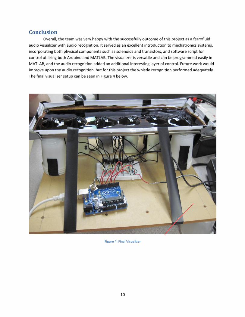
10
Conclusion Overall, the team was very happy with the successfully outcome of this project as a ferrofluid
audio visualizer with audio recognition. It served as an excellent introduction to mechatronics systems,
incorporating both physical components such as solenoids and transistors, and software script for
control utilizing both Arduino and MATLAB. The visualizer is versatile and can be programmed easily in
MATLAB, and the audio recognition added an additional interesting layer of control. Future work would
improve upon the audio recognition, but for this project the whistle recognition performed adequately.
The final visualizer setup can be seen in Figure 4 below.
Figure 4: Final Visualizer

11
Appendix A: MATLAB Code
PWM Beat Generator % ME 445 Project % Continuous spectral frequency
clear clc
% establishing Arduino connection alpha = arduino('COM6');
% setting pins to output alpha.pinMode(3,'output') alpha.pinMode(5,'output') alpha.pinMode(6,'output') alpha.pinMode(9,'output') alpha.pinMode(10,'output') alpha.pinMode(11,'output') alpha.pinMode(12,'input')
Pin = [3 5 6 9 10 11];
Ascii = 0;
while Ascii == 0; for PWM = 50:255 for k = 1:6 alpha.analogWrite(Pin(k),PWM) end end
for PWM = fliplr(50:255) for k = 1:6 alpha.analogWrite(Pin(k),PWM) end end
% killswitch value = alpha.digitalRead(12); if value == 0 Ascii = 1; else Ascii = 0; end end

12
Transverse Wave Generator % ME 445 Project % Continuous spectral frequency
clear clc
% establishing Arduino connection alpha = arduino('COM6');
% setting pins to output alpha.pinMode(3,'output') alpha.pinMode(5,'output') alpha.pinMode(6,'output') alpha.pinMode(9,'output') alpha.pinMode(10,'output') alpha.pinMode(11,'output') alpha.pinMode(12,'input')
Pin = [3 5 6 9 10 11];
Ascii = 0;
while Ascii == 0; for k = 1:6 alpha.analogWrite(Pin(k),200) pause(.1); alpha.analogWrite(Pin(k),0)
end
for k = [5 4 3 2] alpha.analogWrite(Pin(k),200) pause(.1); alpha.analogWrite(Pin(k),0)
end
% killswitch value = alpha.digitalRead(12); if value == 0 Ascii = 1; else Ascii = 0; end end

13
Random Generator % ME 445 Project % Continuous spectral frequency
clear clc
% establishing Arduino connection alpha = arduino('COM6');
% setting pins to output alpha.pinMode(3,'output') alpha.pinMode(5,'output') alpha.pinMode(6,'output') alpha.pinMode(9,'output') alpha.pinMode(10,'output') alpha.pinMode(11,'output') alpha.pinMode(12,'input')
Pin = [3 5 6 9 10 11];
Ascii = 0; n = 1;
while Ascii == 0;
k = ceil(6*rand(n)); alpha.analogWrite(Pin(k),255) pause(.1); alpha.analogWrite(Pin(k),0)
% killswitch value = alpha.digitalRead(12); if value == 0 Ascii = 1; else Ascii = 0; end end

14
Whistle Audio Recognition % ME 445 Project % Continuous spectral frequency
clear clc
% establishing Arduino connection alpha = arduino('COM6');
% setting pins to output alpha.pinMode(3,'output') alpha.pinMode(5,'output') alpha.pinMode(6,'output') alpha.pinMode(9,'output') alpha.pinMode(10,'output') alpha.pinMode(11,'output') alpha.pinMode(12,'input')
Pin = [3 5 6 9 10 11];
% user parameters duration = .1; % How many seconds of acquisition per plot refresh Fs = 5000; %Hz nBits = 16; nChannels = 1; deviceID = 2;
%Sound = analoginput('winsound'); % calls sound card %addchannel(Sound, 1); % opens channel to use %set (Sound, 'SampleRate', Fs); % sample rate (Hz) %set(Sound, 'SamplesPerTrigger', duration*Fs); % total samples per run sound = audiorecorder(Fs,nBits,nChannels,deviceID); % calls sound card & sets
up audio object
% filter settings wn = [0.125]; % cuttoff frequency 1 ---> fs/2 [b,a] = butter(2,wn,'high'); % high-pass filter
% Loop to get data and display it % this "try" helps the program end % properly when "ctr+c" is hit
figure(1010) count = 0;
Ascii = 0;
while Ascii == 0 % count how many times the while was executed
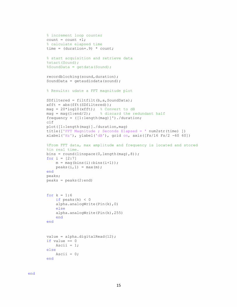
15
% increment loop counter count = count +1; % calculate elapsed time time = (duration+.9) * count;
% start acquisition and retrieve data %start(Sound); %SoundData = getdata(Sound);
recordblocking(sound,duration); SoundData = getaudiodata(sound);
% Results: udate a FFT magnitude plot
SDfiltered = filtfilt(b,a,SoundData); xfft = abs(fft(SDfiltered)); mag = 20*log10(xfft); % Convert to dB mag = mag(1:end/2); % discard the redundant half frequency = ([1:length(mag)]')./duration; clf plot([1:length(mag)]./duration,mag) title(['FFT Magnitude ; Seconds Elapsed = ' num2str(time) ]) xlabel('Hz'), ylabel('dB'), grid on, axis([Fs/16 Fs/2 -60 60])
%From FFT data, max amplitude and frequency is located and stored %in real time. bins = round(linspace(0,length(mag),8)); for i = [2:7] m = mag(bins(i):bins(i+1)); peaks(i,1) = max(m); end peaks; peaks = peaks(2:end)
for k = 1:6 if peaks(k) < 0 alpha.analogWrite(Pin(k),0) else alpha.analogWrite(Pin(k),255) end end
value = alpha.digitalRead(12); if value == 0 Ascii = 1; else Ascii = 0; end
end

16
Appendix B: Datasheets


TIP120/121/122TIP125/126/127
COMPLEMENTARY SILICON POWER DARLINGTON TRANSISTORS
STMicroelectronics PREFERREDSALESTYPES
DESCRIPTION The TIP120, TIP121 and TIP122 are siliconEpitaxial-Base NPN power transistors inmonolithic Darlington configuration mounted inJedec TO-220 plastic package. They are intentedfor use in power linear and switching applications.The complementary PNP types are TIP125,TIP126 and TIP127, respectively.
INTERNAL SCHEMATIC DIAGRAM
March 2000
ABSOLUTE MAXIMUM RATINGS
Symbol Parameter Value Unit
NPN TIP120 TIP121 TIP122
PNP TIP125 TIP126 TIP127
VCBO Collector-Base Voltage (IE = 0) 60 80 100 V
VCEO Collector-Emitter Voltage (IB = 0) 60 80 100 V
VEBO Emitter-Base Voltage (IC = 0) 5 V
IC Collector Current 5 A
ICM Collector Peak Current 8 A
IB Base Current 0.1 A
Ptot Total Dissipation at Tcase ≤ 25 oC Tamb ≤ 25 oC
652
WW
Tstg Storage Temperature -65 to 150 oC
Tj Max. Operating Junction Temperature 150 oC* For PNP types voltage and current values are negative.
12
3
TO-220
R1 Typ. = 5 KΩ R2 Typ. = 150 Ω
1/4

THERMAL DATA
Rthj-case
Rthj-amb
Thermal Resistance Junction-case MaxThermal Resistance Junction-ambient Max
1.9262.5
oC/WoC/W
ELECTRICAL CHARACTERISTICS (Tcase = 25 oC unless otherwise specified)
Symbol Parameter Test Conditions Min. Typ. Max. Unit
ICEO Collector Cut-offCurrent (IB = 0)
for TIP120/125 VCE = 30 Vfor TIP121/126 VCE = 40 Vfor TIP122/127 VCE = 50 V
0.50.50.5
mAmAmA
ICBO Collector Cut-offCurrent (IB = 0)
for TIP120/125 VCB = 60 Vfor TIP121/126 VCB = 80 Vfor TIP122/127 VCB = 100 V
0.20.20.2
mAmAmA
IEBO Emitter Cut-off Current(IC = 0)
VEB = 5 V 2 mA
VCEO(sus)* Collector-EmitterSustaining Voltage(IB = 0)
IC = 30 mAfor TIP120/125for TIP121/126for TIP122/127
6080
100
VVV
VCE(sat)* Collector-EmitterSaturation Voltage
IC = 3 A IB = 12 mAIC = 5 A IB = 20 mA
24
VV
VBE(on)* Base-Emitter Voltage IC = 3 A VCE = 3 V 2.5 V
hFE* DC Current Gain IC = 0.5 A VCE = 3 VIC = 3 A VCE = 3 V
10001000
∗ Pulsed: Pulse duration = 300 µs, duty cycle < 2 %For PNP types voltage and current values are negative.
TIP120/TIP121/TIP122/TIP125/TIP126/TIP127
2/4
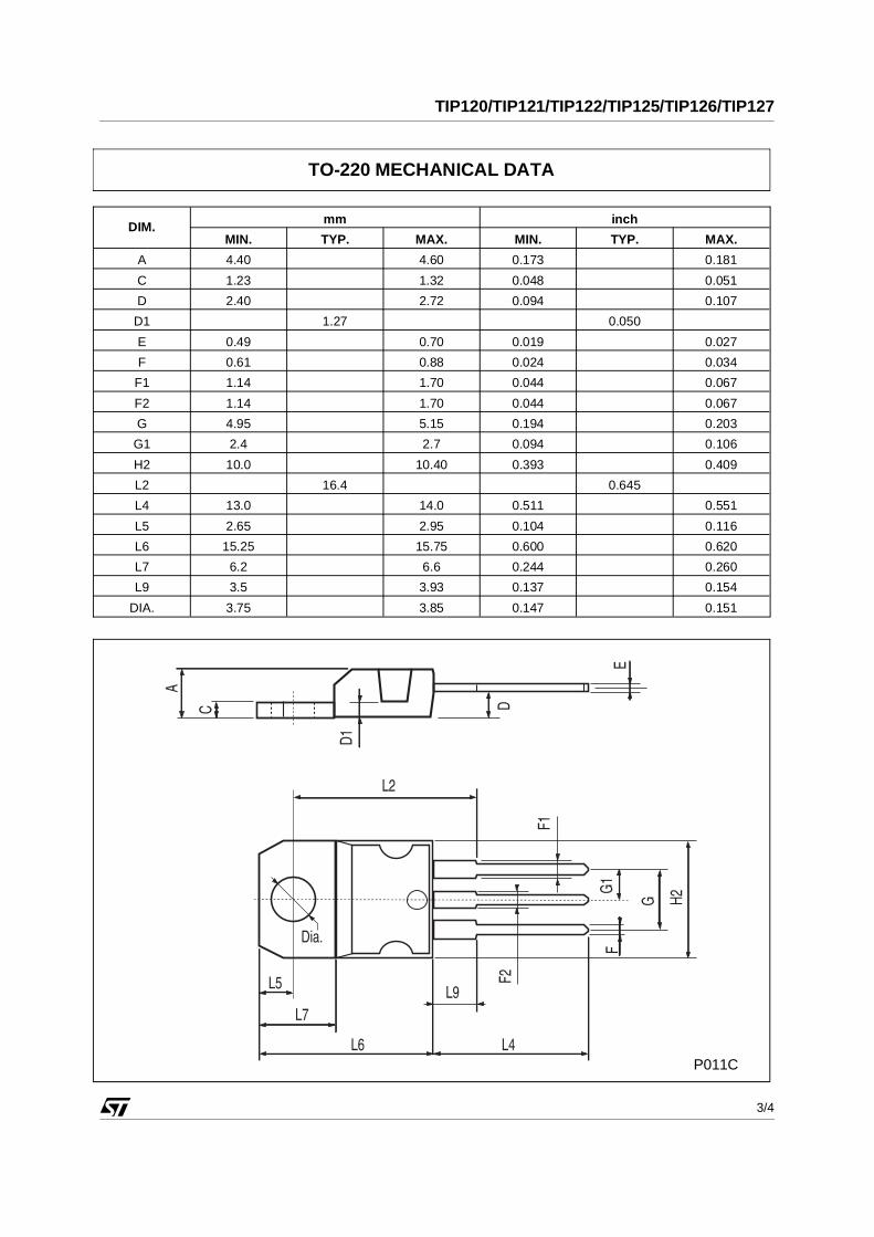
DIM.mm inch
MIN. TYP. MAX. MIN. TYP. MAX.
A 4.40 4.60 0.173 0.181
C 1.23 1.32 0.048 0.051
D 2.40 2.72 0.094 0.107
D1 1.27 0.050
E 0.49 0.70 0.019 0.027
F 0.61 0.88 0.024 0.034
F1 1.14 1.70 0.044 0.067
F2 1.14 1.70 0.044 0.067
G 4.95 5.15 0.194 0.203
G1 2.4 2.7 0.094 0.106
H2 10.0 10.40 0.393 0.409
L2 16.4 0.645
L4 13.0 14.0 0.511 0.551
L5 2.65 2.95 0.104 0.116
L6 15.25 15.75 0.600 0.620
L7 6.2 6.6 0.244 0.260
L9 3.5 3.93 0.137 0.154
DIA. 3.75 3.85 0.147 0.151
P011C
TO-220 MECHANICAL DATA
TIP120/TIP121/TIP122/TIP125/TIP126/TIP127
3/4

Information furnished is believed to be accurate and reliable. However, STMicroelectronics assumes no responsibility for the consequencesof use of such information nor for any infringement of patents or other rights of third parties which may result from its use. No license isgranted by implication or otherwise under any patent or patent rights of STMicroelectronics. Specification mentioned in this publication aresubject to change without notice. This publication supersedes and replaces all information previously supplied. STMicroelectronics productsare not authorized for use as critical components in life support devices or systems without express written approval of STMicroelectronics.
The ST logo is a trademark of STMicroelectronics
© 2000 STMicroelectronics – Printed in Italy – All Rights ReservedSTMicroelectronics GROUP OF COMPANIES
Australia - Brazil - China - Finland - France - Germany - Hong Kong - India - Italy - Japan - Malaysia - Malta - Morocco - Singapore - Spain - Sweden - Switzerland - United Kingdom - U.S.A.
http://www.st.com
TIP120/TIP121/TIP122/TIP125/TIP126/TIP127
4/4

ME 445 Robotic Segway
“Dexterous”
David Patzer and Dan Karrasch
May 2nd
2013
Final Report
2
Contents Introduction ................................................................................................................................................... 3
Construction of Robot ................................................................................................................................... 3
Gathering Parts.......................................................................................................................................... 3
Modeling the System .................................................................................................................................... 4
Free body Diagram: .................................................................................................................................. 4
State Space Model ..................................................................................................................................... 6
Calculating the Moment of Inertia ................................................................................................................ 7
Finding the Natural Frequency and Damping Coefficient ........................................................................ 7
Controller ...................................................................................................................................................... 9
Relating Voltage to Torque ..................................................................................................................... 10
Technical issues .......................................................................................................................................... 12
Conclusions and Results ............................................................................................................................. 13
Appendix ..................................................................................................................................................... 14
A. Sources ............................................................................................................................................... 14
B. Datasheets........................................................................................................................................... 14
C. Matlab Code for Solving State Space Model ..................................................................................... 15
D. Arduino Code for Gathering Moment of Inertia Data ........................................................................ 18
E. Arduino Code for Balancing the Robot .............................................................................................. 20

3
Introduction
The purpose of this project is to create a two wheeled self-balancing robot. The inspiration for this was a
Segway personal transportation device and the ease of which it balances on two wheels with a person
riding it. The robot will require a robust control system that can quickly react to changes to in the robots
position and angle. The system is naturally unstable and will require proper analysis to create a nearly
perfect control system. The project can be broken down into three simple steps, the construction of the
robot, the modeling of the system using Arduino and Matlab, and the construction of the controller.
Construction of Robot
Gathering Parts Table one contains a listing of all the parts used to create the balancing robot. Quantity, vendor, and price
are included as well. The total cost of parts excluding parts found in the lab comes to $172.23.
Part Quantity Vendor Price Arduino Uno 1 Amazon.com $20
Pololu Motor: 34:1 Metal Gearmotor
25Dx52L mm with 48 CPR Encoder
2 Pololu Robotics & Electronics $70
Pololu Dual MC33926 Motor Driver
Shield
1 Pololu Robotics & Electronics $30
MPU6050 Accelerometer and Gyroscope 1 Amazon.com $17
7474 D Flip Flop 1 DigiKey Electronics $1.73
Pololu Wheel Set 90x10mm Black 1 Pololu Robotics & Electronics $10
Pololu Universal Aluminum Mounting
Hub for 5mm Shaft Pair
1 Pololu Robotics & Electronics $7.50
9.6v Battery 1 Amazon.com $16
Miscellaneous pieces of wood 4 - -
Motor Mounts 2 - -
Mini Bread Board 1 - -
Screws 14 - -
Total Cost $172.23
Table 1
Headers and terminal blocks were soldered onto the Pololu motor shield. It then fits perfectly in the
Arduino Uno’s pins. The circuit was then wired according to the schematic in figure one.

4
Figure 1
Modeling the System
Free body Diagram: A self-balancing robot can be modeled as an inverted pendulum swinging freely on top of a cart. The
University of Michigan has an excellent controls tutorial for an inverted pendulum which we relied
heavily on to do our analysis of our system. All equations were hand derived from scratch to verify their
accuracy. Figure two shows a diagram of the free body diagram from the University of Michigan’s
tutorial.

5
Where F is the force on the cart from the motors, m is the mass of the pendulum, M is the mass of the
cart, l is the length from the rotational axis to the center of mass of the pendulum, I is the moment of
inertia of the pendulum, b is the coefficient of friction for the cart, and x is the cart position coordinate.
The equations of motion were then derived by summing the forces and moments. The two equations of
motion are as follows:
By linearizing these equations they can be placed into a state space model to be used in Matlab.
Assuming small angles, the following assumptions can be made:
Figure 2

State Space Model The linearized equations of motion can be written in standard matrix form as seen in figure three from the
University of Michigan’s Tutorial.
A Matlab m file was created to solve the state space model using the “ss” command. The m file is
included in appendix A. Before solving the system, some of the system parameters needed to be found.
The first system parameters to be found were the two masses. The robot was deconstructed so that the
mass of the pendulum and the mass of the cart could be weighted. The mass of the pendulum (m) part of
the robot came to .562 kg and the mass of the cart (M) came to .498 kg. After putting the robot back
together it was balanced on a rod to find its center of gravity which came out to .045m from the axis of
rotation. The only missing system parameter is the moment of inertia which requires some additional
work to obtain.
Figure 3

Calculating the Moment of Inertia To find the moment of inertia of the robot we will be using the equation:
All the variables in the equation are known except for the angular frequency and damping coefficient. The
angular frequency can be derived from the natural frequency once it is calculated by using the equation:
Finding the Natural Frequency and Damping Coefficient To find the natural frequency the robot was flipped upside down and used as a regular pendulum. It was
attached to two boards which were places on either side of a gap between two tables. A picture of the
setup is shown in figure four below.
Figure 4
This allowed the robot to swing back and forth freely like a pendulum. An Arduino sketch was created to
output encoder position in degrees and time in milliseconds to the serial port which is included in
appendix D. The robot was dropped from parallel to the floor and was allowed to swing freely until
coming to a complete stop. This was done five times and the data was graphed in excel, which is shown in
figure five.
8
Figure 5
Two data points were then taken from each data set at the max of the first two oscillations. The time at
which the max occurred and its amplitude were recorded in table two, below. The natural frequency is
calculated by dividing the number of cycles (in this case 1) by the amount of time it takes to complete
those cycles. We calculated the natural frequency for each data set and then averaged them together to
obtain the natural frequency of our system. By using the angular frequency equation above we were able
to convert the natural frequency to an angular frequency for use in the moment of inertia equation.
The damping coefficient of the system can be found by analyzing the decrease in amplitude of one max to
another using the equation:
Where Af is the amplitude of the second max, Ai is the amplitude of the first max, b is the damping
coefficient, t is the amount of time between maxes, and m is the mass of the pendulum. The damping
coefficient was calculated for each data set using the amplitudes recorded in table two. The five
coefficients were averaged together to obtain the damping coefficient of the system.

9
Table 2
Controller
The controller for the robot uses proportional control and derivative control in the form of the following
equation.
Where x is linear position determined from the encoders, x’ is the linear velocity derived from the linear
position, θ is Euler angle β from the gyroscope and accelerometer, and θ’ is the angular rotation from the
gyroscope.
Matlab was used to calculate the proportional and derivative gains, a, b, c, and d. The code can be found
in appendix C. It uses the state space model from above to calculate the coefficients using the ss function.
The coefficients are output from the variable “K”. The Matlab code also produces a plot that shows what
a step response of the system will look like. This plot can be seen in figure six.
Time (s) Position (Degrees) Natural Frequency (Hz) Damping Coefficient
Run 1 1.018 359
2.271 305
Run 2 1.486 358
2.715 304
Run 3 0.686 368
1.913 315
Run 4 0.687 364
1.857 306
Run 5 0.67 363
1.842 307
Average 0.82693867 0.337597326
0.367609122
0.853242321 0.354266895
0.854700855
0.798084597 0.322377982
0.81366965 0.329670797
0.814995925 0.314061833
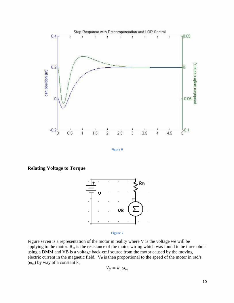
10
Figure 6
Relating Voltage to Torque
Figure 7
Figure seven is a representation of the motor in reality where V is the voltage we will be
applying to the motor. Rm is the resistance of the motor wiring which was found to be three ohms
using a DMM and VB is a voltage back-emf source from the motor caused by the moving
electric current in the magnetic field. VB is then proportional to the speed of the motor in rad/s
(ωm) by way of a constant kv

11
The current flowing through the motor can be found using ohms law and is equivalent to the
following equation.
On the mechanical side of the analysis, the torque from the motor is proportional to the amount
of current flowing through the motor by way of a constant kt.
The torque equation can then be substituted into the current equation to obtain:
Then substitute in the VB equation to get:
Then solve for V to get the voltage equation to apply to the motor.
Now because our controller equation is a force, not a torque, the torque has to be rewritten as:
Where F is a force in newtons and r is the radius of the wheels in meters. The final equation
looks like:
Where:
The two constant kt and kv will be equal assuming a perfectly efficient motor. Kv can be found
by graphing rotational velocity of the motor and voltage applied to the motor to see if it is linear.
The slope of the linear equation will then be equal to kt and kv. We applied a known voltage to
our motor and had the serial port print out rotational velocity using the encoders. We then
graphed this data in excel and found that it was indeed linear. A linear trend line was applied to
the data which a slope of .7163 which is equivalent to kv and kt. .
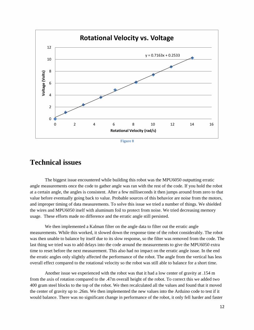
12
Figure 8
Technical issues
The biggest issue encountered while building this robot was the MPU6050 outputting erratic
angle measurements once the code to gather angle was ran with the rest of the code. If you hold the robot
at a certain angle, the angles is consistent. After a few milliseconds it then jumps around from zero to that
value before eventually going back to value. Probable sources of this behavior are noise from the motors,
and improper timing of data measurements. To solve this issue we tried a number of things. We shielded
the wires and MPU6050 itself with aluminum foil to protect from noise. We tried decreasing memory
usage. These efforts made no difference and the erratic angle still persisted.
We then implemented a Kalman filter on the angle data to filter out the erratic angle
measurements. While this worked, it slowed down the response time of the robot considerably. The robot
was then unable to balance by itself due to its slow response, so the filter was removed from the code. The
last thing we tried was to add delays into the code around the measurements to give the MPU6050 extra
time to reset before the next measurement. This also had no impact on the erratic angle issue. In the end
the erratic angles only slightly affected the performance of the robot. The angle from the vertical has less
overall effect compared to the rotational velocity so the robot was still able to balance for a short time.
Another issue we experienced with the robot was that it had a low center of gravity at .154 m
from the axis of rotation compared to the .47m overall height of the robot. To correct this we added two
400 gram steel blocks to the top of the robot. We then recalculated all the values and found that it moved
the center of gravity up to .26m. We then implemented the new values into the Arduino code to test if it
would balance. There was no significant change in performance of the robot, it only fell harder and faster
y = 0.7163x + 0.2533
0
2
4
6
8
10
12
0 2 4 6 8 10 12 14 16
Vo
ltag
e (
Vo
lts)
Rotational Velocity (rad/s)
Rotational Velocity vs. Voltage

13
resulting in longer repair times between tests. The weights were removed and old values put back into the
Arduino code. If the erratic angle data were able to be removed, the higher center of gravity would be
more desirable. For the sake of our project, it was not practical.
Conclusions and Results
In the end, the robot was able to balance for a short amount of time at small angles. Mapping of the power
to the motors had to be done by hand to scale the power coming from the controller. This was done with
the Arduino map function. Solving the erratic angle issue along with increasing the height of the center
of gravity would result in a more stable robot that could balance for longer periods of time.
A short video of the robot in action can be found here: http://youtu.be/ffySoPVitwo
Overall we learned how to create a proportional and derivative controller using a state space model of an
inverted pendulum using a combination of Matlab and Arduino code. We used Arduino libraries and
controls tutorials that were available to help with modeling the system and coding the Arduino. With a
relatively expensive total cost and in-depth coding, this is not a simple project. Many hours were spent
debugging and perfecting the code, however some technical issues persist.

Appendix
A. Sources
University of Michigan control tutorial for an inverted pendulum:
Equations of Motion
State Space Model
http://ctms.engin.umich.edu/CTMS/index.php?example=InvertedPendulum§ion=SystemModeling
DC Motor Analysis:
http://electronics.stackexchange.com/questions/39387/how-are-current-and-voltage-related-to-torque-and-
speed-of-a-brushless-motor
B. Datasheets
Pololu Motor: 34:1 Metal Gearmotor 25Dx52L mm with 48 CPR Encoder:
http://www.pololu.com/catalog/product/2284
Pololu Dual MC33926 Motor Driver Shield
http://www.pololu.com/docs/0J55
MPU6050 Accelerometer and Gyroscope
http://playground.arduino.cc/Main/MPU-6050
http://invensense.com/mems/gyro/documents/PS-MPU-6000A.pdf
7474 D Flip-Flop
http://www.ti.com/lit/ds/symlink/sn74als576b.pdf

15
C. Matlab Code for Solving State Space Model
%Inverted Pendulum Model %ME 445 - H. J. Sommer %Penn State University %Daniel Karrasch %David Patzer %May 2, 2013
%References: %http://ctms.engin.umich.edu/CTMS/index.php?example=InvertedPendulum§ion=
ControlStateSpace % -From Michigan University
%------------------------------------------------------------------------ %This Matlab code uses the derived state space model of the system to %determine the gain coefficients for each variable: x, xdot, theta, %thetadot. %------------------------------------------------------------------------
clear clc
t = 0:0.01:2; %time matrix u = zeros(size(t)); %zero matrix x0 = [.1 0 0 0]; %initial push
M = .498; %mass of cart in kg m = .562 ; %mass of pendulumin kg b = 0.337597; %damping coefficient f= .8269272;%Natural Frequency (Hz)
g = 9.8; %gravity m/s^2 l = .154; %length from center of motors to center of gravity in meters
% Mass Moment of Inertia Calculation
w= f*2*pi(); %angular frequency I= (((M+m).*g*l)/w^2)+(M+m)*l^2; %mass moment of intertia of cart
p = I*(M+m)+M*m*l^2; %denominator for the A and B matrices
%---State Space Model--- %matrices are result of state space derivation A = [0 1 0 0; 0 -(I+m*l^2)*b/p (m^2*g*l^2)/p 0; 0 0 0 1; 0 -(m*l*b)/p m*g*l*(M+m)/p 0] B = [ 0; (I+m*l^2)/p; 0;

16
m*l/p]; C = [1 0 0 0; 0 0 1 0]; D = [0; 0];
states = 'x' 'x_dot' 'phi' 'phi_dot'; inputs = 'u'; %input force outputs = 'x'; 'phi';
%Solve the state space model sys_ss =
ss(A,B,C,D,'statename',states,'inputname',inputs,'outputname',outputs);
poles = eig(A); %one right half plane pole means system is unstable
%---Controllability--- co = ctrb(sys_ss); controllability = rank(co); %result of controllability=4 means that all state space variables can be %solved and the system is controllable.
%---Weighting the variables--- %Q and R give weighting to the various state space variables. Q = C'*C; Q(1,1) = 5000; Q(3,3) = 100; %Making these values larger adds more value to these state
variables. R = 1;
%---Linear Quadratic Regulation--- % output the coefficients K = lqr(A,B,Q,R) %These k values correlate to a,b,c, and d coefficient gains in Arduino code
%New state space matrices with weights Ac = [(A-B*K)]; Bc = [B]; Cc = [C]; Dc = [D];
states = 'x' 'x_dot' 'phi' 'phi_dot'; inputs = 'r'; outputs = 'x'; 'phi';
Cn = [1 0 0 0]; %Focuses on an initial displacement of cart
%---Run Simulation--- sys_ss = ss(A,B,Cn,0); Nbar = rscale(sys_ss,K) sys_cl =
ss(Ac,Bc*Nbar,Cc,Dc,'statename',states,'inputname',inputs,'outputname',output
s);
t = 0:0.01:5;

17
r =0.2*ones(size(t)); [y,t,x]=lsim(sys_cl,r,t); [AX,H1,H2] = plotyy(t,y(:,1),t,y(:,2),'plot'); set(get(AX(1),'Ylabel'),'String','cart position (m)') set(get(AX(2),'Ylabel'),'String','pendulum angle (radians)') title('Step Response with Precompensation and LQR Control')
function[Nbar] = rscale(a,b,c,d,k)
% Given the single-input linear system: % . % x = Ax + Bu % y = Cx + Du % and the feedback matrix K, % % the function rscale(sys,K) or rscale(A,B,C,D,K) % finds the scale factor N which will % eliminate the steady-state error to a step reference % for a continuous-time, single-input system % with full-state feedback using the schematic below: % % /---------\ % R + u | . | % ---> N --->() ----> | X=Ax+Bu |--> y = Cx ---> y % -| \---------/ % | | % |<---- K <----| % % 8/21/96 Yanjie Sun of the University of Michigan % under the supervision of Prof. D. Tilbury % 6/12/98 John Yook, Dawn Tilbury revised error(nargchk(2,5,nargin));
% --- Determine which syntax is being used --- nargin1 = nargin;
if (nargin==2), % System form
[A,B,C,D] = ssdata(a); K=b;
elseif (nargin==5), % A,B,C,D matrices A=a; A = a; B = b; C = c; D = d; K = k; else error('Input must be of the form (sys,K) or (A,B,C,D,K)') end;
% compute Nbar s = size(A,1); s = size(A,1); Z = [zeros([1,s]) 1]; N = inv([A,B;C,D])*Z'; Nx = N(1:s); Nu = N(1+s); Nbar = Nu + K*Nx;

18
D. Arduino Code for Gathering Moment of Inertia Data
//****************************************************************//
//Arduino Code for Gathering Moment of Inertia Data for a Pendulum //
//****************************************************************//
//This variable changes value everytime the encoder sees a positive or negative edge.
volatile float encoder_position;
//A TTL 7474 flip flop was used to obtain direction of the motor.
volatile float flip_flop=11;
//this is a 1 or 0 depending on whether the motor is running clockwise or //counterclockwise.
volatile int flip_flop_value;
// Set the beginning time value to 0
int time=0;
void setup()
// Declare pin mode for flip flop chip
pinMode(flip_flop,INPUT);
//Start the interrupt on pin 3
attachInterrupt(1,increment, CHANGE);
//Initalize serial communication
Serial.begin(115200);
void loop()
//Record time
time=millis();
//Print time value to the serial port.
Serial.print(time);
// Print a space and encoder position
Serial.print("\t");
Serial.println(encoder_position);
//End serial after 10 seconds
if (time>=10000)
Serial.end();

19
//========================================================//
// //
// Functions //
// //
//========================================================//
void increment()
//This function is called once digital pin 2 (also called interrupt 0) changes state.
//It must add or subtract from motor_position that holds the number of degrees the motor has
turned.
//Reads a 1 or 0 out of the flip flop
flip_flop_value=digitalRead(flip_flop);
//If A leads B, there is an output of 1
// subtract 1 from encoder position if flip-flop=1
if ((flip_flop_value==1))
encoder_position--;
//Add 1 to encoder position if flip-flop=0
else
encoder_position++;

20
E. Arduino Code for Balancing the Robot
/*
Inverted Pendulum Project
ME 445 - H J Sommer
Daniel Karrasch
David Patzer
May 2, 2013
*/
//Include Libraries
#include "Wire.h"
#include "Math.h"
#include "I2Cdev.h"
#include "MPU6050_6Axis_MotionApps20.h"
#include "DualMC33926MotorShield.h"
DualMC33926MotorShield md;
MPU6050 mpu;
MPU6050 accelgyro;
#define LED_PIN 13 // (Arduino is 13, Teensy is 11, Teensy++ is 6)
bool blinkState = false;
bool dmpReady = false; // set true if DMP init was successful
uint8_t mpuIntStatus; // holds actual interrupt status byte from MPU
uint8_t devStatus; // return status after each device operation (0 = success, !0 = error)
uint16_t packetSize; // expected DMP packet size (default is 42 bytes)
uint16_t fifoCount; // count of all bytes currently in FIFO
uint8_t fifoBuffer[64]; // FIFO storage buffer
Quaternion q; // [w, x, y, z] quaternion container
float euler[3]; // [psi, theta, phi] Euler angle container
volatile bool mpuInterrupt = false; // indicates whether MPU interrupt pin has gone high
void dmpDataReady()
mpuInterrupt = true;
// =======Setup Global Variables ========//
//Variables for storing the raw accelerometer values, ax for x values, ay for y value, az for z values.
int16_t ax, ay, az;
//Variales for storing the raw gyroscope values, gx for x values, gy for y values, gz for z values.
int16_t gx, gy, gz;
//This variable changes value everytime the encoder sees a positive or negative edge.
volatile float encoder_position;
//Variable for holding how far away the robot has moved from its starting point.
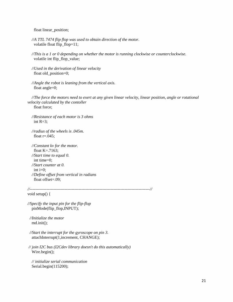
21
float linear_position;
//A TTL 7474 flip flop was used to obtain direction of the motor.
volatile float flip_flop=11;
//This is a 1 or 0 depending on whether the motor is running clockwise or counterclockwise.
volatile int flip_flop_value;
//Used in the derivation of linear velocity
float old_position=0;
//Angle the robot is leaning from the vertical axis.
float angle=0;
//The force the motors need to exert at any given linear velocity, linear position, angle or rotational
velocity calculated by the contoller
float force;
//Resistance of each motor is 3 ohms
int R=3;
//radius of the wheels is .045m.
float r=.045;
//Constant kv for the motor.
float K=.7163;
//Start time to equal 0.
int time=0;
//Start counter at 0.
int i=0;
//Define offset from vertical in radians
float offset=.09;
//--------------------------------------------------------------------------------------//
void setup()
//Specify the input pin for the flip-flop
pinMode(flip_flop,INPUT);
//Initialize the motor
md.init();
//Start the interrupt for the gyroscope on pin 3.
attachInterrupt(1,increment, CHANGE);
// join I2C bus (I2Cdev library doesn't do this automatically)
Wire.begin();
// initialize serial communication
Serial.begin(115200);

22
// initialize devices
mpu.initialize();
// load and configure the DMP
devStatus = mpu.dmpInitialize();
// make sure it worked (returns 0 if so)
if (devStatus == 0)
// turn on the DMP
mpu.setDMPEnabled(true);
// enable Arduino interrupt detection
attachInterrupt(0, dmpDataReady, RISING);
mpuIntStatus = mpu.getIntStatus();
// set our DMP Ready flag so the main loop() function knows it's okay to use it
dmpReady = true;
// get expected DMP packet size for later comparison
packetSize = mpu.dmpGetFIFOPacketSize();
else
// ERROR!
// 1 = initial memory load failed
// 2 = DMP configuration updates failed
// (if it's going to break, usually the code will be 1)
Serial.print(F("DMP Initialization failed (code "));
Serial.print(devStatus);
Serial.println(F(")"));
// configure LED for output
pinMode(LED_PIN, OUTPUT);
//----------------------------------------------------------------------------//
void loop()
//Count each loop
i=i+1;
/* //Uncomment this section to view time and counts
Serial.print(time);
Serial.print("\t");
Serial.print(i);
Serial.println("\t");
*/
//Defines new position
float new_position;
//Defines previous time
int time_old=time;

23
time=millis();
//Defines current time
int time_new=time;
new_position=linear_position;
//Linear Velocity Calculation using finite differencing
float linear_velocity= 1000*(new_position-old_position)/(time_new-time_old);
//Rotational velocity of the wheels are calculated - Needed for later
float motor_rotational_velocity= linear_velocity/r;
//Defines old position
old_position=linear_position;
//~~~~~~~~~~Display Euler angles in degrees~~~~~~~~~~~~~~~~~~~~~~~//
// wait for MPU interrupt or extra packet(s) available
while (!mpuInterrupt && fifoCount < packetSize)
// reset interrupt flag and get INT_STATUS byte
mpuInterrupt = false;
mpuIntStatus = mpu.getIntStatus();
// get current FIFO count
fifoCount = mpu.getFIFOCount();
// check for overflow (this should never happen unless our code is too inefficient)
if ((mpuIntStatus & 0x10) || fifoCount == 1024)
// reset so we can continue cleanly
mpu.resetFIFO();
// otherwise, check for DMP data ready interrupt (this should happen frequently)
else if (mpuIntStatus & 0x02)
// wait for correct available data length, should be a VERY short wait
while (fifoCount < packetSize) fifoCount = mpu.getFIFOCount();
// read a packet from FIFO
mpu.getFIFOBytes(fifoBuffer, packetSize);
// track FIFO count here in case there is > 1 packet available
// (this lets us immediately read more without waiting for an interrupt)
fifoCount -= packetSize;
// Get Quaternion and euler angle values from the gyroscope/accelerometer
mpu.dmpGetEuler(euler, &q);

24
// Put Euler angle Beta in the angle variable while offsetting it to zero
float angle= (euler[1]+offset);
//Multiply by 1000 for better resolution. Will be divided by 1000 later
angle=angle*1000;
//Serial.println(angle); //Uncomment to view angle*1000
//~~~~~~~~~~~~~~~~~~~~~~~~Gyroscope ~~~~~~~~~~~~~~~~~~~~~~~~~~~~~~~~~//
// Get the raw gyroscope values from the gyroscope
mpu.getRotation(&gx, &gy, &gz);
//~~~~~~~~~~~~~~~Function Calls~~~~~~~~~~~~~~~~~~~~~~~~~~~~~~~~~~~//
// Calling the controller function with linear position,linear velocity, angle, and rotational veloctiy (gy)
as inputs
controller(linear_position, linear_velocity,angle, gy);
// Calling the Motor_power function with force (from the controller) and motor_rotational_velocity as
inputs.
Motor_power(force, motor_rotational_velocity);
/* //Uncomment this section to view the 4 state variables before the gain coefficients
Serial.print(linear_position);
Serial.print("\t");
Serial.print(linear_velocity);
Serial.print("\t");
Serial.println(angle);
Serial.print("\t");
Serial.print(gy-40);
Serial.print("\t");
*/
//=============================================================//
// //
// Functions //
// //
//=============================================================//
void increment()
//This function is called once digital pin 3 (also called interrupt 1) changes state.
//It adds or subtracts from encoder_position that holds the number of degrees the motor has turned.
//Reads a 1 or 0 out of the flip flop.
flip_flop_value=digitalRead(flip_flop);
if ((flip_flop_value==1))
//If A leads B, there is an output of 1

25
encoder_position--;
//Given the direction of the motor, the encoder position decreases by 1 degree per step.
linear_position=encoder_position*2*2*PI*r/1633; //Radius of wheel is 2in; 1633*180 = 293940
else
//If B leads A, there is an output of 0
encoder_position++;
//Given the direction of the motor, the encoder position increases by 1 degree per step.
linear_position=encoder_position*2*2*PI*r/1633; //Convert to meters; (1633 steps/rev)
// The controller uses proportional and derivative control on the linear position for the robot and its
angle from the vertical.
void controller( float linear_position, float linear_velocity, float angle, float gy )
//The following values were calculated from the state space model in matlab
// Coefficient for linear position
int a=-71;
//Coefficient for linear velocity
int b=-60;
//Coefficient for angle
int c=-259;
//Coefficient for rotational velocity
int d=88;
//Serial.println(angle);
/*
The following if statements are an attempt to optimize the behavior of the robot.
The first two if statements prevent the motor from completely stopping when the
segway is at low angles relative to vertical.
The third if statement prevents the robot from moving erratically whenever the
sensor cuts out and outputs only 0.
*/
if (angle > 0 && angle < 40) //If 0<theta<40, angle =40
angle=40;
else if (angle < 0 && angle > -40) //If -40<theta<0, angle=-40
angle=-40;
//If sensor cuts out and outputs only zero, oscillate the perceived angle between 40 and -40
//This hopefully keeps it somewhat stabiized until the sensor is working again.
else if (angle == 0 || angle== -0)
if ( (i % 2) == 0)

26
angle=40;
else
angle=-40;
else //Anything outside of small thetas should be perceived as normal.
angle=angle;
angle=angle/1000; //Dividing theta by 1000 since we multiplied it by 1000 earlier.
//Gyroscope - Theta_dot values.
//There seems to be an offset of 40 deg/sec, hence the (-40)
gy=(gy-40)*PI/180; //Convert to rad/sec
gy=constrain(gy, -15, 15); //Constrain theta_dot to ignore erratic behavior and/or noise.
// Calculates the amount of force the motors need to
force=(a*linear_position)+(b*linear_velocity)+(c*angle)+(d*gy);
/* //Uncomment this section to analyze all values that contribute to the "force"
Serial.print(force);
Serial.print("\t");
Serial.print(a*linear_position);
Serial.print("\t");
Serial.print(b*linear_velocity);
Serial.print("\t");
Serial.print(c*angle);
Serial.print("\t");
Serial.print(d*gy);
Serial.println("\t");
*/
void Motor_power(float force, float motor_rotational_velocity)
float power=((force*r*R)/(K))+(K*motor_rotational_velocity);
power=map(power,-100,100,-400,400);
// Serial.println(power);
md.setM1Speed(power/2);
md.setM2Speed((-power*.95)/2); //Motor two seems to be stronger, so we scaled the input power.

This project aims to develop a
microcontroller that maximizes power
output from a solar panel. A circuit that
throttles current was built using pulse
width modulation and a Darlington
transistor. An algorithm based on
maximum power point tracking was
developed to maximize the power
output. A charge controller for a battery
is the logical next step for this project.
Solar Power
Optimization ME445 Final Project
Andrew Kreider & Ray Polcino

1
Table of Contents 1. Solar Panel Considerations ...................................................................................................... 2
2. Vary Current using PWM ........................................................................................................ 3
3. Stabilize Measurements ........................................................................................................... 4
4. AD623 Implementation ........................................................................................................... 6
5. LCD Readout ........................................................................................................................... 6
6. Maximum Power Point Tracking ............................................................................................ 7
7. MPPT Test Results .................................................................................................................. 7
8. Future Work: Charge Controller .............................................................................................. 8
Appendices ...................................................................................................................................... 9
Appendix I: System Schematic ................................................................................................... 9
Appendix II: Battery Charger Considerations .......................................................................... 10
Appendix III: Battery Charger considerations .......................................................................... 11
Appendix IV: AD623AN Instrumentation Amplifier ............................................................... 12
Appendix V: Voltage Regulator ............................................................................................... 13
Appendix VI: Arduino code to use moving average ................................................................ 14
Appendix VII: Maximum Power Point Tracking (MPPT) function ......................................... 16

2
1. Solar Panel Considerations This project aims to design and build some advanced solar panel optimization circuitry. At the
time of this report, the energy industry is frantically developing many new technologies
simultaneously. Solar power shows promise because it is readily available in most regions of the
world and is expected to not be depleted. However, solar power is cyclic, unpredictable, and
does not supply energy perfectly in accordance with demand.
To address the unpredictability of
solar irradiance, a maximum power
point tracking (MPPT) code has
been developed. As seen in Figure
1, the current and voltage outputs of
a solar panel are inversely
proportional. When more current is
drawn, the voltage drops off. In the
indoor case in Figure 1 the
maximum power occurs at the
circled point. Ideally the solar panel
operates at this point for maximum
power.
Figure 2 shows the experimental
setup used to determine the data in
Figures 1 and 3. Later, the current
and voltage will be traded off using
a PWM output from an Arduino and
a TIP122 BJT. The analog setup
shown in Figure 2 gives a smoother,
closer-to-theoretical curve than the
PWM/BJT setup, which is shown in
Figure X.
Figure 3 shows that the entire curve
shifts with changing amounts of
irradiance. The black points are
measured and the gray points
simulate 15% less irradiance.
Suppose a solar panel is happily
receiving black-line irradiance and
operating at the maximum point circled in red in Figure 3. Now suppose that the irradiation
0
50
100
150
200
250
300
350
0 2 4 6 8
Cu
rren
t (m
A)
Voltage (V)
Current vs. Voltage (outdoors) Measured
85% Irradiance
Without MPPT
With MPPT
0
0.1
0.2
0.3
0.4
0.5
0 1 2 3 4
Cu
rren
t (m
A)
Voltage (V)
Current vs. Voltage (indoors)
Figure 2: Experimental setup for data shown in Figures 1 and 3.
Figure 1: Solar panel performance under indoor ambient irradiation.
Figure 3: Solar panel performance under outdoor, sunny irradiation.

3
curve drops off to the gray curve. If MPPT is not present, the solar panel may operate at the blue
point, which would produce less power than if the panel had MPPT shift the operating point to
the green circle.
To address the mismatched peaks of supply and demand, a battery charger should be co-
developed with this design. Battery charger considerations are discussed in Section 6, and
technical papers are referenced from Appendices I and II.
The main project components are an Arduino development board, TIP122 transistors, and a solar
panel capable of putting out 330mA at 6V.
2. Vary Current using PWM The first step to controlling the operating point on any given irradiance curve is to vary the
amount of current being drawn. For the sake of this project, the pulse-width modulation (PWM)
function on the Arduino is utilized. This eventually
led to issues with obtaining a stable current
reading, which is discussed in Section 3.
As seen in Figure 4, this was accomplished by
using a TIP122 Darlington transistor and a power
resistor in a collector-driven load setup. A
collector-driven setup was chosen over an emitter-
driven setup to avoid the complication of
accounting for the primary load (R1) in iBE.
Assuming hFE = 1000, R2 was sized to 10 KΩ. The
calculation shown in Figure 5 indicates that R2
should equal 8.3KΩ. By rounding R2 to 10KΩ, the
theoretical iCE,max is reduced slightly. However, the
solar panel is only capable of putting out 330mA,
so this transistor setup is still capable of using all
the power from the solar panel. As noted in class,
because the power supply may
not be capable of what the right side of that
equation amounts to.
Figure 4: Transistor sub-circuit to control current from
solar panel.
𝑖𝐶𝐸,𝑚𝑎𝑥 = 𝑉𝑚𝑎𝑥𝑅𝑝𝑜𝑤𝑒𝑟
= 6𝑉
10Ω= 600𝑚𝐴
𝑖𝐵𝐸,𝑚𝑎𝑥 = 𝑖𝐶𝐸,𝑚𝑎𝑥 𝐹𝐸
=600𝑚𝐴
1000= 0.60 𝑚𝐴
𝑅2 = 𝑉𝑇𝑇𝐿
𝑖𝐵𝐸,𝑚𝑎𝑥=
5𝑉
0.6𝑚𝐴 = 8.3 KΩ
Figure 5: Sizing R2 calculations

4
3. Stabilize Measurements A stable current measurement is easily obtained with a DMM, but not with an Arduino. Two
methods were utilized to measure current through the circuit:
1. Two analog Arduino inputs measure V1 and V2, the code knows R1, and calculates iCE as
follows: =
. This is the method used to produce the data in Figures 4 and 5.
2. One analog Arduino input measures an amplified differential voltage across R1. This is
the method uses an AD623 op-amp, and is the method shown in the schematic in
Appendix I. This method wastes less power in the measurement of iCE.
When PWM = 100%, this method
worked fine. However, when the
PWM < 100%, the the
instantaneous measurement was
either 0 or iCE,max, as shown in the
blue curve in Figure 6. A recursive
digital filter was implemented with
marginal success, but the current
measurement still fluctuated
unacceptably around the nominal,
DMM-read, value, as shown in
green in Figure 6. A moving
average was more successfully
utilized to stabilize, or “smooth
out,” the current measurement. The
moving average that is acceptably
stable is heavily weighted toward
the “prior average.” However, this
weighting causes a significant lag
in response to any changes.
The moving average, shown in red
in Figures 6 and 7, found a nominal
position much closer to the value
read on the DMM. At a 50% duty
cycle, the recursive digital filter
measurement oscillated to a higher
magnitude than the instantaneous
measurement, which was not
expected.
11 12 13 14 15 16 17-4
-2
0
2
4
6
8
10
12
Time (s)
Pow
er
(mA
)
Instantaneous
Recursive Digital Filter
Moving Average
0 1 2 3 4 5 6-1
-0.5
0
0.5
1
1.5
Time (s)
Pow
er
(mA
)
Instantaneous
Recursive Digital Filter
Moving Average
Figure 6: Measuring current at a 4% PWM duty cycle.
Figure 7: Measuring current at a 50% PWM duty cycle.

5
To better measure the dynamics of the system, it would be good to refine a recursive digital
filter. The implemented coefficients for this recursive digital filter were obtained from MATLAB
using a 2nd
order Butterworth filter with fc = 50Hz (the frequency of the PWM) and fs 1000Hz
(measured clock speed of the Arduino). Increasing the filter to perform as a 4th
order Butterworth
did not significantly improve performance.
Once a stable measurement could
be taken, the duty cycle that
produces the maximum power
could be determined. Under weak
indoor lighting, the Power (mW)
vs PWM data shown in Figure 8
was gathered. This graph shows
that a duty cycle of 10/255 (4%)
maximized power. These points
were collected manually and
likely did not get lucky and
sample the real peak. A live
system should be varying the duty
cycle in real time to find the
maximum. Figure 9 shows
Current (mA) vs. Voltage (V) of
the same data displayed in Figure
8. The shape of this curve is
remarkably different than the I-V
plot in Figure 1, despite being
taken under the very similar
lighting conditions.
0 0.5 1 1.5 2 2.5 3 3.5 4 4.5-0.1
0
0.1
0.2
0.3
0.4
0.5
0.6
Voltage (V)
Curr
ent
(mA
)
Current vs. Voltage (indoors)
0 50 100 150 200 250-0.1
-0.05
0
0.05
0.1
0.15
0.2
0.25
0.3
PWM
Pow
er
(mW
)
Power vs. PWM (indoors)
Figure 8: Power (mW) vs. PWM (255 = 100%) under indoor lighting.
Figure 9: Current (mA) vs. Voltage (V) under indoor lighting.

6
4. AD623 Implementation In Section 3, the second method of
measuring current was to use an AD623
instrumentation op-amp. The voltage drop
across a 0.01ohm resistor is very small,
and measuring this voltage differential
with two analog Arduino inputs will not be
precise. An AD623 instrumentation op-
amp will amplify this voltage drop into a
larger voltage that can be precisely
measured with a single analog Arduino
input.
The benefits of using an op-amp make it
the better choice for current measurement.
However, the design process was more
difficult. After the first chip proved to be
dead, the second output data that matched
the readings with a DMM. A calibration is
necessary to convert the output of the AD623 to a current (mA) reading. The calibration curve is
shown in Figure 10.
For the current setup, RG = 100 ohms, which results in a theoretical gain of G = 1000. The
voltage drop over the 0.01ohm resistor was 0.6 mV, but the amplified signal was 2.34V, which
makes the actual gain Gactual = 3900. In Figure 6 the plot of voltage vs. current shows an almost
perfectly linear system. The negative voltage that was recorded was caused by the offset with in
the op-amp and can be modified in order to get all positive values.
The op-amp setup took more time to program and make accurate, but it eliminates an analog
input and reduces the power that is dissipated while measuring current. The wiring diagram is
shown in Appendix I.
Another benefit of this op-amp is the flexibility to scale up to larger systems that have more
current and power outputs. The only changes necessary will be to reduce the gain and create
another calibration curve. The gain is reduced by replacing the gain resistor is placed between
the +RG and – RG pins on the AD623.
5. LCD Readout In order to read measurements from the solar panel without a computer, an LCD display was
connected to the Arduino. Since the Serial.print() function commands both the LCD display and
the output on the computer, two separate blocks of code were developed: one to format the LCD
display and one to collect data on the PC’s serial monitor.
y = 17.899x + 15.239
R² = 0.9993
0
10
20
30
40
50
60
70
80
90
-1 0 1 2 3 4C
urr
en
t (m
A)
Measured Voltage (V)
AD623: Voltage readings
Figure 10: AD623AN Voltage vs. Current Results

7
6. Maximum Power Point Tracking The entire purpose of setting up microcomputer to modulate current is to implement a maximum
power point tracking (MPPT) control system. In Figure 9, the operating point that produces the
maximum power is where V = 0.7V and I = 0.35mA. To find this operating point, large solar
arrays use a method termed “perturb and observe” (PO). This method is actively varies the
current draw to slightly above and below the nominal operating point. The controller measures
the power output at each of the variations and selects a new nominal operating point.
The MPPT algorithm developed for this project was simplistic and has some drawbacks. First, it
may settle on a local maximum and not the absolute maximum. This likely would not be an issue
if the current-voltage plot looks like Figure 3. If the current-voltage plot looks like Figure 9,
local maximums may exist. The MPPT code developed is shown in Appendix VII.
7. MPPT Test Results In order to test the effectiveness of the MPPT
an experiment was created in order to ensure.
The test procedure started with the solar panel
unblocked, and allowed it to reach a steady
state. Then a sheet of paper covered 25% of the
panel. The power response of the 25% case is
shown in Figure 11, ranging from 10 seconds to
about 15 seconds. Then 50 percent of the panel
was covered and allowed to reach steady state.
Finally, 75 percent of the panel was covered
and allowed to reach steady state. Then the
solar panel was completely uncovered again.
The same test was done with the MPPT
algorithm running. The power trace is shown in
Figure 12. This power output does not settle as
well as it does without the MPPT algorithm, but
it oscillates at higher power outputs (~0.8mA
vs. ~0.25mA). As the panel is progressively
covered, the power output drops off, but not as
quickly as it does in the previous case.
The MPPT algorithm needs to be tested
outdoors at higher irradiation levels, but these
preliminary results show a more robust system.
0 5 10 15 20 25 30 35-0.05
0
0.05
0.1
0.15
0.2
0.25
0.3
0.35
0.4
Time (s)
Pow
er
(mA
)
No MPPT (indoors)
25 50 75
Time (s)
Po
wer
(m
W)
25% 50 75
Po
wer
(m
W)
Time (s)
Figure 12: MPPT Power vs. Time
Figure 11: No MPPT Power vs. Time

8
8. Future Work: Charge Controller The endgame for solar panels revolves around storing energy in batteries. A charge controller is
used to modulate solar output to be kind to batteries. The solar panel in this case puts out a
maximum of 7 volts, which can only charge batteries in small-scale portable electronics.
The literature in Appendix III outlines the parameters for a good charge controller. The
microcomputer should measure the battery voltage, the solar panel voltage, and the current
flowing into the battery. Based on the battery voltage, the input voltage and current are typically
throttled with FETs to the optimal amount for the battery’s state. Developing the battery
charging model will require researching the type of battery being charged, and is a significant
aspect of the charge controller design.
The circuit shown in Appendix I is capable of acting as a charge controller with the addition of a
battery voltage measurement. The circuit should be run by a new algorithm (which was not
developed in this project) that understands the battery to be charged. The MPPT algorithm would
not necessarily be useful in the process of charging a battery. If the solar panel is “under-
powered” then MPPT may be useful.
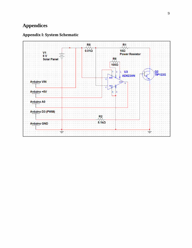
9
Appendices
Appendix I: System Schematic

10
Appendix II: Battery Charger Considerations

11
Appendix III: Battery Charger considerations
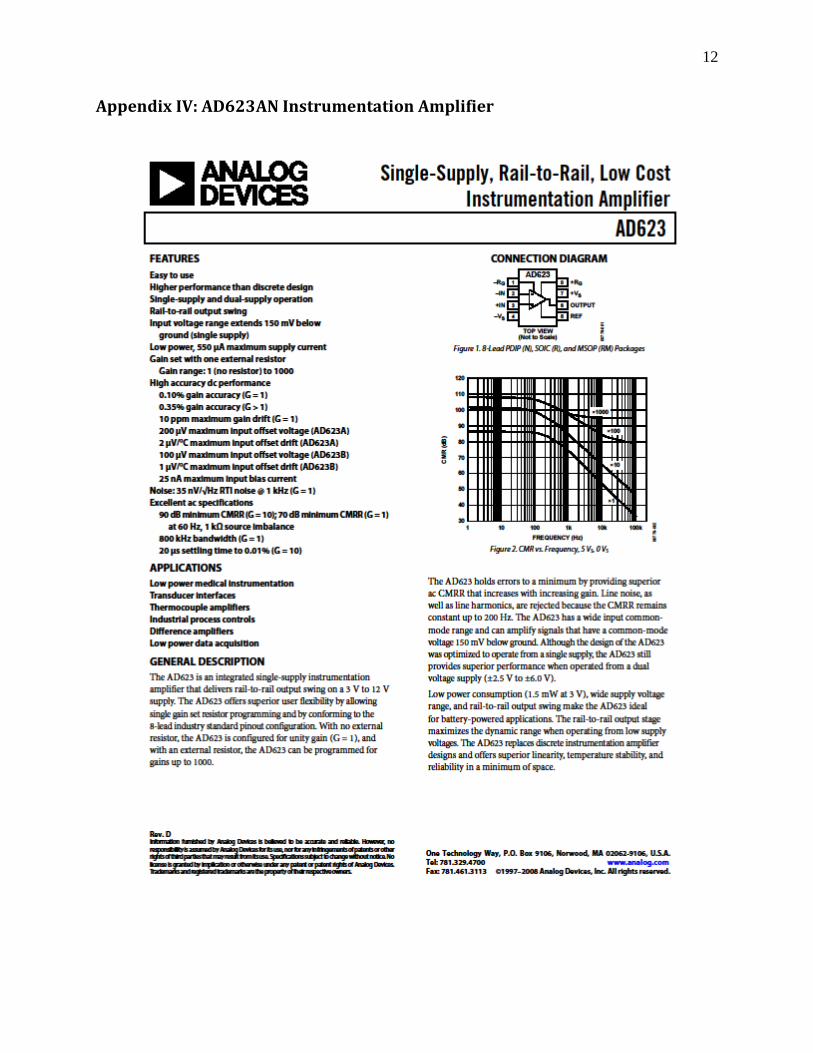
12
Appendix IV: AD623AN Instrumentation Amplifier
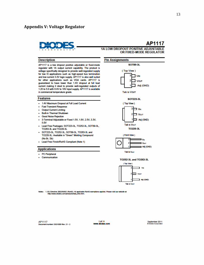
13
Appendix V: Voltage Regulator

14
Appendix VI: Arduino code to use moving average int LOADpin = 3; // Pin that the transistor for the load is connected to
int LOAD = 100; // PWM value for the load
// Recursive Digital Filter Variables
float i4=0; //start all values for current at 20 to avoid them remaining stuck at 0
float i3=0;
float i2=0;
float i1=0;
float i0=0;
float y4=0;
float y3=0;
float y2=0;
float y1=0;
float y0=0;
float a0=0.0048; // values from MATLAB for 4th order, fc = 50 & fs = 8000 (PWM @ 490Hz)
float a1=0.0193; // values multiplied by 2^12 = 4096
float a2=0.0289;
float a3=0.0193;
float a4=0.0048;
float b1=-2.3695;
float b2=2.314;
float b3=-1.0547;
float b4=0.1874;
float I=0;
// LCD Variables:
byte LCD_reset = 12; // reset LCD, clear screen and move to line 0, position 0
byte LCD_line0 = 128; // LCD set line 0, character 0
byte LCD_line1 = 148; // LCD set line 1, character 0
void setup()
Serial.begin(9600);
// reset does not work on all LCDs
Serial.write( LCD_reset ); // reset LCD, clear screen and move to line 0, position 0
delay( 5 ) ; // delay 5 ms after reset
Serial.write( LCD_line0 );
Serial.print( "Solar Panel " );
Serial.write( LCD_line1 );
Serial.print( " " );
pinMode(LOADpin, OUTPUT);
void loop()
int t=millis();

15
analogWrite(LOADpin, LOAD);
// Measure output voltage from AD623
float Vmeas = analogRead(A0)*0.00489; // V
i0=Vmeas;
y0= a0*i0 + a1*i1 + a2*i2 + a3*i3 + a4*i4 - b1*y1 - b2*y2 - b3*y3 - b4*y4;
i4=i3;
i3=i2;
i2=i1;
i1=i0;
y4=y3;
y3=y2;
y2=y1;
i1=i0;
y1=y0;
//recursive digital filter
I=17.9*Vmeas+15.24; // mA
float power = y0*I; //mW
// Arduino takes 40mA
// LCD panel takes 16.6mA
//LCD Controls
// Serial.write( LCD_line0 ); // top line
// Serial.print(V1/1000.0); // print total voltage
// Serial.print(" V ");
// Serial.print(y0); // print total current
// Serial.print(" mA ");
// Serial.write( LCD_line1 ); // second line
// Serial.print(power);
// Serial.print(" W ");
// delay(200);
// Serial Print to computer serial monitor, for data collection
Serial.print(t); // print time
Serial.print(" ");
Serial.print(y0); // print voltage
Serial.print(" ");
Serial.print(I); // print current
Serial.print(" ");
Serial.print(power); // print power
Serial.print(" ");
Serial.println(LOAD); // print power
delay(50);

16
Appendix VII: Maximum Power Point Tracking (MPPT) function
// Maximum Power Point Tracking (MPPT) code
// Reset MPPT variables
float p1=0;
float p2=0;
// Test power @ Higher PWM
LOAD = LOAD + 5;
LOAD = constrain(LOAD,1,255);
analogWrite(LOADpin, LOAD);
delay(10);
for (int n=1; n <= 100; n++)
V1 = analogRead(A0)*4.888; // (mV) upstream of power resistor
V2 = analogRead(A1)*4.888; // (mV) downstream of power resistor
i0=(V1-V2)/R1; // mA
power = i0*V1/1000; //mW
p1 = p1 + power;
// Test power @ lower PWM
LOAD = LOAD - 5;
LOAD = constrain(LOAD,1,255);
analogWrite(LOADpin, LOAD);
delay(10);
for (int n=1; n <= 100; n++)
V1 = analogRead(A0)*4.888; // (mV) upstream of power resistor
V2 = analogRead(A1)*4.888; // (mV) downstream of power resistor
i0=(V1-V2)/R1; // mA
power = i0*V1/1000; //mW
p2 = p2 + power;
// Chose the better direction to move the PWM value to
if (p1 > p2)
LOAD = LOAD + 1;
if (p1 < p2)
LOAD = LOAD - 1;
Final Report Remote Controlled Hovercraft
Arduino processor and battery powered
Richard McClain
Ian Simpson
May 3rd, 2013

ME 445 Final Project
2
Contents Introduction ..................................................................................................................................... 3
Components: complete list of materials/electronics used ............................................................... 4
Physical Components .................................................................................................................. 4
Electrical Components ................................................................................................................ 4
Prototypes: initial designs and iterations ....................................................................................... 6
Electronics: circuit design............................................................................................................... 7
How it works: explanation of design .............................................................................................. 8
Code: how the code works and what it does ................................................................................. 11
Conclusion .................................................................................................................................... 12
Appendix A: source code .............................................................................................................. 13
Appendix B: Circuit Schematic .................................................................................................... 16
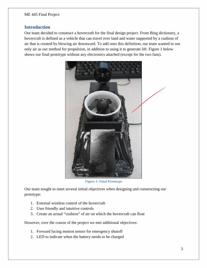
ME 445 Final Project
3
Introduction Our team decided to construct a hovercraft for the final design project. From Bing dictionary, a hovercraft is defined as a vehicle that can travel over land and water supported by a cushion of air that is created by blowing air downward. To add onto this definition, our team wanted to use only air as our method for propulsion, in addition to using it to generate lift. Figure 1 below shows our final prototype without any electronics attached (except for the two fans).
Figure 1: Final Prototype
Our team sought to meet several initial objectives when designing and constructing our prototype:
1. External wireless control of the hovercraft 2. User friendly and intuitive controls 3. Create an actual “cushion” of air on which the hovercraft can float
However, over the course of the project we met additional objectives:
1. Forward facing motion sensor for emergency shutoff 2. LED to indicate when the battery needs to be charged

ME 445 Final Project
4
3. Two “homemade” motor drivers using Mosfets, capacitors, and diodes
The design of the hovercraft was broken into two main sub-systems the physical hovercraft with electrical and structural components and the processing system using the Arduino Uno and source code.
Components: complete list of materials/electronics used Physical Components
1. Gator board – used for the majority of the hovercraft. The bottom piece has a grid of ¼” holes to allow air to escape.
2. Hot glue – used to hold the gator board together 3. Plastic – the plastic is lightweight and focuses the air on the bottom of the board. It is fit
between the lift motor and the bottom board to create a trapezoidal pocket of air, which focuses air on the bottom the craft.
4. Balsa wood – used to create a stable platform for the lift fan to sit.
Electrical Components The majority of the components are electronic. They are as follows.
The circuit components which are shown in Figure 2:
1. PS2 receiver 2. Proximity sensor – Sharp GP2D120XJ00F 3. Arduino Uno 4. Motor Driver
a. Capacitor – 330 μF 50V electrolytic b. Diode – 1N4002 c. Mosfet – 30N06L
5. LED 6. Resistors
a. 2 – 10KΩ b. 1 - 330Ω
7. Battery a. 7.4V 900mAh Tenergy Li-Po

ME 445 Final Project
5
Figure 2: Circuit Components; Top left to right: PS2 receiver, proximity sensor, Arduino Uno
Bottom left to right: Motor driver, resistors, and LED, and Li-Po battery
The large fan used to provide lift to the hovercraft; shown in Figure 3.
Figure 3: Large Fan GWS EDF64 Ducted Fan Unit w/300H Motor
The small fan used to provide thrust (to move the hovercraft forward and laterally); shown in Figure 4.
Figure 4: Small Fan GWS Ducted Fan 2020x3
The PS2 controller, shown in Figure 5, provides a signal to the PS2 receiver shown above.

ME 445 Final Project
6
Figure 5: PS2 Controller
Prototypes: initial designs and iterations During the construction of the hovercraft, there were several major design iterations, which our outlined in Figure 6 below. The first design was a dual slit design show at the top left of Figure 6 below. The concept was that the hovercraft would be most balanced if the lifting force was displaced to the outside edges—much like a pontoon boat or a canoe without riggers—the hovercraft can more easily balance this way. This idea stemmed for our very initial designs (not shown) that used a bag covering the entire bottom of the hovercraft, which was then pumped with air. The issue with these designs was that the largest force of air was centered on the hovercraft creating a bulge in the bag at its center causing the hovercraft to rock back and forth as if it was sitting on half a balloon. This dual slit design shown below instead had two separate bags which filled with air leaving a void space in the center of the hovercraft to eliminate the bulge.
Figure 6: Design Iterations

ME 445 Final Project
7
The dual slit design proved more effective, but the large fan at a lot of trouble keeping the hovercraft elevated and there was significant blow back (air pressure being forced back out the large fan). The next design moved to an air hockey style concept. It featured a main platform where the small fan sat and 1/8” holes placed symmetrically in a grid across the bottom surface. The bottom surface was constructed of gator board and the top of it was covered with plastic with a space for the air coming from the small fan to fill that void space. This design worked much better except that the small fan was not enough to lift the hovercraft and the holes were too small to allow air to escape effectively. (Additionally, several different bottom surfaces were tried including aluminum, plastic, Shurtape (slippery version of duct tape), and gator board). It turns out that gator board has the lowest coefficient of friction.
The third and final design took the best concepts from each subsequent design. It used the air hockey design with the large motor powering it to create that void space between the floor and the hovercraft. The holes were increased from 1/8” to 1/4” in diameter to allow more air to flow out the bottom and a slightly smaller platform base was used; now 5” by 10” instead of the original 6” by 12”.
Electronics: circuit design Figure 7 shows the circuit diagram for the final prototype. The most challenging aspect of the electronics is combining all of these components without a bread board. A breadboard would increase the weight significantly. A small piece of proto board was used in its place to hold of the electrical components in place.
Two individual, single directions, motor drivers were built for the project. Each motor driver combined a MOSFET, a rectifying diode, and a capacitor. PWM from the Arduino was used to control the current flow through the two DC motors. The motors were connected to the batteries positive and the drain side of the MOSFET which allowed the motor to draw current that was limited only by the battery’s capacity rather than the gate to source’s current. A schematic of the circuit can be found in Appendix B.
A lot was learned by building these motor drivers, for example, the sensitivity of MOSFETS to electro-static discharge and the need of parallel capacitance in a circuit that draws high currents for a short period of time. The circuit also uses a simple voltage divider made of two 10KΩ resistors. Measuring between these two resistors provides the Arduino an analog input that can be used to shut the system off if the battery’s voltage droops too low.

ME 445 Final Project
8
Figure 7: Circuit Diagram for Final Prototype
How it works: explanation of design The blow back is initially large when the motor is turned on, because the hovercraft is resting on the floor and the air cannot escape. Once the hovercraft is lifted off the ground, the air escapes from the holes and rushes along the ground and out the sides of the craft—this allows the hovercraft to actually rest on this rushing air causing it to have a tremendous drop in friction as can be seen in Figure 8. Once it is “gliding”, the small fan can easily move the craft by applying force in the opposite direction as shown in Figure 9.
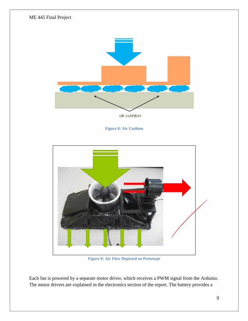
ME 445 Final Project
9
Figure 8: Air Cushion
Figure 9: Air Flow Depicted on Prototype
Each fan is powered by a separate motor driver, which receives a PWM signal from the Arduino. The motor drivers are explained in the electronics section of the report. The battery provides a

ME 445 Final Project
10
maximum 22.5 amp output, but for our purposes discharges at a much slower rate. We used pulse width modulation to control the voltage supplied to each fan; we decided not to run the fans at full speed at the suggestion of our TA. We set our own limit on the fans to 86% of the total voltage. Taking the limit we imposed (0 to 86%) we then mapped the speed of each fan as shown in Figure 10. For the lift fan, we set the range from 50% to 100% of that 86% limit, which is a range of 110 to 220 of the 255 (which would be the full PWM output). The user has control to plus or minus 5 percent of that value, which will be explained below. For the thrust fan, the PWM runs from 0 to 100% of the 0 to 86% duty cycle and also has a resolution of plus or minus 5 percent throughout that range.
Figure 10: PWM and Mapping
The user controls the hovercraft using an aftermarket PlayStation 2 controller, which provides a signal to the PlayStation receiver. The basic controls are shown in Figure 11. The on/off switch to the controller is at the bottom of the controller between the two joysticks. The start button turns the lift fan on to 50% and the select switch shuts everything off (including the thrust fan if it is on). The left and right bumpers (the lower two) increase and decrease the speed of the lift fan by minus or plus 5% respectively as shown in Figure 10.
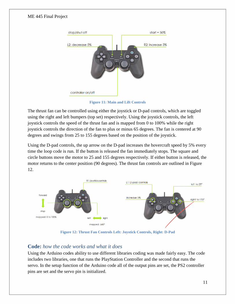
ME 445 Final Project
11
Figure 11: Main and Lift Controls
The thrust fan can be controlled using either the joystick or D-pad controls, which are toggled using the right and left bumpers (top set) respectively. Using the joystick controls, the left joystick controls the speed of the thrust fan and is mapped from 0 to 100% while the right joystick controls the direction of the fan to plus or minus 65 degrees. The fan is centered at 90 degrees and swings from 25 to 155 degrees based on the position of the joystick.
Using the D-pad controls, the up arrow on the D-pad increases the hovercraft speed by 5% every time the loop code is run. If the button is released the fan immediately stops. The square and circle buttons move the motor to 25 and 155 degrees respectively. If either button is released, the motor returns to the center position (90 degrees). The thrust fan controls are outlined in Figure 12.
Figure 12: Thrust Fan Controls Left: Joystick Controls, Right: D-Pad
Code: how the code works and what it does Using the Arduino codes ability to use different libraries coding was made fairly easy. The code includes two libraries, one that runs the PlayStation Controller and the second that runs the servo. In the setup function of the Arduino code all of the output pins are set, the PS2 controller pins are set and the servo pin is initialized.

ME 445 Final Project
12
When the code enters the loop function three functions are called continuously. The first is the buttsorsticks function. This function looks for either the R1 or L1 buttons to be pressed to set the direction control to with buttons or joysticks. The second function is the lift function. This function looks for an input from the start button. Once the start button is pressed a run variable is switched to on and the lift motor is turned on with an initial thrust. This function then continues looking for the L2 and R2 buttons in order to increase or decrease this lift. Finally the third loop is the thrust fan loop. This loop uses the result of the buttsorsticks function to run a switch case. This switch case either looks for inputs from the D-pad or the joysticks. Theses inputs are then mapped to a speed and output as PWM to the motor. The inputs for turning the servo are also looked for in the thrust function. These inputs are mapped to a degree position and output to the servo pin.
Also included in the loop function is an if statement that is used as an emergency stop feature. This if statement is triggered when either select is pressed, the wall function is triggered, or the battery voltage function returns a low value. The wall function looks at the analog input of the proximity sensor and switches its Boolean state to true if the sensor is closer than 10 cm. The batter voltage reads an analog input and returns a number that correlates to the voltage of the battery.
Conclusion In conclusion, are hovercraft proved to be a unique and challenging problem. Unlike the Zumobots or other projects where the platform or basic project is easy—a controllable robot—our “basic” project was our project. Just achieving lift and creating a cushion of air for our hovercraft proved to be the biggest challenge we faced. We learned that weight is everything; any little piece of plastic casing, balsa wood, or wiring that was not necessary had to come off. We learned that there is a big difference between having your hovercraft float on that air cushion where the friction is almost zero and a hovercraft that has its back end still dragging along the ground; much harder to control the latter. We learned that there is a right way and a wrong way to mount a fan—running it in reverse does not generate anywhere nears the same volume and speed of air. And lastly, we learned that simple code is a lot easier to decode—so keep it simple. At the conclusion of our project, we created a hovercraft capable of easy and intuitive motion using a wireless controller; mounted with a distance sensor to stop the hovercraft before it crashes into any obstacles. If a team were to continue our project next year I would like to see them build a larger hovercraft. They would have to add additional fans to achieve the required lifting force, but it would allow them better control. Two thrust fans for better turning and the ability to run in revers and better stabilization of the platform with two lifting fans. With a better base, they could mount additional sensors or electronics. We looked into having a ramp that dropped down and let out a little RC car or tank similar to how it might work with an operational hovercraft in the armed forces today. Whatever they do with our project though, I hope they learned as much as we did.

ME 445 Final Project
13
Appendix A: source code #include "PS2X_lib.h" //for v1.6 PS2X ps2x; // create PS2 Controller Class #include "Servo.h" Servo backmotor; // create servo object to control a servo int error = 0; //PS2 variable byte type = 0; //PS2 variable byte vibrate = 0; //PS2 variable int initiallift=50; //intial lift boolean run = false; //run variable - false is off, true is on int liftspd = 0; //lift speed int dircntrler = true; //use D-pad or Sticks int M1 = 5; //Lift fan pin int M2 = 6; //Thrust fan pin int battLED = 2; // Pin for battery LED int servoint = 100; // Servos intial point int deg = 100; // Used to turn back motor int Tintspd = 20; // Initial Thrust speed int Tspeed = 0; // Thrust motor speed void setup() Serial.begin(57600); // PS2 used 57600 backmotor.attach(4); // attaches the servo on pin 22 to the servo object backmotor.write(servoint); // set the servo to the mid point // Set pins pinMode(M1, OUTPUT); pinMode(M2, OUTPUT); pinMode(battLED,OUTPUT); digitalWrite(battLED,HIGH); // Turn LED on error = ps2x.config_gamepad(13,11,10,12, false, false); //setup pins and settings:
GamePad(clock, command, attention, data, Pressures?, Rumble?) check for error type = ps2x.readType(); //Reads type of PS2 Controller switch(type) case 0: //Serial.println("Unknown Controller type"); break; case 1: //Serial.println("DualShock Controller Found"); break; case 2: //Serial.println("GuitarHero Controller Found"); break; void loop() if(error == 1) //skip loop if no controller found return; else //DualShock Controller ps2x.read_gamepad(false, vibrate); if(ps2x.ButtonPressed(PSB_SELECT) || battvolt() <= 25 || wall()) //Turn off motors and change run variable to false LiftFan(0); ThrustFan(0); run=false; liftspd=0; dircntrler=0; buttsosticks(run,ps2x.ButtonPressed(PSB_L

ME 445 Final Project
14
1),ps2x.ButtonPressed(PSB_R1)); // Function that decides whether to read stick input or D-pad input lift(initiallift,ps2x.ButtonPressed(PSB_START),ps2x.ButtonPressed(PSB_R2),ps2x.ButtonPressed(PSB_L2)); // Function that determines speed of the lift fan thrustmotor(dircntrler); // Function that determines speed of the thrust fan //Serial.println(dircntrler); // used to debug delay(50); void buttsosticks (boolean a, boolean b, boolean c) // Used to determine whether to use joysticks or the D-pad if (a) if (b) dircntrler=1; if (c) dircntrler=2; else dircntrler=0; void LiftFan(int S) int spdL = S*220/100; analogWrite(M1, spdL); void ThrustFan(int S) int spdT = S*220/100; analogWrite(M2,spdT);
int lift(int x, boolean a, boolean y, boolean z) if (a) //start is pressed liftspd=x;// m1 speed to intial lift run=true;//run variable is true ThrustFan(Tintspd); LiftFan(liftspd); if (y && liftspd<100 && run) liftspd=liftspd+5;//when r2 is pressed lift increased by 10 if run variable true ThrustFan(Tintspd); LiftFan(liftspd); if (z && liftspd>0 && run) liftspd=liftspd-5;//when r2 is pressed lift decreased by 10 if run variable true ThrustFan(Tintspd); LiftFan(liftspd); //Serial.println(liftspd); int thrustspd(int x, boolean a) if (a && Tspeed<100) Tspeed=Tspeed+5; else Tspeed = x; return Tspeed; void rudd(boolean b, boolean a) if(a && deg > 25) deg=deg+5; backmotor.write(deg);

ME 445 Final Project
15
else if(b && deg < 155) deg=deg-5; backmotor.write(deg); else deg=servoint; backmotor.write(deg); int sticks(int a, int b) int fspd; if (a>125) // If the stick is pushed back set fan to Initial Thrust speed fspd=Tintspd; else fspd=map(a,0,128,100,Tintspd); // map stick movement to fan speed deg=map(b,0,255,165,35); // map stick movement to servo position ThrustFan(fspd); // Run thrust fan at set speed backmotor.write(deg); // Turn motor to set position //Serial.println(turn); void thrustmotor(int a) switch (a) case 1: rudd(ps2x.Button(PSB_RED),ps2x.Button(PSB_PINK)); int Tspd=thrustspd(20,ps2x.Button(PSB_PAD_UP));
if(ps2x.Button(PSB_PAD_UP)) ThrustFan(Tspd); else ThrustFan(Tintspd); break; case 2: sticks(ps2x.Analog(PSS_LY),ps2x.Analog(PSS_RX)); break; int battvolt() float analogBV = analogRead(A1); float realBV = analogBV*50/1023; if (realBV < 25) digitalWrite(battLED,LOW); else digitalWrite(battLED,HIGH); //Serial.println(realBV); return realBV; boolean wall() boolean W = false; int distance = 0; distance = analogRead(A0); //Serial.println(distance); if (distance > 150) W = true; else W = false; return W;

ME 445 Final Project
16
Appendix B: Circuit Schematic

1
PENNSTATE Department of Engineering Science
Group 14 Final Report
Automatic Meat Smoker Controller
Date: May 3, 2013
Mike Pelino Nathan Roll

2
Executive Summary We have developed a device and program that will automatically control the pit temperature of meat smoker while the meat is cooking. The user will enter both their desired pit and meat temperature and the smoker will achieve and hold this pit temperature while waiting for the meat to finish cooking. Once the meat is finished, the controller’s LCD displays flashes and waits for the user to acknowledge and remove the food. The device is set up so that the user enters their temperatures on a keypad. Then the program controls the smoker vents to help reach the pit temperature. The vents are controlled by servos. These servos rotate based on the actual versus desired pit temperature. The controller also features two temperature probes, one meat thermistor that records the internal temperature of the meat and one type K thermocouple that records the pit temperature. The meat probe is what signals the program to stop running once the desired internal temperature has been reached. There is limited user interaction with the controller after entering the desired temperatures. The current, filtered meat and pit temperatures are constantly displayed so the user can check on progress of their food. They can also check what they entered the desired temperatures to be, and can change them if necessary. Finally, they can turn on the backlight of the LCD if the current temperatures are too difficult to read.

3
Table of Contents Executive Summary ........................................................................................................................ 2
1.0 Introduction ............................................................................................................................... 4
1.1 Motivation ............................................................................................................................. 4
2.0 Hardware/Circuitry ................................................................................................................... 4
2.1 Bill of Materials .................................................................................................................... 4
2.2 Jameco Keypad ..................................................................................................................... 5
2.3 LCD Display ......................................................................................................................... 5
2.4 Servo ..................................................................................................................................... 6
2.5 Temperature Probes .............................................................................................................. 7
2.5.1 Type K Thermocouple Probe .................................................................................... 7
2.5.2 Thermister Meat Probe ............................................................................................. 7
3.0 Software .................................................................................................................................... 9
4.0 Discussion ................................................................................................................................. 9
5.0 Conclusions ............................................................................................................................. 11
Appendix A - Ardunio Code ......................................................................................................... 12
Appendix B - Circuit Diagrams .................................................................................................... 21
Appendix C - Thermister Testing Results .................................................................................... 23
Appendix D - Hardware Data Sheets ............................................................................................ 26

4
1.0 Introduction The final project of ME 445 tasked our group with using mechatronics to create some type of interesting device. Our group ultimately settled on making a controller to command the vents on a meat smoker in order to more accurately control the temperature of the cooker. We chose this project because it incorporated several topics that were discussed in class and in our labs all the while allowing us to expand upon those discussions. Eventually, we were able to harness several different types of technology to create a device that used upon each individual part in unison to create a controller. 1.1 Motivation The main motivation for this project was to create something useful after the class was completed. We did not want to develop something that we would never touch again after graduation. This lead us to the meat smoker controller, as both group members are very interested in food and grilling. Also, one member already owns a smoker and commented on how difficult it is to control the vents and keep the internal temperature constant. Since smoking is usually a low and slow process, it is not efficient (and usually not possible) to sit next to the smoker for hours on end to monitor the temperature and adjust the vents accordingly. Therefore, the creation of an automated process would help to produce top quality food without having to waste an entire day sitting by your smoker. Also, the controller allows for the meat temperature to be read and a final display when your meat has reached it final temperature.
2.0 Hardware/Circuitry 2.1 Bill of Materials
Units Item Vendor Approx. Cost
1 Arduino Uno Jameco $30.00
3 HiTec HS-‐311 Standard Servos Servocity $8.00
1 Type K Thermocouple Instr Rm. -‐
1 AD 595 Type K Thermocouple Amplifier SparkFun $18.00
1 Recycled Thermister temp Probe -‐ -‐
1 Keypad Jameco $10.00
1 LCD Display Amazon $22.00
1 Wood Scrap Instr Rm. -‐
3 10 KΩ Resistor Paralax $0.20
Total $89.00

5
For the smoker controller we used an Arduino Uno as the brains of the unit. To it, we attached a type K thermocouple that will be used to measure the temperature inside of the pit. A thermistor, in the form of an old out of calibration meat probe, will be used to measure the temperature of the meat inside of the smoker. The Arduino interprets the data measured by the thermistor and thermocouple and uses it along with user input from a keypad to control 3 servos. Essentially, the user inputs their desired pit temperature on the keypad and the controller takes care of maintaining that temperature by opening and closing the smoker vents. If the temperature of the pit needs raised, the Arduino will tell the smoker to open the vents, which allows more airflow into the smoker and raises the smoker temperature. If the temperature inside the pit is too low, then the Arduino closes the vents to cut the charcoal off from oxygen, lowering the temperature of the pit. The servos are mounted on the vents using fabricated metal strips and secured to the ground using a stand made from scrap wood from the Instrument Room. We also incorporated an a LCD into our design to output the current pit and meat temperature along with the user inputted temps. 2.2 Jameco Keypad The only piece of hardware that will receive user interaction is the keypad. For this project we chose the Jameco keypad. The biggest advantage to this keypad was the extra four alphabet keys. We were able to use these keys to allow the user to initiate the prompts for final meat and pit temperature. The keypad is wired directly into the Arduino with 8 separate digital pins. We soldered an 8 pin SIP into the keypad connection and then ran a grouped set of 8 wires to the Aduino. Each pin corresponds to either a row or column, and when a key is pressed the combination of two inputs results in the program recognizing the keystroke. To implement this feature on the Arduino, we first had to download a separate ‘keypad’ library from the Internet, since it is not one of the standard libraries provided by Arduino. This library simplifies the integration of the keypad and eliminates redundant coding from program to program. After initializing the location of characters on the keypad, and which pins corresponded to which rows and columns, the keypad was ready to use. The only other caveat of using the keypad was that it sent characters to the Arudino, whether the character was a number or letter. This fact forced us to convert characters to numbers whenever the user was entering their meat and pit temperatures. Since each character was taken in individually, the first and second numbers had to be multiplied accordingly to put them in the hundreds and tens place. 2.3 LCD Display The LCD Display is the main visual interaction with the user. While the user interacts with the keypad, they read what the program wants and what they entered on the LCD. The LCD used for the project was the Sainsmart I2C Serial 2004 Display. This is a 20-column and 4-row display. A very nice feature of the display is the I2C adapter on the back. This reduces the output

6
pins to only four and allows for easy connection to the Arduino. Two of the pins are VCC and GND and were wired directly into the corresponding Arudino inputs. The other two were SDA and SCL, and they were also wired into their corresponding Arduino inputs. Since we used an Arduino Uno, we had to add two 10K pull-up resistors to these connections in order for the LCD to display properly. One resistor ran from VCC to SDA and the other from VCC to SCL. Insulation was wrapped around the resistors to prevent the wires from crossing and touching. The next thing we had to do to ensure operation was to download another library from the Internet, since Arduino’s default Liquid Crystal library is not compatible with our display. The best current LCD library is F. Malpartida’s. This library allows for easy integration of the I2C display with the Arduino. It takes care of assigning all of the pins and connections of the adaptor and really helps out the programmer. After downloading a short sample code that showed how to initialize the display and operate the backlight within the program, we only needed to determine the I2C address to be operational. This address was provided by Sainsmart to be 0x3F. The LCD we used was perfect for our operation. The 4 rows were perfect and made for an aesthetically pleasing user interface. We were also able to always display the current meat and pit temperatures on the bottom two lines. Nothing got squeezed or cut off and was spaced nicely. Also, a backlight can be turned on and off to allow for both easy reading and power conservation. 2.4 Servo To physically move the vents on the smoker, we chose to use servos mounted to the vents to turn them open or closed. We used three of the HiTec HC-311 Standard servos. The servos are held in position via wood stands. We used these servos because they were available to us in the lab already and satisfied our needs. The servos are instructed by the Ardunio to move to certain positions based on the difference in the pit temperature and the user inputted temperature. To move the servos, the program enters a function that calculates the difference between the desired and actual temperature. The movement of the servos also must be constrained between 0° and 48° because that is how far the vent covers rotates from fully open to fully closed. If the difference in temperature is greater than 40°F, the servos move the fully opened position. They will remain there until the pit temperature is less than 40°F cooler than the desired temperature. After this, the servo closes 1° for each 1°F the pit temperature moves towards its goal. Since the servo library is provided with Arduino, it was relatively simple to move the servos into proper position. The difference in temperature, if within -10°F and 40°F, is then added to ten and written directly to the servo as the position it should be in. This one for one movement makes the servo respond perfectly to each individual change in temperature.

7
2.5 Temperature Probes
2.5.1 Type K Thermocouple Probe To monitor the smoker temperature we used a type K thermocouple obtained from the instrument room. To amplify the thermocouple's signal we used an AD595 Type K Thermocouple Amplifier that amplifies its signal. The output of the AD595 is read by an Arduino analog input as a number between 0 and 1023, which gets converted to a voltage by dividing by 1024 and multiplying by 5V. The converted voltage can then be used to calculate the temperature by multiplying it by 10mV/C°. A schematic of how it is wired into the Arduino can be seen below in Figure 2.1.
Figure 2.1: Thermocouple Wiring Schematic.
2.5.2 Thermistor Meat Probe To measure the temperature of the meat in the smoker, we recycled the use of a seemingly broken meat thermometer probe seen below in Figure 2.2. We suspected that the probe (which by the price and type was a thermistor) needed to be recalibrated so we set up an experiment to re-calibrate it. The probe was set in a cup of near boiling water along with another temperature reading device to get a true reading of the temperature of the water. As the water cooled inside of the cup, we measured the resistance across the lead wires of the probe and recorded it along with the true temperature of the water. After the test, we converted the measured resistance values to voltage values through a voltage divider. A schematic of circuit and the equation used to calculate the voltage can be seen below in Figure 2.3 and Equation 2-1. We used a 10 KΩ resistor in series with the thermistor because it provides the greatest accuracy near the middle of
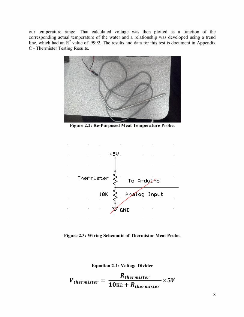
8
our temperature range. That calculated voltage was then plotted as a function of the corresponding actual temperature of the water and a relationship was developed using a trend line, which had an R2 value of .9992. The results and data for this test is document in Appendix C - Thermister Testing Results.
Figure 2.2: Re-Purposed Meat Temperature Probe.
Figure 2.3: Wiring Schematic of Thermistor Meat Probe.
Equation 2-1: Voltage Divider
𝑽𝒕𝒉𝒆𝒓𝒎𝒊𝒔𝒕𝒆𝒓 = 𝑹𝒕𝒉𝒆𝒓𝒎𝒊𝒔𝒕𝒆𝒓
𝟏𝟎𝐊Ω + 𝑹𝒕𝒉𝒆𝒓𝒎𝒊𝒔𝒕𝒆𝒓 ×𝟓𝑽

9
3.0 Software
The purpose of our controller is to hold the temperature inside the smoker constant while waiting for the meat to reach the user’s final goal temperature. After properly inserting the pit and meat probes, the user enters their desired final meat temperature (prompted for by striking ‘A’) and pit temperature (prompted for by striking ‘B’). This is all they have to do; the computer takes care of the rest. The Arduino constantly reads the pit and meat temperatures and outputs them to the LCD display. Since the temperatures can vary from reading to reading and many readings are being taken over the course of operation, a filter is used to help eliminate big spikes. The filter takes a weighted average of the running average and the newly read temperature, with a 99% emphasis on the running average. This filter also ensures that the controller does not stop because the meat probe got one hot reading or experienced noise while in reality the meat is nowhere near done. This allows the user to come by and check on their progress at any time. The program is designed to leave the smoker vents fully open until the pit temperature is within 40°F of the desired value. As the pit temperature continues to climb, the Arduino signals the servos to close the vents one degree for each degree the temperature moves closer to the goal, up to 8 degrees of overshoot. The overshoot was designed to allow for the vents to remain slightly cracked if the pit temperature was exactly as desired. This small crack allows for gentile airflow into the pit to help the temperature remain constant at its target. As the Arduino controls the pit temperature with the vents, it is also monitoring the meat temperature. This is the final goal of the program since your food is ready when the meat is properly cooked, not just when your pit reaches temperature. The current meat temperature is continuously compared with the goal meat temperature. Once this temperature is reached, the LCD begins to flash and report that your food is ready. It will continue to flash until the user strikes any key. This starts the loop again and the Arduino waits for the user to command it to ask for a desired meat and pit temperature, therefore starting the program again. There is very limited user interaction with the program while it is running. While the user can go back and change the goal temperatures (by striking ‘A’ or ‘B’ on the keypad), they will most likely choose not to do so. The main thing the user can do is confirm where they set the meat and pit (done by pressing ‘C’ and ‘D’, respectively) to reach. Finally, the user can turn on the LCD backlight by striking ‘0’ so they can read the current pit and meat temperature. Turning on the backlight would be the most used feature, and it is designed to remain on for three seconds after the user presses the button. Once the backlight is off, the smoker controller continues operation. We designed the smoker for minimal interaction because we wanted it to be as easy as possible for the user to prepare their food. 4.0 Discussion We both learned an incredible amount about mechatronics from this final project. Neither group member had any experience with Arduino before this class. Based on where we were at the beginning of the class, I am impressed that we developed a smoker controller. The biggest thing we learned on this project was Arduino programming. Coming in to this class, the only
10
experience we had was FORTRAN. The use of the keypad and LCD screen basically forced us to scour the Internet for data sheets and information on how to program them. This also led to the discovery of already developed libraries that simplify, and most importantly shorten, this process. These libraries help to initialize the devices and "clean up" the final program. While we only needed two of these libraries (Keypad and Malpartida’s LCD), it was interesting to see all of the different ones out there. The knowledge of these libraries will be useful should we ever program in Arduino again. Finally, the Arduino forums were incredibly helpful. Since most people had the same problems we did, they posted solutions and sample code that helped us along the way.
Like most projects, this one had its stumbling blocks and pitfalls. One of the hardest things to do was getting the keypad to read and record the user’s strokes. The Internet was the key to solving this problem, as it suggested the use of an 'if' statement and then ‘case’s within it. First, the Arudino sets a variable to look for a key to be pressed. Once pressed, the if-case loop is entered. The tricky part of this set-up was to use the ‘switch’ command to allow the pressed key to be used in the case structure. Then, based on the stroke it acts accordingly. The next tough part was receiving the user’s temperature inputs. This was done in a function. The function also waits for a key to be pressed before recording the value. This same phrase had to repeated three times for each of the three digits entered. First, we tried a while loop, but that failed as a long key press would double the value and a lackadaisical one would be skipped. We developed this solution with Mike and actually posted our code online because someone on the forum was having the same problem as us. This was very gratifying as we were able to help others with something we are just becoming comfortable with.
The LCD was not too difficult to program, but took a lot of searching to get working, especially since the default Liquid Crystal Library was not compatible and the LCD manufacturer provided no help on their website. This again forced us to the Arduino forums. After much searching and reading we finally found some sample code and an explanation. We were told to download Malpartida’s library, which would save us a ton of time and hassle. The final obstacle we encountered was with the probe and thermocouple. As noted in the report above, the probe was broken and was recalibrated with the help Excel. However, reading the temperature was not the main problem. Since these thermometers are very sensitive, even the slightest bit of noise can interfere with their reading. Noise was extremely troublesome when trying to get accurate meat and pit temperature. Just one small spike for a millisecond would totally throw off our program and cause it to react undesirably. This was solved with the use of filter. The filter weights the running average and current reading, allowing for a much smoother temperature reading from loop to loop.

11
5.0 Conclusions Overall, we are both very pleased with our final project. We have both gained incredible knowledge in the field of mechatronics and now have a useable, tangible product to take with us. We also have every intention of using our project over the summer at cookouts. This was our goal; to have something we can still use after graduation, and we achieved it. We have also learned how to read and decipher data sheets, how to program an Arudino, and how to interface our Arduino with different components. This knowledge will definitely help us in both our careers and personal lives. We are both impressed with how much we have learned and are thankful we took this class and are pleased to be taking home a useable project.

12
Appendix A - Arduino Code

13
//Program: Smoker Control //By: MP + NR //Include KeyPad Library #include <Keypad.h> //Include Servo Movement Library #include <Servo.h> //Include Malpartida's LCD libraries #include <Wire.h> #include <LCD.h> #include <LiquidCrystal_I2C.h> //Set up Keypad const byte ROWS = 4; //Four Rows const byte COLS = 4; //Four Columns int i = 0; //Counting integer //Store pressed numbers after conversion volatile long int digitOne; volatile long int digitTwo; volatile long int num; volatile long int digitThree = 0; char digitOneChar; char digitTwoChar; char digitThreeChar; char keys[ROWS][COLS] = '1','2','3','A', '4','5','6','B', '7','8','9','C', '*','0','#','D' ; // Connect keypad ROW1, ROW2, ROW3 and ROW4 to these Arduino pins. byte rowPins[ROWS] = 9, 2, 3, 5; //connect to the row pinouts of the keypad // Connect keypad COL1, COL2, COL3, and COL4 to these Arduino pins. byte colPins[COLS] = 4, 6, 7, 8; //connect to the column pinouts of the keypad Keypad keypad = Keypad(makeKeymap(keys), rowPins, colPins, ROWS, COLS); //End Keypad setup //Set up LCD Display #define I2C_ADDR 0x3F // Define I2C Address where the PCF8574A is #define BACKLIGHT_PIN 3 #define En_pin 2 #define Rw_pin 1 #define Rs_pin 0

14
#define D4_pin 4 #define D5_pin 5 #define D6_pin 6 #define D7_pin 7 LiquidCrystal_I2C lcd(I2C_ADDR,En_pin,Rw_pin,Rs_pin,D4_pin,D5_pin,D6_pin,D7_pin); //End LCD setup //Declare Variables //Variable for user temp input float UserPitTemp = 350; //Variable for actual pit temp float PitTempNow = 30; //Variable for actual pit temp float PitTemp; //Variable for user meat temp float UserMeatTemp = 150; //Variable for actual meat temp float MeatTempNow; //Variable for running average of meat temp float MeatTemp = 65; //Variable to indicate temp to store int TempType; //Create servo objects to control servos. We are using three servos Servo pitServo1; Servo pitServo2; Servo pitServo3; //Set pins to read temps int meatPin = 0; int pitPin = 1; void setup() //Make probe's output an input pinMode(meatPin, INPUT); pinMode(pitPin, INPUT); //Attach Servos to pins pitServo1.attach(10); pitServo2.attach(11); pitServo3.attach(12); //Set up the LCD's number of rows and columns: lcd.begin (20,4); void loop() char key = keypad.getKey();

15
//Get/Read temps. Only do this when commanded by user on keypad if (key != NO_KEY) switch (key) //Ask user for desired meat temperature case 'A': digitOneChar = NO_KEY; digitTwoChar = NO_KEY; digitThreeChar = NO_KEY; TempType = 1; //Indicate Meat Temp //Activate LCD lcd.setBacklightPin(BACKLIGHT_PIN,POSITIVE); //Turn on backlight lcd.setBacklight(HIGH); lcd.clear (); //Clear screen and go home lcd.print("Desired Meat Temp?"); //Get numbers pressed getNumbers(); //Turn off LCD light delay(3000); lcd.setBacklightPin(BACKLIGHT_PIN,POSITIVE); lcd.setBacklight(LOW); break; //Ask user for desired pit temperature case 'B': digitOneChar = NO_KEY; digitTwoChar = NO_KEY; digitThreeChar = NO_KEY; TempType = 0; //Indicate Pit Temp //Activate LCD lcd.setBacklightPin(BACKLIGHT_PIN,POSITIVE); //Turn on backlight lcd.setBacklight(HIGH); lcd.clear (); //Clear screen and go home lcd.print("Desired Pit Temp?"); //Get numbers pressed getNumbers(); //Turn off LCD light delay(3000); lcd.setBacklightPin(BACKLIGHT_PIN,POSITIVE); lcd.setBacklight(LOW);

16
break; //Print out entered Meat Temp. Used for user confirmation if wanted. case 'C': //Clear and Activate LCD lcd.setBacklightPin(BACKLIGHT_PIN,POSITIVE); //Turn on backlight lcd.setBacklight(HIGH); lcd.clear (); //Clear screen and go home //Print User's Desired Meat Temp lcd.print("Desired Meat Temp:"); lcd.setCursor(0, 1); //Go to next line lcd.print(UserMeatTemp); lcd.setCursor(7, 1); lcd.print((char)223); lcd.print("F"); //Turn off LCD light delay(1000); lcd.setBacklightPin(BACKLIGHT_PIN,POSITIVE); lcd.setBacklight(LOW); break; //Print out entered Pit Temp. Used for user confirmation if wanted. case 'D': //Clear and Activate LCD lcd.setBacklightPin(BACKLIGHT_PIN,POSITIVE); //Turn on backlight lcd.setBacklight(HIGH); lcd.clear (); //Clear screen and go home //Print User's Desired Meat Temp lcd.print("Desired Pit Temp:"); lcd.setCursor(0, 1); //Go to next line lcd.print(UserPitTemp); lcd.setCursor(7, 1); lcd.print((char)223); lcd.print("F"); //Turn off LCD light delay(1000); lcd.setBacklightPin(BACKLIGHT_PIN,POSITIVE); lcd.setBacklight(LOW);

17
break; //Turn On LCD Backlight for 5 seconds case '0': //Turn on LCD for 3 seconds lcd.setBacklightPin(BACKLIGHT_PIN,POSITIVE); //Turn on backlight lcd.setBacklight(HIGH); delay(3000); lcd.setBacklightPin(BACKLIGHT_PIN,POSITIVE); lcd.setBacklight(LOW); break; //Read meat temperature //Convert from voltage to degrees F. This equation was derived experimentally using Excel. //The results are in the final report MeatTempNow = (((analogRead(meatPin) * 5.0 / 1024.0) - 5.6724) / -0.0223); //Determine running average of meat temp. This helps to filter spikes in temp due to noise MeatTemp = .99 * MeatTemp + .01 * MeatTempNow; //Compare to see if desired meat temp is reached. This is the ultimate goal. // Will also work for one degree over to give user extra time to notice if (int(MeatTemp) == int(UserMeatTemp) || int(MeatTemp) == int(UserMeatTemp + 1)) //Flash LCD that food is done lcd.setBacklightPin(BACKLIGHT_PIN,POSITIVE); //Turn on backlight lcd.setBacklight(HIGH); lcd.clear (); //Clear screen and go home lcd.print("Food is Ready!"); lcd.setCursor(0, 2); lcd.print("Food is Ready!"); delay(800); lcd.setBacklightPin(BACKLIGHT_PIN,POSITIVE); //Turn on backlight lcd.setBacklight(LOW); delay(200); //Read pit temperature //Convert from voltage to degrees F. //This uses an AD595 Type K Thermocouple PitTempNow = (analogRead(pitPin) * 5.0 / 10.24) * 1.8 + 32 + 20; //Add 20 to recalibrate //Determine running average of meat temp

18
PitTemp = .99 * PitTemp + .01 * PitTempNow; //Compare to see if desired meat temp is reached. If not equal, move servo to inc/dec air flow if (PitTemp != UserPitTemp) pitServo1.write(PitControl(PitTemp, UserPitTemp)); //Move Servo 1 the desired number of degrees pitServo2.write(PitControl(PitTemp, UserPitTemp)); //Move Servo 2 the desired number of degrees pitServo3.write(PitControl(PitTemp, UserPitTemp)); //Move Servo 3 the desired number of degrees //Consistently Print Pit and Meat Temp on LCD display lcd.clear(); //Meat lcd.setCursor(0,2); lcd.print("Meat:"); lcd.setCursor(5,2); lcd.print(MeatTemp); //Pit lcd.setCursor(0,3); lcd.print("Pit:"); lcd.setCursor(5,3); lcd.print(PitTemp); //Delay for effect delay(300); //Pit Control Function. This function takes in Actual and Desired Pit Temp. //It then compares them and turns the difference into a position for the servo to be in (in degrees) float PitControl(float Actual, float Desired) //Return value in degrees. This is the position the servo will move to. float Diff = Desired - Actual; //Contrain servo movement to 0 to 48 degrees. This is the maximum motion of the smoker vents if (Diff < -10) //If temp is over 10 deg too hot, want vents to be fully closed to facilitate cool down return 0; else if (Diff > 40) //If temp is over 40 deg too cold, put vents fully open to facilitate heat up return 48; else

19
//Set servo angle 10 degress away from temp difference. This is done so that the vents are open 10 degrees // when the temp is spot on. This will allow for moderate airflow and temperature stabilization. return Diff + 10; //Function to read inputted numbers void getNumbers() lcd.setCursor (0, 1); //Go to next line lcd.cursor(); //Turn on LCD cursor for asthetics while (digitOneChar == NO_KEY) digitOneChar = keypad.getKey(); lcd.print(digitOneChar); while (digitTwoChar == NO_KEY) digitTwoChar = keypad.getKey(); lcd.print(digitTwoChar); while (digitThreeChar == NO_KEY) digitThreeChar = keypad.getKey(); lcd.print(digitThreeChar); //Convert the char to int digitOne = digitOneChar - 48; digitTwo = digitTwoChar - 48; digitThree = digitThreeChar - 48; //Multiplying each digit so as to form a 3 digit number hundreds + tenths + ones digitOne = digitOne * 100; digitTwo = digitTwo * 10; //Output entered temp to user if (TempType == 1) UserMeatTemp = digitOne + digitTwo + digitThree; lcd.setCursor(0,3); lcd.print("You entered:"); lcd.setCursor (13, 3); lcd.print(UserMeatTemp);

20
else UserPitTemp = digitOne + digitTwo + digitThree; lcd.setCursor(0,3); lcd.print("You entered:"); lcd.setCursor (13, 3); lcd.print(UserPitTemp);

21
Appendix B - Circuit Diagrams

22
Figure B.1: Master Wiring Diagram

23
Appendix C - Thermister Testing Results
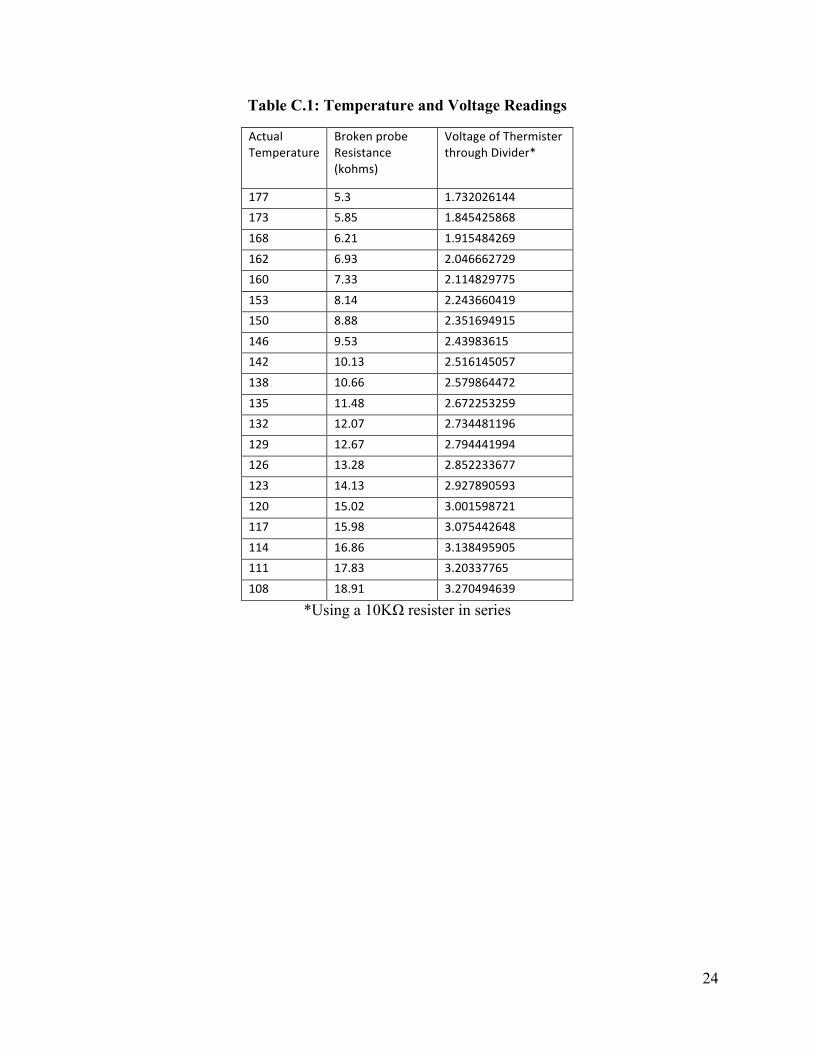
24
Table C.1: Temperature and Voltage Readings
Actual Temperature
Broken probe Resistance (kohms)
Voltage of Thermister through Divider*
177 5.3 1.732026144 173 5.85 1.845425868
168 6.21 1.915484269
162 6.93 2.046662729 160 7.33 2.114829775
153 8.14 2.243660419 150 8.88 2.351694915
146 9.53 2.43983615 142 10.13 2.516145057
138 10.66 2.579864472
135 11.48 2.672253259 132 12.07 2.734481196
129 12.67 2.794441994 126 13.28 2.852233677
123 14.13 2.927890593
120 15.02 3.001598721 117 15.98 3.075442648
114 16.86 3.138495905 111 17.83 3.20337765
108 18.91 3.270494639
*Using a 10KΩ resister in series

25
Figure C.1: Chart showing Voltage vs. Temperature for the Broken Probe in a Voltage Divider Circuit with a 10 KΩ Resistor.
y = -‐0.0223x + 5.6724 R² = 0.99923
0
0.5
1
1.5
2
2.5
3
3.5
0 50 100 150 200
Volta
ge
Temperature
Voltage Divider (w/ 10kOhm)
Voltage of Thermister through Divider
Linear (Voltage of Thermister through Divider)

26
Appendix D - Hardware Data Sheets
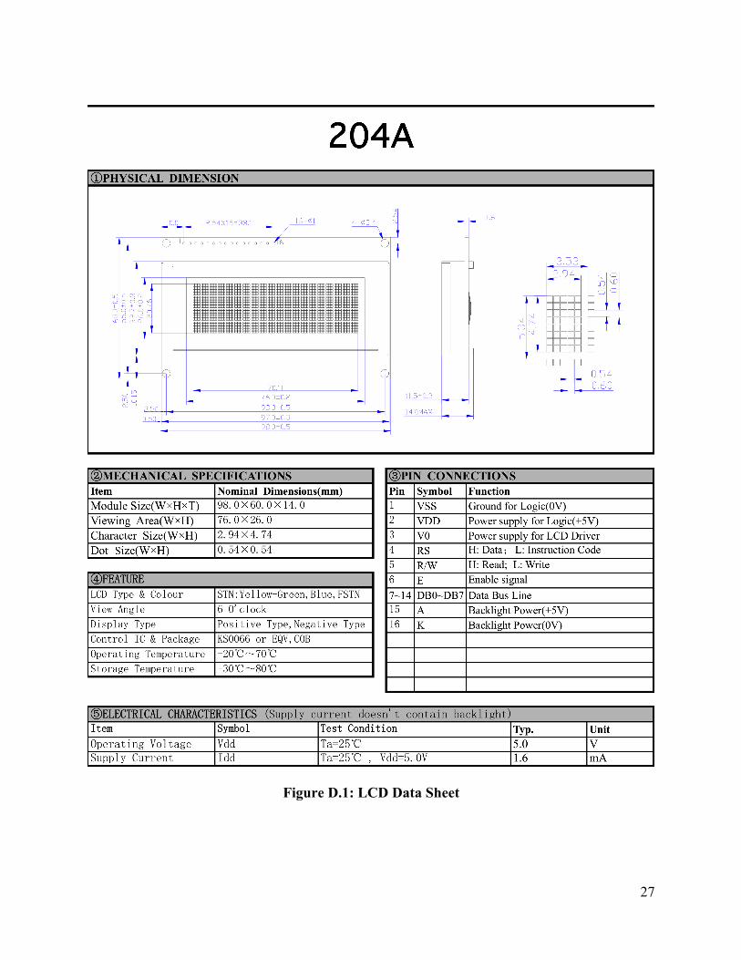
27
Figure D.1: LCD Data Sheet

28
Figure D.2: I2C Connector for LCD

29
Figure D.3: Keypad Data Sheet
Date Rev. Description
GOLDSUN ELECTRONICS CO., LTD.
UNIT: SCALE: CAS No:ERN No:SHEET 1 OF 1
DCC. NO.
A4 DRAWING NO.mm
Rev.Description1
DRAWN:
MATERIAL
Ivan Wang
VERIFY PEOPLE:
169245
JAMECO NO. GOLDSUN NO.
TELEPHONE 4x4 KEYPADSBLACK COLORPenny
AK-1607-N-BBW

30
Figure D.4: AD595 Data Sheet

31
Figure D.5: Servo Data Sheet

The Automated Personal Trainer: Intelligent Gym Equipment
The Pennsylvania State University: ME 445
Eric Steinour Vinny Pesce
May 3, 2013

Introduction
The objective of our project is to design intelligent gym equipment to serve as an electronic personal trainer for anyone who is trying to meet their fitness goals. Specifically, we focused on gym equipment and integrating electromechanical components into the equipment so that the user would easily be able to record and track their workout progress on each machine that they used. The two different areas of gym equipment that the team dedicated their time to were weight stack machines and free weights. We first brainstormed what the most efficient designs would be in order to accomplish the task on hand. We drew the circuits and tested these ideas in the lab using the breadboard. Once we had a solid understanding of what worked and what we were going to include on our actual prototype, we began transferring all of the components to the physical prototype. Motivation Both members of the team enjoy exercising regularly. When the team is exercising at fitness centers they frequently experience a pain point within the physical fitness equipment industry when they try to remember the amount of sets, weight, and repetitions they have done in the past in order to determine the correct number of sets, weight, and repetitions for their current workout on any given exercise. Many people walk around fitness centers with a notebook and a pencil to document their workout and to track their progress. However, the team searched for an innovative solution to this problem, and this is where the inspiration came for the project. This is a unique project with regards to the potential for the idea and the prototype developed as a result of the project to evolve into an actual product that can be used by novice gym enthusiasts around the world to record their workout results and track their progress. This has become extra motivation and incentive for the team. Industrial Design Industrial design was important on this product so that the interface was easy for any novice exerciser to understand and use. It is intended that operation of this equipment be nearly effortless, as the main focus of the user should be on their workout. The team also wanted to design the hardware for the weight stack machine as similar to a real weight stack machine as possible so that the team could realistically design the wiring and electronic components in the most reliable and efficient way. This could ensure that the performance of the weight stack machine was not sacrificed. Figure 1.1 below illustrates the most recent design. The free weight system can be imbedded in any piece of free weight equipment such as dumbbells, barbells, and plates.

Figure 1 - Sample User Experience: Weight Stack Prototype The major components within the weight stack machine are an IR LED, a photo-transistor, a circuit with resistors in series, a pushbutton with a pull-down transistor, a matrix type keypad, a Sparkfun 125 kHz RFID module connected to an USB reader, and an Arduino Uno. The Arduino acts as the command center within the system and reads all of the data entering the pins within it. The only time the Arduino writes to the system is when the RFID module needs reset by transmitting a LOW signal. The major components within the free weight system were an Arduino Fio, a 3.7 V Lithium polymer (LiPo) battery pack, two xBee wireless RF modules, a Parallax xBee USB shield, and an ADXL 335 three-axis accelerometer. The circuit diagrams and schematics can be found in Appendix 1.

The resistors in series are imbedded in the center bar that runs through the entire weight stack, as see in Figure 2 below. There are as many resistors as there are plates, and current is constantly running through the circuit. The voltage drop across each resistor is programmed into the Arduino to determine which weight is being used. To register this weight, we simply measure the total voltage drop across the resistors via the pin, which feeds directly into an analog input in the Arduino. For example, if we have five 1 k Ω resistors that each correspond to 10 pounds of weight, and we measure the voltage drop across two resistors, we know that the person is lifting 20 pounds of weight.
Figure 2 – Configuration of resistors (indicated with blue arrow) in series on central bar.
Place pin here to measure voltage
drop across the resistors above.

Weight Stack System Operation Traditionally, weight stacks work by placing the pin in the plate associated with their desired weight. This holds the plate onto the beam that runs through the entire stack, which is attached to a cable that runs to a bar or handle. To operate, the user pulls the bar which in turn raises the weight stack. The weight stack is operated by pulling the rope upward. An IR LED and a phototransistor are mounted to the vertical support of the machine and a piece of cardboard attached to the top plate passes through the two and “breaks” the beam coming through. The phototransistor recognizes this as a drop in voltage and counts that as half of a rep. One full rep is completed as the plate returns back to the initial position. There is a push button located just below the RFID scanner that is used to tell the system when a set has been completed.
Figure 3 – Weight stack prototype labeled.
RFID scanner
IR LED and
photo -
transistor
Pin to measure
voltage drop
Central beam

Since our project is intended to aid users in achieving fitness goals, it is extremely important that they get visual feedback from the machines. To simulate this experience, all of our equipment was designed to interact with either Arduino’s serial monitor or our computer’s serial terminal. Both pieces of equipment are initiated by the RFID scanner. Once a member scans their ID card, the software registers whether the member is previous user or new to that piece of equipment. If the gym member has previously used the equipment before, results from their most recent workout will be printed on the screen. Once they complete a set they must press the push button so the system knows that they have finished. The results are then printed to the serial monitor and the next set’s workout becomes available. This process is repeated for 4 total sets and then the workout summary is printed. We will now show the serial monitor as the user would be expected to see it. Step 1: Scan your card
Step 2: Recognized scanned card

Step 3: User performs first set after selecting the desired weight on the weight stack. Then the user presses the pushbutton to record the first set.
Step 4: The user continues with the remaining sets. Step 5: The final workout results are displayed after the final set is complete.

If they are using the equipment for the first time, we set up an example that allows the user to input information via a matrix keypad about their workout and select from one of three predetermined exercise plans- fat loss, muscle gain, or strength training. We then designed and programed the three workouts based off of typical workout plans you might find on a fitness website or in a fitness magazine. We illustrate the sequence of events printed in the serial terminal below: The program recognizes you as new to the machine. Prompts you to choose a workout. Suppose you want to strength train: You press # to continue The remainder of the program is executed as shown in the previous case where the user had exercised on that machine previously.
Hi! Please scan your card if you’re ready to sweat!
Please select a workout:
1: Fat loss
2: Muscle gain
3: Strength training
You have selected the STRENGTH TRAINING program. Here is
your workout:
4 sets, 8 reps per set
Press # to continue or press * to return to MAIN MENU
You are now using the STRENGTH TRAINING program.
Work hard and have fun! Remember to push the button
between sets.

Free Weight System Operation The idea of using an accelerometer to extend this project to free weights was developed late in the semester so it has not been incorporated into the program listed above. We have only been able to develop code to count the number of reps performed. In general, operation is very straightforward. The Arduino Fio, containing the accelerometer as shown below, was tested using a dumbbell curl motion.
Figure 4 – Arduino Fio with ADXL 335 accelerometer and xBee (not visible, located on
underside) To operate the Arduino was switched on, the xBee receiver (not shown) was connected to the computers serial port, and the serial monitor in Arduino was opened and the program counted the reps as they were completed. We found that the program worked well for standard curling, but if we tried to curl very slowly, the program was not always able to register it. This is due to the way we programmed the Arduino to read the accelerometer data.
Figure 5 – Raw data from accelerometer
1400
1500
1600
1700
1800
1900
2000
0 50 100 150 200 250 300
mV
/ g
Data point

Figure 4 shows the raw data being read from the accelerometer. The readings from the x-, y-, and z- axes were filtered using a moving average where we weighted the previous reading by 99.5% and the current reading by .5%. We found that the data wasn’t too noisy using this filter and that we could satisfactorily count reps at a standard pace. As this is a 3 axis accelerometer we chose to sum the absolute values of the readings from each axis to get a total. The sharp valleys correspond to each repetition, where the third valley around 125 was executed more slowly than the others. To register one rep we simply set a threshold for this reading so that if the current reading was 50 mV/g (background noise was at roughly 30-35 mV/g) more than the previous one, a rep should be counted. We then set a 1.5 second delay so as not to add any erroneous counts. We tried a number of filtering approaches and weighting values but found that this operation was best. It counted reps fairly well, except occasionally when the Arduino was moved slowly. A more robust program should be implemented to better deal with these variations. Configuring the xBees
Figure 6 – xBee and xBee shield for serial communication
The xBees must be configured before they can be used. Specifically, you must program them to have a specific ID, be able to recognize the ID of the other xBee, and have the same personal access network (PAN) ID, similar to setting two wireless radios to the same frequency, so that they can communicate with each other. We used a terminal program called PuTTY. Issues Much of the hardware for the weight stack worked as intended. However, it is not very robust for use in varied workouts. Some workouts require the plate to move only through a limited range, so it is possible that it doesn’t pass the IR sensor and phototransistor. This could potentially be designed for by using multiple sensors placed at different points along the weight stack. The free weight system was entirely monitored via the 3 axis accelerometer. To better count reps when the user is moving slow we should employ a better peak counting program. We

considered using higher order filtering techniques to smooth out the data but we were sampling data at .1 seconds so more advanced filtering would wash out the peaks. We chose .1 seconds because if we were almost continuously sampling the serial monitor couldn’t always accurate print out the values, which we used to generate graphs like Figure 4 to better gauge how we could modified our code to make counting more accurate. Future work Considering this project from a user view point, there is significant room for additional design. We feel that most of the hardware from our project would be sufficient for implementation in weight machines and free weights, so future work would heavily revolve around software development and industrial design, as we suggest that new equipment be designed to incorporate many of the components from our project. However, it is entirely possible to implement this hardware onto pre-existing equipment. Additionally, we feel that gym members should design a workout plan with a personal trainer and then have that workout plan be stored on a centralized computer. As the user visits each workout station, the relevant workout that has been designed for them will automatically register once they scan their ID card.

Appendix 1
Figure 7 – Wiring circuit for weight stack prototype. Green line represents pin.
Figure 8 – Circuit schematic for weight stack prototype.
Note: Matrix keypad not present as software did not have component. It has 8 pins, only 7 of which were used. See next figure for pin association.
Resistors attached to plate shaft
To K
eypad

Figure 9 – Matrix keypad with Arduino digital pin designations
Not used 12 11 10 9 8 7 6

Figure 10 – Wiring diagram for circuit imbedded in free weight equipment.
Figure 11 – Schematic of circuit imbedded in free weight equipment.
Figure 12 – xBee configuration on underside of Arduino Fio (xBee interface not available in schematic software).

Appendix 2 Arduino Code for Weight Stack //RFID char Eric[13]="4C0020EEAC2E"; //12 bit Hex code of RFID card 1 char Vinny[13]="4C0020D4E45C"; //12 bit Hex code of RFID card 2 int RFIDResetPin = 13; //digital write from TXR pin of RFID USB reader to reset RFID //Reps int reps = A1; int r=0; int reparray[10]; float count=0; int reparraypastEric[4]=9,9,9,9;//represent previous workout result of Eric int reparraypredictedEric[4]=8,8,8,8;//represent new workout data for Eric int reparraypastVinny[4]=0,0,0,0;//represent previous workout result of Vinny (none) int reparraypredictedVinny[4]=0,0,0,0;//represent new workout data for Vinny (none) //Weight int stack=A0; int w=0; int weightarray[10]; int weightarraypastEric[4]=30,30,25,25;//represent previous workout result of Eric int weightarraypredictedEric[4]=35,30,30,30; //represent new workout data for Eric int weightarraypastVinny[4]=0,0,0,0;//represent previous workout result of Vinny (none) int weightarraypredictedVinny[4]=0,0,0,0;//represent new workout data for Vinny (none) //Set int s=0; int setarray[10]; int resetbutton=2; int total_target_sets=4; int setarraypastEric[4]=1,2,3,4;//represent previous workout result of Eric int setarraypredictedEric[4]=1,2,3,4;//represent new workout data for Eric int setarraypastVinny[4]=0,0,0,0;//represent previous workout result of Vinny (none) int setarraypredictedVinny[4]=0,0,0,0;//represent new workout data for Vinny (none) // the setup routine runs once the code is uploaded: void setup() // initialize serial communication at 9600 bits per second: Serial.begin(9600); pinMode(stack, INPUT);

pinMode(reps,INPUT); pinMode(resetbutton, INPUT); Serial.println("Hi! Please scan your card if you're ready to sweat!"); void Read_RFID_card()//Reads correct 12 of 16 Hex characters within card code and places them in an array char tagString[13]; //initiate empty matrix tagString of 13 characters int index = 0; //set index to 0 boolean reading = false; //initiate reading to 0 while(Serial.available()) //while loop to run as long as 16 bytes are not used int readByte = Serial.read(); //read next available byte if(readByte == 2) reading = true; //begining of tag if(readByte == 3) reading = false; //end of tag if(reading && readByte != 2 && readByte != 10 && readByte != 13) //store tag in empty matrix tagString tagString[index] = readByte; index ++; //add one to index to run through next position in matrix the next time through the loop checkTag(tagString); //Check if it is a match // clearTag(tagString); //Clear the char of all value resetReader(); //reset the RFID reader void checkTag(char tag[])//check the read tag with known tags if(strlen(tag) == 0) return; //empty, no need to contunue if(compareTag(tag, Eric)) // if matched Eric, do this if (weightarraypastEric[0]!=0) Serial.println("Welcome back Eric!"); Serial.println("Previous Workout Results:"); Serial.print("Set");//print workout results from previous set Serial.print(" "); Serial.print("Weight"); Serial.print(" "); Serial.println("Reps"); Serial.print(setarraypastEric[0]); Serial.print(" "); Serial.print(weightarraypastEric[0]); Serial.print(" ");
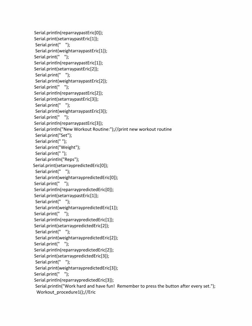
Serial.println(reparraypastEric[0]); Serial.print(setarraypastEric[1]); Serial.print(" "); Serial.print(weightarraypastEric[1]); Serial.print(" "); Serial.println(reparraypastEric[1]); Serial.print(setarraypastEric[2]); Serial.print(" "); Serial.print(weightarraypastEric[2]); Serial.print(" "); Serial.println(reparraypastEric[2]); Serial.print(setarraypastEric[3]); Serial.print(" "); Serial.print(weightarraypastEric[3]); Serial.print(" "); Serial.println(reparraypastEric[3]); Serial.println("New Workout Routine:");//print new workout routine Serial.print("Set"); Serial.print(" "); Serial.print("Weight"); Serial.print(" "); Serial.println("Reps"); Serial.print(setarraypredictedEric[0]); Serial.print(" "); Serial.print(weightarraypredictedEric[0]); Serial.print(" "); Serial.println(reparraypredictedEric[0]); Serial.print(setarraypastEric[1]); Serial.print(" "); Serial.print(weightarraypredictedEric[1]); Serial.print(" "); Serial.println(reparraypredictedEric[1]); Serial.print(setarraypredictedEric[2]); Serial.print(" "); Serial.print(weightarraypredictedEric[2]); Serial.print(" "); Serial.println(reparraypredictedEric[2]); Serial.print(setarraypredictedEric[3]); Serial.print(" "); Serial.print(weightarraypredictedEric[3]); Serial.print(" "); Serial.println(reparraypredictedEric[3]); Serial.println("Work hard and have fun! Remember to press the button after every set."); Workout_procedure1();//Eric

final_data_return(); else Serial.println("Eric, thanks for joning our team! Please see a personal trainer at the front desk to help with set-up."); else if(compareTag(tag, Vinny)) //if matched Vinny, do this if (weightarraypastVinny[0]!=0) Serial.println("Welcome back Vinny!"); Serial.println("Previous Workout Results:");//print workout results from previous set Serial.print("Set"); Serial.print(" "); Serial.print("Weight"); Serial.print(" "); Serial.println("Reps"); Serial.print(setarraypastVinny[0]); Serial.print(" "); Serial.print(weightarraypastVinny[0]); Serial.print(" "); Serial.println(reparraypastVinny[0]); Serial.print(setarraypastVinny[1]); Serial.print(" "); Serial.print(weightarraypastVinny[1]); Serial.print(" "); Serial.println(reparraypastVinny[1]); Serial.print(setarraypastVinny[2]); Serial.print(" "); Serial.print(weightarraypastVinny[2]); Serial.print(" "); Serial.println(reparraypastVinny[2]); Serial.print(setarraypastVinny[3]); Serial.print(" "); Serial.print(weightarraypastVinny[3]); Serial.print(" "); Serial.println(reparraypastVinny[3]); Serial.println("New Workout Routine:");//print new workout routine Serial.print("Set"); Serial.print(" "); Serial.print("Weight"); Serial.print(" "); Serial.println("Reps");

Serial.print(setarraypredictedVinny[0]); Serial.print(" "); Serial.print(weightarraypredictedVinny[0]); Serial.print(" "); Serial.println(reparraypredictedVinny[0]); Serial.print(setarraypastVinny[1]); Serial.print(" "); Serial.print(weightarraypredictedVinny[1]); Serial.print(" "); Serial.println(reparraypredictedVinny[1]); Serial.print(setarraypredictedVinny[2]); Serial.print(" "); Serial.print(weightarraypredictedVinny[2]); Serial.print(" "); Serial.println(reparraypredictedVinny[2]); Serial.print(setarraypredictedVinny[3]); Serial.print(" "); Serial.print(weightarraypredictedVinny[3]); Serial.print(" "); Serial.println(reparraypredictedVinny[3]); Serial.println("Work hard and have fun! Remember to press the button after every set."); Workout_procedure2();//Vinny final_data_return(); else Serial.println("Vinny, thanks for joning our team! Please see a personal trainer at the front desk to help with set-up."); boolean compareTag(char one[], char two[]) if(strlen(one) == 0) return false; //empty for(int i = 0; i < 12; i++) if(one[i] != two[i]) return false; //check all 12 bytes of input array and given array. return true; //no mismatches void resetReader() //Reset the RFID reader to read again. digitalWrite(RFIDResetPin, LOW);//write voltage to pin 13 at 0V digitalWrite(RFIDResetPin, HIGH);//write voltage to pin 13 at 5V

delay(150); void clearTag(char one[])//clear the char array by filling with null - ASCII 0 Will think same tag has been read otherwise for(int i = 0; i < strlen(one); i++) one[i] = 0; void rep_record()//function uses an if loop to count reps and place in an array if(analogRead(reps)>=1020) count=count+0.5; reparray[r]=count; delay(250); void weight_record() //function uses if and else if statements to record weight and place in an array float voltage = analogRead(stack) * (5.0 / 1023.0); //map voltage if (voltage>=4.95 and voltage<=5.05)//assign weight dependent upon voltage levels weightarray[w]=10; else if (voltage>=3.7 and voltage<=3.8) weightarray[w]=20; else if (voltage>=2.45 and voltage<=2.55) weightarray[w]=30; else if (voltage>=1.2 and voltage<=1.3) weightarray[w]=40; else if (voltage>=0 and voltage<=0.05) weightarray[w]=50; else weightarray[w]=0; void set() //function that calls on weight_record() and rep_record ()to run

count=0; int buttonState=digitalRead(resetbutton); while (buttonState==LOW) //loop only runs while pushbutton is left unarmed. weight_record(); rep_record(); setarray[s]=s+1; buttonState=digitalRead(resetbutton); void final_data_return()//spits out final data for workout just finished s=0; while (s==0) Serial.println("Great work today! Final Results:"); Serial.print("Set"); Serial.print(" "); Serial.print("Weight"); Serial.print(" "); Serial.println("Reps"); s++; s=0; while((s+1) <= total_target_sets) Serial.print(setarray[s]); Serial.print(" "); Serial.print(weightarray[s]); Serial.print(" "); Serial.println(reparray[s]); s++; void Workout_procedure1()//prints previous workout results and next sets suggested workout routine for Eric while ((s+1)<=total_target_sets) // the while loop routine runs until the current set plus one (s+1) is equal to the total target sets set(); //run set() function Serial.println("Actual Performance:"); Serial.print("Set");

Serial.print(" "); Serial.print("Weight"); Serial.print(" "); Serial.println("Reps"); Serial.print(setarray[s]); Serial.print(" "); Serial.print(weightarray[s]); Serial.print(" "); Serial.println(reparray[s]); if (s+1<total_target_sets) Serial.println("Good work! Below you will find your suggested weight and number of repititions for your next set."); Serial.println("Next Set's Weight and Reps"); Serial.print("Set"); Serial.print(" "); Serial.print("Weight"); Serial.print(" "); Serial.println("Reps"); Serial.print(setarraypredictedEric[s+1]); Serial.print(" "); Serial.print(weightarraypredictedEric[s+1]); Serial.print(" "); Serial.println(reparraypredictedEric[s+1]); delay(1000); s++; //add one to s each time through the loop w++; //add one to w each time through the loop r++;//add one to r each time through the loop void Workout_procedure2()//prints previous workout results and next sets suggested workout routine for Vinny while ((s+1)<=total_target_sets) // the while loop routine runs until the current set plus one (s+1) is equal to the total target sets set(); //run set() function Serial.println("Actual Performance:"); Serial.print("Set"); Serial.print(" "); Serial.print("Weight"); Serial.print(" "); Serial.println("Reps");

Serial.print(setarray[s]); Serial.print(" "); Serial.print(weightarray[s]); Serial.print(" "); Serial.println(reparray[s]); if (s+1<total_target_sets) Serial.println("Good work! Below you will find your suggested weight and number of repititions for your next set."); Serial.println("Next Set's Weight and Reps"); Serial.print("Set"); Serial.print(" "); Serial.print("Weight"); Serial.print(" "); Serial.println("Reps"); Serial.print(setarraypredictedVinny[s+1]); Serial.print(" "); Serial.print(weightarraypredictedVinny[s+1]); Serial.print(" "); Serial.println(reparraypredictedVinny[s+1]); delay(1000); s++; //add one to s each time through the loop w++; //add one to w each time through the loop r++;//add one to r each time through the loop //loop runs constantly to read a card that is scanned at anytime void loop() Read_RFID_card(); //reads RFID card

Appendix 3 Arduino Code for New User /* Keypadtest.pde * * Demonstrate the simplest use of the keypad library. * * The first step is to connect your keypad to the * Arduino using the pin numbers listed below in * rowPins[] and colPins[]. If you want to use different * pins then you can change the numbers below to * match your setup. * * Code modified from website: http://playground.arduino.cc/code/Keypad */ #include <Keypad.h> const byte ROWS = 4; // Four rows const byte COLS = 3; // Three columns // Define the Keymap char keys[ROWS][COLS] = '1','2','3', '4','5','6', '7','8','9', '#','0','*' ; // Connect keypad ROW0, ROW1, ROW2 and ROW3 to these Arduino pins. byte rowPins[ROWS] = 9, 8, 7, 6 ; // Connect keypad COL0, COL1 and COL2 to these Arduino pins. byte colPins[COLS] = 12, 11, 10 ; // Create the Keypad Keypad kpd = Keypad( makeKeymap(keys), rowPins, colPins, ROWS, COLS ); // Function to clear Serial terminal (Terminal program for Mac) // void clearAndHome() Serial.write(27); // ESC Serial.print("[2J"); // clear screen Serial.write(27); // ESC

Serial.print("[H"); // cursor to home void setup() clearAndHome(); Serial.print("Please select a workout:"); Serial.println(); Serial.print("1: Fat loss"); Serial.println(); Serial.print("2: Mass gain"); Serial.println(); Serial.print("3: Strength training"); Serial.println(); void loop() char key = kpd.getKey(); if(key) // Check for a valid key. switch (key) case '1': clearAndHome(); Serial.print("You have selected the FAT LOSS program."); Serial.println(); delay(500); Serial.print("Here is your workout:"); Serial.println(); delay(500); Serial.print("3 sets, 12 reps per set"); Serial.println(); Serial.println(); delay(1000); Serial.print("Press # to continue or * to return to main menu"); break; case '2': clearAndHome(); //Serial.clear(); Serial.print("You have selected the MASS GAIN program."); Serial.println(); delay(500);
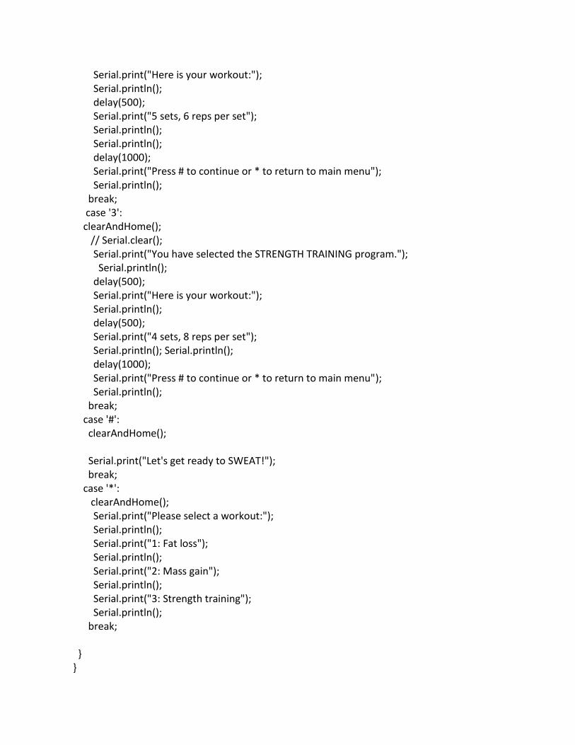
Serial.print("Here is your workout:"); Serial.println(); delay(500); Serial.print("5 sets, 6 reps per set"); Serial.println(); Serial.println(); delay(1000); Serial.print("Press # to continue or * to return to main menu"); Serial.println(); break; case '3': clearAndHome(); // Serial.clear(); Serial.print("You have selected the STRENGTH TRAINING program."); Serial.println(); delay(500); Serial.print("Here is your workout:"); Serial.println(); delay(500); Serial.print("4 sets, 8 reps per set"); Serial.println(); Serial.println(); delay(1000); Serial.print("Press # to continue or * to return to main menu"); Serial.println(); break; case '#': clearAndHome(); Serial.print("Let's get ready to SWEAT!"); break; case '*': clearAndHome(); Serial.print("Please select a workout:"); Serial.println(); Serial.print("1: Fat loss"); Serial.println(); Serial.print("2: Mass gain"); Serial.println(); Serial.print("3: Strength training"); Serial.println(); break;
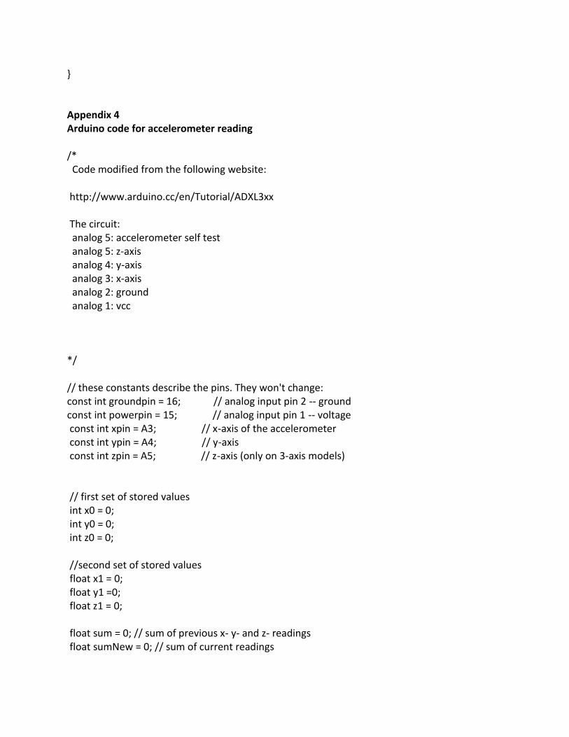
Appendix 4 Arduino code for accelerometer reading /* Code modified from the following website: http://www.arduino.cc/en/Tutorial/ADXL3xx The circuit: analog 5: accelerometer self test analog 5: z-axis analog 4: y-axis analog 3: x-axis analog 2: ground analog 1: vcc */ // these constants describe the pins. They won't change: const int groundpin = 16; // analog input pin 2 -- ground const int powerpin = 15; // analog input pin 1 -- voltage const int xpin = A3; // x-axis of the accelerometer const int ypin = A4; // y-axis const int zpin = A5; // z-axis (only on 3-axis models) // first set of stored values int x0 = 0; int y0 = 0; int z0 = 0; //second set of stored values float x1 = 0; float y1 =0; float z1 = 0; float sum = 0; // sum of previous x- y- and z- readings float sumNew = 0; // sum of current readings

float w = 0.995; // weighting function for previous time step data int count = 0; // total reps completed void setup() // initialize the serial communications: Serial.begin(9600); delay(5000); // Provide ground and power by using the analog inputs as normal // digital pins. This makes it possible to directly connect the // breakout board to the Arduino. If you use the normal 5V and // GND pins on the Arduino, you can remove these lines. pinMode(groundpin, OUTPUT); pinMode(powerpin, OUTPUT); digitalWrite(groundpin, LOW); digitalWrite(powerpin, HIGH); void loop() // get initial readings x0 = analogRead(xpin); y0 = analogRead(ypin); z0 = analogRead(zpin); delay(100); //Smoothing out the data using previous reading x1 = w*x0 + (1-w)*analogRead(xpin); y1 = w*y0 + (1-w)*analogRead(ypin); z1 = w*z0 + (1-w)*analogRead(zpin); sumNew = abs(x1)+abs(y1)+abs(z1); if ((sumNew-sum)>55) // compare diffenrece against a threshold count++; Serial.print(count); Serial.println(); delay (1500);


Modernization of a Planar Near-Field
Measurement System for Use with
Modern Technology
Alex Punzi and Edgar Yip
ME 445: Microcomputer Interfacing
Prepared for: Dr. Henry J. Sommer III and Mike Robinson
May 2, 2013

i
Acknowledgements
We would like to thank to Dr. Sommer for his guidance and teaching the material necessary to make this
project possible. We would also like Dr. Erik Lenzing of the Penn State Applied Research Lab for funding
this project and all of his help. Finally, we would like to thank Mike Robinson for all of his time and help
with evaluating the hardware and the Arduino code.
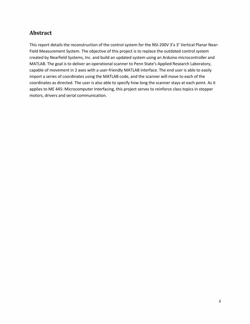
ii
Abstract
This report details the reconstruction of the control system for the NSI-200V 3’x 3’ Vertical Planar Near-
Field Measurement System. The objective of this project is to replace the outdated control system
created by Nearfield Systems, Inc. and build an updated system using an Arduino microcontroller and
MATLAB. The goal is to deliver an operational scanner to Penn State’s Applied Research Laboratory,
capable of movement in 2 axes with a user-friendly MATLAB interface. The end user is able to easily
import a series of coordinates using the MATLAB code, and the scanner will move to each of the
coordinates as directed. The user is also able to specify how long the scanner stays at each point. As it
applies to ME 445: Microcomputer Interfacing, this project serves to reinforce class topics in stepper
motors, drivers and serial communication.

iii
Table of Contents Acknowledgements ........................................................................................................................................ i
Abstract ......................................................................................................................................................... ii
1.0 Introduction ............................................................................................................................................ 1
2.0 Examination of Antenna Range Controller Components ........................................................................ 4
3.0 Adaptation using Arduino Uno ............................................................................................................... 7
3.1 Motor Noise Issues ............................................................................................................................. 9
4.0 Specifying Coordinates for a Scan ......................................................................................................... 11
4.1 Importing and Checking the Data File ............................................................................................... 12
5.0 Serial Communication ........................................................................................................................... 13
5.1 Establishing Serial Communication in Arduino ................................................................................. 13
5.2 Establishing Serial Communication in MATLAB ................................................................................ 14
5.3 Exchanging Serial Data between MATLAB and Arduino ................................................................... 14
6.0 Moving to Assigned Coordinates .......................................................................................................... 16
6.1 Setting to Home ................................................................................................................................ 16
6.2 Moving the scanner .......................................................................................................................... 16
6.3 Reading the Emergency Stops .......................................................................................................... 18
6.4 Clearing the Serial Port ..................................................................................................................... 18
7.0 Conclusions ........................................................................................................................................... 18
Appendix A – Motor Driver Specifications .................................................................................................. 20
Appendix B – End Stop Data Sheet ............................................................................................................. 21
Appendix C – Interpolation Examples ......................................................................................................... 23
Appendix D –MATLAB Code ........................................................................................................................ 24
Appendix E – Arduino Code ........................................................................................................................ 26
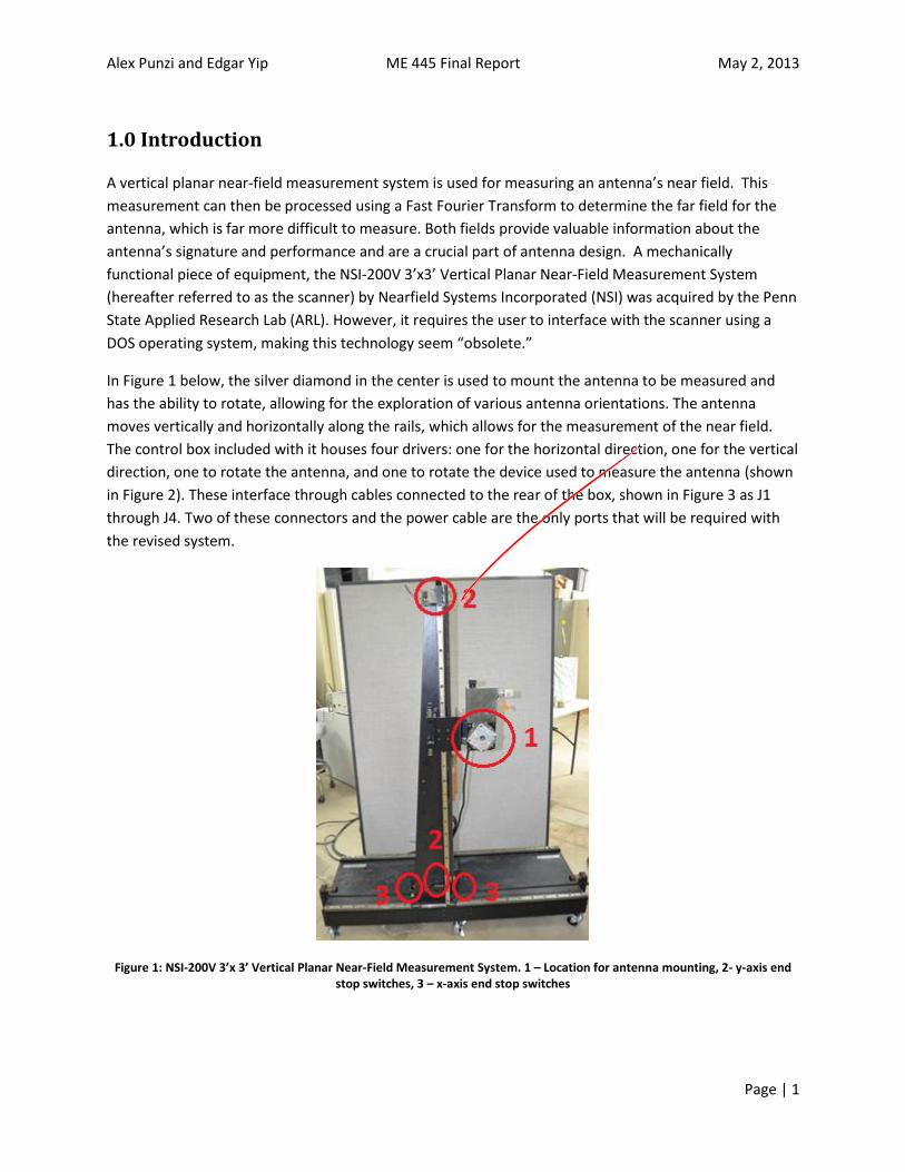
Alex Punzi and Edgar Yip ME 445 Final Report May 2, 2013
Page | 1
1.0 Introduction
A vertical planar near-field measurement system is used for measuring an antenna’s near field. This
measurement can then be processed using a Fast Fourier Transform to determine the far field for the
antenna, which is far more difficult to measure. Both fields provide valuable information about the
antenna’s signature and performance and are a crucial part of antenna design. A mechanically
functional piece of equipment, the NSI-200V 3’x3’ Vertical Planar Near-Field Measurement System
(hereafter referred to as the scanner) by Nearfield Systems Incorporated (NSI) was acquired by the Penn
State Applied Research Lab (ARL). However, it requires the user to interface with the scanner using a
DOS operating system, making this technology seem “obsolete.”
In Figure 1 below, the silver diamond in the center is used to mount the antenna to be measured and
has the ability to rotate, allowing for the exploration of various antenna orientations. The antenna
moves vertically and horizontally along the rails, which allows for the measurement of the near field.
The control box included with it houses four drivers: one for the horizontal direction, one for the vertical
direction, one to rotate the antenna, and one to rotate the device used to measure the antenna (shown
in Figure 2). These interface through cables connected to the rear of the box, shown in Figure 3 as J1
through J4. Two of these connectors and the power cable are the only ports that will be required with
the revised system.
Figure 1: NSI-200V 3’x 3’ Vertical Planar Near-Field Measurement System. 1 – Location for antenna mounting, 2- y-axis end stop switches, 3 – x-axis end stop switches

Alex Punzi and Edgar Yip ME 445 Final Report May 2, 2013
Page | 2
Figure 2: Mount for antenna measurement device, which is external to scanner system.
Figure 3: Rear of Antenna Range Controller, which contains connections for motors. On the left are the serial connectors used with the previous system.

Alex Punzi and Edgar Yip ME 445 Final Report May 2, 2013
Page | 3
The goal of the project is to circumvent the existing DOS interface and control the scanner using a serial
port (USB) connection and software in a Windows 7 environment. To accomplish this goal, the driver
connections, which previously interfaced with the software through a DB37 connector, and end stops
need to be analyzed and reconfigured. To do this, the current pinout of the system is determined. The
connections are then re-pinned to the proper locations. An Arduino is used to control the scanner
motors. The Arduino code takes an input from MATLAB code, which prompts the user for an array of
position data to be sent to the Arduino via its serial connection.

Alex Punzi and Edgar Yip ME 445 Final Report May 2, 2013
Page | 4
2.0 Examination of Antenna Range Controller Components
The first step in this project was to open NSI’s controller box and determine which components are
necessary for operation and what components, if any, would need to be replaced. Figure 4 shows the
inner components of the Antenna Range Controller (ARC), the hardware interface for the scanner.
Figure 4: NSI ARC. 1 - NSI Proprietary Control Board, 2 - Motor Drivers, 3 - Step Down Transformers, 4 - Fuse
By examining these components it is clear that the printed circuit board in the back corner of the case is
the control board used to operate the motor drivers. There are two transformers in the box which step
down the wall supply voltage from 120 VAC to 2 VAC and 30 VAC used to power the motor drivers. The
four motor drivers are all Anaheim Automation BLD72-1 Bilevel Step Motor Drivers. The technical
specifications for the drivers can be found in Appendix A. Table 1 describes the terminal block
connections on the motor drivers.
Table 1: BLD72-1 terminal block connections
Terminal # Description
1 Motor, Phase 1
2 Motor, Phase 3
3 Motor, Common 1, 3
4 Fault Reset
5 Direction (CCW)
6 Clock (CW)
7 0V DC
8 Half-Step/Full-Step
9 On/Off
10 N/C
11 Motor, Common 2, 4
12 Motor, Phase 2
13 Motor, Phase 4
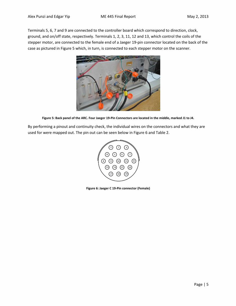
Alex Punzi and Edgar Yip ME 445 Final Report May 2, 2013
Page | 5
Terminals 5, 6, 7 and 9 are connected to the controller board which correspond to direction, clock,
ground, and on/off state, respectively. Terminals 1, 2, 3, 11, 12 and 13, which control the coils of the
stepper motor, are connected to the female end of a Jaeger 19-pin connector located on the back of the
case as pictured in Figure 5 which, in turn, is connected to each stepper motor on the scanner.
Figure 5: Back panel of the ARC. Four Jaeger 19-Pin Connectors are located in the middle, marked J1 to J4.
By performing a pinout and continuity check, the individual wires on the connectors and what they are
used for were mapped out. The pin out can be seen below in Figure 6 and Table 2.
Figure 6: Jaeger C 19-Pin connector (Female)
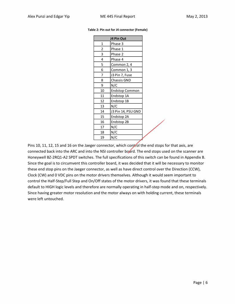
Alex Punzi and Edgar Yip ME 445 Final Report May 2, 2013
Page | 6
Table 2: Pin out for J4 connector (Female)
Pins 10, 11, 12, 15 and 16 on the Jaeger connector, which control the end stops for that axis, are
connected back into the ARC and into the NSI controller board. The end stops used on the scanner are
Honeywell BZ-2RQ1-A2 SPDT switches. The full specifications of this switch can be found in Appendix B.
Since the goal is to circumvent this controller board, it was decided that it will be necessary to monitor
these end stop pins on the Jaeger connector, as well as have direct control over the Direction (CCW),
Clock (CW) and 0 VDC pins on the motor drivers themselves. Although it would seem important to
control the Half-Step/Full Step and On/Off states of the motor drivers, it was found that these terminals
default to HIGH logic levels and therefore are normally operating in half-step mode and on, respectively.
Since having greater motor resolution and the motor always on with holding current, these terminals
were left untouched.
1 Phase 3
2 Phase 1
3 Phase 2
4 Phase 4
5 Common 2, 4
6 Common 1, 3
7 J3 Pin 7, Fuse
8 Chassis GND
9 N/C
10 Endstop Common
11 Endstop 1A
12 Endstop 1B
13 N/C
14 J3 Pin 14, PSU GND
15 Endstop 2A
16 Endstop 2B
17 N/C
18 N/C
19 N/C
J4 Pin Out

Alex Punzi and Edgar Yip ME 445 Final Report May 2, 2013
Page | 7
3.0 Adaptation using Arduino Uno
The end goal of the project involves operation of the x- and y-axes of the scanner. Because of this,
control of two of the four motor drivers within the ARC as well as the end stops associated with those
axes is the scope of this project. After this aspect is successfully completed, the other two axes can be
incorporated using similar methods. However, the rotational axes do not have end stops, which would
be needed to prevent harmfully twisting the wires of the mounted object. Controlling the other two
axes will be part of the next phase of the project, to be completed by two young engineering students
this summer. The Arduino Uno will be a suitable microcontroller for this application because of its ease
of use and sufficient pin availability. The bill of materials for this project is detailed in Table 7.The full
circuit diagram for the Arduino setup can be found in Figure 8.
Table 7: Bill of materials
Item Description Part No. Vendor Qty. Cost
Arduino UNO REV3 276-128 Radioshack 1 $29.99
1 μF Capacitor 272-996 Radioshack 1 $1.49
560 Ω Resistor 271-1116 Radioshack 1 $1.49
1.5 kΩ Resistor 271-1120 Radioshack 1 $1.49
Printed Circuit Board 276-170 Radioshack 1 $3.49
$37.95TOTAL
Bill of Materials
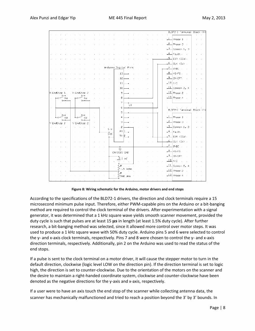
Alex Punzi and Edgar Yip ME 445 Final Report May 2, 2013
Page | 8
Figure 8: Wiring schematic for the Arduino, motor drivers and end stops
According to the specifications of the BLD72-1 drivers, the direction and clock terminals require a 15 microsecond minimum pulse input. Therefore, either PWM-capable pins on the Arduino or a bit-banging method are required to control the clock terminal of the drivers. After experimentation with a signal generator, it was determined that a 1 kHz square wave yields smooth scanner movement, provided the duty cycle is such that pulses are at least 15 in length (at least 1.5% duty cycle). After further research, a bit-banging method was selected, since it allowed more control over motor steps. It was used to produce a 1 kHz square wave with 50% duty cycle. Arduino pins 5 and 6 were selected to control the y- and x-axis clock terminals, respectively. Pins 7 and 8 were chosen to control the y- and x-axis direction terminals, respectively. Additionally, pin 2 on the Arduino was used to read the status of the end stops.
If a pulse is sent to the clock terminal on a motor driver, it will cause the stepper motor to turn in the default direction, clockwise (logic level LOW on the direction pin). If the direction terminal is set to logic high, the direction is set to counter-clockwise. Due to the orientation of the motors on the scanner and the desire to maintain a right-handed coordinate system, clockwise and counter-clockwise have been denoted as the negative directions for the y-axis and x-axis, respectively.
If a user were to have an axis touch the end stop of the scanner while collecting antenna data, the
scanner has mechanically malfunctioned and tried to reach a position beyond the 3’ by 3’ bounds. In

Alex Punzi and Edgar Yip ME 445 Final Report May 2, 2013
Page | 9
order to prevent such a situation in which the scanner can be damaged, it was decided to use the end
stop switches as emergency stops. In addition to being used to initially zero the x- and y-positions of the
scanner, the end stops will automatically terminate all movement on the scanner if activated. This is
done by using the switches from single-pole, double-throw to single-pole, single-throw. The Arduino
supplies 5 V to each of the common poles on all four end stops. The normally open terminal on every
end stop is then fed into pin 2 on the Arduino (after being filtered, as discussed in the next section),
where it is pulled down to 0 V. This allows the status of all the end stops to be read at once. If any of the
end stops are triggered, pin 2 will be read as logic HIGH, terminate the process currently running, and
halt the scanner.
During testing, it was discovered that the stepper motors introduced noise issues in the end stop line
when operating. The noise issues were significant enough to falsely trigger the end stop reading as logic
level HIGH, resulting in premature stops. In order to have the end stops work as intended, a pull down
resistor and a passive first-order low pass filter were implemented to mitigate the noise.
3.1 Motor Noise Issues
In order to find out what was causing the end stop to falsely trigger, an oscilloscope was used to monitor
the incoming end stop signal to the Arduino. The end stop signal was pulled down to reduce the stress
on the Arduino to hold the pin high, as well as provide more margin to the next logic level (for Arduino,
3 V for LOW to HIGH, 2 V from HIGH to LOW). A 560 resistor was used for the pull down resistor. A
small resistance value was used to dissipate the energy from the noise pulses more quickly. Figure 9
shows the raw signal while the y-axis motor is in operation.
Figure 9: Y-axis end stop reading using a pull down resistor without common ground or a filter.
Although the signal hovers about 0 volts, large voltage spikes can be seen in the captured data. The
Arduino code is written such that all movement on the scanner is terminated if an end stop, at any
-0.02 -0.015 -0.01 -0.005 0 0.005 0.01 0.015 0.02-20
-10
0
10
20
30
40
50
60
70Y Endstop Reading without Common Ground or Low Pass Filter
Time (seconds)
Voltage (
V)

Alex Punzi and Edgar Yip ME 445 Final Report May 2, 2013
Page | 10
point, is read as logic level HIGH. This caused our motors to terminate prematurely before reaching their
destination. Because the signal is only erratic when a motor is running, it was concluded that it is motor
noise that is causing the end stop signal to trigger. Using twisted pair wires for the end stop connections
was attempted to solve the issue but was not successful.
The next step taken to mitigate the problem was to use a common ground between the Arduino and the
ARC. It was realized that the end stop circuitry was grounded via the Arduino and the motor drivers
were grounded via the ARC chassis, but they were not grounded to each other. This caused a voltage
potential between the two. By connecting the Arduino ground to the ARC chassis, a common ground
was established. Figure 10 shows the improved signal after introducing this common ground.
Figure 10: Y-axis end stop reading using a pull down resistor, a common ground, and no filter.
After the Arduino is grounded to the chassis, the signal exhibited significant improvement, but the end
stops still triggered. Although the amplitude of the voltage spikes had been reduced, the spikes still
carry enough energy to cause the end stops to accidentally trigger.
The next attempt to eliminate the noise was to introduce a passive, first-order, low-pass filter to the
signal to reduce this noise. Figures 9 and 10 show that the noise in our signal causes 39 voltage spikes
over the course of 0.04 seconds. The frequency of the noise can then be calculated as shown below:
A 1 µF capacitor and a 1.5 kΩ resistor in were selected for the filter. Using these components, a filter
with a cutoff frequency of 106 Hz is created, as calculated below.
-0.02 -0.015 -0.01 -0.005 0 0.005 0.01 0.015 0.02-20
-10
0
10
20
30
40
50Y Endstop Reading with Common Ground
Time (seconds)
Voltage (
V)
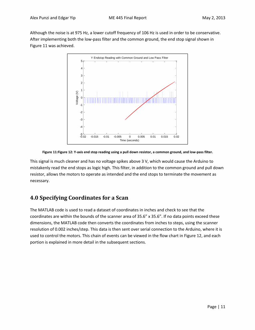
Alex Punzi and Edgar Yip ME 445 Final Report May 2, 2013
Page | 11
Although the noise is at 975 Hz, a lower cutoff frequency of 106 Hz is used in order to be conservative.
After implementing both the low-pass filter and the common ground, the end stop signal shown in
Figure 11 was achieved.
Figure 11:Figure 12: Y-axis end stop reading using a pull down resistor, a common ground, and low-pass filter.
This signal is much cleaner and has no voltage spikes above 3 V, which would cause the Arduino to
mistakenly read the end stops as logic high. This filter, in addition to the common ground and pull down
resistor, allows the motors to operate as intended and the end stops to terminate the movement as
necessary.
4.0 Specifying Coordinates for a Scan
The MATLAB code is used to read a dataset of coordinates in inches and check to see that the
coordinates are within the bounds of the scanner area of 35.6” x 35.6”. If no data points exceed these
dimensions, the MATLAB code then converts the coordinates from inches to steps, using the scanner
resolution of 0.002 inches/step. This data is then sent over serial connection to the Arduino, where it is
used to control the motors. This chain of events can be viewed in the flow chart in Figure 12, and each
portion is explained in more detail in the subsequent sections.
-0.02 -0.015 -0.01 -0.005 0 0.005 0.01 0.015 0.02-5
-4
-3
-2
-1
0
1
2
3
4
5Y Endstop Reading with Common Ground and Low Pass Filter
Time (seconds)
Voltage (
V)
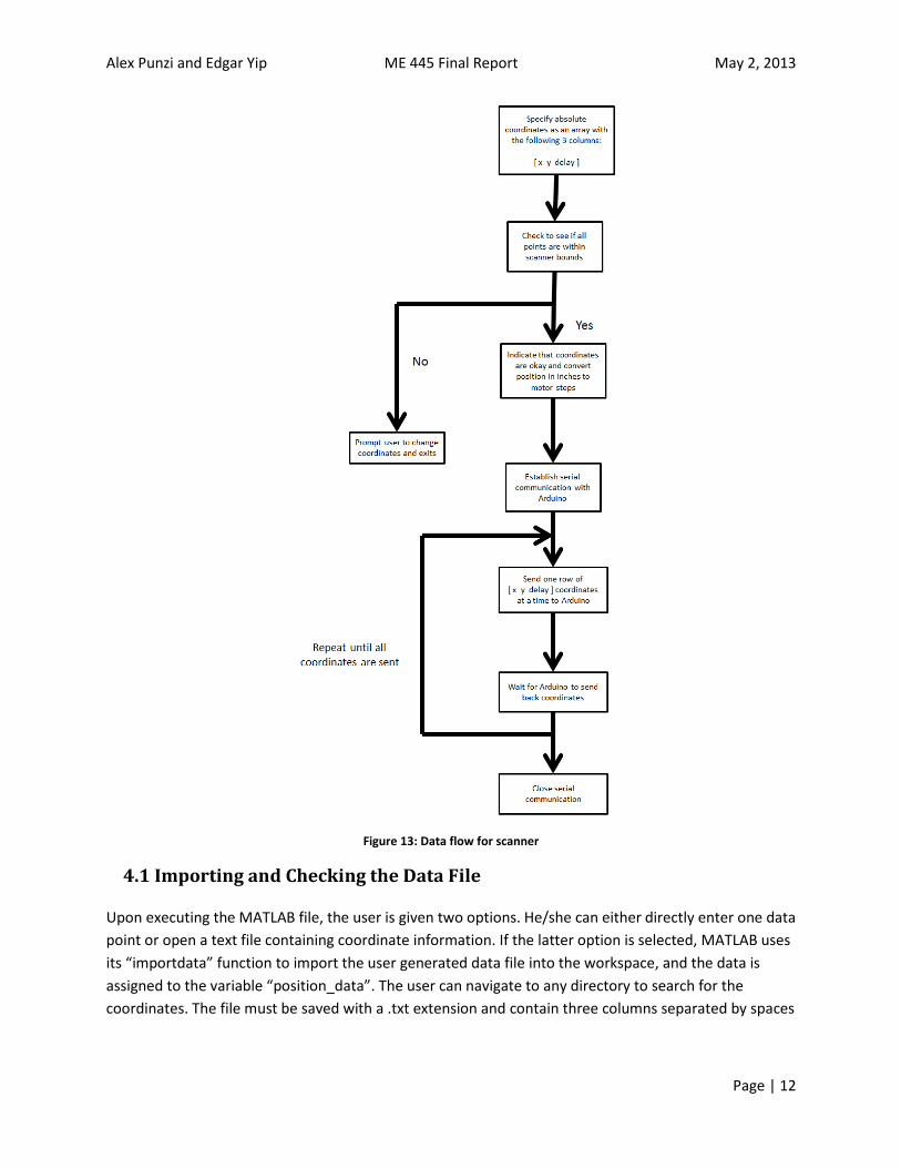
Alex Punzi and Edgar Yip ME 445 Final Report May 2, 2013
Page | 12
Figure 13: Data flow for scanner
4.1 Importing and Checking the Data File
Upon executing the MATLAB file, the user is given two options. He/she can either directly enter one data
point or open a text file containing coordinate information. If the latter option is selected, MATLAB uses
its “importdata” function to import the user generated data file into the workspace, and the data is
assigned to the variable “position_data”. The user can navigate to any directory to search for the
coordinates. The file must be saved with a .txt extension and contain three columns separated by spaces

Alex Punzi and Edgar Yip ME 445 Final Report May 2, 2013
Page | 13
corresponding to x-coordinates, y-coordinates (both in inches), and the desired delay in milliseconds at
each point. Each row corresponds to one data point.
Once the data is imported, it is checked against the scanner limits. It does this by finding the values that
are larger than these limits using MATLAB’s “find” function. If any values are found to exceed the
scanner limits, the user is told which values are problematic, where they can be found, and exits the m-
file. This portion of the code is given in Figure 13.
Figure 14: MATLAB code used to check coordinate data for problematic values that lie outside of scanner range.
5.0 Serial Communication
One of the requirements established by ARL for the project was the ability to read a set of coordinate
data in a given format for use by the scanner. It was preferred by the end users that this process be
performed by MATLAB, a language familiar to them. Additionally, this enables use of the scanner
without the need to learn the Arduino programming environment. This task was achieved by
establishing a serial connection between the Arduino and MATLAB. The serial connection with the same
data transfer (Baud) rate must be established by both programs, which was selected to be 9600 bit/s.
5.1 Establishing Serial Communication in Arduino
In the Arduino environment, all that is needed to open this serial line is the command
“Serial.begin(9600)”. After this command, it is good practice to set a brief timeout ( ms) for the
serial line using “Serial.setTimeout()”, then use the “Serial.flush()” command to clear any values already
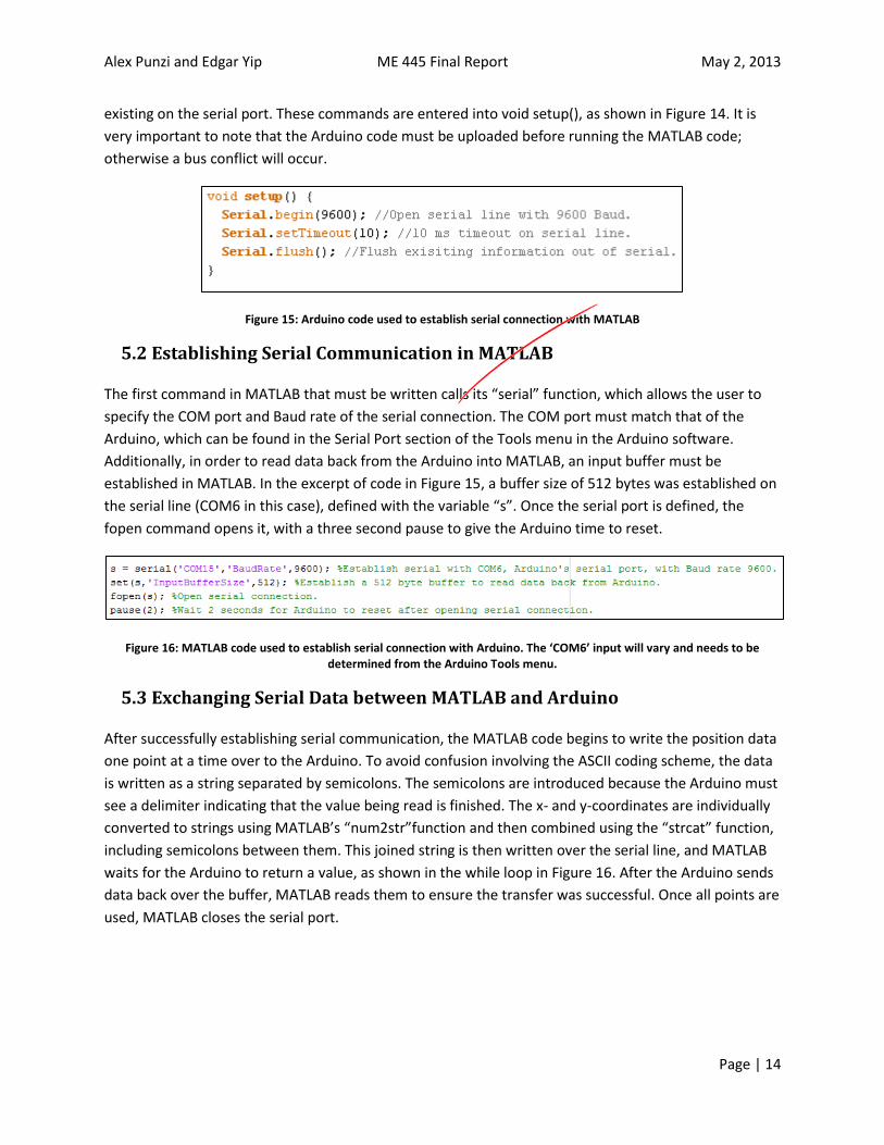
Alex Punzi and Edgar Yip ME 445 Final Report May 2, 2013
Page | 14
existing on the serial port. These commands are entered into void setup(), as shown in Figure 14. It is
very important to note that the Arduino code must be uploaded before running the MATLAB code;
otherwise a bus conflict will occur.
Figure 15: Arduino code used to establish serial connection with MATLAB
5.2 Establishing Serial Communication in MATLAB
The first command in MATLAB that must be written calls its “serial” function, which allows the user to
specify the COM port and Baud rate of the serial connection. The COM port must match that of the
Arduino, which can be found in the Serial Port section of the Tools menu in the Arduino software.
Additionally, in order to read data back from the Arduino into MATLAB, an input buffer must be
established in MATLAB. In the excerpt of code in Figure 15, a buffer size of 512 bytes was established on
the serial line (COM6 in this case), defined with the variable “s”. Once the serial port is defined, the
fopen command opens it, with a three second pause to give the Arduino time to reset.
Figure 16: MATLAB code used to establish serial connection with Arduino. The ‘COM6’ input will vary and needs to be determined from the Arduino Tools menu.
5.3 Exchanging Serial Data between MATLAB and Arduino
After successfully establishing serial communication, the MATLAB code begins to write the position data
one point at a time over to the Arduino. To avoid confusion involving the ASCII coding scheme, the data
is written as a string separated by semicolons. The semicolons are introduced because the Arduino must
see a delimiter indicating that the value being read is finished. The x- and y-coordinates are individually
converted to strings using MATLAB’s “num2str”function and then combined using the “strcat” function,
including semicolons between them. This joined string is then written over the serial line, and MATLAB
waits for the Arduino to return a value, as shown in the while loop in Figure 16. After the Arduino sends
data back over the buffer, MATLAB reads them to ensure the transfer was successful. Once all points are
used, MATLAB closes the serial port.

Alex Punzi and Edgar Yip ME 445 Final Report May 2, 2013
Page | 15
Figure 17: MATLAB code used to write coordinates over serial connection from MATLAB to Arduino.
Since the data sent by MATLAB provides step information, it will always be an integer value.
Consequently, Arduino’s “Serial.parseInt()” function is used to read in the data. This function was
selected after determining that serial communication between MATLAB and Arduino does not work well
using “Serial.read()” for integers larger than 8 bits (255 steps). Upon entering the primary loop, the
Arduino waits until bytes appear on the serial line. Once data appears (which will be multiple bytes
containing the first row of the position information), it stores the value before the first semicolon as
“StepsX”, the second value as “StepsY”, and the third value as “PauseBtwPoints”. The scanner is moved
to the desired position and then calls the “Serial_flush()” function to ensure no data remains on the line
and to hold the scanner at that point for the specified time. It then prints back a command to MATLAB
indicating successful data transfer. MATLAB will then send the next row of position information, if it
exists. The code used to read the data is given in Figure 17. The code used to clear the serial line, hold
the scanner, and send back a value to MATLAB indicating successful execution is given in Figure 18.
Figure 18: Arduino code used to read coordinates and delay from the serial connection.
Figure 19: Arduino code used to clear serial connection, hold the scanner, and print a value back to MATLAB indicating successful data import.

Alex Punzi and Edgar Yip ME 445 Final Report May 2, 2013
Page | 16
6.0 Moving to Assigned Coordinates
6.1 Setting to Home
Once the serial communication is established and the Arduino has received all the input data required
from the user, the scanner will first bring the antenna to the origin and zero the position. In order to do
this, the Arduino calls the function “SetToHome()”, which runs the motors in the negative direction one
axis at a time until their respective end stops are triggered. It does this using a while loop, as given in
Figure 19 for the x-direction. Once the end stop is triggered, the motors are halted and move 50 steps
into the positive direction. This is equivalent to 0.1 inch, achieved by switching the direction and setting
the clock pin high and low 50 times. This position is then set equal to zero.
Figure 20: Arduino code used to set the scanner to the home position (0.1 inches away from each endstop) in the bottom right corner.
6.2 Moving the scanner
The Arduino code moves the scanner using two separate functions. The first, “MoveXY”, determines
how many steps the motors need to take to reach the target position (relative to the current position). It
does this by accepting the target steps required in both directions as inputs. After checking if the target
x-position is positive or negative, linear interpolation is used to ensure the motors move in a straight line
to the target position. An integer ‘x’ is incremented by a constant value until it reaches the target
number of steps in the x-direction. This, with the coordinates of the target value, is used to dictate the
number of steps needed in the y-direction for each value of x. Since this y-value is continuously
increasing due to increasing ‘x’, it is subtracted from the last y-value to give the number of steps relative
to the last increment. A flow chart illustrating this process is given in Figure 20. A screenshot of the
function performing the interpolation, “linear_fit”, can be viewed in Figure 21.Example values for this
process can be viewed in Appendix C. The linear_fit function is derived from the two-point equation for
a line as shown below, assuming one is starting from (0,0) and travelling to (x2, y2) since relative
coordinates are used.

Alex Punzi and Edgar Yip ME 445 Final Report May 2, 2013
Page | 17
Figure 21: Flow chart illustrating process by which the MoveXY function produces values to move the scanner. These values are then fed into the Move function.
Figure 22: Function used to linearly interpolate to calculate y, the target number of steps for that iteration, from x, a variable being incremented. The three inputs, x1, y1, and x, are the target steps in x, the target steps in y, and the current value of x,
respectively.
Once y_move is calculated, it is used as an input to the "Move()" function, which physically rotates the
motors and checks the end stop status before every step. If the target value in the x-direction is
negative, -1 is entered as the other input to "Move()". Conversely, if it is positive, 1 is entered as the
other input. This input is used to keep track of the x-position. The y-input is then checked for its sign,

Alex Punzi and Edgar Yip ME 445 Final Report May 2, 2013
Page | 18
and the direction is set accordingly. The x-direction is moved one step, and the y-direction is then
moved the appropriate number of steps.
6.3 Reading the Emergency Stops
The MATLAB code screens the coordinates to ensure that none will exceed the bounds of the scanner.
However, in the event of a hardware failure, the hard stops on the scanner have been wired to stop all
scanner motion if tripped. The end stops are all wired into the same bus and therefore are all read on
the same pin on the Arduino. Since any triggered end stop means the scan is unsuccessful, it is
unnecessary to determine which specific end stop is tripped. The end stop values are read each time a
motor steps. If the line is read as HIGH, the clock pins for the x- and y-axes are set to logic level LOW to
stop both the motors, and the Arduino enters an empty infinite loop, as shown in Figure 22.
Figure 23: Arduino code used to read coordinates on serial connection.
6.4 Clearing the Serial Port
Once the move command has been successfully executed, the Arduino code ensures that the serial line
does not have any lingering bytes. It does this using the “Serial_flush()” function, given in Figure 23.
After clearing out the serial port, Arduino prints MATLAB a “1” to tell it to send over more coordinates, if
applicable.
Figure 24: Arduino code used to clear serial port after moving scanner and print value to MATLAB indicating success.
7.0 Conclusions
The result of this project is an antenna scanner capable of movement in two dimensions using a
contemporary Windows platform. Instead of relying on outdated technology, the scanner can now be
operated solely using MATLAB and Arduino, without the hassle of using Windows DOS. The Arduino
code also does not need to be altered by an end user to ensure proper operation in two dimensions. The

Alex Punzi and Edgar Yip ME 445 Final Report May 2, 2013
Page | 19
scanner is in a completed condition for this phase, capable of measuring the near field of an antenna,
creating images as a synthetic aperture radar device, and performing other applications that involve
scanning or searching for objects.
If given extra time, an improvement that could be made to the project would be the inclusion of the
additional motor driver. A third motor driver could rotate the antenna about the mounting point and
allow the user to gather more data on a single scanning session. A fourth motor driver could be used to
rotate the device measuring the antenna, allowing for an additional degree of freedom. Additionally, a
tool that allows a user to “draw” a path could be implemented, which would then automatically
generate a series of coordinates for the scanner to follow. This could serve as an alternative to manually
inputting coordinate data and lead to a more user-friendly experience. Overall, all desired features of
the scanner were realized, enabling complete movement along two axes and a user-friendly interface.

Alex Punzi and Edgar Yip ME 445 Final Report May 2, 2013
Page | 20
Appendix A – Motor Driver Specifications
BLD72-1 Motor Driver Specifications

Alex Punzi and Edgar Yip ME 445 Final Report May 2, 2013
Page | 21
Appendix B – End Stop Data Sheet
Honeywell BZ-2RQ1-A2 Switch Specifications

Alex Punzi and Edgar Yip ME 445 Final Report May 2, 2013
Page | 22

Alex Punzi and Edgar Yip ME 445 Final Report May 2, 2013
Page | 23
Appendix C – Interpolation Examples
Interpolation for movement in the positive direction for both axes
TargetX (steps) 10
TargetY (steps) 17
x y (Interpolated) y (Rounded) y_move
1 1.7 2 2
2 3.4 3 1
3 5.1 5 2
4 6.8 7 2
5 8.5 9 2
6 10.2 10 1
7 11.9 12 2
8 13.6 14 2
9 15.3 15 1
10 17 17 2
11 18.7 19 2
12 20.4 20 1
13 22.1 22 2
14 23.8 24 2
15 25.5 26 2
Interpolation for movement in the negative direction for both axes
TargetX (steps) -10
TargetY (steps) -19
x y (Interpolated) y (Rounded) y_move
-1 -1.9 -2 -2
-2 -3.8 -4 -2
-3 -5.7 -6 -2
-4 -7.6 -8 -2
-5 -9.5 -10 -2
-6 -11.4 -11 -1
-7 -13.3 -13 -2
-8 -15.2 -15 -2
-9 -17.1 -17 -2
-10 -19 -19 -2
Alex Punzi and Edgar Yip ME 445 Final Report May 2, 2013
Page | 24
Appendix D –MATLAB Code
%Alex Punzi and Edgar Yip %ME 445 Final Project
%Clear command window and workspace clear clc all
%Determine data entry mode mode = input('Please enter 0 for manual entry or 1 to read a file containing [x y delay] data in
inches and milliseconds.\n\n');
if mode == 0 x = input('Please enter x value inches.\n\n'); y = input('Please enter y value in inches.\n\n'); delay = 0; position_data = [x,y,delay]; rows = 1; elseif mode == 1 %Loads a text file with a user interface and saves the data into %a variable called 'data'. Thanks to Mike Robinson for the code for this %section [filePath,pathName] = uigetfile('.txt'); %Get file path and path name position_data = dlmread(strcat(pathName,filePath)); %open file delay = position_data(:,3); [rows, n] = size(position_data); else disp('Please enter 0 for manual entry or 1 to read a file\n\n') end
%Define the limits in inches of the scanner x_limit = 35.6; y_limit = 35.6;
%Find the indices of values that are outside of the scanner bounds ix = find(position_data(:,1) > x_limit); iy = find(position_data(:,2) > y_limit);
%Find the x and y values that are outside of the scanner bounds bad_x_vals = position_data(ix,1); bad_y_vals = position_data(iy,2);
if ((ix ~= 0) | (iy ~=0)) %If there is at least one value outside of the range for c = 1:length(ix) %Display x-values and indices that exceed range disp(['Your x values of ' num2str(bad_x_vals(c)) ' inches with index ' ... num2str(ix(c)) ' are out of the ' num2str(x_limit) ' inch range. Please revise.']) end for c = 1:length(iy) %Display y-values and indices that exceed range disp(['Your y values of ' num2str(bad_y_vals(c)) ' inches with index ' ... num2str(iy(c)) ' are out of the ' num2str(y_limit) ' inch range. Please revise.']) end error('Exiting m-file') %Exit the m-file else %If no values are outside the range disp('All values are within bounds of scanner!') %Let the user know the scan will proceed end
%Convert position data to step information stepsPerInch = 500; %Define scanner resolution step_data_x = stepsPerInch*position_data(:,1); %Convert x direction to steps step_data_y = stepsPerInch*position_data(:,2); %Convert to steps
%Add in delay column Arduino_data = [step_data_x step_data_y delay];
s = serial('COM6','BaudRate',9600); %Establish serial with COM6, Arduino's serial port, with Baud
rate 9600. set(s,'InputBufferSize',512); %Establish a 512 byte buffer to read data back from Arduino.

Alex Punzi and Edgar Yip ME 445 Final Report May 2, 2013
Page | 25
fopen(s); %Open serial connection. pause(2); %Wait 2 seconds for Arduino to reset after opening serial connection.
for k = 1:rows %For the number of positions to go to x_value = num2str(Arduino_data(k,1)); %Write the x-value of that position as a string. y_value = num2str(Arduino_data(k,2)); %Write the y-value of that position as a string. delay_value = num2str(Arduino_data(k,3)); %Write the y-value of that position as a string. fwrite(s,strcat(x_value,';',y_value,';',delay_value,';')); %Combine x and y together,
separated by ;'s. while(s.BytesAvailable == 0) %While the buffer is empty (no data has been sent back) end %Continuously wait (infinite loop). fgets(s); %Gets ok signal from Arduino to proceed. end
fclose(s); %Close the serial port.
Alex Punzi and Edgar Yip ME 445 Final Report May 2, 2013
Page | 26
Appendix E – Arduino Code

Alex Punzi and Edgar Yip ME 445 Final Report May 2, 2013
Page | 27

Alex Punzi and Edgar Yip ME 445 Final Report May 2, 2013
Page | 28
Alex Punzi and Edgar Yip ME 445 Final Report May 2, 2013
Page | 29
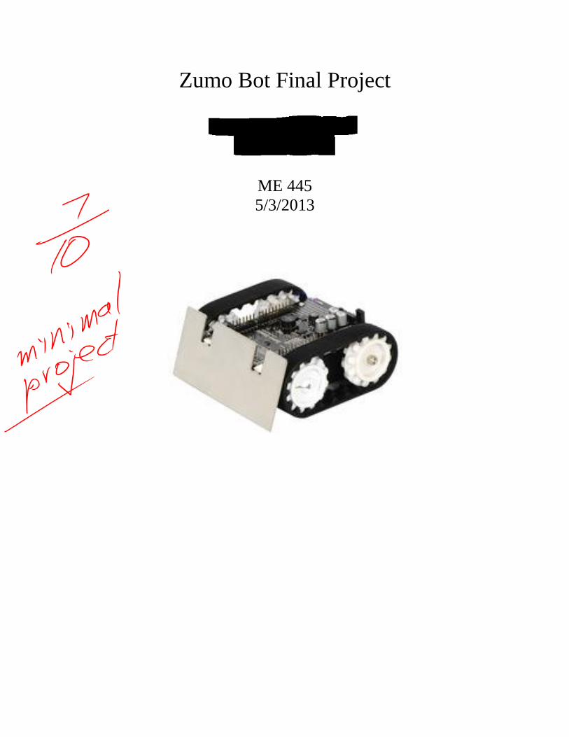
Zumo Bot Final Project
Dave Schmitthenner
Jim Sliwinski
ME 445
5/3/2013

1
Executive Summary The Pololu Zumo bot is small electronic robot platform that can be controlled through the use of
an Arduino Microcontroller Board. The Zumo bot contains two gear motors, two wheels
coupled on two pairs of silicone treads, and a stainless steel blade plow. All the necessary
infrared sensors, accelerometer, and magnetometer needed to function are incorporated into the
bot. However, headers can be soldered onto extra attachment points to incorporate other outside
sensors and devices to be used by the Zumo bot.
The team has constructed a battling robot that can compete against similar style robots. Two
other battling bots were created by other teams to contend for the class title of battle bot
champion during the finals week. The team’s robot included functions for detection of the other
battle bots through infrared sensors and a wedge mechanism intended to flip over the other bots.
A Pololu IR Beacon Transceiver was used by each of the teams to transmit and receive an
infrared signal to be used for the direction detection of the other robots. The incoming IR signal
of the other bots is processed by the Arduino code, determines whether the opponent is north,
east, south, or west of the team’s robot. Then a set of logic functions for each cardinal direction
tells the robot how to proceed. This sensor was to be mounted by all teams at a distance 4”
above the top of the Zumo bot with Arduino attached.
A Sharp GP2Y0A21 Distance Sensor and a Sharp GP2Y0D810Z0F Digital Distance Sensor
(10cm) were used to detect objects within a very close distance to the Zumo bot. The
GP2Y0A21 Sharp distance sensor, in conjunction with the Pololu IR Beacon Transceiver, was
used in the north, forward facing direction, to determine whether the robot was closing in on the
other robot, or potentially a wall while 3 Sharp GP2Y0D810Z0F Digital Distance Sensors
(10cm), in conjunction with the Pololu IR Beacon Transceiver, were used in the east, south, and
west facing sides to determine whether the opponent was attacking or the team’s robot was being
pushed too close to a wall.
An outer aluminum shell was created at the Learning Factory to protect the sensitive electrical
components of the sensors, the Arduino, and the Zumo, as well as providing a surface for the
sensors to be mounted onto.
Finally, the class competition was held on the second of May. A 4’x4’ arena was created for the
bots to battle. Each of the three team’s robots competed in a round robin style tournament with a
point system to determine which two teams would face off in the final match. 3 points were
awarded for flipping the opponent, 1 point was awarded for running the opponent into the wall,
and 1 point was taken away for running into the wall under the robot’s own control. The team’s
robot went 1-1 in the preliminary match but, after changes to code and design, was able to win
the final match.

2
Acknowledgements
The team would like to thank Dr. Sommer for providing the team with the necessary skills and
knowledge of electro-mechanical systems to make the completion of this project possible. The
team would also like to thank Mike Robinson for all his help throughout the course of the
semester with troubleshooting and helpful hints. Mike provided much valued assistance with the
final project by consulting with us about the progress of the project and, when needed, pointing
us in the right direction by explaining what we may be doing wrong. However, he only ever led
us on as much as we needed so that we could still solve the overall issues on our own and learn.
Also, thanks to Mike for providing the team with the Zumo bot and sensors, for building the
arena for the Zumo bots to battle, and for officiating the matches.

3
Table of Contents 1. Introduction ................................................................................................................................................ 5
1.1 Objectives ....................................................................................................................................... 5
1.2 Motivation ...................................................................................................................................... 6
2. Components ................................................................................................................................................ 6
2.1 Pololu IR Beacon Transceiver ........................................................................................................... 6
2.2 GP2Y0A21 Sharp Distance Sensor .................................................................................................... 6
2.3 Sharp GP2Y0D810Z0F Digital Distance Sensor 10cm ........................................................................ 7
2.4 Zumo Shield for Arduino.................................................................................................................. 7
3. Wiring and Programming .............................................................................................................................. 8
4. Mechanical Design .................................................................................................................................... 11
5. Conclusions and Recommendations ............................................................................................................ 12
6. APPENDICES .......................................................................................................................................... 14
APPENDIX A: HANDWRITTEN CODE .................................................................................................... 14
APPENDIX B: ARDUINO CODE .............................................................................................................. 15
APPENDIX C: DESIGN PROCESS ............................................................................................................ 19

4
......... 19

5
1. Introduction
1.1 Objectives
The team was to build a self-automated robot, using one of the given Zumo bots, to
compete against two other teams, building similar robots using the Zumo bots, at the end
of the semester. A Pololu IR Beacon Transceiver was required by each team to be
mounted 4” above the Zumo bot. This IR beacon was to be used to determine the
direction in which the opposing robot was in relation to team’s robot. The robot was also
to utilize other sensors, servos, etc. to improve its battling capabilities. IR sensors were
to detect the walls of the arena and a weapon, or some other device, was to flip and/or
plow the opposing robot.

6
1.2 Motivation
The motivation for this project came from the old competition that used to be on
television, called BattleBots. Creating a self-automated robot that detects and seeks out
another robot while attempting to dismantle the other bot using moving parts seemed like
a perfect fit for the wide range scope of the final project.
2. Components
2.1 Pololu IR Beacon Transceiver
The IR Beacon Transceiver can be seen below in Figure 1. It works via infrared
emitters on its top face that another beacon could read, and sensors, seen in black, that
sense another beacon’s signal. Whichever sensor reads the IR signal, it’s corresponding
pin outputs a low signal, and an LED on the top face lights up. This sensor works quite
well at long range, but too close to another one and the sensors pick up false signals. For
this reason, shorter range methods had to be implemented.
Figure 1 - IR Beacon
2.2 GP2Y0A21 Sharp Distance Sensor
The distance sensor is in Figure 2. It senses anything in front of it up to about 32
in. and outputs a voltage according to the graph in figure 2.

7
Figure 2 - Distance Sensor and Graph
2.3 Sharp GP2Y0D810Z0F Digital Distance Sensor 10cm
This digital distance sensor is in Figure 3. It senses anything in front of it within
10 cm and outputs a low if any object is within 10 cm of the sensor.
Figure 3 - Digital distance sensor
2.4 Zumo Shield for Arduino
The critical component was the Zumo Shield. Pololu has a library that allows for
easy control of the sumo bot. Using simple commands, the arduino can output a signal

8
that tells each motor a value from -400 to 400. Negative numbers represent reverse, and
the magnitude is the speed, 400 being 100%. The Zumo bot is in Figure 4.
Figure 4 - Zumo Bot
3. Wiring and Programming
The wiring for this project was quite simple. All the components mentioned above required
5V and ground, fortunately the Zumo shield had pre-connected headers that connected to the
Arduino 5V and ground, which was helpful in keeping everything at the same ground. The
analog distance sensor was connected to the A0 pin, and the rest of the sensing components
connected to digital pins. Care was taken to avoid pins 1 and 0 because the Arduino uses these
for serial communication. Also, the Zumo shield uses pins 7-10 for its motors, so use of those
pins were avoided as well.
A flowchart for the programming can be seen in Figure 5. The code was split into long range
and short range. If none of the short range sensors were low, then the opponent was over 10cm
away and the longrange() function was used. If any of the sensors were tripped, the closerange()
function went into effect.
The long range function worked by reading which direction the IR beacon was reading, point
the bot toward it, and then move toward it.
The short range function worked based on what sensors were blocked. If the front was the
only one blocked, it was assumed that this was the opponent, and the robot moved forward. If the
robot was blocked on more than one side, one of these must be a wall, and to avoid running into
it the robot moved away from the blocked side, and moved forward until one of the blocks
disappeared. If it was only blocked on one side other than north, it would move away from the
block and move forward. Eventually, this would either result in ramming the opponent into a
wall, or moving away from any blocks until none were detected, and the long range function
would go back into effect.
The movement functions were created to make it easier to tell the robot how to move. For
example, a spinLeft() function would spin the right motor forward and the left backward. The
full code can be seen in the Appendix.

9
Figure 5 - Overall Function

10
Figure 6 - Long Range Function
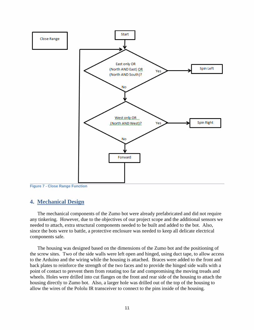
11
Figure 7 - Close Range Function
4. Mechanical Design
The mechanical components of the Zumo bot were already prefabricated and did not require
any tinkering. However, due to the objectives of our project scope and the additional sensors we
needed to attach, extra structural components needed to be built and added to the bot. Also,
since the bots were to battle, a protective enclosure was needed to keep all delicate electrical
components safe.
The housing was designed based on the dimensions of the Zumo bot and the positioning of
the screw sites. Two of the side walls were left open and hinged, using duct tape, to allow access
to the Arduino and the wiring while the housing is attached. Braces were added to the front and
back plates to reinforce the strength of the two faces and to provide the hinged side walls with a
point of contact to prevent them from rotating too far and compromising the moving treads and
wheels. Holes were drilled into cut flanges on the front and rear side of the housing to attach the
housing directly to Zumo bot. Also, a larger hole was drilled out of the top of the housing to
allow the wires of the Pololu IR transceiver to connect to the pins inside of the housing.

12
Figure 8 - Aluminum Housing
Additionally, the offensive component was also made from thin aluminum sheet metal. It
was formed into the shape of a V-Wedge and connected to the housing at the base of the front,
north facing side, of the Zumo bot using duct tape and superglue. This wedge was to act as the
means of flipping and/or plowing the other robots.
Finally, the electrical components and sensors were attached to the housing. The 3 Sharp
GP2Y0D810Z0F Digital Distance Sensors (10cm) were attached to the housing via duct tape.
Two small holes were drilled into the front face to attach the Sharp GP2Y0A21 Distance Sensor
with screws. The Pololu IR beacon transceiver was also attached to the top of the housing via
duct tape.
5. Conclusions and Recommendations
We learned quite a lot about the challenges involved in making an autonomous robot.
Powering everything proved a challenge, and pulling around as much weight as we did seemed
to drain the battery. We learned the most about logic in general. Figuring out what to do in
certain situations so that it would put itself in a planned position was a challenge. For example, if
the robot was blocked on the north and south, in order to avoid hitting a wall it should turn left.
Now it is blocked on the east and west, so it should move forward until one of the blocks
disappears. Assuming the opponent was to the east, that block would disappear, now the robot
needs to turn right, so the wall is to the south, then move forward. This analysis needed to be
done for every possible combination. This can be seen in the appendix.
The biggest challenge was dealing with blind spots. At times, the other robot was in between
the sensing areas of the close range directional sensors, and because of the proximity, the IR
beacon was of no use. In addition, the programming assumed only 4 possible directions, north
south east and west. In reality, the robot has 360 degrees of rotation. This led to the robot not

13
approaching its opponent head on, but at an askew angle. This could potentially be fixed with
either overcompensating in the code, or by using better sensing methods.
Some improvements that could have been implemented with more time are to use the motor’s
variable speeds. For example going slowly when far away from an opponent, and ramping up
speed as the opponent gets closer. The robot also has the ability to either spin on its own axis, or
rotate in a larger circle, we did not take advantage of this, but it could be implemented. Lastly,
the use of other servomotors could be implemented in the forms of flippers, pushers, re-
uprighters, etc.

14
6. APPENDICES
APPENDIX A: HANDWRITTEN CODE

15
APPENDIX B: ARDUINO CODE
#include <ZumoMotors.h>
ZumoMotors motors;
int N; //long range variables
int E;
int S;
int W;
int n=5; //long range pins
int e=4;
int s=3;
int w=2;
int closeE; //short range variables
int closeS;
int closeW;
int closee=6; //short range pins
int closes=11;
int closew=12;
int enable=13; //beacon enable pin
int range; //range variable
void setup()
//set pin modes
pinMode(enable,OUTPUT);
pinMode(A0,INPUT);
pinMode(n,INPUT);
pinMode(e,INPUT);
pinMode(s,INPUT);
pinMode(w,INPUT);
pinMode(closee,INPUT);
pinMode(closes,INPUT);
pinMode(closew,INPUT);
Serial.begin(9600);
// uncomment one or both of the following lines if your motors' directions need to be flipped
motors.flipLeftMotor(true);
//motors.flipRightMotor(true);
void loop()
// read everything
digitalWrite(enable,HIGH);
N=digitalRead(n);
E=digitalRead(e);
S=digitalRead(s);
W=digitalRead(w);
range=analogRead(A0);
closeE=digitalRead(closee);
closeS=digitalRead(closes);

16
closeW=digitalRead(closew);
if ((range>250)||(closeE==0)||(closeW==0)||(closeS==0))
//if any close range sensor goes off, go to close range
closeRange();
Serial.print("close ");
Serial.print(range);
Serial.print(" ");
Serial.print(closeE);
Serial.print(" ");
Serial.print(closeS);
Serial.print(" ");
Serial.println(closeW);
else
//otherwise go to long range
longRange();
Serial.print("long ");
Serial.print(range);
Serial.print(" ");
Serial.print(N);
Serial.print(" ");
Serial.print(E);
Serial.print(" ");
Serial.print(S);
Serial.print(" ");
Serial.println(W);
//long and short range functions
void longRange()
// call functions to turn towards beacon
if (N==0)
north();
else if (E==0)
east();
else if (S==0)
south();
else if (W==0)
west();

17
void closeRange()
// short range operations
if ( ((closeE==0)&&(((range>250)||(closeW==0)||(closeS==0))==0)) || ((range>250)&&(closeE==0)) ||
((range>250)&&(closeS==0)))
//if only east, northeast, or north/south are blocked, turn left
Serial.print(" spinleft ");
else if ( ((closeW==0)&&(((range>250)||(closeE==0)||(closeS==0))==0)) || ((range>250)&&(closeW==0)))
//if only west, or northwest are blocked, turn right
Serial.print(" spinRight ");
else // otherwise go forward
Serial.print(" ramrod ");
// directional functions
void north()
// attacks
Serial.print(" ramrod ");
void east()
// turns right until the beacon is not east
Serial.print(" spinRight ");
void west()
// turns left until the beacon is not west
Serial.print(" spinleft ");
void south()
//turns left until beacon is not south
Serial.print(" spinleft ");
// sumo bot functions
void spinLeft()
//spins left
motors.setLeftSpeed(-400);
motors.setRightSpeed(400);

18
void spinRight()
//spins right
motors.setLeftSpeed(400);
motors.setRightSpeed(-400);
void halt(int t)
//full stop for t time
motors.setRightSpeed(0);
motors.setLeftSpeed(0);
delay(t);
void ramrod()
// runs forward at full speed
motors.setRightSpeed(400);
motors.setLeftSpeed(400);
void backup()
//backward at full speed
motors.setRightSpeed(-400);
motors.setLeftSpeed(-400);

19
APPENDIX C: DESIGN PROCESS

20

21

22

23
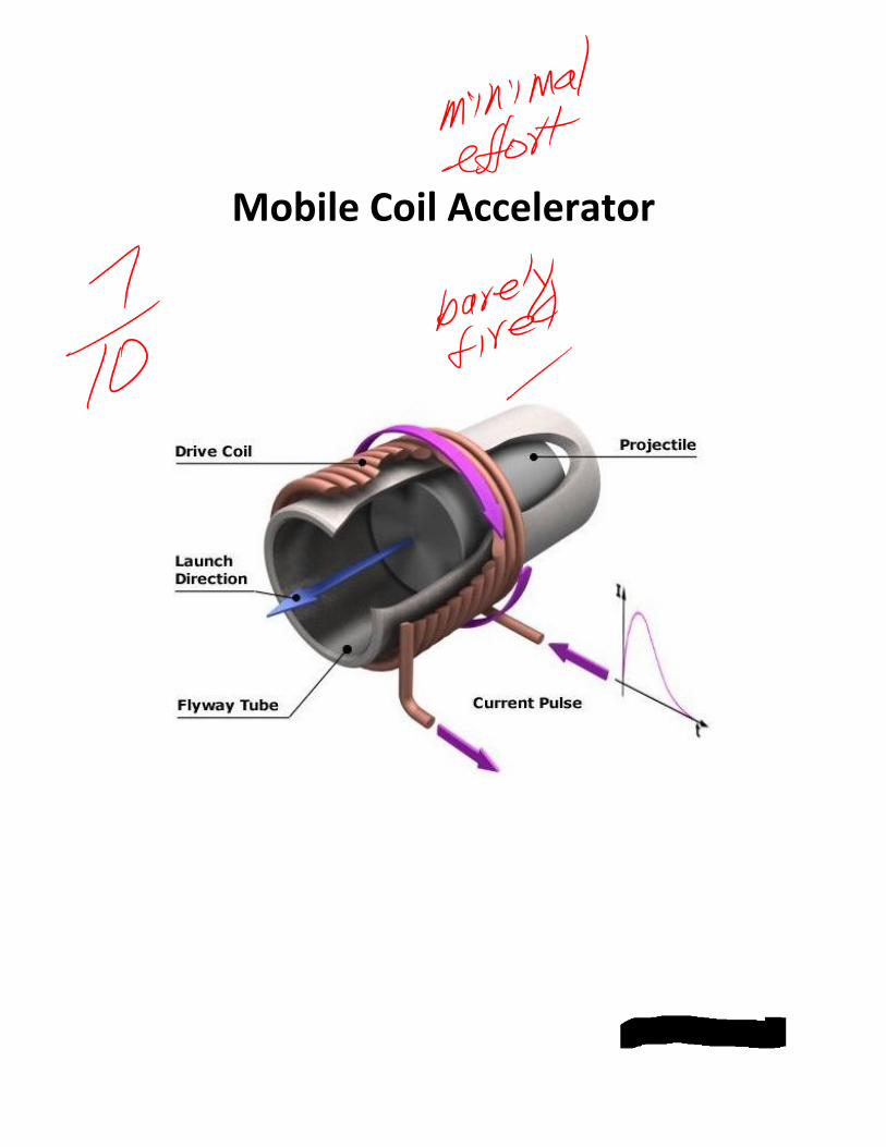
Nazareno | Shemro 0
Mobile Coil Accelerator

Nazareno | Shemro 1
Group Number 6
Nathaniel Nazareno
Owen Shemro
ME445: Microcomputer Interfacing
May 3, 2013

Nazareno | Shemro 2
Executive Summary
The Mobile Coil Accelerator has been completed to a minimally functional level. Basic firing of the accelerator, basic movements and automation of the motorized vehicle, and component integration has been achieved. The accelerator is not yet optimized and still needs an automatic charging system. The vehicle control needs to be reworked as it is not capable of operating in reverse.
Acknowledgement
We would like to thank mike for providing the parts needed for the project and for his invaluable advice and ability to show us all the things we did terribly wrong. Our project would never have functioned without his guidance.

Nazareno | Shemro 3
Table of Contents Introduction ..................................................................................................................................................4
Problem Statement...................................................................................................................................4
Motivation.................................................................................................................................................4
Background Information ...............................................................................................................................4
Project Planning ........................................................................................................................................4
Initial Design Concept ...............................................................................................................................5
Concept Development ..............................................................................................................................5
Bill Of Materials.........................................................................................................................................5
Detailed Design .............................................................................................................................................6
Circuit Diagram .........................................................................................................................................6
Mechanical Design ....................................................................................................................................8
Hardware ....................................................................................................................................................10
Lego DC Motor ........................................................................................................................................10
Dual Motor Driver ...................................................................................................................................11
Servo and Sensor ....................................................................................................................................11
Coil Accelerator.......................................................................................................................................13
Conclusion...................................................................................................................................................13
What we learned.....................................................................................................................................13
What could be improved ........................................................................................................................13
Appendix .....................................................................................................................................................15

Nazareno | Shemro 4
Introduction
Problem Statement Since the dawn of man, humans have loved to run around and throw stuff at other stuff. We started throwing rocks and spears, but in this modern age, we get machines to do it for us. To create a machine that can move around and shoot at stuff, we must create a system to control a series of motors and servos, as well as charging and firing a coil accelerator system. To do this, we will create a circuit to control the coil accelerator and a motorized vehicle through an arduino.
Motivation Our instructor, Professor Sommers has always talked about how he has created these special robots made to transport items through rough terrain. He has also made robots that were capable of shooting paintball accelerators. Through the ideas given to us by our instructor, we have decided to create our own version of what he has done. It will be a small scale version of what he has done but will use a coil accelerator rather than a paintball accelerator.
There was also a video we found online dealing with coil accelerator. It was very entertaining to watch the person create his own accelerator as well as watching the speed at which the projectile released. This accelerator was very simple to create and wanted to make our own version.
Background Information
Project Planning The plan for the project was to individual creates each section. The 2 sections for the project would be the coil accelerator and the vehicle. We would need a coil accelerator that will be powered through capacitors that will be able to hold about 50Vs through 9V batteries and a vehicle that will be remote controlled using a dual motor driver.

Nazareno | Shemro 5
These two sections are somewhat divided between each group member. But while each member had their own section, the work had to be done together to give input and ideas to improve the end goal. This was decided because it would get more work done in less time since we could simply hook the arduino up to both components and run a program using 1 arduino.
This may see to split the knowledge that could be obtained from division of labor, we saw to it that each member understand each part of all the respective sections. The main factor we wanted out of this project is to understand coil accelerators and remote or autonomous robotic vehicles.
Initial Design Concept The initial design of the product only dealt with the coil accelerator. We wanted an accelerator that would be powerful enough to piece cardboard. The problem with this was that we did not think it was challenging enough. We could easily wire together the parts to make a strong coil accelerator but to step up the project we decided to add the vehicle component. At first we did not decide on a vehicle only because of the possible problems we would face. These problems would deal the ability of the accelerator to charge the capacitors on its own, remote controlling the vehicle, or even coding it. We decided on the vehicle because of the challenge that it would give us as well as the concepts we could possibly learn from these extra section of the project.
Concept Development The concept was first acknowledged through a view we found online. There was a video that caught our attention through the methods of a coil accelerator and gave us the inspiration to design our own product with a vehicle design to give it a larger scale. While his idea own showed the coil accelerator, we decided to expand upon the idea to give us a defense system that would be able to shoot projectiles through a remote controlled vehicle.
Bill Of Materials
Parts Quantity Vendor Price (each)
Arduino Uno 1 Jameco $29.99
Lego Motors 2 Lego $19.99

Nazareno | Shemro 6
Sharp Distance Sensor 2Y0A02
1 DHGate $11.97
GWS S03N Standard Servo
1 RobotShop $10.00
50V 3300 uF Caps 4 ElectronicSurplus $3.00
L293DNE 1 Digikey $3.50
SN74LS04N 1 Mouser $0.46
1N5408 Diode 1 Mouser $0.25
9V Batteries 5 MedicBatteries $1.30
FQP30N06L MOSFET 1 Mouser $0.47
Table 1: Bill of Materials
Detailed Design
Circuit Diagram
The entire project was able to use only 1 arduino to control all the parts of the vehicle as well as the coil accelerator. This was through the use of two different power supplies, one for the vehicle and another to charge the capacitors.

Nazareno | Shemro 7
Figure 1: Circuit Diagram
The simple vehicle circuit can be seen in Figure 1. It shows the use of the arduino connected different components. The distance sensor is connected to the analog input while the servo and dual motor driver, which is connected to the 2 motors, is connected to the digital pins.

Nazareno | Shemro 8
Figure 2: Vehicle Component Diagram
Figure 2 gives you a view that allows you to see each component and how they are connected to each other on the breadboard and arduino. In this circuit you can see that we are missing the dual motor driver. This was created using the program Fritzing. It has limited parts but gives you a better visualization of the real circuit. Because of this, we had to make do with the parts given. You can see that this circuit contains all parts that help the vehicle run. For the motors, the black and white wires represent the power wires used to control the motors direction and speed. The yellow wires represent the digital or analog inputs which are connected to the arduino. The red and black wires show the power and ground. We have also implemented a switch to assist with its autonomous mode.
Mechanical Design

Nazareno | Shemro 9
Figure 3: Vehicle Prototype
Figure 4: Coil Accelerator Prototype
The main component of our design will use Lego pieces. We decided on this because of how we are easily able to structure the Lego pieces to our design. The pieces will be used to create two levels to hold all the hardware of the coil accelerators well as the hardware of the vehicle itself.
The vehicle design will contain 2 wheels which are each powered by its own motor. The wheels will be located in near the middle of the vehicle so that it has more maneuverability by allowing it to rotate on its own axis. To keep balance, we simply placed pieces in the front and back of the vehicle to level it.

Nazareno | Shemro 10
Hardware
Figure 5: Lego Motor
Lego DC Motor Previously in this class we learned about how to control a Lego motor with its encoder. A Lego motor is basically a DC motor. This gave us the ability to control the angle the motor would move as well as the speed in which the motor will move. We did not use the encoders but rather the power pins to only control the direction the motor will move but having these motors gave us that option. This is why he decided to use Lego motors. Having the background knowledge we could have implemented the encoder to have better control of what the vehicle does.
Figure 6: Dual Motor Driver

Nazareno | Shemro 11
Dual Motor Driver Another part we have used in lab would be the Dual Motor Driver which can be used to control the speed and direction of two motors. It uses a L293DNE and SN74LS04N chips. The L293DNE chip contains 4 half H drivers which are used to control the direction of the output current. It using 1 half H driver provides a unidirectional flow while using 2 using allows for a bidirectional flow. The SN74LS04N chip contains hex inverters which are basically used to assist the operation of the entire product.
Figure 7: Accelerator Servo & Distance Sensor
Servo and Sensor The distance sensor we used is a Sharp Distance Sensor 2Y0A02. It is a long range sensor that would be used to either maneuver through obstacles or find targets. Below is that formula for the serial output of the sensor.
Distance (cm) = 9462 / (SensorValue ‐ 16.92)
This formula is only good for a sensor value between 80 and 490. With this distance sensor, the closer an object is to it, the higher the serial output. The problem with this sensor is that when it senses objects that are too close, the value that it outputs decreases. It has a peak were after a certain distance, the sensor value would decrease instead of increase while sensing an object getting closer. This sensor would have been mounted on the servo we used to give us a field of vision.

Nazareno | Shemro 12
The servo we used was a GWS S03N Standard Servo has a high torque compared to other similar servos. It outputs about 56 oz.‐in at a speed of 0.18 seconds per 60 degrees of motion at 6 V. The coil accelerator was mounted on the servo to give a better range of attack. The servo was placed near the front of the vehicle for a rotating distance sensor and coil accelerator.
Figure 8: Battery Bank
Figure 9: Capacitor Bank
Figure 10: Accelerator Coil

Nazareno | Shemro 13
Coil Accelerator The coil accelerator itself is a hand wound solenoid consisting of thin magnet wire wound around a metal sheet and a plastic straw. Another metal sheet was wrapped around the outside of the coil and taped together with duct tape. Using the metal sheet helped to focus the magnetic field into the center of the solenoid to increase the power output. Also, using very thin magnet wire allowed us to keep the coils closer to the center of the solenoid, which strengthened the magnetic field created by the coil.
Conclusion
What we learned For the vehicle section we learned that it would have been better to complete the circuit before deciding on the design of the vehicle. We prebuilt the vehicle before most of the wiring was done so we were not sure how much space would be needed to fit all the components. I gave it 2 levels thinking that would be enough to hold all the parts while long wires could be held by the holes of the Lego pieces. The Lego vehicle we created did not have enough space to compensate for the wires as well as large parts such as the capacitors. For future designs, we have learned to design the vehicle around the main circuit diagram to consider all the options and give enough space for all the parts and wires.
For the coil accelerator, we learned that using a metal shield around the coil helped to increase the power output. We also learned that timing the length of the pulse sent to the coil is very important and varies based on several variables including the mass of the projectile, the starting voltage of the capacitors, and other factors in the circuitry. Ideally we would have liked to have optimized the pulse timing once the circuit was complete and we were using a single projectile consistently.
What could be improved There are many ways in which we can improve this vehicle to give it its most optimal settings. Our current design does not incorporate the servo and the distance sensor since we use switches to move the individual motors. To improve this we could either create a remote controlled robot or one that can move autonomously. For the remote controlled robot, we could simply incorporate a controlled into our arduino like we do with our switches but in a wireless manner. For the autonomous robot, it would have to incorporate more code. We would have mounted both the coil accelerator as well as the distance sensor so that we can have the distance sensor have a field of vision. We would have liked to code the vehicle so it does a 180 degree scan of an area trying to find any objects that are too close to it. If it does

Nazareno | Shemro 14
find an object, the servo would turn towards that object to get ready to fire. The arduino would then power a transistor to charge the capacitors up to at least 30 volts, and then have another transistor that would be used to release it which would fire the coil accelerator.
For the coil accelerator, we were unable to create a charging circuit that could be operated by the arduino. Ideally the charging circuit would include a voltage divider where the arduino could read the state of charge and charge the capacitors automatically.
The coil accelerator also could be improved by using an infrared sensor and emitter to detect when the projectile has passed through the coil so that the pulse timing would not have to be optimized for each situation and would instead react immediately. Ultimately, we would like to have added additional coils to get the projectile going even faster.

Nazareno | Shemro 15
Appendix 1N5408 Diode
http://www.fairchildsemi.com/ds/1N/1N5408.pdf

Nazareno | Shemro 16
Hex Inverter SN74LS04N

Nazareno | Shemro 17
http://www.datasheetcatalog.org/datasheets/90/487903_DS.pdf
Motor Driver L293DNE

Nazareno | Shemro 18
http://www.datasheetcatalog.org/datasheet2/f/0xt5w1akzx8dd88ewqdxi35wa9py.pdf
FQP30N06L MOSFET
http://www.fairchildsemi.com/ds/FQ/FQP30N06L.pdf

Nazareno | Shemro 19
Arduino Code:
int pwmMotor1 = 3;
int pwmMotor2 = 5;
int driveMotor1 = 2;
int driveMotor2 = 4;
int chargeSwitch = 10;
int fireSwitch = 13;
int trigger = 6;
int charger = 7;
#include <Servo.h>
Servo myservo; // create servo object to control a servo
// a maximum of eight servo objects can be created
int pos = 0; // variable to store the servo position
int distancePin = A0;
void setup()
// put your setup code here, to run once:
Serial.begin (9600);
pinMode(driveMotor1,OUTPUT);
pinMode(driveMotor2, OUTPUT);
pinMode(chargeSwitch,OUTPUT);
pinMode(fireSwitch,OUTPUT);

Nazareno | Shemro 20
pinMode(trigger,INPUT_PULLUP);
pinMode(charger,INPUT_PULLUP);
myservo.attach(12); // attaches the servo on pin 9 to the servo object
void loop()
// put your main code here, to run repeatedly:
int distance = analogRead(distancePin);
Serial.println(distance);
if (digitalRead(trigger) == LOW)
digitalWrite (fireSwitch,HIGH);
delay (50);
digitalWrite (fireSwitch,LOW);
delay(1000000);
if (distance < 500 && distance > 200)
motor(0,1,0,0);
delay(500);
else

Nazareno | Shemro 21
motor(0,1,0,1);
// for(pos = 0; pos < 180; pos += 1) // goes from 0 degrees to 180 degrees
// // in steps of 1 degree
// myservo.write(pos); // tell servo to go to position in variable 'pos'
// delay(15); // waits 15ms for the servo to reach the position
//
// for(pos = 180; pos>=1; pos‐=1) // goes from 180 degrees to 0 degrees
//
// myservo.write(pos); // tell servo to go to position in variable 'pos'
// delay(15); // waits 15ms for the servo to reach the position
//
void motor(float motorSpeed1, float motorDir1, float motorSpeed2, float motorDir2)
motorSpeed1 = 255‐motorSpeed1;
analogWrite(pwmMotor1,motorSpeed1);
if (motorDir1 > 0)
digitalWrite(driveMotor1,LOW);
Nazareno | Shemro 22
else
digitalWrite(driveMotor1,HIGH);
motorSpeed2 = 255‐motorSpeed2;
analogWrite(pwmMotor2,motorSpeed2);
if (motorDir2 > 0)
digitalWrite(driveMotor2,LOW);
else
digitalWrite(driveMotor2,HIGH);


