18
ME598 Introduction to Robots Lab 2 Report Group E Group Members: Renjie Xie David Harman Hao Wu Jiachuan Peng Submission Date: 3/28
| Date post: | 15-Apr-2017 |
| Category: |
Documents |
| Upload: | renjie-xie |
| View: | 86 times |
| Download: | 0 times |
ME598 Introduction to Robots
Lab 2 Report
Group E
Group Members:
Renjie Xie
David Harman
Hao Wu
Jiachuan Peng
Submission Date: 3/28
Part 0: Configure and Test RAIS System with Manipulator
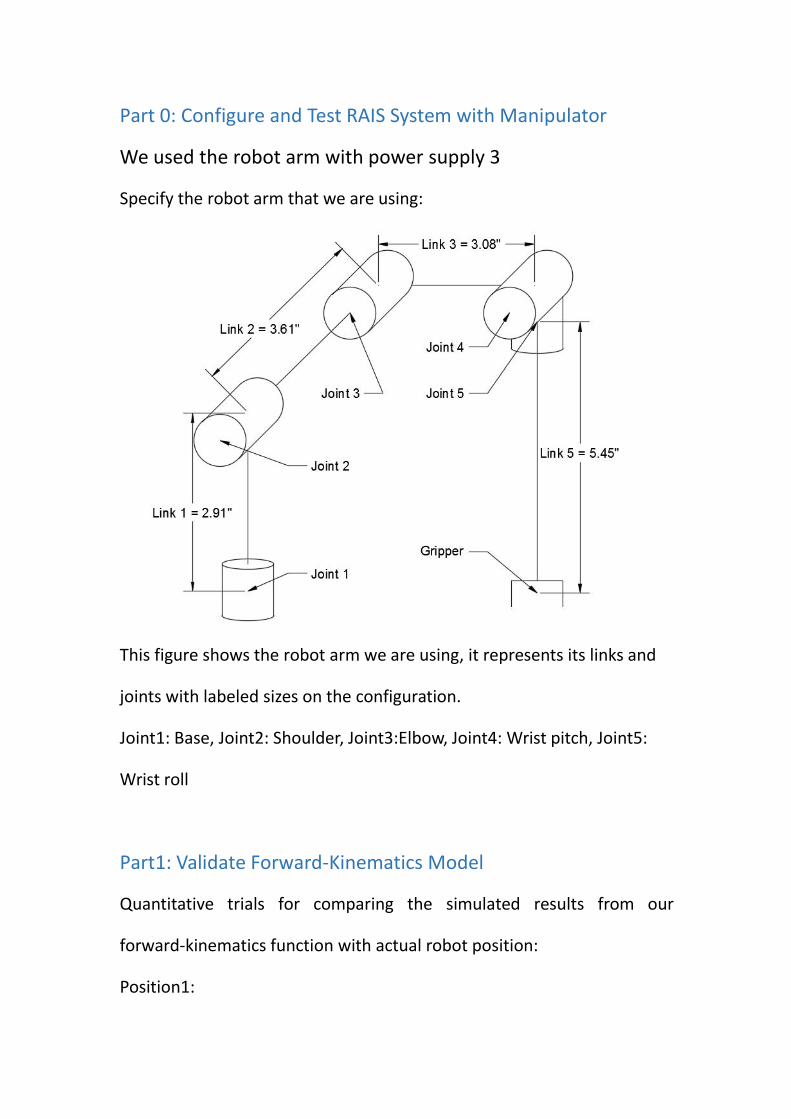
We used the robot arm with power supply 3
Specify the robot arm that we are using:
This figure shows the robot arm we are using, it represents its links and
joints with labeled sizes on the configuration.
Joint1: Base, Joint2: Shoulder, Joint3:Elbow, Joint4: Wrist pitch, Joint5:
Wrist roll
Part1: Validate Forward-Kinematics Model
Quantitative trials for comparing the simulated results from our
forward-kinematics function with actual robot position:
Position1:
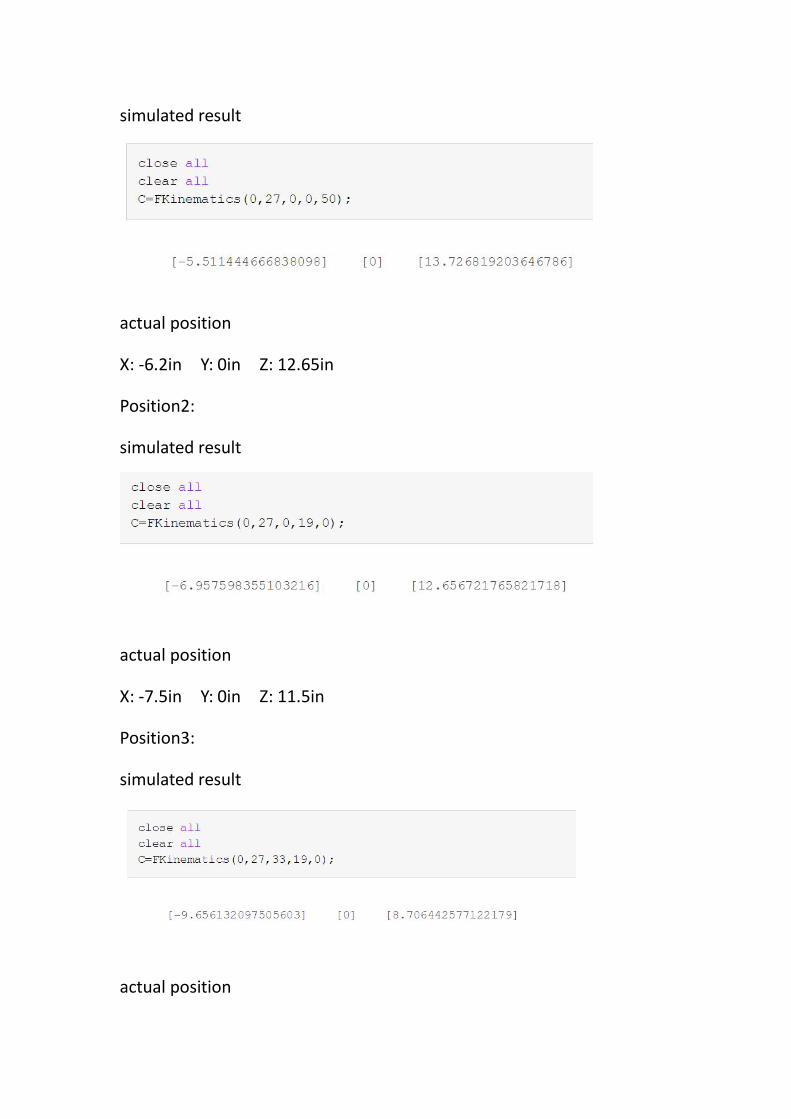
simulated result
actual position
X: -6.2in Y: 0in Z: 12.65in
Position2:
simulated result
actual position
X: -7.5in Y: 0in Z: 11.5in
Position3:
simulated result
actual position

X: -10.1in Y: 0in Z: 7in
Position4:
simulated result
actual position
X: -10in Y: 0in Z: 6.75in
Position5:
simulated result
actual position
X: -10.2in Y: -1.6in Z: 7.2in
Position6:
simulated result
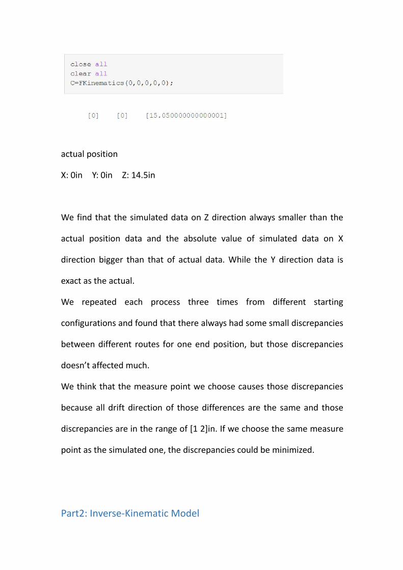
actual position
X: 0in Y: 0in Z: 14.5in
We find that the simulated data on Z direction always smaller than the
actual position data and the absolute value of simulated data on X
direction bigger than that of actual data. While the Y direction data is
exact as the actual.
We repeated each process three times from different starting
configurations and found that there always had some small discrepancies
between different routes for one end position, but those discrepancies
doesn’t affected much.
We think that the measure point we choose causes those discrepancies
because all drift direction of those differences are the same and those
discrepancies are in the range of [1 2]in. If we choose the same measure
point as the simulated one, the discrepancies could be minimized.
Part2: Inverse-Kinematic Model
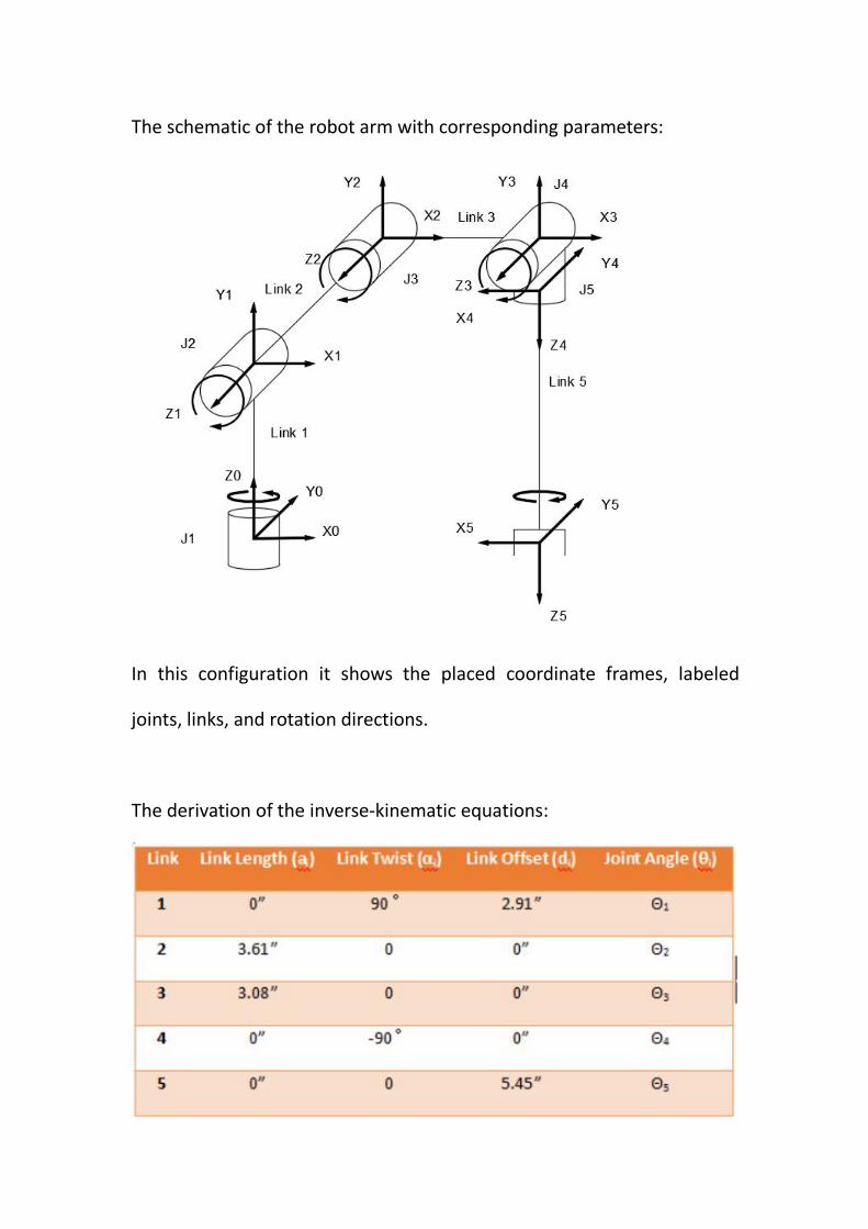
The schematic of the robot arm with corresponding parameters:
In this configuration it shows the placed coordinate frames, labeled
joints, links, and rotation directions.
The derivation of the inverse-kinematic equations:

DH Parameters
The final transforming matrix is:
5*4*3*2*1 AAAAAT
Thus

Since the griper could be assumed to be pointing downward all the time,
the transforming matrix from frame 0 to frame 5 shall fulfill the following
form:
T'=
1000z100y0cossinx0sincos-
g
g
g
(In which θ equals θ1-θ5)
Thus the inverse kinematic equations are (5 variables requires 5
equations at least):
-cosθ=c1c234c5+s1s5; sinθ=-c1c234s5+s1c5;
-c1s234=0; -s1s234=0; -c234=-1; -s234c50; s234s5=0;
-d5c1s234+a3c1c23+a2c2c1=xg;
-d5s1s234+a3c1c23+a2c2s1=yg;
-d5c234-a3s23+d1-a2s2=zg;
Examples to check the output joints value:
1.

2
3.
The MATLAB code in the appendix.

Part3: Basic Path Planning
1. From the position (0, 4) to (-4, 0)
The path from the text file
90 0 90 78 0 50
90 0 90 78 0 0
7 0 90 15 0 0
7 0 90 78 0 0
7 0 90 78 0 50
0 0 0 0 0 50
The robot arm end-effector arrives at the position (0, 4) by inputting
each joint value (90 0 90 78 0), then closes the gripper and
moves to position (-4, 0) by inputting joint value (7 0 90 15 0)and
(7 0 90 78 0 0). Open the gripper to put the bolt and return to
home position (joint value: (0 0 0 0 0)).
2. From the position (-4, 0) to (0, -4)
The path from the text file
5 0 90 78 0 50
5 0 90 78 0 0
-90 0 90 15 0 0
-85 0 90 78 0 0
-85 0 90 78 0 50

0 0 0 0 0 50
The robot arm end-effector arrives at the position (-4, 0) by inputting
joint value (5 0 90 78 0 )(because the robot arm is not absolute
vertical, thus the first joint value is 5 instead of 0 for compensating the
tilt), then closes the gripper and moves to position (0, -4) by inputting
joint value (-90 0 90 15 0) and (-85 0 90 78 0 0). Open
the gripper to put the bolt and return to home position (joint value: (0
0 0 0 0)).
3. From the position (0, 4) to (-4, 0) and continue from the position (-4, 0)
to (0, -4)
The path on the text file
90 0 90 78 0 50
90 0 90 78 0 0
7 0 90 15 0 0
7 0 90 78 0 0
7 0 90 78 0 50
7 0 90 78 0 0
-90 0 90 15 0 0
-85 0 90 78 0 0
-85 0 90 78 0 50
0 0 0 0 0 50

The robot arm reaches the position (0, 4) first and closes the gripper to
catch the bolt and moves to the position (-4, 0), open the gripper to
release the bolt. Then, closes the gripper and sends the bolt to the
position (0, -4). Return to home position at the end.
We have tested each path three times and found that we could catch the
bolt and move to the destination almost accurately every time.
The path is inferred by combining the two paths mentioned above since
the intermediate configuration connecting the end position of first path
with the start position of second path, the robot arm could also move
continuously. Thus the path could the gathered to create a compound
path.
The video address
https://youtu.be/uMU8d3zsCS0
Part 4: multiple object path planning
Specify the obstacle starting positions
1. (3, 4.5) 2. (5, 3) 3.(2, 6)
The bin position
(4, 9)
The path on the text file

59 10 80 67 0 50
59 10 80 67 0 0
59 10 51 67 0 0
-66 31 21 45 2 0
-66 31 21 45 2 50
-34 31 21 45 2 50
-29 23 58 80 2 50
-29 23 58 80 2 0
-34 31 21 45 2 0
-66 31 21 45 2 0
-66 31 21 45 2 50
-86 31 21 45 2 50
-86 28 35 89 2 50
-70 28 35 89 2 50
-70 35 39 89 2 50
-70 35 39 89 2 0
-81 15 39 89 2 0
-86 21 40 37 2 0
-67 22 23 62 2 0
-67 22 23 62 2 50
0 0 0 0 0 50
First move the robot arm end-effector to the position 1 (3, 4.5) by
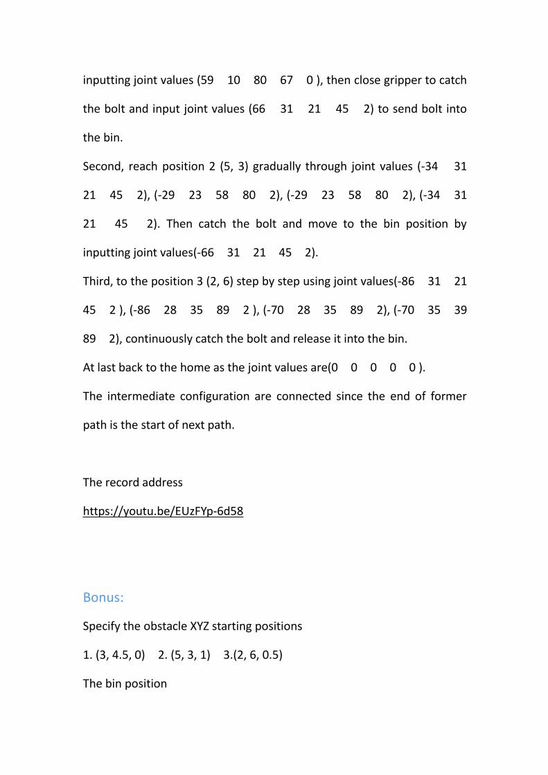
inputting joint values (59 10 80 67 0 ), then close gripper to catch
the bolt and input joint values (66 31 21 45 2) to send bolt into
the bin.
Second, reach position 2 (5, 3) gradually through joint values (-34 31
21 45 2), (-29 23 58 80 2), (-29 23 58 80 2), (-34 31
21 45 2). Then catch the bolt and move to the bin position by
inputting joint values(-66 31 21 45 2).
Third, to the position 3 (2, 6) step by step using joint values(-86 31 21
45 2 ), (-86 28 35 89 2 ), (-70 28 35 89 2), (-70 35 39
89 2), continuously catch the bolt and release it into the bin.
At last back to the home as the joint values are(0 0 0 0 0 ).
The intermediate configuration are connected since the end of former
path is the start of next path.
The record address
https://youtu.be/EUzFYp-6d58
Bonus:
Specify the obstacle XYZ starting positions
1. (3, 4.5, 0) 2. (5, 3, 1) 3.(2, 6, 0.5)
The bin position

(4, 9)
The path on the text file
59 10 80 67 0 50
59 10 80 67 0 0
59 10 51 67 0 0
-66 31 21 45 2 0
-66 31 21 45 2 50
-29 21 38 34 2 50
-29 21 38 98 2 50
-29 21 38 98 2 0
-29 12 31 48 2 0
-64 18 40 39 2 0
-64 18 40 39 2 50
-89 18 40 39 2 50
-89 7 62 70 2 50
-70 7 62 70 2 50
-70 14 68 66 2 50
-70 14 68 66 2 0
-85 14 59 66 2 0
-85 2 40 66 2 0
-65 20 30 38 2 0
-65 20 30 38 2 50
0 0 0 0 0 50
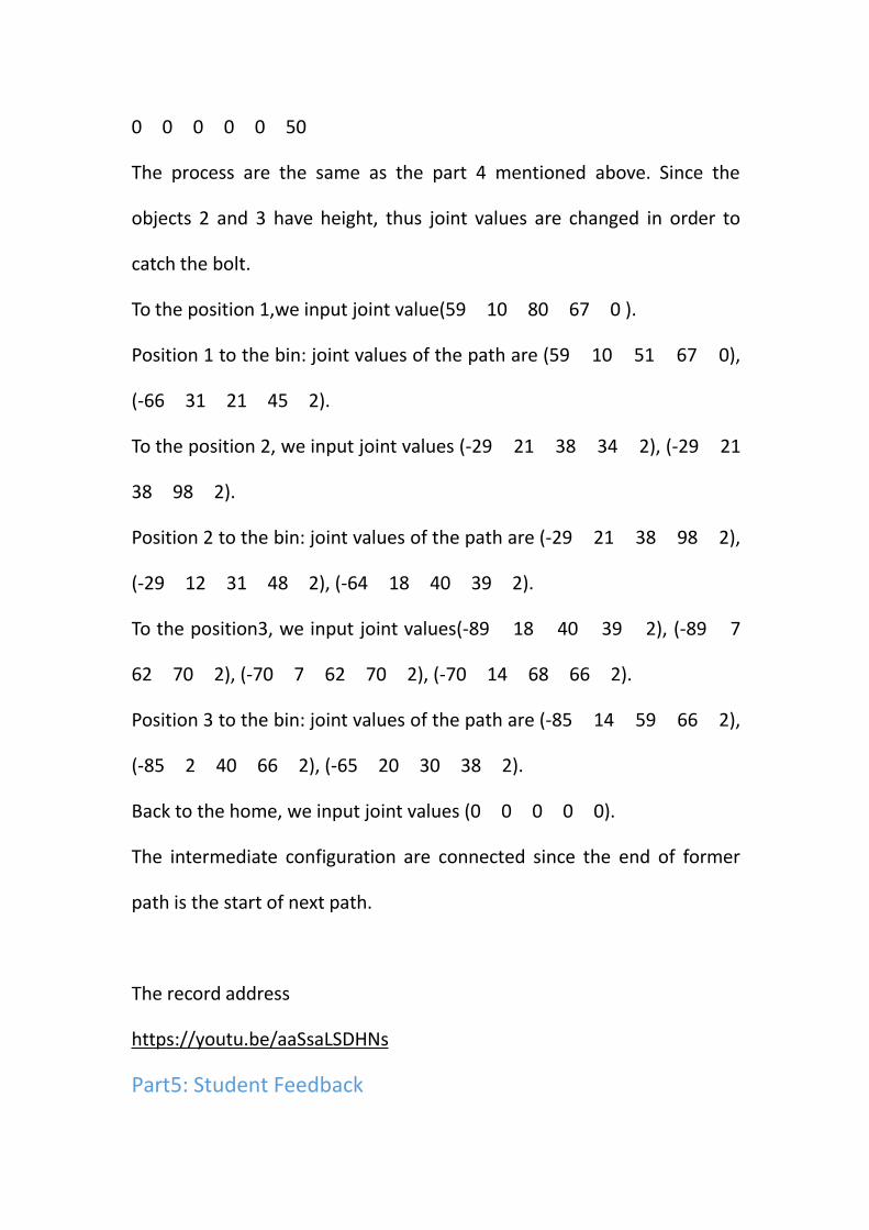
The process are the same as the part 4 mentioned above. Since the
objects 2 and 3 have height, thus joint values are changed in order to
catch the bolt.
To the position 1,we input joint value(59 10 80 67 0 ).
Position 1 to the bin: joint values of the path are (59 10 51 67 0),
(-66 31 21 45 2).
To the position 2, we input joint values (-29 21 38 34 2), (-29 21
38 98 2).
Position 2 to the bin: joint values of the path are (-29 21 38 98 2),
(-29 12 31 48 2), (-64 18 40 39 2).
To the position3, we input joint values(-89 18 40 39 2), (-89 7
62 70 2), (-70 7 62 70 2), (-70 14 68 66 2).
Position 3 to the bin: joint values of the path are (-85 14 59 66 2),
(-85 2 40 66 2), (-65 20 30 38 2).
Back to the home, we input joint values (0 0 0 0 0).
The intermediate configuration are connected since the end of former
path is the start of next path.
The record address
https://youtu.be/aaSsaLSDHNs
Part5: Student Feedback
We think that this lab is important for us to understand the robot motion
and control, we have tested the theory that we could plan the robot path
by inputting joint values calculated from inverse-kinematic equations.
We have taken two weeks to complete this exercise, and we
encountered some difficulties such as the ruler data is hard for us to read
exactly during measurement since the ruler is always tilted a little, and
the gripper was broken on our first robot arm so we needed to change
the machine and started all processes again. The biggest trouble we have
met is that we hardly to maintain same results for repeated processes
even every condition didn’t change, the bolt is also to hard to be caught
without dropping. Also, when we test our codes, we found that the
result was not correspond exactly o the statics of RAIS model.
The exercise could be improved if it sets more obstacles and complicated
goals for us to achieve because it could improve our skills much.
Appendix(MATLAB function code)
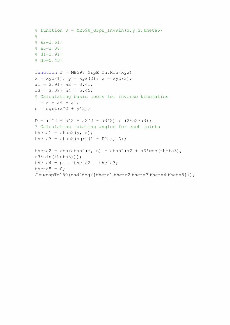
% function J = ME598_GrpE_InvKin(x,y,z,theta5)%% a2=3.61;% a3=3.08;% d1=2.91;% d5=5.45;
function J = ME598_GrpE_InvKin(xyz)x = xyz(1); y = xyz(2); z = xyz(3);a1 = 2.91; a2 = 3.61;a3 = 3.08; a4 = 5.45;% Calculating basic coefs for inverse kinematicsr = z + a4 - a1;s = sqrt(x^2 + y^2);
D = (r^2 + s^2 - a2^2 - a3^2) / (2*a2*a3);% Calculating rotating angles for each jointstheta1 = atan2(y, x);theta3 = atan2(sqrt(1 - D^2), D);
theta2 = abs(atan2(r, s) - atan2(a2 + a3*cos(theta3),a3*sin(theta3)));theta4 = pi - theta2 - theta3;theta5 = 0;J = wrapTo180(rad2deg([theta1 theta2 theta3 theta4 theta5]));


