'MEAN CROWDING' - britishecologicalsociety.org · Mean density, therefore, is misleading as a...

1

'MEAN CROWDING'

BY MONTE LLOYD*

Bureau of Animal Population, Department of Zoological Field Studies, Oxford University

The notion that animals in nature experience crowding is an inference from our own experience, a subjective idea, difficult to define and even harder to measure. Even so, there can be no doubt that the phenomenon exists; one can easily recognize some situations in which crowding must necessarily be greater than in others. By common sense, the degree of crowding that exists at any one moment must be a function, not only of the number of animals present in a given area, but also of their spatial pattern of distribution, their movements, their actions towards each other when they meet, and the physiological repercussions which these meetings bring about. For all we know, any of these things can influence any of the others, directly or indirectly, and the relationships may be different for different ages, sexes, different physiological conditions, and different local situations in the ever-changing habitat. To complicate the picture still more, animals can 'crowd' each other without ever meeting, by depleting some resource, or leaving traces, or making noises. The controversy about density-dependent factors which has engaged so much attention (Andrewartha 1957; Birch 1957; Nicholson 1957, 1958) is really an argument about the importance of crowding. How lamentable, therefore, that in most cases conclusions must be based on so crude a measure of crowding as 'mean density', the average number of individuals per unit of habitat.

This paper is concerned only with the first and easiest step towards a more sophisticated measure of crowding, namely taking into account the spatial pattern of microdistribution. As a further restriction, I am considering only freely moving animals that live in a relatively continuous habitat and do not defend territories (forest litter invertebrates, for example). Studies of territorial and sessile animals have always taken spatial relationships into account, needless to say. The study of spatial pattern has long been an important part of plant ecology (Grieg-Smith 1964), but here the concept of crowding is necessarily somewhat different, simply because the plants do not move about and 'encounter' one another. Many sea-shore invertebrates, though not sessile, tend to fill up their habitat as completely as plants do. No probability model based on dimensionless geometrical points could reasonably apply to such animals, and neither will the present treatment.

Animals that live in discrete ephemeral habitats (carrion, dung, decaying logs, kelp holdfasts, fungi, birds nests, etc.) present a different problem. A large proportion of these populations is often in transit, or searching, between suitable habitats, so it is generally impossible to devise sampling techniques that will catch resident and transient individuals with equal probability. The discussion to follow is not applicable to this situation either, unless one is content to draw conclusions that apply only to the resident section of the population.

We are restricting attention, then, to the case where knowledge of numbers and microdistribution is likely to be based on a series of randomly-placed quadrat samples in a continuous, apparently uniform habitat, and where the animals appear to be compara- tively rare. The pattern usually revealed is a curiously patchy one, the areas of high and

* Present address: Department of Zoology, University of California, Los Angeles, California 90024, U.S.A.

This content downloaded on Fri, 8 Mar 2013 13:49:31 PMAll use subject to JSTOR Terms and Conditions

http://www.jstor.org/page/info/about/policies/terms.jsp

2 'Mean crowding'

low local density not corresponding to any obvious differences in habitat. In such a distribution, the majority of individuals find themselves in a local patch of relatively high density, in close proximity to many more individuals of their own kind than would be the case, on the average, if the distribution were random. In this sense, a typical individual is more 'crowded' than it would be in a random distribution having the same mean density. Mean density, therefore, is misleading as a measure of crowding. What is needed is a measure, not of mean number per quadrat, but mean number per individual.

An imaginary circle drawn around each individual might include from none to several others like it-other individuals that may be (or may recently have been, or may soon be) exerting some kind of crowding effect on the one at the centre. The most appropriate size to make this circle, i.e. the 'ambit' of a typical individual, would of course have to be determined empirically for each species. If that were done, and if the exact instantaneous spatial distribution were completely known, one could take the number of other individuals momentarily within its ambit as a measure of the crowding currently being exerted on each individual. Averaging this over all individuals in a population yields a parameter that I will call 'mean crowding'-remembering that a great deal more than spatial distribution will ultimately have to be taken into account before one can pretend to have an ecologically realistic measure of crowding. 'Mean crowding', as presently defined, is merely the obverse of Thompson's (1956) mean distance to the nth nearest neighbour; I wish instead to measure the mean number of neighbours within a certain distance D = (a/ir)I, where a is the average ambit of an individual.

With the data in the form of quadrat counts, one's information on spatial distribution is incomplete. A measure of 'mean crowding' can still be got, however, if one assumes that the positions of the animals are random with respect to each other and constantly changing. The other individuals momentarily within the imaginary circle are regarded as a kind of influence 'smeared' uniformly over space, the extent of this influence being about the same just outside the circle as within it. In other words, if quadrat size coincides reasonably well with the size of the individual's ambit, then the scale of the patchiness should be large compared with quadrat size. This being so, the number of other animals momentarily in the same quadrat as a given individual provides a good estimate of the number of others in a circle centred on it, having the same area. 'Mean crowding', then, can be measured by the mean number per individual of other individuals in the same quadrat. One might choose to be interested in this quantity, of course, even though the organisms were sessile. There is no mathematical reason to restrict attention to moving animals with respect to 'mean crowding', but I think it makes much better ecological sense to do so.

In the following pages, I will first consider 'mean crowding' in the unusual situation where quadrat information is complete, i.e. where all quadrats in the area of study have been censused. Secondly, estimates of 'mean crowding' and standard errors are given for sample data. Thirdly, I will discuss possible applications as an ecological tool, in the light of implicit assumptions, in the interpretation of rare species, the effect of quadrat size, and the search for evidence concerning population-governing mechanisms. Finally, two obvious extensions are briefly mentioned, one to deal with 'mean crowding' on one species by another, and another to define 'subjective' species diversity.

NUMERICAL ILLUSTRATION WITH COMPLETELY KNOWN PARAMETERS

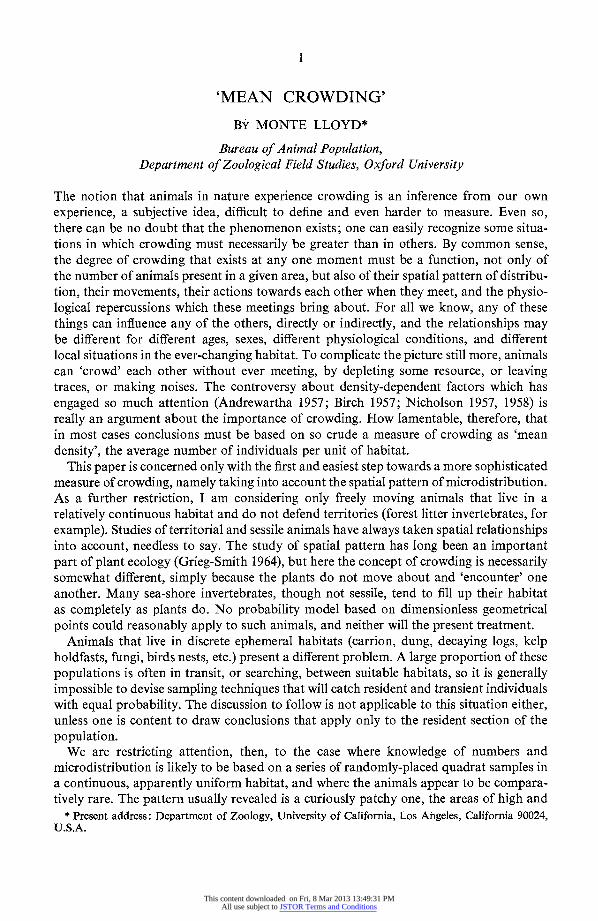
Consider the data for Lithobius crassipes L. Koch shown in Fig. 1 and imagine, merely for purposes of illustration, that the surrounding region is of no interest, i.e. that these



MONTE LLOYD 3

Q = 37 quadrats make up the whole area of study. The 'sample' is therefore a complete one; true values of mean and variance are exactly known. Starting with the top row of hexagons, working from left to right, we read xj, the number present in each quadrat- xj: 0,2,0,0; 1,0,2,0,2;0,0,0,0,0,2;0,2,0,1,1,1,2; 1,1,0,0,3,1;0,3,1,2,0; 1,0,1,0 (j= 1,2,... Q 37). The sum, sum of squares, mean density (m), and variance (a2) are:

Q Q Exj= N = 30 Ex = 56

i= j-

QN 30 m = xj = Q = T7 = 0 811 individuals per quadrat (1)

j ~Q

= X -( QXj)2/Q 56-900/37 0856 (2)

Q 37

So much is ordinary, standard statistics. Now we write down, for each of the N = 30 individuals, the number of other indivi-

duals that are located with it in the same quadrat. Call these numbers Xi. Taking the

2 2 00 3 12 0

3 f t

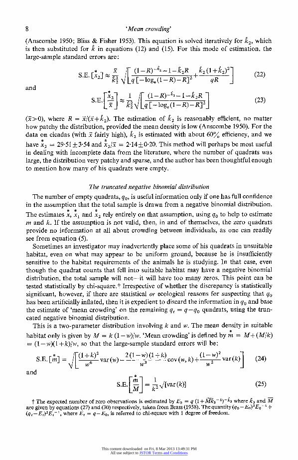
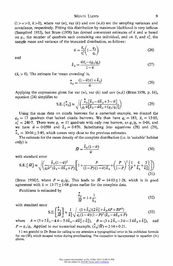
FIG. 1. The numbers of Lithobius crassipes collected in thirty-seven contiguous hexagonal quadrats of beech litter at Wytham Woods, near Oxford, on 30 October 1958. The quadrats are 1 ft (0 30 m) across, so the total area sampled is about 6 ft from side to side. Individual

quadrats have an area of 0 866 ft2 (0-08 m2); the distribution is locally random.

quadrats in the same order as before, we have Xi: 1,1;0,1,1,1,1 ;1,1;1,1,0,0,0,1,1;0,0,2,2, 2,0;2,2,2,0,1,1 ;0,0 (i = 1,2,..., N = 30). The 'mean crowding' (m) is,

N

Xi 26 ml =0N = = 0867 other individuals per quadrat per individual. (3)

Equation (3) emphasizes that m* is a mean, averaged over individuals rather than quadrats. Unlike m, m* is not affected by the empty quadrats, which provide no information about individuals.



4 'Mean crowding'

For calculation, it is more convenient to express m directly in terms of the numbers in each quadrat, the xjS. Because of the identity,

N Q

E Xi= Lixj(xj-l) (4) j=

we have Q

* x

56 m j - 1 - 1 = --I = 0 867 other individuals per quadrat per individual. (5) Q

~~30 j = 1

Substituting equations (1) and (2) into equation (5) yields the relationship between mn and m;

2

mn = m+ --1) (6) m

In other words, the amount by which the ratio of variance to mean density exceeds unity, added to the mean density itself, gives the 'mean crowding'. In a random distribution, of course, the variance and mean density are equal, so the quantity in parentheses

disappears, and mi and m are equal. This situation is well-represented by the data in Fig. 1, which are statistically indistinguishable from a random distribution.

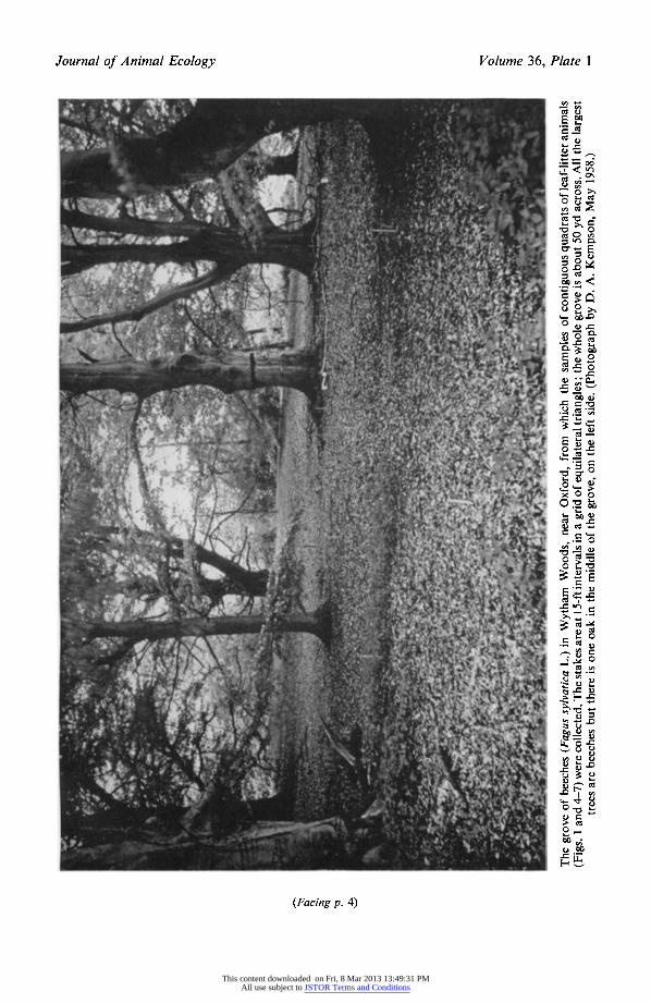
Plate 1 is a photograph of the small grove of beech trees from which the samples in Fig. 1 were collected. The whole grove is only about 50 yd across, and hence has about 500 times the area shown in Fig. 1. From other sampling, it is clear that if this area could have been completely censused, then patches of higher and lower density would have become evident. For example, a series of six short transects was collected on 3-6 July 1958, from beech litter near the periphery of the grove. Each transect consisted of six quadrats the size and shape of those in Fig. 1, but taken at 2-ft intervals, each line of quadrats oriented at random in one of three compass directions. The following numbers of L. crassipes were found:

Transect A: 9, 7, 5, 4, 1, 0 Transect B: 0, 0, 0, 0, 1, 0 Transect C: 3, 1, 5, 3, 3, 1 Transect D: 0, 1, 2, 4, 2, 0 Transect E: 0, 0, 0, 0, 1, 1 Transect F: 2, 1, 2, 4, 5, 10

If the L. crassipes occupying the litter under this one grove of beeches (Plate 1) can be considered one population, then it is clear that the 'mean crowding' for the population as a whole considerably exceeds its mean density, even though the distribution in a given local area appears to be random. Statistical estimates of 'mean crowding' and mean density for the grove as a whole would of course require data from a large number of randomly placed quadrats collected simultaneously. I did not try to count that many quadrats in this particular case.

SAMPLE ESTIMATES

In most ecological studies based on random quadrat sampling, the sampled quadrats will form a small part of the whole area of study. The true mean density, m, will be



!'SSI * i - ' t-X: _ E ':t . ' == '_~~~~~~~~~~~~~~~~~~~~~~~~~~~~~~~~~~~~~~~~~~~~~~~~~~~~~~~-

nD * w! Sl~~~~~~~~~~~~~~~~

4 4 a! 11 ma~~~~~~~~~~~~~~~~~~~~~~~~~~~~~~~I5 Th roeofbece (au s/atc L)inWtamWod,nerOxod fo wih h smle fcotguu qaraso la-lteraiml

(Figs. I and F7) were collected. The stakes are at 1 5-ft intervals in a grid of equilateral triangles; the whole grove is about 50 yd across. All the largest vo~~~~~~~~~~~~~~~~~~~~~~~~~~~~~~~~~~~~~~~~~~~~~~~~~~~~~~~~~~~~~~~~~~~~~~~.. .... tree ar beche bu thre s oe ok i th midleof he rov, o th let sde.(Phtogaphby . A Kepso, My 158.



MONTE LLOYD 5

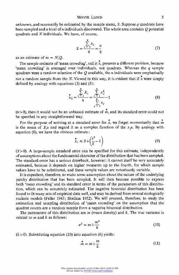
unknown, and necessarily be estimated by the sample mean, x. Suppose q quadrats have been sampled and a total of n individuals discovered. The whole area contains Q potential quadrats and N individuals. We have, of course,

zxj n

q q

as an estimate of m = N/Q.

The sample estimate of 'mean crowding', call it x, presents a different problem, because 'mean crowding' is averaged over individuals, not quadrats. Whereas the q sample quadrats were a random selection of the Q available, the n individuals were emphatically

not a random sample from the N. Viewed in this way, it is evident that if I were simply defined by analogy with equations (3) and (5):

n q

Exi EX-i xo= n = q 1 (8)

E xj j = I

(n > 0), then it would not be an unbiased estimate of mi, and its standard error could not be specified in any straightforward way.

For the purpose of arriving at a standard error for x, we forget momentarily that m is the mean of Xis and regard it as a complex function bof the xjs. By analogy with equation (6), we have the obvious estimate:

XI +(9)

(x>0). A large-sample standard error can be specified for this estimate, independently of assumptions about the fundamental character of the distribution that has been sampled. The standard error has a serious drawback, however: it cannot itself be very accurately estimated, because it depends on higher moments up to the fourth, for which sample values have to be substituted, and these sample values are notoriously variable.

It is expedient, therefore, to make some assumption about the nature of the underlying patchy distribution that has been sampled. It will then become possible to express both 'mean crowding' and its standard error in terms of the parameters of this distribution, which can be accurately estimated. The negative binomial distribution has been found to fit many sets of empirical data well, and may be derived from several ecologically realistic models (Feller 1943; Skellam 1952). We will proceed, therefore, to study the estimation and sampling distribution of 'mean crowding' on the assumption that the quadrat counts are a random sample from a negative binomial distribution.

The parameters of this distribution are m (mean density) and k. The true variance is related to m and k as follows:

a2 = m + k (10)

(k>O). Substituting equation (10) into equation (6) yields:

m= m+ (11) m =m k



6 'Mean crowding'

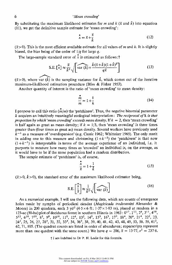
By substituting the maximum likelihood estimates for m and k (x and k) into equation (11), we get the definitive sample estimate for 'mean crowding':

x = 5x+g k(12)

(x > 0). This is the most efficient available estimate for all values of m and k. It is slightly biased, the bias being of the order of 1 /q for large q.

The large-sample standard error of x is estimated as follows:t

S.E. [x] l: T [var( l+ (x+(k2jl+)) (13)

(x>O), where var (k) is the sampling variance for k, which comes out of the iterative maximum-likelihood estimation procedure (Bliss & Fisher 1953).

Another quantity of interest is the ratio of 'mean crowding' to mean density:

-= 1 +- (14) m k

I propose to call this ratio ( m*/m) the 'patchiness'. Thus, the negative binomial parameter k acquires an intuitively meaningful ecological interpretation: The reciprocal of k is that proportion by which 'mean crowding' exceeds mean density. If k = 2, then 'mean crowding' is half again as great as mean density; if k = 1/3, then 'mean crowding' is three times greater than (four times as great as) mean density. Several workers have previously used k-' as a measure of 'overdispersion' (e.g. Cassie 1962; Whittaker 1965). The only merit in adding one to this measure and christening (1 +k-') the 'patchiness' is that now (1 + k-) is interpretable in terms of the average experience of an individual, i.e. it purports to measure how many times as 'crowded' an individual is, on the average, as it would have to be if the same population had a random distribution.

The sample estimate of 'patchiness' is, of course,

x 1 -= =1J+- (15) x ki

(x>0, k>0), the standard error of the maximum likelihood estimator being,

S [x 1 J[ (16) S.E. -11.

k2 var (1?)]

As a numerical example, I will use the following data, which are counts of emergence holes made by nymphs of periodical cicadas (Magicicada tredecassini Alexander & Moore) in 200 quadrats, each 3 yd2 (4-5 x 6 ft; 1-37 x 1-83 m), placed at random in a 123-ac (50-ha) plot of deciduous forest in southern Illinois in 1963: 0'7, 1"l, 28, 311, 410, 512, 610, 710, 85, 99, 1010, 118, 124, 132, 145, 159, 165, 175, 184, 204, 214, 222, 23, 243, 25, 26, 27, 283, 31, 32, 333, 34, 363, 38, 39, 40, 41, 42, 43, 48, 49, 53, 58, 59, 612, 62, 71, 105. (The quadrat counts are listed in order of abundance; superscripts represent more than one quadrat with the same count.) We have q = 200, - = 13 77, s2 = 237-8.

t I am indebted to Dr P. H. Leslie for this formula.



MONTE LLOYD 7

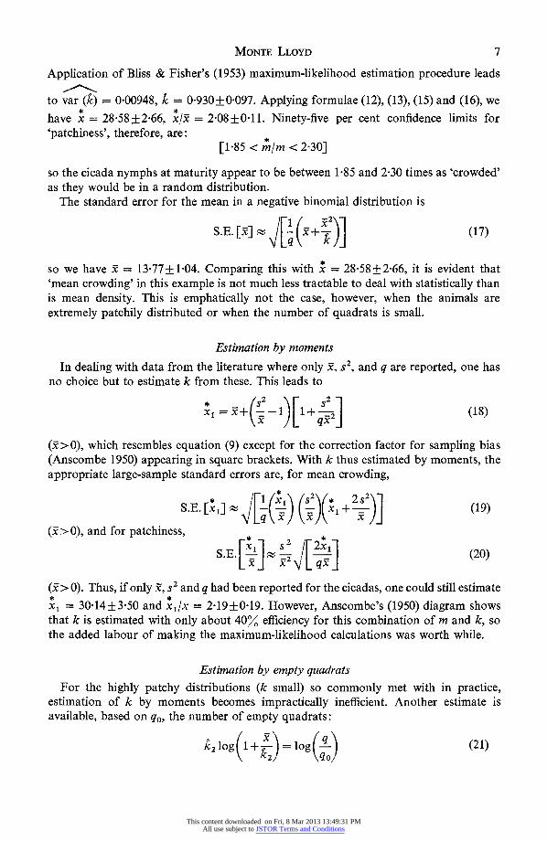
Application of Bliss & Fisher's (1953) maximum-likelihood estimation procedure leads

to var (k) = 000948, 1 = 0930+0 097. Applying formulae (12), (13), (15) and (16), we **

have x = 2858+2 66, x/x = 2-08+0011. Ninety-five per cent confidence limits for 'patchiness', therefore, are:

[1.85 < m/m < 2 30]

so the cicada nymphs at maturity appear to be between 1 85 and 2-30 times as 'crowded' as they would be in a random distribution.

The standard error for the mean in a negative binomial distribution is

S.[l E. [9 )] (17) so we have x = 13-77+1-04. Comparing this with x = 28 58+2 66, it is evident that 'mean crowding' in this example is not much less tractable to deal with statistically than is mean density. This is emphatically not the case, however, when the animals are extremely patchily distributed or when the number of quadrats is small.

Estimation by moments

In dealing with data from the literature where only x, s2, and q are reported, one has no choice but to estimate k from these. This leads to

I (s )[ s2 1 (18)

(9>0), which resembles equation (9) except for the correction factor for sampling bias (Anscombe 1950) appearing in square brackets. With k thus estimated by moments, the appropriate large-sample standard errors are, for mean crowding,

S.E. [X JQ] +') (x)( xj)] (19)

(9>0), and for patchiness, *2*

S.E. [X] s2|- W3 j ~(20)

(x > 0). Thus, if only , s2 and q had been reported for the cicadas, one could still estimate T T

xil=-30'14+3'50 and xi/x = 2-19+0-19. However, Anscombe's (1950) diagram shows that k is estimated with only about 4000 efficiency for this combination of m and k, so the added labour of making the maximum-likelihood calculations was worth while.

Estimation by empty quadrats For the highly patchy distributions (k small) so commonly met with in practice,

estimation of k by moments becomes impractically inefficient. Another estimate is available, based on qo, the number of empty quadrats:

k2 lg109 )= log(-) (21)



8 'Mean crowding'

(Anscombe 1950; Bliss & Fisher 1953). This equation is solved iteratively for k2, which is then substituted for k in equations (12) and (15). For this mode of estimation, the large-sample standard errors are:

( R [-( Rk21I- 2R k2(1+k2)1 (22)

2 ( - ) -R]~+' qR j and

S.E. X2 - 1 (1-R)A-1-k2R ~~~(23)

[ 22 1q[lg (l-R)-R] ](3

(Q >0), where R = 5-/( + 22). The estimation of k2 is reasonably efficient, no matter how patchy the distribution, provided the mean density is low (Anscombe 1950). For the data on cicadas (with x fairly high), k2 is estimated with about 60%. efficiency, and we

have X2= 29-51 +354 and X2/X = 2-14+0-20. This method will perhaps be most useful in dealing with incomplete data from the literature, where the number of quadrats was large, the distribution very patchy and sparse, and the author has been thoughtful enough to mention how many of his quadrats were empty.

The truncated negative binomial distribution

The number of empty quadrats, qo, is useful information only if one has full confidence in the assumption that the total sample is drawn from a negative binomial distribution.

* * *

The estimates x, xl and x2 rely entirely on that assumption, using qo to help to estimate m and k. If the assumption is not valid, then, in and of themselves, the zero quadrats provide no information at all about crowding between individuals, as one can readily see from equation (5).

Sometimes an investigator may inadvertently place some of his quadrats in unsuitable habitat, even on what may appear to be uniform ground, because he is insufficiently sensitive to the habitat requirements of the animals he is studying. In that case, even though the quadrat counts that fell into suitable habitat may have a negative binomial distribution, the total sample will not-it will have too many zeros. This point can be tested statistically by chi-square.t Irrespective of whether the discrepancy is statistically significant, however, if there are statistical or ecological reasons for suspecting that qo has been artificially inflated, then it is expedient to discard the information in qO and base the estimate of 'mean crowding' on the remaining qt = q-qo quadrats, using the truncated negative binomial distribution.

This is a two-parameter distribution involving k and w. The mean density in suitable

habitat only is given by M = k (1- w)/w. 'Mean crowding' is defined by m = M+ (Mlk) (1 - w)(1 + k)/w, so that the large-sample standard errors will be:

S.E. = [(1+ k)2 2 (1- w) (1+ k) ~k+w ] (4 S.E. [m] 4 /[( + k)var (w) - -

3 cov (w, k) + 2 var (k) (24)

and

S.E.[j = A-V[var(k)] (25)

t The expected number of zero observations is estimated by Eo = q (1 + Mfc3 - 1)-k3 where k3 and M are given by equations (27) and (30) respectively, taken from Brass (1958). The quantity (qo -Eo)2Eo- + (q,-EE)2E,- , where E, = q-Eo, is referred to chi-square with 1 degree of freedom.



MONTE LLOYD 9

(1> w >0, k> 0), where var (w), var (k) and cov (w,k) are the sampling variances and covariance, respectively. Fitting this distribution by maximum likelihood is very tedious (Sampford 1955), but Brass (1958) has devised convenient estimates of k and w based on ql, the number of quadrats each containing one individual, and on x- and s2, the sample mean and variance of the truncated distribution, as follows:

w= 2 - (26) St qt

and

3 i-(/ (27)

(5t > 0). The estimate for 'mean crowding' is,

=(1-f)(1+/3) (28)

Applying the expressions given for var (w), var (k) and cov (w,k) (Brass 1958, p. 61), equation (24) simplifies to

S.E. [X3] r|( q3:;ii2 /] ) (29)

Using the same data on cicada burrows for a numerical example, we discard the qo= 17 quadrats that lacked cicada burrows. We then have qt = 183, it = 15-05,

s2= 240-7. There were q= 11 quadrats with only one burrow, so qllqt = 006, and we have wi = 0O0588 and k3 = 0876. Substituting into equations (28) and (29),

X3 = 3004 + 3 45, which comes very close to the previous estimates. The estimate for the mean density of the complete distribution (i.e. in 'suitable' habitat

only) is M= 23(1- (30)

w

with standard error

( (I _1 ii^)2 p2_ S.E. FRI /-% I3(

W)+ P+ ( ) { + ~ 4- +3}]

(31)

(Brass 1958)t, where P = qi/qt. This leads to M = 14-03+1-28, which is in good agreement with 5x = 13-77+ 1 04 given earlier for the complete data.

Patchiness is estimated by *

X3 = 1 +- (32) M 3

with standard error

[x] 1 /(1 +k) (2 k3+k3AP +Bp2) S E [3 t 2 qt (1- w) (I _ p)2 (k3 _ W^k3 + P)

where A = (5 + 2 23-4 w k _k +k B = (3+2k 3-3 w-3*3 w + k2), and P = ql/qt. Applied to our numerical example, (x/3M) =2-14+0 21.

t I am grateful to Dr Brass for calling to my attention a typographical error in his published formula for var (M), which escaped notice during proofreading. The correction is incorporated in equation (31) above.



10 'Mean crowding'

'Mean demand'

The index x is taken as the mean number of other individuals per quadrat per individual, on the assumption that an animal does not 'crowd' itself. If the crowding operates, not by hostile encounters between individuals, but through depletion of some expendable resource, then obviously an individual does 'crowd' itself, in the sense that it may eat today what it could otherwise have had tomorrow. This suggests another index, the mean number of individuals per quadrat per individual. To avoid confusion, I will call this the

'mean demand', but no new symbol is required for it, since it is always simply (x +1),

with of course the same standard error as for x. For the 'complete' data in Fig. 1, the

'mean deinand' is (m + 1) = 1 87. This says that the average centipede (Lithobius crassipes) in this small area lives in a quadrat in which there are 1*87 mouths to feed, including its own, and excluding competing species.

If one has data for each quadrat that relate to the rate of supply of the expendable resource, say rj (j = 1,2, . . .,Q), one can incorporate these into a measure of 'mean demand relative to local supply', which might be different from the 'mean demand' per quadrat being made on the resources of the area as a whole. One possible formula would be

Qt

Zx2lrh h 1 ~~~~~~~~(34) Qt ct

Qt E xh |E rh hx= I/ h =

(Yx > 0), applied to the truncated distribution, with quadrats renumbered (h = 1,2,.. ., Qt). For the extreme case where all of the patchiness is explainable by resource availability

(i.e. Xh = crh, with c constant), the above reduces to ( + 1) = mt, where mt is the mean of the Qt occupied quadrats. There are various other formulae that could be argued for as well, but standard errors for sample estimates are not available for any of them. This would require a sampling theory for contagious distributions in which quadrat 'size' is not constant. So far as I am aware, this has not yet been developed.

ASSUMPTIONS AND APPLICATIONS

Looking at equation (6), one can interpret the 'mean crowding' of a patchily-distributed population as that mean density which the population could have, and be no more crowded on the average than it is now, if it had a random distribution. According to this view, mean density and patchiness are interconvertible. Any two populations are considered equivalent, in respect of the biological effects of crowding, if they have the same 'mean crowding', i.e. the same product of mean density and 'patchiness'. Stated in this way, one of the implicit assumptions becomes evident: that the effects of crowding vary linearly with the number of local crowders-an individual will be exactly twice as affected by ten others around it, for example, as it would be by five others. This may be true over a wide range of crowding, but biparental species must have some optimum degree of local crowding, below which reproduction is hampered because many females go unfertilized.

Indeed, it might be argued that patchy distributions probably have much more to do with 'undercrowding' than with deleterious overcrowding. The only unequivocal evidence for crowding that can come from an instantaneous pattern of microdistribution appears when the distribution is more regular than random (a'2 < m), suggesting that the presence



MONTE LLOYD 11

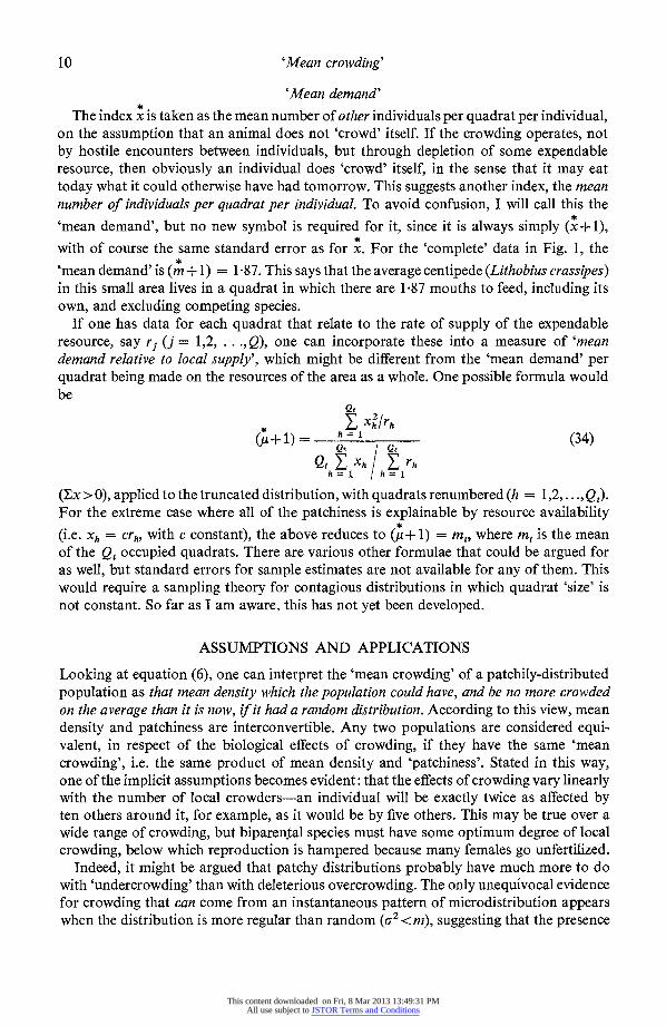
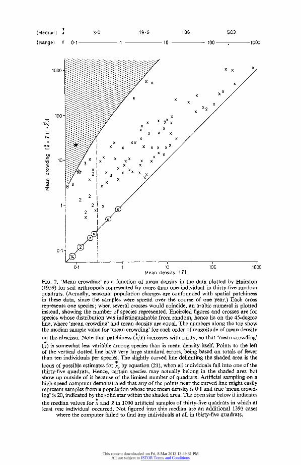
of certain individuals has prevented others from settling nearby. When distributions are patchy (cr2 > m), there is a marked tendency, among different species of comparable size and ecology, for the rarer species to be the more patchily distributed (Hairston 1959).t As a result, 'mean crowding', though very far from being a universal constant, tends to be considerably less variable among species than is mean density itself.

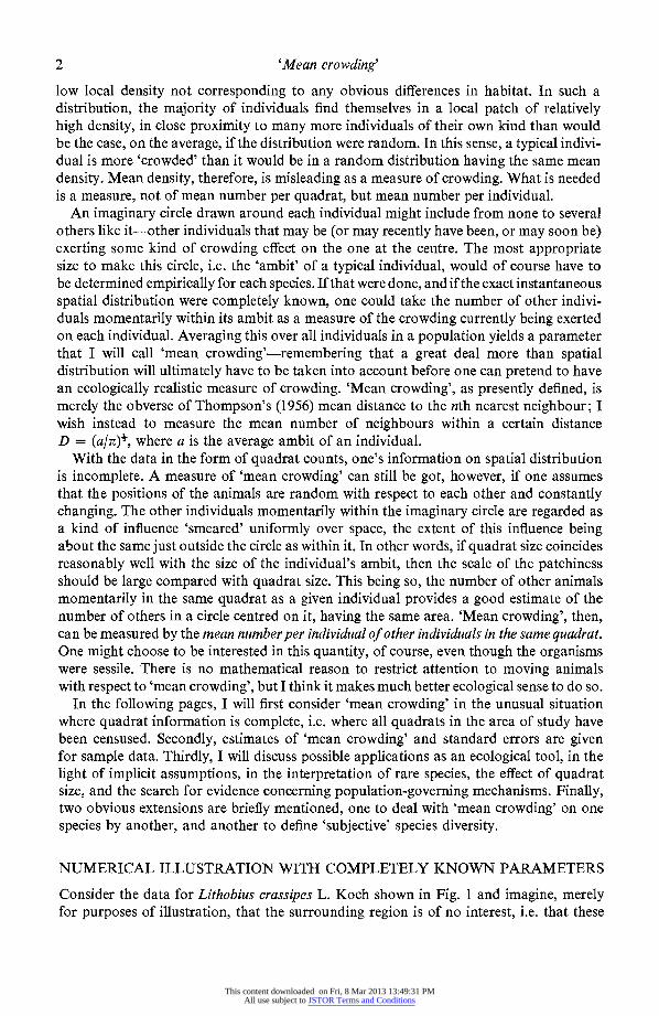
This is shown in Fig. 2 by replotting Hairston's Fig. 1 as x = x(l + k'- ) versus x, both on logarithmic scales. Mean density (for thirty-five quadrats) varies over roughly four orders of magnitude, i.e. from 0-1 to 1000 per ft2, while the median values for 'mean crowding' in each density bracket go from x = 3 0 when 0 I < x < 1 to x = 503 when 100 <5< 1000. Such an effect could be interpreted to mean that individuals have the least tendency to wander when they are in the vicinity of some optimum number of others of their own species, and that perhaps this optimum number is broadly similar in different species.

Hairston (1959) interprets his data in a different way, one that does not necessarily *

assume any constancy in m. He simply assumes that large parts of the area sampled are not suitable habitat for the rarer species, that they are, in fact, rare for this very reason, and so automatically appear to be more patchily distributed. Feller (1943) showed that one cannot tell, from the frequency distribution alone, which of these two hypotheses is correct.

Rare species: severe sampling problems

Rare patchy species will often be missed altogether by the sampling, or, even if found, will not always be recognizably patchy unless the number of quadrats is very large. It cannot be emphasized too strongly that formulae for standard errors given in the previous section have as a prior condition that the species has actually been found in the sample (5 > 0). The species about which one draws inferences should be specified a priori. If one simply lays out a set of random quadrats and takes the species as they come (as one might do in a study of species diversity), then no conclusions can be drawn about any species so patchy or rare that one was not assured a priori of encountering it with q quadrats.

As Anscombe (1950) points out, no matter how many quadrats one sets out to sample, there is always a chance that the species of interest will fail to occur in any of them. Hence, it is not possible, strictly speaking, to give a standard error for k in the negative binomial, and the same applies to 'mean crowding' and 'patchiness'. Even x is not an unbiased estimator of m, unless the species in question has been named a priori. The mere fact that one has encountered an (unexpected) rare species in a small series of quadrats means

t After writing the above, I read Taylor's (1961) paper in which he finds that empirical data fit a 'power law' relating variance to mean: o2 = amfl. He concludes: 'This implies that populations aggregated at high density tend to become regular when density diminishes, and vice versa . . .'. The apparent contradiction to the findings of Hairston and others disappears when one realizes that Taylor is using

m as a measure of patchiness. For 8> 1, the 'power law' does indeed imply that a2/m = aM- 1 decreases steadily with decreasing mean. However, the same law also implies that 'patchiness' as defined by m = (m+cr2m 1-1)/r = am$2-m' +1 will be increasing with decreasing mean-provided that 2>,/5> 1 and a> ~ '). Most of the published examples cited by Taylor fall within this range; in those that do not, there is no strong relation between 'patchiness' and rarity, either way. I conclude, in agreement with Evans (1952) and Morisita (1962), that a2lm is not a good measure of the degree of patchiness-in fact, it is downright misleading-even though x2 (q- 1)a2/m is the standard statistical test for patchiness, and a good one. (None of this has any critical bearing on the main concern of Taylor's paper, which is to find a family of transformations that will render data from quadrat counts amenable to conventional statistical analysis.)



(Median) x 3 0 19 5 106 503

(Range) i 01 1 10 100 1000

1000~ ~ ~ ~~~~~Ma dest ( X )

X X ~~XX

X2

100

FIG. 2. 'Mean crowding' as a function of mean density in the data plotted by Hairston (1959) for soil arthropods represented by more than one individual in thirty-five random quadrats. (Actually, seasonal population changes are confounded with spatial patchiness in these data, since the samples were spread over the course of one year.) Each cross represents one species; when several crosses would coincide, an arabic numeral is plotted instead, showing the number of species represented. Encircled figures and crosses are for species whose distribution was indistinguishable from random, hence lie on the 45-degree line, where 'mean crowding' and mean density are equal. The numbers along the top show the median sample value for 'mean crowding' for each order of magnitude of mean density on the abscissa. Note that patchiness (x/x) increases with rarity, so that 'mean crowding'

(x~) is somewhat less variable among species than is mean density itself. Points to the left of the vertical dotted line have very large standard errors, being based on totals of fewer than ten individuals per species. The slightly curved line delimiting the shaded area is the locus of possible estimates for x, by equation (21), when all individuals fall into one of the thirty-five quadrats. Hence, certain species may actually belong in the shaded area but show up outside of it because of the limited number of quadrats. Artificial sampling on a high-speed computer demonstrated that any of the points near the curved line might easily represent samples from a population whose true mean density is 0 1 and true 'mean crowding' is 20, indicated by the solid star within the shaded area. The open star below it indicates the median values for x and x in 1000 artificial samples of thirty-five quadrats in which at least one individual occurred. Not figured into this median are an additional 1393 cases

where the computer failed to find any individuals at all in thirty-five quadrats.



MONTE LLOYD 13

there is a better than even chance that this species is still rarer than its sample mean indicates.

To give myself some first-hand experience of these sampling difficulties, I programmed the IBM 7094 computer at the University of California, Los Angeles, to generate the full negative binomial distribution for which m- 01 and m = 20 (indicated by the star within the shaded area in Fig. 2). This is about the 'mean crowding' typical in Hairston's data for species with mean densities between 1 and 10. Then, with a random number table, I sampled from this distribution, thirty-five quadrats at a time, for different hypothetical 'species', until 100 'visible species' (present in at least one quadrat) had been found. I was expecting the results to be erratic, but I was unprepared for the extremes that actually obtained. Seventy-five of the 100 species were found only in one quadrat, ranging from a single individual (twenty-four cases) up to one instance with eighty-four in one quadrat: 124 - 27 - 38 _ 44 59 - 62 - 72 - 8 _ 92 103 - 122 - 14 - 192 -24 -26 -

29 - 35 -43 - 55 - 80 - 84 (superscripts indicate number of species). One species was represented in five of the thirty-five quadrats: (1,1,2,4,21); the remaining twenty-four species were each found in two quadrats only: (1,1)2-(1,3)4-(2,4)_(1,7)2-(4,5)- (1,9) - (1,10) - (2,13) - (7,8) - (3,13)2 - (2,16) - (6,13) - (9,13) - (3,20) - (6,19) - (12,18) - (7,28) - (13,24). Sample mean densities range from x = 0 03 up to x = 2-4, with mean 429 and median 0-14. In addition to the 100 'visible species', another 167 species were

completely missed by the sampling. When these are figured in, the mean x is 0 1 1, close to the true value m = 0-10.

Table 1. Numbers of random quadrats needed to discover a species in at least one quadrat (with 9900 assurance) when the distribution is negative

binomial with mean density (m) and patchiness (im/m) as shown Mean density Patchiness (mrnrm) = (1 +k- 1)

(in) 2 20 200 2000

1.0 7 29 173 1211 0.1 48 82 301 1736 0 01 463 503 858 3024

Sample values for 'mean crowding' (from equations 21 and 12) have an enormously skewed distribution, ranging all the way from x = 0-03 to I = 524, with median 9'2 and mean 35-2 (compare with true value m= 20). An additional 1000 samples of thirty-five quadrats each were taken from the computer at a later time, yielding a median x of 5-6. Upper and lower quartiles were 26-0 and 0-06 respectively; octiles were 54-7 and 0'03. A quarter of the samples (25.90 ) consist of one or two isolated individuals-indistinguishable from a random distribution with very low mean. The distortion expected from a 'typical' (median) sample is illustrated in Fig. 2, although relatively few samples lie

*

anywhere near the medians for x and x. As a practical procedure, it is expedient to set up some minimum number of quadrats,

4, for species of a given rarity (m) and patchiness (1 + k-), such that, if q <q, one avoids drawing any conclusions at all. For the negative binomial, the number of quadrats necessary to insure with 9900 probability that a given species will occur at least once in the sample is given implicitly by 1- (1 +mk- 1)-kq - 0.99. Explicitly,

q = log (100)/k log (1 + mk-1) (35)

B J.A.E.



14 'Mean crowding'

This function is illustrated in Table 1 for several combinations of mean density and

patchiness. For m = 0-10 and m = 20 (mA/m = 200), Table 1 calls for at least 301 quadrats. When applied to a particular unexpected rare species, Table 1 gives somewhat less than the 9900 assurance it claims, because one must substitute into equation (35) the sample estimates k and x, which are biased and likely to be wide of the mark for a patchy

rare species. Even when q> q, the standard error for x can be prohibitively large.

Rare species: ecological interpretation

One would think an exceedingly rare (biparental) species must necessarily be exceedingly patchy-or exceedingly vagile-if its members are to have enough experience of one another to function as a population. One might postulate that those species whose true 'mean crowding' falls below a certain critical minimum are 'refugees' from elsewhere. Terrestrial ecosystems tend generally to be complex mosaics of interspersed habitats (Watt 1947; Elton 1949). Every species must have a 'headquarters' in one or another of these habitats (Paviour-Smith 1960), and produce a population excess there, if that species is to persist in the ecosystem as a whole. Some of the excess presumably falls prey to resident predators or other local hazards, but much of it must often emigrate to other nearby habitats, if the species have any vagility at all (e.g. see Johnson, Taylor & South- wood 1962).

In a given habitat at any moment, then, one should expect to be able to find two kinds of rare species-those that 'belong' and those that do not, i.e. those that maintain populations there (however local these populations may be) and those that are 'subsidized' from elsewhere. It follows that a frequency distribution of 'mean crowding' for rare species should be distinctly bimodal. Potentially, this might be a useful criterion for eliminating from consideration the 'refugee' species, say, in a study of species diversity. To get adequate data, however, one requires many hundreds of quadrats (see Table 1). Also, judgment must be suspended on samples consisting of one or two isolated individuals, because this result can come as easily from a rare patchy distribution as from a rare random one.

If one could measure the 'ambit' of each species (a), one would expect xa to be even

less variable than x. Perhaps some of the variability in x shown in Fig. 2 could be explained in this way, if the commoner species (perhaps tending to be smaller) tend to have smaller ambits. In the case where different quadrat sizes, 0, have been used for sampling different

species, one would of course calculate xa/O to place comparisons on a common scale.

Quadrat size

The natural choice for quadrat size (0) is the average ambit of an individual (a), as suggested earlier. Ambit is not an easy parameter to measure for most species in nature. Berthet (1964) has made important progress by showing that one can follow the movements through leaf litter of animals even so small as mites, by tagging them radioactively. A suitably rigorous definition for an 'ambit' is not self-evident, however, even when one has such data available. There is much that might be borrowed from the extensive work on home range in mammals (Blair 1940; Stickel 1946; Hayne 1949, 1950; Dice & Clark 1953; Godfrey 1954; Calhoun & Casby 1958; Brant 1962) but no attempt will be made here to develop this subject further. In practice, I think the issue of suitable quadrat size need not be a serious stumbling block because, within certain limits, one can use any



MONTE LLOYD 15

convenient quadrat size and reduce to standard measure. That is to say, x/O should be independent of quadrat size over a fairly wide range of quadrat sizes, provided that distributions are locally random.

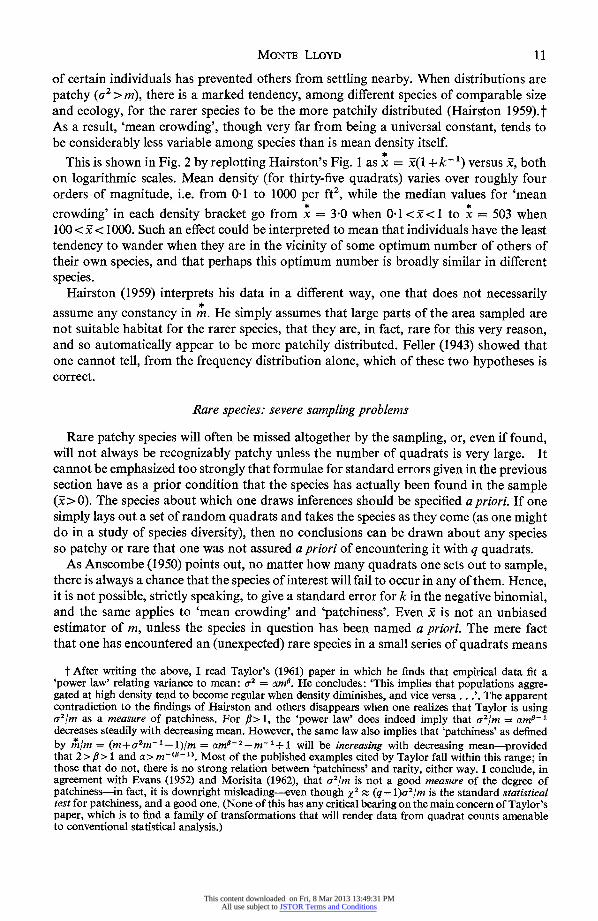
This has already been demonstrated in an important paper by Morisita (1959a), who set out to design a measure of patchiness, I&, that would not change with quadrat size. Though independently derived, from quite different considerations, the ratio of 'mean

crowding' to mean density (x/x), which I propose here as a measure of patchiness turns out to be essentially identical with Morisita's parameter I:

q Z xj(xj-l) * *

1 [ X l (36)

(The term l/q in the denominator serves as a rough correction for sampling bias.) Under

the circumstances indicated by Morisita for which I, w x/x will be independent of

quadrat size, therefore, one should find that x/= (x/x)(5/0) is also, since x/0 is merely an unbiased estimator of mean density (for an expected species) in standard units.

0 F ~~~SuitabLe range for 8 o

a.'

Quadrat size (9)

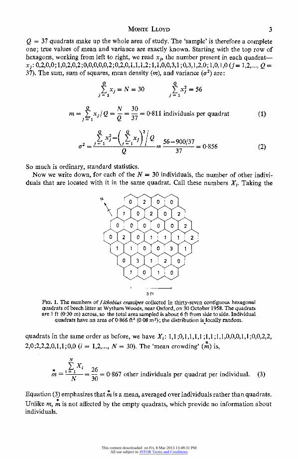
FIG. 3. The relation postulated by Morisita (1959a) between quadrat size and I,, his measure of patchiness (which is approximately equivalent to the measure xlx proposed in the present paper). Morisita is assuming local randomness, i.e. that the individuals position themselves at random with respect to one another within a clump, and that the clumps themselves are large relative to quadrat size. The measure of patchiness is independent of quadrat size so long as quadrats are small enough that negligibly few of them straddle clump boundaries. When quadrats become too large, the degree of patchiness is obscured: 1d declines towards unity ( - - ), its expectation in a random distribution. Empirically, a given convenient quadrat size (0) can be identified as probably lying within the 'suitable range' if a series of contiguous quadrats of size 0 fit a Poisson series, provided the quadrats

are large in comparison with the space occupied by the animals' bodies.

Where the distribution is locally random, yet the mean density changes slowly from place to place-an assumption consistent with the negative binomial-Morisita shows that if q is large his Ij is constant for all quadrat sizes below a certain critical maximum, coinciding roughly with the 'patch' size within which mean density remains uniform. For quadrats larger than that, Ij declines monotonically, as shown in Fig. 3. In other words, the quadrat size must be smaller than the scale on which changes in mean density take place, in order to 'reveal' all the patchiness that exists. One might wish to take an interest in the pattern of patchiness on a very much larger scale, as many plant ecologists do



16 'Mean crowding'

(Goodall 1952; Pielou 1960; Grieg-Smith 1961), but this has little relevance to an animal's experience of crowding if that scale lies far beyond its ambit.

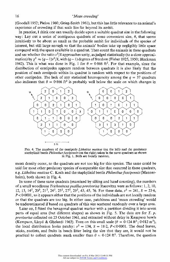
In practice, I think one can usually decide upon a suitable quadrat size in the following way: Lay out a series of contiguous quadrats of some convenient size, 0, that seems intuitively to be about as small as the probable ambit for individuals of the species of interest, but still large enough so that the animals' bodies take up negligibly little space compared with the space available in a quadrat. Then count the animals in these quadrats and see whether the ratio S2/X approaches unity, as judged statistically (to a close approxi- mation) by X2 - (q- 1)s2/5, with (q- 1) degrees of freedom (Fisher 1925, 1950; Blackman 1942). This is what was done in Fig. 1 for 0 = 0-866 ft2. For that example, since the distribution of centipedes appears random between quadrats it is also likely that the position of each centipede within its quadrat is random with respect to the positions of other celntipedes. The lack of any statistical heterogeneity among the q = 37 quadrats also indicates that 0 = 0-866 ft2 is probably well below the scale on which changes in

2 1 1 0 1 1 31 0

1 0 0 0 1 0 2

3 ft

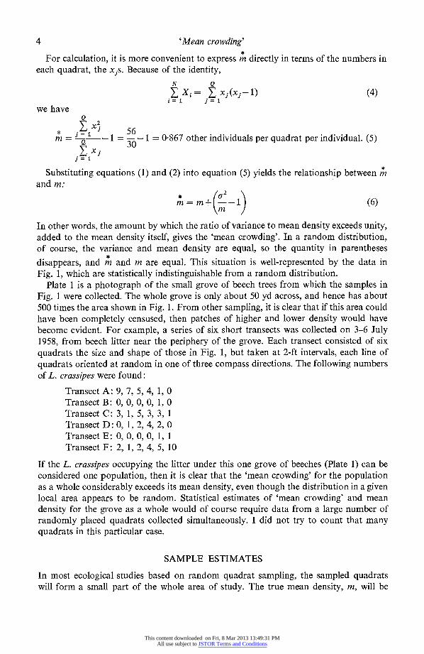
FIG. 4. The numbers of the centipede Lithobius muticus (on the left) and the predatory staphylinid beetle Philonthus fuscipennis (on the right) taken in the same quadrats as shown

in Fig. 1. Both are locally random.

mean density occur, so the quadrats are not too big for this species. The same could be said for most other predatory species of comparable size that occurred in these quadrats, e.g. Lithobius muticus C. Koch and the staphylinid beetle Philonthusfuscipennis (Manner- heim), both shown in Fig. 4.

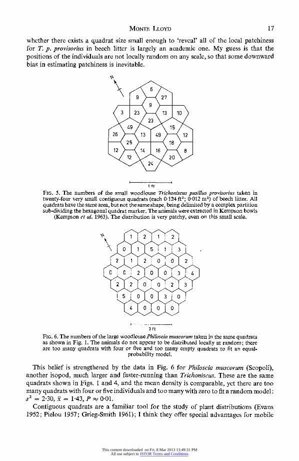
In some of these same quadrats (examined by sifting and hand counting), the numbers of a small woodlouse Trichoniscus pusillus provisorius Racovitza were as follows: 1, 2, 10, 12, 13, 142, 203, 212, 242, 252, 272, 292, 43, 45, 76. For these data, S2 = 241, x = 23-6, P<00001, so it appears either that the positions of the individuals are not locally random or that the quadrats are too big. In either case, patchiness and 'mean crowding' would be underestimated if based on quadrats of this size scattered randomly over a large area.

Later on, I fitted the hexagonal quadrat marker with a partition dividing it into seven parts of equal area (but different shapes) as shown in Fig. 5. The data are for T. p. provisorius collected on 25 October 1961, and extracted without delay in Kempson bowls (Kempson, Lloyd & Ghelardi 1963). Even on this small scale (0 = 04124 ft2; 0-012 m2),

the local distribution looks patchy: S2 = 134, - = 18-2, P<0-0001. The dead leaves, sticks, rootlets, and fruits in beech litter being the size that they are, it would not be practical to collect quadrats much smaller than 0 = 0K124 ft2. Therefore, the question



MONTE LLOYD 17

whether there exists a quadrat size small enough to 'reveal' all of the local patchiness for T. p. provisorius in beech litter is largely an academic one. My guess is that the positions of the individuals are not locally random on any scale, so that some downward bias in estimating patchiness is inevitable.

(3 23 ><13 10

25 18

12 14. 16 8 122

1 ft

FIG. 5. The numbers of the small woodlouse Trichoniscus pusillus provisorius taken in twenty-four very small contiguous quadrats (each 0-124 ft2; 0-012 m2) of beech litter. All quadrats have the same area, but not the same shape, being delimited by a complex partition sub-dividing the hexagonal quadrat marker. The animals were extracted in Kempson bowls

(Kempson et al. 1963). The distribution is very patchy, even on this small scale.

50 0 30

2

2 0 0 0

3 ft

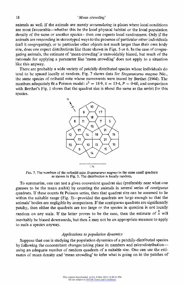
FIG. 6. The numbers of the large woodlouse Philoscia muscorum taken in the same quadrats as shown in Fig. 1. The animals do not appear to be distributed locally at random; there are too many quadrats with four or five and too many empty quadrats to fit an equal-

probability model.

This belief is strengthened by the data in Fig. 6 for Philoscia muscorum (Scopoli), another isopod, much larger and faster-running than Trichoniscus. These are the same quadrats shown in Figs. 1 and 4, and the mean density is comparable, yet there are too many quadrats with four or five individuals and too many with zero to fit a random model: s2 =2-30,= 143,P- 001.

Contiguous quadrats are a familiar tool for the study of plant distributions (Evans 1952; Pielou 1957; Grieg-Smith 1961); I think they offer special advantages for mobile



18 'Mean crowding'

animals as well. If the animals are merely accumulating in places where local conditions are most favourable-whether this be the local physical habitat or the local population density of the same or another species-then one expects local randomness. Only if the animals are responding in stereotyped ways to the presence of particular other individuals (call it congregating), or to particular other objects not much larger than their own body size, does one expect distributions like those shown in Figs. 5 or 6. In the case of congregating animals, the estimate of 'mean crowding' is unavoidably biased, but much of the rationale for applying a parameter like 'mean crowding' does not apply to a situation like this anyway.

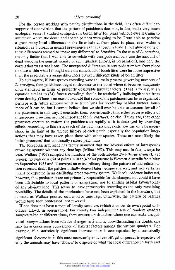
There are probably a wide variety of patchily distributed species whose individuals do tend to be spaced locally at random. Fig. 7 shows data for Steganacarus magnus Nic., the same species of oribatid mite whose movements were traced by Berthet (1964). The numbers adequately fit a Poisson model: S2 = 18-9, = 13-4, P = 0-60, and comparison with Berthet's Fig. I shows that the quadrat size is about the same as the ambit for this species.

17 21

9 > 15

1 ft

FIG. 7. The numbers of the oribatid mite Steganacarus magnus in the same small quadrats as shown in Fig. 5. The distribution is locally random.

To summarize, one can test a given convenient quadrat size (preferably near what one guesses to be the mean ambit) by counting the animals in several series of contiguous quadrats. If these counts fit Poisson series, then that quadrat size can be assumed to lie within the suitable range (Fig. 3)-provided the quadrats are large enough so that the animals' bodies are negligible by comparison. If the contiguous quadrats are significantly patchy, then either the quadrats are too large or the species in question is not locally

random on any scale. If the latter proves to be the case, then the estimate of x will

inevitably be biased downwards, but then x may not be an appropriate measure to apply to such a species anyway.

Applications to population dynamics

Suppose that one is studying the population dynamics of a patchily-distributed species. by following the concomitant changes taking place in numbers and microdistribution- using an adequate number of random quadrats of a suitable size. One can use the estimates of mean density and 'mean crowding' to infer what is going on in the patches of



MONTE LLOYD 19

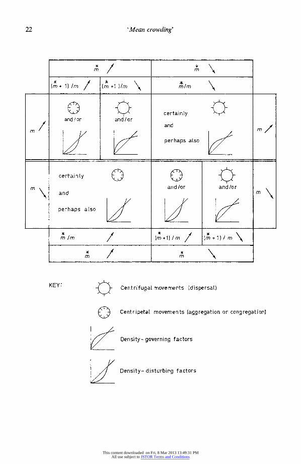
locally different density, without actually locating these patches and studying them individually (see Fig. 8). For example, suppose a general increase in numbers occurs, owing to factors that operate independently of local density. In that case, the proportional increases will be the same in patches of locally high and locally low density. Mean density will increase and so will 'mean crowding', but patchiness (the ratio between them) should remain the same-or so one might at first suppose.

Strictly speaking, however, it is not patchiness itself, but the ratio (im + )/rm that should remain constant. This is so because the 'subjective' individual would be as likely to reproduce as those around it, and this individual was left out of account in defining m, although of course it is included in m. To put it another way, we can write (m + 1)/m I+k-'+rMl = 1+(F2/rM2). Now let every quadrat with xj individuals change by a factor C to contain C Xj individuals. The new mean is Cm, the new variance is C2U2,

and one sees that (m + 1)/m 1 + (C%2/C2r2)=+ ( (c/r2) remains unchanged. Standard errors for the sample estimates, (x + 1)/9 1 + Ik' + x,- 1 appropriate to each of the four methods of estimating k in the negative binomial, are indicated in the caption for Fig. 8. One does, therefore, expect changes in patchiness associated with density- independent mortality or natality. but, since [(ml/m) + (1/rm)] remains constant, these changes will be no greater than the changes in the reciprocals of the mean densities. Moreover, if there is no long-term change in mean abundance then there will be none in patchiness either.

On the other hand, suppose mortality is density-dependent, falling more heavily on the patches of locally high density. In this case, (mA + 1) will decrease proportionately more than m. The quantity [(Mz/m)+(l1/m)] will decrease, in other words, and since (1/m) is increasing, the patchiness (mA/m) will certainly decrease. Next consider what happens with a density-dependent increase in numbers. If the rate of increase is especially depressed in patches of locally high density, then (mA + 1) will increase proportionately less than m. Again, the quantity [(m/m) + (1/rm)] will decrease, but in this case (1/rm) is also decreasing, so one cannot in general say in which direction patchiness will change. What one can say, however, is that the operation of density-dependent factors continually tends to decrease the quantity [(m/m) +(1/rm)] and that unless there is a long-term increase in numbers of considerable magnitude, this will inevitably result in a decrease in the overall patchiness. This being the case, does not the very fact that patchy distributions persist in nature (and numbers are not continually increasing) suggest that these populations are not regulated by intraspecific density-dependent processes?

This unorthodox suggestion serves to point up the most critical assumption implicit in interpreting the parameter x = x41 +k- ) in the way that I have: the assumption that all the quadrats afford the same rate of supply of resources or have the same amount of 'room' (cover) which animals can use to avoid each other. This assumption is tantamount to saying that the patchy distribution itself does not make any ecological sense-unless the animals are merely attracted to one another's presence, in which case why speak of 'crowding' at all, much less of 'crowding' as the process that regulates numerical abundance? The two ideas seem incompatible, since if numbers are being governed only by effects of intraspecies crowding, there will be strong natural selection favouring those individuals that avoid others of their kind; natural distributions should exhibit no more patchiness than is necessitated by the patchiness in habitat factors.



20 'Mean crowding'

For the person working with patchy distributions in the field, it is often difficult to suppress the conviction that the pattern of patchiness does not, in fact, make very much ecological sense. I studied centipedes in beech litter for years without ever learning to anticipate where the dense and sparse patches were going to be. I was able to perceive a great many local differences in the litter habitat from place to place, even within a situation as uniform in general appearance as that shown in Plate 1, but almost none of these differences seemed to 'make any difference' to Lithobius. In the case of L. crassipes, the only factor that I was able to correlate with centipede numbers was the amount of dead wood in the general vicinity of each quadrat (Lloyd, in preparation), and here the correlation was a weak one. The unexpected differences in centipede numbers from place to place within what I thought were the same kind of beech litter were far more impressive than the predictable average differences between different kinds of beech litter.

To summarize, if intraspecies crowding were the main process governing numbers of L. crassipes, then patchiness ought to decrease to the point where it becomes completely understandable in terms of presently observable habitat factors. (That is to say, in an equation similar to (34), 'mean crowding' should be statistically indistinguishable from mean density.) There is no reason to doubt that some of the patchiness can be so explained; perhaps with future improvements in techniques for measuring habitat factors, much more of it can be, but I cannot believe that we shall ever be able to account for all of the patchiness in this way. I conclude, then, provisionally, that either adverse effects of intraspecies crowding are not important for L. crassipes, or else, if they are, that other processes operate to restore the patchiness as rapidly as it is destroyed by crowding effects. According to this view, much of the patchiness that exists now can only be under- stood in the light of the unique history of each patch, especially the population interactions that may have taken place there with other species. These are most likely the 'other processes' that continually restore patchiness.

The foregoing argument has tacitly assumed that the adverse effects of intraspecies crowding operate without any time lags (Milne 1957). This may not, in fact, always be true. Wallace (1957) sampled -the numbers of the collembolan Sminthurus viridis (L.) at 3-week intervals on a grid of points in 10 ac (4 ha) of pasture in Western Australia from May to September 1953 and discovered an extraordinary thing: the pattern of microdistribution reversed itself, the patches initially densest later became sparsest, and vice versa, as might be expected in an oscillating predator-prey system. Wallace's evidence indicated, however, that predators were not primarily responsible for the changes, nor could it have been attributable to local patterns of emigration, nor to shifting habitat favourability of any obvious kind. This seems to leave intraspecies crowding as the only remaining possibility. The details of the mechanism have not been explained in the literature, but it must, as Wallace pointed out, involve time lags. Otherwise, the pattern of patches would have been obliterated, not reversed.

If one does not have a map of density contours (which involves its own special difficulties: Lloyd, in preparation), but merely two independent sets of random quadrat samples taken at different times, there are certain situations where one can make unequi-

vocal interpretations from relative changes in I and x, notwithstanding the doubts one may have concerning equivalence of habitat factors among the various quadrats. For example, if a statistically significant increase in x is accompanied by a statistically

significant decrease in x, this must necessarily entail centrifugal dispersal, irrespective of why the animals may have 'chosen' to disperse or what the local differences in birth and



MONTE LLOYD 21

death rates may be. The available interpretations are summarized in Fig. 8. Some interesting work along these lines has already been done by Kaczmarek (1960), who found in certain collembolan species an inverse relation through time between mean density and a parameter related to patchiness. In a later paper I will apply the method to successive stages of periodical cicadas.

'MEAN CROWDING' BETWEEN SPECIES

One can obviously extend equation (8) to apply to 'mean crowding' between species, or between life history stages of one species, where these are mixed and interact. As a crude estimate, we have X12, the 'mean crowding' on species 1 by species 2:

q

E XljX2j

X12= q

Xjj

where xIj and X2j are the numbers in the jth quadrat of species 1 and 2 respectively. Similarly, we have the 'mean crowding' on species 2 by species 1:

q

XljX2j

X2 1- -q (38)

jEX2i

It is clear from the work of Morisita that under the same conditions where the measures of intraspecies patchiness (call them x, 11 and x22/2) are practically independent of quadrat size, the measures of interspecies patchiness (*2/x1 and x*2/x2) will be also. Morisita (1959b) shows that his 'index of interspecies overlapping', Ca, is almost independent of quadrat size. This parameter can be written as follows:

q 2 XljX21 2 1j2

(21/15) + (X* 1 2/X2)

C,a* (39) q 5x152 (IJI +I32) (X11/X5)+(X22/15)

Hence, I assume that either of the two terms in the numerator on the right will be almost unaffected by quadrat size (0) and this should also be true for 'mean crowding' between species when expressed in standard units of area, x12/0 and X21/0.

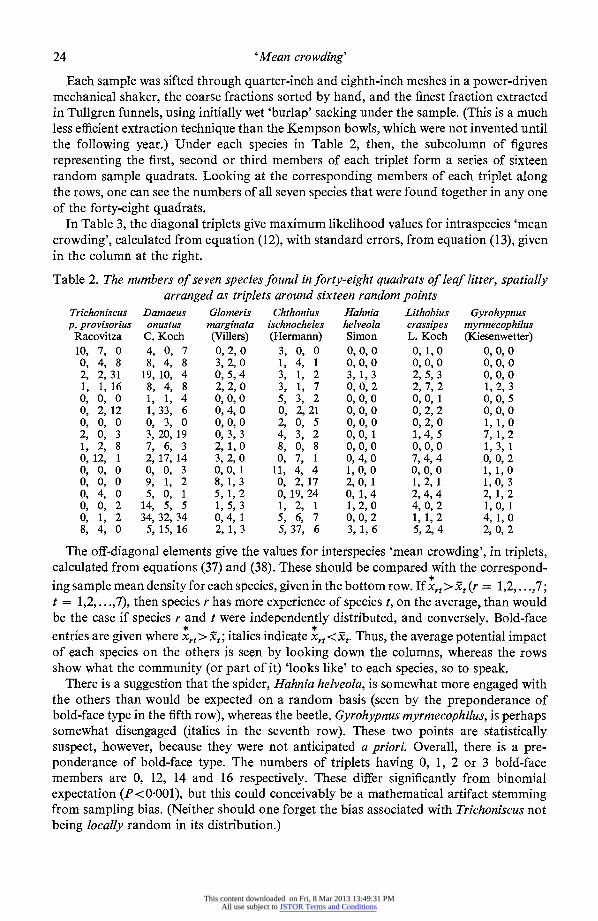
The data in Table 2 will serve as a numerical example, although the samples were collected for a different purpose and are not nearly extensive enough to do justice to this one. Numbers are recorded for seven species: a woodlouse-Trichoniscus pusillus provisorius; an oribatid mite-Damaeus onustus; an oniscomorph millipede-Glomeris marginata; a pseudoscorpion-Chthonius ischnocheles; a small agelenid spider-Hahnia helveola; a centipede-Lithobius crassipes; and a staphylinid beetle-Gyrohypnus myrmecophilus. Each triplet of figures in Table 2 shows the numbers collected in three hexagonal quadrats (0 = 0-866 ft2) placed at the vertices of a triangle 5 2 ft (1.58 m) on a side, randomly placed in the grove pictured in Plate 1, during May 1959. The leaf litter was stored in double polyethylene bags in a shed at outdoor temperatures, and the animals extracted from one triplet of samples at a time, the last extraction not being completed until late in June.



22 'Mean crowding'

m /|m \

(m+ 1)/n / (m +1)/m m/m

( ) ) X ~~~~~certainlyX and /or and/or

/ I ~~~~~~~~~andrn

perhaps also

certainly |iil m a and/or and/or

perhaps also

| m/m /m | (m+1)/rM (mr+1)/ m

l ~ ~m /|m\l

KEY: Centrifugal movements (dispersal)

O Centripetat movements (aggregation or congregation)

Density- governing factors

Density- disturbing factors



MONTE LLOYD 23

FIG. 8. The available interpretations of relative changes in 'mean crowding', m (estimated

by x) and mean density, m (estimated by x). Upward arrows show increases; downward

arrows, decreases. Symbols for the operation of density-governing and density-disturbing *

factors (Nicholson 1954) are borrowed from Ricker's (1954) reproduction curves. When m

and m change in opposite directions, the 'patchiness' (mlm) necessarily changes in the same

direction as m, and at least part of the change can be attributed unequivocally to centripetal

or centrifugal movements. When m and m change in the same direction, inferences can

most readily be made by testing the ratio (m+ 1)/rm, which should be invariant under the

operation of density-independent factors. Standard errors for estimates of this ratio are

indicated below.

For estimation of k by maximum likelihood:

* S.E. [(x+ 1)/x]= ]/ ({formula (16)}2 + {formula (17)/x2}2)

For estimation of k by moments:

S.E. [(xl + l)/I]= ({formula (20)}2 +s2/qx4)

For estimation of k by empty quadrats:

S.E. [(x2+ 1)/xl] >/ ({formula (23)}2+(k2I +x g)/qx2)

For estimation of k in the truncated negative binomial by 'Method A' of Brass (1958):

S.E [(X3 + 1)/M]= V/ ({formula (33)}2 + {formula (31)1M2}2-2 coy (w, f3)If3w,M2)

where w(k3 + 1) 1k3 (2 -3P) +P (1 - w') (k2 +4k3 +2)+P2 (k3 + 1 - WV)1

coY (w, Ik;3)- qt(l -P)2 (k3 - W/3 +P)

M= k3(1- 0)Hwi and P=qllqt.

If m, m, and m/m all change in the same direction, nothing can be concluded unless a com-

parable change can also be demonstrated in (m+ 1)/rm. On the other hand, if it can be * ~~~~~~~~~~~~*

shown that m/m has changed in a direction opposite to that of m and m, then it necessarily

follows that (mr+ 1)/m has also, but testing (mr+ 1)/m directly will usually be a more sensitive

means of detecting departures from density-independence.



24 'Mean crowding'

Each sample was sifted through quarter-inch and eighth-inch meshes in a power-driven mechanical shaker, the coarse fractions sorted by hand, and the finest fraction extracted in Tullgren funnels, using initially wet 'burlap' sacking under the sample. (This is a much less efficient extraction technique than the Kempson bowls, which were not invented until the following year.) Under each species in Table 2, then, the subcolumn of figures representing the first, second or third members of each triplet form a series of sixteen random sample quadrats. Looking at the corresponding members of each triplet along the rows, one can see the numbers of all seven species that were found together in any one of the forty-eight quadrats.

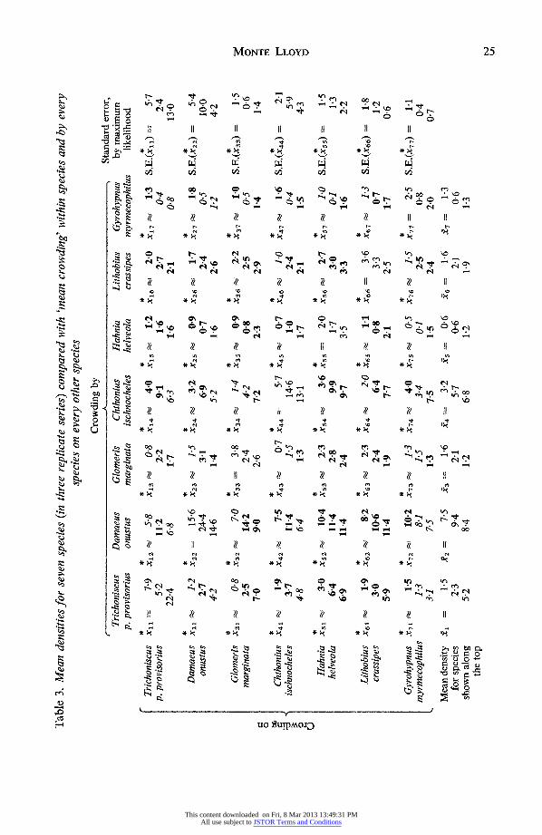
In Table 3, the diagonal triplets give maximum likelihood values for intraspecies 'mean crowding', calculated from equation (12), with standard errors, from equation (13), given in the column at the right.

Table 2. The numbers of seven species found in forty-eight quadrats of leqf litter, spatially arranged as triplets around sixteen random points

Trichoniscus Damaeus Glomeris Chthonius Hahnia Lithobius Gyrohypnus p. provisorius onustus marginata ischnocheles helveola crassipes myrmecophilus

Racovitza C. Koch (Villers) (Hermann) Simon L. Koch (Kiesenwetter) 10, 7, 0 4, 0, 7 0,2,0 3, 0, 0 0,0,0 0, 1,0 0,0,0 0, 4, 8 8, 4, 8 3,2,0 1, 4, 1 0,0,0 0,0,0 0,0,0 2, 2,31 19, 10, 4 0,5,4 3, 1, 2 3, 1,3 2,5,3 0,0,0 1, 1,16 8, 4, 8 2,2,0 3, 1, 7 0,0,2 2,7,2 1,2,3 0, 0, 0 1, 1, 4 0,0,0 5, 3, 2 0,0,0 0,0, 1 0,0,5 0, 2, 12 1,33, 6 0,4,0 0, 2,21 0,0,0 0,2,2 0,0,0 0, 0, 0 0, 3, 0 0,0,0 2, 0, 5 0,0,0 0,2,0 1, 1,0 2, 0, 3 3,20, 19 0,3,3 4, 3, 2 0,0,1 1,4,5 7,1,2 1, 2, 8 7, 6, 3 2,1,0 8, 0, 8 0,0,0 0,0,0 1,3, 1 0, 12, 1 2, 17, 14 3,2,0 0, 7, 1 0,4,0 7,4,4 0,0,2 0, 0, 0 0, 0, 3 0,0,1 11, 4, 4 1,0,0 0,0,0 1, 1,0 0, 0, 0 9, 1, 2 8,1,3 0, 2,17 2,0,1 1,2,1 1,0,3 0, 4, 0 5, 0, 1 5,1,2 0,19,24 0,1,4 2,4,4 2,1,2 0, 0, 2 14, 5, 5 1,5,3 1, 2, 1 1,2,0 4,0,2 1,0, 1 0, 1, 2 34,32,34 0,4,1 5, 6, 7 0,0,2 1,1,2 4,1,0 8, 4, 0 5, 15, 16 2,1,3 5,37, 6 3,1,6 5,2,4 2,0,2

The off-diagonal elements give the values for interspecies 'mean crowding', in triplets, calculated from equations (37) and (38). These should be compared with the corresponding sample mean density for each species, given in the bottom row. If Xrt > Xt (r =-12 . *7; t= 1,2, .. .,7), then species r has more experience of species t, on the average, than would be the case if species r and t were independently distributed, and conversely. Bold-face entries are given where Xrt > Xt; italics indicate Xrt < Xt. Thus, the average potential impact of each species on the others is seen by looking down the columns, whereas the rows show what the community (or part of it) 'looks like' to each species, so to speak.

There is a suggestion that the spider, Hahnia helveola, is somewhat more engaged with the others than would be expected on a random basis (seen by the preponderance of bold-face type in the fifth row), whereas the beetle, Gyrohypnus myrmecophilus, is perhaps somewhat disengaged (italics in the seventh row). These two points are statistically suspect, however, because they were not anticipated a priori. Overall, there is a preponderance of bold-face type. The numbers of triplets having 0, 1, 2 or 3 bold-face members are 0, 12, 14 and 16 respectively. These differ significantly from binomial expectation (P<0f001), but this could conceivably be a mathematical artifact stemming from sampling bias. (Neither should one forget the bias associated with Trichoniscus not being locally random in its distribution.)



Table 3. Mean densities for seven species (in three replicate series) compared with 'meani crowding' within species and by every species on every other species

Crowding by Standard error,

Trichoniscus Damaeus Glomeris Chthonius Hahnia Lithobius Gyrohypnus by maximum p. provisorius onustus marginata ischnocheles helveola crassipes myrmecophilus likelihood

C * * * * * * * * Trichoniscus Xi , 7.9 X12 5^8 X13 08 x14 40 xi 15 1-2 x16 2-0 x17 1-3 S.E.(xll) = 57

p. provisorius 5-2 11-2 2-2 941 1-6 2-7 0-4 2 4 22 4 6-8 1-7 6-3 1-6 2-1 0-8 13-0

* * * * * * * * Damaeus X21 P12 X22 = 15-6 X23 P15 x24 3-2 x25 09 x26 1-7 x27 1-8 S.E.(x22) = 5-4

onustus 2-7 24-4 3-1 6-9 0 7 2-4 0 5 10 0 4-2 14-6 1 4 5 2 1-6 2-6 1-2 4-2

* * * * * * * * Glomeris X31 '08 X32 7 0 X33= 3-8 X34 1-4 X35 0 9 x36 2-2 X37 10 S.E.(x33) = 1-5

marginata 2 5 14-2 2-4 4-2 0-8 2-5 0 5 0-6 70 9*0 2-6 7*2 2-3 29 1F4 1 4 z

0

ChthoniUS X41 1.9 X42 7-5 X43 0-7 X44 = 5-7 x45, 0-7 X46 PCO X47 1F6 S.EA(X44) = 2.1 t . ischnocheles 3-7 11^4 15 146 1 0 2-4 0-4 5.9 0 1 48 64 1-3 13-1 17 21 15 43

Hahnia X5s 3 0 X52 104 X53 23 X54 36 x55 = 20 x56 27 x57 J10 S.E.(x55) = 15 helveola 6-4 11-4 2-8 9 9 1P7 3 0 01 1P3

6-9 11-4 2-4 9 7 3-5 3-3 1-6 2-2 * * * * * * * *

Lithobius X61 1-9 x62 8-2 x63 2-3 x64 2-0 x65 11 x66 = 3-6 x67 1-3 S.E.(x66) 1-8 crassipes 3-0 10-6 2-4 6-4 0-8 3-3 07 1 2

5 9 11-4 1.9 7-7 2-1 2-5 1F7 0-6

Gyrohypnus x71 1-5 x72 10-2 X73 1-3 X74 40 X75 0-5 X76 P15 X77 = 2-5 S.EA(x77)= 11 myrmecophilus 1-3 8-1 15 3-4 01 2-5 0-8 0 4

3-1 7 5 1F3 7-5 1F5 2A4 2-0 0 7 Mean density = 1-5 x2 7-5 33 1-6 X = 3-2 5 = 0-6 x6 = 1*6 7 = 13

for species 2-3 9 4 2-1 5-7 0-6 2-1 0-6 shown along 5-2 8-4 1-2 6-8 1P2 19 1-3

the top



26 'Mean crowding'

Unhappily, I have not been able to work out a large-sample standard error for interspecies 'mean crowding'. Some idea of the inconsistency to be expected in successive estimates can be got by comparing the figures within triplets. However, these are only replicates within spatial blocks, not wholly independent replicates. Successive estimates based on wholly independent sets of sixteen random quadrats would of course tend to be even more inconsistent than the triplets in Table 3. Clearly one needs many more than sixteen quadrats even to attempt this kind of analysis, and this in turn requires special techniques for extracting large numbers of samples simultaneously (see Kempson et al. 1963).

Perhaps there is only one valid point that can be made from Tables 2 and 3, but it is well to emphasize it: the fact of patchy distributions in all the species means that the experience of any one species which individuals of another species can have is exceedingly variable from individual to individual-much more so than would be expected if distributions were random.

'SUBJECTIVE' SPECIES DIVERSITY

The well-known information theory measure

H(s) = T-log2(T!/xl X2! X..x!) - Pr l1g2 Pr (40)

(the rth species has xr individuals, there are T total individuals in all s species, and Pr xrIT) is an attractive way to measure species diversity, because H(s) relates to the uncertainty an individual animal has concerning which species it is going to encounter next in its wanderings through the habitat. This is important to know, because it may have a direct relationship with the stability of populations that make up the community (cf. MacArthur 1955). Thus, we have the seeming paradox of unpredictability of encounter on the individual level (= high species diversity) leading to greater predictability on the population level (= stability), being associated with a higher state of organization and 'maturity' in the whole ecosystem (Margalef 1963), and this in turn providing more reliable cues to the individual (= greater predictability) about the opportunities available to it for making a living.

If H(s) is to be interpreted as a measure of subjective uncertainty, then it seems important that it should be calculated in a way that does not assume random spatial distribution of the individuals. Lloyd & Ghelardi (1964) suggested the 'local' point of view, i.e. one should calculate the average local diversity, H(s), rather than the diversity of average local frequencies, or of overall frequencies. As an extension of that idea, one can see that average subjective uncertainty might be rather different for different species in the community, owing to the complex pattern of patchy distributions. For a particular species, call it rho, having x,,i individuals in the jth quadrat, one can write the following measure of 'subjective' species diversity, as it exists in a finite universe of Q quadrats:

Q

EXO (1J-1) 92 T !/xl!x2j!...(xp;-1) ! . ... X (j4]

Hp Q (41)

l;Xpj j = 1

where the total individuals of all species in the jth quadrat is

Ti = E Xrj (42) r = 1



MONTE LLOYD 27

(Calculation of H. is greatly facilitated by tables giving logarithms of factorials, e.g. Hald 1952.) Formula (41) is exactly like the definition of 'mean crowding' given in formulae (4) and (5), except that instead of (x,j - 1), the number of other individuals of the same species, I have substituted H(s), the diversity of all other individuals in the quadrat, of whatever species.

So far as I know, data are not available for any ecosystem that would permit one to say *

just how much Hp actually does vary from species to species. It would require either a complete census of all Q quadrats or else an adequate sampling theory that would enable

one to disentangle the true variations in H. from sampling errors-a theory I am unable to provide. *

Assuming that interspecies variation in H. is large, there may be an opportunity here to test the hypothesis that subjective uncertainty of encounter is related to population stability. If it really is, then one should be able to demonstrate an inverse relation,

*

among the species, between H. and temporal variability in mean density, 5j.-even within the same ecosystem. With enough species involved, one might be able to perceive the relationship, if there is one, despite the sampling errors. One would need, of course, to avoid being misled by changes in abundance associated merely with shifts in age distribution (Lloyd 1964), but that problem could be circumvented by taking one's samples in the same season, a year apart.

As a measure of the overall average 'subjective' species diversity existing at any one *

time, one can simply average H. over all species:

* 1 s*

H(s)=- E Hp (43) Sp= 1

(weighting each species equally). In general, H(s) will be much less than H(s) for the

whole community, but H(s) has much more relation to the subjective uncertainty of encounter faced by a typical individual of a randomly chosen species, especially if quadrat size and ambit are approximately the same. Indeed, H(s) can be regarded as a special

*

case of H(s), the case where ambit sizes are the largest possible, i.e. where all individuals of all species wander at random over the entire ecosystem.

ACKNOWLEDGMENTS

My ideas on patchy distributions were developed at the Bureau of Animal Population in Oxford, first as a United States National Science Foundation post-doctoral fellow and later under a research grant from the British Nature Conservancy. The data on cicada burrows and in Figs. 5 and 7 were collected as parts of two later research projects, both funded by the National Science Foundation through the University of California at Los Angeles, and held jointly with other investigators: one (GB550) with Henry Dybas of the Chicago Natural History Museum, the other (GB50) with Ray Ghelardi, now with the Fisheries Research Board of Canada, Nanaimo, B.C.

I am most grateful to the Director of the Bureau of Animal Population, Mr Charles Elton, F.R.S., for stimulating discussions and for having provided me with unlimited time to think. Several mathematicians gave me help, especially P. H. Leslie of the B.A.P.; I



28 'Mean crowding'

also had useful discussions and correspondence with J. G. Skellam, David Kendall, Richard Lewontin, W. Brass, and E. C. Pielou. I benefited from many long discussions with visitors and students at the B.A.P., especially with Peter Larkin and William Murdoch, and more recently with James Enright and Alan Chapman at U.C.L.A. The chief technician at the B.A.P., Mr Denys Kempson, designed and built the sampling equipment and helped in many other ways as well.

A shortened version of this paper was presented as a talk to the Ecological Society of America on 28 December 1965, at a symposium on 'Diversity and abundance in natural communities'.

SUMMARY

Patchy distributions matter, from the point of view of the animals involved, because the individuals tend to find more others of their own kind right around them than would be the case in a random distribution. The animals are more 'crowded', in this sense, than their mean density would lead one to believe. For data from randomly placed quadrats,

the proposed parameter 'mean crowding' (m) attempts to measure this effect by defining the mean number per individual of other individuals in the same quadrat. 'Mean crowding' is algebraically identical with mean density, augmented by the amount the ratio of

variance to mean exceeds unity, i.e. mz = m + (r2/m) -1. It can be viewed as equal to that increased mean density which a patchily distributed population could have, and be no more 'crowded' on the average than it is now, if it had a random distribution. The contention that populations with differing mean densities but the same 'mean crowding' would suffer the same density-dependent effects on mortality, natality, and dispersal implies the untested assumption that the effect of crowding on each individual varies linearly with the number of others around it, which are responsible for the crowding.

Also implied is that each local situation (quadrat) is equally good habitat for the animals, has an equal rate of supply of expendable resources, and provides an equal amount of 'room', or cover, which the animals can use to avoid each other. If this assumption is perfectly fulfilled, however, then the patchy distribution itself becomes an ecological enigma: if the effects of crowding are more severe in the locally densest patches, then the local density should decrease more rapidly and increase more slowly there than elsewhere. The overall patchiness should decrease, in fact, until the distribution eventually comes to resemble a random one.

Undoubtedly, a great deal of the patchiness that one finds in continuous habitats can be explained in terms of local differences in habitat suitability. On the other hand, there is often a large component that appears to be utterly capricious. Since all of the capricious component should long since have been eroded away by density-dependent effects of crowding-if these are important-I must conclude that they are not important in such species, or, if they are, that other population processes (e.g. interactions with other species) regenerate patchiness as rapidly as it is destroyed. This fits in well with a general conviction that patchiness has a great deal more to do with undercrowding than with overcrowding, since 'mean crowding' often appears to be as great in rare species as it is in common ones (of comparable size).

A suitable measure of patchiness is the ratio of 'mean crowding' to mean density. Where the distribution can be adequately approximated by the negative binomial, with

parameters m and k, we have Mrnm = I k -. The sample estimate for 'mean crowding'



MONTE LLOYD 29

is x = x(1 + - 1). Standard errors are given for the cases where k is estimated by maximum likelihood, by moments, by the number of empty quadrats, and also for the truncated negative binomial. The idea is briefly extended to apply to 'mean crowding' between species and to 'subjective' species diversity, without attempting in these cases to develop standard errors.

Most importantly, I have tried to specify the types of habitats and distributions to which the parameter 'mean crowding' is not intended to apply.

REFERENCES

Andrewartha, H. G. (1957). The use of conceptual models in population ecology. Cold Spring Harb. Symp. quant. Biol. 22, 219-36.

Anscombe, F. J. (1950). Sampling theory of the negative binomial and logarithmic series distributions. Biometrika, 37, 358-82.

Berthet, P. L. (1964). Field study of the mobility of Oribatei (Acari), using radioactive tagging. J. Anim. Ecol. 33, 443-9.

Birch, L. C. (1957). The role of weather in determining the distribution and abundance of animals. Cold Spring Harb. Symp. quant. Biol. 22, 203-18.

Blackman, G. E. (1942). Statistical and ecological studies in the distribution of species in plant communities. I. Dispersion as a factor in the study of changes in plant populations. Ann. Bot. 6, 351-70.

Blair, W. F. (1940). Home ranges and populations of the meadow vole in southern Michigan. J. Wildl. Mgmt, 4, 149-61.

Bliss, C. I. & Fisher, R. A. (1953). Fitting the negative binomial distribution to biological data and nbote on the efficient fitting of the negative binomial. Biometrics, 9, 176-200.

Brant, D. H. (1962). Measures of the movements and population densities of small rodents. Univ. Calif. Publs Zool. 62, 105-84.

Brass, W. (1958). Simplified methods of fitting the truncated negative binomial distribution. Biometrika, 45, 59-68.

Calhoun, J. B. & Casby, J. U. (1958). Calculation of home range and density of small mammals. Publ. Hlth Monogr. 55, 1-24.

Cassie, R. M. (1962). Frequency distribution models in the ecology of plankton and other organisms. J. Anim. Ecol. 31, 65-92.

Dice, L. R. & Clark, P. J. (1953). The statistical concept of home range as applied to the recapture radius of the deermouse (Peromyscus). Contr. Lab. vertebr. Biol. Univ. Mich. 62, 1-15.

Elton, C. (1949). Population interspersion: an essay on animal community patterns. J. Ecol. 37, 1-23. Evans, F. C. (1952). The influence of size of quadrat on the distributional patterns of plant populations.

Contr. Lab. vertebr. Biol. Univ. Mich. 54, 1-15. Feller, W. (1943). On a general class of 'contagious' distributions. Ann. math. Statist. 14, 389-400. Fisher, R. A. (1925). Statistical Methods for Research Workers. London. Fisher, R. A. (1950). The significance of deviations from expectation in a poisson series. Biometrics,

6, 17-24. Godfrey, G. K. (1954). Tracing field voles (Microtus agrestis) with a Geiger-Muller counter. Ecology,

35, 5-10. Goodall, D. W. (1952). Quantitative aspects of plant distribution. Biol. Rev. 27, 194-245. Greig-Smith, P. (1961). Data on pattern within plant communities. I. The analysis of pattern. II. Ammo-

phila arenaria (L.) Link. J. Ecol. 49, 695-708. Greig-Smith, P. (1964). Quantitative Plant Ecology, 2nd edn. London. Hairston, N. G. (1959). Species abundance and community organization. Ecology, 40, 404-16. Hald, A. (1952). Statistical Tables and Formulas. New York. Hayne, D. W. (1949). Calculation of the size of home range. J. Mammal. 30, 1-18. Hayne, D. W. (1950). Apparent home range of Microtus in relation to distance between traps. J.

Mammal. 31, 26-39. Johnson, C. G., Taylor, L. R. & Southwood, T. R. E. (1962). High altitude migration of Oscinellafrit L.

(Diptera: Chloropidae). J. Anim. Ecol. 31, 373-83. Kaczmarek, W. (1960). Research on the space pattern of the population of several chosen species of

Collembola. Ekol. pol., Ser. A, 8, 1-64. Kempson, D., Lloyd, M. & Ghelardi, R. (1963). A new extractor for woodland litter. Pedobiologia, 3,

1-21. Lloyd, M. (1964). Weighting individuals by reproductive value in calculating species diversity. Am.

Nat. 98, 190-2.

C J.A.E.



30 'Mean crowding'

Lloyd, M. & Ghelardi, R. J. (1964). A table for calculating the 'equitability' component of species diversity. J. Anim. Ecol. 33, 217-25.

MacArthur, R. (1955). Fluctuations of animal populations, and a measure of community stability. Ecology, 36, 533-6.

Margalef, R. (1963). On certain unifying principles in ecology. Am. Nat. 97, 357-74. Milne, A. (1957). The natural control of insect populations. Can. Ent. 89, 193-213. Morisita, M. (1959a). Measuring the dispersion of individuals and analysis of the distributional patterns.

Mem. Fac. Sci. Kyushu Univ., Ser. E, 2, 215-35. Morisita, M. (1959b). Measuring of interspecific association and similarity between communities. Mem.

Fac. Sci. Kyushu Univ., Ser. E, 3, 65-80. Morisita, M. (1962). I-index, a measure of dispersion of individuals. Res. Popul. Ecol. 4, 1-7. Nicholson, A. J. (1954). An outline of the dynamics of animal populations. Aust. J. Zool. 2, 9-65. Nicholson, A. J. (1957). The self-adjustment of populations to change. Cold Spring Harb. Symp. quant.

Biol. 22, 153-73. Nicholson, A. J. (1958). Dynamics of insect populations. A. Rev. Ent. 3, 107-36. Paviour-Smith, K. (1960). The fruiting-bodies of macrofungi as habitats for beetles of the family Ciidae

(Coleoptera). Oikos, 11, 43-71. Pielou, E. C. (1957). The effect of quadrat size on the estimation of the parameter of Neyman's and

Thomas's distributions. J. Ecol. 45, 31-47. Pielou, E. C. (1960). A single mechanism to account for regular, random and aggregated populations.

J. Ecol. 48, 575-84. Ricker, W. E. (1954). Stock and recruitment. J. Fish. Res. Bd Can. 11, 559-623. Sampford, M. R. (1955). The truncated negative binomial distribution. Biometrika, 42, 58-69. Skeliam, J. G. (1952). Studies in statistical ecology. I. Spatial pattern. Biometrika, 39, 346-62. Stickel, L. F. (1946). Experimental analysis of methods for measuring small mammal populations. J.

Wildl. Mgmt, 10, 150-9. Taylor, L. R. (1961). Aggregation, variance and the mean. Nature, Lond. 189, 732-5. Thompson, H. R. (1956). Distribution of distance to the nth neighbor in a population of randomly

distributed individuals. Ecology, 37, 391-4. Wallace, M. M. H. (1957). Field evidence of density-governing reaction in Sminthurus viridis (L.).

Nature, Lond. 180, 388-90. Watt, A. S. (1947). Pattern and process in the plant community. J. Ecol. 35, 1-22. Whittaker, R. H. (1965). Dominance and diversity in land plant communities. Science, N. Y. 147,

250-60.

(Received 20 June 1966)



Date post:	24-Jul-2019
Category:	Documents
Upload:	vanduong
View:	213 times
Download:	0 times

'MEAN CROWDING' - britishecologicalsociety.org · Mean density, therefore, is misleading as a...

Documents