Mean Reversion across National Stock Markets and Parametric Contrarian Investment Strategies RONALD BALVERS, YANGRU WU, and ERIK GILLILAND* ABSTRACT For U.S. stock prices, evidence of mean reversion over long horizons is mixed, possibly due to lack of a reliable long time series. Using additional cross-sectional power gained from national stock index data of 18 countries during the period 1969 to 1996, we find strong evidence of mean reversion in relative stock index prices. Our findings imply a significantly positive speed of reversion with a half- life of three to three and one-half years. This result is robust to alternative spec- ifications and data. Parametric contrarian investment strategies that fully exploit mean reversion across national indexes outperform buy-and-hold and standard con- trarian strategies. Mean reversion refers to a tendency of asset prices to return to a trend path. The existence of mean reversion in stock prices is subject to much contro- versy. Fama and French ~1988a! and Poterba and Summers ~1988! are the first to provide direct empirical evidence that mean reversion occurs in U.S. stock prices over long horizons. 1 Others are critical of these results: Lo and MacKinlay ~1988! find evidence against mean reversion in U.S. stock prices using weekly data; Kim, Nelson, and Startz ~1991! argue that the mean reversion results are only detectable in prewar data; and Richardson and Stock ~1989! and Richardson ~1993! report that correcting for small-sample bias problems may reverse the Fama and French ~1988a! and Poterba and Summers ~1988! results. Campbell, Lo, and MacKinlay ~1997! summarize the debate concisely: *West Virginia University, Rutgers University, and West Virginia University, respectively. We thank Jonathan Lewellen, Bill McDonald, Dilip Patro, John Wald, and conference partici- pants of the Eastern Finance Association, Western Finance Association, and the Ninth Annual Conference on Financial Economics and Accounting at the Stern School of Business of New York University for helpful conversations and comments. We are especially grateful to René Stulz ~the editor! and two anonymous referees whose comments and suggestions led to a substantial improvement in the quality of the paper. The usual disclaimer applies. We would also like to thank Morgan Stanley Capital International for providing part of the data used in this project. Balvers acknowledges the Faculty Research Associates program of the Bureau of Business and Economic Research at West Virginia University for research support. 1 As argued by Fama and French ~1988a! and confirmed by general equilibrium models of Balvers, Cosimano, and McDonald ~1990! and Cecchetti, Lam, and Mark ~1990!, mean reversion can be consistent with equilibrium in an efficiently functioning financial market. THE JOURNAL OF FINANCE • VOL. LV, NO. 2 • APRIL 2000 745
Transcript
Mean Reversion across NationalStock Markets and Parametric
Contrarian Investment Strategies
RONALD BALVERS, YANGRU WU, and ERIK GILLILAND*
ABSTRACT
For U.S. stock prices, evidence of mean reversion over long horizons is mixed,possibly due to lack of a reliable long time series. Using additional cross-sectionalpower gained from national stock index data of 18 countries during the period1969 to 1996, we find strong evidence of mean reversion in relative stock indexprices. Our findings imply a significantly positive speed of reversion with a half-life of three to three and one-half years. This result is robust to alternative spec-ifications and data. Parametric contrarian investment strategies that fully exploitmean reversion across national indexes outperform buy-and-hold and standard con-trarian strategies.
Mean reversion refers to a tendency of asset prices to return to a trend path.The existence of mean reversion in stock prices is subject to much contro-versy. Fama and French ~1988a! and Poterba and Summers ~1988! are thefirst to provide direct empirical evidence that mean reversion occurs in U.S.stock prices over long horizons.1 Others are critical of these results: Lo andMacKinlay ~1988! find evidence against mean reversion in U.S. stock pricesusing weekly data; Kim, Nelson, and Startz ~1991! argue that the meanreversion results are only detectable in prewar data; and Richardson andStock ~1989! and Richardson ~1993! report that correcting for small-samplebias problems may reverse the Fama and French ~1988a! and Poterba andSummers ~1988! results. Campbell, Lo, and MacKinlay ~1997! summarizethe debate concisely:
*West Virginia University, Rutgers University, and West Virginia University, respectively.We thank Jonathan Lewellen, Bill McDonald, Dilip Patro, John Wald, and conference partici-pants of the Eastern Finance Association, Western Finance Association, and the Ninth AnnualConference on Financial Economics and Accounting at the Stern School of Business of New YorkUniversity for helpful conversations and comments. We are especially grateful to René Stulz~the editor! and two anonymous referees whose comments and suggestions led to a substantialimprovement in the quality of the paper. The usual disclaimer applies. We would also like tothank Morgan Stanley Capital International for providing part of the data used in this project.Balvers acknowledges the Faculty Research Associates program of the Bureau of Business andEconomic Research at West Virginia University for research support.
1 As argued by Fama and French ~1988a! and confirmed by general equilibrium models ofBalvers, Cosimano, and McDonald ~1990! and Cecchetti, Lam, and Mark ~1990!, mean reversioncan be consistent with equilibrium in an efficiently functioning financial market.
THE JOURNAL OF FINANCE • VOL. LV, NO. 2 • APRIL 2000
745
Overall, there is little evidence for mean reversion in long-horizon re-turns, though this may be more of a symptom of small sample sizesrather than conclusive evidence against mean reversion—we simply can-not tell. ~p. 80!
Thus, a serious obstacle in detecting mean reversion is the absence of reli-able long time series, especially because mean reversion, if it exists, is thoughtto be slow and can only be picked up over long horizons. Standard econo-metric procedures generally lack the power to reject the null hypothesis of arandom walk in stock prices against the alternative of mean reversion. Thedetection of mean reversion is further complicated by the need to identify atrend path or fundamental value path for the asset under investigation. Famaand French ~1988a!, among others, avoid specifying a trend path by first-differencing the price series. The cost of such a transformation, however, isa loss of information that could otherwise aid in identifying a mean-reverting price component.
In this paper, we employ a panel of stock price indexes from Morgan Stan-ley Capital International ~MSCI! for 18 countries with well-developed capi-tal markets ~16 OECD countries plus Hong Kong and Singapore! for theperiod 1969 to 1996 to test for mean reversion. Under the assumption thatthe difference between the trend path of one country’s stock price index andthat of a reference index is stationary, and that the speeds of reversion indifferent countries are similar, mean reversion may be detected from stockprice indexes relative to a reference index. By considering stock price in-dexes relative to a reference index, the difficult task of specifying a funda-mental or trend path can be avoided. Additionally, the panel format allowsus to utilize the information on cross-sectional variation in equity indexes toincrease the power of the test so that mean reversion can be more easilydetected, if present.
Mean reversion has been examined most extensively for the U.S. stockmarket, though some researchers have investigated mean reversion in thecontext of international stock markets as well.2 Kasa ~1992! finds that na-tional stock indexes of Canada, Germany, Japan, the United Kingdom, andthe United States are cointegrated and share one common stochastic trend.The implication of this result is that the value of a properly weighted port-folio of shares in the markets of at least two countries is stationary and thuswill display mean reversion. Richards ~1995! criticizes Kasa’s results on the
2 Mean reversion is equivalent to stationarity ~in mean!—shocks to prices are temporary sothat returns are negatively autocorrelated at certain horizons. Mean reversion thus impliesthat returns are predictable based on lagged prices. Conversely, predictability of returns basedon lagged prices need not imply mean reversion. For example, predictable explosive processesare not mean reverting. The more general predictability of international stock prices based onattributes other than price history has received growing attention. For instance, Ferson andHarvey ~1993, 1998! use a conditional beta pricing model to explain the predictability of inter-national equity returns. Cutler, Poterba, and Summers ~1991! employ the dividend-price ratioto predict international equity returns.
746 The Journal of Finance
grounds that his use of asymptotic critical values in the cointegration testsis not appropriate. When finite-sample critical values are employed, how-ever, Richards finds no significant evidence of cointegration among a groupof 16 OECD countries, containing the five countries in Kasa’s sample. In-terestingly, he detects a stationary component in relative prices ~implyingpartial mean reversion! and reports that country-specific returns relative toa world index are predictable.
Based on a panel approach, we find significant evidence of full mean re-version in national equity indexes. In particular, we conclude that a coun-try’s stock price index relative to the world index, or to a particular referencecountry’s index, is a stationary process. The strong implication is that anaccumulated returns deficit of, say, 10 percent of a particular country’s stockmarket compared to the world should be fully reversed over time. Given anestimated half-life of three to three and one-half years in our data, thiscountry’s stock market should experience an expected total returns surplus,relative to the world index, of five percent over the next three to three andone-half years. Our results are robust to several alternative specifications andto another data set from the International Monetary Fund’s International Fi-nancial Statistics ~IFS! for 11 countries for the period 1949 to 1997.
Accordingly, we may trade on the finding of mean reversion and wouldexpect to obtain results similar to those of Richards ~1995, 1997! who imple-ments the “contrarian” strategy developed by DeBondt and Thaler ~1985! toexploit ~partial! mean reversion across national stock markets.3 We devise aparametric contrarian strategy that efficiently exploits the information on meanreversion across countries directly from the parameter estimates of our econo-metric model. Comparing the average return from our parametric contrarianstrategy to that from the standard contrarian strategy, a buy-and-hold strat-egy, and a random-walk-based strategy, provides further support for the meanreversion findings and gives an estimate of the economic significance.
The remainder of the paper is organized as follows. Section I specifies theeconometric model of equity index prices and introduces the empirical meth-odology. Section II describes the data and carries out some preliminary di-agnostics of the data. Section III reports the main test results for meanreversion and Section IV investigates the robustness of the mean reversionresults. Section V studies some implications of mean reversion by introduc-ing a parametric contrarian strategy and comparing its performance againstvarious other trading rules. Section VI puts our mean reversion results inthe perspective of the literature and discusses possible explanations andSection VII presents our concluding remarks.
3 We use the term “contrarian strategy” in its general sense, as signifying buying ~selling!assets that have performed poorly ~well! in the past. The standard DeBondt and Thaler ~1985!zero-net-investment strategy ~short-selling assets that have performed well and using the pro-ceeds to buy assets that have performed poorly! is in our usage of the term just a particularexample of a contrarian strategy. The term “momentum strategy” correspondingly has the op-posite meaning.
Mean Reversion 747
I. The Econometric Model and Empirical Methodology
A typical formulation of a stochastic process for the price of an asset dis-playing mean reversion is as follows:
Pt11i 2 Pt
i 5 ai 1 li~Pt11*i 2 Pt
i! 1 et11i . ~1!
where Pti represents the log of the stock index price for country i that in-
cludes dividends at the end of year t so that ~Pt11i 2 Pt
i! equals the contin-uously compounded return an investor realizes in period t 1 1; Pt
*i indicatesthe log of the fundamental or trend value of the stock price index in countryi, which is unobserved; ai is a positive constant; and et11
i is a stationaryshock term with an unconditional mean of zero. The parameter li measuresthe speed of reversion. If 0 , li , 1, deviations of the log price from itsfundamental or trend value are reversed over time. The conventional case isli 5 0, in which the log price follows an integrated process so that there isno “correction” in subsequent periods. When li 5 1, a full adjustment occursin the subsequent period.
Empirically, to confirm mean reversion, a significant finding of li . 0 isneeded. However, in obtaining such a result, two problems arise in practice.First, it is difficult to specify the fundamental process, Pt
*i.4 Second, meanreversion, if it exists, is likely to occur slowly, and can therefore be detectedonly in long time series; yet reliable long-term data for stock returns are ingeneral hard to come by. We manage to circumvent these problems in thispaper by using the additional information in cross-country comparisons. Tothis end, we assume that the speeds of mean reversion, li, across countriesare equal and let this common value be l. Thus, the process of mean rever-sion in stock index prices need not be synchronized across countries but thespeeds at which asset prices return to their fundamental values are deemedto be similar.
We further propose that cross-country differences in fundamental stockindex values are stationary. More specifically, the fundamental values fortwo countries are assumed to be related as follows:
Pt*i 5 Pt
*r 1 z i 1 hti , ~2!
where z i is a constant, which may be positive or negative; hti is a zero-mean
stationary process that can be serially correlated; and the superscript r in-dicates a reference index.
4 Researchers have used various proxies for the fundamental. For example, Cutler et al.~1991! estimate equation ~1! for 13 countries ~all included in our sample!, using the logarithmof the dividend-to-price ratio as a proxy for the fundamental Pt
*i . Econometrically, incorrectspecification of the fundamental contaminates the estimate of l. For instance, in the case of thedividend-to-price ratio, anticipated increases in the growth rate of dividends raise the funda-mental value but not its proxy ~which may actually fall!. As the stock price typically increaseswith the anticipated increase in dividend growth rate, the estimate of l is inconsistent and hasa downward bias of unknown size.
748 The Journal of Finance
Support for the assumed stationarity in fundamental stock price differ-ences across countries is grounded in the literature on economic growth.Barro and Sala-i-Martin ~1995! find that real per capita GDP across the 20original OECD countries displays absolute convergence; that is, real per cap-ita GDP in these countries converges to the same steady state.5 Convergencearises from catching up in either capital ~lower per capita capital implies ahigher marginal efficiency of investment, Barro ~1991!! or technology ~adapt-ing an existing technology is less costly than inventing one, Barro and Salai-Martin ~1995!!. In either case, at least in the context of such standard generalequilibrium models as Brock ~1982! and Lucas ~1978!, the firms in the lag-ging country would initially be less productive, but would catch up as tech-nology or capital per worker improves. Since values of the firms convergeacross countries, so should their fundamental stock prices. Thus, the differ-ences in fundamental stock prices across countries that converge absolutely~like the OECD countries! should be stationary.
Combining equation ~1! for country i and any other country, denoted asreference country r, and using equation ~2! to eliminate their fundamentalvalues produces
Rt11i 2 Rt11
r 5 a i 2 l~Pti 2 Pt
r! 1 vt11i ~3!
where the instantaneously compounded returns are defined as Rt11i 5
Pt11i 2 Pt
i . Furthermore, we define a i 5 ai 2 ar 1 lz i and vti 5 et
i 2 etr 1 lht
i ,with a i a constant and vt
i a stationary process with an unconditional meanof zero. Notice that the new disturbance term vt
i inherits the statistical prop-erties of et
i and hti and, in particular, is allowed to be serially correlated.
Equation ~3! describes the evolution of a price index relative to a referenceindex over time. For a positive l, it implies that the difference Pt
i 2 Ptr ,
which, up to a normalization, equals the accumulated return differential(s50
t ~Rsi 2 Rs
r!, provides a signal to investors to reallocate their portfoliosfrom a market that has done well over time to a market that has done poorlyover time. Investors are likely to gain a higher return by, say, shifting theirportfolios toward international markets if the domestic market is priced “high”relative to a particular foreign index, and vice versa.
Notice that equation ~3! has a standard Dickey and Fuller ~1979! regres-sion format for a unit root test in the cross-country difference of the priceseries Pt
i 2 Ptr . If the disturbance term vt
i is serially uncorrelated, an ordi-nary least squares ~OLS! regression of equation ~3! can be run and thet-statistic for l 5 0 can be used to test for the null hypothesis of no mean
5 Barro ~1991! finds conditional convergence for a larger group of 98 countries in that realper capita GDP in these countries converges to the same steady state after adjusting for dif-ferences in human capital. The absolute convergence findings of Barro and Sala-i-Martin ~1995!and conditional convergence findings of Barro ~1991! may be reconciled when we consider thatdifferences in human capital across OECD countries are relatively minor.
Mean Reversion 749
reversion against the alternative of mean reversion ~l . 0!. If vti is serially
correlated, lagged values of return differentials can be added as additionalregressors to purge the serial correlation, and the following equation can beestimated:
Rt11i 2 Rt11
r 5 a i 2 l~Pti 2 Pt
r! 1 (j51
k
fji~Rt112j
i 2 Rt112jr ! 1 vt11
i . ~4!
For this formulation, the augmented Dickey–Fuller ~ADF! unit root testcan be employed to test for the sign and significance of l ~Dickey andFuller ~1979, 1981!!. The added lagged return differences capture the sta-tionary dynamics of country-specific fundamental values and stochasticreturn shocks.
Econometric studies by Campbell and Perron ~1991!, Cochrane ~1991!, andDeJong et al. ~1992!, among others, indicate, however, that standard unitroot tests have very low power against local stationary alternatives in smallsamples. Because of this inherent problem, researchers have recently advo-cated pooling data and testing the hypothesis within a panel framework togain test power.6 Given that our sample has only 28 annual price observa-tions for each country, the power problem can be especially serious, implyingthat failure to reject the null hypothesis of l 5 0 might well be a result ofpower deficiency of test procedures rather than evidence against mean re-version in stock index series.7 Therefore, our tests are conducted in a panelframework. We pool data of all 18 countries to estimate the common speed ofmean reversion l. To further improve estimation efficiency and gain statis-tical power, we exploit the information in the cross-country correlation ofrelative returns and estimate equation ~4! using the seemingly unrelatedregression ~SUR! technique.
The panel-based test for the null hypothesis of no mean reversion ~l 5 0!is based on the following two statistics: zl 5 T Zl and tl 5 Zl0s~l!, where Zl isthe SUR estimate of l, s~ Zl! is the standard error of Zl, and T is the samplesize. It is well known that under the null hypothesis of l 5 0, Zl is biasedupward and these two statistics do not have limiting normal distributions.We will therefore estimate the bias and generate appropriate critical valuesfor our exact sample size through Monte Carlo simulations as described inthe Appendix.
6 Levin and Lin ~1993! have formally studied the asymptotic and finite-sample properties ofthe panel-based tests for a unit root. Abuaf and Jorion ~1990!, Frankel and Rose ~1996!, and Wu~1996!, among others, have implemented the panel tests to study long-run dynamics in cross-country time series.
7 Perron ~1989, 1991! has pointed out that the power of unit root tests is primarily affectedby the time span of the sample rather than the actual number of observations used. In otherwords, one gains little power by using more frequently sampled data which cover the same timeframe.
750 The Journal of Finance
II. Data and Summary Statistics
Annual data are obtained from Morgan Stanley Capital International ~MSCI!for stock market price indexes of 18 countries and a world index.8 The sam-ple covers the period from 1969 through 1996. The observations are end-of-period value-weighted indexes of a large sample of companies in each country.Index prices in each market include reinvested gross dividends ~i.e., beforewithholding taxes! and are available in both U.S. dollar and home-currencyterms. Following related studies in this area, our main focus is on the in-dexes in dollar terms.
Since the primary interest of this paper is to examine mean reversion ofequity indexes over long horizons, we use annual data, rather than the morefrequently sampled monthly data, for the following reasons: ~1! seasonaleffects, such as the January effect, can be avoided; ~2! higher frequencydata provide little additional information for detecting a slow, mean-reverting component ~see footnote 7!, so that the use of annual data doesnot come at the expense of the power of the test; and ~3! the problem thatdividends are considered by MSCI ~“Methodology and Index Policy,” 1997,p. 36! to be received on a continuous basis throughout the year, while ob-served ex-dividend prices vary based on infrequent dividend distributions,is avoided.
Table I presents some summary statistics for our data set. We compute,for each country, the average returns, standard errors of returns, and a sim-ple beta with the world index ~the U.S. Treasury bill rate, from InternationalFinancial Statistics line 60, is used as a proxy for the risk-free rate!. Thesestatistics vary from highs of a 19.3 percent mean return, 42.5 percent stan-dard error, and beta of 1.89, all for Hong Kong, to lows of a 5.8 percent meanreturn ~Italy!, 15.3 percent standard error ~United States! and beta of 0.37~Norway!. The Jarque and Bera ~1980! test indicates that the hypothesisthat returns relative to the world or the United States follow a normal dis-tribution cannot be rejected for most countries.
The correlations of the country indexes’ excess returns in dollar terms rel-ative to the world index return ~not shown! vary from 0.79 between Ger-many and Switzerland to 20.73 between the United States and Japan. Someof these point estimates are quite large in magnitude. In terms of statisticalsignificance, among the total of 153 correlations, 43 are significantly differ-ent from zero at the 10 percent level, although only 27 returns observationsare available for use in computing each correlation coefficient. We exploitthis information in cross-country stock returns to further improve estima-tion efficiency.
8 These countries are Australia ~AUS!, Austria ~AUT!, Belgium ~BEL!, Canada ~CAN!, Den-mark ~DEN!, France ~FRA!, Germany ~GER!, Hong Kong ~HKG!, Italy ~ITA!, Japan ~JPN!, theNetherlands ~NLD!, Norway ~NOR!, Singapore ~SIG!, Spain ~SPN!, Sweden ~SWE!, Switzerland~SWT!, the United Kingdom ~UKM!, and the United States ~USA!.
Mean Reversion 751
III. Empirical Results
Section I demonstrates that we can test for mean reversion by employingcountry indexes relative to a reference index. However, no guidance is pro-vided on how to choose a reference index. In principle, if the speeds of meanreversion are similar and the assumption in equation ~2! holds, any countryindex or average of country indexes can serve as a legitimate candidate andwe should obtain asymptotically equivalent estimates of the parameter l. Inother words, it is not necessary to assume that the reference country is thebenchmark in order for the estimation to work. But, in finite samples, we dogenerally obtain a different estimate of l ~even with the simple OLS regres-sion! when a different reference index is used, because the relative returnsseries constructed with a different reference index is numerically different.We choose the world index as a natural candidate. Since the world index is
Table I
Summary Statistics of National Stock Index ReturnsSummary statistics are reported for the annual returns data from Morgan Stanley CapitalInternational over the period 1970 to 1996. In computing the betas, the U.S. Treasury bill rateis used as the risk-free rate of return. The test for normality of the excess returns of a countryindex relative to a reference index is by Jarque and Bera ~1980!. The test statistic follows thex2~2! distribution under the null hypothesis that the excess returns are normally distributed.
* and ** denote statistical significance at the 5 and 1 percent levels, respectively.
752 The Journal of Finance
a weighted average of all countries in the MSCI universe, it includes thecountry under investigation. It can be shown straightforwardly that in thiscase estimation is consistent, but it may be less efficient compared to a casein which the reference index excludes the country under investigation ~be-cause subtracting part of the reference index reduces the useful variation inthe regression!. Accordingly, an individual country index may serve as amore attractive reference index because it does not contain the price index ofthe country under investigation. Therefore, we also reproduce results usingthe U.S. index as a reference index. Though we do not provide these resultsin a table, we check that the results reported for the U.S. index and theworld index as reference indexes hold when we use Australia, Germany, andJapan as reference indexes. We find that our conclusions continue to hold forthese reference indexes.
For comparison, we first estimate equation ~4! country by country, andconduct the standard ADF test. Following Said and Dickey ~1984!, we choosethe lag length, k, to be equal to T 103, or three for our sample with 28 priceobservations. Table II reports the test results where all indexes are ex-pressed in U.S. dollar terms, with the world index and the U.S. index serv-ing as reference indexes. Critical values are obtained from Fuller ~1976!. Itis observed that the null hypothesis of no mean reversion ~l 5 0! cannot berejected for most countries at conventional significance levels. In particular,at the 5 percent level of significance and using the world index as a refer-ence index, we find mean reversion for only two countries: Denmark andGermany. Using the U.S. index as a reference, an additional country ~Nor-way! is found to exhibit mean reversion. These results are perhaps not sur-prising given that there are only 28 price-index observations for each country,and they imply that the power of the test can be very low. A Monte Carloexperiment discussed at the end of this section will make this point moretransparent.
Equation ~4! is estimated for a system of either 18 ~when the world is usedas the reference index! or 17 ~when the U.S. is used as the reference index!countries using SURs, where the optimal lag length, k, is chosen using theSchwarz Bayesian criterion ~SBC!. We find k 51 in both cases.9 As the teststatistics, zl and tl, do not follow standard distributions asymptotically un-der the null hypothesis of no mean reversion, we generate the empiricaldistribution using Monte Carlo simulation and compute the associatedp-values, as described in the Appendix.
Table III reports the panel-test results. The point estimates of l are quitesizable and the null hypothesis of no mean reversion can be rejected at the1 percent significance level based on the zl test using either reference index.Though the tl test appears to be somewhat less powerful ~as demonstrated
9 Another popular selection criterion, the Akaike information criterion ~AIC!, also selectsk 5 1 here. We have experimented with longer lags ~up to three! and found that the overallresults were not sensitive to the choice of lag length.
Mean Reversion 753
numerically below, and similar to the single-equation findings reported inSchwert ~1989!!, the null hypothesis can nevertheless be rejected at the 5 per-cent level. These results are in sharp contrast with those from the single-equation test reported in Table II, where the null hypothesis of no meanreversion can be rejected only for two to three countries, and demonstratethe gains in power from pooling the data.
Having reported the strong evidence of mean reversion, we proceed to usethe estimate of l to characterize the speed at which equity indexes revert totheir fundamental or trend values following a one-time shock. As is wellknown, the point estimate of l is biased upward. We therefore correct for the
Table II
Augmented Dickey–Fuller Tests for Mean Reversion of Stock IndexesSingle-equation augmented Dickey–Fuller test results are reported for mean reversion in stockprice indexes relative to a reference index. The model for the equity index of country i relativeto a reference index is specified as
Rt11i 2 Rt11
r 5 a i 2 li~Pti 2 Pt
r! 1 (j51
k
fji~Rt112j
i 2 Rt112jr ! 1 vt11
i ,
where i 5 1, . . . , N. The superscript r denotes a reference index series. The null hypothesis is H0:li 5 0 and the alternative hypothesis is H1: li . 0. The table reports the t-statistic defined asZli0s~ Zli !, where Zli is the OLS estimate of li and s~ Zli ! is the standard error of Zli. The criticalvalues are obtained from Fuller ~1976!.
Country World Reference Index U.S. Reference Index
* and ** denote statistical significance at the 5 and 1 percent levels, respectively.
754 The Journal of Finance
small-sample bias under the alternative hypothesis, using Monte Carlo sim-ulation described in the Appendix. The calculated median-unbiased esti-mates of l equal 0.182 for the world reference index with a 90 percentconfidence interval of ~0.110, 0.250!, and equal 0.202 for the U.S. referenceindex with a 90 percent confidence interval of ~0.135, 0.270!. These median-unbiased estimates of l imply a half-life of 3.5 years for the world referenceindex case and 3.1 years for the U.S. reference index case.10
It is interesting to compare our results with those of Cutler et al. ~1991!,who estimate equation ~1! for 13 countries ~all included in our sample!, usingthe logarithm of the dividend-price ratio as the fundamental Pt
*i. They finda speed of reversion of 0.14 on average, below our estimates of 0.27 and 0.29.When the speeds of reversion are constrained to be equal across all 13 coun-tries, they obtain a value of 0.16. Their estimates of the speed of reversionimply a half-life between 4.0 and 4.6 years. We find stronger evidence of
10 As discussed previously, we consider three further reference indexes ~Australia, Germany,and Japan!, one from each geographical region, and find that the test results are robust, witha half-life of 3.1 years when Australia is the reference index and 2.7 years when the other twocountries are the reference indexes. Detailed results are available from the authors upon request.
Table III
Panel Tests for Mean Reversion of Stock PricesPanel-based estimation results are reported for stock price indexes relative to a reference index.The model is specified as
Rt11i 2 Rt11
r 5 a i 2 li~Pti 2 Pt
r! 1 (j51
k
fji~Rt112j
i 2 Rt112jr ! 1 vt11
i ,
where i 5 1, . . . , N and N is the panel size. The superscript r denotes a reference index series.The null hypothesis is H0: l 5 0 and the alternative hypothesis is H1: l . 0. The test statisticsare defined as zl 5 T Zl and tl 5 Zl0s~ Zl!, where T is the time periods in the sample and s~ Zl! is thestandard error of Zl. The p-values are computed from 5,000 Monte Carlo replications. The median-unbiased estimate of l is the estimate of l corrected for small-sample bias. The small-samplebias under the alternative hypothesis that l . 0, as well as its 90 percent confidence interval,are estimated from Monte Carlo simulation with 5,000 replications. The half-life is calculatedas ln~102!0ln~1 2 l!, where l takes the median-unbiased estimate.
World Reference Index U.S. Reference Index
Point estimate of l 0.274 0.292zl 7.407 7.894p-value 0.002 0.000tl 11.431 11.277p-value 0.044 0.022Median-unbiased estimate of l 0.182 0.20290 percent confidence interval of l @0.110, 0.250# @0.135, 0.270#Implied half-life ~years! 3.5 3.1
Mean Reversion 755
mean reversion in this study with a half-life roughly one year shorter, whichwe believe results partly from the fact that we estimate our equation ~4!rather than equation ~1!, thereby avoiding the need for the necessarily im-perfect specification of the fundamental value, Pt
*i .Our finding that stock indexes are mean reverting, relative to a reference
index, is largely in line with Kasa ~1992! who reports that real nationalstock price indexes are cointegrated. Our results are based on national stockprice indexes in nominal dollar terms rather than in real terms, and aresomewhat stronger in that we impose, a priori, a cointegrating vector of@1, 21# . Though Richards ~1995! detects predictability across national stockreturns, no significant evidence of cointegration is found in his study. It islikely that Richards’s result of no cointegration can be partly attributable tothe low power of the cointegration tests, given the relatively short period inthe data ~25 full years in his sample!. The panel-based test allows us to pooldata of all 18 countries, which greatly enhances the power of the test, asdemonstrated numerically below.
We carry out a simple Monte Carlo experiment to compare the power ofthe panel procedure to that of the equation-by-equation test under four al-ternatives, l 5 0.150, 0.100, 0.050, and 0.182. The first three values aretypically adopted in the literature when researchers examine power proper-ties of unit-root test procedures, and the fourth choice is set equal to ourbias-adjusted parameter estimated with the actual data ~for the world ref-erence index!. The simulation methodology is described in the Appendix andthe results are summarized in Table IV, from which several observationscan be drawn. First, based on either test statistic, the panel-based test al-ways outperforms the corresponding single-equation test under all four al-ternative values of l and at all nominal sizes. Second, it is striking thatwhen the observations are generated from the parameter estimated with theactual data ~l 5 0.182!, the power of both panel-based statistics is nearlyperfect even at the one percent nominal size. In contrast, the correspondingpower of the single-equation test is only 19.4 percent ~zl! and 11 percent ~tl!at the five percent level. These dramatic differences in power could explainthe opposite conclusions drawn from the single-equation test ~Table II! andthe panel test ~Table III!.11 Finally, for both test procedures, the zl statisticis in general more powerful than the tl statistic under all alternativespecifications.
11 One interesting question to ask is: By how much can the power of the single-equation testbe improved if a longer series is available? To get a rough idea, we compute the empirical powerunder the alternative l 5 0.182 with 70 observations, which is approximately the sample sizehad we started the sample in 1926 as in Fama and French ~1988a, 1988b!. We find that at thefive percent nominal size, the power of zl is 67.2 percent, and that of tl is 46.6 percent. Thoughthese numbers are substantially higher than those obtained with 28 observations, they areprobably not high enough for a researcher with 70 annual observations to comfortably reject thenull hypothesis of no mean reversion.
756 The Journal of Finance
Tab
leIV
Pow
erC
omp
aris
onof
Tes
tP
roce
du
res
Em
piri
cal
pow
eris
repo
rted
for
both
the
sin
gle-
equ
atio
nan
dpa
nel
-bas
edte
stpr
oced
ure
su
nde
ral
tern
ativ
eva
lues
ofl
.T
he
pow
eris
calc
u-
late
din
all
case
su
sin
gM
onte
Car
losi
mu
lati
onw
ith
5,00
0re
plic
atio
ns.
For
the
sin
gle-
equ
atio
nte
st,
inea
chre
plic
atio
n,
apr
ice
seri
esw
ith
28ob
serv
atio
ns
issi
mu
late
dfo
ra
spec
ific
valu
eof
l.
An
alog
ousl
y,fo
rth
epa
nel
test
,18
mu
tual
lyin
depe
nde
nt
pric
ese
ries
wit
h28
obse
r-va
tion
sea
char
ege
ner
ated
for
each
repl
icat
ion
.A
nom
inal
size
isa
pres
peci
fied
sign
ific
ance
leve
lat
wh
ich
the
nu
llh
ypot
hes
isof
no
mea
nre
vers
ion
can
bere
ject
edw
hen
the
obse
rvat
ion
sar
ege
ner
ated
from
the
mod
elw
ith
asp
ecif
icva
lue
ofl
.T
he
test
stat
isti
csar
ede
fin
edas
:z l
5TZl
and
t l5Zl0
s~Zl!
,w
her
eZl
isth
eO
LS
esti
mat
eof
l,
Tis
the
tim
epe
riod
sin
the
sam
ple,
and
s~Zl!
isth
est
anda
rder
ror
ofZl.
Nom
inal
Siz
e5
1pe
rcen
tfo
rA
lter
nat
ive
Val
ues
ofl
Nom
inal
Siz
e5
5pe
rcen
tfo
rA
lter
nat
ive
Val
ues
ofl
Nom
inal
Siz
e5
10pe
rcen
tfo
rA
lter
nat
ive
Val
ues
ofl
Test
Pro
cedu
re0.
150
0.10
00.
050
0.18
20.
150
0.10
00.
050
0.18
20.
150
0.10
00.
050
0.18
2
Pan
elte
stP
ower
ofz l
test
0.97
80.
768
0.28
80.
999
0.99
80.
932
0.55
41.
000
0.99
90.
973
0.71
41.
000
Pow
erof
t lte
st0.
593
0.22
60.
064
0.82
70.
901
0.59
30.
265
0.98
00.
965
0.76
50.
425
0.99
6
Un
ivar
iate
test
Pow
erof
z lte
st0.
034
0.02
30.
015
0.04
30.
162
0.11
80.
080
0.19
40.
283
0.21
40.
160
0.33
6P
ower
oft l
test
0.01
80.
015
0.01
30.
023
0.09
20.
074
0.06
20.
110
0.18
10.
142
0.12
00.
212
Mean Reversion 757
IV. Robustness of the Mean Reversion Results
Based on our panel estimation by SURs for the world reference indexwe find a median-unbiased estimate of the speed of mean reversion of0.182, implying a half-life of 3.5 years. We examine here how robust thisresult is to some changes in the choice of empirical specification and thechoice of data. For all cases examined below, the world index is used as thereference index, except for the indexes in real local currencies and the IFS datawhere the world index is not available and the U.S. index is used as the ref-erence index.
First, we consider panel estimation by OLS. Although the SUR estimationin principle improves the efficiency of the estimates, it requires the estima-tion of the 18 3 18 covariance matrix of cross-country residuals from only28 annual observations. Column ~1! in Table V displays the results of theOLS estimation. The estimate of l is significantly positive at the 1 per-cent level for both the zl and tl tests, with p-values lower than the cor-responding values in the SUR case. The median-unbiased estimate of l issomewhat lower, however, than in the SUR case at 0.140, with a half-life of4.6 years.
Second, we examine the robustness of the results with respect to the groupof countries included in the sample. Excluding the largest capitalization coun-try, the United States, has little impact on the results as seen in column ~2!of Table V. Excluding other potential outliers also has little effect. Column~3! shows that excluding Japan has a negligible effect on the results. Col-umn ~4! shows that excluding the non-OECD countries ~Hong Kong and Sin-gapore! has only a small impact: mean reversion is still significant ~withp-values of 0.008 for the zl test and 0.051 for the tl test!. The median-unbiased estimate of l equals 0.143 with a half-life of 4.5 years. Last, asshown in column ~5!, excluding another group of potential outliers, the twocountries with significant mean reversion in univariate testing ~Denmarkand Germany!, again does not damage the mean reversion results: the zl
test yields a p-value of 0.004 and the tl test produces a p-value of 0.033; thehalf-life is 4.1 years.
Third, we consider the importance of exchange rate f luctuations in affect-ing the mean-reversion results. Abuaf and Jorion ~1990!, Engel and Hamil-ton ~1990!, Wu ~1996!, and others show that at low frequencies real andnominal exchange rates may be mean reverting. It is possible that the re-sults obtained here are merely picking up the mean reversion in exchangerates. To check this we compare local-currency real returns across countries,instead of dollar-denominated returns. The difference in comparing local-currency returns and dollar returns is of course due to real exchange ratef luctuations. Column ~6! in Table V indicates that results for local-currencyreal returns are quite similar to those for dollar returns. The median-unbiased estimate of the speed of mean reversion for local-currency realreturns equals 0.204 with a half-life of 3.0 years.
758 The Journal of Finance
Tab
leV
Fu
rth
erT
ests
for
Mea
nR
ever
sion
ofS
tock
Pri
ces
Pan
el-b
ased
esti
mat
ion
resu
lts
are
repo
rted
for
stoc
kin
dexe
sre
lati
veto
are
fere
nce
inde
xfo
ral
tern
ativ
esp
ecif
icat
ion
s:~1
!es
tim
atio
nw
ith
adi
agon
aler
ror
cova
rian
cem
atri
x~O
LS
!;~2
!es
tim
atio
nby
excl
udi
ng
the
Un
ited
Sta
tes;
~3!
esti
mat
ion
byex
clu
din
gJa
pan
;~4
!es
tim
atio
nfo
rO
EC
Dco
un
trie
son
ly;~
5!es
tim
atio
nby
excl
udi
ng
the
cou
ntr
ies
that
exh
ibit
mea
nre
vers
ion
byth
esi
ngl
e-eq
uat
ion
test
;~6!
esti
mat
ion
usi
ng
inde
xes
inlo
cal
curr
enci
es;
~7!
esti
mat
ion
wit
hth
epo
st–B
rett
onW
oods
sam
ple
peri
od;
~8!
esti
mat
ion
wit
hIF
Sda
tafr
om19
49to
1997
for
11co
un
trie
s;an
d~9
!es
tim
atio
nu
sin
gth
eIF
Sda
taw
ith
cou
ntr
y-sp
ecif
icin
terc
ept
dum
my
vari
able
sin
1973
.T
he
wor
ldin
dex
isu
sed
asth
ere
fere
nce
inde
x,ex
cept
inca
ses
~6!,
~8!,
and
~9!
wh
ere
the
wor
ldin
dex
isn
otav
aila
ble
and
the
U.S
.in
dex
isu
sed
asth
ere
fere
nce
inde
x.In
each
case
,th
em
odel
issp
ecif
ied
as:
Rt1
1i
2R
t11
r5
ai2
li ~P
ti2
Ptr!
1( j5
1
k
fji ~R
t11
2j
i2
Rt1
12
jr
!1
vt1
1i
,
wh
ere
i5
1,..
.,N
and
Nis
the
pan
elsi
ze.
Th
esu
pers
crip
tr
den
otes
are
fere
nce
inde
xse
ries
.T
he
nu
llh
ypot
hes
isis
H0:
l5
0an
dth
eal
tern
ativ
eh
ypot
hes
isis
H1:
l.
0.T
he
test
stat
isti
csar
ede
fin
edas
:z l
5TZl
and
t l5Zl0
s~Zl!
,w
her
eT
isth
en
um
ber
ofti
me
peri
ods
inth
esa
mpl
ean
ds~Zl!
isth
est
anda
rder
ror
ofZl.
Th
ep-
valu
esar
eco
mpu
ted
from
5,00
0M
onte
Car
lore
plic
atio
ns.
Th
em
edia
n-u
nbi
ased
esti
-m
ate
ofl
isth
ees
tim
ate
ofl
corr
ecte
dfo
rsm
all-
sam
ple
bias
.T
he
smal
l-sa
mpl
ebi
asu
nde
rth
eal
tern
ativ
eh
ypot
hes
isth
atl
.0,
asw
ell
asit
s90
perc
ent
con
fide
nce
inte
rval
,ar
ees
tim
ated
from
Mon
teC
arlo
sim
ula
tion
wit
h5,
000
repl
icat
ion
s.T
he
hal
f-li
feis
calc
ula
ted
asln
~102
!0ln
~12
l!,
wh
ere
lta
kes
the
med
ian
-un
bias
edes
tim
ate.
Alt
ern
ativ
eS
peci
fica
tion
s
~1!
OL
S
~2!
Wit
hou
tth
eU
.S.
~3!
Wit
hou
tJa
pan
~4!
On
lyO
EC
DC
oun
trie
s
~5!
Wit
hou
tO
utl
iers
~6!
Loc
alC
urr
ency
~7!
Pos
t–B
rett
onW
oods
~8!
1949
–97
IFS
Dat
a
~9!
IFS
wit
hD
um
my
Var
iabl
e
Poi
nt
esti
mat
eof
l0.
235
0.26
70.
280
0.24
10.
251
0.29
40.
311
0.14
00.
291
z l6.
351
7.21
17.
548
6.51
96.
786
7.93
57.
153
6.74
413
.968
p-V
alu
e0.
000
0.00
10.
000
0.00
80.
004
0.00
00.
001
0.00
60.
000
t l8.
894
10.8
9310
.950
9.81
910
.333
10.2
5917
.175
7.75
011
.012
p-V
alu
e0.
000
0.03
00.
030
0.05
10.
033
0.05
60.
030
0.00
10.
000
Med
ian
-un
bias
edes
tim
ate
ofl
0.14
00.
174
0.18
70.
143
0.14
50.
204
0.19
80.
090
0.19
5
90pe
rcen
tco
nfi
den
cein
terv
alof
l@0
.062
,0.
203#
@0.0
94,
0.22
7#@0
.109
,0.
256#
@0.0
63,
0.21
5#@0
.072
,0.
224#
@0.1
25,
0.26
8#@0
.127
,0.
275#
@0.0
29,
0.13
3#@0
.120
,0.
261#
Impl
ied
hal
f-li
fe~y
ears
!4.
63.
63.
34.
54.
13.
03.
17.
33.
2
Mean Reversion 759
Fourth, we explore the importance of exchange rate regimes. With thebreak-up of the Bretton Woods exchange rate stabilization agreement, theswitch from fixed exchange rates to a managed f loat in 1973 may have sub-stantially affected the riskiness of some national markets relative to others,depending for instance on the degree of openness of their economies. Thus,we consider the post–Bretton Woods sample period only. Column ~7! of Table Vdemonstrates that the mean reversion result is somewhat stronger, with amedian-unbiased estimate of 0.198 and a half-life of 3.1 years.
Finally, we consider an extension of the sample period by employing an-other data set. We examine industrial share price data for 11 countries inthe period 1949 to 1997 from the IMF’s International Financial Statistics.12
Though there are fewer countries in the panel, the longer time series allowsus to estimate a smaller cross-country error covariance matrix more effi-ciently than the MSCI data. Column ~8! of Table V displays significant meanreversion for this data set, with a zl test p-value of 0.006 and a tl testp-value of 0.001. The median-unbiased estimate of l, however, appears muchlower than for the shorter time series of MSCI data, at 0.090 with a half-lifeof 7.3 years. Since the data here mix the pre– and post–Bretton Woods sam-ples, we include for each country a dummy variable in the intercept to cap-ture a permanent jump for the post–Bretton Woods period due to fundamentalchanges in national markets caused by the change in exchange-rate regime.Column ~9! of Table V presents the results, which now yield further strongsupport for mean reversion with p-values of 0.000 for both the zl and tl
tests, and a median-unbiased l estimate of 0.195 with a half-life of 3.2 years,which is very close to the base case.
In summary, the results presented in this section further suggest thatnational stock indexes exhibit significant mean reversion and demonstratethat the results obtained in the preceding section are robust. In the succeed-ing section, we explore some important implications of the strong mean re-version findings.
V. Portfolio Switching Strategies and Economic Significance
To determine if the mean reversion findings would allow investors to in-crease expected returns, we examine the implications of some simple port-folio switching strategies. The benefits of exploring such trading rules are
12 Our IFS sample includes the following countries: Austria, Denmark, Finland, France,Ireland, Italy, Japan, the Netherlands, Norway, Sweden, and the United States. These are allthe countries with complete data from 1949 to 1997. Many of the time series start in 1948 butwe would have to drop three countries if we started in 1948. Belgium was dropped because theIMF stopped reporting its share prices after 1995. In spite of the longer sample period, thesedata are less desirable than the MSCI data for several reasons. In particular, the price indexesare not as comprehensive, do not include dividends, and are period averages rather than end-of-period observations.
760 The Journal of Finance
that they allow measurement of the economic significance of the mean re-version results, provide a further robustness check ~on the specification ofthe returns process!, and give us a metric to compare our results to otherapproaches suggesting return predictability, such as the traditional contrar-ian strategies.
Consider the following strategy, which we employ with necessary changesas we consider different approaches. First, estimate the system of equations~4!, using data from the beginning of the sample up to a point t0.13 We thenuse the parameter estimates and observations up to time t0 to calculate theexpected return for each country at time t0 1 1, and invest 100 percent of theportfolio in the country with the highest expected return. As an additionaldata point at time t0 1 1 becomes available, the regression is run with one moreobservation and the portfolio is switched to the country with the highestexpected return at time t0 1 2. This process is repeated until the end ofthe sample. We call this strategy the “Max1” strategy. Specif ically, weset t0 at one-third of the sample ~year 1978! to ensure that a reasonablenumber of observations are available to estimate the f irst set of param-eters. Forecasting starts at t0 1 1 ~year 1979!, so the initial forecast periodis 18 years.
Analogously, we define the “Min1” strategy as the strategy of investing100 percent of the portfolio in the country with the lowest expected return.Accordingly, Max1 2 Min1 involves buying the Max1 portfolio and sellingshort the Min1 portfolio, and the corresponding “return” is an excess payofffrom the zero net investment per dollar invested in the Max1 portfolio ~or,equivalently, per dollar received in shorting the Min1 portfolio!. The methodemployed here can be regarded as a parametric version of the contrarianstrategy devised by DeBondt and Thaler ~1985! to be examined below, andwe term it the “parametric contrarian” strategy.
As a benchmark, we use the geometric average buy-and-hold strategy re-turn for the period 1979 to 1996. Row ~1! in Table VI shows returns of 13.7 per-cent for holding the world portfolio, 15.0 percent for the U.S. portfolio, and14.2 percent for the equal-weighted portfolio of the 18 country indexes.
We first consider the Max1 rolling regression strategy based on estimat-ing the panel equations ~4! with l constrained to be equal across countries.Row ~2! in Table VI indicates an average return of 20.7 percent, clearlyhigher than the buy-and-hold returns. More impressively, this figure is higherthan the ex post highest return for a buy-and-hold strategy, holding anynational index portfolio ~19.9 percent from holding the Hong Kong index
13 Here we estimate the system using OLS rather than SURs because too few effective ob-servations are available for use in the early rolling regressions. In order to conduct a feasibleSUR, the innovation covariance matrix across countries must be estimated from the first-stepsingle-equation regressions. To guarantee that this estimated covariance matrix is positive def-inite and hence invertible, the number of observations must be at least as large as the numberof countries in the panel.
Mean Reversion 761
over this time period!. In terms of statistical significance, our average re-turn is 7.0 percent above that on holding the world index, with a t-statisticof 1.37. Based on the finite-sample t-distribution, we compute the p-valueequal to 0.094. Therefore, if we conduct a test for the two strategies againstour one-sided mean-reversion alternative ~i.e., Rmax1 . Rwld !, the test is
Table VI
Results of Portfolio Switching StrategiesThe table reports means, b’s, and Sharpe ratios for the returns based on various portfolioswitching strategies. The Sharpe ratio is defined as ~ OR 2 Rf !0s~R!, where OR is the sample meanof returns over the forecasting years, s~R! is the standard deviation of the excess returns, andRf is the risk free rate approximated by the U.S. Treasury bill rate averaged over the forecast-ing period. For the Max 2 Min cases, the risk free rate is not subtracted. Results are obtainedby starting the forecast period at the one-third sample point for all strategies.
Strategy 1 is the buy-and-hold strategy, where we report the average returns from holdingthe world index, the U.S. index, and the equal-weight portfolio of all 18 country indexes in thesample; Strategy 2 uses rolling regressions to estimate model parameters for each period wherethe parameter l is constrained to be identical across countries; Strategy 3 is similar to Strategy2 except that l is constrained to be zero ~i.e. stock indexes are assumed to follow random walkswith drifts!; Strategy 4 first calculates returns for all indexes over a three-year period, andthen constructs a portfolio to be held for the next three years. The portfolio consists of the one~three! stock~s! with the lowest return over the previous three-year period and short-selling theone ~three! stock~s! with the highest return over that period. This is done for nonoverlappingintervals for the entire sample. Max1 denotes the highest expected return index, and Max1 2Min1 denotes the difference between the highest and the lowest returns; Max3 denotes theaverage of three highest expected return indexes and Max3 2 Min3 is the difference betweenthe average of the three highest and the average of the three lowest returns. Note that signif-icance is marked only for the Max 2 Min differences. Inference is based on the t-statistic cal-culated as OR0@s~R!0~T 2 t0!102 # , where T 2 t0 is the number of years in the forecasting period.
Strategy TypeMean
Returnb with
World IndexSharpeRatio
1. Buy and hold World 0.137 1.000 0.447United States 0.150 0.602 0.644Equal weight portfolio 0.142 1.090 0.393
* and ** denote statistical significance at the 5 and 1 percent levels, respectively.
762 The Journal of Finance
significant at the 10 percent level, despite the fact that there are only 18forecasting points. The zero-net-investment strategy ~Max1 2 Min1! pro-duces a considerable excess return of 9.0 percent, with a t-value of 1.80 anda p-value of 0.044.14
The random-walk-with-drift-based strategy relies on rolling regressions ofequation ~4! with the restriction that l 5 0. If country indexes are not meanreverting, this strategy should outperform the previous strategies. The rea-son is that it would simply pick those country indexes with the highest pastreturns, which presumably would have higher risk and thus higher expectedreturns. The converse is true if mean reversion exists. Row ~3! of Table VIshows a Max1 return of 9.3 percent, below that of all previous strategies.Additionally, the Max1 2 Min1 mean return is negative.
The contrarian strategy is a nonparametric trading strategy based on DeB-ondt and Thaler ~1985! and further explored for U.S. data by DeBondt andThaler ~1987!, Chopra, Lakonishok, and Ritter ~1992!, and others, and forinternational stock price data by Richards ~1995, 1997!.15 This strategy inour case involves investing in the country with the lowest average returnover the previous three years and shorting the country with the highestaverage return over the previous three years. As displayed in Row ~4! ofTable VI, this strategy produces a Max1 2 Min1 excess return of 6.1 percent,confirming the DeBondt and Thaler ~1985! results for international data asin Richards ~1997!. This figure is, however, lower than that from our rollingregression ~9.0 percent!, although not signif icantly so. Moreover, theMax1 return for the contrarian strategy of 13.5 percent is 7.2 percent lowerthan that of our rolling regression, with a t-statistic of 1.29 and a p-valueof 0.107.
Conceptually, the DeBondt and Thaler ~1985! contrarian strategy is alsobased on the idea that stock indexes may revert to means over long horizons,and that returns are forecastable from past price information. Our rollingregression strategy, however, goes one step further. We fully exploit the in-formation on mean reversion by estimating a parametric model so as toforecast future returns. This more efficient use of information may largelyexplain the better performance of our strategy as compared to DeBondt andThaler ~1985!.
14 Note that this strategy employs only prior information. If we use information from the fullsample to estimate the panel regression, and use the fixed set of parameters from this regres-sion to form portfolios, the Max1 return equals 23.3 percent and the Max1 2 Min1 differenceequals 20.5 percent with a t-value of 3.33, which is statistically significant at the 1 percentlevel.
15 Using monthly CRSP files, DeBondt and Thaler ~1985! calculate stock returns for all U.S.firms over a three-year period, and then construct a zero-net-investment portfolio to be held forthe following three years. The portfolio consists of a long position in the 35 stocks with thelowest cumulative return over the previous three-year period and a short position in the 35firms with the highest cumulative return over that same period. They demonstrate that thisstrategy delivers significantly positive excess returns.
Mean Reversion 763
As a check for the robustness of the above findings, we calculate the av-erage returns from investing equally in the three countries with the highest~lowest! expected returns—that is, the Max3 ~Min3! portfolio. From Table VI,results regarding the Max3 and Max3 2 Min3 strategies are quite similar,and the implications discussed above remain largely unchanged.
We further check for the robustness of these results to the choice of fore-casting period. The results of Table VI discussed so far are obtained by usingone-third of the sample to estimate the first rolling regression and bystarting forecasting onward. We reproduce all results by starting the rollingregression at different points in the sample. Namely, t0 is allowed to varybetween 1974 and 1992.16 Figure 1 depicts the mean returns for the Max1portfolio for the rolling regression, DeBondt and Thaler contrarian, randomwalk, and buy-and-hold world index strategies, with alternative years tostart forecasting ~t0 1 1!. Strikingly, we find that for each starting forecastpoint our rolling regression strategy outperforms all three other strategies.
16 We choose t0 to be no earlier than 1974 so that four observations are available to run thefirst rolling regression, and no later than 1992 so that four years are available for out-of-sampleforecasting.
Figure 1. Mean returns with alternative forecast points. This figure presents the meanreturns for the Max1 portfolio under four investment strategies: rolling regression, DeBondtand Thaler ~1985!, random-walk based, and buying-and-holding the world index, with alterna-tive years to start forecasting.
764 The Journal of Finance
In particular, it yields a higher average return than the DeBondt and Thalerstrategy for all starting forecast points: The return premium ranges from3.8 percent ~starting forecast year 1976! to 11.5 percent ~starting forecastyear 1991! with a typical figure between six and 10 percent. In Figure 2,we compare the mean excess returns of the zero-net-investment portfolio~Max1 2 Min1! from the rolling regression, the DeBondt and Thaler con-trarian, and the random walk strategies, with different starting forecastpoints. Our rolling regression strategy outperforms the DeBondt and Thalerstrategy, often by a substantial margin ~four to five percent! for all but threestarting points.
The results presented in this section thus far suggest that the strategiespredicated on mean reversion in country indexes yield excess returns thatare economically important. How can these results be explained? First, wehave not considered transactions costs. In reality, costs of international trans-actions may be substantial, especially when short selling is involved andstock index futures contracts do not exist, making actual excess returns lower.It is worth pointing out, however, that our strategies require at most oneswitch a year, that the Max1 strategies do not require short selling, and thatthe country indexes constructed by MSCI consist of mostly larger stocks that
Figure 2. Mean excess returns of zero-net-investment portfolios with alternative fore-cast points. This figure presents the mean excess returns of the zero-net-investment portfolio~Max1 2 Min1! under four investment strategies: rolling regression, DeBondt and Thaler ~1985!,random-walk based, and buying-and-holding the world index, with alternative years to startforecasting.
Mean Reversion 765
are highly liquid.17 Second, a few countries were subject to some degree ofcapital controls in the early part of the sample ~in particular, Japan prior to1974!, which would have limited international speculation. Note, however,that as shown in Figures 1 and 2, our strategies produce substantial excessreturns even when we start the forecast period in the late 1980s whencapital controls for the countries in our sample would be negligible. Fur-ther, Table V shows that excluding Japan or only considering the OECDcountries does not substantially affect the results. Nevertheless, the mean-reversion-based strategies discussed should not necessarily be viewed as prof-itable investment strategies in practice ~even for risk neutral investors!. Wewould, however, like to interpret these results as providing complementarysupport for our earlier mean reversion results obtained from the panel-based tests.
Can the excess returns reported above from parametric contrarian strat-egies be explained by risk factors? To answer this question, we look first atthe simple covariance risk. The fourth column of Table VI presents the betasof the returns obtained under the various strategies, with the world indexused as the market portfolio and the U.S. T-bill rate as the risk free rate.These beta values suggest that the higher returns of the strategies exploit-ing mean reversion cannot be easily explained by simple beta risk.18 Inter-estingly, nonsystematic ~stand-alone! risk appears to explain the excess returnsreasonably well. The last column in Table VI shows that the Sharpe ratio of0.485 for the rolling regression Max1 strategy is lower than that of 0.644 forthe buy-and-hold U.S. index strategy. The apparent importance of country-specific risk in affecting returns may be understood in the context of thewell-documented home bias observation ~see French and Poterba ~1991!!: Ifenough investors are unwilling to diversify fully across countries, global in-vestors could benefit by marginally shifting their portfolios toward thosecountries ~like the United States! with the higher Sharpe ratios, but theywould not necessarily force all country-specific Sharpe ratios to lie belowthat of the world index, as required by the simple CAPM.
We do not intend to fully explore the possibilities of explaining the excessreturns on the switching strategies as a payment for systematic risk. Ourpoint here is only that beta risk does not provide a simple explanation. This
17 As an example, in Table VI, the Max1 with the rolling regression strategy requires onlynine switches among countries over the forecasting period ~18 years!.
18 Consider the Max1 strategies. The average returns and the betas in Table VI generallycorrelate positively, but the variation in the betas is not large enough to explain a large part ofthe excess returns. Specifically, given that over the full sample period the average three-monthT-bill rate equals 6.9 percent and the average return on the world index is 11.2 percent, theestimated equity premium for the world index is 4.3 percent. The value of beta equal to 1.34~0.34 higher than the world portfolio! for the rolling regression strategy would then explain anexcess return of 1.4 percent, which is only 20 percent of the actual excess return of 7.0 percent.More strikingly, for the Max1 2 Min1 ~zero net investment! portfolio, the beta for the rollingregression strategy is slightly below zero, yet this strategy produces an excess return of 9.0 per-cent, which is significantly positive at the 5 percent level.
766 The Journal of Finance
is not to say that risk could not explain our results. Adler and Dumas ~1983!and Stulz ~1995! demonstrate that very strong assumptions would be re-quired for the simple CAPM to hold in an international context. Thus, riskrelated to exchange rate f luctuations, or related to changes in investmentopportunities across nations, may affect relative returns. But even if theparametric contrarian strategy results are explainable by risk or transactionscosts, they still provide additional support for our mean reversion findings.
VI. Discussion
Transaction costs or risk may explain the excess returns from exploitingmean reversion but do not explain the existence of mean reversion itself.Previous literature has provided various explanations for mean reversion inindividual stock prices that can be extended to the national markets level. Afirst explanation is based on Chan ~1988! and Ball and Kothari ~1989!. Theirarguments imply that after substantial losses the firms in a country indexare more highly leveraged ~if no adjustments to capital structure are made!.Thus, the betas of their equities rise and returns are expected to be higher.Zarowin ~1990! and Richards ~1997! provide a second explanation, basedon size. According to their reasoning, the country indexes that have lostmore tend to end up with smaller firms and, to the extent that size capturesa risk factor, these lower-priced country indexes are thus expected to producehigher returns. A third explanation is provided by Conrad and Kaul ~1993!,and Ball, Kothari, and Shanken ~1995!, who indicate that low-priced stocksare subject to serious microstructure biases that could produce abnormal returns.
These theories provide plausible explanations for the mean reversion re-sults that we obtain. They do not, however, explain the persistence in re-turns ~price continuation) and the related profitability of momentum strategies~typically for higher frequency data! obtained by Jegadeesh and Titman ~1993!and Chan, Jegadeesh, and Lakonishok ~1996! for the U.S. stock market andby Rouwenhorst ~1998! for international firm-level data. As variance-ratiotests by Poterba and Summers ~1988! and Cecchetti et al. ~1990! show, U.S.equity returns are positively correlated over short horizons and negativelycorrelated over longer horizons. We present next an explanation that, inprinciple, may account for both mean reversion at low frequencies and pricecontinuation at high frequencies in the context of national equity markets.
Recent studies by Brennan and Cao ~1997!, Choe, Kho, and Stulz ~1999!,and Clark and Berko ~1996! suggest that one may think of investors as hav-ing an informational advantage in their home markets, explaining why in-vestors might have a home bias. In this view, suppose that favorable news isreleased involving the home market. Foreign investors now raise their val-uation by more than domestic investors ~the news has less impact on do-mestic investors who generally have more precise information and mighthave received this news earlier!. Thus, these foreign investors purchase do-mestic equity at higher prices. As a result, domestic investors, left holdingless domestic equity, become better diversified and, for a given perceived
Mean Reversion 767
distribution of future dividends, may accept lower expected returns. Domes-tic equity prices thus initially rise further, but then revert over the longerhorizon as the broadening of the investors’ base lowers expected returns.
Alternatively, an “overreaction” explanation of the pattern of price contin-uation followed by mean reversion can be provided along the lines of DeLonget al. ~1990!, where positive-feedback traders push asset prices away fromfundamentals. Some empirical support exists, however, for the investor-base-broadening argument. Clark and Berko ~1996! find in the case of Mexicothat stock price increases are associated with an inf low of foreign invest-ment and with a subsequent reduction in expected returns. Choe et al. ~1999!,using order and trade data, show for the Korean stock market that positivefeedback trading occurs among foreign investors. They also find that posi-tive returns which coincide with purchases by foreign investors are not ac-companied by abnormal subsequent returns. Thus, positive feedback tradingby international investors need not involve overreaction in the stock market.
Although our study differs substantially from the above studies—in itsbasic methodology, its focus on mature national markets, and its use of alonger time horizon—exploring the investor-base-broadening hypothesis andother efficient market perspectives as explanations for our results wouldseem to provide a useful avenue for future research.
VII. Conclusions
We believe our paper contributes to the finance literature generally bydeveloping and applying two methodological innovations and specificallythrough our findings in the context of national stock markets.
The first methodological contribution consists of our implementation ofa novel panel approach to test for mean reversion. By exploiting cross-sectional variation, the power of the panel test under plausible alternativesis enhanced tremendously as compared to the standard single-equation testswith an equivalent sample period. Since our panel estimation is more effi-cient, it provides a relatively accurate estimate of the speed of mean reversion.
The second methodological contribution concerns our development of a newstrategy for exploiting the existence of mean reversion to better forecaststock returns and as a guide in portfolio choice. This strategy is termed a“parametric contrarian” strategy, akin to the DeBondt and Thaler ~1985!strategy for capitalizing on mean reversion, but more efficiently utilizinginformation directly from the parameters of a rolling regression version ofour panel estimation approach.
Applying these innovations to a panel of national equity prices of 18 coun-tries over the period 1969 to 1996, we reach several important conclusionsthat add to the findings of Kasa ~1992! and Richards ~1995, 1997! in a sim-ilar international context. First, the gain in test power of our approach al-lows us to reject the absence of mean reversion at the 5 or 1 percentsignificance level, thereby firmly establishing the occurrence of mean rever-sion among stock indexes. Furthermore, this finding is reconfirmed with the
768 The Journal of Finance
IFS data set. This is a key result because it adds to the controversial evi-dence of mean reversion first provided for U.S. stock prices by DeBondt andThaler ~1985!, Fama and French ~1988a!, and Poterba and Summers ~1988!.The uncovering of a strong relation in substantially different data sets de-creases the likelihood of earlier mean reversion findings as attributable to“data mining.”
Second, our panel approach, together with Monte Carlo simulations tocorrect for small-sample bias, produces relatively reliable, unbiased esti-mates of the speed of reversion of between 18 and 20 percent per year. Thisimplies that following a one-time shock to stock prices, it takes approxi-mately three to three and one-half years for these prices to revert halfway totheir fundamental values.
Third, the simple parametric contrarian investment strategies, which wederived directly from our panel parameter estimates from prior data, pro-duce statistically and economically significant excess returns. These strat-egies also appear to outperform buy-and-hold strategies and the contrarianstrategy of DeBondt and Thaler ~1985!. The results provide additional sup-port for mean reversion and complement those of our direct test. We furtherfind that the excess returns from our parametric contrarian strategy cannotbe easily explained by simple beta risk but appear to be related to nonsys-tematic ~stand-alone! country risk. The latter is consistent with the obser-vation of home bias.
Appendix
This appendix describes the three Monte Carlo experiments carried out inthis paper to generate empirical distributions of the test statistics undervarious hypotheses. For all experiments, let N be the number of relativecountry indexes and T the number of price observations in each series. Forthe MSCI data, N is 18 with the world reference index and 17 with the U.S.reference index and T is 28; for the IFS data, N is 10 and T is 49.
~1! Testing for no mean reversion l 5 0. This involves three steps. Step 1:Simulate N random walk processes with T price observations each, wherethe innovations are generated from a multivariate normal distribution withmean zero and cross-country covariance matrix equal to the historical co-variance matrix. Step 2: Estimate the system with the simulated observa-tions with the restriction that all li are equal, and calculate the two statistics,zl and tl. Step 3: Repeat steps 1 and 2 a total of 5,000 times to produce theempirical distribution of the test statistics under the null of l 5 0. Thep-values reported in Tables III and V are defined as the percentage of theMonte Carlo distribution having values greater than the corresponding his-torical test statistics computed with the data.
~2! Estimating the small-sample bias of Zl. Similar to the above experi-ment, we first use equation ~3! to simulate N price series with T observa-tions each, with a specific value of l, and then obtain an estimate Zl. Replicatingthis process 1,000 times yields the empirical distribution of Zl under this
Mean Reversion 769
particular value of l. We conduct the experiment for various values of l,ranging from 0.00 to 0.50, in increments of 0.01. Using interpolation, weestimate the values of l that equate the median and the five and 95 percentfractiles of the simulated Zl’s to our historical Zl. This yields the median-unbiased estimate of l and its 90 percent confidence interval, as reported inTables III and V.
~3! Power comparison. We compare the small-sample power of the panelprocedure to that of the equation-by-equation test, under four alternativevalues of l. As the cross-country error covariance matrix under an alterna-tive value of l is unknown, we employ a diagonal covariance matrix for thepanel procedure. Step 1: Simulate observations under model ~3!, where theintercept terms are set to zero and the innovations are drawn from mutuallyindependent i.i.d. N~0,1! distributions. Four alternative values, l 5 0.150,0.100, 0.050, and 0.182, are considered. For the equation-by-equation test, aprice series of 28 observations is generated, and for the panel-based test, apanel of 18 series with 28 observations each is simulated. Step 2: Computethe test statistics zl and tl. Determine whether the hypothesis of no meanreversion can be rejected at the prespecified significance levels, 1, 5, and10 percent, respectively, with corresponding critical values obtained underthe null hypothesis of l 5 0. Step 3: Under each alternative value of l,replicate the above steps 5,000 times. The empirical power of each test sta-tistic at each significance level, as reported in Table IV, is the number ofrejections of the null hypothesis of l 5 0 as a percentage of the total numberof replications ~5,000!.
REFERENCES
Abuaf, Niso, and Phillippe Jorion, 1990, Purchasing power parity in the long run, Journal ofFinance 45, 157–174.
Adler, Michael, and Bernard Dumas, 1983, International portfolio choices and corporation fi-nance: A synthesis, Journal of Finance 38, 925–984.
Ball, Ray, and S. P. Kothari, 1989, Nonstationary expected returns: Implications for tests ofmarket efficiency and serial correlations in returns, Journal of Financial Economics 25,51–74.
Ball, Ray, S. P. Kothari, and Jay Shanken, 1995, Problems in measuring portfolio performance:An application to contrarian investment strategies, Journal of Financial Economics 38,79–107.
Balvers, Ronald J., Thomas F. Cosimano, and Bill McDonald, 1990, Predicting stock returns inan efficient market, Journal of Finance 45, 1109–1128.
Barro, Robert, 1991, Economic growth in a cross section of countries, Quarterly Journal ofEconomics 106, 407–444.
Barro, Robert, and Xavier Sala-i-Martin, 1995, Economic Growth ~McGraw-Hill, New York!.Brennan, Michael J., and H. Henry Cao, 1997, International portfolio investment f lows, Jour-
nal of Finance 52, 1851–1880.Brock, William A., 1982, Asset prices in an exchange economy; in John J. McCall, ed.: The
Economics of Information and Uncertainty ~University of Chicago Press, Chicago!.Campbell, John Y., and Pierre Perron, 1991, Pitfalls and opportunities: What macroeconomists
should know about unit roots: NBER Macroeconomics Annual ~MIT Press, Boston!.Campbell, John Y., Andrew W. Lo, and A. Craig MacKinlay, 1997, The Econometrics of Financial
Markets ~Princeton University Press, Princeton, N.J.!.
770 The Journal of Finance
Cecchetti, Stephen, Pok-Sang Lam, and Nelson Mark, 1990, Mean reversion in equilibriumasset prices, American Economic Review 80, 398–418.
Chan, K. C., 1988, On the contrarian investment strategy, Journal of Business 61, 147–163.Chan, Louis K. C., Narasimhan Jegadeesh, and Josef Lakonishok, 1996, Momentum strategies,
Journal of Finance 51, 1681–1713.Choe, Hyuk, Bong-Chan Kho, and René Stulz, 1999, Do foreign investors destabilize stock
markets? The Korean experience in 1997, Journal of Financial Economics 54, 227–264.Chopra, Navin, Josef Lakonishok, and Jay R. Ritter, 1992, Measuring abnormal performance:
Do stocks overreact?, Journal of Financial Economics 31, 235–268.Clark, John, and Elizabeth Berko, 1996, Foreign investment f luctuations and emerging market
stock returns: The case of Mexico, Federal Reserve Bank of New York Research paper 9635.Cochrane, John H., 1991, A critique of the application of unit root tests, Journal of Economic
Dynamics and Control 15, 275–284.Conrad, Jennifer, and Gautam Kaul, 1993, Long-term market overreaction or biases in com-
puted returns?, Journal of Finance 48, 39–64.Cutler, David M., James M. Poterba, and Lawrence H. Summers, 1991, Speculative dynamics,
Review of Economic Studies 58, 529–546.DeBondt, Werner, and Richard Thaler, 1985, Does the stock market overreact?, Journal of Fi-
nance 40, 793–805.DeBondt, Werner, and Richard Thaler, 1987, Further evidence of overreaction and stock market
seasonality, Journal of Finance 42, 557–581.DeJong, David N., John C. Nankervis, N. E. Savin, and Charles H. Whiteman, 1992, The power
problems of unit root tests in time series with autoregressive errors, Journal of Economet-rics 53, 323–343.
DeLong, J. Bradford, Andrei Shleifer, Lawrence H. Summers, and Robert J. Waldmann, 1990,Positive feedback investment strategies and destabilizing rational speculation, Journal ofFinance 45, 379–395.
Dickey, David A., and Wayne A. Fuller, 1979, Distribution of the estimators for autoregressivetime series with a unit root, Journal of the American Statistical Association 74, 427–481.
Dickey, David A., and Wayne A. Fuller, 1981, Likelihood ratio statistics for autoregressive timeseries with a unit root, Econometrica 49, 1057–1072.
Engel, Charles, and James D. Hamilton, 1990, Long swings in the dollar: Are they in the dataand do markets know it? American Economic Review 80, 689–713.
Fama, Eugene, and Kenneth French, 1988a, Permanent and temporary components of stockprices, Journal of Political Economy 96, 246–273.
Fama, Eugene, and Kenneth French, 1988b, Dividend yields and expected stock returns, Jour-nal of Financial Economics 22, 3–25.
Ferson, Wayne E., and Campbell Harvey, 1993, The risk and predictability of internationalequity returns, Review of Financial Studies 6, 527–566.
Ferson, Wayne E., and Campbell Harvey, 1998, Fundamental determinants of national equitymarket returns: A perspective on conditional asset pricing, Journal of Banking and Finance21, 1625–1665.
Frankel, Jeffrey A., and Andrew K. Rose, 1996, A panel project on purchasing power parity:Mean reversion within and between countries, Journal of International Economics 40,209–224.
French, Kenneth R., and James M. Poterba, 1991, Investor diversification and internationalequity markets, American Economic Review 81, 222–226.
Fuller, Wayne A., 1976, Introduction to Statistical Time Series ~John Wiley and Sons, NewYork!.
Jarque, Carlos M., and Anil K. Bera, 1980, Efficient tests for normality, heteroskedasticity andserial independence of regression residuals, Economics Letters 6, 255–259.
Jegadeesh, Narasimhan, and Sheridan Titman, 1993, Returns to buying winners and sellinglosers: Implications for stock market efficiency, Journal of Finance 48, 65–91.
Kasa, Kenneth, 1992, Common stochastic trends in international stock markets, Journal ofMonetary Economics 29, 95–124.
Mean Reversion 771
Kim, Myung Jig, Charles R. Nelson, and Richard Startz, 1991, Mean reversion in stock prices?A reappraisal of the empirical evidence, Review of Economic Studies 58, 515–528.
Levin, Andrew, and Chien-Fu Lin, 1993, Unit root tests in panel data: Asymptotic and finite-sample properties, mimeo, University of California, San Diego.
Lo, Andrew W., and A. Craig MacKinlay, 1988, Stock market prices do not follow random walks:Evidence from a simple specification test, Review of Financial Studies 1, 41–66.
Lucas, Robert E., 1978, Asset prices in an exchange economy, Econometrica 46, 1426–1445.Morgan Stanley Capital International, 1997, Methodology and Index Policy.Perron, Pierre, 1989, Testing for a random walk: A simulation experiment of power when the
sampling interval is varied; in Baldev Raj, ed.: Advances in Econometrics and Modeling~Kluwer, Boston!.
Perron, Pierre, 1991, Test consistency with varying sampling frequency, Econometric Theory 7,341–368.
Poterba, James, and Lawrence Summers, 1988, Mean reversion in stock prices: Evidence andimplications, Journal of Financial Economics 22, 27–59.
Richards, Anthony J., 1995, Comovements in national stock market returns: Evidence of pre-dictability, but not cointegration, Journal of Monetary Economics 36, 631–654.
Richards, Anthony J., 1997, Winner-loser reversals in national stock market indices: Can theybe explained?, Journal of Finance 52, 2129–2144.
Richardson, Matthew, 1993, Temporary components of stock prices: A skeptic’s view, Journal ofBusiness and Economic Statistics 11, 199–207.
Richardson, Matthew, and James Stock, 1989, Drawing inferences from statistics based onmulti-year asset returns, Journal of Financial Economics 25, 323–348.
Rouwenhorst, K. Geert, 1998, International momentum strategies, Journal of Finance 53, 267–284.Said, S. E., and David A. Dickey, 1984, Testing for unit roots in autoregressive moving average
models of unknown order, Biometrica 71, 599–608.Schwert, G. William, 1989, Tests for unit roots: A Monte-Carlo investigation, Journal of Busi-
ness and Economic Statistics 7, 147–160.Stulz, René, 1995, International portfolio choice and asset pricing: An integrative survey; in
Robert Jarrow, Vojislav Maksimovic, and William Ziemba, eds.: Handbook of Modern Fi-nance ~North Holland-Elsevier, Amsterdam!.
Wu, Yangru, 1996, Are real exchange rates non-stationary? Evidence from a panel-data test,Journal of Money, Credit and Banking 28, 54–63.
Zarowin, Paul, 1990, Size, seasonality, and stock market overreaction, Journal of Financial andQuantitative Analysis 25, 113–125.


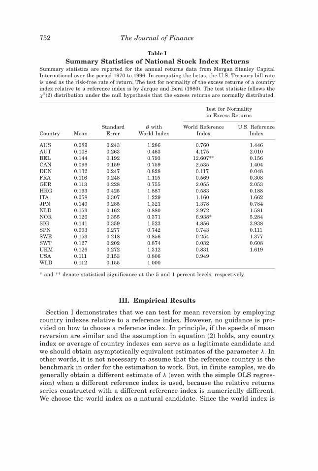

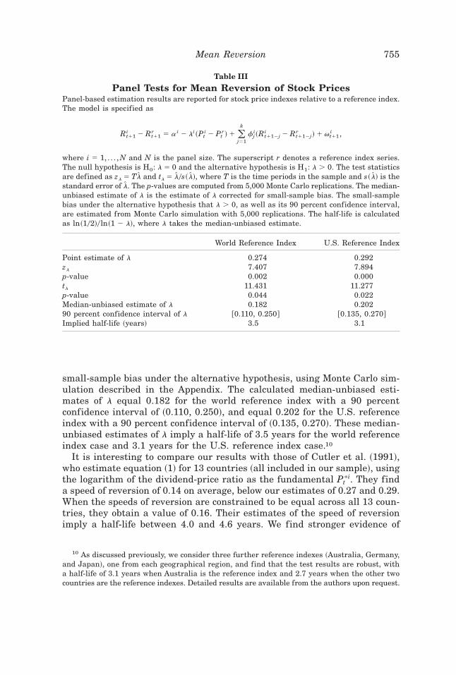


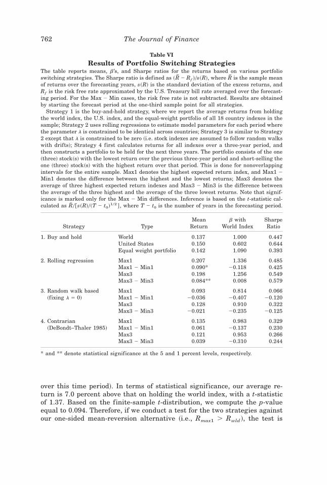

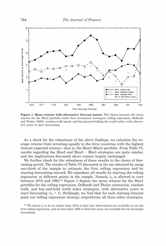


![d ] v€¦ · EPSON Easy Photo Print Photo Print ladi stock DOI ladi stock 002 ladi stock stock ladi stock 005 ladi stock DDE ladi stock 007 stock DDB ladi stock DDS ladi stock 010](https://static.documents.pub/doc/80x56/5f06f3837e708231d41a8cef/d-v-epson-easy-photo-print-photo-print-ladi-stock-doi-ladi-stock-002-ladi-stock.jpg)


