Optical systems may contain a series of various dis-persive optical elements such as mirrors, polarizers,a beam splitter, and lenses. A short pulse propagat-ing through such dispersive optical elements can bedistorted, because different spectral components ofthis pulse accumulate different phases [1].An important characteristic of a dispersive optical
element is group delay (GD) of an optical element,which is defined as the derivative of the spectralphase with respect to the light frequency ω with aminus sign. Group delay dispersion (GDD) is the de-rivative of GD with respect to ω. In order to properlycompensate the phase distortion of an optical pulse,special multilayer coatings can be used [2]. Thesecoatings, called dispersive (or chirped) mirrors,provide high reflection and specific GD and GDDwavelength dependencies in required spectralranges [3–8]. Modern laser techniques, includingfemtosecond laser oscillators [6] and externalenhancement cavities [8], require a few fs2 accuracy
of GDD determination that is not achievable with theexisting approaches.
For decades a number of dispersion measurementdevices, including white-light interferometers(WLIs) were reported [9–12]. WLIs are a powerfultool for measuring the GD wavelength dependenceof optical elements in a broad spectral range[9,10]. Usually the WLI is a Michelson-type interfe-rometer with a broadband light source [9–11,13,14].A typical measurement scheme is as follows. An op-tical element under investigation is placed in thesample arm of the interferometer while the referencearm contains a reference sample with known disper-sion. In the course of the measurement process, thereference sample is moved by a motor, and the lengthof the reference arm is varied. When the referencesample is moved, a spectral intensity distribution(spectral scan) at each motor step position ismonitored and recorded. When all scans arerecorded, the intensity values can be arranged bythe wavelength. A temporal intensity distributioncorresponding to a certain wavelength is called an in-terferogram. GD at each wavelength can be obtainedas an instant corresponding to a center position ofthe interferogram [9,10]. An obvious advantage ofthis measurement scheme is that it enables one to
obtain GD simultaneously for all wavelength valuesgenerated by a white-light source.Intensity values in measured interferograms are
affected by a noise of the light source and by a noiseof the detector. Evidently, determination of centerpositions from noisy interferograms is not a straight-forward task. The problem of extracting GD frominterferometric measurements has been consideredin several works [9–11,13,14]. The most widely usedapproach is the Fourier transform technique[11,13,14]. Results provided by the Fourier transformtechnique are, however, strongly dependent on thenoise in interferometric data. In the case of non-uniformmotion of a stepper motor, the Fourier trans-form technique may fail entirely. Correct processingof data requires the application of preliminarysmoothing procedures, which significantly decreaseswavelength resolution of obtained GD and GDDwavelength dependencies (see Section 5).In this paper we present a recently developed
version of WLI, providing interferometric data anda new algorithm that allows us to perform accurateevaluation of the GD and GDD of dispersive mirrors.In Section 2 we describe in detail our interferometerand the interferometric data that can be obtainedusing this device. In Section 3 we propose a newmod-el for the interferogram description and present anew algorithm for interferometric data processing.The model and algorithm are aimed at overcomingthe instability of interferometric data processing inthe case of noisy measurement data. A special partof the algorithm allows us to solve problems causedby nonuniformity of a stepper motor motion. As a re-sult the new algorithm enables us to evaluate the GDand GDD with high accuracy in the spectral rangefrom 600 to 1100nm. This range is determined notby the algorithm itself, but by hardware components:light sources, detectors, and beam splitter (seeSection 2). In Section 3 we also verify the proposedalgorithm using computationally simulated inter-ferometric data and estimate an accuracy of GDand GDD evaluation that can be achieved by thisalgorithm. In Section 4 we apply the new algorithmto processing simulated experimental data. Anexample of processing of real experimental data isdescribed in Section 5, where we also compare ob-tained results with the results based on the Fouriertransform technique. This comparison clearly illus-trates a high wavelength resolution of the developedmethod.
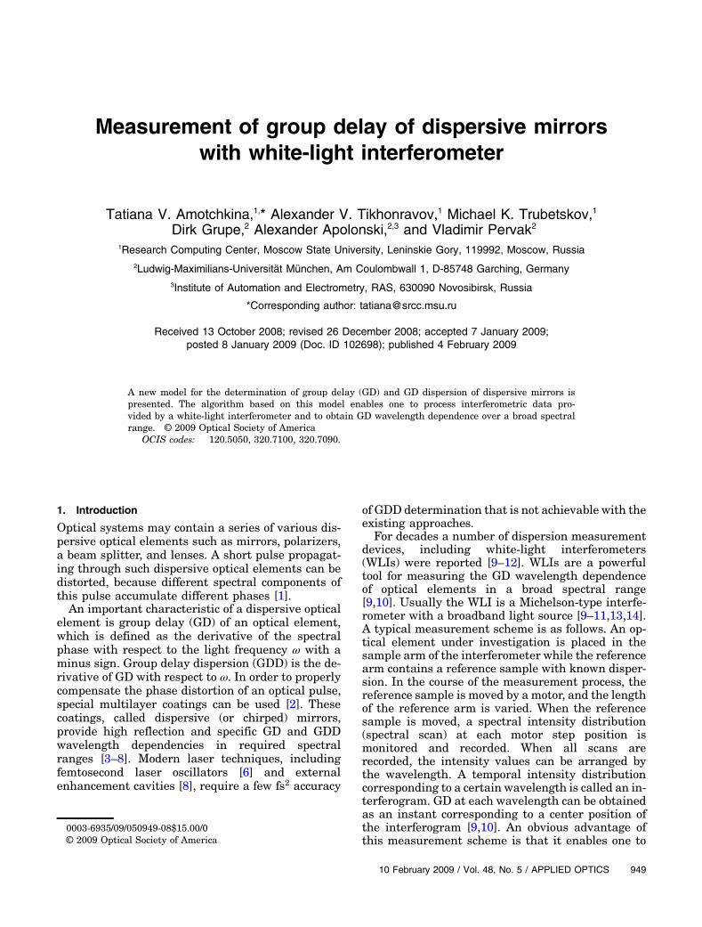
2. Experimental Setup and Initial Interferometric Data
A schematic of our WLI is presented in Fig. 1. Thewavelength grid consists of 1340 spectral points. Afiber-transmitted white light is passed into the inter-ferometer. The incoming collimated beam is dividedby a beam splitter cube into two interferometer arms:sample and reference. The reference arm is movedby a stepper motor that drives a precision lineartranslation stage.
Our motor makes 25 steps per second with a stepsize of 20–30nm. A total scanning time is approxi-mately 8 min. During this time interval, we collect12,000 spectral scans. The exposure time of theCCD camera is less than the interval between adja-cent motor steps. All elements of our WLI are placedon a high-quality optical table, reducing vibrations toan acceptable level.
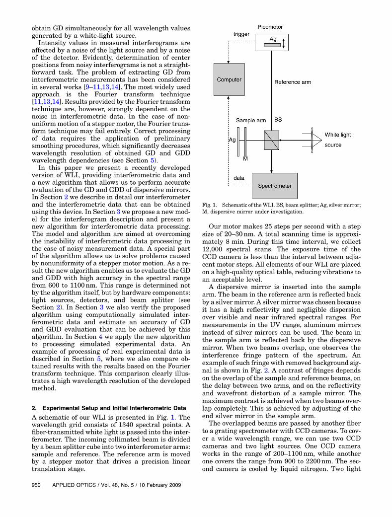
A dispersive mirror is inserted into the samplearm. The beam in the reference arm is reflected backby a silver mirror. A silver mirror was chosen becauseit has a high reflectivity and negligible dispersionover visible and near infrared spectral ranges. Formeasurements in the UV range, aluminum mirrorsinstead of silver mirrors can be used. The beam inthe sample arm is reflected back by the dispersivemirror. When two beams overlap, one observes theinterference fringe pattern of the spectrum. Anexample of such fringe with removed background sig-nal is shown in Fig. 2. A contrast of fringes dependson the overlap of the sample and reference beams, onthe delay between two arms, and on the reflectivityand wavefront distortion of a sample mirror. Themaximum contrast is achieved when two beams over-lap completely. This is achieved by adjusting of theend silver mirror in the sample arm.
The overlapped beams are passed by another fiberto a grating spectrometer with CCD cameras. To cov-er a wide wavelength range, we can use two CCDcameras and two light sources. One CCD cameraworks in the range of 200–1100nm, while anotherone covers the range from 900 to 2200nm. The sec-ond camera is cooled by liquid nitrogen. Two light
Fig. 1. Schematic of theWLI. BS, beam splitter; Ag, silvermirror;M, dispersive mirror under investigation.
sources are a xenon lamp (200–800nm) and a halo-gen lamp (350–2200nm).A computer is used to store data from the spectrom-
eter. One spectral scan is taken at every step of themotor that moves the silver mirror at the end of refer-ence arm. As mentioned earlier, the stepper motormakes 12,000 steps. The background spectral inten-sity distribution, i.e., the intensity distribution with-out interference fringes, is stored and subtracted fromall spectral scans. To obtain the background spectralintensity distribution, one manually translates themotorized stage until fringes disappear completely.As a result of the described measurement process,
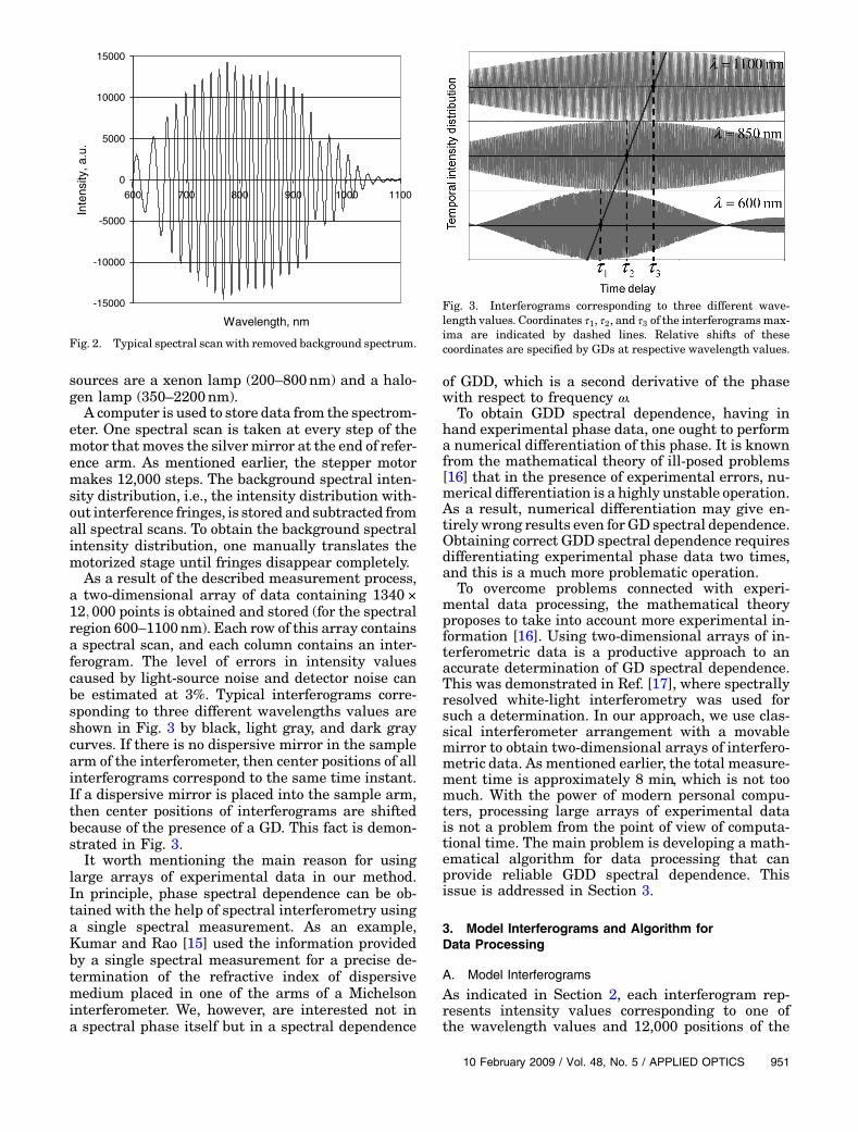
a two-dimensional array of data containing 1340 ×12; 000 points is obtained and stored (for the spectralregion 600–1100nm). Each row of this array containsa spectral scan, and each column contains an inter-ferogram. The level of errors in intensity valuescaused by light-source noise and detector noise canbe estimated at 3%. Typical interferograms corre-sponding to three different wavelengths values areshown in Fig. 3 by black, light gray, and dark graycurves. If there is no dispersive mirror in the samplearm of the interferometer, then center positions of allinterferograms correspond to the same time instant.If a dispersive mirror is placed into the sample arm,then center positions of interferograms are shiftedbecause of the presence of a GD. This fact is demon-strated in Fig. 3.It worth mentioning the main reason for using
large arrays of experimental data in our method.In principle, phase spectral dependence can be ob-tained with the help of spectral interferometry usinga single spectral measurement. As an example,Kumar and Rao [15] used the information providedby a single spectral measurement for a precise de-termination of the refractive index of dispersivemedium placed in one of the arms of a Michelsoninterferometer. We, however, are interested not ina spectral phase itself but in a spectral dependence
of GDD, which is a second derivative of the phasewith respect to frequency ω.
To obtain GDD spectral dependence, having inhand experimental phase data, one ought to performa numerical differentiation of this phase. It is knownfrom the mathematical theory of ill-posed problems[16] that in the presence of experimental errors, nu-merical differentiation is a highly unstable operation.As a result, numerical differentiation may give en-tirelywrong results even forGD spectral dependence.Obtaining correct GDD spectral dependence requiresdifferentiating experimental phase data two times,and this is a much more problematic operation.
To overcome problems connected with experi-mental data processing, the mathematical theoryproposes to take into account more experimental in-formation [16]. Using two-dimensional arrays of in-terferometric data is a productive approach to anaccurate determination of GD spectral dependence.This was demonstrated in Ref. [17], where spectrallyresolved white-light interferometry was used forsuch a determination. In our approach, we use clas-sical interferometer arrangement with a movablemirror to obtain two-dimensional arrays of interfero-metric data. As mentioned earlier, the total measure-ment time is approximately 8 min, which is not toomuch. With the power of modern personal compu-ters, processing large arrays of experimental datais not a problem from the point of view of computa-tional time. The main problem is developing a math-ematical algorithm for data processing that canprovide reliable GDD spectral dependence. Thisissue is addressed in Section 3.
3. Model Interferograms and Algorithm forData Processing
A. Model Interferograms
As indicated in Section 2, each interferogram rep-resents intensity values corresponding to one ofthe wavelength values and 12,000 positions of the
-15000
-10000
-5000
0
5000
10000
15000
600 700 800 900 1000 1100
Wavelength, nm
Inte
nsity
, a.u
.
Fig. 2. Typical spectral scan with removed background spectrum.
Fig. 3. Interferograms corresponding to three different wave-length values. Coordinates τ1, τ2, and τ3 of the interferogramsmax-ima are indicated by dashed lines. Relative shifts of thesecoordinates are specified by GDs at respective wavelength values.
movable mirror in the reference arm. It is commonlyaccepted to plot an interferogram versus a time axiswith the time calculated as a delay of the wave pack-et propagating in the reference arm. We assign t ¼ 0to the first position of the movable mirror. Other co-ordinates on the time axis are calculated as follows:
ti ¼Xi−1k¼1
Δtk; Δtk ¼ 2Δsk=c; ð1Þ
where i is the respective number of the motor stepposition, Δsk is the distance between positions ofthe motor at the kth and ðkþ 1Þth steps, Δtk is thetime increment of wave propagation caused bychanging a motor position between the kth and theðkþ 1Þth steps, and c is light velocity in a vacuum.Equation (1) reflects a real situation in which dis-
tances between adjacent motor positions are not allthe same. Our algorithm of interferogram data pro-cessing requires knowing ti values with sufficient ac-curacy. The algorithm for calculating ti is describedin Subsection 3.C.Intensity values represented by interferograms
correspond to quasi-monochromatic wave packetswith a central wavelength specified by the usedCCD camera. To write down an interferogrammodel,we assume that each wave packet has a rectangularspectrum with a central wavelength λ and a spectralwidth Δλ. In this case, in the absence of a samplemirror, an interferogram is represented by the modelequation (see, for example, Ref. [18]):
IðtÞ ¼ 12IγðtÞ cosωt; ω ¼ 2πc
λ ; ð2Þ
where I is the intensity of the wave packet, c is thelight velocity, and γðtÞ is the envelope function speci-fied by
γðtÞ ¼ sinðΔωt=2ÞΔωt=2 ; Δω ¼ 4πΔλ
λ2 −Δλ2 : ð3Þ
When a dispersive mirror is inserted in the samplearm, Eq. (2) is modified due to a GD caused by a dis-persive mirror and takes the form [18]
IðtÞ ¼ 12Iγðt − τðλÞÞ cosðωtþ αðτÞÞ; ω ¼ 2πc
λ : ð4Þ
Here τðλÞ is a GD at a given wavelength λ, and α is anadditional phase term dependent on a GD. It will beseen that this phase term is not essential for ouralgorithm of data processing. For this reason, wedo not discuss it in more detail.It is seen from Eq. (4) that, in the presence of a
dispersive mirror, a center position of an interfero-gram corresponds to t ¼ τðλÞ. Our algorithm for cal-culating a GD is based on this fact. It is discussed inSubsection 3.B.
B. Data Processing Algorithm
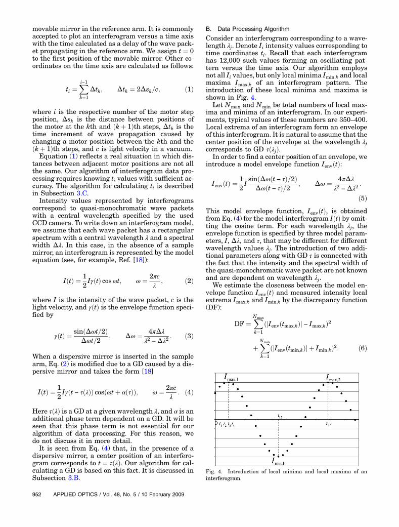
Consider an interferogram corresponding to a wave-length λj. Denote Ii intensity values corresponding totime coordinates ti. Recall that each interferogramhas 12,000 such values forming an oscillating pat-tern versus the time axis. Our algorithm employsnot all Ii values, but only local minima Imin;k and localmaxima Imax;k of an interferogram pattern. Theintroduction of these local minima and maxima isshown in Fig. 4.
Let Nmax and Nmin be total numbers of local max-ima and minima of an interferogram. In our experi-ments, typical values of these numbers are 350–400.Local extrema of an interferogram form an envelopeof this interferogram. It is natural to assume that thecenter position of the envelope at the wavelength λjcorresponds to GD τðλjÞ.
In order to find a center position of an envelope, weintroduce a model envelope function IenvðtÞ:
IenvðtÞ ¼12IsinðΔωðt − τÞ=2Þ
Δωðt − τÞ=2 ; Δω ¼ 4πΔλλ2 −Δλ2 :
ð5ÞThis model envelope function, IenvðtÞ, is obtainedfrom Eq. (4) for the model interferogram IðtÞ by omit-ting the cosine term. For each wavelength λj, theenvelope function is specified by three model param-eters, I, Δλ, and τ, that may be different for differentwavelength values λj. The introduction of two addi-tional parameters along with GD τ is connected withthe fact that the intensity and the spectral width ofthe quasi-monochromatic wave packet are not knownand are dependent on wavelength λj.
We estimate the closeness between the model en-velope function IenvðtÞ and measured intensity localextrema Imax;k and Imin;k by the discrepancy function(DF):
DF ¼XNmax
k¼1
ðjIenvðtmax;kÞj − Imax;kÞ2
þXNmin
k¼1
ðjIenvðtmin;kÞj þ Imin;kÞ2: ð6Þ
Fig. 4. Introduction of local minima and local maxima of aninterferogram.
In Eq. (6), tmax;k and tmin;k are coordinates of the localintensity maxima and minima. These coordinatesare calculated at the preliminary data processingstep described here.Our algorithm is based on the minimization of the
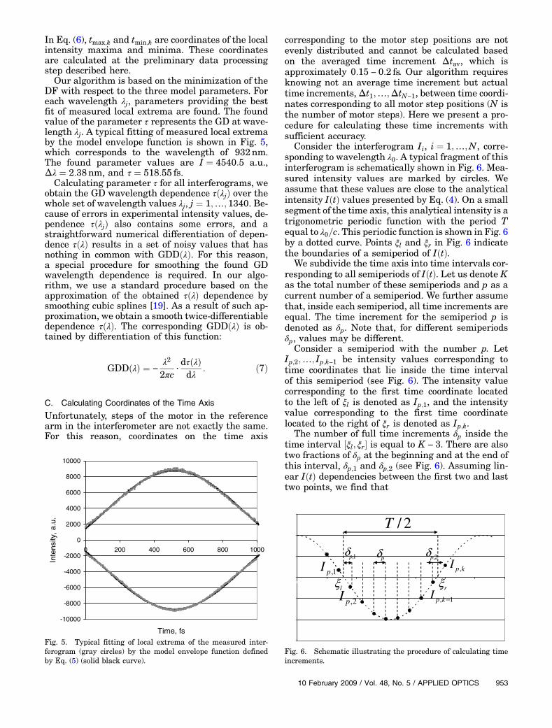
DF with respect to the three model parameters. Foreach wavelength λj, parameters providing the bestfit of measured local extrema are found. The foundvalue of the parameter τ represents the GD at wave-length λj. A typical fitting of measured local extremaby the model envelope function is shown in Fig. 5,which corresponds to the wavelength of 932nm.The found parameter values are I ¼ 4540:5 a.u.,Δλ ¼ 2:38nm, and τ ¼ 518:55 fs.Calculating parameter τ for all interferograms, we
obtain the GD wavelength dependence τðλjÞ over thewhole set of wavelength values λj, j ¼ 1;…; 1340. Be-cause of errors in experimental intensity values, de-pendence τðλjÞ also contains some errors, and astraightforward numerical differentiation of depen-dence τðλÞ results in a set of noisy values that hasnothing in common with GDDðλÞ. For this reason,a special procedure for smoothing the found GDwavelength dependence is required. In our algo-rithm, we use a standard procedure based on theapproximation of the obtained τðλÞ dependence bysmoothing cubic splines [19]. As a result of such ap-proximation, we obtain a smooth twice-differentiabledependence τðλÞ. The corresponding GDDðλÞ is ob-tained by differentiation of this function:
GDDðλÞ ¼ −
λ22πc ·
dτðλÞdλ : ð7Þ
C. Calculating Coordinates of the Time Axis
Unfortunately, steps of the motor in the referencearm in the interferometer are not exactly the same.For this reason, coordinates on the time axis
corresponding to the motor step positions are notevenly distributed and cannot be calculated basedon the averaged time increment Δtav, which isapproximately 0:15 − 0:2 fs. Our algorithm requiresknowing not an average time increment but actualtime increments,Δt1;…;ΔtN−1, between time coordi-nates corresponding to all motor step positions (N isthe number of motor steps). Here we present a pro-cedure for calculating these time increments withsufficient accuracy.
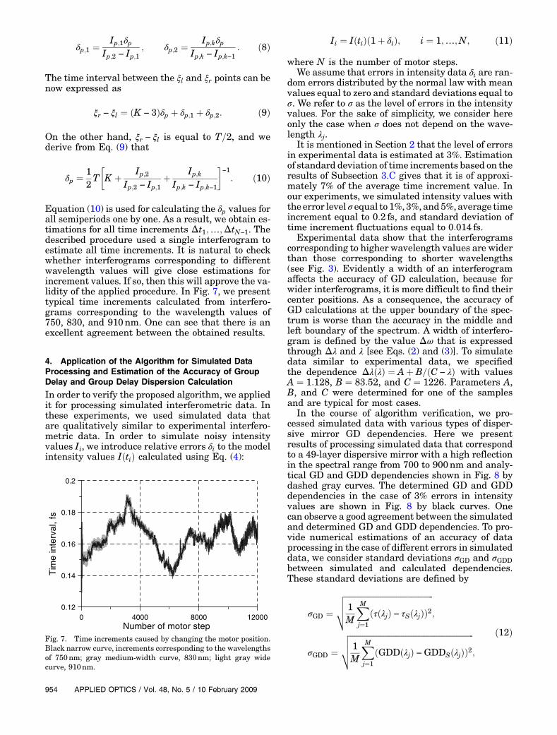
Consider the interferogram Ii, i ¼ 1;…;N, corre-sponding to wavelength λ0. A typical fragment of thisinterferogram is schematically shown in Fig. 6. Mea-sured intensity values are marked by circles. Weassume that these values are close to the analyticalintensity IðtÞ values presented by Eq. (4). On a smallsegment of the time axis, this analytical intensity is atrigonometric periodic function with the period Tequal to λ0=c. This periodic function is shown in Fig. 6by a dotted curve. Points ξl and ξr in Fig. 6 indicatethe boundaries of a semiperiod of IðtÞ.
We subdivide the time axis into time intervals cor-responding to all semiperiods of IðtÞ. Let us denote Kas the total number of these semiperiods and p as acurrent number of a semiperiod. We further assumethat, inside each semiperiod, all time increments areequal. The time increment for the semiperiod p isdenoted as δp. Note that, for different semiperiodsδp, values may be different.
Consider a semiperiod with the number p. LetIp;2;…; Ip;k−1 be intensity values corresponding totime coordinates that lie inside the time intervalof this semiperiod (see Fig. 6). The intensity valuecorresponding to the first time coordinate locatedto the left of ξl is denoted as Ip;1, and the intensityvalue corresponding to the first time coordinatelocated to the right of ξr is denoted as Ip;k.
The number of full time increments δp inside thetime interval ½ξl; ξr� is equal to K − 3. There are alsotwo fractions of δp at the beginning and at the end ofthis interval, δp;1 and δp;2 (see Fig. 6). Assuming lin-ear IðtÞ dependencies between the first two and lasttwo points, we find that
-10000
-8000
-6000
-4000
-2000
0
2000
4000
6000
8000
10000
0 200 400 600 800 1000
Time, fs
Inte
nsity
, a.u
.
Fig. 5. Typical fitting of local extrema of the measured inter-ferogram (gray circles) by the model envelope function definedby Eq. (5) (solid black curve).
-1.5
-1
-0.5
0
0.5
1
1.5
0 1 2 3 4 5 6
lξ rξ,1pI
,2pI , 1p kI −
,p kI
/ 2T
,1pδ ,2pδpδ
Fig. 6. Schematic illustrating the procedure of calculating timeincrements.
The time interval between the ξl and ξr points can benow expressed as
ξr − ξl ¼ ðK − 3Þδp þ δp;1 þ δp;2: ð9Þ
On the other hand, ξr − ξl is equal to T=2, and wederive from Eq. (9) that
δp ¼ 12T
�K þ Ip;2
Ip;2 − Ip;1þ Ip;kIp;k − Ip;k−1
�−1: ð10Þ
Equation (10) is used for calculating the δp values forall semiperiods one by one. As a result, we obtain es-timations for all time increments Δt1;…;ΔtN−1. Thedescribed procedure used a single interferogram toestimate all time increments. It is natural to checkwhether interferograms corresponding to differentwavelength values will give close estimations forincrement values. If so, then this will approve the va-lidity of the applied procedure. In Fig. 7, we presenttypical time increments calculated from interfero-grams corresponding to the wavelength values of750, 830, and 910nm. One can see that there is anexcellent agreement between the obtained results.
4. Application of the Algorithm for Simulated DataProcessing and Estimation of the Accuracy of GroupDelay and Group Delay Dispersion Calculation
In order to verify the proposed algorithm, we appliedit for processing simulated interferometric data. Inthese experiments, we used simulated data thatare qualitatively similar to experimental interfero-metric data. In order to simulate noisy intensityvalues Ii, we introduce relative errors δi to the modelintensity values IðtiÞ calculated using Eq. (4):
Ii ¼ IðtiÞð1þ δiÞ; i ¼ 1;…;N; ð11Þ
where N is the number of motor steps.We assume that errors in intensity data δi are ran-
dom errors distributed by the normal law with meanvalues equal to zero and standard deviations equal toσ. We refer to σ as the level of errors in the intensityvalues. For the sake of simplicity, we consider hereonly the case when σ does not depend on the wave-length λj.
It is mentioned in Section 2 that the level of errorsin experimental data is estimated at 3%. Estimationof standard deviation of time increments based on theresults of Subsection 3.C gives that it is of approxi-mately 7% of the average time increment value. Inour experiments, we simulated intensity values withthe error level σ equal to 1%, 3%, and5%, average timeincrement equal to 0:2 fs, and standard deviation oftime increment fluctuations equal to 0:014 fs.
Experimental data show that the interferogramscorresponding to higher wavelength values are widerthan those corresponding to shorter wavelengths(see Fig. 3). Evidently a width of an interferogramaffects the accuracy of GD calculation, because forwider interferograms, it is more difficult to find theircenter positions. As a consequence, the accuracy ofGD calculations at the upper boundary of the spec-trum is worse than the accuracy in the middle andleft boundary of the spectrum. A width of interfero-gram is defined by the value Δω that is expressedthrough Δλ and λ [see Eqs. (2) and (3)]. To simulatedata similar to experimental data, we specifiedthe dependence ΔλðλÞ ¼ Aþ B=ðC − λÞ with valuesA ¼ 1:128, B ¼ 83:52, and C ¼ 1226. Parameters A,B, and C were determined for one of the samplesand are typical for most cases.
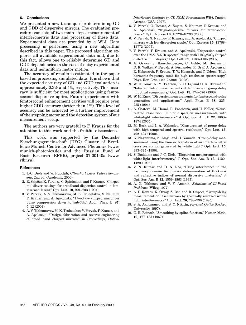
In the course of algorithm verification, we pro-cessed simulated data with various types of disper-sive mirror GD dependencies. Here we presentresults of processing simulated data that correspondto a 49-layer dispersive mirror with a high reflectionin the spectral range from 700 to 900nm and analy-tical GD and GDD dependencies shown in Fig. 8 bydashed gray curves. The determined GD and GDDdependencies in the case of 3% errors in intensityvalues are shown in Fig. 8 by black curves. Onecan observe a good agreement between the simulatedand determined GD and GDD dependencies. To pro-vide numerical estimations of an accuracy of dataprocessing in the case of different errors in simulateddata, we consider standard deviations σGD and σGDDbetween simulated and calculated dependencies.These standard deviations are defined by
Fig. 7. Time increments caused by changing the motor position.Black narrow curve, increments corresponding to the wavelengthsof 750nm; gray medium-width curve, 830nm; light gray widecurve, 910nm.
where τSðλjÞ and GDDSðλjÞ are initial GD and GDDdata, and τðλjÞ and GDDðλjÞ are calculated GD andGDD dependencies. In Table 1, we compare σGDand σGDD values in the cases of 1%, 3%, and 5% errorsin simulated data. These values of σGD and σGDD aretypical for experiments with other simulated GD de-pendencies as well. As mentioned earlier, our experi-mental interferograms have an accuracy of 3%. Thusbased on the results of simulated data processing, wecan expect a relative accuracy of GD calculations ofapproximately 0.3% and a relative accuracy of GDDcalculation of approximately 4%. We determined re-lative accuracy of GD determination as a ratio σGD totypical GD variation in the considered wavelengthrange. For GDD, the relative accuracy is determinedas a ratio of σGDD to a maximum of jGDDj.
5. Application of the Algorithm to ExperimentalData Processing
Here we present results of the application of the no-vel algorithm for experimental data processing. Weconsider a broadband dispersive mirror designedand manufactured for the wavelength range from550 to 1050nm for generating sub-5 fsmJ-levelpulses behind the hollow gas-filled fiber in akilohertz Ti:Sa laser system.In Fig. 9, we present GDD obtained with the help
of the Fourier transform technique (dotted curve)and GDD obtained by the described algorithm (solidcurve). First, one can see that the difference in-creases toward the IR part of spectrum and reachesvalues of 100 fs2. Second, one can conclude thatthe Fourier transform technique provides a GDDwavelength dependence that is significantly over-
smoothed. It happens because the Fourier transformtechnique requires one to preprocess the data pro-vided by the so-called binning procedure thatremoves essential information from interferograms.Our CCD camera provides measurement data at
1340 wavelength points. The binning proceduretakes measurement data at 15 adjacent points andaverages data over these points. Thus the binningprocedure reduces spectral data to approximately100 wavelength points. As a result, the estimatedwavelength resolution of the Fourier transformtechnique is approximately 5nm.
Without preprocessing by the binning procedure,the Fourier transform technique is not able to per-form data evaluation. This is equivalent to a poorwavelength resolution of the Fourier transform tech-nique as compared to the new algorithm. Our novelalgorithm provides a more detailed GDD wavelengthdependence, because during data processing, we takeinto account all information from the WLI. In Fig. 9,we also present a theoretical GDD of this mirror(dashed curve). It is clearly seen that novel approachof WLI data processing provides results much closerto the theoretical GDD wavelength dependence.Extremal values of the GDD are very close, and someshift of the obtained GDD dependence from thetheoretical one is clearly attributed to the presenceof systematic errors in layer thicknesses of thedeposited mirror.
The obtained GD and GDD wavelength dependen-cies can be used for the postproduction characteriza-tion of broadband dispersive mirrors [4]. Using thesedependencies along with spectrophotometric mea-surements allows one to investigate reasons causingdeviations of measured GD and GDD dependenciesfrom the expected ones. This allows one to performcorrections of the manufacturing process in orderto increase a quality of production.
Fig. 8. Comparison of analytical GD and GDD wavelengthdependencies (dashed gray curves) and calculated GD and GDDwavelength dependencies (black curves).
Table 1. Effect of Error Level in Simulated Data on the Accuracyof Group Delay and Group Delay Dispersion Calculation
Error Level σ in Simulated Data (%) 1 3 5
Accuracy of GD Calculation, σGD (fs) 0.05 0.1 0.2Accuracy of GDD Calculation, σGDD (fs2) 1.5 2 3
Fig. 9. GDD obtained from the experimental data by two differ-ent methods: Fourier transform technique (dashed curve) and newalgorithm described in this paper (solid curve). Theoretical GDDdependence of this mirror is shown by dotted curve for comparison.
We presented a new technique for determining GDand GDD of dispersive mirrors. The evaluation pro-cedure consists of two main steps: measurement ofinterferometric data and processing of these data.Experimental data are provided by a WLI. Dataprocessing is performed using a new algorithmdescribed in this paper. The proposed algorithm ex-plores all available experimental data and, due tothis fact, allows one to reliably determine GD andGDD dependencies in the case of noisy experimentaldata and nonuniform motor motion.The accuracy of results is estimated in the paper
based on processing simulated data. It is shown thatthe expected accuracy of GD and GDD evaluation isapproximately 0.3% and 4%, respectively. This accu-racy is sufficient for most applications using femto-second dispersive optics. Future experiments withfemtosecond enhancement cavities will require evenhigher GDD accuracy (better than 1%). This level ofaccuracy can be achieved by a further improvementof the stepping motor and the detection system of ourmeasurement setup.
The authors are very grateful to F. Krausz for theattention to this work and the fruitful discussions.
This work was supported by the DeutscheForschungsgemeinschaft (DFG) Cluster of Excel-lence Munich Centre for Advanced Photonics (www.munich‑photonics.de) and the Russian Fund ofBasic Research (RFBR), project 07-00140a (www.rfbr.ru).
References1. J.-C. Diels and W. Rudolph, Ultrashort Laser Pulse Phenom-
ena, 2nd ed. (Academic, 2006).2. R. Szipöcs, K. Ferencz, C. Spielmann, and F. Krausz, “Chirped
multilayer coatings for broadband dispersion control in fem-tosecond lasers,” Opt. Lett. 19, 201–203 (1994).
3. V. Pervak, A. V. Tikhonravov, M. K. Trubetskov, S. Naumov,F. Krausz, and A. Apolonski, “1.5-octave chirped mirror forpulse compression down to sub-3 fs,” Appl. Phys. B 87,5–12 (2007).
4. A. V. Tikhonravov, M. K. Trubetskov, V. Pervak, F. Krausz, andA. Apolonski, “Design, fabrication and reverse engineeringof broad band chirped mirrors,” in Proceedings, Optical
Interference Coatings on CD-ROM, Presentation WB4, Tucson,Arizona (OSA, 2007).
5. V. Pervak, C. Tiesset, A. Sugita, S. Naumov, F. Krausz, andA. Apolonski, “High-dispersive mirrors for femtosecondlasers,” Opt. Express 16, 10220–10233 (2008).
6. V. Pervak, S. Naumov, F. Krausz, and A. Apolonski, “Chirpedmirrors with low dispersion ripple,” Opt. Express 15, 13768–13772 (2007).
7. V. Pervak, F. Krausz, and A. Apolonski, “Dispersion controlover the UV-VIS-NIR spectral range with HfO2/SiO2 chirpeddielectric multilayers,” Opt. Lett. 32, 1183–1185 (2007).
8. A. Ozawa, J. Rauschenberger, C. Gohle, M. Herrmann,D. R. Walker, V. Pervak, A. Fernandez, R. Graf, A. Apolonski,R. Holzwarth, F. Krausz, T. W. Haensch, and T. Udem, “Highharmonic frequency comb for high resolution spectroscopy,”Phys. Rev. Lett. 100, 253901 (2008).
9. W. H. Knox, N. M. Pearson, K. D. Li, and C. A. Hirlimann,“Interferometric measurements of femtosecond group delayin optical components,” Opt. Lett. 13, 574–576 (1988).
10. W. H. Knox, “Dispersion measurements for femtosecond-pulsegeneration and applications,” Appl. Phys. B 58, 225–235 (1994).
11. A. Gosteva, M. Haiml, R. Paschotta, and U. Keller, “Noise-related resolution limit of dispersion measurements withwhite-light interferometers,” J. Opt. Soc. Am. B 22, 1868–1874 (2005).
12. M. Beck and I. A. Walmsley, “Measurement of group delaywith high temporal and spectral resolution,” Opt. Lett. 15,492–494 (1990).
13. K. Naganuma, K. Mogi, and H. Yamada, “Group-delay mea-surement using the Fourier transform of an interferometriccross correlation generated by white light,” Opt. Lett. 15,393–395 (1990).
14. S. Daddams and J.-C. Diels, “Dispersion measurements withwhite-light interferometry,” J. Opt. Soc. Am. B 13, 1120–1129 (1996).
15. V. N. Kumar and D. N. Rao, “Using interference in thefrequency domain for precise determination of thicknessand refractive indices of normal dispersive materials,” J.Opt. Soc. Am. B 12, 1559–1563 (1995).
16. A. N. Tikhonov and V. Y. Arsenin, Solutions of Ill-PosedProblems (Wiley, 1977).
17. A. P. Kovács, K. Osvay, Z. Bor, and R. Szipöcs, “Group-delaymeasurement on laser mirrors by spectrally resolved white-light interferometry,” Opt. Lett. 20, 788–790 (1995).
18. S. A. Akhomanov and S. Y. Nikitin, Physical Optics (OxfordUniversity, 1997).
19. C. H. Reinsch, “Smoothing by spline function,” Numer. Math.10, 177–183 (1967).