Measurement of internal Strain/Stress Fields by Means of Holography by Carlos Castro Abadía This thesis was submitted as part of the requirement for the MEng. degree in Engineering School of Engineering, Univ. of Aberdeen
Transcript
Measurement of internal Strain/Stress Fields by Means of Holography
by Carlos Castro Abadía
This thesis was submitted as part of the requirement for the MEng. degree in Engineering
School of Engineering, Univ. of Aberdeen
2
Abstract
The goal of the project is the verification of the evaluation method published by
Dändliker. This includes the implementation of his Finite Difference Method as a
computer program as well as the measurement of the surface deformation of an object,
and the determination of the internal stresses and strains. The results of this evaluation
shall be compared with the analytically calculated stresses and strain of the chosen
object. The steps in more details are:
- Implementation of the Dändliker [6] algorithms on a computer. For the
implementation standard software systems may be used, e.g. MatLab.
- Measurement of the bending of a rectangular steel bar under a point load. The steel
bar shall be fixed on one end in the longitudinal direction and the load shall be
applied on the other end, fig. 1.
Fig. 1: Sketch of the set-up
The deformation of the surface shall be measured by Digital Holography in three
dimensions in a sufficient number of surface points.
- The internal stresses and strains shall be evaluated by the Finite Difference Method.
The data must be presented in a form to be compared to an analytical solution.
- The internal stresses and strains shall be evaluated by known analytical solutions.
The two results – measured and computed - for the internal stresses and strains shall be
compared. Differences have to be discussed.
Fsteel bar
3
Contents
1- Introduction 8
1.1- Brief History of Holography 9
1.1.1- Principles of Holography 11
1.1.2- Two mains distributions in Holography 16
1.1.3- In-Plane/Out-of-Plane 16
1.1.4- Non-Destructive Testing 17
1.1.5- Temporal Coherence 18
1.1.6- Spatial Coherence 19
1.1.7- Diffraction 19
1.1.8- Digital Holography 20
1.2- Brief History of the Finite Element Method 22
1.2.1- Finite Elements in Engineering 22
1.2.2- Finite Elements in Mathematics 23
2- Generation Surface Deformation 26
2.1- Selection of the Metal Beam 26
2.2- Application of Finite Element Method 35
3- Dänliker Method 46
3.1- Dänliker Algorithms 46
3.2- Finite Difference 47
3.3- Elasticity Equations 50
3.4- Checking the Dänliker Results 51
4- Set Up in the Holography Lab 53
4.1- Initial Sketch 53
4.2- Improvement of the Sketch 55
4.3- Set Up 60
4.3.1- Utilized Instruments 61
4.3.2- Real Disposition of the Instruments 62
4.3.3- Procedure Explanation 63
4
4.4- Problems Encountered 73
4.5- Results Obtained 74
4.6- Applicable Improvements 74
5- Discussion and Interpretation 75
6- Conclusions 76
7- Recommendations and Suggestions for Future Work 77
8- References 78
9- Appendices 79
9.1- Appendix I. Results of the Nodes in the Finite Element Analysis. 80
9.1.1- Superficial Face 81
9.1.2- Section at 1 mm below the top surface 83
9.1.3- Section at 2 mm below the top surface 86
9.1.4- Section at 3 mm below the top surface 89
9.1.5- Section at 4 mm below the top surface 92
9.1.6- Section at 5 mm below the top surface 95
9.1.7- Section at 6 mm below the top surface 98
9.1.8- Section at 7 mm below the top surface 101
9.1.9- Section at 8 mm below the top surface 104
9.2- Appendix II. Matlab’s Program and Results 107
9.3- Appendix III. Laser Safety 119
5
List of tables and figures
Figure 1.1.2.1 Recording of transmission hologram 13
Figure 1.1.2.2 Scheme of volumetric hologram 14
Figure 1.1.2.3 Recording of reflection hologram 16
Figure 1.1.6.1 Michelson-interferometer 18
Figure 1.1.9.1 Recording a digital hologram 20
Figure 1.1.9.2 Reconstruction with reference wave 21
Figure 1.2.1 Sketch of the metal beam 24
Figure 2.1.1 First disposition of the metal beam 27
Figure 2.1.2 Second disposition of the metal beam 28
Figure 2.1.3 Third disposition of the metal beam 28
Figure 2.1.4 Sketch of the studied system 29
Figure 2.1.5 Plan of the metal beam 31
Figure 2.1.6 Diagram of the metal beam 32
Figure 2.2.1 Distribution of the forces 36
Figure 2.2.2 Types of elements 37
Figure 2.2.3 Mesh of the metal beam 39
Figure 2.2.4 Displacement in X direction 39
Figure 2.2.5 Displacement in Y direction 40
Figure 2.2.6 Displacement in Z direction 40
Figure 2.2.7 Strain in X direction 41
Figure 2.2.8 Strain in Y direction 42
Figure 2.2.9 Strain in Z direction 42
Figure 2.2.10 Stress in X direction 43
Figure 2.2.11 Stress in Y direction 43
Figure 2.2.12 Stress in Z direction 44
Figure 2.2.13 Von Misses Stress 44
Figure 2.2.14 Selected Nodes 45
Figure 3.2.1 Grid in the Finite Difference 48
6
Figure 4.1.1 Initial Sketch 53
Figure 4.1.2 Paths lengths 54
Figure 4.2.1 Description of the Sensitivity Vector 55
Figure 4.2.2 Referent points 56
Figure 4.2.3 Generation of the ellipse 57
Figure 4.2.4 Components of the Sensitivity Vector 57
Figure 4.2.5 Components of the two illumination points 58
Figure 4.2.6 Situation of the points in the metal beam 59
Figure 4.2.7 Improved sketch 60
Figure 4.3.2.1 Detailed sketch 62
Figure 4.3.3.1 Regulation of the laser level 64
Figure 4.3.3.2 Regulation of the speck of the reference beam 64
Figure 4.3.3.3 Regulation of the reference beam level 65
Figure 4.3.3.4 Positive telescopic system 66
Figure 4.3.3.5 Negative telescopic system 67
Figure 4.3.3.6 Regulation of the Defocusing Lend 68
Figure 4.3.3.7 Regulation of the horizontally of the convex lend 68
Figure 4.3.3.8 Regulation of the vertically of the convex lend 69
Figure 4.3.3.9 Regulation of the last beam splitter for the illumination beam 71
Figure 4.3.3.10 Regulation of the last beam splitter for the reference beam 71
Figure 4.3.3.11 Real assembly in the holography lab 1. 72
Figure 4.3.3.12 Real assembly in the holography lab 2. 72
Table 9.1.1.1 Displacement of the Nodes at superficial face 80
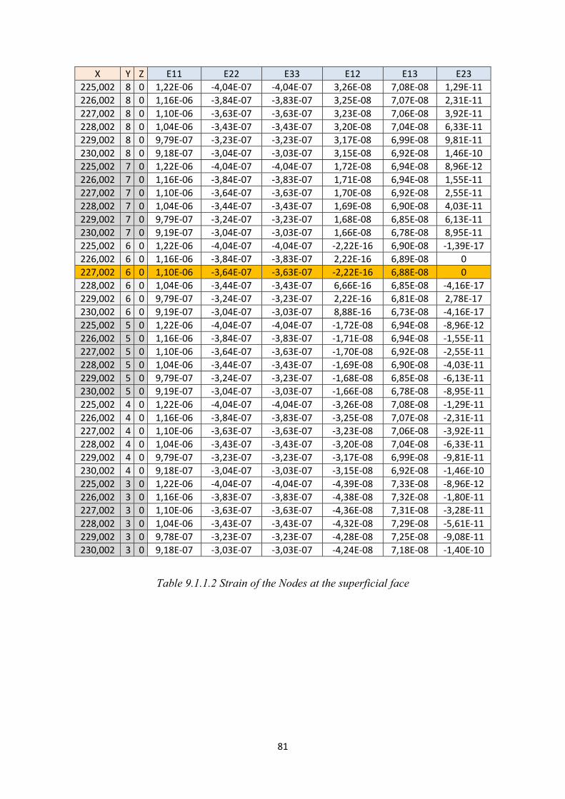
Table 9.1.1.2 Strain of the Nodes at superficial face 81
Table 9.1.1.3 Stress of the Nodes at superficial face 82
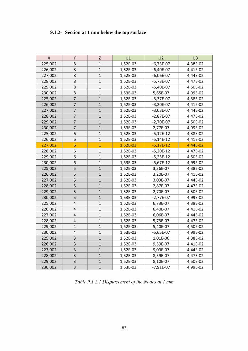
Table 9.1.2.1 Displacement of the Nodes at 1mm 83
Table 9.1.2.2 Strain of the Nodes at 1mm 84
Table 9.1.2.3 Stress of the Nodes at 1 mm 85
Table 9.1.3.1 Displacement of the Nodes at 2 mm 86
Table 9.1.3.2 Strain of the Nodes at 2 mm 87
Table 9.1.3.3 Stress of the Nodes at 2 mm 88
Table 9.1.4.1 Displacement of the Nodes at 3 mm 89
7
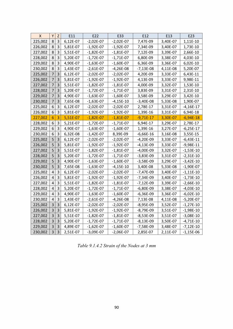
Table 9.1.4.2 Strain of the Nodes at 3 mm 90
Table 9.1.4.3 Stress of the Nodes at 3 mm 91
Table 9.1.5.1 Displacement of the Nodes at 4 mm 92
Table 9.1.5.2 Strain of the Nodes at 4 mm 93
Table 9.1.5.3 Stress of the Nodes at 4 mm 94
Table 9.1.6.1 Displacement of the Nodes at 5 mm 95
Table 9.1.6.2 Strain of the Nodes at 5 mm 96
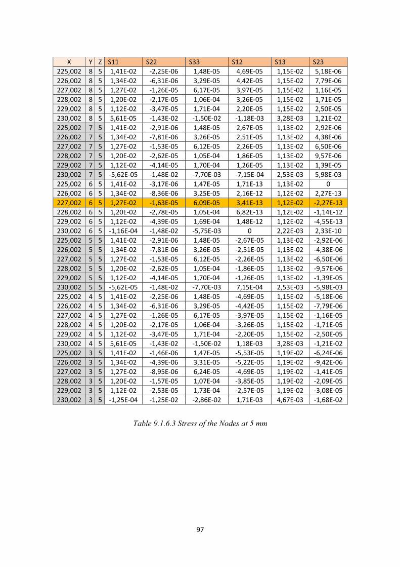
Table 9.1.6.3 Stress of the Nodes at 5mm 97
Table 9.1.7.1 Displacement of the Nodes at 6 mm 98
Table 9.1.7.2 Strain of the Nodes at 6 mm 99
Table 9.1.7.3 Stress of the Nodes at 6 mm 100
Table 9.1.8.1 Displacement of the Nodes at 7 mm 101
Table 9.1.8.2 Strain of the Nodes at 7 mm 102
Table 9.1.8.3 Stress of the Nodes at 7 mm 103
Table 9.1.9.1 Displacement of the Nodes at 8 mm 104
Table 9.1.9.2 Strain of the Nodes at 8 mm 105
Table 9.1.9.3 Stress of the Nodes at 8 mm 106
Table 9.3.1 Classification of the lasers 123
8
1- Introduction
Measurement of internal strain/stress by means of holography is a field really
interesting.
One of the most interesting points is the capacity of measure behaviors of the studied
object without damage the object. This means that it is possible to get important
information without change elastic, plastic or even thermal characteristics of the
material and the object.
It can be possible when it is applied the Non-Destructive Testing (NDT) by Digital
Holography (DH), which mean it is going to be explained afterwards.
This kind of studies are used in aircraft industry like is explained afterwards in the brief
history of the holography.
It is also important the role of the Finite Element Method (FEM) in this study. This
analysis allows check and compares the two results. However, the FEM is not an
exactly method but very approximated as well.
In this project is going to be explain how obtain the strains and stresses inside a metal
beam by Finite Element (a simulation technique very used nowadays by mechanical and
structural companies) by the software of finite elements Abaqus.
Then, the application of the Dänliker algorithms to extrapolate the deformation of the
surface of the metal beam inside it. This equations are really interesting when you only
can obtain the surface displacement, like in holography measurement.
And finally the set up to compare the results of FEM with Digital Holography and
Dänliker algorithms.
Once explained that, it is interesting to understand why these are the methods followed
in this project, doing a brief introduction about the holography (to comprehend Digital
Holography) and FEN; and taking a look of the evolution of this two fields.
9
1.1- Brief History of Holography
Holography dates from 1947, when British (native of Hungary) scientist Dennis Gabor
developed the theory of holography while working to improve the resolution of an
electron microscope. Gabor coined the term hologram from the Greek words holos,
meaning "whole," and gramma, meaning "message". Further development in the field
was stymied during the next decade because light sources available at the time were not
truly "coherent" (monochromatic or one-color, from a single point, and of a single
wavelength).
This barrier was overcome in 1960 by Russian scientists N. Bassov and A. Prokhorov
and American scientist Charles Towns with the invention of the laser, whose pure,
intense light was ideal for making holograms. In that year the pulsed-ruby laser was
developed by Dr. T.H. Maimam. This laser system (unlike the continuous wave laser
normally used in holography) emits a very powerful burst of light that lasts only a few
nanoseconds (a billionth of a second). It effectively freezes movement and makes it
possible to produce holograms of high-speed events, such as a bullet in flight, and of
living subjects. The first hologram of a person was made in 1967, paving the way for a
specialized application of holography: pulsed holographic portraiture.
In 1962 Emmett Leith and Juris Upatnieks of the University of Michigan recognized
from their work in side-reading radar that holography could be used as a 3-D visual
medium. In 1962 they read Gabor's paper and "simply out of curiosity" decided to
duplicate Gabor's technique using the laser and an "off-axis" technique borrowed from
their work in the development of side-reading radar. The result was the first laser
transmission hologram of 3-D objects (a toy train and bird). These transmission
holograms produced images with clarity and realistic depth but required laser light to
view the holographic image. Their pioneering work led to standardization of the
equipment used to make holograms. Today, thousands of laboratories and studios
possess the necessary equipment: a continuous wave laser, optical devices (lens, mirrors
and beam splitters) for directing laser light, a film holder and an isolation table on which
exposures are made. Stability is absolutely essential because movement as small as a
quarter wave- length of light during exposures of a few minutes or even seconds can
10
completely spoil a hologram. The basic off-axis technique that Leith and Upatnieks
developed is still the staple of holographic methodology.
Also in 1962 Dr. Yuri N. Denisyuk from Russia combined holography with 1908 Nobel
Laureate Gabriel Lippmann's work in natural color photography. Denisyuk's approach
produced a white-light reflection hologram which, for the first time, could be viewed in
light from an ordinary incandescent light bulb.
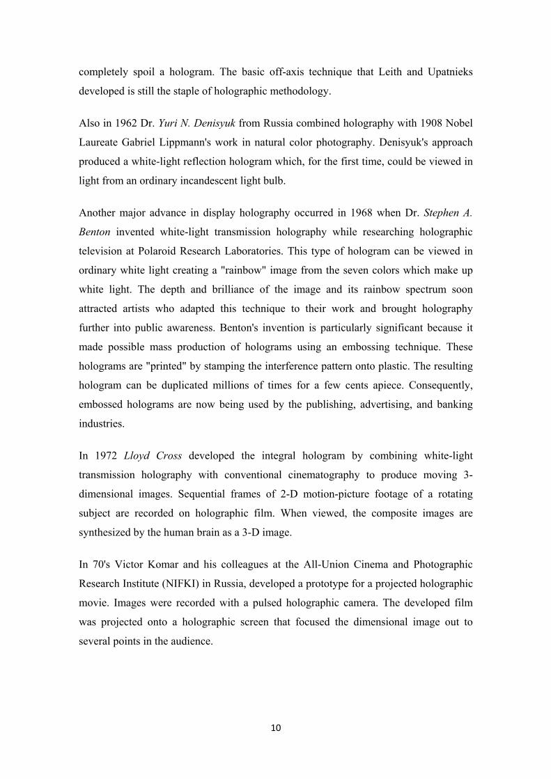
Another major advance in display holography occurred in 1968 when Dr. Stephen A.
Benton invented white-light transmission holography while researching holographic
television at Polaroid Research Laboratories. This type of hologram can be viewed in
ordinary white light creating a "rainbow" image from the seven colors which make up
white light. The depth and brilliance of the image and its rainbow spectrum soon
attracted artists who adapted this technique to their work and brought holography
further into public awareness. Benton's invention is particularly significant because it
made possible mass production of holograms using an embossing technique. These
holograms are "printed" by stamping the interference pattern onto plastic. The resulting
hologram can be duplicated millions of times for a few cents apiece. Consequently,
embossed holograms are now being used by the publishing, advertising, and banking
industries.
In 1972 Lloyd Cross developed the integral hologram by combining white-light
transmission holography with conventional cinematography to produce moving 3-
dimensional images. Sequential frames of 2-D motion-picture footage of a rotating
subject are recorded on holographic film. When viewed, the composite images are
synthesized by the human brain as a 3-D image.
In 70's Victor Komar and his colleagues at the All-Union Cinema and Photographic
Research Institute (NIFKI) in Russia, developed a prototype for a projected holographic
movie. Images were recorded with a pulsed holographic camera. The developed film
was projected onto a holographic screen that focused the dimensional image out to
several points in the audience.
11
Holographic artists have greatly increased their technical knowledge of the discipline
and now contribute to the technology as well as the creative process. The art form has
become international, with major exhibitions being held throughout the world.
1.1.2- Principles of Holography
There are two physical phenomena as the principles of the holography: interference and
diffraction of light waves. Holograms are photographs of three dimensional impressions
on the surface of light waves. Therefore, in order to make a hologram you need to
photograph light waves. This presents something of a dilemma. As we all know, it can
be problematic to take a photograph of a quickly moving object. If you've ever had a
picture come back blurred from the film lab, you know all too well. When a person
moves too quickly in a photograph, their image blurs. Try to imagine the problems
associated with trying to photograph a photon. To start, a light wave moves at the speed
of light. That is about 300.000 kilometers per second. That is more than half way to the
moon in a second. Considerably faster than someone's hand waving. In fact, its so fast
that the very idea of even capturing it on film would appear impossible. What we need
is a way to stop the photon so it can be photographed. And this technique is called
interference.
Imagine yourself standing on a small bridge over of still water. Let’s further imagine
that you were to drop a pebble into the pond. As it hits the water it creates a circular
wave. This wave radiates outwards in an ever growing circular path. We've all done
this. Now, if you drop two pebbles in the water, you would create two circular waves,
each of which would grow in size and eventually cross the path of the other wave and
then continue on its individual expanding path. Where the two circular waves cross each
other, you might say that they interfere with each other. And the pattern that they make
is called an interference pattern. Not too difficult to envision. This is what interference
is. Two waves interfering with each other as they cross paths. No permanent impact is
left on either wave once it leaves the area of overlap. Each wave looks exactly the same
as it did before it crossed the other waves path. Well, maybe it is grown a little bit
bigger, but that's about it. So, what's the big deal about interference in that case?
12
Here it is. As waves cross paths and interfere, the pattern they make is called a standing
wave. It is called a standing wave because it stands still. And since it stands still, it can
be photographed. This solves the problem of how we can photograph something moving
at the speed of light. So, to photograph interference pattern we should use special light
source. It is laser, which was first made to operate in 1960.
Laser light differs drastically from all other light sources, man-made or natural, in one
basic way which leads to several startling characteristics. Laser light can be coherent
light. Ideally, this means that the light being emitted by the laser is of the same
wavelength, and is in phase.
When two light waves pass through each other each wave acts like a bump to the other.
And the result is like rapids of light. The standing wave patterns are stationary even
though the light waves energy continues to move. When waves meet they perform
addition and subtraction. When two waves of equal size meet at their high points (called
crests), they add together to make a wave twice as high at that point. Conversely, where
two waves of equal size meet at their low points (call troughs) they add together to
become twice as low. And when one wave at its high point meets another wave at its
low point they subtract and cancel out. But it isn't really cancelled out in the sense of
being destroyed. Its more a case of there being no light at that spot. If you follow the
wave down its path just a drop further it will be meeting the other wave at a different
relationship and once again be visible. It is a situation of infinite possibilities. Just like
the patterns possible as the waves of two pebbles meet in a pond. At any point you may
notice that the standing wave pattern has produced a place where the waves have added
together to get higher or subtracted to become lower or even just gone flat. There are
few terms that are used to describe the possible encounters. If the waves add and get
higher it is called constructive interference. If the waves subtract or cancel altogether its
called destructive interference.
In holography, there are two basic waves that come together to create the interference
pattern. First and foremost is the wave that bounces off the object we are making a
hologram of. Since it bounces off the object, thereby taking its shape, it is called the
object wave. You can't have interference without something to interfere with. So a
second wave of light that has not bounced off an object is used to perform this function.
It is called the reference wave. When an object wave meets a reference wave creating a
13
standing wave pattern of interference, it is photographed and called a hologram. Semi-
transparent mirror divides laser beam into two beams. The first beam which is called a
signal beam is directed by mirror, expanded by lens and it illuminates object. The
second beam, called a reference beam, is also directed by mirror, expanded by lens and
it falls directly onto photoplate. The photoplate registers an interference pattern between
the bearing beam and the light beam, reflected from the object. A transmission
hologram appears after an ordinary photo-chemical treatment (hologram of Leith-
Upatnieks). If such a hologram is exposed to a laser light beam, you may see a 3-d
image of the object. The transmission hologram does not reconstruct the image in
ordinary white light, and it is necessary to copy it to the reflection hologram.
Figure 1.1.2.1 Recording of transmission hologram [9]
If we write down the hologram in some volumetric medium, the received model of a
standing wave reproduces, for sure, not only amplitude and phase, but also spectral
distribution of the radiation, written down on it. This circumstance was necessary as a
basis of making of the three-dimensional (volumetric) holograms.
As a basis of operation of the volumetric holograms the Bragg's diffraction effect is
used: as a result of an interference of waves, propagating through thick emulsion, the
planes lighted by light of the greater intensity are formed. After processing of the
hologram on the lighted planes the layers of a blackening are formed. As a result of it
14
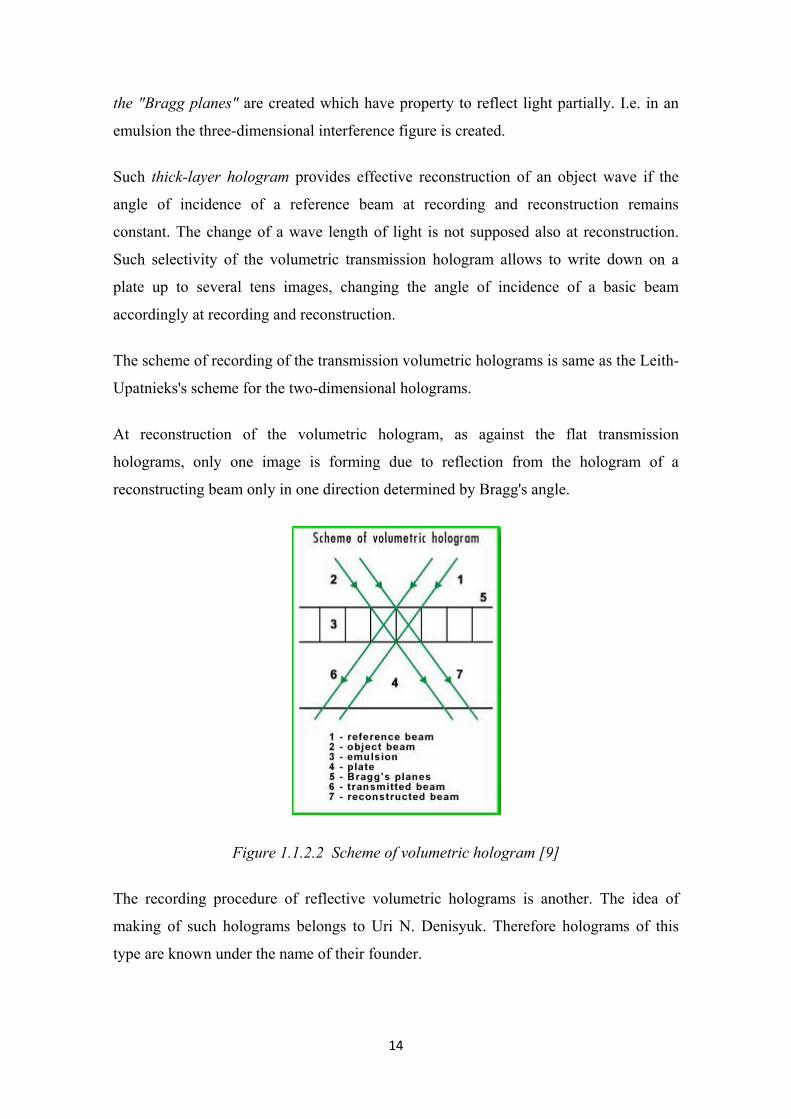
the "Bragg planes" are created which have property to reflect light partially. I.e. in an
emulsion the three-dimensional interference figure is created.
Such thick-layer hologram provides effective reconstruction of an object wave if the
angle of incidence of a reference beam at recording and reconstruction remains
constant. The change of a wave length of light is not supposed also at reconstruction.
Such selectivity of the volumetric transmission hologram allows to write down on a
plate up to several tens images, changing the angle of incidence of a basic beam
accordingly at recording and reconstruction.
The scheme of recording of the transmission volumetric holograms is same as the Leith-
Upatnieks's scheme for the two-dimensional holograms.
At reconstruction of the volumetric hologram, as against the flat transmission
holograms, only one image is forming due to reflection from the hologram of a
reconstructing beam only in one direction determined by Bragg's angle.
Figure 1.1.2.2 Scheme of volumetric hologram [9]
The recording procedure of reflective volumetric holograms is another. The idea of
making of such holograms belongs to Uri N. Denisyuk. Therefore holograms of this
type are known under the name of their founder.
15
The reference and object light beams are formed with the help of a semi-transparent
mirror and directed by a mirror on a plate from two opposite sides. The object wave
shines a photographic plate on the part of an emulsion layer, reference wave - on the
part of a glass substrate. The Bragg's planes in such requirements of recording scheme
almost parallel planes of a photoplate. Thus, the thickness of a photolayer may be rather
small.
On the recording scheme the object wave is formed from the transmission hologram. I.e.
in the beginning usual transmission holograms are made by the technology, described
above, and then make in a copying mode the Denisyuk's holograms from these
holograms (which are termed the master holograms).
The basic property of the reflective holograms is an opportunity of reconstruction of the
image with the help of a source of white light, for example, incandescent bulb or the
Sun. The important property is the colour selectivity of such hologram. It means, that at
the image reconstruction by a white light, it will be restored in colour, that was used
during hologram recording. For example, if ruby laser (red light) was used for recording
procedure, the restored image of the object will be red.
According to property of colour selectivity it is possible to manufacture colour
hologram of the object, exactly reproducing its natural colour. For this purpose it is
necessary to mix three colours at the hologram recording: red, green and blue or to shine
consistently a photoplate by these colours. But, technology of the colour holograms
manufacturing is in an experimental stage and some more efforts and experiments will
be required. It is remarkable, that a lot of people, visitors of exhibitions of the
holograms, usually say, that they can see the colour volumetric images.
16
Figure 1.1.2.3 Recording of reflection hologram [9]
1.1.3- Two mains distributions in holography
Distribution in-line: white light beam and beam reflected by the object are in the same
way or in the same line; it means that the angle between the two beams is 00.
Distribution off-axis: white light beam and beam reflected by the object arrive to the
recording plate with an angle between them.
1.1.4- In-plane/Out-of-plane
One of the most powerful fields in the interferometric optical techniques is the measure
of surface displacement. A point on the surface has a set of local Cartesian co-ordinate
associated with it. The Z axis of this coordinate system is normal to the surface and the
X and Y axes are tangents in the horizontal and vertical directions, respectively. So, “in-
plane” for the local co-ordinate system is the plane tangent to the surface (XY).
An object being viewed by an optical system is located within a global co-ordinate
system. The optical line of sight is usually aligned along the Z axis of the global co-
ordinates, and in-plane sensitivity of the optical instrument refers to the global X-Y
17
plane. Thus, in order to determine local surface in-plane data, the shape of the object
and its orientation in the optical arrangement must be known, and the global in-plane
data must be transformed from one co-ordinate system to the other. Holographic
contouring, as described earlier, is the most expedient means of gathering data for the
co-ordinate transformations.
1.1.5- Non-Destructive Testing
Non-Destructive Testing (NDT) is used to test materials and components without
destruction. NDT methods are applied e.g. in aircraft industry, in power plants and in
automotive production.
Holography Non-Destructive Testing (HNDT) measures the deformation due to
mechanical or thermal loading of a specimen. Flaws inside the material are detected as
an inhomogeneity in the fringe pattern corresponding to the surface deformation.
HNDT can be used wherever the presence of a structural weakness results in a surface
deformation of the stressed component. The load can be realized by the application of a
mechanical force or by a change in pressure or temperature. Holographic NDT indicates
deformations down to the submicrometer range, so loading amplitudes far below any
damage threshold are sufficient to produce detectable fringe patterns [2].
In HNDT it is sufficient to have one fringe pattern of the surface under investigation.
Quantitative evaluation of the displacement vector field is usually not required. The
fringe pattern is evaluated qualitatively by the human observer or, more and more, by
fringe analysis computer codes.
In the field of holography is really important know several concepts and properties
about the light and the waves of a beam light. So, it is very important explain some
concepts like ‘Temporal Coherence’, ‘Spatial Coherence’ and ‘Diffraction’. These
concepts have to be well known for making after the experiment.
18
1.1.6- Temporal Coherence
The Temporal Coherence is explained by the Michelson-interferometer (figure 1.1.6.1).
Figure 1.1.6.1 Michelson-interferometer
Light emitted by the light source S is split into two partial waves by the beam splitter
BS. The partial waves travel to the mirrors M1 respectively M2, and are reflected back
into the incident directions. After passing the beam splitter again they are superimposed
at a screen. Usually the superimposed partial waves are not exactly parallel, but are
interfering with a small angle. As a result a two-dimensional interference pattern
becomes visible.
The optical path length from BS to M1 and back to BS is s1, the optical path length
from BS to M2 and back to BS is s2. Experiments prove that interference can only
occur if the optical path different s1-s2 does not exceed a certain length L. If the
optical path difference exceeds this limit, the interference fringes vanish and just an
uniform brightness becomes visible on the screen. The qualitative explanation for this
19
phenomenon is as follows: Interference fringes can only develop if the superimposed
waves have a well defined phase relation.
The phase difference between waves emitted by different sources varies randomly and
thus the waves do not interfere. The atoms of the light source emit wave trains with
finite length L. If the optical path difference exceeds this wave train length, the partial
waves belonging together do not overlap after passing the different ways and
interference is not possible [1].
1.1.7- Spatial Coherence
Spatial coherence describes the mutual correlation of different parts of the same
wavefront.
Spatial coherence describes also the ability for two points in space, x1 and x2, in the
extent of a wave to interfere, when averaged over time. More precisely, the spatial
coherence is the cross-correlation between two points in a wave for all times. If a wave
has only 1 value of amplitude over an infinite length, it is perfectly spatially coherent.
The range of separation between the two points over which there is significant
interference is called the coherence area, Ac. This is the relevant type of coherence for
the Young’s double-slit interferometer [1].
1.1.8- Diffraction
To explain the phenomenon of Diffraction it is necessary to imagine a light wave which
hits an obstacle. This might be an opaque screen with some transparent holes, or vice
versa, a transparent medium with opaque structures. From geometrical optics it is
known that the shadow becomes visible on a screen behind the obstacle. By closer
examination, one finds that this is not strictly correct. If the dimensions of the obstacle
are in the range of the wavelength, the light distribution is not sharply bounded, but
forms a pattern of dark and bright regions.
Diffraction can be also explained with the Huygens ’ Principle:
20
‘Every point of a wavefront can be considered as a source point for secondary spherical
waves. The wavefront at any other place is the coherent superposition of these
secondary waves.’ [1]
Once done a little review of holography it will be good to do a little review of digital
holography, because the holography that is going to be used is digital holography.
1.1.9- Digital Holography
The concept of digital hologram recording is illustrated in figure 1.1.9.1. A plane
reference wave and the wave reflected from the object are interfering at the surface of a
Charged Coupled Device (CCD). The resulting hologram is electronically recorded and
stored. The object is in general a three dimensional body with diffusely reflecting
surface, located at a distance d as well, but in the opposite direction from the CCD, see
figure 1.1.9.2 [1].
Figure 1.1.9.1 Recording a digital hologram
21
Figure 1.1.9.2 Reconstruction with reference wave
There are several vantages and disadvantages between common holography and digital
holography, and these are the cause of using digital holography in this work [8]:
+ Digital holograms have strong anti-disturb property.
+ They are easy to be modified.
+ They are difficult to be imitated.
+ By using the pixel holograph and embossment, hologram films can be fabricated
by transforming digital holograms. This can make digital hologram anti-
counterfeiting identifiers.
+ Digital holography uses holographic printers, exposing the photosensitive
emulsion with computer generated images. This leads to the creation of
conventional holograms with digital content rather than real scenery.
+ 2D/ 3D graphics or digital photographs and movies can be printed which helps
in the holographic recording of real outdoor scenes, completely synthetic
objects, and objects in motion. This is impossible to achieve with optical
holography.
+ Digital holograms can be multiplexed.
+ Another basic advantage is that the content for digital holograms can easily be
created by non-experts and the printing process is not very expensive compared
to conventional holograms.
22
+ A series of digital photographs or a short movie of a real object is enough for
producing digital holograms.
− Digital holograms lack in the quality in terms of color appearance, resolution,
sharpness, etc. of conventional optical holograms.
− It is really difficult to do digital holography off-axis, because CCD-Camera
needs a very small angle between the two lights beams, so it is better to use in-
line. It means that the resolution increase while the angle between the two beams
decrease.
1.2- Brief history of the Finite Element Method
To understand the progress in Finite Elements it is worthwhile to briefly review the
history of the method, which was developed more or less in parallel in engineering and
mathematics.
1.2.1- Finite Elements in Engineering
The major development in engineering FEM was related to computers. In 1952 a great
effort was made at Boeing to analyze aircraft structures. A procedure was developed,
and appeared in the literature only by 1956 in [Turner et al., 1956]. The method was
essentially based on classical ideas of matrix structural mechanics cast in the framework
of digital computers. In 1961, it was recognized that the FEM is a special version of the
variational approach of Ritz [Ritz, 1909] and Garlerkin [Galerkin, 1915]. By 1964
several aircraft companies had developed their own finite element programs and in 1965
the ASKA program, written by the group under J.H. Argyris, appeared on the market.
The book by Zienkiewicz and Cheung [Zienkiewicz and Cheung, 1967] which appeared
in 1967 stimulated further development and played an important role. In the late 1960s
23
the program NASTRAN written by MacNeal-Schwendler Corporation appeared on the
market. Since then, dozens of various commercial and research codes were written and
are available.
1.2.2- Finite Elements in Mathematics
If the FEM is understood as an approximate method for solving differential equations
utilizing a variational principle and piecewise polynomial approximation, then likely
G.W. Leibnitz (1646-1716) in 1696 was a user of FEM. At the same time L.Euler
(1707-1783) introduced the variational methods with the approximation approach being
essentially the main tool employed for the derivation of the Euler equation. Leibnitz, in
a letter to Johann Bernoulli (1667-1748) [Leibnitz, 1962], addressed the problem of the
brachistochrone, replacing the general descent curve with a piecewise linear curve with
one and two internal nodes, he determined the coordinates of nodal points to achieve the
brachistochrone.
In the nineteenth century the variational approaches were tools for proving the existence
of a solution of differential equations and various discretizations were also used as
mathematical tools. As an example the history of the variational method for solving the
Poisson problem. G.F.B. Riemann (1826-1866) in his 1851 thesis used the variational
principle of energy minimization, which he called the Dirichlet Principle, to prove the
existence of the solution to this problem, essentially assuming that the minimize exists.
L.T.W. Weierstrass (1815-1897) found an essential flaw in Riemann’s argument about
the existence of the minimizer. This error was corrected much later by Hilbert [Hilbert,
1901] using essentially the principles of functional analysis. The use of the variational
method as a tool for obtaining approximate solutions was first proposed by Ritz [Ritz,
1909], and Galerkin [Galerkin, 1915]. Courant touched on the subject of the variational
method in six papers with the last one in 1943 [Courant, 1943] where he explicitly
proposed a piecewise linear function for approximate solution of the Poisson problem
via minimization of the energy. For this reason, the linear element is sometimes called
the Courant element. Courant proposed the method in 1922 [Hurwitz and
Courant,1922], where he gave the proof of existence of the conformal mapping via
minimization of the Dirichlet integral, by employing a sequence of functions, which he
named the minimal sequence, which has the property that the potential energy decreases
24
and converges to the infimum. A long footnote is given on the construction of the
minimal sequence, where subdivision of the domain into triangles and the use of
piecewise linear functions is proposed.
There are many other instances of discovery of the FEM.
The history of FEM shows that it originated from different sources and today it is a very
mature method where engineering, mathematics, and computer science are interwoven.
On the other hand, the number and richness of the results are so large that it is hard for a
single person to comprehend it. This has led to the development of various specialties
concentrating only on a few particular aspects. For example, focusing on the
computational aspect leads one to emphasize only ‘recipes’ whilst neglecting ideas
behind them, while concentrating on mathematical aspects leads sometimes one to lose
sight of the purpose of FEM, which is the computational analysis of engineering
problems. Focusing on the computer-science aspects, such as the parallelization of FEM
computations, also leads to one sided view.
Once explained a brief summary of the history of the finite element method it is
important to know that the study of the metal beam can be approximated by a two-
dimensional analysis. It means that the deformation of the metal beam can be studied as
if it was a problem of a planar body.
This study will be done in a section of the bar parallel to the direction of the forces.
Figure 1.2.1 Sketch of the metal beam
25
However, in my case it is necessary to do a three-dimensional analysis because it is
essential knowing the behavior of several points in the surface perpendicular to the
direction of the applied force.
Knowing this it is important to do a brief summary of the finite elements for three-
dimensional analysis.
Thus, the fundamental ideas governing the development of element properties for three-
dimensional analysis are unchanged respect two-dimensional analysis; and some
families of elements for three-dimensional analysis are logical extensions of the families
of elements for two-dimensional analysis.
For example, the triangle and rectangle of two-dimensional analysis become the
tetrahedron and rectangular hexahedron respectively of the three-dimensional analysis.
With regard to three-dimensional finite-element analysis it is perhaps appropriate at the
very beginning to emphasize the effect that increasing the number of dimensions has on
the size of a problem (i. e. on the total number of degrees of freedom of the problem).
For example, imagine that in a one-dimensional analysis it is necessary to use n nodes
(at which u is the degree of freedom) to achieve a satisfactory level of accuracy of
solution, i.e. n unknowns are required. Then, for a similar level of accuracy in two-
dimensional analysis we would need to use around n2 nodes with u and v as degrees of
freedom at each node, giving a total of about 2n2 unknowns. Proceeding to three
dimensions we would use about n3 nodes with u, v and w as degrees of freedom for the
same sort of accuracy, giving a total of about 3n3 unknowns. If n=10, say, the necessary
degrees of freedom increase from 10 to 200 to 3000 as we proceed from one to two to
three dimensions. It is clear that the finite-element analysis of practical three-
dimensional solids will often result in the generation of very large numbers of equations
[3].
26
2- Generation Surface Deformation
2.1- Selection of the Metal Beam
To generate the deformed surface is necessary knowing which are going to be the
dimensions, the material and the properties of the bar.
All this things are explained in the text which is below. In this part, some possibilities
have been considered, like the disposition of the metal beam in the lab and in which
way it is going to be clamped, roughly deformation of the extreme of the bar and
selection of the dimensions of the metal beam.
First of all, it is necessary to decide the dimensions of the bar and the material.
Well, there are mainly two options in the field related with the material choice. One
choice is using Steel and another choice is Aluminum Alloy.
Like you can use both of these materials in applications of holography, I’ve chosen
Aluminum Alloy, because its Young’s Modulus is lower, so for the same force applied
the deformation will be bigger, and then the study will be more intuitive.
For deciding the dimensions of the bar I have calculated some the deformations with a
different sections of the bar, so at the end, I can decide more or less which has to be the
definitively section of the bar.
To calculate this deformation, first we have to talk about the disposition of the bar in the
experiment or in which way the bar will be hold.
At the beginning, I thought in only leaning the bar by the two extremes. This idea is
drawn in the figure 2.1.1.
27
Figure 2.1.1 First disposition of the metal beam
This disposition is really good to calculate the deformation in the middle, but the main
problem which did that I couldn’t choose this disposition was the holders, because of
the bar slips when I applied the force.
Then I thought of using the same disposition but using two clamps instead of using two
supports.
28
Figure 2.1.2 Second disposition of the metal beam
The problem of using this layout is that I needed a bar which a length twice to obtain the
deformation that I wish. For this reason, I have taken the last one disposition.
Figure 2.1.3 Third disposition of the metal beam
29
To demonstrate that we need a longer bar if we used the second disposition instead
using the third disposition, we need to use differential equations related with the field of
the elasticity [5].
So, the sketch of the system is:
Figure 2.1.4 Sketch of the studied system
Explication of the letters:
X: Horizontal Displacement. X=0 is at the beginning of the bar.
2L: Length of the bar.
F: Force applied in the middle of the bar.
E: Young’s Modulus
I: Inertia of the bar.
So, if I call:
W: vertical displacement.
W’: angle turned and also means the first derivate.
M: moment in the restriction.
Q: charge or force applied in this point.
30
In this way, we know different things related with the displacement in the clamps.
W=0
W’=0
M≠0
Q≠0
And the differential equation is:
′′ (2.1)
So, the equation is integrated twice we can obtain the vertical displacement depending
in the length of the bar:
′ 1 (2.2)
1 2 (2.3)
Now, if is applied the boundary conditions explained some lines ago, it is possible to
obtain the definitively equation.
0 (2.4)
2 (2.5)
′ 0 0 1 1 0 (2.6)
0 0 2 2 0 (2.7)
And the final equation is:
(2.8)
31
So, if we have to obtain the same maximal deformation, the length of the bar in the
second disposition has to be twice the third disposition, because of in the second
disposition the X will be in the middle of the bar and in the third disposition the X will
be in the extreme of the bar.
Now, I know how to calculate the deformation approximately it is possible to choose
the final section of the bar.
Here it is shown the different possibilities of the dimensions of the bar.
I think that it will be good obtaining a high displacement, because it is more visual that
if the displacement was small.
So, I’ve done the calculations with different thickness, high and length.
So, the dimensions of the bar will be:
a= length
b= thickness
c= height
Figure 2.1.5 Plan of the metal beam
The material chosen is Aluminum Alloy 2014-T6.
For this material de Young Modulus is 69GPa = 69000Pa/mm2 = 69 MPa.
Now, for calculating the inertia and to put in a right way the axis is necessary to show it
in a sketch:
32
Figure 2.1.6 Diagram of the metal beam
So, the inertia will be respected axis X:
(2.9)
In this way, applying the equation of the deformation and the different parameters
written before it is obtained:
(2.10)
(2.11)
(2.12)
33
I’ve done the calculations for different forces and dimensions which are:
• F=100N >>>>>>>> Deformation at the end of the bar = 0,3865 mm
a=150mm
b=15mm
c=15mm
• F=150N >>>>>>>> Deformation at the end of the bar = 0,5791 mm
a=150mm
b=15mm
c=15mm
• F=150N >>>>>>>> Deformation at the end of the bar = 2,12296 mm
a=150mm
b=8mm
c=12mm
• F=150N >>>>>>>> Deformation at the end of the bar = 4,77664 mm
a=150mm
b=12mm
c=8mm
• F=250N >>>>>>>> Deformation at the end of the bar = 7,9611 mm
a=150mm
b=12mm
c=8mm
• F=250N >>>>>>>> Deformation at the end of the bar = 0,96618mm
a=150mm
b=15mm
c=15mm
• F=250N >>>>>>>> Deformation at the end of the bar = 2,3588mm
a=150mm
b=12mm
c=12mm
34
Once I’ve done these calculations, I think that it will be good to take a bar with
thickness between 8mm and 15 mm, and with a height of 8mm and 15mm.
By other hand, I think that I will only need 150mm to do the experiment but I will also
need more length to hold this bar; so I think that it is a good idea take a bar of 300 mm.
Note: The dimensions of the bar are not really important in this project because the
main point is measuring its displacement.
Material: Aluminum Alloy 2014-T6
Length = a = 300mm
Area of the bar could be (b*c)= 12x12, 10x12, 8x10, 10x8, etc.
At the end, it was available in the workshop a bar made of Aluminum Alloy 2014-T6
with the next dimensions:
Length= 300mm
Section of the bar=12x12mm
So, in this way to appreciate in a right way the vertical displacement I am taking the
next dimensions:
200
12
12
150
And using the equation of the vertical displacement at the extreme of the bar it is
possible to approximate the maximum displacement at:
3,3548
35
2.2- Application of Finite Element Method
Once decided the exactly dimensions it is time to assembly the bar in the lab.
Like it is going to be explained in the point of Digital Holography, I need to study the
perpendicular face to the table of the lab of the metal beam; so it is necessary to change
a little the way of applying the force.
So the procedure it is going to be the next:
The direction of the force is going to be parallel to the workbench, it means that the
force will have a horizontally direction.
Nevertheless, it is important applying one of the main properties of the holography
which is the non-destructive testing. It is important to take into account this because it
guarantees that the metal beam doesn’t suffer any kind of permanent deformation.
One explained all these things; it is really important explaining the most important
points of the procedure in the generation of the surface.
So, the software used in this part is Abaqus 6.8.
In this program the coordinate system has changed some components respect the initial
components described upper. So, the next figure shows how it is placed the bar in the
space and the direction of the applied forces.
36
Figure 2.2.1 Distribution of the forces
The reason why I have chosen two concentrated forces is because it simulates the
behavior of the clamp which does the force to the bar.
This is going to be explained in detail in the next chapters, especially in which it is
explained the assembly in the lab.
As I mentioned before about non-destructive testing I will do a maximum deformation
in the extreme of the metal beam about 50 μm.
So, knowing the deformation at the extreme is easy to obtain the necessary force
applied.
(2.13)
0,05 (2.14)
, 1,2161 (2.15)
37
As I am going to apply the force in two concentrated points, the force in each node will
be:
0,608 (2.16)
Once decided the magnitude of the force it is important and necessary knowing which
kind of finite element is going to be applied in the bar.
As I have explained in the introduction of Finite Element Method there are several types
of finite element, depending which analysis you are doing.
In this case, the software Abacus has mainly six types of element, which are for each
kind of analysis.
So, the next picture shows these elements.
Figure 2.2.2 Types of elements [4]
38
In my analysis I have chosen the Hexahedra because it is the most appropriate to realize
a analysis of an object which sections are rectangular.
The rectangular hexahedral element is obviously the three-dimensional element
equivalent of the basic rectangular element in two-dimensions. The element has a total
of 24 degrees of freedom (the nodal freedom are u, v and, w at eight corner nodes) and
the co-ordinate origin is taken for convenience to be at the centroid of the body.
In assuming a displacement field for the element it is natural to begin by considering
expressions for each of u, v, and w as products of linear functions in x, in y, and in z, i.e.
as expressions of the form:
(2.17)
where , , etc. are constants. Multiplying this out gives expressions of the form [3]:
. (2.18)
Once shown this, it is clearer how Abaqus works with this element; so if the number of
element is very huge the computer will have problems to solve the job.
Once selected the type of the element is time to choose the size of the element.
I would like to put the element’s size as small as possible, but if the size is so small the
software has problems to simulate. So, the final and minimum size chosen is 1 mm.
Thus, the metal beam looks like this:
39
Figure 2.2.3 Mesh of the metal beam
At the end, the whole metal beam has been meshed with a total of 35280 elements.
Once meshed the metal beam and submitted and run the job; everything is ready to
obtain the different results.
So, the displacement of every node of the bar in the X, Y and Z directions will be like
the next figures show.
Figure 2.2.4 Displacement in X direction
40
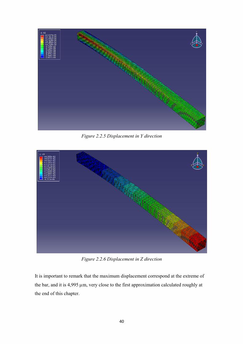
Figure 2.2.5 Displacement in Y direction
Figure 2.2.6 Displacement in Z direction
It is important to remark that the maximum displacement correspond at the extreme of
the bar, and it is 4,995 μm, very close to the first approximation calculated roughly at
the end of this chapter.
41
This small difference can be due to errors of the finite element and the software.
Nevertheless, the numerical approximation is an approximation, it means that it is not
an exactly calculation.
By other hand, the strains in the mains directions are:
Figure 2.2.7 Strain in X direction
42
Figure 2.2.8 Strain in Y direction
Figure 2.2.9 Strain in Z direction
43
And finally the stresses in the mains direction and the Von Misses stress are:
Figure 2.2.10 Stress in X direction
Figure 2.2.11 Stress in Y direction
44
Figure 2.2.12 Stress in Z direction
Figure 2.2.13 Von Misses Stress
All these images represent the whole metal beam. However it is interesting knowing the
displacement in some particular nodes.
45
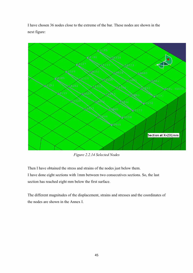
I have chosen 36 nodes close to the extreme of the bar. These nodes are shown in the
next figure:
Figure 2.2.14 Selected Nodes
Then I have obtained the stress and strains of the nodes just below them.
I have done eight sections with 1mm between two consecutives sections. So, the last
section has reached eight mm below the first surface.
The different magnitudes of the displacement, strains and stresses and the coordinates of
the nodes are shown in the Annex I.
46
3- Dänliker Method
3.1- Dänliker Algorithms [6]
It is well known that holographic interferometry allows determining the displacement
field on the surface of solid objects under mechanical load.
It is the purpose of this paper to show that the strain and stress field can be extrapolated
below the surface from the measurable displacements of the surface. This will be
verified, at least for isotropic elastic materials, following Hooke’s law.
To calculate the strains and stresses inside the metal beam, it is necessary first knowing
the way in which the information will be obtain and in which way it will be processed.
So, the differential deformation of the material are completely described by the vector
gradient
, (3.1)
of the displacement field u(x).
It is assumed that μik is completely known in a plane (x, y, z) where z is constant.
So the linear extrapolation in a plane which normal vector is parallel to axis z is possible
through
, , , , , , , (3.2)
if the derivates μik,z = δμik/δz to the plane are known. However, μik,z cannot be directly
calculated, since only the in-plane derivatives μik,α (α=1,2), are accessible from the
given distribution μik in the plane (x, y, z) where z is constant.
The additional relations to determine the nine components of μik,z are given by the
mathematical compatibility conditions
, , (3.3)
47
where i = x, y, z and α = x, y.
The remaining three components of μik,z are found to be explicitly
, , , , , , (3.4)
, , , , , , (3.5)
, , , , , , , (3.6)
As I said in the introduction of the report, the holography system applied is Non-
Destructive System, so the deformation is almost inappreciable and consequently the
curved surface is depreciable and then it is not necessary to rotate the base in which are
placed all the points.
3.2- Finite Difference
Once explained how obtain the derivates of each displacement it is necessary knowing
how obtain the information.
So, the information will be done with the coordinates of the point and the displacement:
Point A: PA= (225; 5; 0) Displacement PA: U = 0.00181923 mm V = -0.000000403692 mm W = 0.0437715 mm To apply this numbers to the equations explained before it is necessary use Finite Difference. This method is a numerical way of doing differentiation. In the Finite Difference there are three possible ways of calculating this differentiation: forward, backward and central. Before explaining each of them it is important remark that the points are going to be operates like they were points of a gird. In which the horizontal distance (ΔX) and vertical distance (ΔY) between points are h. In the next figure is shown the grid with the distributions of the points that will be used for the application of Dänliker algorithms.
48
Figure 3.2.1 Grid in the Finite Difference Forward In this case are used two consecutive points, but it is calculated the first one.
(3.7) Backward In this case are used two consecutive points too; but it is also calculated the first one.
(3.8) Central
In this case are used two non consecutive points, and it is calculated the point between
them.
(3.9)
49
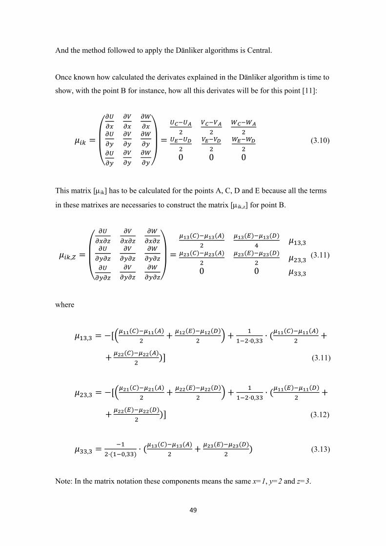
And the method followed to apply the Dänliker algorithms is Central.
Once known how calculated the derivates explained in the Dänliker algorithm is time to
show, with the point B for instance, how all this derivates will be for this point [11]:
0 0 0
(3.10)
This matrix [μik] has to be calculated for the points A, C, D and E because all the terms
in these matrixes are necessaries to construct the matrix [μik,z] for point B.
,
,
,
0 0 ,
(3.11)
where
, ,
(3.11)
, ,
(3.12)
, , (3.13)
Note: In the matrix notation these components means the same x=1, y=2 and z=3.
50
And now, applying the equation 3.2 is possible to obtain the matrix [μik] and [μik,z] in
each of the sections wanted in z direction.
3.3- Elasticity Equations
In this moment, well known these two matrixes are possible to apply the elasticity
equations to obtain the different strains and stresses.
Strain tensor:
(3.14)
where
(3.15)
(3.16)
(3.17)
(3.18)
(3.19)
(3.20)
Stress tensor:
(3.21)
51
where [σ] is symmetric and
11
1
0 0 00 0 00 0 0
0 0 00 0 00 0 0
0 0
0 0
0 0
(3.22)
The Matlab’s program and the results for one point are in appendix II.
3.4- Checking the Dänliker Results.
Now, it is important knowing if the extrapolation is well done.
To know this, it is necessary calculating the matrix of first derivates in a section
(knowing the displacements in this section) and then compares the new principle
components of the strain tensor (ε11’ and ε22’) with the extrapolated components in this
section (ε111 and ε122). Here, the high in the extrapolation that I have taken is h = 1mm,
so it is the section 1.
The method followed to obtain these two components is similar to the method done
before.
Now, it is only necessary four points (A, B, C and D) to calculate the matrix [μik] for the
point B which is in the middle of these points.
It is important to know that all the points and their displacements have been taken in the
section situated at 1 mm below the top surface.
This new program and its results are also in the appendix II.
52
Now, to compare these two results is necessary to calculate the relative error.
(9.1)
Thus, for ε11 and ε22 the error will be respectively:
1 . . .
100 41,3% (9.2)
1 . . .
100 36,41% (9.3)
The big errors are due to the thin difference between the numbers of the matrix E1for
the first algorithm and E0 for the second algorithm (see in appendix II) are really near.
However, some cases which are near but changing the magnitude orders. It does that the
error will be so huge.
It is also important remark that an increment of 1 mm between points it is really big for
using Finite Difference; because Finite Difference is an approximation of the integral
for single points.
All these aspects do that the results were a bit different, but if the increment is smaller
the new results will be nearer.
53
4- Set up in the Holography Lab
4.1- Initial Sketch
Before going to the lab is necessary to know how to put the different devices in the table
of the lab.
The most important things that I must have in my mind are the security and the sketch
of the table of the lab to execute the experiment.
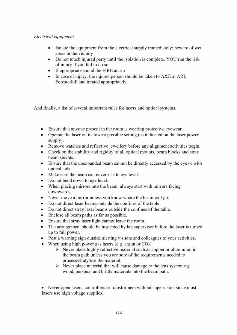
So, the security rules followed in the lab are explained in the Annex II.
The first sketch of the experiment will be like the picture shown in the next figures.
In this first picture it is possible to identify the different components that I will use in
the experiment.
Figure 4.1.1 Initial Sketch
In this second picture, it is to identify the lengths that are necessary to control in the
experiment.
54
It is due to the Temporal Coherence; so the sums of the different ways for the reference
wave and the illumination wave have to be more or less the same.
It means that the whole distance ran for the reference wave has to be the same that the
distance ran for the illumination wave.
1 2 3 1 2 3
Where 1,2,3 is the distance rans in each piece of the way of the
reference wave, and 1,2,3 is the distance ran in each piece of the way of
the illumination wave.
Figure 4.1.2 Paths lengths
55
4.2- Improvement of the Sketch
As the objective of the experiment is measuring the displacement of the bar, it is
necessary take into account several important aspects.
First of all, it is necessary to remember which directions affect in the movement of the
object in holography.
So, if it is drew an Illumination Point (IP) and an Observation Point (OP), both two are
the focus of an ellipse. So, if you move the object through this ellipse there is no
changes in the image taken by holography.
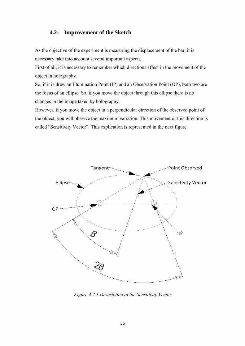
However, if you move the object in a perpendicular direction of the observed point of
the object, you will observe the maximum variation. This movement or this direction is
called “Sensitivity Vector”. This explication is represented in the next figure.
Figure 4.2.1 Description of the Sensitivity Vector
56
So, knowing this now, it is possible to improve the sketch of the experiment and apply
this to the practical. This means that it is necessary to apply the force to the beam in the
horizontal direction (axis X), so we will obtain the displacement in the direction of the
observation direction.
As, I will see the Sensitivity Vector with a certain angle, I need to use two illuminations
points to see the two components of this vector.
So, I will illuminate the metal beam from the right and the left of the observe point, it
means from both sides of the CCD Camera.
The theoretical explanation is the next:
When you want an illumination point and an observation point both respected a
determinate point or studied point or observed point; there is a way or field trough the
observed point can be removed and nothing suffer any kind of change. It is due to the
definition of the ellipse.
′ ′ 0 (4.1)
This is represented in the next two figures; the letter with accent means that is the
displacement vector after the movement.
Figure 4.2.2 Referent points
57
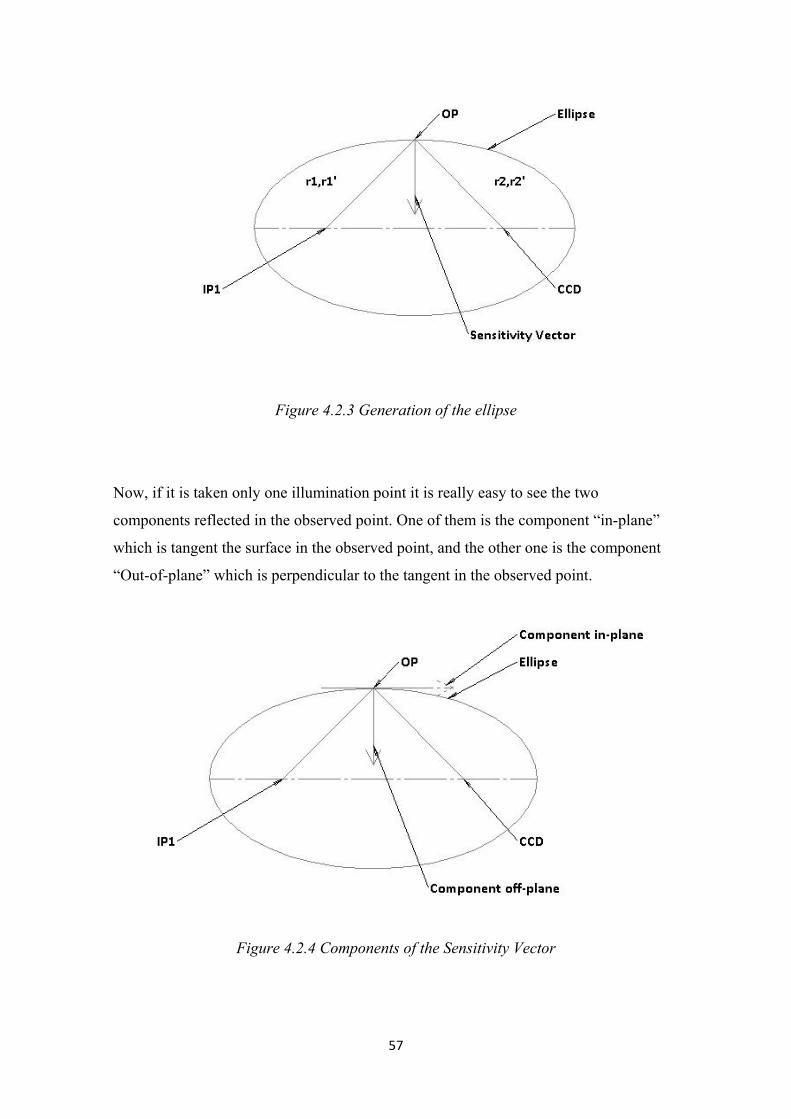
Figure 4.2.3 Generation of the ellipse
Now, if it is taken only one illumination point it is really easy to see the two
components reflected in the observed point. One of them is the component “in-plane”
which is tangent the surface in the observed point, and the other one is the component
“Out-of-plane” which is perpendicular to the tangent in the observed point.
Figure 4.2.4 Components of the Sensitivity Vector
58
So, if we put two illumination points for the same observed point it will be obtained the
next four vectors; two of them are the components “Out-of-plane” (one for each
illumination point) which have the same value and the same direction and orientation.
Otherwise, the components “in-plane” will have the same value and direction but
opposite orientation.
So, at the end it will be obtained only one vector in the direction perpendicular to the
observed point.
Figure 4.2.5 Components of the two illumination points
So, this is the reason why is necessary to use two illumination points; because it is
fundamental to obtain the component “Out-of-plane” to obtain the final displacement by
digital holography.
59
Once explained this, the surface of the metal beam that will be studied is going to
change.
If we take as reference plane a plane parallel situated around 24 cm of the top of the
table, nevertheless the camera is going to record in a horizontal and parallel line from
the surface of the table. So the surface of the metal beam that is going to be observed is
perpendicular to the table. This is shown in the next figure.
Figure 4.2.6 Situation of the points in the metal beam
Now, it is necessary to vary the initial sketch because a new illumination point has to be
introduced.
So, in the next figure is shown the final sketch in the lab.
60
Figure 4.2.7 Improved sketch
4.3- Set Up
Now, that it is known which diagram is going to be followed in the lab it is necessary to
name and explain the different devices that will be used, the real disposition of these in
the lab and which is the procedure follow to reach the final assembly.
61
4.3.1- Utilized Instruments:
• Laser: This is a He-Ne Laser which power is 20 mW.
• Beam Splitter: This device is used to separate the wave in two beams. The
Beam Splitter used is made of Fused Silica which refractive index (R) is 1,47.
So, the reflection of the beam in the BS is around 3%. It means that one beam
will have around 3% of the power of the initial beam, and the other beam will
have around 96% of the power of the initial beam. The other 1% is due to some
leaks in the BS.
• Mirror: Used to divert the beam.
• Concave Lend or Defocusing Lend: This kind of lend increase the size of the
speck of the beam. In my case I have used a concave lend -25; it means that the
focus is 25 mm behind it.
• Convex Lend: This lend is used to maintain the diameter of the speck constant.
The lends used in this set up are convex lend 500; it means that this lend has to
be placed 500 mm from the focus of the concave lend.
• CCD Camera: Charge-coupled device Camera is used to record or take a
picture of the hologram.
• Iris Aperture: This guarantees only the pass of one speck of the beam, blocking
the reflected speck.
• Nevertheless some devices like sticks, rails, platform for the rails, screws,
supports, etc. have been used to allow the right set up.
62
4.3.2- Real Disposition of the Instruments
Figure 4.3.2.1 Detailed sketch
In this sketch are represented all the optical instruments used in the set up and in which
beam are working (it is putted in brackets), which are:
1. Laser
2. Beam Splitter
3. Iris Aperture (Reference Beam)
4. Mirror (Reference Beam)
5. Filter for the brightness (Reference Beam)
6. Concave Lend (Reference Beam)
7. Convex Lend (Reference Beam)
8. Mirror(Reference Beam)
9. Iris Aperture (Illumination Beam)
10. Mirror (Illumination Beam 2)
11. Mirror (Illumination Beam 2)
63
12. Concave Lend (Illumination Beam 2)
13. Mirror (Illumination Beam 2)
14. Iris Aperture (Illumination Beam 2)
15. Concave Lend (Illumination Beam 1)
16. Mirror (Illumination Beam 1)
17. Iris Aperture (Illumination Beam 1)
18. Studied Object (Metal Beam)
19. Beam Splitter
20. CCD-Camera
Note: The mirror (10) goes up and down. When it is up, the Illumination Beam 2 is
working, while it is down the Illumination Beam 1 is working. It means that only one of
the two Illumination Beams works with the Reference Beam.
4.3.3- Procedure Explanation
First of all it is really important saying the order of the different kinds of devices is
going to be assembly. So, next to the number of step is written the way that belong this
step.
Step 1 (Calibration of the laser)
Put the way of the laser (1) speck parallel with the workbench. This is realized with a
stick in the rail of the laser, measuring in this way the high of the speck in several
lengths respected the laser.
64
Figure 4.3.3.1 Regulation of the laser level
Step 2 (Reference Beam)
Put the Beam Splitter (2)(BS) behind the laser (1) to divide the wave.
To regulate the BS is necessary to use an Iris Aperture (3) for knowing where is going
the laser speck. This device is also necessary to filter one speck, because the beam
splitter gives two specks due to the reflexion inside it.
Figure 4.3.3.2 Regulation of the speck of the reference beam
65
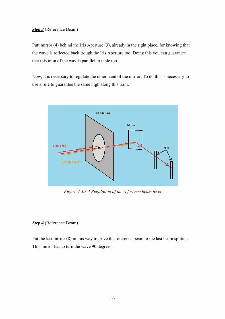
Step 3 (Reference Beam)
Putt mirror (4) behind the Iris Aperture (3), already in the right place, for knowing that
the wave is reflected back trough the Iris Aperture too. Doing this you can guarantee
that this tram of the way is parallel to table too.
Now, it is necessary to regulate the other hand of the mirror. To do this is necessary to
use a rule to guarantee the same high along this tram.
Figure 4.3.3.3 Regulation of the reference beam level
Step 4 (Reference Beam)
Put the last mirror (8) in this way to drive the reference beam to the last beam splitter.
This mirror has to turn the wave 90 degrees.
66
Step 5 (Reference Beam)
Calibrate optical lends used in the reference beam to assembly a telecopy system.
The first lend that is going to be collocated is a Defocusing Lend or Concave Lend. This
lend rises the speck of the laser proportionally with the distance respected this lend.
To put the speck in the middle of the lend it is necessary to put a paper behind the lend
and see if the speck is in the middle of the lend.
This is so roughly, so later on it will be accurate approximated with the mirrors.
Once it is done, it is collocated the Concave Lend.
To put the second lend in the right place, it is necessary to know which kind of
telescopic system we are assembling. So, there are two possibilities.
First possibility
With a Focusing Lend or Positive Focusing Lend and a Convex Lend.
In this system the focus of the Focusing Lend is behind it, so if the big Convex Lend is
for X mm, it has to be collocated X mm from the focus.
Figure 4.3.3.4 Positive telescopic system
67
Second possibility
With a Defocusing Lend or Negative Focusing Lend and a Convex Lend.
In this system the focus is in front of the Defocusing Lend, so the Convex Lend will be
collocated X mm from this focus.
This distance will be lower than in the first possibility.
Figure 4.3.3.5 Negative telescopic system
In my case, I am using a Defocusing Lend (6) of 25 mm and a Convex Lend (7) of 500
mm. So, the Convex Lend (7) has to be 475 mm from the centre of the Defocusing Lend
(6).
The way to regulate and collocated in the right place both lends is the next.
First of all is necessary to centre the speck of the laser in the centre of the Defocusing
Lend (6). To do this it possible to use a dark paper and put it behind the lend and see
that the speck is roughly in the middle of it.
68
Figure 4.3.3.6 Regulation of the Defocusing Lend
Now, it is necessary guarantee that the expanded speck fits into the Convex Lend (7).
This is also made through a dark paper (like brown paper) putting it in front of the lend
and regulating the big speck like is shown in the next figures:
Figure 4.3.3.7 Regulation of the horizontally of the convex lend
69
Figure 4.3.3.8 Regulation of the vertically of the convex lend
Step 6 (Illumination Beam 1)
Put again an Iris Aperture (9) behind the Beam Splitter (2). Then I put a mirror (16) to
know where has to be directed the beam. But now, I only use this mirror to guarantee
that the beam is come back to the Iris Aperture (9) in a right way.
Once I have done this, I must turn the mirror (16) and point with the metal beam. To do
this correctly, it is necessary use a rule to guarantee the same high along the last tram of
the way.
The procedure is identically to the step 3.
70
Step 7 (Illumination Beam 2)
Put a mirror (10) behind the Iris Aperture (9) to deviate the beam 90 degrees. Then I
have to drive the way equal that in the step 6. Finally, the two specks of the two
Illumination Beams have to be in the same place in the metal beam (18).
Step 8 (Illumination Beam 1 and 2)
Put the different lends in this two ways (Concave Lend 12 and 15).
In this case, I am going to use only a Defocusing Lend with out Convex Lend; for this
reason I only have to be into account putting the Defocusing Lend respect the mirror in
an enough length to allow that the expanded speck fits in the mirror.
The procedure is similar to the step 5, without the Convex Lend.
Step 9 (three both beams)
Now I have assembled the three ways; it is necessary to put the last Beam Splitter (19)
in a right place.
To do it, I need to put a mirror instead putting the metal beam (18). This does that the
mirror reflects the Illumination Wave perfectly into the Beam Splitter (19), then the
Beam Splitter superpose the two beams and you can see if they are accurate superposed.
To do this correctly, it is necessary putting an Iris Aperture (17 and 14 for Illumination
Beam 1 and 2 respectively) before the beam arrives to the metal beam. So in this way,
you can approximate the size of the speck of Illumination Wave to the size of the speck
of Reference Wave.
This comparison can be carried on with a piece of paper. For example, if you first block
one wave you only see the speck of one wave, so you could mark in the paper with a
pen where exactly this speck is. Later, you can block the other beam and do the same
with the other.
So, you can compare the two big specks and know exactly where putting the Beam
Splitter (19).
71
And finally, the CCD-Camera (20) is placed really closed to the Beam Splitter (19). The
only thing that has to be realize carefully is guarantee that sensor of the CCD is in the
middle of the laser speck.
Figure 4.3.3.9 Regulation of the last beam splitter for the illumination beam
Figure 4.3.3.10 Regulation of the last beam splitter for the reference beam
72
It is important to highlight the utilization of rails in the ways of the two illumination
ways. It is important because of the path length. So first of all, the way of the Reference
Beam has been assembly and after the other two ways. These have been assembly with
a path length roughly equal than the path length of the Reference Beam, and after have
been accurate these two distances through the graph rail.
So, the real assembly in the lab is like is shown in the next two figures:
Figure 4.3.3.11 Real assembly in the holography lab 1.
Figure 4.3.3.12 Real assembly in the holography lab 2.
73
4.4- Problems Encountered
One of the main problems was the huge difference brightness between the Reference
Beam and the two Illuminations Beams.
So, knowing this problem, it was looked for some possible sources of the problem,
which were:
Polarization in different direction: To solve this situation it was placed a Polarization
Rotator in front of the first Beam Splitter (2); so managing this device it was observed
that the brightness of the three beams were changing.
And finally, the Reference Beam and the Illumination Beam were polarized at 90
degrees, so it was impossible to achieve any kind of interferometry.
To correct this problem I turned the casing of the laser till the polarizing was different
of 90 degrees and the brightness of the Reference Beam and Illumination Beam were
similar.
Nevertheless, another problem related with the brightness arose. It was that the light
reflected in the metal beam was extremely low, so it was necessary putting a filter (5) in
the way of the Reference Beam to reduce its brightness and approximate it to the
brightness of the Reflected Beam.
To measure and regulate it in an exactly way, I used Laser Power Meter that told me
what was the exactly power (in mW) of each wave.
Once solve this little problem it was time to record some hologram, but it resulted
impossible.
First source of the problem that was though was the path length of the different beams
were wrong and the difference was upper than a few centimeters. So to check it, the
laser was changed by an Nd-YAG Laser which coherence length is around 30 metres (I
had to change the filters because this laser was much more powerful (around 100 mw)
and it was impossible to watch nothing in the screen of the computer.)
The result was unsatisfactory because it was impossible to watch some kind of
interference of the beams on the screen of the laptop.
74
4.5- Results Obtained
Once resolved the problem of the polarization and the brightness seemed that it was
going to be possible to take a hologram.
It was unsatisfactory and the results were the same.
To check if it was everything perfect, the metal beam was changed by a mirror that
reflected the Illumination Beam into Beam Splitter (19).
Now, the results were different. In the hologram there were the typical fringes but not
well defined and some tiny diagonal fringes.
These tiny diagonal fringes show that there is some kind of interferometry, so it means
that the two waves are arriving almost well.
However, the other fringes which were due to Reference Beam were really big and
really dirty.
So, it seems that the beams arrive with a lot of noise.
Another aspect that it is important to result is that when you knocked very weakly the
table of the lab the diagonal fringes disappeared what show that if something perturbs
the environment of the lab the interferometry between the two beams is over.
4.6- Applicable Improvements
Now, knowing the problems for taking a hologram, there is something that can be done
to improve it.
One of these things is clean perfectly each component and check very quietly that all of
them are right.
And the second thing that will be good to do it is changing whole components one by
one and realized which one is the focus of the problem.
75
5- Discussion and Interpretation
If it is compared the obtained results of the point B by Finite Element Analysis and by
Dänliker Algorithms is easy to guess that these results are bit different.
These results can be observed in the appendices I and II respectively. In the appendix I
the point with its strains and stresses is shady by orange color.
The reason because both results are a bit different is due to the size of the mesh (1 mm)
is so huge; the program (Abaqus) could not process a smaller mesh.
Like Finite Difference is an approximation of the derivate’s meaning and it is a limit
going to infinite; it is usual that an increment of 1 mm was so long.
Another important reason is the approximation of the turned angle by the metal beam to
zero [10]. It can variety a little the final result, but it does not have as importance as the
last justification.
Nevertheless it is important to remark that the stresses obtained by FEM and Dänliker
algorithms are really different because the strains are bit different, and this makes that
the difference for the stress will be huger than the difference for the strain.
And finally it is important to say, that if you compare a result of Finite Element Method
with one of Finite Difference both of them are approximations of the result; so is
common that they were not the same.
Other aspects about Dänliker algorithms have been discussed at the end of that chapter.
The result of the holography set up have been explained in the chapter four previously.
76
6- Conclusions
The global result of the project is successful.
The reason of this is because a lot of different aspects like FEM, Dänliker algorithms
and Digital Holography have been mixed to obtain some result and compare them. With
this comparison we can know if the Dänliker algorithms mixed with Digital Holography
are enough good for trusting them.
Nevertheless, this project is a brief study of something that can have a big impact in the
industry because it is one way for obtaining the behavior inside an object without
damaging it.
However, the objective of this project is not to analyze the different results if not only
compare them. It means, comparing the results coming from Finite Element Method and
the results coming from Digital Holography and Dänliker algorithms; and see that they
are more or less the same.
So, of my point of view, this is a field that it is necessary to study deeper because it is a
way to achieve good tests for some jobs that need a high level of security like can be
aircraft industry or something similar to it.
77
7- Recommendations and Suggestions for Future Work
For future work is important taking into account approximate deeper the Dänliker
algorithms with increments as short as possible.
Nevertheless, it will be important to get a mesh in FEM much thinner, like 0,1 mm. The
result of this will be more exactly and then the comparison between FEM and Dänliker
will be better.
With respect to the holography set up, the task will be to check component by
component and know which one is wrong and finally clean all of them.
Later on, the mission will be recording a hologram and if it is successful, measuring the
displacement of the metal beam with special software.
This part can be the hardest, because it can take an interval of time undefined. So, it is
important doing this improvement step by step and always noting down all different
aspects.
78
8- References
Books:
1. W. Jueptner, U. Schnars, 2005, “Digital Holography”, Springer
2. Edgar Conley, Jean Robillard, 2000, “Industrial Applications for Optical Data
Processing and Holography”, CRC Press
3. D. J. Wave, 1984, “Matrix and finite element displacement analysis of
structures”, Oxford University Press
4. B. J. Bell, M. J. Smith, 1980, “Theory of Structures”, George Godwin
Before using a laser is necessary to know a little about laser safety and how to use in a right way the lasers and all the things that are involving this field.
The word laser is an acronym for Light Amplification by the Stimulated emission of Radiation. The ‘light’ produced by a laser, a form of non-ionising optical radiation, has a unique combination of spatial coherence (all the waves are in phase); monochromaticity (i.e. have just one colour or a narrow bandwidth) and usually high collimation (i.e. low angular divergence such that the beam does not ‘spread out’ significantly with distance). This combination of characteristics distinguishes laser radiation from all other light sources. Lasers come in various shapes and forms. They have many uses in teaching, research, manufacturing, medicine, dentistry, shop checkouts and most commonly at work in the office. Lasers emit radiation as narrow concentrated beams of light, not necessarily visible to the human eye. The optical and skin hazards presented by lasers vary markedly according to the wavelength an power of the output. The hazards of lasers are often associated with the ability of the laser to damage eyesight or burn skin, but quite often the radiation or optical hazards are not the ones that present the greatest risk, with associated risks from electrical supplies, cryogenic liquids or chemical dyes being more hazardous. There is a legal requirement to identify risks and take appropriate action to eliminate or control those risks. We all have a responsibility under the Health & Safety at Work etc. Act 1974 to ensure that work with lasers is carried out safely. Users have a duty to protect both themselves and others from the potential hazards involved, particularly when working with the more powerful lasers. The safety of laser products is covered by the British Standards Institute (BSi), BS EN 60825 series of documents. The BS standard is a ‘euronorm’ based upon the corresponding International Electrotechnical Commission’s IEC 60825 standard encompasses a range of standards for manufacturers on lasers, fibre optic systems, laser guards, components and user’s guide etc. Of particular importance for users is the Technical Report PD IEC TR 60825-14:2004 which is a new detailed user’s guide that incorporates a risk assessment approach to laser safety. Many Institutions have internet access to British Standards Online and have licence subscriptions allowing standards to be downloaded. Each institution should at least have access to Technical Report PD IEC TR 60825-14:2004 or its current version.
120
The previous classification system, which was based on five classes (1, 2, 3A, 3B and 4), has been replaced with a new system of seven classes (1, 1M, 2, 2M, 3R, 3B and 4). It should be noted however that most of the changes relate to the lower classes of laser and that there has been minimal changes to the requirements for Class 3B and Class 4 lasers.
First of all, the laser users have some responsibilities which are the next:
• To observe the Local Rules and Schemes of Work applicable to the lasers that will be used and to follow the guidance of supervisors and the Departmental Laser Safety Officer.
• Not to leave a laser experiment running unattended unless a risk assessment has established that it is safe to do so.
• For their own safety and that of others who may be affected by their acts or omissions.
• When working with Class 3B or Class 4 lasers and there is the possibility of stray laser beams that could damage the eyesight, the appropriate laser eyewear must be worn.
It is also necessary to know the different classes of lasers ant their hazards, and how works a laser before using it. Lasers produce electromagnetic radiation at wavelengths extending from 100 nm in the ultraviolet, through the visible (400-700 nm), and the near infrared (700-1400 nm), to the far infrared (1400 nm – 1 mm). Thus, the light emitted can be either visible or invisible. Lasers can be operated in a number of different modes. Some lasers produce a continuous output and are known as continuous wave or CW lasers. The power outputs of CW lasers are usually expressed in terms of watts (W). Others operate in a pulsed mode producing short bursts of radiation. The power of the laser output can vary from less than 1 mW to many watts in some CW devices. The energy output of pulsed lasers is generally expressed in joules (J) per pulse. Because of the wide ranges possible for the wavelength, energy content and pulse characteristics of laser beams, the hazards arising from their use varies widely. It is impossible to regard lasers as single group to which common safety limits can apply. A system of laser classification is used to indicate the level of laser beam hazard and maximum Accessible Emission Levels (AELs) have been determined for each class of laser. The previous classification system, which was based on five classes (1, 2, 3A, 3B and 4), has been replaced with a new system of seven classes (1, 1M, 2, 2M, 3R, 3B and 4) and these are described below [7].
121
• Class 1: Lasers that are safe under reasonably foreseeable conditions of operation, either because of the inherently low emission of the laser itself, or because of its engineering design such that it is totally enclosed and human access to higher levels is not possible under normal operation. If access panels of a totally enclosed system are removed for servicing etc then the laser product is no longer Class 1 and the precautions applicable to the embedded laser must be applied until the panels are replaced.
• Class 1M: Lasers products emitting in the wavelength range 302.5 nm to 4000 nm, whose total output is in excess of that normally permitted for Class 1 laser products but because of their diverging beams or very low power density do not pose a hazard in normal use and comply with the measurement conditions for a Class 1M product. However they may be hazardous to the eyes under certain conditions if gathering optics are used with them, i.e.
a) With a diverging beam if optics are placed within 100 nm of the source to concentrate/collimate the beam.
b) With a large diameter collimated beam viewed with binoculars or a telescope.
• Class 2: Lasers that only emit visible radiation in the wavelength range from 400 nm to 700 nm and whose output is less than the appropriate AEL. They are safe for accidental viewing as eye protection is afforded by aversion responses, including the blink reflex. This reaction may be expected to provide adequate protection under reasonably foreseeable conditions of operation including the use of optical instruments for intrabeam viewing.
• Class 2M: Laser products that only emit visible radiation in the wavelength range 400 nm to 700 nm, whose total output is in excess of that normally permitted for Class 2 laser products but because of their diverging beams or very low power density are safe for accidental viewing during normal use and comply with the measurement conditions for a Class 2M product. However they may be hazardous to the eyes under certain conditions if gathering optics are used with them, i.e.
a) With a diverging beam if optics are placed within 100 nm of the source to concentrate/collimate the beam.
b) With a large diameter collimated beam viewed with binoculars or a telescope.
• Class 3R: Lasers that emit in the wavelength range from 302.5 nm to 1 mm where direct intrabeam viewing is potentially hazardous but the risk is lower than for Class 3B lasers, and fewer manufacturing requirements and control measures for the user apply. The AEL is restricted to no more than five times the AEL of Class 2 for visible wavelengths and no more than five times the AEL of Class 1 for other wavelengths.
• Class 3B: Lasers that are normally hazardous when direct intrabeam exposure occurs (i.e. within the Nominal Ocular Hazard Distance, which is the distance
122
within which the beam irradiance or radiant exposure will exceed the appropriate MPE). Viewing diffuse reflections is normally safe. Output levels must be less than the appropriate AELs for Class 3B devices.
• Class 4: High power lasers that exceed the AELs for Class 3B products that are also capable of producing hazardous diffuse reflections. They may cause skin injuries, could also constitute a fire hazard and could cause hazardous fumes to be produced as well as being a hazard to the eyes. Their use requires extreme caution.
In this way, it is visible in the next table the different hazards, precaution, controls and Limits in each kind of laser class.
Laser Class
Hazard Precaution Controls Limits & Comments
1 Intrinsically safe under reasonably foreseeable conditions or by good engineering design.
Do not stare into beam. Protection by blink reflex.
No access allowed. Very low exposure
250 μJ in 0.25s 1 mW cw
1M Wavelength 302.5 – 4000 nm. Intrinsically safe under reasonably foreseeable conditions or by good engineering design. Potentially hazardous when viewed by an optical instrument.
Do not stare into beam. Protection by blink reflex BUT do not view with optical instruments.
No access allowed. Very low exposure
250 μJ in 0.25s 1 mW cw
2 Low power cw or pulsed lasers in visible region (400 nm - 700 nm)
Do not stare into beam. Protection by blink reflex.
Momentary exposure not hazardous
1 mW cw 1 mW peak power.
2M Low power cw or pulsed lasers in visible region (400 nm - 700 nm). Potentially hazardous when viewed by an optical instrument.
Do not stare into beam. Protection by blink reflex BUT do not view with optical instruments.
Momentary exposure not hazardous
1 mW cw 1 mW peak power.
3R Lasers in range 302.5 – 106
nm where direct intrabeam viewing is hazardous. Viewing with optical aids may be hazardous.
Do not stare into beam or view directly with optical instruments.
Momentary exposure not hazardous if optical aids not used
5 mW cw 6 J/m
2 in 0.25 s
25 W/m2 in
0.25 s
123
3B Lasers in range 302.5 – 106
nm where direct intrabeam viewing is hazardous. Direct viewing hazardous. Diffuse reflections normally safe.
Avoid exposure to beam. Direct intra-beam viewing is hazardous.
Controlled area. Eye protection if direct/specular viewing possible.
30 mJ for ruby 0.5 W cw for HeNe, argon etc
4 High power devices above 0.5 W. Diffuse reflections hazardous. Skin injuries possible. Fire hazard
Avoid eye or skin exposure to direct or scattered radiation.
Controlled area. Extreme caution required. Enclosed beams. Remote control if possible.
CO2, ruby, YAG, argon, excimer...
Table 9.3.1 Classification of the lasers
Once classified the different classes of laser, it is necessary to speak a little about labeling of lasers, designation of laser areas and laboratory design.
Labelling of Lasers
Inherently safe lasers in Class 1 do not need warning labels but lasers which are Class 1 by engineering design and contain an embedded laser of higher power should be labeled as ‘Class 1’. Supplementary information describing the laser product as a ‘Totally Enclosed System’ with details of the embedded laser clearly displayed may be of value in situation where access to the embedded product is routinely required. All other laser products should carry the appropriate warning labels in accordance with BS EN 60825-1. Recently manufactured lasers should all conform to this Standard. Where lasers and laser systems are not adequately labeled (some American systems have very small labels that are hard to read and do not comply with our BS), they will need to be relabeled. Institutions should note that for mains powered equipment the labeling of lasers in future will have to comply with European Standards and any institution obtaining a laser directly from the US will assume the responsibilities of the importer and supplier.
124
Designation of Laser Areas The points of access to areas in which Class 3B and Class 4 lasers are used must be marked with appropriate warning signs. There may also be experiments where open beam work with modified Class 1M/Class 2M or Class 3R lasers are used that will also warrant the display of appropriate warning signs. Laboratory Design The following considerations relate mainly to the use of Class 4 lasers but some may be appropriate for Class 3B devices as well, or, as general specifications for a laser laboratory. If practicable the laser laboratory should have a high level of illumination that will reduce the risk of stray laser light reaching the retina. Windows should be kept to a minimum and may need to be covered or protected by blinds. These should be non-reflective and may need to be fireproof where higher-powered lasers are used. Walls, ceilings and fittings should be painted with a light coloured matt paint to enhance illumination and minimize specular reflections. Reflecting surfaces such as the use of glass-fronted cupboards should be avoided. Ventilation is important especially with higher-powered lasers if cryogens are used, or if toxic fumes are produced that need to be extracted and in this case it is important that the extraction is very close to the source. Facilities may also be needed for the handling of toxic chemicals that are associated with some dye lasers. The laboratory should be equipped with appropriated firefighting equipment. Electrical supplies, switch and control gear should be sited in order to:
• Enable the laser to be shut down by a person standing next to the laser. • Enable the laser to be made safe in an emergency from outside the laser area if
reasonably practicable. • Prevent accidental firing of a laser. • Provide an indication of the state of readiness of the laser. • Enable personnel to stand in a safe place. • Provide sufficient and adequate power supplies for all ancillary equipment and
apparatus so that the use of trailing leads is minimized. Once, it is explained in a little way about the lasers and their hazards, it will be good write the general rules that have to be follow in the lab.
125
• Never stare into a laser beam, unexpanded or not. • Never look at specular reflections of a laser beam.
If present try to minimize or eliminate If this is not possible understand the reflective nature of material
• Wear laser safety goggles at all times. Choose the appropriate eyewear for wavelengths you are working at. Choose the appropriate density for total or partial block.
• Never point a laser at anyone • Never move a laser while it is switched on.
Never move any associated equipment such as power supplies or gas bottles when laser is on.
• Never allow visitors into the lab without your permission. Rectrict number of visitors Ensure that visitors are properly briefed into the hazards. Ensure the visitors are sufficiently protected (eyes and skin).
• When entering a laser lab always knock loudly and wait for a signal to enter If no signal is given enter cautiously.
• Do not touch electrical supplies. • Keep walkways clear at all times.
In case of an emergency involving the laser, electrical equipment, personnel, fire, etc:
Lasers
• Switch off the unit immediately by hitting the RED stop button located on the
laser power supply and the laser head • Where possible isolate the laser from the supply by disengaging the main
isolator • If appropriate, sound the FIRE alarm • In case of injury due to exposure to laser radiation (particularly to the eye) or
suspected exposure, the injured person should be taken to A&E at ARI, Foresterhill and treated appropriately. Details of the laser should be taken along to help the diagnosis and treatment.
126
Electrical equipment
• Isolate the equipment from the electrical supply immediately; beware of wet areas in the vicinity
• Do not touch injured party until the isolation is complete. YOU run the risk of injury if you fail to do so
• If appropriate sound the FIRE alarm • In case of injury, the injured person should be taken to A&E at ARI,
Foresterhill and treated appropriately.
And finally, a list of several important rules for lasers and optical systems.
• Ensure that anyone present in the room is wearing protective eyewear. • Operate the laser on its lowest possible setting (as indicated on the laser power
supply). • Remove watches and reflective jewellery before any alignment activities begin. • Check on the stability and rigidity of all optical mounts, beam blocks and stray
beam shields. • Ensure that the unexpanded beam cannot be directly accessed by the eye or with
optical aids. • Make sure the beam can never rise to eye level. • Do not bend down to eye level. • When placing mirrors into the beam, always start with mirrors facing
downwards. • Never move a mirror unless you know where the beam will go. • Do not direct laser beams outside the confines of the table. • Do not direct stray laser beams outside the confines of the table. • Enclose all beam paths as far as possible. • Ensure that stray laser light cannot leave the room. • The arrangement should be inspected by lab supervisor before the laser is turned
up to full power. • Post a warning sign outside alerting visitors and colleagues to your activities. • When using high power gas lasers (e.g. argon or CO2).
Never place highly reflective material such as copper or aluminium in the beam path unless you are sure of the requirements needed to process/study/use the material.
Never place material that will cause damage to the lens system e.g. wood, perspex, and brittle materials into the beam path.
• Never open lasers, controllers or transformers without supervision since most lasers use high voltage supplies.
127
• Be aware of presence of high pressure tubes, toxic chemicals, gases, etc.
• Never attempt to operate a water or air-cooled laser with cooling turned off. When powering down a water-cooled or air-cooled laser the coolant is