measurement systems laboratory massachusetts institute of technology. cambridge massachusetts 02139 TE.- 49 APPLICATION OF CONTRACTION MAPPINGS TO THE CONTROL OF NONLINEAR SYSTEMS BY William Robert Killingsworth, Jr. CASE: FILE CORY,
Transcript
measurement systems laboratorymassachusetts institute of technology. cambridge massachusetts 02139
TE.- 49
APPLICATION OF CONTRACTION MAPPINGS TOTHE CONTROL OF NONLINEAR SYSTEMS
BY
William Robert Killingsworth, Jr.
CASE: FILECORY,
TE -49
APPLICATION OF CONTRACTION MAPPINGS TO
THE CONTROL OF NONLINEAR SYSTEMS
by
William Robert Killingsworth, Jr.
January, 1972
Measurement Systems Laboratory
Massachusetts Institute of Technology
Cambridge, Massachusetts 02139
APPROVED: M ac)DirectorMeasurement Systems Laboratory
APPLICATION OF CONTRACTION MAPPINGS TO
THE CONTROL OF NONLINEAR SYSTEMS
by
WILLIAM ROBERT KILLINGSWORTH, JR.
B.S., Auburn University, 1966
M.S., Massachusetts Institute of Technology, 1968
SUBMITTED IN PARTIAL FULFILLMENT
OF THE REQUIREMENTS FOR THE
DEGREE OF DOCTOR OF PHILOSOPHY
at the
MASSACHUSETTS INSTITUTE OF TECHNOLOGY
January 1972
Signature of Author /Cln Department of Aeronauticsjand Ast onautics
Chairman, Departmental Co ittee o Graduate Students
APPLICATION OF CONTRACTION MAPPINGS TO
THE CONTROL OF NONLINEAR SYSTEMS
by
William Robert Killingsworth, Jr.
Submitted to the Department of Aeronautics and Astronautics on January 14,1972 in partial fulfillment of the requirements for the degree of Doctor ofPhilosophy.
ABSTRACT
This research considers the theoretical and applied aspects of successiveapproximation techniques for the determination of controls for nonlinear dynamicalsystems. Particular emphasis is placed upon the methods of contraction mappingsand modified contraction mappings. It is shown that application of the Pontryaginprinciple to the optimal nonlinear regulator problem results in necessary con-ditions for optimality in the form of a two point boundary value problem (TPBVP).
The TPBVP is represented by an operator equation and functional analytic results
on the iterative solution of operator equations are applied. The general con-vergence theorems are translated and applied to those operators arising from
the optimal regulation of nonlinear systems. It is shown that simply structuredmatrices and similarity transformations may be used to facilitate the calculation
of the matrix Green's functions and the evaluation of the convergence criteria.A controllability theory based on the integral representation of TPBVP's, the
implicit function theorem, and contraction mappings is developed for nonlineardynamical systems. Contraction mappings is theoretically and practically appliedto a nonlinear control problem with bounded input control, and the Lipschitznorm is used to prove convergence for the nondifferentiable operator. A dynamicmodel representing community drug usage is developed and the contraction mappingsmethod is used to study the optimal regulation of the nonlinear system.
Thesis Supervisors:
Professor John J. Deyst, Jr.
Title: Associate Professor of Aeronautics andAstronautics, MIT
Professor Peter L. Falb
Title: Professor, Division of AppliedMathematics, Brown University
Professor Edward B. Roberts
Title: Professor of Management, MIT
Page intentionally left blank
ACKNOWLEDGEMENTS
The author wishes to thank his thesis committee: Professor John J. Deyst,
committee chairman, whose guidance and encouragement were invaluable; Professor
Peter L. Falb who generously provided many hours of fruitful discussions and whose
work provided the basis and motivation for the thesis; and Professor Edward B.
Roberts whose incisive comments and thought provoking discussions were highly
valued The unique perspective and penetrating insight of each of these gentlemen
has made association with this committee a particularly rewarding experience for
the author.
Special thanks are due to Professor Walter Wrigley who provided guidance and
encouragement throughout the author's doctoral program.
The author is indebted to Dr. Robert Stern and the staff of the Measurement
Systems Laboratory who gave freely of their time and energy.
Thanks are also due to Miss Marjorie Goldstein whose conscientious efforts
in typing the thesis are gratefully acknowledged, and to Mrs. Ann Preston for
preparation of the figures and attending to the many details of publication.
Finally, the author wishes to extend special thanks to his dear wife Joyce
for her unfailing support, encouragement, and patience throughout this endeavor.
This research was supported by a grant from the National Aeronautics and
Space Administration, NGR 22-009-010 and NsG 22-009-270.
The publication of this thesis does not constitute approval by the National
Aeronautics and Space Administration or by the MIT Measurement Systems Laboratory
of the findings or the conclusions contained therein. It is published only for
the exchange and stimulation of ideas.
Page intentionally left blank
'TABLE OF CONTENTS
Chapter Page
1 INTRODUCTION 1
1.1 Background 1
1.2 Description of the Problem 3
1.3 Synopsis 4
2 OPTIMAL REGULATION OF NONLINEAR SYSTEMS 7
2.1 Introduction 7
2.2 Optimal Linear Regulator 7
2.3 Optimal Regulation of Nonlinear Systems 11
3 METHODS OF SOLVING TPBVP's 19
3.1 Introduction 19
3.2 Representation of TPBVP's 19
3.3 Frechet Derivatives and Lipschitz Norms 23
3.4 Contraction Mappings Method 26
3.5 Modified Contraction Mappings 31
3.6 Applications of Contraction Mappings 36
4 CALCULATION OF CONVERGENCE CRITERIA 43
4.1 Introduction 43
4.2 Evaluation of Convergence Criteria 44
4.3 Boundary Value Sets of Interest 46
4.4 Boundary Set for Regulation wiht Terminal Cost 47
vii
Page
4.5 Boundary Set for Regulation with No Terminal Cost 54
4.6 Application of Similarity Transformation 56
4.7 Approximate Technique 66
5 CONTROLLABILITY FOR NONLINEAR SYSTEMS 71
5.1 Introduction 71
5.2 Controllability for Linear Systems 71
5.3 Nonlinear Controllability 75
5.4 Evaluation of Controllability Convergence Parameters 84
6 NUMERICAL EXAMPLES 91
6.1 Introduction 91
6.2 Van der Pol's Equation 92
6.3 Null Controllability with Bounded Control 102
6.4 Controllability of Satellite Pitch Motion 109
7 PRELIMINARY STUDY ON THE DYNAMICS OF DRUG USAGE WITHIN A COMMUNITY 119
7.1 Introduction 119
7.2 Development of a Dynamic Model 120
7.3 Optimal Regulation of the Nonlinear System 130
8 SUMMARY, CONTRIBUTIONS AND RECOMMENDATIONS 141
8.1 Summary 141
8.2 Contributions 143
8.3 Recommendations 143
Appendix 145
' A Description of Contraction Mappings Computer Algorithm 145
Bibliography 173
viii
LIST OF FIGURES
Figure
6.1 The sphere
6.2 The sphere
Page
96
98
6.3 Control iterations 101
6.4 Comparison of performance for contraction mappings and modified 102
contraction mappings
6.5 The sphere g(yo,r)
6.6 The sphere (ycl,r) for T =
6.7 The sphere g(yo,r) for T = Tr/2
6.8 State and control history
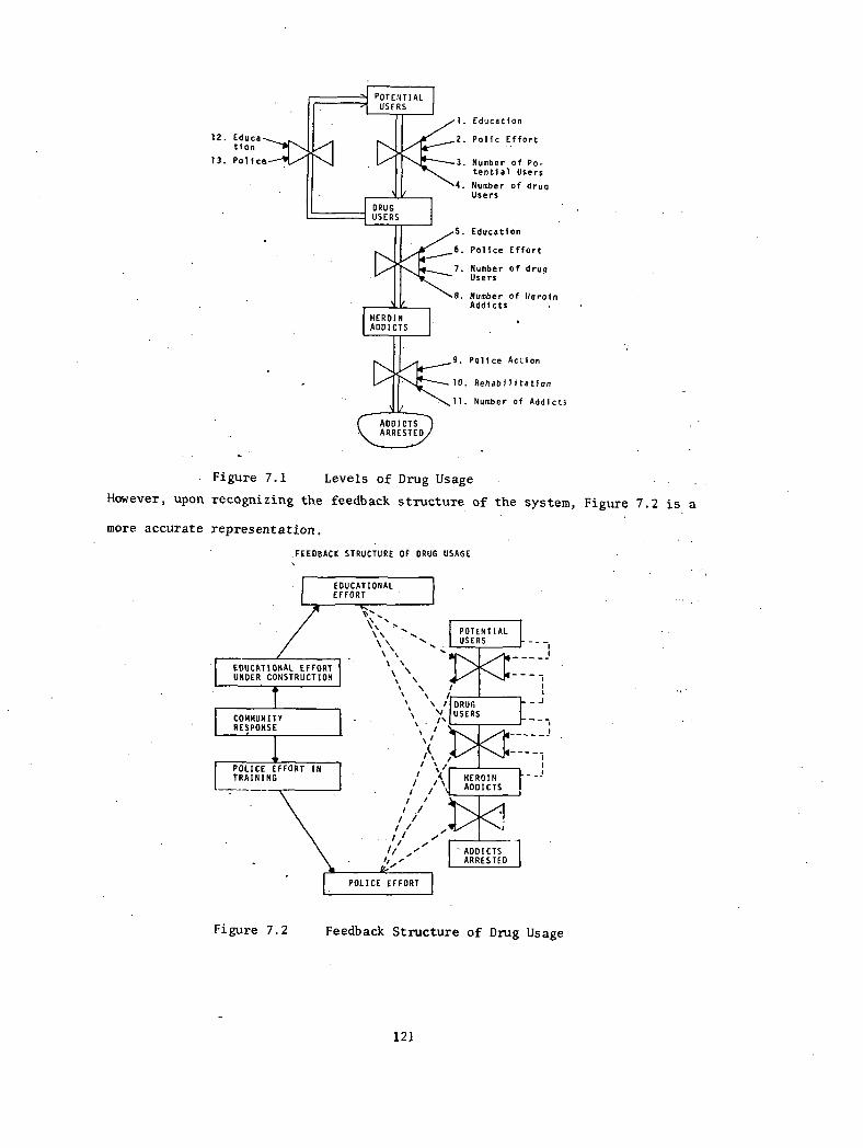
7.1 Levels of drug usage
7.2 Feedback structure of drug usage
7.3 Availability of Potential Users multiplier
7.4 Availability of Drug Users multiplier
7.5 Effect of education on addiction growth rate
7.6 Police effectiveness
7.7 Availability of Addicts multiplier
7.8 Police effectiveness
7.9 Effect of education on addiction growth rate
7.10 The function y0(t) for T = 12 months
7.11 Addicts, Police, and Education for T = 12 months
7.12 The function y0(t) for T = 48 months
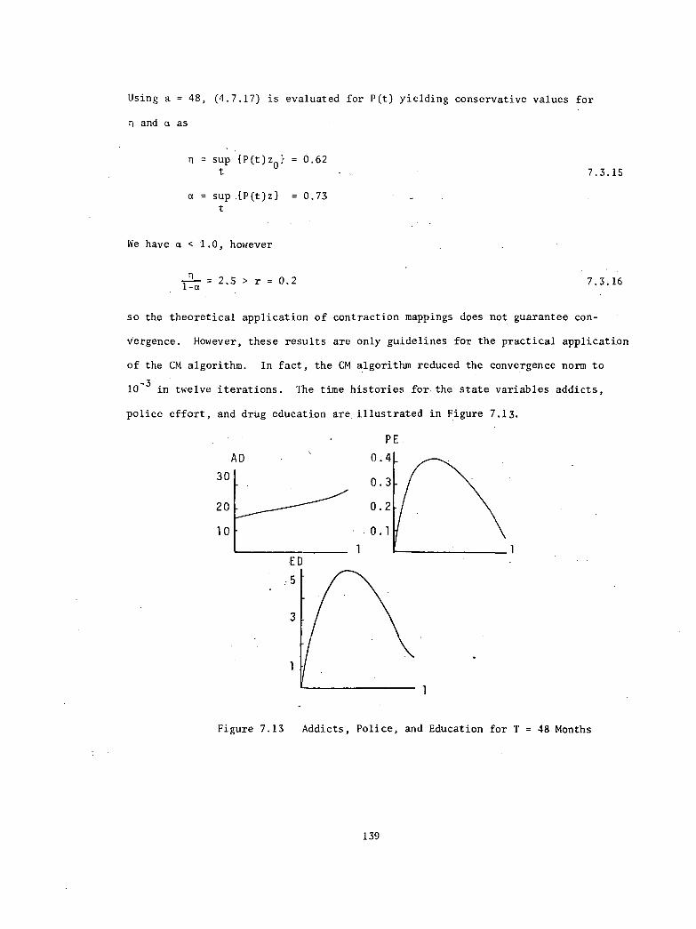
7.13 Addicts, Police, and Education for T = 48 months
ix
106
112
115
117
121
121
124
125
126
127
128
134
134
135
137
138
139
CHAPTER t
INTRODUCTION
1.1. Background
Optimal control theory has experienced an increasing growth of interest in
the past two decades. Initially motivated by the aerospace effort, optimal control
theory is now involved in many aspects of general systems engineering. Applica-
tions range from chemical process control to attempts at managerial and economic
planning.
One of the most important and most widely treated problems to date in
optimal control theory is the so-called "Linear Regulator Problem". Historically,
this problem arose in Wiener's work concerning stationary time series and linear
filtering and prediction [W1]. Under the name 'Minimum Integral Squared Error",
development of this problem was continued through the 1950's by Newton [N1],
Booten [B3],and Zadeh [Z1]. Finally utilizing the techniques of modern control
theory, Kalman [K1] presented important new aspects of the problem.
The prominence of this problem is' due to two primary factors. First, the
problem provides a strong link between the classical methods of analytic feedback
system design via frequency domain methods and the more recent variational approach
favoring analysis in the time domain [K4], [W2]. Secondly, the problem allows the
determination of optimal controls in closed form with mathematical ease. (For
general development and presentation of the problem, see Athans and Falb' [A1] and
Lee and Markus [L1]). Finally, a pragmatic motivation for considering the
problem is the ease with which the quadratic cost criteria can be interpreted
1
z
physically. Consequently, optimal linear regulation has been extensively
applied to various systems. For example, the theory has found widespread
applications in the area of automatic flight control systems. Much of this
work is based on the significant efforts of Rynaski [R4], [R5]. Other examples
of optimal linear regulation are contained in Dyer and McReynolds [D2].
However, few systems can adequately be described by a linear dynamic model.
In particular, increasing effort is now being devoted to the development of
models representing systems as varied and as complex as urban areas, natural
resource depletion, management of R and D efforts, and drug usage within a
community. These models are primarily due to the efforts of Forrester [F3,
F4,F5,F6] and Roberts [R2]. Along with many engineering systems, these systems
contain inherent nonlinearities which must be included in any meaningful study.
In contrast to linear systems, the regulation of nonlinear dynamical systems
has received limited attention, most of a specialized nature. The primary reason
for this seems to lie in the fact that nonlinear optimal control problems can
rarely be solved analytically or, more specifically, in feedback form as for
linear regulators. As a result, one must often resort to iterative numerical
techniques for the determination of the optimizing solutions. Consequently, much
of the analysis regarding regulation of nonlinear systems concerns techniques for
determining suboptimal feedback controllers. (See for example [D1], [G2], [L3],
[P1], [S2], [J1], [F8], and [B5]). Most of these approaches involve the modeling
of the nonlinear system as a linear system in some manner. A somewhat different
approach, not suboptimal, is taken by Brunovsky [B4] and Lukes [L4]. Both of
these treatments are closely related to the basic hypothesis that the system be
stabilizable [L1]. Under the assumption of complete controllability, Brunovsky
approached the problem via Lyapunov functions. Lukes requires the system be
2
stabilizable and then uses Lyapunov-like theory to obtain results for feedback
controllers.
The direction of these various approaches is primarily generated by the
desire for a feedback controller. However, there is a second, more esoteric
reason, and that is the desire for general results. Unfortunately, the undis-
cerning application of an algorithm often limits insight into the underlying
structure of the problem being considered. This loss of general information is
often due to the fact that practical convergence criteria are few for most of
the iterative methods used in the solution of optimal control problems. Theoreti-
cal aspects of these criteria have been investigated by numerous applied mathe-
maticians (see Kantorovich [K4] and Collatz [C2]). The Russian Kantorovich [K4]
was one of the first to develop and unify the mathematical theory of iterative
methods. Using the power of functional analysis methods, he presented conver-
gence results for such basic iterative schemes as contraction mappings and
Newton's method. These basic results have been considerably broadened, modernized,
and made practical by the efforts of Falb and de Jong [F1]. In their book, they
present the derivation of general convergence criteria for the application of
various successive approximation methods to the solution of optimal control
problems.
1.2. Description of tha Problem
The primary goal of this research is the consideration of the theoretical
and applied aspects of successive approximation techniques for the solution of
optimal nonlinear regulator problems. Application of the Pontryagin principle
to the posed optimization problem results in necessary conditions for optimality
in the form of a two point boundary value problem (IPBVP). Hence, the central
3
theme of this study shall be the application of successive approximation methods
to the solution of nonlinear TPBVP's which arise from optimal nonlinear regulation.
The basic approach to be used is to represent the TPBVP by an operator equation
and then apply functional analytic results in the iterative solution of operator
equations.
In particular, we shall investigate the contraction mappings method and the
modified contraction mappings method. We have as our first objective the trans-
lation and application of the general convergence theorems to those operators
originating in the optimal regulation of a nonlinear system. A second objective
is the development of techniques to facilitate the evaluation of the convergence
criteria. Finally, example problems will be solved to demonstrate the usefulness
of the theory.
1.3. Synopsis
A brief summary of the dissertation is as follows: In Chapter 2, the optimal
regulation of dynamical systems is introduced. In particular, we discuss the
reduction of optimization problems to two point boundary value problems by means
of Pontryagin's principle. Results are derived for optimal regulation of linear
dynamical systems (Section 2.2) and several classes of nonlinear systems (Sec-
tion 2.3). Optimal system regulation is considered for both unconstrained and
bounded controls. In Chapter 3, methods of solving two point boundary value
problems are presented. In particular, the integral equation representation
of two point boundary value problems is introduced (Section 3.2). The book by
Falb and de Jong [Fl] was used as.the main reference for this chapter. The
integral representation makes it possible to consider the solution of a two
point boundary value problem as the solution of a corresponding operator equation.
4
A review of Lipschitz norms and derivative norms for the integral operator is
presented (Section 3.3) and the methods of contraction mappings (Section 3.4)
and modified contraction mappings (Section 3.5) are introduced. Convergence
theorems for both methods are presented. Chapter 3 concludes with the application
of contraction mappings to the solution of two point boundary value problems
arising in Chapter 2 and the derivation of translated convergence theorems.
Chapter 4 is devoted to a rather detailed investigation into the calculation
of the theoretical convergence criteria. Upper bounds are presented for the
Lipschitz norm and derivative norm (Section 4.2) and various techniques for
evaluating these bounds are introduced.
structured matrices (Sections
4.6) are considered. The use
provides considerable insight
contained within the integral
4.4, 4.5)
In particular, the use of simply
and similarity transformations (Section
of partitioned matrices in these developments
into the generic structure of the
representation. In Chapter S the
Green's matrices
issue of con-
trollability for nonlinear systems is considered. Specifically, it is shown
that controllability for linear systems (Section 5.2) and nonlinear systems
(Section 5.3) may be studied via the integral representation and contraction
mappings. In Chapter 6 we present numerical examples to illustrate the theoreti-
cal and practical application of contraction mappings to the regulation and
control of nonlinear systems. In Chapter 7, a dynamic model is developed for
a socio-economic system and contraction mappings is used to investigate the
optimal regulation of this nonlinear system. Finally, in Chapter 8, we summarize
our results and indicate directions in which future research may be done. We
conclude with an appendix which gives the actual computer program (written in
the FORTRAN language) which was used in the application of contraction mappings
to the problem discussed in Chapter 7.
Page intentionally left blank
CHAPTER 2
OPTIMAL REGULATION OF DYNAMICAL SYSTEMS
2.1. Introduction
An optimal control problem is a composite concept consisting of four basic
elements: (1) a dynamical system, (2) a set of initial states and a set of final
states, (3) a set of admissible controls, and (4) a cost functional to be minimized.
The problem consists of finding the admissible control which transfers the state
of the dynamical system from the set of initial states to the set of final states
and, in so doing, minimizes the cost functional. In this chapter we discuss the
optimal regulation of nonlinear systems and the reduction of the optimization
problem to a TPBVP by means of Pontryagin's principle.
2.2. Optimal Linear Regulator
As a preface to the nonlinear system analysis, we shall present the basic
results for the optimal linear regulator. (For a very thorough treatment of this
problem see Kleinman [K4]).
Definition 2.2.1. Linear Dynamical System
A linear dynamical system is characterized by the following elements:
(1) A state vector x of dimension n
(2) A control input vector u of dimension r
(3) A linear differential equation which describes the evolution of the
system in time, i.e.,
i(t) = A(t) x(t) + B(t) u(t)
where A(t) is an nxn matrix and B(t) is an nxr matrix.
2.2.2
•
1
Now given an initial state, x(t0)= x0, and assuming the control u(t) is not
constrained, the optimal linear regulator problem is then to determine the control
Theorem 3.4.14 specified conditions necessary for convergence of the CM sequence
Yn+1 = Tj(yn).In this chapter, we discuss in detail the evaluation of the
convergence criteria. In particular, we discuss two general schemes that may be
43
used to lessen the analytical difficulties involved in calculating the convergence
parameters n and a.
The first scheme is simply that of selecting.very simple V matrices for use
in the representation. For example, one might select V as the'zero matrix or a
constant diagonal matrix. For these matrices the fundamental matrix is readily
obtained and the Green's function matrices are often easily calculated.
The second scheme involves the use of a similarity transformation. In this
approach, a more general constant V matrix is selected and transformed into a
canonical form. Then using the canonical form, the fundamental matrix is obtained.
However, for this approach, the calculation of the Green's function matrices is
somewhat complicated by the transformation matrices. In conclusion, an approximate
technique is developed which often yields accurate estimates.
4.2. Estimates of Convergence Criteria
Before considering specific boundary compatible sets, we first specify those
estimates of the convergence parameters which are desired. As indicated in
Theorem 3.4.14, the numbers to be calculated are estimates for 1Tj(Y0)-Yo ll
and 11(Tyj)'11 .
First consider the estimation of(y0)-Y0
• At this point, it will be
useful to discuss an effective techniqUe for obtaining the initial estimate of
the solution. Consider the iterative solution of the nonlinear TPBVP •
= F(y,t)
Ky(0) + Ly(1) = c,
4.2.1
and the choice of the boundary compatible set J = ON(t),M,N1 to be used in the
integral representation. Since the boundary conditions of (4.2.1) are linear,
44
we choose M=K, N=L in the representation. If we now choose W(t) based upon
(3F/3y) (y,t), i.e., a linearization of the system, then the solution to the
linear TPBVP
= W(t)y
Ky(0) + Ly(1) = c
4.2.2
is often a good 'initial estimate for the solution of (4.2.1). Moreover: this
choice considerably simplifies the calculation of Tj(y0)-y0 since yo(t)=Hj(t)c
andTj(y0)-y0 = f
1
Gj(t,$)iF(y0(s),$) - W(s)y0(s)}ds 4.2.3
0
for the boundary compatible set J = {W(t),M,N}.
The other norm which must be calculated is .the derivative norm II (T),J)1 •As presented previ 11(T j)'11ously in (3.3.7), a coarse estimate for is given.as
il(T j) 11 < sup (T J) 'u 111Y Duo < 1 Y
P 1
sup sup{ E (f,G.J(t,$) ds) ( sup I E Jay ) (y(s),$)3.3 k
iEP tj=1 0 s k=1
- v'jks)11)1
Let us make the following definitions.
Definition 4.2.5.
Let P(t) = hoij(t)] be a matrix with entries
or
Pi).(t) g..
0
Pi)..(t) = f0
4.2.4
t,$)Ids 4.2.6
(t ds ign. (t,$)i ds.;
45
4.2.7
where gj and g are elements of GIj(t,$) and G
IIj(t,$) as given in (4.1.3).
ij Hij
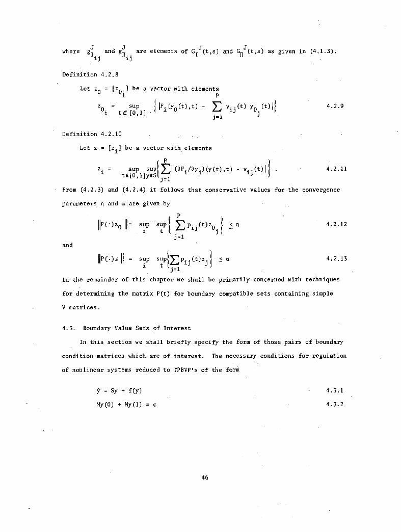
Definition 4.2.8
Let z0 = [zo.] be a vector with elements
zo.
= sup IFi (yo (t) ,t) - v. . (t) yo (t) 11te [0,1] ij
j=1
Definition 4.2.10
Let z = [z.] be a vector with elements
4.2.9
z. sup j suptEl(aF./ay)(y(t),t) - ij(t)11 . 4.2.11
ti[0,1breSj=1
From (4.2.3) and (4.2.4) it follows that conservative values for the convergence
parameters n and a are given by
P
IIP(.)z0 11= sup sup E p ij (t) z
0 I
. < n 4.2.12
33=1
and
OP(.)z sup suptEp..(t)z.} < a 4.2.1313 J
j=1
In the remainder of this chapter we shall be primarily concerned with techniques
for determining the matrix P(t) for boundary compatible sets containing simple
V matrices.
4.3. Boundary Value Sets of Interest
In this section we shall briefly specify the form of those pairs of boundary
condition matrices which are of interest. The necessary conditions for regulation
of nonlinear systems reduced to TPBVP's of the form
ÿ = sy f(Y) 4.3.1
My(0) + Ny(1) = c 4.3.2
46
where the matrices M and N depended on the quadratic cost functional being used.
Specifically we had the following cases.
Definition 4.3.3.
For quadratic cost functionals including a terminal state penalty of the
form <x(T),Kx(T)) , the boundary condition matrices were
[ I 0m _1
0 0
0 01N =
[-K I4.3.4
Since we have rank [M N] = 2n, Lemma 3.2.8 assures a matrix V exists so the set
J = {VAN} is boundary compatible. We shall henceforth refer to set (4.3.4) as
boundary value set {1}.
Example 4.3.5.
For quadratic cost functionals which do not include a terminal penalty,
the boundary condition matrices are given as
MI di
[0 0N = L°
ol
11 4.3.6
Again rank [M N] = 2n, so a V matrix exists such that J = {V,M,N} is boundary
compatible. The set (4.3.6) shall be referred to as boundary value set {2}.
4.4. Boundary Set for Regulation with Terminal Cost
In this section the use of simple V matrices with boundary value set {1}
will be considered. The requirements for boundary compatibility of the various
sets J = {VAN} will be noted in particular.
Boundary value set {1} is given specifically as.
47
M =I 0
[0 0N[
-K4.4.1
and a general 2n x2n V matrix is represented as
V = [V11
V12
4.4.2V21
V22
The fundamental matrix for V is represented as
[211(t's),$) =
212(t's)14.4.3
SI21(t s) a
22(t s)]
The matrix [M + N4,11(1,0)] is now formed explicitly as
I 0 4.4.4M+N(t
v(1,0) =[
-K011(1'0)+0
21(1,0) -K0
12(1'0)+0
22(1,0)1
and the inverse, if it exists, may be written as
[M+NOV(1,0)]-I =
[-EK012(1'
0)+022(1,0)]-1[-K011(1,0)+021(1)].
0
[-Kg12(1'0)+Q
22(1'0)]-1
4.4.5
For this inverse to exist, the matrix FIGE12(1,0)
+n22(1,0)] must be nonsingular.
It is noted that for V equal to the zero matrix or a diagonal matrix, the set
J = {VAN} is boundary compatible. The core of the Green's function is given
by the matrices [M+101/(1,0)] IM and [M+Ntv(1,0)]
-1 N which are explicitly given as
48
[M+N0V(1,0)]-1MI
'-f-°12(1,o)+222(1,o)]-1
[-KC/ 11(1'
0)44221)1'0)]
and
[Mi-N0V(1,0)]-1N
We shall now consider specific
Example 4.4.8.
4.4.6
-4-012 (1' 0)+O
22 (1' 0)]-1K I[-Kn
12)1'0)+0
22(1'0)]-1
4.4.7
choices for the V matrix.
Consider the choice of the simplest V matrix, i.e., assume V = O. The
fundamental matrix is then given as
I 00V (t,$) =
[ I0, 4.4.9
I .
Now using (4.4.6) and (4.4.7),
[1,44.Ncly(1,0)]-1m =
and
ol[IK
o4.4.10
0 0[M+N0V(1,0]-
{
-K I . 4.4.11
The Green's function matrices are calculated as
0]G(t' s) = (t,0)[M+N0 (1,0)]
-1 MOV(0,$) =
I
and
{I
K 04.4.12
GII(t's (t,0)[M+N0
V (1,0)]
-1Ne(1,$) -
[04.4.13
49
and the 2n x 2n P(t) matrix defined as
1
P(t) = f lei(t,$)Ids + II (t' s)lds
0
is calculated to be
[ tI 0P(t)
IK1 (1-01
where elements of 1K] are given as lkij. .1.
4.4.14
4.4.15
Example 4.4.16
The use of a p x p (2n x 2n) diagonal V matrix is now considered. Let V
be represented as
V =
1
•
.n
04.4.16
o
so the fundamental matrix is then simply
1(t-s)
4.4.17
0
• Xn(t-s)e
p1(t-s)
ie•
• ' Pn(t-s)e
50
which shall be denoted as
o(1)V(t,$) =
r11(t's)
0 R22(t,$)]
•
This yields using (4.4.6) and (4.4.7),
[M+N0V (1,0)]
-1 M =
R22(1'0)K
11(1,0)
and0
[M+N(DV(1,0))-1 N =[
--022-1(1,0)K
221(1'
The Green's function matrices are determined to be
and
o
0)
Ril(t,$) 0 1
Gi(t,$) =R
-1(1 ,0)KR (1,$) 0 ]22(t,0)0
2211
0
GII(t's) = -122(t' 0)Q
22 (1' 0)KR
11 (1' s) -
022(t,$)
In many instances the K matrix associated with the terminal cost is a
diagonal matrix. Let us now assume K diagonal with elements ki. Then using
(4.4.21) and (4.4.22), the P(t) matrix is found to be
51
4.4.18
4.4.19
4.4.20
4.4.21
4.4.22
P(t) =
ax1t
(e -1). 1
t1-1-(e
n -1)
'n
1K1
-p1(1-t)
1
X1 e (1-e )
\
Ikn I -1.1n(1-t)
e (1-e n)n
0
(1-t))111
1 -Pn(1-t)P
(1-e )n
4.4.23
Example 4.4.24.
Many nonlinear systems of interest have an underlying oscillator structure.
For this reason we shall consider a choice of V matrix containing linear.oscillator
elements. This
V -
choice is represented as
S ,1 .
i. 1 0* S I(
J (r.
k
4.4.24
0
n
where the S. arei
2
a.
x 2 matrices
co.
of the form
S. = 1 4.4.25-w. Q.
The fundaMental matrix for this choice of V is. given as
52
or
, ) =
v(t,$) =
(I)1(t s)
•
o
o
(Pk (t's)
(Pn(t,$)
/NS
011(t s)
o
where the 11)i(t,$) are 2 x 2 matrices of the form
a.(t-s) a.(t-s)1
1 ie cos w.(t-s) e sin w.(t-s)1
- sin wi(t-s)
(t,$) - (t-s) a.1(t-s)
COS w.(t-s)
4.4.26
4.4.27
4.4.28
From (4.4.5), the matrix [M+NOV(1,0)] is nonsingular if 022(1,0) is nonsingular.
We now have
where
0 cpn (1,0)]22(1'(3)= _
-a. -a.cos w. -e sin w.
-1 e 1
1 1
1Oi (1,0) =
- -a.
e ai 1sin w. e cos w.
1 1
so this choice leads to a boundary compatible set.
The Green's functions are found to be given as
53
4.4.29
4.4.30
and
GI(t's) =
Q22(t'0) A Q
11(o s)
GII(t's)
0
-022(t'0) A R
11(0's)
where the matrix A is given as
A = .4222(1'0) K
11(1'0).
The matrix P(t) is then given as
P(t) =
[11(t s)
t
[fIS1n(t,$) Ids 0
0
-Q22(t's)]
01 4
JIR22(t,0) A Q (0,$)Ids
JI5222(t's) Ids
0 0
Due to the oscillatory nature of the elements of G (t,$), the integration of
the absolute values somewhat complicates an analytic solution for P(t). However,
in a future section we shall consider approximate techniques for obtaining this
P(t) matrix.
4.4.31
4.4.32
4.4.33
4.4.34
4.5. Boundary Set for Regulation with No Terminal Cost
In this section the use of simple V matrices with boundary value set {2}
is considered. The requirements for boundary compatibility of the various sets
J = {V,M,N,} shall be noted in particular. Boundary value set {2} is given
specifically as
I 0
M 10 0N = 4.5.1
0 I
54
A general 2n x 2n matrix is represented as
V = V11 1112
V1121 22
and the corresponding fundamental matrix is given as
4.5.2
Q11(t's) Q 12(t's)(Dv(t,$) = 4.5.3
021(t's) 222(t's) •
The matrix [M+MV(1,0)] is formed as
[M+NOV(1,0)] =
[ 221(1'0) . S1
22 (1' 0)
and the inverse, if it exists, is given by
[[M+NOV(1,0)]-1 =-1 1
-Q22(1,0)0
21(1,0) Q
22(1)
4.5.4
4.5.5
For this inverse to exist, 022(1,0) must be nonsingular. It is noted that for
V equal to the zero or diagonal matrix, the set J = {V,M,N} is boundary compatible.
At this point we shall begin to take advantage of the fact that the remaining
results desired in this section may be obtained from the results of the previous
section with K equal to zero. These results are now presented for V matrices
of simple structure.
Example 4.5.6.
The first selection for the V matrix is the zero matrix, i.e., V = 0.
Using the results of Example 4.4.8 with K = 0, the P(t) matrix is given as
55
[tI 0P(t)
0 (1-t)I . 4.5.6
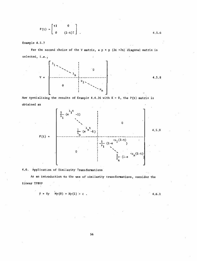
Example 4.5.7
For the second choice of the V matrix, a p x p (2n x2n) diagonal matrix is
selected, i.e.;
V -n
0
n
4.5.8
•Now specializing the results of Example.4.4.16 with K 0, the P(t) matrix is
obtained as
P(t) =
AL (e 1
t -1)
X1
0
0
-P1(1-t)(1-e
n
(l_e -pn(1-t))
4.5.9
4.6. Application of Similarity Transformations
As an introduction to the use of similarity transformations, consider the
linear TPBVP
= Vy My(0) + Ny(1) = c . 4.6.1
56
If the set J = {V,M,N} is boundary compatible, the solution to (4.6.1) is given
by Theorem 3.23 as
y(t) = OV(t,0)[M+NOV(1,0)]-1 c. 4.6.2
In an attempt to ease the calculation of the fundamental matrix 0V(t,0), consider
the use of the nonsingular linear transformation
Az = y . 4.6.3
From (4.6.1) , the transformed TPBVP is given as
= A-1
VA z MAz(0) + NAz(1) = c . 4.6.4
If the set I = {A-1VA, MA, NA} is boundary compatible, the solution for (4.6.4)
may be written as
-1 -1z(t) = 0
A VA (t)[MA + NAtA
VA(1,0)]
-1 c. 4.6.5
In passing, it may be quickly shown that if the set J = {VAN} is boundary
compatible, the transformed set I= {A-1VA, MA,NA} is also boundary compatible.
With the matrix [M+N0V(1,0)] nonsingular, post multiplication by A yields the
nonsingular matrix [MA+N0V(1,0)A]. Tho fundamental matrices are related by
A-1
VAv(1,0) = A0 (1,0)A-1 so the nonsingular matrix [MA+NOV(1,0)A] may be written
A-1
VAas [MA+N0 (1,0)] indicating the transformed set J = {A
-1VA,MA,NA} is boundary
compatible. If the transformation A-1
VA reduces V to a canonical form, the
A-1
VAfundamental matrix (t,$) is of simple structure.
Now consider the nonlinear TPBVP
= Sy + f(y) My(0) + Ny(1) = c . 4.6.6
57
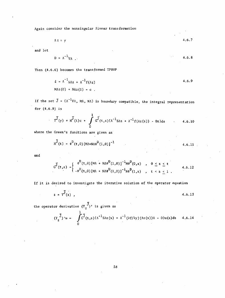
Again consider the nonsingular linear transformation
and let
A z = y
-LD = A VA .
Then (4.6.6) becomes the transformed TPBVP
= A-1 SAz + A 1f(Az)
MAz(0) + NAz(1) = c .
4.6.7
4.6.8
4.6.9
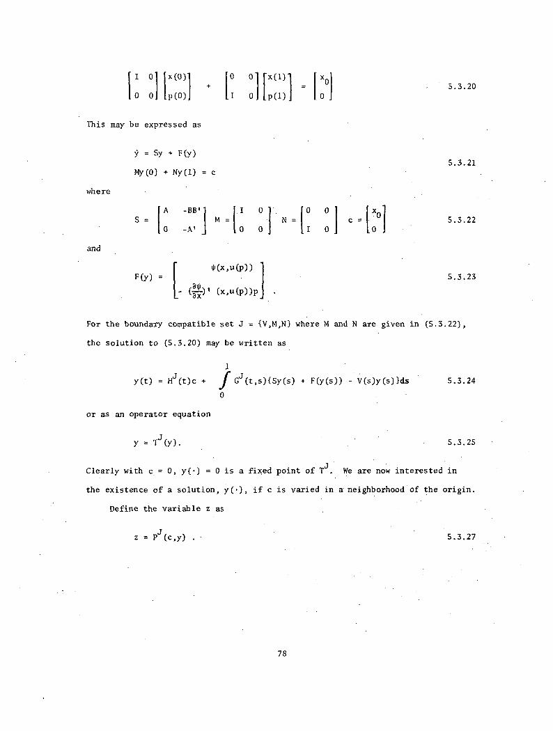
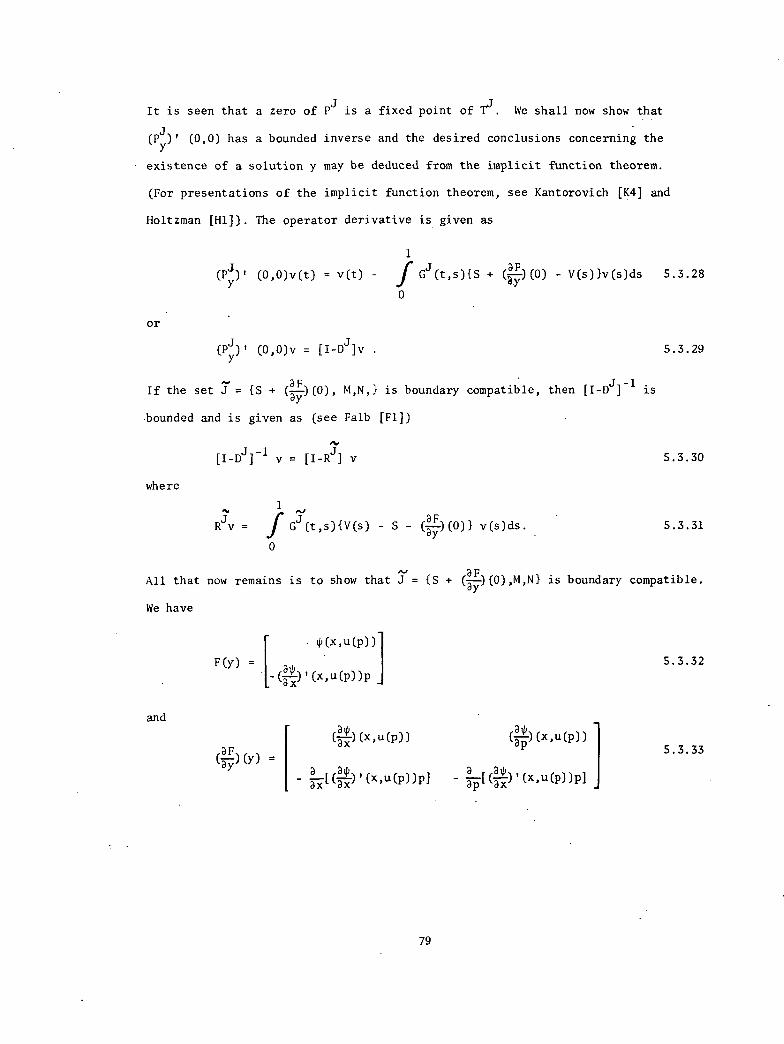
If the set j = {A-1VA, MA, NA} is boundary compatible, the integral representation
BFIf the set 3" = IS + (--)(0), M,N,} is boundary compatible, then [I-Dj]
-1 is
Dy
bounded and is given as (see Falb [F1])
where
5.3.29
[I-Dj]-1 v = v 5.3.30
1
R3
= BF
Jr. j(t,$){V(s) - S - e--)(0)1 v(s)ds.By0
5.3.31
DFA11 that now remains is to show that 3% {s (--)(0),M,N1 is boundary compatible.
By
We have
and
[
li(x,u(p))
F(Y) = a,- (i--;c) ' (x,u(p))17.
4(u)(x,u(P))
alp-
3 7,-,[(-57)'(x,u(p))pl
79
4(--)(x,u(P))Bp
D 4--4(--P(x.u(P))13]ap Bx
5.3.32
5.3.33
We have from (5.3.10) that (3Vax)(0,0) = 0 , and (atp/ap)(x,u(p)) may be
obtained as
alp alp au af(—ap)(x,11(1))) = (—au)(7-p)(x,u(P)) = -[(7-u)(x,u(P)) - BDP
which evaluated for y(.) = 0 yields
(---)(0,0) = 0 .ap
Defining the n x n matrix D(x,p) as
D(x,p) = 4P(x,u(p)) ,
it only remains to calculate
;R[D(x,p)p] and ap [D(x,p)p] .
If the n x n matrix Q(x,p) is defined as
aQ(x,p) = .57 [D(x,p)p] ,
Then the elements of the matrix are given as
and then,
n
cik(x,p) = L.
Q(0,0) = 0 .
apk,
(x,P)p-i
Similarly if the n x n matrix r(x,p) = a
[D(x,p)p]
then the elements of the matrix are given as
naDki
y .(x p) = (ap. )(x,p)pj p(x,p)ki •
j=1 1.
80
5.3.34
5.3.35
5.3.36
5.3.37
5.3.38
5.3.39
5.3.41
5.3.42
Since D(0,0) = 0 , then from (5.3.42)
r(o,o) = o .
As a result,
3F(—) (0) = 0 ,3y
and J is given simply as J = {SAN} where
A -BB'S =
0 -A' .
5.3.43
5.3.44
5.3.45
Then from the assumption that the set {A,B} is controllable and the result of
Corollary 5.2.18, the set .7= {SAN} is boundary compatible, and consequentlythe inverse is bounded. Hence for c in a neighborhood of the origin, a solution
y exists to the TPBVP and the system is null controllable in a neighborhood of
the origin as was to be proved. In addition, we note that the terminal state
is not required to be the origin, but may be any point xl in a neighborhood of
the origin.
The previous theorem does not specify the size ofir, the controllable
region, only that the system is null controllable in a region near the origin.
In addition, the condition that the linearized system be controllable about the
origin is not necessary for nonlinear null controllability. The use of the
contraction mapping theorem allows us to consider the domain of x0'
x1 such that
a solution exists to the TPBVP, and moreover, the theorem is stated without
specifying linearized controllability. As an example of the use of the contrac-
tion mappings theorem for controllability investigation, the broad class of
systems described as
81
= f(x) + Bu 5.3.46
will be considered.
Theorem 5.3.47.
Consider the control process in Rn
x f(x) + Bu in C2 in Rn x
Let yo(-) be an element of 4;([0,1],e) and let g = g(yo, . Suppose that
5.3748
(i) J = (V,M,N1 is a boundary compatible set, and (ii) there are real numbers
n and a with n > 0 and 0
1) IlTj(y0)-y0 II =
< a < 1 such that
1
(t) xol
0
+ Gj (t,$)
I 0
-V(s)
2) sup_ / 11(T;)' sup_ supyE g • y E S Hun < 1
0
af- (rip (x(s))
3) 11
<a — n r .
[-BB'po(s) + f(x0(s))1
af- (ye (xo(s))po(s)
xo(s)1 1 )(0(01ds -
PP) PO "
1
f Gj(t,$)il
0
3x
< n
(uf)(x(s))
5.3.49
[(4)1 (x(s))p(s)]
-V(s) u(s)ds <
5.3.50
5.3.51
Then the CM sequence {yil(*)} for the TPBVP based on y0 and J converges uniformly
to the uniqUe solution y* in 8 and a control exists, u = -B'p*, to steer the
82
system (5.3.48) from x0
to the origin.
Proof. Consider the optimization problem consisting of the system (5.3.48), the
cost functional
=21
1
f<u(t), u(t)> dt,
0
5.3.52
and the boundary conditions
x(0) = x0 , x(1) = 0 . 5.3.53
Application of the Pontryagin principle to the posed optimization problem
reduces the necessary conditions for optimality to the TPBVP
1 -BB'p + f(x)I
a- e-
fd ' (x)p
I 01 lx(0)1 [0 0.1 [ x(1) }
0 0 p(0) I 0 p(1)
5.3.54
5.3.55
For the boundary compatible set J = {VAN}, the solution to the TPBVP may be
written under certain smoothness conditions as
lx(t) 0
] Tj(y)(t) = Hj(t) [x
p(t) 0
1
f Gj(t,$) -BB'p(s) + f(x(s))
af-t-c) (x(s))p(s)
- V (s) x(s)ds
p(s)
83
5.3.56
Applying contraction mappings Theorem 3.4.14 to the operator (5.3.56) yields
the conditions to be proved in Theorem 5.3.47.
For the general system formulation, k = f(x,u), the canonical equations
of 2.3.54 are used subject to the boundary conditions (5.3.55). Techniques for
calculating the criteria of Theorem 5.3.47 will now be considered.
5.4. Evaluation of Controllability Convergence Parameters
In Section 4.6, the variables z0'
z, and P(t) were defined such that coarse
estimates for n and a were obtained as
andn =
• a = .017(.)z .
5.4.1
5.4.2
In this section we shall consider the determination of z0, z, and P(t) for
the controllability Theorem 5.3.47. In particular, the conditions for boundary
compatibility and the use of simple V matrices and similarity transformations
will be considered.
The boundary value set for controllability problems is given as
oN =I oi
Assuming a general form for the .2n x 2n V matrix and the fundamental matrix
OV(t,$), i.e.,
[ V =
V11
V12
v v21 22
211(t's) C12(t's)v(t,$) =
The matrix [M+NOV(1,0)] is obtained as
84
1 221(t's) C122(t's) '
5.4.3
5.4.4
be used in the integral representation.
[M+NOV(1,0)] is given as
[M+10V(1,0)]-1 =
I
If det[212(1,0)]
1
0 ,
-1 2) 2-212(1 '11' (12) D (112 '
0)1
and then the core matrices of the Green's function are given as
and
o[wisloV(1,0]-11,4
-1-4.212
(1,0) 5211(1,0) 0
[[M+N(01(1,0)]-1N4Y(1,0) =
0 0
Q12 (1' 0)
11 (1' 0) I
[M+NdY(1,0)] =SI11(1'0) 52
12(1'0) .
5.4.5
This yields det[M+NOV(1,0)] = det[5212(1,0)]. Hence the condition for boundary
compatibility reduces to the nonsingularity of D12(1,0). In passing, it is seen
that neither the zero matrix nor a diagonal matrix (nor a modified diagonal) may
the inverse of
5.4.6
5.4.7
5.4.8
Since the boundary value set (5.4.3) disallows the use of particularly simple
V matrices, we shall consider an approximate technique for calculating Gj(t,$)
and P(t) for V matrices of general structure.
Example 5.4.9.
Using the canonical transformation
D = A-1
VA ,
85
5.4.10
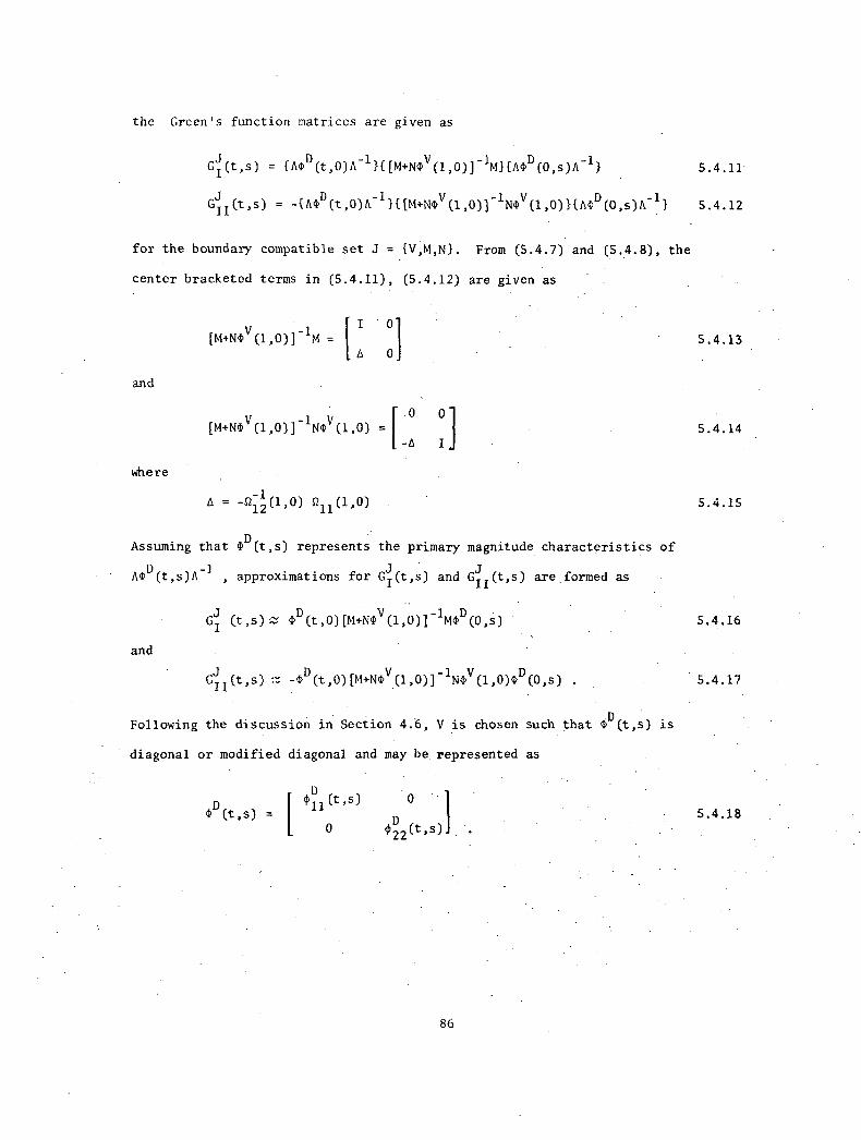
the Green's function matrices are given as
G/(t,$) = {A(1)D(t,0)A-1
}{[M+N(1)V(1,0)]-1M}{A~D(O,$)A-1}
GII(t's) = {Ad?D(t,O)A
-1 }i[M+N(01(1,0)] 110V(1,0)}(A(1)
D(0,$)A
-11
5.4.11
5.4.12
for the boundary compatible set J = {VAN}. From (5.4.7) and (5.4.8), the
center bracketed terms in (5.4.11), (5.4.12) are given as
I 0[M+N(01(1,0)]-1M = 5.4.13
and
A 0
0 0[M+N(DV(1,0)] 1N4Y(1,0) = 5.4.14
where
-A I
A = -5212
1(1' 0) 52
11 (1' 0) 5.4.15
Assuming that (I)D(t,$) represents the primary magnitude characteristics of
AOD(t,$)A
-1 , approximations for G
I(t,$) and GII(t,$) are formed as
G, (t,$)D(t,0)[M+10
v(1,0)]
-1 /0
D (0,$)
and
5.4.16
Gj (t,$)D(t,0)[M+N(1) (1,0)]-1N(IY(1,0)(1)
D(0,$) . 5.4.17
Following the discussion in Section 4.6, V is chosen such that e(t,$) is
diagonal or modified diagonal and may be represented as
D 4)11(t,$)(t,$) = 5.4.18.
0 4)22(t's)1 •
86
Using this form of 0(t,$) in (5.4.16) and (5.4.17), the approximations for
yt,$) and G11(t,$) are given as
and
D011(t,$) 0
0D 2 1 (t,0) tap
D 1(0,$) 0
0 0
GII(t's) DAO
11(0,$)
4)22(t'O) °22(t's)1
The approximation for P(t) is then given as
where
P(t);;,-
- tfl D011(t,$)Ids0
(t,0) Aell
(0,$)Ids
A = -5212(1'0) 52
11(1,0) .
0
1
f l(pD22(t ,$) Ids
t
5.4.19
5.4.20
5.4.21
5.4.22
For D a diagonal matrix, P(t) given by (5.4.21) becomes a particularly simple
form. Several variables are now defined which will be used with P(t) to calculate
estimates for n and a in Theorem 5.3.47.
Definition 5.4.22.
Using the boundary compatible initial estimate, y0(t) = Hj(t)c, define the
2n vector z0
as
87
[
1-BB'p0(s) - V11x0(s) -
V12p0(s) + f(x0(s))1
z --. sup 5.4.23
I -V21x0(s) v22p0(s) - ofl2xF(x0(s))po(s)1
A conservative estimate for n is given as
n = HP(.)zo . 5.4.24
Definition 5.4.2S.
Define th erealnumbersv,Eand
vi4 = supixe51`3x.'`
asij ij, Gij
ir 3f„• iVll..l
5.4.26l i
x) - j=1- • 'n
"3
Ei=1(-1313')
ij
and
..aij
= sup
- V12.
1 ; i,j=1,nj
ij
n 2f
I ILE]
-5.4.27
5.4.28(axl .)(x) Pk' '
x,pe S k=1
and define the n vectors zI and z
II to be composed of the elements
n
(v . ij . + E .
1). ) 5.4.29
j=1
and n
zII.
= I: ij
5.4.30
j=1
Then the 2n vector
z =1 z
IzII
z defined as
,5.4.31
88
may be used with P(t) to obtain a coarse estimate for a as
a = .
Numerical evaluation of the convergence criteria is presented for various
examples in Chapter 6.
-89
:
5.4.32
. Page Intentionally Left Blank
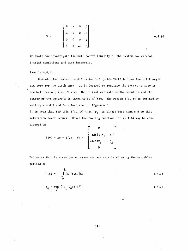
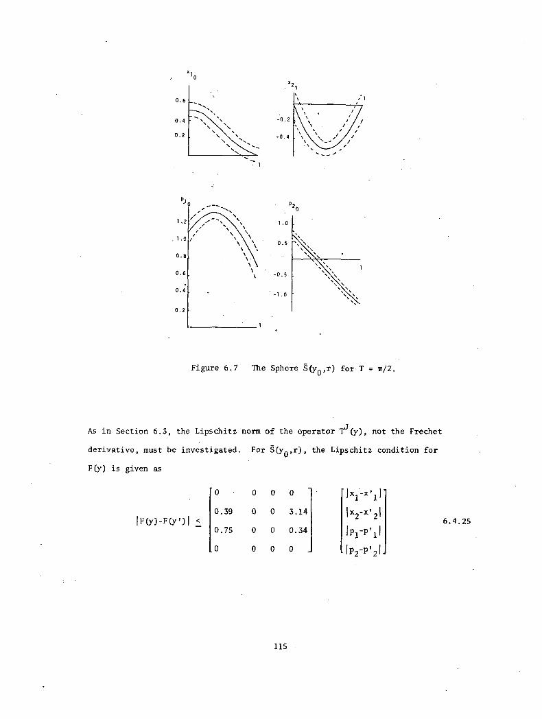
CHAPTER 6
ITY ICAL EXAMPLES
6.1. Introduction
We examine the regulation and control of several nonlinear systems to
demonstrate the usefulness of contraction mappings and to illustrate the practical
applications of the major theorems. There are many well known and very powerful
iterative methods for the solution of optimal control problems. However, practical
convergence criteria are few and far between. In this chapter we demonstrate
that general results may be obtained via the application of the contraction
mappings convergence theorem. In addition, the practical application of the
contraction Mapping algorithm demonstrates that in many cases it is an efficient,
straightforward technique for the solution of optimal control problems. The
examples demonstrate that practical application has a much broader range than
the theoretical results might imply. This is primarily due to the coarse
estimates which are used to evaluate the convergence parameters.
The first example to be considered is the regulation of the well known
Van der Pol equation. As an illustrative exercise, both contraction mappings
and modified contraction mappings are applied to this problem. The results
obtained are compared with previously published data. The second example
begins a two part sequence investigating the null controllability of nonlinear'
systems. The first member of the sequence is a particularly simple system
which serves to introduce bounded control problems. The final example of the
91.
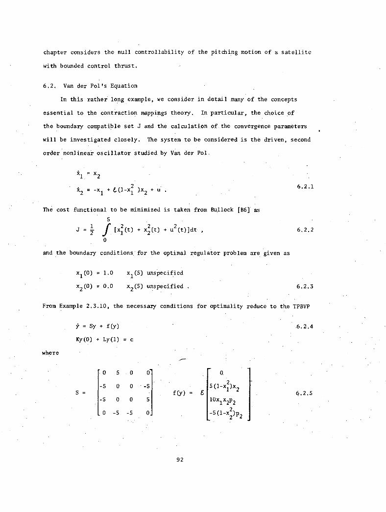
chapter considers the null controllability of the pitching motion of a satellite
with bounded control thrust.
6.2. Van der Pol's Equation
In this rather longexample, we consider in detail many of the concepts
essential to the contraction mappings theory. In particular, the choice of
the boundary compatible set J and the calculation of.the convergence parameters
will be investigated closely. The system to be considered is the driven, second
order nonlinear oscillator studied by Van der Pol.
k1 =x
2
k2 = -x
1 + E(1-x
1 )x2 + u .
The cost functional tO be minimized is taken from Bullock [B6] as
j21 2
+ x(t) + u2(t)]dt ,
and the boundary conditions for the optimal regulator problem are given as
x1(0) = 1.0 x1 (5) unspecified
x2(0) = 0.0 x2(5) unspecified .
6.2.1
6.2.2
6.2.3
From Example 2.3.10, the necessary conditions for optimality reduce to the TPBVP
= + f(y) 6.2.4
Ky(0) + Ly(1) = c
where
0 5 0 0 0
-5 0 0 -5 5(1-xl2 )x2
S = f(y) = 6 6.2.5-5 0 0 5 10x
1x2p2
_ 0 -5 -5 0, -5(1-x2
2)p2
92
and
1 0 0 0 0 0 0 0 1
0 1 0 0 0 0 0 0K = L = C = 6.2.6
0 0 0 0 0 0 1 0 0
0 0 0 0 0 0 0 1_
Using a boundary compatible set J = {V(t), M, N}, (6.2.4) may be expressed in
integral form as
y(t) = Hj(t){c-Ky(0) - Ly(1) + My(0) + Ny(1)}
1
+ f ){sy(s) + f(y(s)) - v(s)y(s)}ds6.2.7
The iterative solution of (6.2.7) by contraction mappings is now considered.
We begin with the selection of the boundary compatible set J = {V(t),M,N}.
Since the boundary conditions of (6.2.4) are linear, the natural choice
for the matrices M and N are M=K, N=L. If the initial estimate of the solution
is then chosen as Hj(t)c, every member of the contraction mapping sequence
satisfies the boundary conditions. As indicated previously, it is often
advantageous to choose the matrix V in such a way that {S + (af/Dy)(y)-V(s)}
is small. Following this guideline generally requires inclusion of time
varying functions in the V matrix, thus complicating the convergence analysis.
However, if 6 is small in (6.2.5), an acceptable choice for V is simply the
linear part-of (6.2.4), i.e., V = S. For larger values of t , it may become
necessary to include an effect of the nonlinearity in the choice of the V matrix,
but for now, consider V to be chosen as
93
o s o
-5 0 0 -51.1
-5 0 0 5
_ 0 -5 -5 0
6.2.8
The variables P(t), zo, and z, defined in Chapter 4 for use in convergence
analysis, will now be obtained for this example. From (4.2.9), (4.2.11), (6.2.5)
and (6.2.8), the vectors z0 and z are
0
15 (1-xl2 (t)0)x2(t)0 1
z0
supt 110 x1(t)0x2(t)0p2(t)0 1
Is (1-xl2 (t)0)1)2(t)01
and
z = sup sup_t yE S
. '0
xl(t)x2(01 + 1(1-xf(t))1
2(t)p2(t)1 + 12 xl(t)p2(t)
(t)P2(01 1(1-4.(t))1
xl(t)x2(t)i
6.2.9
6.2.10
for V given by (6.2.8), the calculation and structure of the fundamental matrix
is sOmewhat involved, thus complicating the calcUlation of P(t). Since the
characteristic roots of V are two pairs of complex conjugates, the techniques of
Example 4.4.24 are useful for evaluating the P(t) matrix. The canonical
transformation
= A IVA
94
6.2;11
transforms the V matrix into the block diagonal form
a1
w1
0 0
D =-w
1a1
06.2.12
0 0 02 w2
_ 0 0 -w2
a2
where al =-3.35, wi = 4.91, and a2 = 3.35, w2 = 4.91. It is then straightforward
to calculate the matrix P(t) from (4.7.1) and (4.7.2).
The parameter e is included in the example so that the general case may
be considered. In particular we are interested in determining the range of C
for which the contraction mappings theorem is valid. Before proceeding with
the convergence analysis, the sphere g(yo,r) must be defined. The initial
estimate of the solution, yo(.) is taken to be the boundary compatible initial
estimate, i.e., the solution to the linear TPBVP
or
= Vy My(0) + Ny(1) = c
y(t) = Hjr(t) c.
6.2.13
(It should be noticed that this choice for yo does not require additional
computation since the terms are necessary for the CM algorithm.) With this
choice of yo, the radius of g is taken as r = 0.1. This sphere g(yo,r) is
illustrated in Figure 6.1.
95
1
1:0
0
Figure 6.1
1
-0.5
P20
0:5
The Sphere (ycl,r)
••••.00
From (6.2.9) and (6.2.10), the vectors z0 and z are calculated as
z0
1
0.0- 0.0
2.1 5.8e z = 6 6.2.14
2.5 12.6
3.8 7.9
Conservative estimates for the convergence parameters n and a are obtained as
and
n = sup{P(t)z0} = 2.1 e 6.2.15t
a = sup{P(t)z} = 6.76 6.2.16t
96
Using (6.2.15) and (6.2.16), the requirements of Theorem 3.4.14 are specified as
and
6.7C < 1 6.2.17
2.1 C< 0.1
1-6.7E —6.2.18
Analysis of (6.2.17) and (6.2.18) shows that for 6 < 0.034 theconvergence
conditions of the theorem are satisfied.
The case for = 1.0 is treated in the paper "A Second-Order Feedback
Method for Optimal Control Computations", by Bullock and Franklin [B6]. In
the paper, the optimization problem presented by (6.1,2,3) is solved by the
techniques of steepest descent and second variation. We now consider the
application of contraction mappings to (6.2.4) with C = 1.0. Again the V matrix
is chosen V = S. Now rather than taking yo as the solution to the linear TPBVP,
y0(t) shall be given by the fifth iteration of the CM algorithm begun with the
initial guess Hj(t)c. This choice for yo is made so that the region Š(Y0,T) is
more likely to include the solution y(t) to the nonlinear TPBVP. We again take
r = 0.1. This sphere is illustrated in Figure 6.2.
We shall first determine the convergence rate factor a. Taking the supremum
over Š, z is given as
z =
97
0
1.0
2.0
x20
-0.5
P20
Figure 6.2 The Sphere g(yo,r)
and a coarse estimate for a is
a = sup{P(t)z} = 6.8 6.2.19t
With a > 1, the conditions of the theorem are not satisfied and convergence is
not guaranteed by the theorem. However, these theoretical results are only
guidelines for the practical application of contraction mappings. In fact,
98
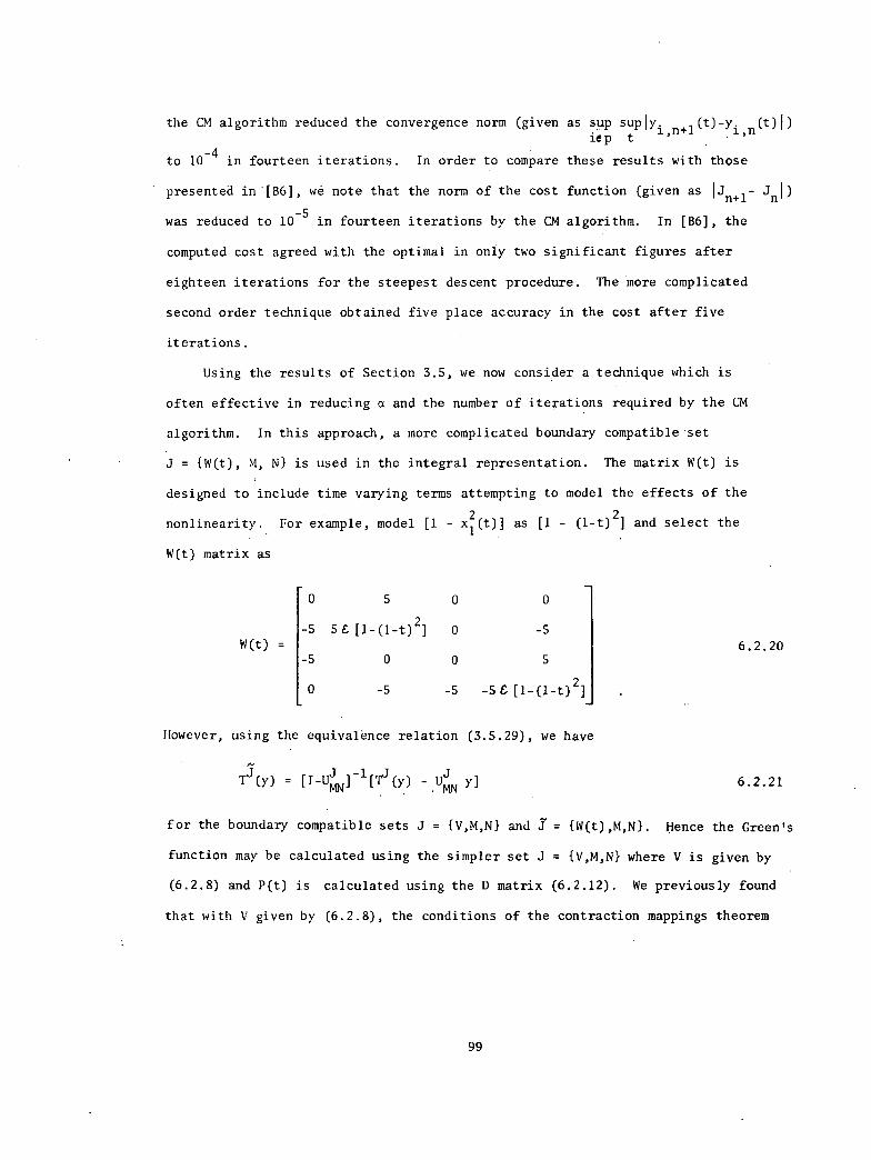
the CM algorithm reduced the convergence norm (given as sup suP1Yi n+1 (t) -Y-1 n (t )1), .,iep t
to 10 4
in fourteen iterations. In order to compare these results with those
presented in [86], we note that the norm of the cost function (given as 1J114.1
was reduced to 10-5
in fourteen iterations by the CM algorithm. In [B6], the
computed cost agreed with the optimal in only two significant figures after
eighteen iterations for the steepest descent procedure. The more complicated
second order technique obtained five place accuracy in the cost after five
iterations.
Using the results of Section 3.5, we now consider a technique which is
often effective in reducing a and the number of iterations required by the CM
algorithm. In this approach, a more complicated boundary compatible set
J = Mt), M, N} is used in the integral representation. The matrix W(t) is
designed to include time varying terms attempting to model the effects of the
nonlinearity. For example, model [1 - x12(t)] as [1 - (1-0
2] and select the
W(t) matrix as
0 5 0 0
-5 5 & [1-(1-t)2] 0 -5
-5 0 0 5
0 -5 -5 -5 E [1-(1-t)2]
However, using the equivalence relation (3.5.29), we have
W(t) =
J T3(y) = [I-U ]
-1 [1J
(y) - Uj
y]MN MN
6.2.20
6.2.21
for the boundary compatible sets J = {VAN} and = {W(OAN}. Hence the Green's
function may be calculated using the simpler set J = {V,M,N} where V is given by
(6.2.8) and P(t) is calculated using the D matrix (6.2.12). We previously found
that with V given by (6.2.8), the conditions of the contraction mappings theorem
99
are satisfied for 6 < 0.034. A similar analysis is now
The vectors z0
and z are given as
0
done for .7= {w(t),m,N}.
15x2(t)
0[1-x
12 (t)
0) - (141-0
2
z0 = sup
t110x1(00x2W0p2(001{
15p2(t)0[1-x12 (00) - (1-(1-t)
2)]I_
6.2.22
and0
12x1(0x2(01 + 10-4(0) - (1-0-02)1
z = sup {yEs 1 2x2(0132(01 1 2x1(t)p2(t)1 + 12x1(t)x2(t)1
12x1(t)p2(t)1 + l(1-xf(t)) - (1-(1-t)2)1
6.2.23
Now using = {w(t), m, N} with yo(t) = 0(t)c, r = 0.1, we find following
Example 3.5.25 and (6.2.22), (6.2.23) that conservative values for the convergence
parameters are
and
n = sup {P(t)zio} = 0.64Ct
a = sup {P(t)z} = 5.OEt
The requirements of Theorem 3.4.14 are then
and5.0C < 1 6.2.24
0.64C 0.1. 6.2.251-5.0C —
100
Analysis of (6.2.24), (6.2.25) shows that the convergence conditions of the
theorem are satisfied for
E< 0.092 6.2.26
a three fold increase over the previous value. These results are guidelines,
but indicate the improvement due to use of the better designed, though more
complicated, W(t) matrix.
Using the boundary compatible set 7 {W(t),M,N} for I = 1.0, a conservative
value for a is a = 5.1, an improvement over (6.2.14), but again violating the
theoretical specifications. However, the practical application of the CM
algorithm reduced the convergence norm to 10-5
in eight iterations, a significant
improvement over the algorithm using J = {V,M,N}. The iterative sequence for
the control function is shown in Figure 6.3.
Figure 6.3 Control Iterations
(Numbers indicate iteration sequence.)
101
A comparison of the convergence behavior for J and Xis shown in Figure 6.4.
NORM
101
100
10
10-2
- 10-3
10-4
10-5
10-6
1 3 5 7 9 11'. 13 15
NUMBER OF ITERATIONS
Figure 6.4 Comparison of Performance for Contraction
Mappings and Modified Contraction Mapptions.
6.3. Null Controllability with Bounded Control
The first example of system null controllability involves a simple linear
system with bounded input control. The example is included primarily as an
introduction to the techniques of dealing with a bounded control. Consider
the system
= Ax + Bu 6.3.1
102
where
A=10 1
1 0 0B =
[O16.3.2
and the control magnitude is constrained to.satisfy
lu(t) < 1 , 0 < t < T . 6.3.3
The initial conditions are
x1(0) = 1 , x2(0) = 1 ,
and the final state of the system is required to be the origin, i.e.,
xl(t) = 0 , x2(T) = 0 , 6.3.5
where T is a prescribed fixed terminal time.
The linear system (6.3.1) is clearly controllable since rank [B,AB] = 2.
However there do exist combinations of T and x0
such that the system cannot
be driven to the origin by the bounded control in time T, We shall investigate
the null controllability of this system by considering the optimization problem
composed of the system (6.4.1), the cost functional
T
J = 2 f u2 (t)dt, 6.3.6
0
and the boundary conditions (6.3.4),(6.3.5).
Analytical investigation of this optimization problem yields the
information that the minimum time required for the system to be driven from
(1,1) to the origin is 1 +47, and at this value, the H-minimal control is
bang-bang. As T is increased from 1 + 4T, the optimal control becomes a
103
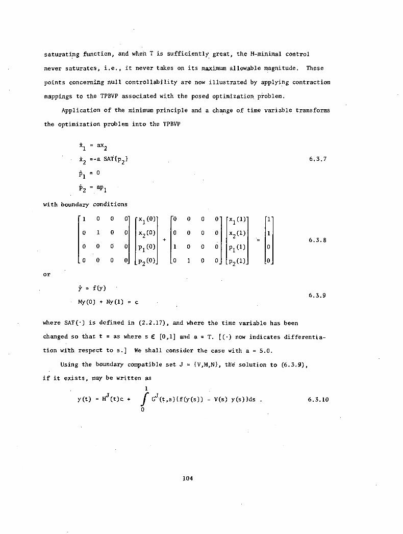
saturating function, and when T is sufficiently great, the H-minimal control
never saturates, i.e., it never takes on its maximum allowable magnitude. These
points concerning null controllability are now illustrated by applying contraction
mappings to the TPBVP associated with the posed optimization. pioblem.
Application of the minimum principle and a change of time variable transforms
the optimization problem into the TPBVP
ax21
i2 =-a SAT{p2} 6.3.7
1)1 = 0
P2 =ap1
with boundary conditions
1 0 0 0-xl(0)
0 0 0 0 x1(1)- 1
0 1 0x2(0)
0000 x2(1) 16.3.8
0000 p1(0) 1000 p1(1)0000
P2(0)-0 1 0 0_ 132(1)- o_
or
= f(y)6.3.9
• My(0) + Ny(1) = c
where SAT(•) is defined in (2.2.17), and where the time variable has been
changed so that t = as where s E [0,1] and a = T. [(.) now indicates differentia-
tion with respect to s.] We shall consider the case with a = 5.0.
Using the boundary compatible set J = {VAN}, the solution to (6.3.9),
C THF NONLINEAR EQUATION IS A FuNCTION OF THE.' STATF AT THU CuPRENTC TIME. A VECTOR np THF STATE AT THE NOT IS CREATED ANC IS usFn TOC CALCULATE F AT NOT.
10? 9F0XT(1,J)=0.000GAIN=DCOS(0.3600*X2)DGDP=-0.3600*DSIN(0.1600*X21AOD=50.0001F(X3 .GT. 10.000) GO TO 110AE0M=.75D0+.2500*DCOS(PI*v3/10.0001DFOXT(3,1)=-(.2500AtPI/10.000)*DSIN(PI*X3/10.000)*X1/A00Gn TO 111
1.10 AFOM=.5000OF0XT(3,11=0.000
111 CONT1NUFIF(X1 .GT. 60.000) GO TO 112AAM=.5D0+.500v0SIN(P1*(X1-AVB/2.0001/AVB)DROA=GAIN*X2*.500*(PI/AVB)*CCOS(PI*(X1-AVB/2.0D0)/AVB)GO TO 113
SUBROUTINE. DIFEON,PMODE,T,OTICTRiVAR,RHSIC THIS SUBROUTINE IS USED rn INTEGRATE FOR PHI AND PHIS.C THF TECHNIQUE IS A FOURTH ORDER RtINGE-KUTTA AS MODIFIED RY GILL.
.2 IF(CTR) 99,3,53 CCCI=.5D0CCC2=1.D0CCC3=DT*.500T=T+CCC3GO TO 20
5 IF(CTR-2) 6,7,96 CCC1=MNUS14 CCO=CCC1
CCC3=CCC1*DTGO TO 20
7 CCC1=PLUST=T+DT*.500GO TO 14
P CCC1=.1666666666666667D0CCC2=.3133333333333333D0CCC3=DT*.500CTR=-1
20 CTR=CTR+1CCC1=CCCI*DT
DO 22 J-.=1,NUGHLY=CCC1*RHS(JI-CCC2YtOLAM(J)OLAM(J)=OLAM(J)+UGHLY+UGHLY+UGHLY-CCC3*RHS(J)
22 VARW=VAR(J)+UGHLYRETURN
99 WRITE(6,30)PETURNFND
SUBROUTINE STTRM(NDIM)C 'THIS SUBROUTINE CoMPUTES THF STATE TRANSITION MATRIX OF THE LTNEARC SYSTFM AND TTS ADJOINT AND STORES THEM AS FUNCTIONS OF TIMF.
SUBROUTINE OUTT(T,Y,NDIM)C THIS SUBROUTINE STORES THF MATRIX PHISt.,0) AT APPROPRIATE.0 INCREMENTS OF TIME.
nntiBLE PRFCISION PHI,PHIS,RHIOS,DELT,EN,D,YS,QINT,OQINT,V,CDOUBLE PRECISION XN,XMDOUBLE PRECISION T,YOnoelE PRECISION DELT,RR,TEST,DARSCOMMnN PHI(9,9,21),PHIS(919,21),DELT,FN(9,211,D(91COMMON YS(9,21,151,0INT(9,211,0MINT(9,211,V(9,9,21)cn.imrIN c(9)oN(9,9),xm(9,9),TI,ITTcrimmoN KK,LL,Nom,NINT,TTERDIMENSInN Y(9)DELT=.05D0RR=FLOAT(LL)TEST=DAPS(RR*DELT-T1IF(TEST .GT. .000100), GO TO 100WRITE(6,101) T
101 FORMAT(' ',4HT = ,015,p)
LL=LL+100 99 J=1,NDIMPHIS(III,J,LL)=Y(J)
99 CONTINUE100 CONTINUF
RETURNENO
SUP:ROUTINE CALEANDIm)C THIS IS THE MAJOR SUBROUTINE TN THE PROGRAM. HERE THE INTFGRALC EDUATIONS ARE SOLVED FOR THE ITERATED SOLUTIONS AND THF TFST EnqC CONVERGENCE IS MADE.
C THILT RELAXATION FACTOR IS READ IN. NORmALLY TT IS ONE.REAC(,555) RF
55 FORMAT(D10.2)C THE 40uNDARY CONDITION MATRICES TN THF BOUNDARY COMPATIBLEC SET J-1..(V,M,N) ARF Nnw READ IN.
nn 2 I=1,NDImREAD(5.11 (XM(I,J), J=1,NOIM)
I FORMAT(010.2)2 CONTINUEDO 4 I=I,NDIMREAD(5,3) (XN(I,J), J=1,NOIM)
3 Fop:MATO:110.21
4 CONTINUEr FPS, THE CONVERGENCE MEASURE IS NOW READ IN.
RFAO(5,q) EPS? PMAT(010.21
C THE BOUNDARY CoNOITTON VECTOR C TS NOW READ IN.RFAfl(5,10) (C11), I=1,NnTm)
10 FORMAT(D10.,1C THE CONSTANT ISM TS Nnw READ IN. IF ISM IS nNE, THE PROGRAMC CoMPUTFS THE INITIAL BOUNDARY COMPATIBLE GUESS.C. IF ISM IS NOT ONF, THE INITIAL SOLUTION- IS NOW READ TN.
READ(5,666) JSM(s6'3 FORMAT(I10)
C NOW FOPMING TUE PRODUCT OF N*PHI(1,0)Do 7 J=1,NOTMno 7 I=1,NDIMXC(I,J)=0.000DO 7 K=1,NDIM
7 XC(I,J)=XC(1,J)4-XN(I,K)=PHI(K,J,NINT)C THE MATRIX SUM (m+N*PH1(1,0)1) I s Now FoRMED.
DO P J=1,NDIMDO B I=1,NOP1
8 SI(I,J)=XM(I,J14-XC(I,J)WRITE(6,121
12 FORMAT('0',2X,2HSI)no 15 I=1,NDImOn it J=1,NOIMWRITE(6,131 SI( I,J)
C CONVFRGENCE OF THE ITERATIONIS NOW TESTED rp. 00CALL CONV(NDIM,MM,EPS)IE(MM .FQ. I) GO TO 401
909 RETURNEND
SUBROUTINE FINT(ND(M)r SUBROUTINE FTNT INTEGRATES PHI(0,S)*EN(S) FROM ZERO TO T ANDC STORES THE INTEGRAL AS A FUNCTIflN OF T, WHERE T VARIES FROM lFflC rn ONE. THESE VALUF.S ARP USED TO CALCULATE THE INTEGRAL FROM 1 To ONE.
698 DY(NOS)=DABSIYS(I,NDS,ITER+1)-YSII,NDS,ITER))C THF LARGEST ABSOLUTE DIFFERENCE IN THIS COMPONENT WILL Nnw Vc THE,. LARGEST ABSOLuTE DIFFERENCE IN THIS COMPONENT WILL NOw BE FOUND
ITG=DYII)00 699 P=2,NINTTF(DY(m) .LT. BIG) Gn To 699BIC=DY(M)
61qc? CnNTINUF70o BIGC(1)=BIG
CrN=BIGCt1)DO 7C1 1=2,NDImIEIBIGC(L) .LT. CCN) GO TO 701CON=BIGCILI
701 CONTINUEWRITE(6,755) CON
7q5 FORmATI,01,15X,3OHNORM OF FUNCTION DIFFERENCE ,D15.8)IF(cnN .LT. EPS) GO TO 999A.m=1on TO 998
999 mm=0
99R RETURN
Page intentionally left blank
BIBLIOGRAPHY
A1. Athans, M., and Falb, P. F., Optimal Control: An Introduction to the Theory
and Its Application, McGraw-Hill Book Company, New York, 1966.
B1. Bellman, R., Introduction to Matrix Analysis, McGraw-Hill, New York, 1960.
B2. Bodewig, E., Matrix Calculus, Interscience Publishers, New York, 1956.
B3. Booten, R. C., "An Optimization Theory for.Time-Varying Linear Systems with
Non-Stationary Statistical Inputs", Proc. IRE, Vol. 40, 977-981, 1952.
B4. Brunovsky, P., "On Optimal Stabilization of Nonlinear Systems", in
Mathematical Theory of Control, A. V. Balakrishnan and L. W. Neustadt, Eds.,
Academic Press, New York, 1967.
B5. Burghart, J. H., "A Technique for Suboptimal Feedback Control of Nonlinear