Measurements of the Proton Elastic Form-Factors for 1-GeV ...

SLAC-PUB-5815

Measurements of the Proton Elastic Form-Factorsfor 1-GeV/c2 ≤ Q2 ≤ 3-GeV/c2 at SLAC

Work supported by Department of Energy contract DE–AC03–76SF00515.

November 1993

Stanford Linear Accelerator Center, Stanford University, Stanford, CA 94309

Published in Phys.Rev.D49:5671-5689,1994

R. Walker et al.

UR-1305, ER-40685- 754 SLACPUB-5815

November 8, 1993

Measurements of the Proton Elastic Form Factors for 1 5 Q’ < 3 (GeV/c)* at SLAC

R. C. Walker’, B. W. Filippone, J. Jourdan t, R. Milnert,R. McKeown, D. Potterveldt California Institute of Technology, Pasadena, CA 91125

L. Andivahis, R. Arnold, D. Benton**, P. Bosted, G. dechambrier, A. Lung++, S. E. Rock, Z. M. SzaIata The American University, Washington, DC 20016

A. Para Fermi National Accelerator Luboratory, Botauia, iL 60510

F. Dietrich, K. Van Bibber Lawrence Livermore National Laboratory, Livermore, CA 94550

J. Button-Shafer, B. Debebe, R. S. Hicks University of Massachusetts, Amherst, MA 01003

S. Dasu**, P. de Barbaro, A. Bodek, H. Haradasg, M. W. Krasny***, K. Langttt,E. M. Riordan*t* University of Rochester, Rochester, NY 14627

R. Gearhart, L. W. Whitlow@ Stanford Linear Accelerator Center, Stanford, CA 94305

J. Alster Univerdy of Tel-Aviv, Ramat Aviv, Tel-Aviv 69978, Israel

We report measurements of the proton form factors, G% and Gk, extracted from elastic scattering in the range 1 5 Q2 5 3 (GeV/c)’ with total uncertainties < 15% in CL and < 3% in CPM. Comparisons are made to theoretical models, including those based on perturbative QCD, vector- meson dominance, QCD sum rules, and diquark constituents in the proton. The results for GP, are somewhat larger than indicated by most theoretical parameterizations, and the ratios of the Pauli and Dirac form factors, Q’(F,P/Ff), are lower in value and demonstrate weaker Q2 dependence than those predictions. A global extraction of the elastic form factors from several experiments in the range 0.1 < Q2 < 10 (GeV/c)2 is also presented.

PACS numbers: 13.4O.Fn, 12.38.Qk, 13.60.Fz, 14.20.D

Submitted to the Physical Review D

*Present Address: Department of Physics, University of Rochester, Rochester, NY 14627. ‘Present Address: Department of Physics, CH-4056, Basel, Switzerland. tPresent Address: Department of Physics, MIT, Cambridge, MA 02138. *Present Address: Argonne National Laboratory, Argonne, IL 60439-4843. **Present Address: Department of Physics, University of Pennsylvania, Philadelphia, PA 19104. “Present Address: California Institute of Technology, Pasadena, CA 91125. *tPresent Address: Department of Physics, University of Wisconsin, Madison WI 53706. SSPresent Address: Mitsubishi Electric Co,, Kokusai Bldg, Rm 730, 3-l-l Marunouchi, Chiyoda-ku, Tokyo 100, Japan. ‘**Present Address: IN 2P3 - CNRS, Universites Paris VI et VII, Paris, France. “‘Present Address: Department of Physics, University of Texas, Austin, TX 78712. tttPresent Address: Stanford Linear Accelerator Center, Stanford, CA 94309. fsfPreseni Address: MEC Laboratory, Daikin Industries, Tsukuba, Japan 305.

1

I. INTRODUCTION

One of the fundamental problems addressed by nuclear and particle physics over the past 30 years is the underlying structure of the proton. It has been studied using both lepton and hadron probes of increasingly higher energy, leading to the quark/parton picture of the nucleon. Elastic electron-proton scattering is a process which leaves the proton constituents bound after the collision. The cross section for this process is described in terms of two functions called the electric and magnetic form factors, CL and GL. At low momentum transfers, G$ is related to the Fourier transform of the proton charge distribution, while G$,, contains information about its magnetic moment distribution. At large momentum transfers the form factors give important information about the quark structure within nucleons, and therefore about the nature of the strong force at moderate inter-quark separation.

Elastic electromagnetic scattering of an electron from a proton, to lowest order in the electromagnetic coupling constant a, can be described by the exchange of a single photon of momentum q, leaving an electron and proton in the final state. In the laboratory frame the electron has initial energy Ec, final energy E’, and scattering angle 0; the proton is initially at rest. The mass of the electron can be ignored (Ee >> m,, E’sin2(8/2) >> m,). The four momentum transfer squared, Q2 = -q2, given by

Q2 = 4EcE’sin2(t9/2), (1)

is completely determined by the electron kinematics. The constraint that the final hadronic state contains only a single proton leads to the relation W2 = Mi, where Mp is the mass of the proton and the missing mass squared, W2, is defined as

W2=M;+2Mpv-Q2 (2)

and u E Eo - E’. The differential cross section can be written [1,2] in the Born approximation as:

Tzck = GJ,,,, 1 F.~“‘~‘(z, Q2)/v + 2 tan2(e/2)Einef(Z, Q’)/M,] (3)

where

cr* cos2(8/2) ~ott = 4Ejj sin’(0/2)’ (4)

and, Fine’(c, Q2) and F’ine’(z, Q”) are the structure functions of the proton [3] that parameterize the hadronic vertex in the scattering. The fractional longitidunal momentum of the struck partons, 2, is defined by x E Q2/2Mpv. In the elastic limit, i.e. I = 1, these structure functions are related to the Sach’s elastic form factors by:

~zF;‘=~(z, Q2)= x2G&(Q2)6(x - 1) (5)

Fine/cx, Q2), GL(Q2) + TGL(Q”),(, _ 1) 2 1+7

The elastic form factors have been normalized to G&(O) = /+ = K~ + 1 w 2.79 (the magnetic moment of the proton) and GpE(O)=l (the charge of the proton).

Integrating the cross section of equation 3 over E’, and incorporating the relations of equations 5 and 6, gives:

da dR=

where r = Q2/4Mt and e = (1 + 2(1+ 7) tan2(0/2))-’ is the longitudinal polarization of the virtual photon, which

da ( > 1 dR Molt 1 + 2Eo/M, sin2(e/2) (

G~l~~L + 2rGk tan2(e/2))

da ( >

1 1 (G; + ;G&)

dR Mott 1 + 2Eo/Mp sin2(e/2) I + r

(7)

(8) ’

at fixed Q’ is a function of 0 alone. An alternative set of form factors, referred to as the Pauli and Dirac form factors, Fp(Q2) and F,P(Q2), respectively,

can be used to describe the hadronic elastic scattering vertex. They are related to the Sach’s form factors by:

2

$‘P(Qz), G%Q2) + TG&(Q2) 1

1+7 (9)

J’,p(Q2), G&(Q2) - GpE(Q2) Kp(l+r) *

and are normalized to F;(O)=1 and F,P(O)=l. The helicity-conserving scattering amplitude is described by Fp, while Fl describes the helicity-flip amplitude.

Note the kinematic variable T that multiplies G, 2 but not Gi in equation 8. When r << 1 (small Q2), the cross section is dominated by Gk, but for r > 1, G, p dominates. This Q2 dependence is related to the fact that the magnetic force (- l/r3) dominates at short distances relative to the electric force (- 1/r2). Since it is the large Q2 regime that is of interest here, Gg is relatively more difficult to extract from the cross sections than CPM. Also note that e divides G& but not Gi. If several measurements of the elastic cross section are performed at fixed Q2 but different t, it is possible to extract both GpE(Q2) and GP,(Q2) using a Rosenbluth separation.

Since GL is only a small contribution to the cross section at large Q2, uncertainties in the measured cross sections 2 are magnified into larger fractional uncertainties in G,. In order to limit the uncertainties in GL, it was important

to maximize the range in c at each value of fixed Q2, limit statistical and random systematic uncertainties, and limit the systematic uncertainties correlated with c at fixed Q 2. This means -limiting any systematic uncertainties which are correlated with Ec, E’, 8, beam current, cross section magnitudes, time, etc., since all of these quantities change when c is changed at a fixed value of Q2.

This goal was the most important in this experiment. Previous measurements [4,5] of GL in this Q2 regime were frequently dominated by systematic uncertainties. These were usually due to uncertainties in normalization between data taken at different laboratories, or normalizations between different small- and large-angle spectrometers. In this experiment a single spectrometer was rotated around the target pivot to measure cross sections at a wide variety of angles, including intermediate angles as a check on systematic effects. In addition, improvements made to the Stanford Linear Accelerator Center (SLAC) b eamline and detectors in End Station A made it possible to substantially reduce the systematic uncertainties in the cross section measurements. These improvements included precise measurements of the incident beam energy and angle, and an understanding of the spectrometer acceptance over a wide range of E’. Improvements have also been made in the calculation of corrections for higher order radiative effects. In addition, the elastic data presented here were used to calibrate the incident beam energy as an additional check on systematic uncertainties in the deep inelastic scattering cross sections reported elsewhere [3]. A brief report of the results of this experiment were presented previously [6], and a complete description of the experiment is presented here.

II. EXPERIMENTAL APPARATUS

Most of the details of the experimental equipment are provided in the accompanying paper [3] on inelastic scattering. Additional information relevant to elastic scattering is stated here.

Energy-defining beam slits located in the “A-bend” of the accelerator just upstream of the experimental hall could be widened or narrowed to adjust the energy spread of the beam. Since the elastic cross section is a strongly varying function of the incident beam energy, and is thus sensitive to the energy distribution of the beam, the slits were kept as narrow as possible. The full-width energy spread for the elastic data was typicahy 2 0.3%.

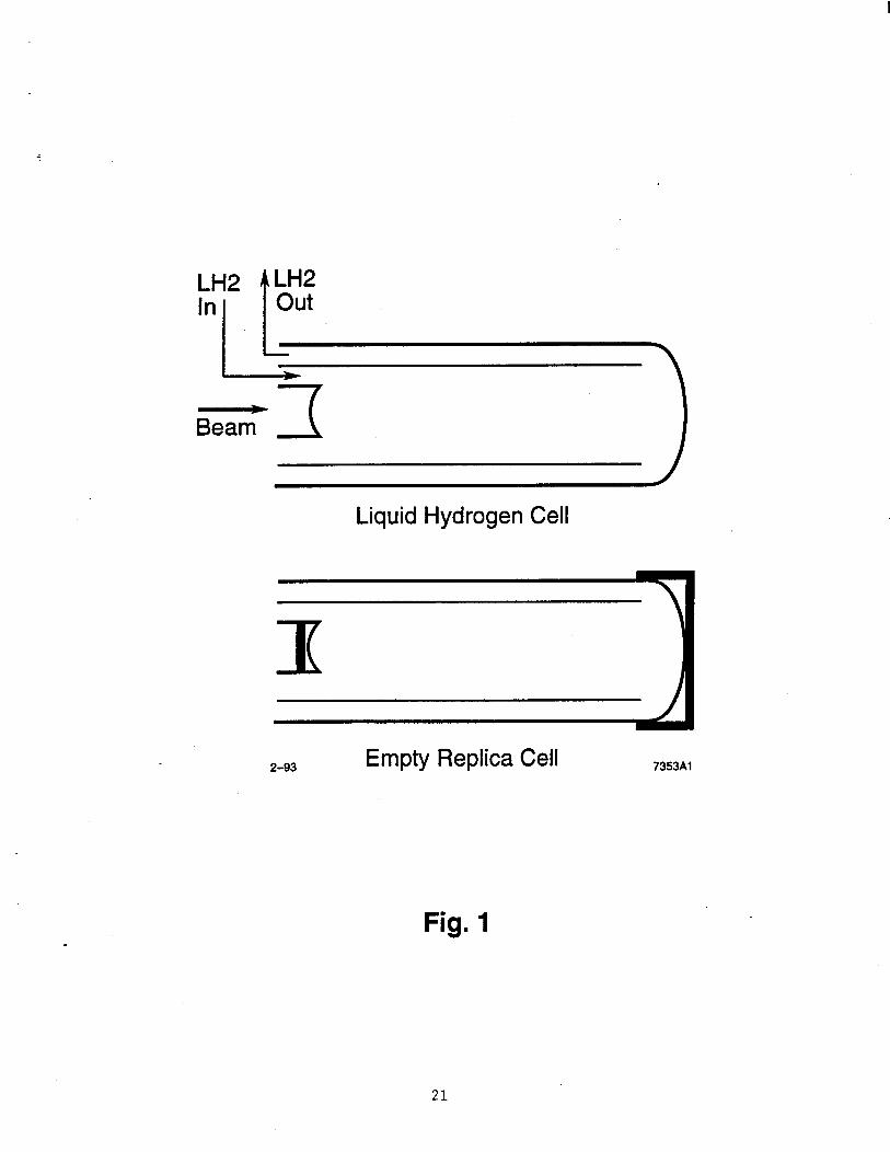
A cylindrical liquid hydrogen target (71 20 cm in length (1.41 g/ cm2) was used to scatter electrons (Figure 1). This target was 5:08 cm in diameter with side walls, entrance, and exit windows made of 0.076 mm aluminum. An identical empty replica cell with an additional 1.16 mm of aluminum radiator added to both the entrance and exit windows was used to measure endcap contributions to the scattering. The additional aluminum was added to make the thickness of the empty cell more closely resemble that of the hydrogen cell, as well as to increase the scattering rate [S].

Liquid hydrogen at 21 K and a pressure of 2 atm continuously flowed through the target. Heat deposited by the beam was removed by circulating through a heat exchanger in contact with a liquid hydrogen bath. Contamination levels within the hydrogen were measured by mass spectroscopy to be = 0.16% deuterium. A 4 cm diameter aluminum tube 0.025 mm thick was contained within the cell and was used as a flow-guide. The liquid hydrogen entered the target inside this flow-guide and exited between the flow-guide and the outer target wall. Circulation was maintained by fan-like pumps at a velocity 2 1 m/s. During the initial part of the experiment the flow direction through the hydrogen cell was in the wrong direction, causing the inner tube to bend into the beamline. The effects of this reversed flow are discussed later in this paper, and are given elsewhere in greater detail [9].

Vapor pressure bulbs and platinum resistors were located at the entrance and exit of the flow-guides to measure the temperature and pressure. The ingoing and outgoing densities were calculated from these measurements, and monitored every 10 seconds. Deviations from the nominal, beam-off, density were never more than 0.7%, and ap- propriate corrections were made. Local density changes due to heating by the beam were measured by comparing

3

electron scattering rates taken at both large and small beam currents. The effect was 0.7% at a.peak current of 37 mA, and s 0.3% at the typical operating current of 15 mA.

III. ELASTIC ANALYSIS

Experimental data from the detectors were read out electronically and recorded on magnetic tape. Two distinct steps were carried out in the analysis of these data: (1) determination of the kinematics of the scattering; and (2) measurement of the cross sections. Conversion of the data into measurements of the incident beam charge and position, electron detection efficiency, detector dead time, target density, and number of detected electrons followed a process that is detailed in the companion paper to this article [3], and will not be repeated here. Details of extraction of the elastic cross section from these data and measurement of the kinematics are discussed.

A. Kinematic Calibration

The spectrometer was surveyed and the central angle was measured with respect to the nominal beam axis before the experimental data run. During the data run, a pointer attached to the spectrometer was periodically observed through a remote video camera relative to a scribe mark placed on the floor of the experimental hall, ensuring that the angle encoder value did not change during the experiment. A more extensive survey was carried out after the data run at eight different angles from 12’ to 46”. These measurements indicated that the spectrometer angle was accurate to f0.004“. The positions of the wire chambers in the detector hut were also measured relative to the nominal central ray, and were accurate to &l mm in the wire chamber position and f0.5 mr in the relative wire chamber rotations.

A floating wire technique [lO,ll] was used to calibrate the offsets of the nominal central ray of the spectrometer. The data indicated that the nominal ray in the detector hut had an offset in the horizontal angle at the target of -0.010’. The difference between the central value of the spectrometer momentum and the nominal momentum setting was ,also measured at 14 different settings in the range of 0.5 - 9.0 GeV. Two sets of measurements with different tensions placed on the wire were in good agreement in the area of the data overlap (2-4 GeV), indicating that systematic errors were well controlled. Measurements were repeatable to f0.025%. The relationship between the magnet current and the nominal momentum setting was previously determined [12] from dark current studies done in 1967 at 3, 6, 8 and 9 GeV. A polynomial parametrization of the magnet current as a function of nominal momentum setting was used to set the spectrometer. Data from the wire orbit indicated that this polynomial gave the proper momentum selection at these momentum settings, but discrepancies as large as fO.l% still existed at other settings.

Electrons in the beam lost energy as they passed through the target material due to the ionization of atomic electrons within the target. The nominal value of the incident beam energy (and final scattered energy) was corrected for the most probable energy loss an electron would experience as it entered (exited) the target by subtracting (adding) the energy loss calculated from the equation [13-151

AEmp = O.l54(&)t [ln(1.89 x 10’(i)) + 0.1981 (11)

where t is the thickness of material in (g/cm2), Z is the atomic number of the nucleus, MA is the atomic mass of the nucleus in amu, p is the density of the material in (g/cm3), and AE,,,, is given in MeV. Agreement between this equation and a more exact, energy dependent calculation [13] was better than 0.1% for all electron energies above 50 MeV. The most probable energy loss was averaged over the target length assuming a uniform probability of scattering along the target. The typical size of this correction was 2.5 MeV. All references to Eo and E’ throughout this paper include corrections for the most probable ionization energy loss.

Offsets of the beam position and angle at the target pivot can cause offsets in the measured momentum and angle of the scattered electron in the detector hut. The SLAC computer program TRANSPORT was used to estimate the effects of beam position and angle on the various kinematic quantities measured. Only data which were taken with the beam steering operating properly are included in this analysis, so the above corrections were typically extremely small. The beam position was known at both a wire array and a microwave cavity monitor to better than fO.l

- cm. This led to a typical uncertainty in the beam position and angle at the target pivot of fO.l cm and &0.002’, respectively, causing an uncertainty of 0.03% in Ap/p and 0.002O in A8 and 4 ( see definitions below). For certain data runs the beam was deliberately displaced by 0.3 cm in either the vertical or horizontal direction. The offsets in the observed elastic peak positions for these runs were consistent with the TRANSPORT predictions.

The kinematic constraint that elastic scattering occurs at W2 = Mi was used to determine the absolute energy calibration. Details of this analysis are included in Appendix B. A systematic shift in the elastic peak positions was

4

detected when the nominal incident beam energy was used, and it was decided to recalibrate the incident beam energy by 0.07% and the final spectrometer momentum by -0.055%. Shifts of this order were consistent with the absolute calibration of the accelerator and spectrometer, and were included in the systematic uncertainties.

B. Cross Section Calculation

A three-dimensional histogram of the number of electrons detected was produced from the experimental data through a process detailed in the companion paper to this article. The three dimensions used for this histogram were: (1) the fractional momentum Ap/p, defined by E’ = p(1 + Ap/p), where p is the central momentum setting of the spectrometer; (2) the horizontal angle A8, the difference between the projected scattering angle and the central spectrometer angle; and (3) the vertical angle 4.

Elastic scattering is kinematically determined by the beam energy and scattering angle. Thus for a fixed angular bin in 110, we first integrated the three-dimensional histogram of electron counts over the $I acceptance of the spectrometer. The range of 4 integration was chosen to be -241 4 5 24 mr. Corrections were made for the fact that the scattering angle had a slight dependence on 4. Since 4 was typically 14 mr, corrections to the cross section due to this were usually small (- 0.5%).

Corrections were then made for the acceptance efficiency of each (Ap/p, AB) b in of the remaining two-dimensional histogram. The two-dimensional acceptance function was generated by integrating over 4 the three-dimensional (Ap/p, A,8,4) acceptance function measured using an inelastic data sample [3] scattered from a thin solid target. Experimental cross sections were thus obtained for each (Ap/p, Ae) bin:

(12)

where N, is the two-dimensional detected electron histogram and A is the acceptance function measured in str. The computer and electronic dead-time are C, and C,, respectively, Qe is the total incident charge, nt is the number of target nucleons per unit area, and ccc,e, is the efficiency of the electron cuts. Ator is the acceptance corrections due to the dependence of the solid angle on the projected target length and multiple scattering in the spectrometer. Monte Carlo simulations incorporating the target, spectrometer optics, apertures, and multiple scattering were performed. The resultant solid angle of the spectrometer for an elastic peak with our acceptance cuts was parameterized by:

Af& = 1 - 0.0032 sin2 f3 - 0.0042/p’.’ - 0.00025sin2 B/p’.’ (13)

with p measured in GeV, and is accurate to &O.l% over the kinematic range of this experiment. AZ,, is the correction to the acceptance due to changes in the spectrometer optics at different magnet currents. It was measured with the wirefloat technique [lO,ll]. This correction changed the absolute normalization of the cross sections by N 0.7%, and varied with the momenta setting by f0.25% over the range 1 < p < 8 GeV. Details are presented elsewhere [9].

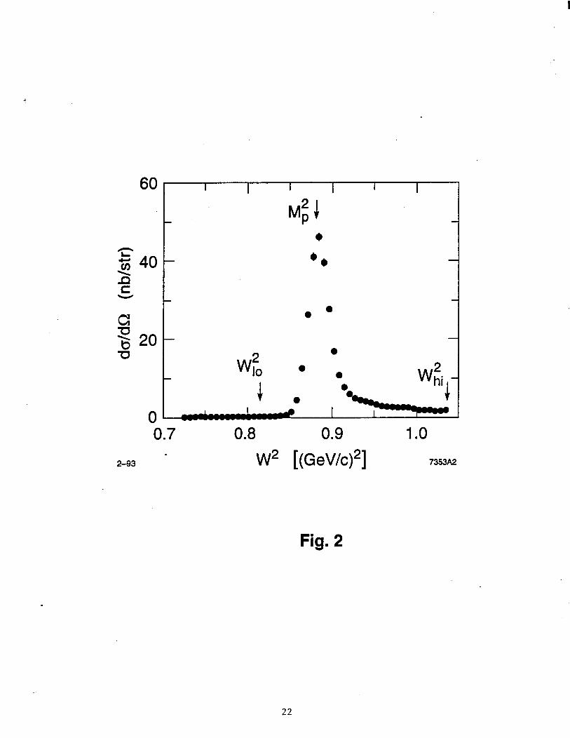
A typical elastic peak cross section is shown in Figure 2. The cross section was integrated over a suitable range in E’. The high Lip/p cut was set at a constant W2 such that the entire elastic peak was included, but as much background as possible was excluded. The lower bound of the integration was typically set at W2 = 1.12 GeV2 to include much of the radiative tail yet still exclude the pion production threshold at W2 = 1.15 GeV’. However, this cut was always set to Ap/p 1 -3% to avoid the low efficiency acceptance edges.

Cross sections in each AB bin were shifted to the value at the center of the acceptance (Ae=O) using the 0 dependence of various models of the elastic cross section (described later) including the radiative effects (see Appendix A). Final values of the extracted form factors were very insensitive to the form of this model because of the small 0 acceptance of our spectrometer. These values were then averaged across the acceptance based on their statistical weight resulting in the cross section value at AB=O. Averaging was done over a A0 range of -6 mr 5 AB 5 5 mr. Two plots of the cross section, after correction for the A0 dependence of the model cross section and averaging over a number of runs, are shown in Figure 3. No A0 dependence was found within our cuts. However, at large positive AB outside of our cuts where the acceptance is small (> 6 mr), deviations were found for runs taken at large scattering angles. Similar deviations were predicted by the Monte Carlo model of the acceptance, and were due to the effects of the projected target length not included in Afor.

It was necessary to subtract the contribution to the cross section of quasi-elastic scattering from the Al endcaps and the distorted flow-guides. The shape of the electron spectrum from Al was measured using the empty replica target. Normalization of the spectra to the full target data was determined in the kinematic domain which is allowed from quasi-elastic scattering from aluminum (due to the Fermi motion of nucleons in the Al nucleus), but is beyond

. the region of elastic scattering from hydrogen (W2 < Wi < Mi). This normalization constant was defined as:

5

Gcp = &,Wa<W:,

dRdE’ > Rep (14)

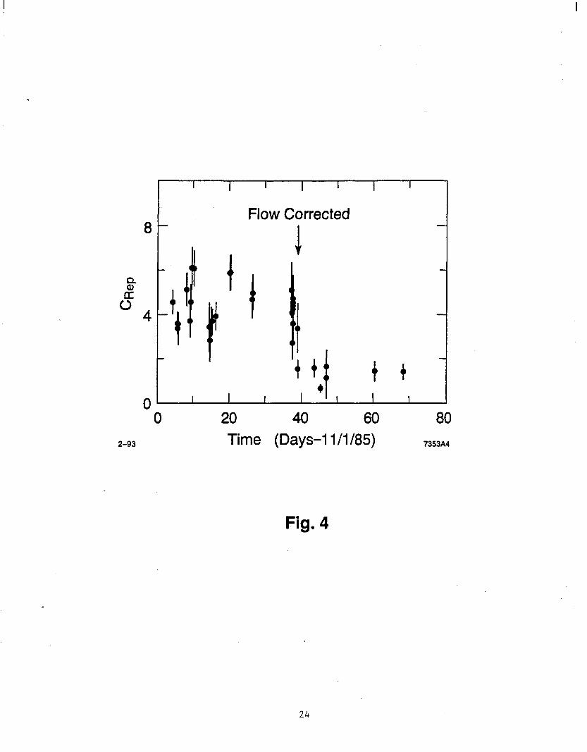
where the quasielastic cross sections have been calculated using the endcap thicknesses alone for the hydrogen and empty replica targets, respectively, and Wi indicates the cut placed on the elastic peak (see Figure 2). Figure 4 shows this normalization constant as a function of time during the experimental run. Under the conditions of the reversed hydrogen flow, the normalization constant was on average 4.43 f 0.12. Analysis of those data runs with the hydrogen flow in the proper direction gave a typical normalization constant of 1.28 f 0.12, which was consistent with the contributions expected from the aluminum endcaps and deuterium contamination in the hydrogen (0.16%).

After the determination of this normalization, the contribution of the aluminum scattering was subtracted from the scattering from the hydrogen target. Figure 5 shows some typical spectra at different kinematics in the normalization region beyond the elastic peak after the aluminum background has been subtracted. These spectra were all consistent with zero. Radiative effects due to the additional aluminum flow-guides in the beam, primarily due to bremsstrahlung and ionization losses, were also included in the calculation of the cross sections (see Appendix A). Since radiative losses tend to reduce the cross section near the elastic peak, this effect was in the opposite direction of the increased scattering from the aluminum and the two corrections tended to cancel. Both effects were proportional to the amount of additional aluminum present in the beam and thus were correlated, resulting in a smaller combined uncertainty. Typical direct contributions to electron scattering, in the elastic peak region, under the conditions of the reversed hydrogen flow was 3.0f0.3%; the typical effect of the deformed flow-guides on the radiative corrections was -2.Of0.2%. Further details of this subtraction are presented elsewhere [9].

Corrections for higher order processes in CY, which affect the scattering amplitude beyond the single photon exchange of the Born approximation, were also included. Bremsstrahlung, vacuum polarization, and vertex contributions were included as corrections to the principal scattering vertex itself, as were radiative processes within the rest of the target material. This correction was described by a parameter C’R~~, which related the measured experimental cross section to the Born cross section, sBorn:

da e=P da Born

dR = CRodE (15)

Values were in the range 0.67 < C&d < 0.78, and depended on the scattering kinematics, the lower bound of the integration over E’, and the amount of target material traversed by the scattered electrons. Significant improvements were made in the radiative correction calculations for this experiment. Details of these procedures are given in Appendix A.

Figure 6 shows the value of a typical cross section as a function of the lower Lip/p cut, normalized to the cross section at Ap/p = -3.0%. Correlations exist between the values at different Ap/p cuts. Variations in the uncorrected measured cross section were - 20% over the range of cuts shown. The chi-squared per degree of freedom (x2/df) between the cross sections evaluated with the lowest Aplpcut relative to those with the highest Aplpcut was 26.4122 for all the data runs. If systematic uncertainties due to the kinematic calibration of the elastic peak are included, the x2/df was reduced to 18.3122. This indicated a high reliability to the Ap/p-dependence of the radiative corrections and the acceptance function, as well as proper subtraction of the aluminum background.

Cross sections from different data runs but similar kinematics were weighted by their statistical uncertainty and averaged together to arrive at a single measured cross section at each kinematic point. Corrections were made for the fact that data were frequently taken at slightly different values of Q2 or c due to slight variations in the setting of the beam energy or spectrometer angle. These extrapolations were usually < l%, and were independent of the form factor model used. The typical x2/df of these averages was 1.03. Values of the cross sections at each kinematic setting, along with the radiative corrections and uncertainties, are given in Table I.

Systematic errors in the cross section measurements were estimated and included in the overall error estimate. Uncertainties in the incident beam charge, target length, scattering kinematics, spectrometer acceptance, and radiative corrections cause corresponding uncertainties in the cross section measurements. Systematic errors were divided into two types: point-to-point errors, which are different for different data runs or kinematic settings; and absolute errors, which are systematically the same for all data samples. Estimates of these errors, and their effect on the cross section measurements, are shown in Table II. The dominant contribution to the point-to-point systematic uncertainties

- was from the incident energy calibration due to the large Q2 dependence of the elastic cross section. Normalization errors of the cross sections, due primarily to uncertainties in the absolute acceptance, target length and the radiative corrections, were &1.9%. Systematic uncertainties, however, were small compared to the statistical uncertainties.

Systematic uncertainties in the radiative corrections correlated with c at a fixed value of Q2 are difficult to estimate but are expected to be small [16-181. Improvements to the data analysis could be made if a better calculation of the radiative corrections were available, particularly the terms arising from two-photon exchanges and O((r4) contributions.

6

The details of the radiative correction calculations used in this analysis have been documented [9] to allow for more precise corrections of the data as the theory of radiative corrections is improved in the future.

C. Elastic Form Factor Extraction

The relationship between the cross sections and form factors is given in Equation 8. This can be rewritten as:

1 dcBorn dred f ~(1 + r)[I + 2Eo/M, sin2(~/2)]----z

= rG& + rG;

(16)

(17)

where c was defined previously as the longitudinal polarization of the virtual photon, and the reduced cross section bred is a function of Q2 and c. A linear fit of ff,,,j to e at fixed Q2 has rGa as the intercept and G$ as the slope. Graphs of these fits to the data, including point-to-point systematic uncertainties, are shown in Figure 7, with an average x2/df of 0.62.

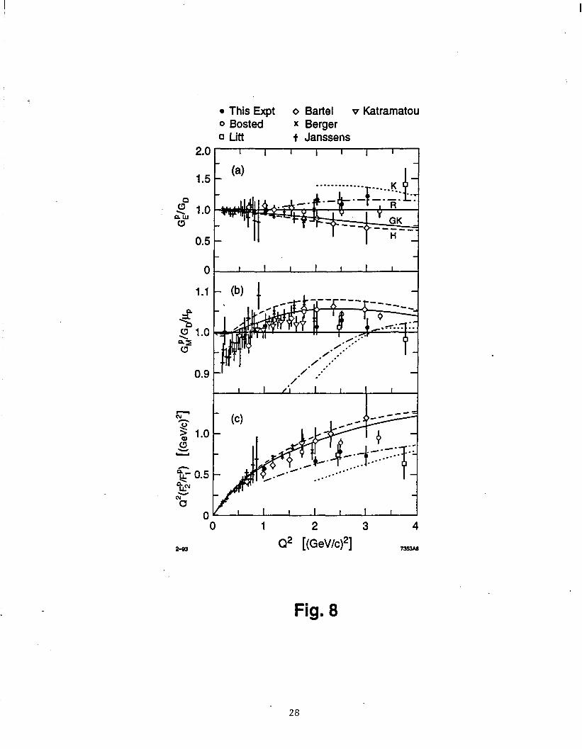
Final values of various combinations of the form factors are given in Table III. Results are also plotted in Figure 8. Values of the Sach’s form factors (G% and GR) are given relative to a simple dipole model (described later) in order to take out the dominant Q2 dependence. The ratios of Pauli and Dirac form factors multiplied by Q2 are also presented. Statistical, point-to-point systematic, and normalization uncertainties are included. The error on GE and GM are primarily due to the normalization uncertainty of the cross section and are completely correlated, but the errors vary with Q2 because of the different effects of incident energy and scattering angle. Comparisons to various theoretical models, as well as other experiments, are discussed below.

IV. ANALYSIS OF ELASTIC FORM FACTOR RESULTS

A. Global Results

1. Overview

In this section the data from selected measurements of e-p elastic scattering are presented. The experiments chosen are generally limited to those that measured cross sections at Q2 2 1 (GeV/c)2, although a significant body of lower Q2 data is also included. Comparisons are made between the form factors extracted from this work and some of the other experiments. Results of a global extraction of the form factors are presented for a wide range of Q2 values along with the relative normalizations for the different experiments.

Twelve other experiments were chosen as representative of the elastic e-p data taken in the last 25 years for Q2 2 1 (GeV/c)2. An overview of each of these experiments is presented in Table IV. All listed experiments were conducted prior to this experiment with the exception of Bosted, el al [19].

2. Comparison to Other Form Factor Measurements

Results for G~/GD, in the range Q2 < 4 (GeV/c)2, are shown in Figure 8(a) for this work and the other experiments that independently extracted Gg , i.e., Janssens, Litt, Berger, Bartel-1973 and Bosted. Our data lie consistently above the results of the other experiments, except for Litt, in the range Q2 2 2 (GeV/c)2, but all are in moderately good agreement. Uncertainties in Bartel’s results, which show the greatest disparity with the results from this experiment, were dominated by systematic errors in the cross normalization between a forward- and a backward-angle spectrometer. Janssens’ data are at too low a value of Q2 to make a meaningful comparison.

In Figure 8(b), the results for CL/GO/~, are shown for the same experiments as the GL plot, along with the data of Katramatou which only measured GL. Our data lie below the data of Bartel, Berger, and Bosted for reasons which

- are strongly correlated with the GL results. Our data are in excellent agreement with the results of Katramatou and Litt. Results for Ga are sensitive to the absolute normalization of cross sections, which have not been included in the error bars.

Figure 8(c) shows the data for Q”(Fl/Fp). Our data indicates that this combination of form factors converges to a constant for Q2 2 2 (GeV/c)2. The best fit value to the slope for Q2 2 2 (GeV/c)2 is 0.08& 0.11 (GeV/c)-2. This is in good agreement with the results of Bosted and Litt. Bartel’s results are consistently higher in value and show a

7

larger slope than our data. However, the uncertainties at the different Q2 values in Bartel’s experiment are dominated by the cross normalization of the forward- and backward-angle spectrometers, and are therefore highly correlated.

3. Global Eztraction of Elastic Form Factors

Cross section measurements from the other experiments were combined with the data of this experiment and fit for a global extraction of the form factors. From these fits, GL and Gb were extracted at 17 values of Q2, along with the eleven normalization constants between each of the experiments and this work. Cross sections were corrected for differences between the measured and nominal Q2 values using the dipole approximation. After the form factors were extracted, the fit was re-iterated using the extracted values of the form factors. Values of the extracted form factors did not change significantly. The fit was done by minimizing x2, defined by:

’ x2 z

q(i)bred(i,jr Ic) - [r(i,j)G&(Q2(j)) + c(i,j, k)Gg(Q2(j))] Kf~W&,${ 2

i=l j&l k=l Au&i, i k) (18)

(19)

where the parameters Nerpr NQz(i), and N,(i,j) refer to the number of experiments, separate Q2 bins, and different epsilon values where cross sections were measured. The values of n(i) are the multiplicative normalization constants for the other experiments relative to this work, and An(i) is the absolute cross section uncertainty given for each experiment. The cross section error bars, Au,,d(i,j, k), included both statistical and point-to-point systematic uncertainties.

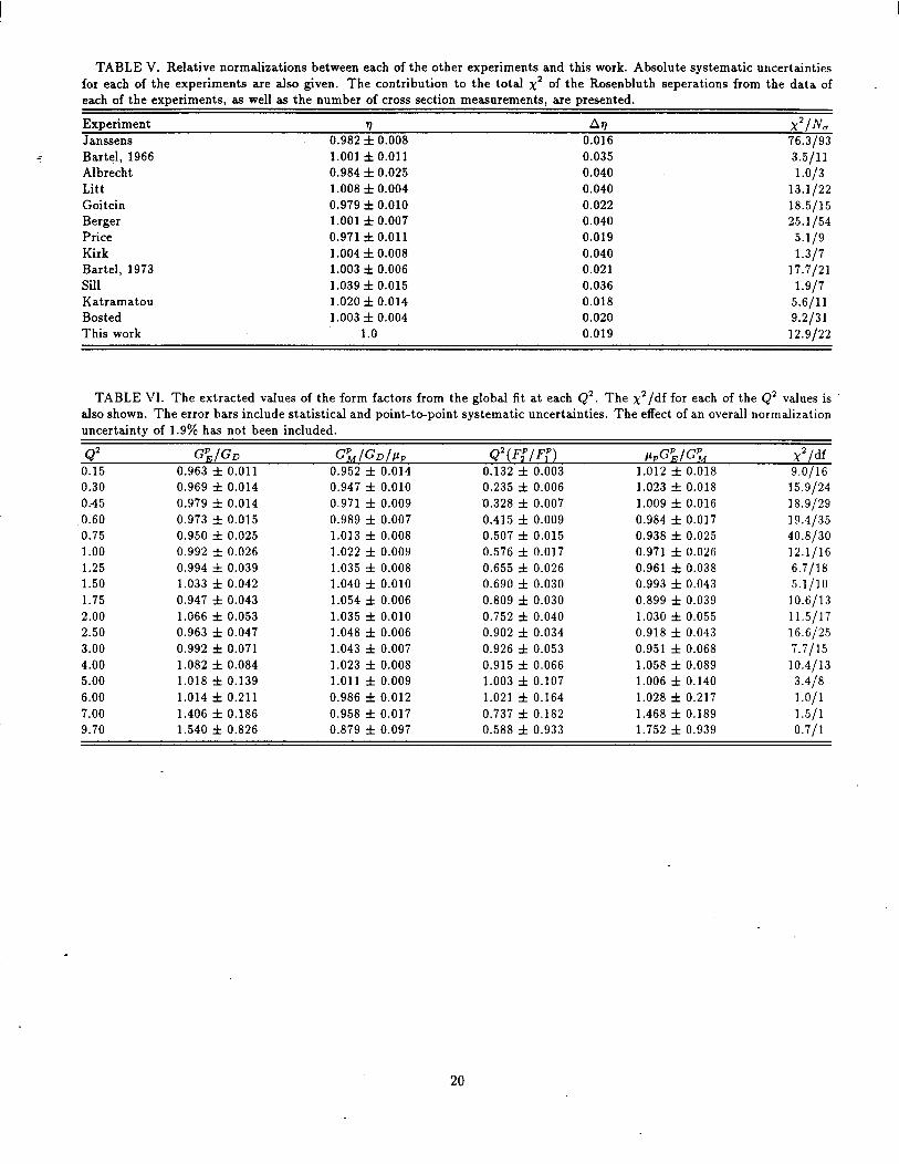
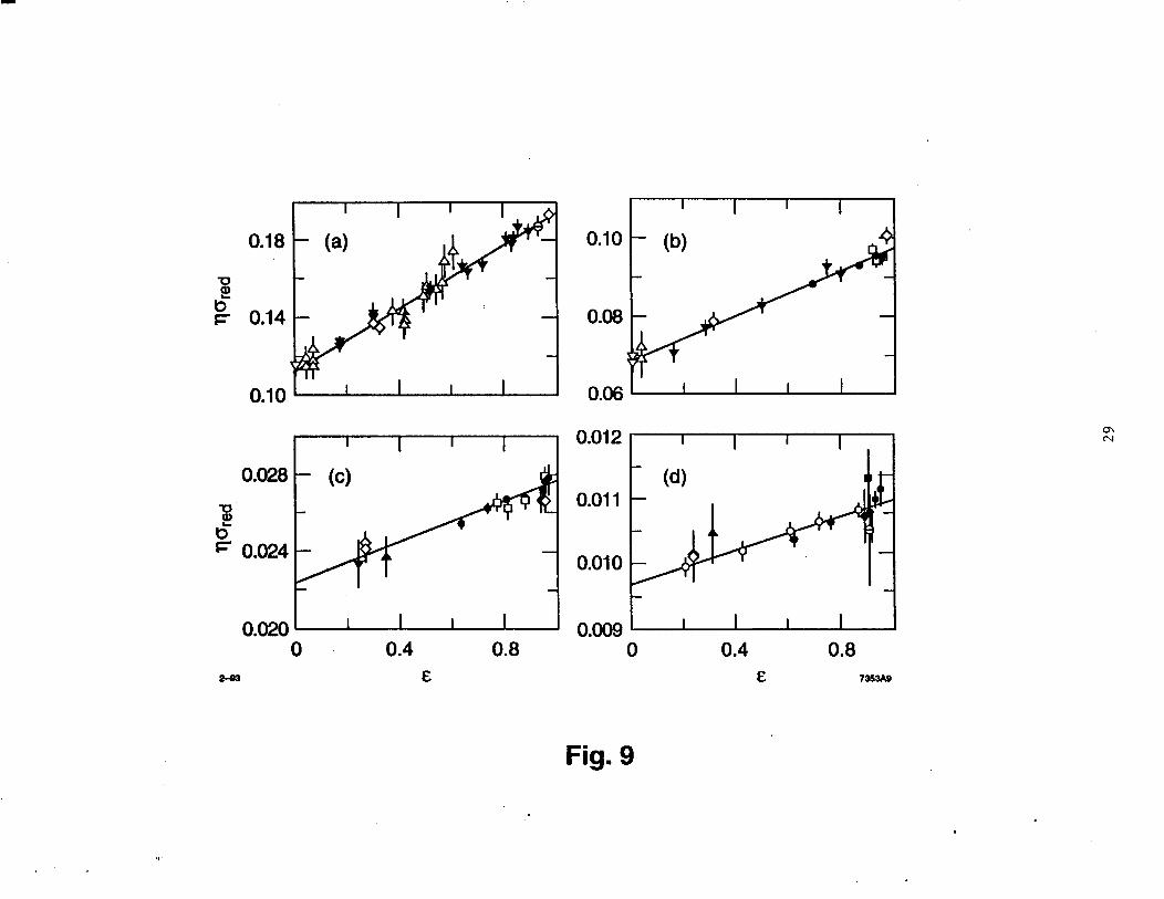
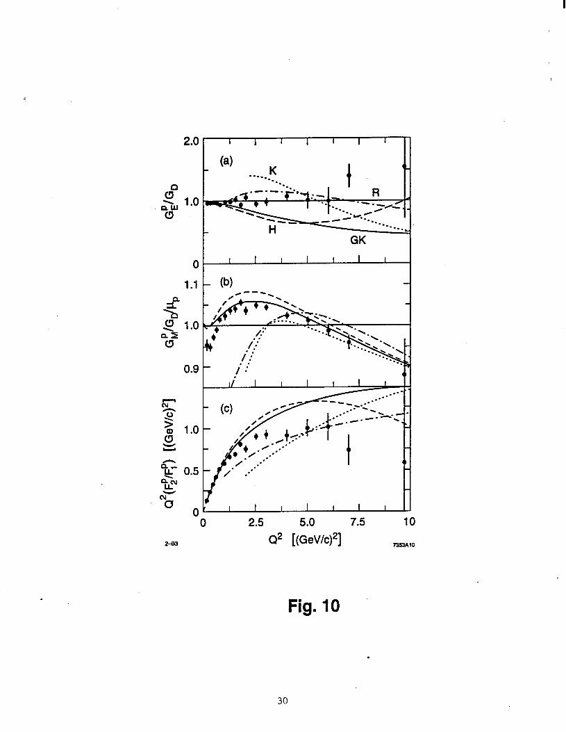
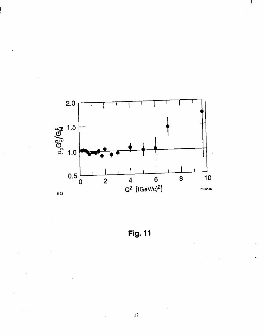
‘The total x2 for the fit was 197 for 272 degrees of freedom. A few typical c separation plots are shown in Figure ,9. Relative normalization constants for the experiments are given in Table V. Contributions to the total x2 of the Rosenbluth separations from each of the experiments relative to the total number of cross section measurements, are also presented. Values of Gg/Go, Gk/Go/p,, Q2(F.f/Fp), and p,G”,/Ga are given in Table VI at each Q2 value, along with the x2/df that was contributed from each of the Q2 points. These data are plotted in Figures 10 and 11.

The normalization constants are consistent with the systematic uncertainty assigned by each experiment. This result, coupled with the small values of x2/df for the fit from each experiment, indicates that a single normalization constant for each experiment was a good correction for the systematic differences between each of the data sets.

The data on G% are consistent with the dipole parameterization. This is in contrast to the parameterizations widely used [20] which were based on previous experimental results, and usually described Gr&Go as decreasing with increasing Q2 above Q2 = 1 (GeV/c)2. H owever, these previous results were usually - lo away from the dipole approximation, and were dominated by systematic uncertainties involved in cross normalizations between different spectrometers or different experiments. These systematic uncertainties affected the data at the different Q2 values in a highly correlated way. Data from this experiment indicate that Gg/Go does not fall significantly below 1.0 for the Q2 values measured. Results from the global extraction support this conclusion.

Values of Ga are very similar to previously published results. For Q2 < 1 (GeV/c)2 the data lie below the dipole, rising to a point that is a few percent above the dipole. At larger values of Q2 (2 5 (GeV/c)2), they again fall below the dipole, although much of the higher Q2 data taken at single c values have not been included here.

Data for Q2(Fl/Ff’) h s ow a linear rise at low Q2 (2 1 (GeV/c)2), but approach a constant at larger Q2 (X 2 (GeV/c)2). I pl t m ica ions of this behavior are discussed briefly in the following section. The data on p,Gg/Gh are consistent with the assumption of form factor scaling (G$ = GL/pp) used in larger Q2 elastic scattering experiments [21,22] to extract the value of GpM from single cross section measurements. With the uncertainties of the measurements of GpE, it is not possible to distinguish between form factor scaling and the dipole model.

B. Theories and Parameterizations

A number of different approaches have been developed to try to understand the nucleon elastic form factors. LOW Q2 data have been interpreted in terms of the spatial distributions of the charge and magnetic moment, such as the rms radius of the proton. Moderate Q2 data have been viewed in the light of vector meson dominance which models the virtual photon as a sum of massive vector mesons. The Q2 dependence of the form factors is thus caused at least in part by the Q2 dependence of the meson propagator terms. Models involving higher twist effects, such as diquarks,

8

also make specific predictions for the elastic form factors at moderate Q2. Large Q2 data have been compared to perturbative QCD predictions and dimensional scaling laws, and have been interpreted as confirmation of the quark/parton model of the nucleon and the success of quark counting rules. These various theoretical approaches, and comparisons to measurements, are presented in this section, and plotted in Figures 8 and 10.

1. Dipole Approximation and Form Factor Scaling

The dipole approximation is a lowest-order attempt to incorporate the non-zero size of the proton into the form factors. It is assumed that the proton has a simple exponential spatial charge distribution:

p(r) = Poe -r/r0

(20)

where rg is the scale of the proton radius. The form factors are related, in the non-relativistic limit, to the Fourier transform of the charge and magnetic moment distribution. If it is also assumed that the magnetic moment distribution has the same spatial dependence as thecharge distribution (i.e., form factor scaling), we get the dipole approximation to the form factors:

GdQ2k (1 + ;2r1)” (‘21)

= G’E(Q2> (22) = GL(Q2)/~p (23)

Previous measurements of e-p elastic scattering have indicated a best fit value of ri = (0.24 fm)2 = l/0.71 (GeV/c)-2, indicating an rms radius of m x 0.81 f m. better than 10% for all Q2 < 5 (GeV/c)2.

Measurements of G$ and CPM agree with the dipole approximation to

2. Vector Meson Dominance Models

Vector meson dominance models [23,24] approximate the e-p scattering vertex by assuming the primary mode of coupling between the virtual photon and the proton is through a vector meson. The form factor can be written a.s the meson propagator term times a VNN coupling term. Different models incorporate different numbers of vector mesons in the calculations, and some include a bare photon coupling in addition. The VMD model developed by G. Hiihler, e2 al. [20], incorporates terms involving the exchange of p and w mesons, plus higher terms that are associated with the 4, WI and p’ mesons. Many different fits were done to various form factor data sets. We used fit 5.3, which was the best fit to the previously available proton data.

This model (dash line in Figure 8 and 10) clearly falls below our measurements of GP, and the world extraction. However, since this theory had free parameters that were fit to previous data, slight adjustments could be made to account for the new data. In addition, due to the fact that the data on G% used to determine these parameters were available only at Q2 < 3 (GeV/c)2 (only individual cross section measurements were available at higher Q2), there are no constiraints placed on the model at higher Q2 where the new SLAC data are measured.

3. Dimensional Scaling

Dimensional scaling predicts [25] that, in the absence of an internal mass scale, the exclusive cross section of a process AB + CD can be expressed by:

,Ez $4~ + co) - s-n+2f(t/s) (24)

where n is the total number of lepton, photon, or elementary quark fields carrying a finite fraction of the momentum in the particles A, B, C, and D; s is the center of mass energy squared, t = -Q2, and f is a function of the ratio t/s. For ep + ep scattering, n = 8 and the prediction of dimensional scaling is, in the limit of large t (where Fp dominates the cross section) and fixed t/s:

9

- -+Ff Q

Therefore dimensional scaling predicts that Fp - l/Q 4 in the limit of high Q2. Since Fl is related to the helicity non-conserving part of the scattering amplitude, it is suppressed in the limit of high Q2 by a factor of - mi/Q’ relative to Fr, where mp is the quark mass scale. Dimensional scaling thus predicts that Q4Fp + constant and Q2(F;/Fr) --) constant in the limit of high Q2. This is similar to the predictions of Perturbative QCD (PQCD) [26], neglecting factors of oS(Q2) (see below).

The question as to what Q2 is high enough for QCD to be applicable is a controversial one within the literature. More discussion of this question appears in the following two subsections. Data from e-p elastic scattering [22] seem to indicate the onset of scaling (Q4F,P - constant) in the range of 5-10 (GeV/c)2. Th is experiment indicates that scaling in the ratio of the Pauli to Dirac form factors (Q2(Fl/Fr) - constant) occurs for Q2 2 2 (GeV/c)2. Data [27] on the pion form factor exhibit scaling behavior for Q2 > 1 (GeV/c)2, while neutron data [28] exhibit the behavior above 5 (GeV/c)2. Recent data [29] on the photodisintegration of the deuteron also indicate scaling at s 2 1 (GeV/c)2.

4. Perturbative QCD

M. Gari and W. Kriimpelmann [26] h ave attempted to combine the low Q2 phenomenology of VMD with the high Q2 predictions of PQCD. In this model the intrinsic proton vertex form factors, Fp and Fl, follow a monopole type behavior at low Q2, where meson physics dominates. But at high Q2 they have a dependence of Fp - l/Q4 and Fl - l/Q6 (modified by log(Q2/A2)), as predicted by PQCD. These form factors are also modified by contributions from vector meson propagator terms. For this model only the p and w mesons were included. Two parameters were introduced to define the different scales involved in the scattering; bi was the scale of the proton wave function (- 0.8 GeV) and A2 was the scale below which the meson dynamics dominate and above which the quark dynamics dominate.

This model was fit to proton and neutron form factors extracted from the previously measured electron scattering cross sections. Perturbative QCD effects begin to dominate the form factors at a value of Q2 = AZ = 5.15 (GeV/c)2.

This model (solid line in Figures 8 and 10) clearly falls below our data on GL and above our measurements of G$. As in the case of Hiihler this theory had free parameters that were fit to previous data. However, because the predictions of PQCD have been included, the behavior of the model at larger Q2 is more highly constrained. The slope of Q2(Fl/F[) of the experimental data at moderate Q2 is smaller than for Gari’s model, and the magnitude is smaller.

5. QCD Sum Rules

A model proposed by Radyushkin [30] attempts to reproduce the form factor scaling behavior that has been measured in various experiments by using only the soft components of the proton wave function and without invoking the large Q2 assumptions of scale invariance and lowest order PQCD. In this model e-p scattering is modeled as the exchange of a single virtual photon between the electron and one quark; it is then expanded in terms of o,(Q2), depending on how many gluons are exchanged between the three valence quarks within the proton. The diagram with no gluon exchanges is naively expected, based on perturbation theory, to be the dominant contribution to the form factors. At large Q2, however, 0- and I-gluon exchange diagrams are suppressed due to the momentum imbalance of the quarks and the corresponding small overlap between the intermediate state quark wave function and the final state proton wave function. Thus there should exist an energy scale, Qi, where 0-gluon exchange is dominant for Q2 < Qi, while P-gluon exchange is dominant for Q2 > Qi. Radyushkin calculates the contribution from the 0-gluon exchange diagram, and finds that it behaves like l/Q6 in the asymptotic limit. He also concludes that the.scale of Qi might be of the order of 100 (GeV/c)2, which is well above the range of presently available data which are invoked as

- an indication of the validity of the scaling model. This model (dot-dash line in Figures 8 and 10) shows good agreement with our data on Gk, but disagrees with our

measurements of Gh for Q2 5 2.5. However, the model is clearly getting nonphysical results in this region (Le., the normalization of CL(O) = pp has not been required). It also shows a flattening of Q2(Fl/Ff) that is similar to our data. Radyushkin predicts a slope in the region 2 5 Q2 < 3 (GeV/c)2 of 0.14, which is in good agreement with our results.

10

6. Diquark Models

The diquark model of the nucleon was motivated, in part, by polarized elastic p-p experiments [31] that indicated an unexpectedly large number of helicity non-conserving events in elastic proton-proton scattering. Non-perturbative effects are one way to describe such helicity flips. The diquark model of Kroll, Schiirmann, and Schweiger [32] attempts

i to include such higher twist effects. It is presumed that of the three quarks within the nucleon, two of them form a tightly coupled quasi-elementary diquark, while the third quark is more loosely bound. Diquarks can exist in either a scaler or (axial-)vector state. Helicity flip scattering amplitudes (Fl) are generated through this spin 1 diquark.

The diquark model (dotted line, Figures 8 and 10) does not describe the data in the Q2 range of this experiment (2 3 (GeV/c)2). At larger Q2, it describes the magnetic form factor extracted from the global data well; however, it does not describe the apparent flattening of the ratio of Pauli to Dirac form factors for Q2 2 2 (GeV/c)2, and overestimates the magnitude of the helicity flip amplitude (Fl) for e-p elastic scattering in this Q2 range.

V. CONCLUSIONS

We have extracted the proton form factors from e-p elastic scattering for 1 5 Q2 5 3 (GeV/c)2 using a Rosenbluth separation technique covering an angular range of cross section measurements of 11.5” < 0 5 48”. Statistical uncertainties were 5 1% in the cross sections, 7-11% in Gg and 1.5-2.5% in Ga. Improvements in experimental hardware limited point-to-point systematic uncertainties to 0.5%, much less than the statistical uncertainties in contrast to most previous form factor extractions. Significant improvements were also introduced in the calculation of radiative corrections. The absolute normalization uncertainty of the cross sections was 1.9%.

A comparison between our data and other measurements indicate marginal agreement with the DESY data but good agreement with various SLAC and Bonn experiments. Our data for GL rises slightly above the dipole approximation, while the DESY data falls about l-a below the dipole. Our measurements are also in good agreement with the ansalt of form factor scaling (GP, x Gk/p,). The measurements of Q2(Fl/Ff’) are lower in magnitude and demonstrate less Q2 dependence than the DESY and Bonn measurements.

A global extraction of the proton form factors from the data of many experiments indicates good consistency between the different data sets. These data are in agreement with the dipole parameterization of GL for all Q2 measured (Q2 < 10 (GeV/c)2), and support the ansatr of form factor scaling which has been frequently used by other experiments to extract CL from single cross section measurements at higher Q 2. The global data set strongly suggest that the ratio of Pauli to Dirac form factors, Q2(Fl/Fr), converges to a constant for Q2 2 2 (GeV/c)‘.

Parameterizations based on vector meson dominance models fall below the measurements of G$, but all have free parameters which could be refit to the more recent data. Results are in good general agreement with the predictions of dimensional scaling and perturbative QCD for Q2 2 2 (GeV/c)2. They are also in qualitative agreement with a model by Radyushkin based on QCD sum rules. A diquark model by Kroll, et al., fits the G& data well at Q2 > 4 (GeV/c)2, but does not describe the GL or Q2(Fl/Fp) results.

VI. ACKNOWLEDGMENTS

We would-like to thank B. Richter, R. Eisele, C. Hudspeth, G. Davis, J. Mark, M. Starek, J. Nicol, A. Sill and the SLAC management and staff for their assistance in this experiment. This research was supported by National Science Foundation Grants PHY85-05682 and PHY84-10549 and Department of Energy contracts DE-AC02-76ER13065, DE- AC02-76ER02853, DE-AC03-76F00515, W-7405-ENG-48, and the US-Israel Binational Science Foundation.

APPENDIX A: RADIATIVE CORRECTIONS

1. Overview

Elastic scattering does not consist of simply the one-photon exchange process outlined in the introduction. Higher order processes in Q also affect the cross section. These processes can be split into two general categories. Internal effects are those that occur as a part of the primary e-p scattering vertex, such as vacuum polarization, vertex, or internal bremsstrahlung (Figure 12). Ezternul effects are those caused by secondary scattering from rest of the material in the target, such as bremsstrahlung or ionization losses. (Figure 12).

11

These processes cause the elastic cross section to be changed from the simple B-function (smeared by detector resolution) at E’ = EL, G Ec/[l + 2% sin2(0/2)] to an asymmetric peak with an extended elastic tail at lower energies. The radiative tail extends down to values of E’ where other processes (a-production, A-resonance, etc.) also occur. Therefore, the integration of the cross section must be cut off at a value of E’ = E:, - LIE’, with the value

A of AE’ chosen to be small enough to exclude these other background processes, but large enough so that the value of the integral is not sensitive to the exact shape of the energy resolution function of the detectors.

Radiative corrections depend on the details of the target materials and geometry. They also depend in a complicated way on the kinematics of the scattering. Therefore they are included as part of the experimental corrections, so that the measured cross sections correspond to the simple one-photon exchange in the Born approximation presented in the introduction. Details of the calculation of the corrections are given below.

2. Internal Corrections

The radiative corrections procedure of MO and Tsai [16] were used to make the internal corrections for this experiment. The radiative corrections were parameterized by 6inl, which related the cross section of O(a3) to the Born cross section by:

$+x3) = (1 + &)gBorn

Higher order corrections were approximated by exponentiating 6int:

(A2)

Although this approximation was strictly valid only for the infrared divergent terms, the error caused in the nondivergent terms was estimated [16] to be small (5 0.7% at Q2 = 20 (GeV/c)2, and smaller at our kinematics).

Contributions from vacuum polarization (Figure 12(a)) and electron vertex diagrams (Figure 12(b)) were calculated explicitly. Only the infrared divergent contributions from proton vertex (Figure 12(b)) and two-photon exchange (Figure 12(c)) d ia g rams were calculated; the nondivergent components of these were estimated [16,33] to be small (< 1%). Contributions from the internal bremsstrahlung diagrams (Figure 12(d)) were somewhat more difficult to calculate. It was assumed that AE( 1 + 2Eo/M,) << E’ to simplify the calculation. Corrections for this approximation will be discussed in the next section on improvements to the internal corrections. A detailed description of the calculations involved [17] is presented elsewhere. The typical value of 6int was - -0.17.

3. Improvements to Internal Corrections

Because of the reduced systematic and statistical uncertainties of the present experiment, uncertainties in the radiative corrections at the level of x 1% caused by some of the approximations used in the previous section were unacceptably large. In calculating the value 6i,,t, it has usually been assumed that [17] the cross section did not vary significantly with AE when the internal bremsstrahlung contributions were included. This approximation is not valid to the level necessary for this experiment, and an error is introduced in calculating the contribution to the elastic tail from the first diagram shown in Figure 12(d). In this case, the electron emits a bremsstrahlung photon before scattering from the proton, giving it a lower.energy and thus an enhanced scattering cross section; by as much as 50% for the kinematics considered here. Therefore the size of the elastic tail is underestimated, and this error increases with larger values of the radiative cutoff AE.

By using the equivalent radiator approximation the effect of the energy dependence of the cross section can be estimated. Internal bremsstrahlung corrections can be approximated [16] by treating the single proton as an ezternul radiator, with equivalent radiator thickness:

biti = bftf = ~[ln(Q2/m~) - l]

These Edernul radiative corrections due to bremsstrahlung can be calculated with the equivalent radiator thicknesses. The effect of the energy dependence of the cross section can be estimated by calculating the elastic tail with s approximated with the dipole form factors relative to the same calculation assuming a constant cross section (no energy dependence). This contribution to the internal correction, afz, is defined by:

12

a!‘* e ,a* e I

dE, d%( EIJ ) E’) dipo’e dRdE’ lJ

dE, d%(Eo, E’) consr dS2dE’ (A4

This correction ranged from 0.2-3.0%, and had a strong AE’-cut and c dependence. Without this correction term, the cross sections showed a strong (- l-2%) dependence on the AE’ cut.

Vacuum polarization contributions from p+p- and qq loops were also previously neglected. We used the muon loop term:

cyo, = $[-- i+g$+(f-,, ~~)ln($(l+\/l+$$))] (A51

where M,, = 0.106 GeV is the muon mass. This contribution is the same as the electron loop contribution in the limit of Q2 >> Mi. Quark loop corrections [35] were performed using a simple fit to .this equation (with corrections for the charges and color factor) summed over all flavors of quarks, and was valid for 1 5 Q2 5 64 (GeV/c)2:

6Lc = -2(-i.513 x 10S3 - 2.822 x 10m31n(l + 1.218Q2)) (Af-3

An additional correction by Schwinger [36] was included by Tsai [18] to correct for the noninfrared divergent part of the soft photon emission cross section. A sign error in Tsai’s paper has since been corrected [37] giving the term:

6 Sch = -f [f - *(cos2(e/2))]

All these effects were then included in the definition of hi,,,:

4. External Corrections

Radiative effects that occur external to the principle scattering are caused by bremsstrahlung in the target material and the effects of the Landau tail of the ionization energy loss spectrum. Corrections were made based on the work of Tsai [18].

a. Bremsstrahlung Spectrum

An electron of energy E will emit bremsstrahlung photons in the field of a nearby nucleus. The probability of losing energy w (w s 0.8E, E 2 0.1 GeV) after passing through a thickness of 1 radiation lengths is:

q(g)=- 1- (;) + i(i)’

(A9)

(A101

where 4 is the shape of the bremsstrahlung spectrum and normalized to d(O) = 1. The parameter 6 M 4/3 is given [38] more precisely by:

b=${l+;[$$ ] [ln(184.15Z+)]-1} (All)

r,r= ln(1194Z-~)/ln(184.15Z-~) (A121

where Z is the charge of the nucleus. The cross section for an electron of initial energy Eo to elastically scatter from a proton and have final energy

Et = E;, - AE’, when the electron is emitting bremsstrahlung photons with ti and tf radiation lengths of material before and after scattering, respectively, is:

.

13

where the b-function fixes the final energy at Et = EL, - AE’, and the effect of the proton recoil is included through the parameter R which relates AEc = RAE’, (R z (B)‘). S’ mce PB(E, w, t) is strongly peaked at w = 0, the double A integral can be approximated by separating it into two single integrals; one near we x 0 and one near w’ M 0 (energy peaking approximation). These integrals can be explicitly calculated, leading to the equation:

d2u(Eo, E’) dQdE’ = (~)““‘($$J*“‘F(l :bili) I’(1 +lbfi,) (‘414)

6415)

b. Straggling and Ionization Loss Spectrum

The energy loss spectrum due to ionization for an electron of energy E passing through material in the ultra- relativistic limit is described by a Landau distribution [39] which is defined:

,$U+U I,, ” du (A161

where u > 0 is a real number. The parameter X is defined [39,18]:

A= AE - AEm, t (A17)

[= 1.54 x 10-4(Z/A)Tro (A181

where Z is the number of protons/nucleus in the material, A is the mass number, and Tzc is the thickness in g/cm’. AE,, is the most probable energy loss discussed earlier. At large X the tail of @L(X) falls like N 1/X2.

The correction for the Landau tail was small for this experiment. Under these conditions a correction to the cross section, CL, can be calculated to a good approximation by:

O” CL(AE’) - 1 - J RAE’ dwQL(K)

6 C-419)

where CL(AE/) is the fraction of the ionization spectrum that scatters with final energy E’ > Et, - AE’ (again using the energy peaking approximation), and the subscripts i and f on t refer to initial and final material thickness. The value of CL was typically 0.998 (AE’/< N 1000).

c. Calculation of Ezternal Corrections

The external radiative corrections were parameterized by a number bezr, analogous to the internal correction parameter, which is defined by relating the integral of equation A15, along with the correction for the Landau tail in equation A19, to the Born cross section:

e6.,r WEO) Born J

E:, dR

E G(AE’) dE, d2u(Eo, Et) EL, -AE’ dRdE’ (A201

The integrand on the right hand side diverges like l/(AEt)‘-** as AE’ + 0 due to the bremsstrahlung spectrum. - Therefore when 6,,t was calculated the bremsstrahlung contribution was integrated analytically in the region where

AE’ is small (EL, - Et 5 3 MeV). In this region the cross section could be treated as a constant. The contribution at larger AE’ was numerically integrated. The energy dependence of da/d0 was approximated using the dipole approximation to the form factors, but was found to be independent of any particular choice of reasonable models.

The value of 6,,, depended on where in the target the electron was assumed to scatter (through the variables li. lf, ii, and <f). It was presumed that the electrons scattered from the center of the target in the transverse direction and

14

had an equal probability of scattering anywhere in the longitudinal direction along the target. Steps of 0.5 cm were made along the target length, and the amount of material before and after the scattering, including all entrance and exit windows, etc., was calculated. The effect of the flow guides that were bent into the beam path was also included. The value of e6e=t was averaged over the length of the target. Typical values of 6,,t were N -0.18.

5. Conclusions

Combining all of the above effects, the radiative correction, C&d, is defined:

CRad G eh+L+w (A211

and corresponds to the term used in equation 15. Values of the radiative corrections at the various kinematics of this experiment are given in Table I.

Calculation of both the external and internal radiative corrections have been significantly improved by this procedure, and are in excellent agreement with the measured radiative tails of the elastic peak. However, improved theoretical understanding’of the radiative corrections could lead to even better measurements of the elastic form factors. Two photon exchange terms, which require an understanding of the contributions arising when the proton is off mass-shell in the intermediate state, need to be estimated. Explicit calculation of the 0(cr4) terms, rather than the relatively simple estimate made by exponentiating the 0(03) contribution, would prove useful. And a better understanding of the energy dependent effects arising from internal bremsstrahlung, beyond the equivalent radiator approximation used in this work, could also be important, due to the strong t dependence of these corrections.

APPENDIX B: ELASTIC PEAK CALIBRATIONS

‘The kinematic constraint that elastic scattering occurs at W2 = Mi allows a useful method to calibrate the incident ,and final electron energy. Measurements of the elastic peak positions at a variety of kinematics yields a measurement of the incident energy relative to the spectrometer momentum setting. Combining this information with the absolute calibration of the spectrometer provided by the wire orbit, an absolute calibration of the beam energy w& possible. These measurements also indicated differences between the average beam energy in a particular run and the nominal central value caused by an asymmetric distribution of the beam within the energy defining slits. A run-by-run correction of the absolute beam energy can thus be determined.

The (Ap/p, AQ, 4) histograms that were generated in the first stage of data analysis (see companion paper [3]) were converted into one-dimensional missing mass squared (W2) histograms for each run. The values of Eo, E’, and B that were used included all the corrections noted earlier. Corrections were made for acceptance effects and the A0 dependence of the cross section across the acceptance. A typical histogram measured with the hydrogen target is shown in Figure 2. Spectra from the scattering of the aluminum endcaps and flow guides were measured with the empty target replica and were subtracted from the hydrogen data.

Radiative effects, as described in Appendix A, shift the cross section from lower to higher W2. When this effect is folded in with the resolution of the spectrometer and the spread in the incident beam energy, the W2 value where the maximum of the elastic peak occurs is shifted to W2 > Mp 2. This effect must be accounted for before the peak position can be determined.

The unfolding procedure was based on the de-radiating prescription of P.N. Kirk, et al [21]. Radiative tails of the lower W2 bins were subtracted from the higher W2 bins on a bin-by-bin basis. By systematically subtracting the tails of successively higher W2 bins, the elastic scattering peak in the absence of radiative effects could be calculated. A typical de-radiated spectrum is shown in Figure 13. Note that bin-to-bin correlations exist in the values of the de-radiated cross sections. These correlations are especially strong at the higher W2 bins where a large subtraction of the elastic radiative tails has been made.

Each de-radiated spectrum was fit by a gaussian using only the 7 bins centered on the peak maximum. One bin typically had a width corresponding to a Ap/p spread of 0.1%. From these fits the gaussian height, peak position, and peak width were extracted for each run, along with their uncertainties. The typical x2/df for these fits was 0.35.

_ These small values of x2/df were caused by the correlations between the values in different bins, and thus indicated a overly conservative estimate of the uncertainties of the extracted parameters. From these measured values of the peak positions, the calibration of the incident and final energies could be carried out.

Offsets in the measured peak positions relative to the kinematic constraint W 2 = Mi can be related to offsets in any of the kinematic variables Eo, E’, or 0. However, the peak positions were very insensitive to angular uncertainties due to the high precision of the scattering angle known from the spectrometer survey, wire orbit, beam steering, and

15

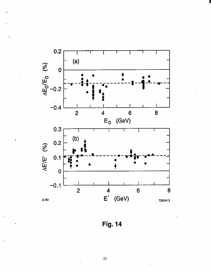
event tracking. Thus only estimates of possible incident or final energy miscalibrations were performed. The results of this analysis are shown in Figure 14. Fits were made assuming a constant, average offset in either the incident energy or the final energy. If the offsets were assumed to be entirely due to AEo/Eo, the average offset (dashed line, Figure 14(a)) was -0.15%, with a x2/df=2723/61. If the offsets were assumed to be entirely due to AE’/E’, the average offset (dashed line, Figure 14(b)) was O.ll%, with a x2/df=1614/61. These large values of x2 were caused by fluctuations of the peak positions around these average offsets, and were consistent with a typical f0.05% fluctuation in the incident beam energy. Since the full width spread in the incident beam energy was as high as 0.3%, fluctuations of this order were not surprising.

The different kinematic dependence that the offsets AEo/Eo and As/Et have on the peak offset can, in principle, allow for a two-dimensional separation of these absolute offsets. However, since the kinematic terms are highly correlated and the fluctuations in the average incident beam energy tend to be significant compared to the average offset, it was difficult to get separate constraints on both the incident and final energies. It was therefore decided to correct the final energy by -0.055% and the incident energy by +0.07%. The -0.055% shift in the spectrometer momentum was consistent with the uncertainty in the absolute calibration of the wire orbit (- 0.05%) and the accuracy of the beam steering system (- 0.1 cm). Since the cross section was only a function of the incident energy and scattering angle, shifts in the final energy had no direct effect on the measured cross sections. A systematic uncertainty of &0.07% was included in the absolute incident energy calibration to account for this incident energy correction. This uncertainty had only a small effect on the final errors on the extracted form factors.

After the absolute energy calibrations were corrected, small fluctuations in the peak positions were still observed (see Figure 15). These fluctuations were, as discussed above, consistent with - 0.05% point-to-point fluctuations in the incident energy. The incident energy for each run was corrected assuming these peak fluctuations were caused entirely by differences between the average energy of the beam and the central value defined by the A-bend slits. Point-to-point fluctuations in the beam steering system and spectrometer momentum setting could also contribute to these peak position fluctuations. A 0.03% systematic uncertainty was assigned to the point-to-point relative energy calibration to account for these possible fluctuations. This is the largest source of point-to-point systematic error (See Table II).

[l] J. D. Bjorken, S. D. Drell, Relativistic Quantum Mechanics, (1964). [2] F. Halzen, A. D. Martin, Quarks and Leptons, (1984). [3] S. Dasu, et al., UR-1260, (1993); and accompanying paper. [4] W. Bartel, et al., Nuclear Physics 58, 429 (1973). [5] W. Albrecht, et al., Phys. Rev. Lett. 18, 1014 (1967). [6] R. C. Walker, et al., Phys. Lett. B224, 353 (1989). [7] J. Mark, Advances in Cryogenic Engineering v. 30, Plenum, New York (1984). [8] A. Bodek, Nucl. Instrum. Meth 109, 603 (1973). [9] R. C. Walker, Ph.D. thesis, Caltech, 1989.

[lo] L. Andivahis, et al., SLAC-PUB-5753. [ll] L.W. Wliitlow, Ph.D. thesis, SLAC-PUB-357, Stanford University. [12] D. H. Coward, et al., Phys. Rev. Lett. 20, 292 (1968); see also ref. [21] [13] A. T. Katramatou, SLAC-NPAS-TN-86-8 (1986). [14] R. M. Sternheimer and R. F. Peierls, Phys. Rev. B3, 3681 (1971). [15] A. Crispin and G. N. Fowler, Rev. of Mod. Phys 42, 290 (1970). [16] L. W. MO and Y. S. Tsai, Rev. Mod. Phys. 41, 205 (1969). [17] Y. S. Tsai, Phys. Rev. 122, 1898 (1961). [18] Y. S. Tsai, SLAC-PUB-848, (1971). [19] P. Bosted, et al., Phys. Rev. Lett. 68, 3841 (1992). [20] G. Hehler, et al., Nucl. Phys. Bll4, 505 (1976). [21] P. N. Kirk, et al., Phys. Rev. D8, 63 (1973).

- [22] A. Sill, et al., Phys. Rev. D48, 29 (1993). [23] Y. Nambu, Phys. Ref. 106, 1366 (1957). [24] J. J. Sakurai, Ann. Phys. (N.Y.) 11, 1 (1960). [25] S. J. Brodsky and G. F. Farrar, Phys. Rev. Dll, 1309 (1975). [26] M. Gari and W. Kriimplemann, Z. Phys. A322, 689 (1973). (271 S. J. Brodsky and B. Chertok, Phys. Rev. D14, 3003 (1976).

16

[28] S. Rock, et al., Phys. Rev. Lett. 49, 1139 (1982). i29] J. Napolitano, et al., Phys. Rev. Lett 61, 2530 (1988). [30] A. V. Radyushkin, Acta Phys. Polo. B15, 403 (1984). [31] P. R. Cameron, et al., Phys. Rev. D32, 3070 (1985). [32] P. Kroll, M. Schiirmann, and W. Schweiger, WU-B 90-16, October 1990; plus private communications with W. Schweiger. [33] S. D. Drell and S. Fubini, Phys. Rev. 113, 741 (1959).

A [34] W. Bartel, et al., Nucl. Phys. B37, 86 (1972); [35] This correction is from the computer code DELVAC written by D. Yu. Bardin and is attributed to Burkhard, Tasso Note

192, 1982. The fit was found to be equivalent, in the allowed Q2 regime, to using quark masses: M,,! = 0.08, M, = 0.08, and M, = 0.3 GeV, with the equation for the muon loop contributions weighted by the quark charges and the number of colors.

[36] J. Schwinger, Phys. Rev. 76, 790 (1949). [37] C. Marchand, Ph.D. thesis, L’Universite de Paris-SUD, Centre D’Orsay, (1987); in French. [38] Y. S. Tsai, Rev. Mod. Phys. 46, 815 (1974). [39] L. Landau, Journal of Phys., VIII, 201 (1944). [40] T. Jannsens, et al., Phys. Rev. 142, 922 (1966). 1411 J. Litt, et al., Phys. Rev. 3lB, 40 (1970). [42] Ch. Berger, et al., Phys. Lett. 35B, 87 (1971). [43] A. T. Katramatou, et al., Nucl. Instrum. Meth. A267, 448 (1988). -[44] W. Bartel, et al., Phys. Rev. Lett. 17, 608 (1966). [45] M. Goitein, et al., Phys. Rev. Dl, 2449 (1970). [46] L. E. Price, et al., Phys. Rev. D4, 45 (1971).

FIG. 1. The liquid hydrogen and empty replica target assembly used for scattering electrons.

-FIG. 2. An elastic peak distribution versus W2, the missing mass squared. The elastic peak position, neglecting radiative ,effects, should occur at W2 = M,’ = 0.88 (GeV/c)2. P osi t ions of the integration cuts used to define the elastic peak are shown.

FIG. 3. The elastic cross section versus A8 averaged over a number of runs, normalized to the model cross section, for scattering angles of (a) 11.5’ < 0 < 20’; and (b) 40’ < 0 < 48”.

FIG. 4. The normalization factor for the aluminum background subtractions versus time of the experiment. The time when the hydrogen flow direction was corrected is indicated by the arrow.

FIG. 5. Typical elastic cross sections in the region W2 < Wi, after subtraction of the Al background, for four runs at different kinematics: (a) Q2 = 1, & = 2.4; (b) Q2 = 2, E. = 2.8; (c) Q2 = 2.5, Eo = 2.8; and (d) Q2 = 3 (GeV/c)2, & = 7.1 GeV. The arrows indicate the cut applied to the elastic peak.

FIG. 6. The lower Ap/p-cut dependence of a typical cross section, as discussed in the text. The data is normalized to the cross section value at a Apfp-cut of -3.0%. The error bars include only the statistical error relative to this normalization point. The dashed lines are an estimate of systematic uncertainties from other sources.

FIG. 7. The linear Rosenbluth fits used for extracting the elastic form factors at (a) Q2 = 1.0, (b) Q2 = 2.0, (c) Q2 = 2.5, and (c) Q2 = 3.0 (GeV/c)2. Error bars indicate combined (statistical plus point-to-point systematic) uncertainities. Cross section normalization uncertainities of *1.9% are not shown.

FIG. 8. The form factors shown versus Q2: (a) GpE/Go; (b) Ga/Go/pn; and (c) Q’(&?‘/Fp). The solid circles are the data from this experiment, with combined uncertainty due to statistical and point to point systematic errors, and the other data are from references [4,40-43,191. The curves correspond to the vector meson dominance model of Hiihler [20] (dash), the VMD/PQCD model of Gari and Kri implemann [26] (solid), the quark sum rules of Radyushkin [30] (dot-dash), and the diquark model of Kroll [32] (dot).

.

17

FIG. 9. Four typical Rosenbluth fits for the form factor extraction from the global data set at: (a) Q2 = 0.6; (b) Q2 = 1.0; (c) Q2 = 2.0; and (d) Q2 = 3.0 (GeV/c)2.

FIG. 10. The form factors versus Q2 extracted from the global data set. (a) GL/Go/pn; (b) Gg/Gn; and (c) ratio of Pauli to Dirac form factors, Q2(F,P/F[). The curves are the same as Figure 8.

FIG. 11. The ratio of form factors +GL/G!& extracted from the global data set versus Q2.

FIG. 12. The higher-order Feynman diagrams used in the calculation of the radiative corrections. The internal corrections: (a) vacuum polarization, (b) vertex, (c) two-photon exchange, (d) internal bremsstrahlung. The external corrections: (e) electron bremsstrahlung.

FIG. 13. A typical W2 histogram after the effects of the radiative tail have been unfolded and all kinematic corrections described in the text have been applied. The solid line is a least-squares fit of a gaussian to the’spectrum. The arrow is the expected value of the peak position, W2 = Mi = 0.88 (GeV/c)2.

FIG. 14. One-parameter analysis of the elastic peak position offsets as a function of energy for all runs. (a) The offset in the incident energy, AEo/Eo assuming no offset in the final energy. (b) The offset in the final energy, AE’/E’, assuming no offset in the incident energy. The dashed lines indicate the offset averaged over all runs.

‘FIG. 15. Fluctuations in the incident energy from run to run, measured from the elastic peak positions, after correction for ‘an overall systematic shift in the energy calibration.

TABLE I. Elastic cross section values at each kinematic point. Values of the radiative corrections are also given. Statistical uncertainities are given in %. The point-to-point systematic uncertainty was 0.5%, and the overall normalization uncertainty was 1.9%

(Ge:;c)’ Eo 9 CRod

do zi G?iM

GeV deg nb/sr % 1.000 1.594 45.221 0.771 5.267 0.80 1.000 2.403 27.277 0.755 17.80 0.91 1.000 3.238 19.454 0.744 39.51 0.86 2.003 2.408 46.389 0.769 0.4436 0.92 2.003 2.800 37.470 0.765 0.7797 0.75 2.003 3.250 30.810 0.758 1.288 0.61 2.003 4.003 23.822 0.752 2.421 0.96

- 2.003 5.489 16.513 0.723 5.746 2.38 2.003 6.237 14.316 0.706 8.282 1.01 2.003 6.981 12.645 0.685 11.086 0.95 2.003 7.488 11.714 0.677 13.115 2.80 2.497 2.796 45.947 0.771 0.1894 0.91 2.497 3.241 37.024 0.774 0.3369 0.85 2.497 3.766 30.245 0.763 0.5629 0.63 2.497 4.242 25.989 0.754 0.8293 0.93 2.497 7.054 14.286 0.685 3.611 0.75 2.497 8.209 12.071 0.675 5.431 . 1.79 3.007 3.251 43.976 0.772 0.09664 0.97

- 3.007 4.008 32.422 0.765 0.2194 0.85 3.007 6.246 18.527 0.705 0.9085 2.55 3.007 7.074 16.020 0.689 1.315 1.05 3.007 8.233 13.476 0.678 2.012 2.38

18

TABLE II. The individual systematic uncertainties and their average effect on cross sections (u) and Gi at Q2 = 1 and Q2 = 3 (GeV/c)2.

Quantity Uncertainty Au/u AGL/GD AGP /Go (typical) Q2=1 Q’=3

Incident Energy 0.03% 0.3% 2.2% 5.5% Beam Steering 0.003O 0.1% 0.6% 1.6% Incident Charge 0.2% 0.2% 1.7% 3.4% Target Density 0.2% 0.2% 1.7% 3.4% Endcap Subtraction 0.2% 0.2% 1.7% 3.4% Spectrometer Angle 0.004O 0.2% 0.8% 2.2% Acceotance 0.1% 0.1% 0.9% 1.6% Detector Efficiency 0.1% 0.1% 0.9% 1.6% Total Point-to-Point 0.5% 3.9% 8.3% Incident Energy 0.07% 0.7% 0.3% 1.1% Beam Charge Target Length Scattering Angle Acceptance Radiative Correction Absolute Systematic

0.5% 0.5% 0.2% 0.4% 1.0% 1.0% 0.5% 0.8%

0.006’ 0.2% 0.9% 3.1% 1.0% 1.0% 0.5% 0.8% 1.0% 1.0% 0.5% 0.8%

1.9% 1.3% 3.5%

TABLE III. The extracted values of the elastic form factors with statistical, point-to-point systematic, and normalization errors on the cross sections. The errors due to normalization are completely correlated. Q2 is in units of (GeV/c)2.

Q2 1.000 2.003 2.497 3.007 G~/GD 1.001 f 0.072 1.173 f 0.077 1.101 f 0.103 1.231 & 0.141

l 0.039 * 0.013 f 0.047 * 0.029 -f 0.065 f 0.031 31 0.083 f 0.035 =%/GD/PP 1.017 f 0.027 1.014 f 0.017 1.030 f 0.016 1.012 * 0.020

f 0.015 f 0.010 f 0.009 f 0.010 f 0.010 f 0.010 i 0.010 * 0.010 Q’ (C’IFP) 0.568 f 0.061 0.666 f 0.061 0.788 f 0.084 0.735 * 0.110

* 0.033 f 0.007 f 0.032 41 0.016 If: 0.048 f 0.020 zt 0.052 31 0.018

TABLE IV. Summary of the world’s data on e-p elastic scattering in the range Q2 2 1 (GeV/c)2. Experiments are listed under the name of the principal author and reference, and include the laboratory at which it was performed, the Q2 and 0 range, the typical number of c points measured at each Q2, and the typical cross section uncertainty.

Author Jannsens [401 Bartel-1986 (441 Albrecht [5] Litt [41] Goitein [45] Berger [42] Price [46] Kirk [21] Bartel-1973 [4] Sill [22] Katramatou [43] Bosted [19] This work

Lab Mark III DESY DESY SLAC CEA Bonn CEA SLAC DESY SLAC SLAC SLAC SLAC

0.39-4.1 loo-25”

Q2

1 1.95,2.92,9.56

e

76’

NC

1 1.00-3.75 12’-42’

0.15-0.86

3-5 0.27-5.9

45O-145O

19O-34O

3-5

1 0.1-1.95 25’-111” 1-14

0.25-1.75 9o” 1 l-25 12’-35’ 1

0.67-3.00 12O, 86O 2 2.8-31.3 21°-33’ 1 0.5-1.8 180’ 1

1.75-8.83 15O-9o” 2-7 1.0-3.0 12’-46’ 3-8

3% 4%,4%,14%

2% 4%

2-6%

AU

4% 2%

2-4% 3-4% 2-3%

1%

5%

1% .

19

TABLE V. Relative normalizations between each of the other experiments and this work. Absolute systematic uncertainties for each of the experiments are also given. The contribution to the total x2 of the Rosenbluth seperations from the data of each of the experiments, as well as the number of cross section measurements, are presented.

.

Experiment

-

rl A1 x2/N, Janssens 0.982 f 0.008 0.016 76.3193 Bartel, 1966 Albrecht Litt Goitein Berger Price Kirk Bartel, 1973 Sill Katramatou Bosted This work

1.001 f 0.011 0.035 3.5/11 0.984 f 0.025 0.040 1.0/3 1.008 f 0.004 0.040 13.1/22 0.979 l 0.010 0.022 18.5/15 1.001 f 0.007 0.040 25.1/54 0.971 f 0.011 0.019 5.1/9 1.004 f 0.008 0.040 1.3/7 1.003 f 0.006 0.021 17.7/21 1.039 f 0.015 0.036 1.9/7 1.020 f 0.014 0.018 5.6/11 1.003 f 0.004 0.020 9.2/31

1.0 0.019 12.9122

TABLE VI. The extracted values of the form factors from the global fit at each Q2. The x’fdf for each of the Q2 values is also shown. The error bars include statistical and point-to-point systematic uncertainties. The effect of an overall normalization uncertainty of 1.9% has not been included.

Q2 G~/GD I .w%/% x2 fdf 0.15 0.963 f 0.011 1.012 f 0.018 9.0/16

Gf$fG~f~p 0.952 f 0.014 0.947 f 0.010 0.971 f 0.009 0.989 f 0.007 1.013 i 0.008 1.022 * 0.009 1.035 i 0.008 1.040 f 0.010 1.054 * 0.006 1.035 * 0.010 1.048 * 0.006 1.043 * 0.007 1.023 * 0.008 1.011 f 0.009 0.986 f 0.012 0.958 f 0.017 0.879 f 0.097

Q’(F,P/F;) 0.132 * 0.003 0.235 i 0.006 0.328 i 0.007 0.415 * 0.009 0.507 f 0.015 0.576 i 0.017 0.655 i 0.026 0.690 i 0.030 0.809 f 0.030 0.752 f 0.040 0.902 f 0.034 0.926 f 0.053 0.915 f 0.066 1.003 f 0.107 1.021 f 0.164 0.737 f 0.182 0.588 f 0.933

0.30 0.969 i 0.014 0.-45 0.979 i 0.014

,0.60 0.973 f 0.015 0.75 0.950 i 0.025 1.00 0.992 f 0.026 1.25 0.994 f 0.039 1.50 1.033 f 0.042 1.75 0.947 f 0.043 2.00 1.066 f 0.053 2.50 0.963 f 0.047 3.00 0.992 f 0.071 4.00 1.082 f 0.084 5.00 1.018 f 0.139 6.00 1.014 f 0.211 7.00 1.406 f 0.186 9.70 1.540 f 0.826

1.023 f 0.018 15.9/24 1.009 f 0.016 18.9129 0.984 f 0.017 19.4/35 0.938 f 0.025 40.8/30 0.971 l 0.026 12.1/16 0.961 f 0.038 6.7/18 0.993 l 0.043 5.1/10 0.899 f 0.039 10.6/13 1.030 f 0.055 11.5/17 0.918 * 0.043 16.6125 0.951 l 0.068 7.7/15 1.058 i 0.089 10.4/13 1.006 i 0.140 3.4/8 1.028 f 0.217 1.0/l 1.468 f 0.189 1.5/l 1.752 f 0.939 0.7/l

20

Beam \

Liquid Hydrogen Cell

2-93 Empty Replica Cell 7353Al

Fig. 1

21

60 I I I I I I 2

M1c P l

*e

0 .

2 0

WI0 .

J 0 I 0

0.7 0.8 0.9 1.0 2-93 W2 [(GeV/c)2] 7353A2

Fig. 2

22

1.2

z 0.8

'0.6 1.2

z 0.8

0.6

I I I I I I I

-t **IO

-4 0 4 A0 (mr) 7353A3

2-93

Fig. 3

23

I I I I I I I

Flow Corrected

t

0 20 40 60 80 2-93 Time (Days-l 1 /I /85) 7353A4

Fig. 4

24

.

2;

A da

/da

(nbh

tr)

. P

P 9

Od

0 d

ru

0 . P cn

0 Y 8

ix2

0 A

0 in

b

2 - -,7’

;I I- r

- 1

z

-- -=

tU

-

I I

I I

I

do/d

a (n

bhtr)

&l

0 VI

G

r;;

0 2 P $

.

25

b

2-93

'-rt-' t '; -- - - - - : e-

-- - " 4' _- - --- :

t _ --- -.

-4 -3 -2 -1 0

*p’k”t 7353A6

Fig. 6

26

Qre

d

P s

cred

1

27

2.0

1.5

Pi.0 PW

0

l This Expt o Bartel v Katramatou 0 Bosted x Berger 0 Litt t Janssens

0 1 2 3 4

2-63 Q* [(GeV/c)*] 73s3M

Fig. 8

28

I

0 0 b m

0 b

0 0

0 i

i 0

P .g

I

I 35

-

29

2.5 5.0 7.5 10 Q* [(GeV/c)*]

7333AlO

Fig. 10

30

0.5 I I I I I I I I I

0 2 4 6 8 10

5-93 Cl2 [(GeV/c>*] 7353AlS

Fig. 11

31

2.0

593

4 6 Q2 [ (GeV/d2]

8

Fig. 11

32

(a) (b) (cl

3-03 (e) 73sMll

Fig. 12

33

100 I I I I

J-

I

M;

0.85 0.95 VU2 (GeV2) 7353A12

Fig. 13

34’

I

. _ 0 4 0 * ’ . \ -- c -- tS ---v---w----

w” -0.2 - i .o

8 1

t-- t AL,-:

d 0 -0.4 1 I I I I

2 6

0.3 I I I I I I

0.2 _ (b) i t : 0.1 -s c- +-b-L ------ l

0 0 -- f ~,-+A---=

0 0 + l 0

01 I

-0.1' I 1 I I I I I 2 4 6 8

2-93 E’ (GeV) 7353AI 3

Fig. 14

35

0.3

0.2

g 0.1 w

w" 0

i-O.1

-0.2

-0.3

I I I I I I I

jJ!j++L

.

I I I I I I I

1 3 5 7 9 2-93 Eo (GW 7353A14

h

Fig. 15

36

Date post:	01-Mar-2022
Category:	Documents
Upload:	others
View:	3 times
Download:	0 times

Measurements of the Proton Elastic Form-Factors for 1-GeV ...

Documents