33
| Date post: | 01-Jan-2016 |
| Category: |
Documents |
| Upload: | howard-walker |
| View: | 70 times |
| Download: | 3 times |


Measures of Central Tendencyand
Dispersion
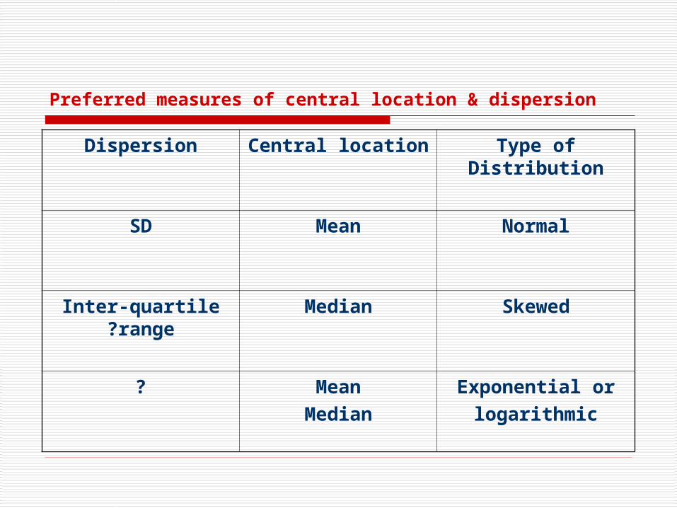
Preferred measures of central location & dispersion
Type of DistributionCentral locationDispersion
NormalMeanSD
SkewedMedianInter-quartile range?
Exponential or
logarithmic
Mean
Median
?

NORMAL DISTRIBUTION

Bell-shaped: specific shape that can be defined as an equation
Symmetrical around the mid point, where the greatest frequency if scores occur
Asymptotes of the perfect curve never quite meet the horizontal axis
Normal distribution is an assumption of parametric testing
Frequency Distribution: the Normal Distribution

Frequency Distribution: Different Distribution shapes

Measure of Central Tendency
Mean
Median Mode
Mean
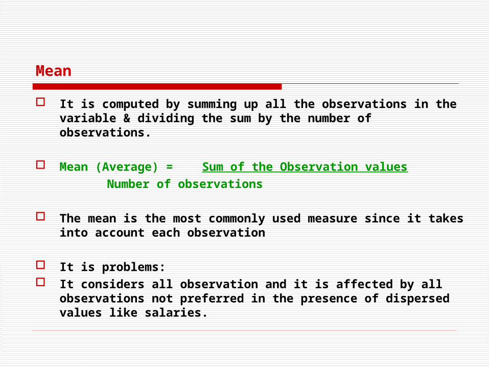
It is computed by summing up all the observations in the variable & dividing the sum by the number of observations.
Mean (Average) = Sum of the Observation values Number of observations
The mean is the most commonly used measure since it
takes into account each observation
It is problems: It considers all observation and it is affected by all
observations not preferred in the presence of dispersed values like salaries.
Mean (Average)
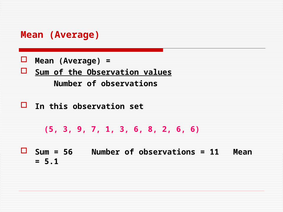
Mean (Average) = Sum of the Observation values
Number of observations
In this observation set
(5, 3, 9, 7, 1, 3, 6, 8, 2, 6, 6)
Sum = 56 Number of observations = 11 Mean = 5.1
Weighted Mean
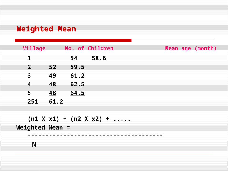
Village No. of Children Mean age (month)
1 54 58.6
2 52 59.53 49 61.24 48 62.55 48 64.5
251 61.2
(n1 X x1) + (n2 X x2) + .....Weighted Mean = --------------------------------------
N
Geometric Mean
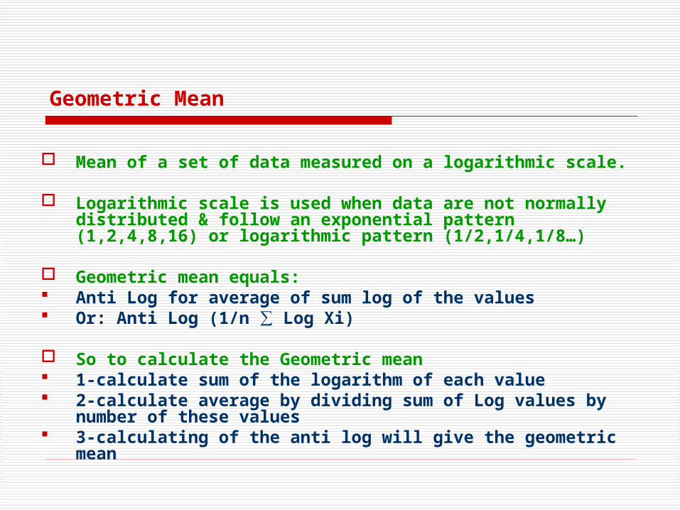
Mean of a set of data measured on a logarithmic scale.
Logarithmic scale is used when data are not normally distributed & follow an exponential pattern (1,2,4,8,16) or logarithmic pattern (1/2,1/4,1/8…)
Geometric mean equals: Anti Log for average of sum log of the values Or: Anti Log (1/n ∑ Log Xi)
So to calculate the Geometric mean 1-calculate sum of the logarithm of each value 2-calculate average by dividing sum of Log values by
number of these values 3-calculating of the anti log will give the geometric mean

Geometric Mean
Sample Dilution Titre
11:44
21:256256
31:22
41:1616
51:6464
61:3232
71:512512

Geometric Mean
Calculate the geometric mean:
1-Sum of Log (4, 256, 2, 16, 64, 32, 512) = 10.536
2. Average = 10.536 / 7 = 1.505
3- Anti Log average =32
Accordingly geometric mean =32
Geometric mean is important in statistical analysis of data following the previous described distribution such as sero survey where titer is calculated for different samples.

Median
Median: Value that divides a distribution into two equal parts.
Arrange the observation by order
1,2,3,3,5,6,6,6,7,8,9.
When the number is odd Median = No. + 1 = 11+1 = 6 2 2 So, median is the 6th observations = 6 The median is the best measure when the data is skewed
or there are some extreme values
Median
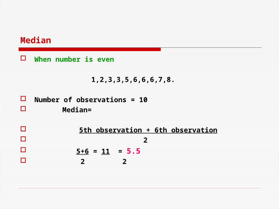
When number is even
1,2,3,3,5,6,6,6,7,8.
Number of observations = 10 Median=
5th observation + 6th observation 2 5+6 = 11 = 5.5 2 2
Mode
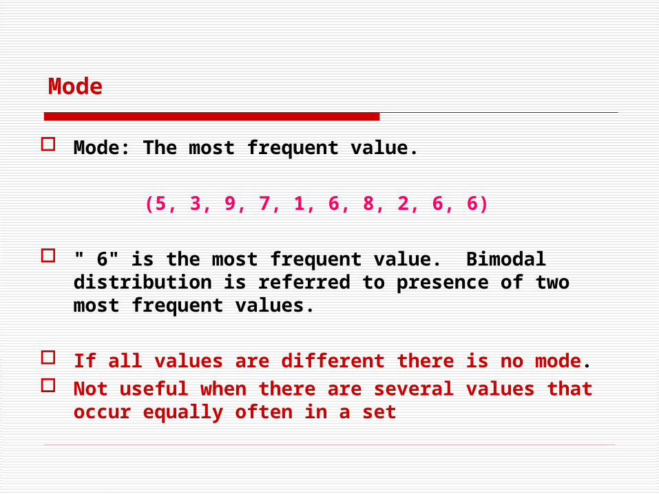
Mode: The most frequent value.
(5, 3, 9, 7, 1, 6, 8, 2, 6, 6)
" 6" is the most frequent value. Bimodal distribution is referred to presence of two most frequent values.
If all values are different there is no mode. Not useful when there are several values that
occur equally often in a set

Central Tendencies & Distribution Shape
The mean is > media when the curve is negatively skewed to left
The mean is < median when the curve is positively skewed to right
The mean, median and mode are equal when distribution is symmetrical. The mean is equal to median when it is symmetrical

Measures of Dispersion (Variation) (Indicate spread of value)
The observations whether homogenous orheterogeneous, the variability of the observations
1. Range2. Variance3. Standard deviation4. Coefficient of variation5. Standard error6. Percentiles & quartiles
Describing Variability: the Range
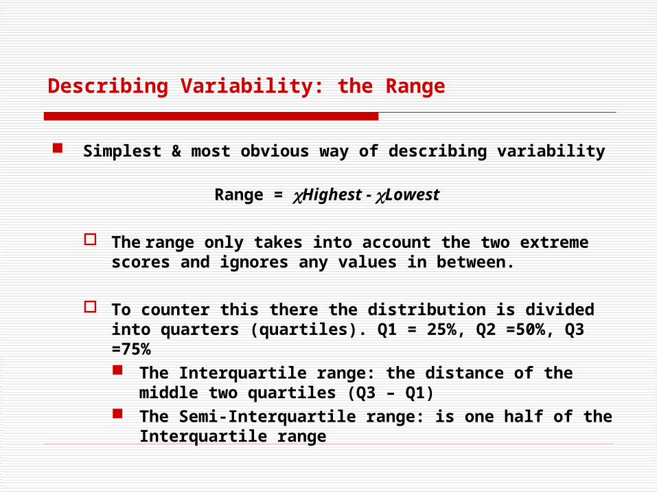
Simplest & most obvious way of describing variability
Range = Highest - Lowest
The range only takes into account the two extreme scores and ignores any values in between.
To counter this there the distribution is divided into
quarters (quartiles). Q1 = 25%, Q2 =50%, Q3 =75% The Interquartile range: the distance of the middle
two quartiles (Q3 – Q1) The Semi-Interquartile range: is one half of the
Interquartile range

Measures of Dispersion (Variation) (Indicate spread of value)
The observations whether homogenous or heterogeneous, the variability of the observations
1. Range The range is the difference between the largest
and the smallest observations. Range = maximum – minimum
Disadvantage: it depends only on two values & doesn’t take into account other observations

Measures of Dispersion (Variation) (Indicate spread of value)
2. Variance
It measures the spread of the observations around the mean.
If the observations are close to their mean, the variance is small, otherwise the variance is large.
Variance = S2 =
2
1
)(
n
xxi

Describing Variability: Deviation
A more sophisticated measure of variability is one that shows how scores cluster around the mean Deviation is the distance of a score from the mean
X - , e.g. 11 - 6.35 = 3.65, 3 – 6.35 = -3.35
A measure representative of the variability of all the scores would be the mean of the deviation scores(X - ) Add all the deviations and divide by n n However the deviation scores add up to zero (as
mean serves as balance point for scores)

Describing Variability: Variance
To remove the +/- signs we simply square each deviation before finding the average. This is called the Variance:
(X - )² = 106.55 = 5.33n 20
The numerator is referred to as the Sum of Squares (SS): as it refers to the sum of the squared deviations around the mean value

Describing Variability: Population Variance
Population variance is designated by ² ² = (X - )² = SS N N
Sample Variance is designated by s² Samples are less variable than populations: they
therefore give biased estimates of population variability
Degrees of Freedom (df): the number of independent (free to vary) scores. In a sample, the sample mean must be known before the variance can be calculated, therefore the final score is dependent on earlier scores: df = n -1 s² = (X - M)² = SS = 106.55 = 5.61
n - 1 n -1 20 -1

Describing Variability: the Standard Deviation
Variance is a measure based on squared distances In order to get around this, we can take the square root of
the variance, which gives us the standard deviation Population () & Sample (s) standard deviation
= (X - )² N
s = (X - M)² n - 1 So for our memory score
example we simple take the square root of the variance:
=5.61 = 2.37

Measures of Dispersion (Variation)
3. Standard deviation (SD)
It is the square root of the variance S = Both variance & SD are measures of variation in a set of data. The larger they are the more heterogeneous the distribution. SD is more preferred than other measures of variation.
Usually about 70% of the observations lie within one SD of their mean and about 95% lie within two SD of the mean
If we add or subtract a constant from all observations, the changed by the same constant, but the SD does not change
If we multiply or divide all the observation by the same constant, both mean & SD changed by the same amount
Small SD, the bell is tall & narrow Large SD, the bell is short & broad

Standard Deviation (SD)Example: Calculate SD for this observation set: (7,3,4,6)
Value Xi
Deviation from mean(Xi – X)
(Deviation)2
(Xi – X)2
724
3-24
4-11
611
20010
Mean (X) = 20 = 5 Mean of (Dev.)2 = 10 = 2.5 4 4
SD = = 1.6 5.2
Measures of Dispersion (Variation)
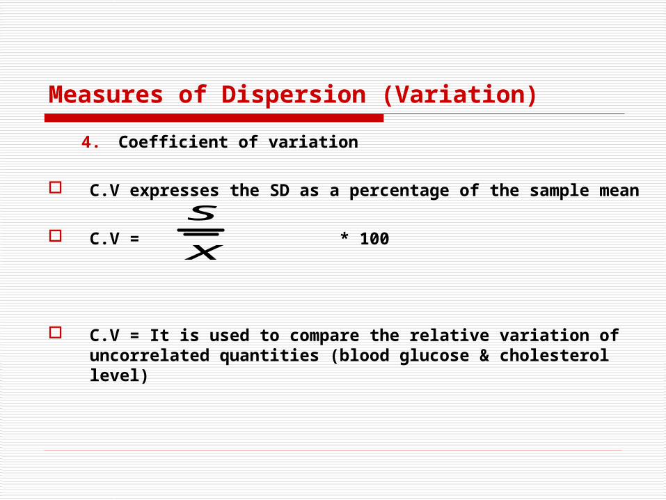
4. Coefficient of variation
C.V expresses the SD as a percentage of the sample mean
C.V = * 100
C.V = It is used to compare the relative variation of uncorrelated quantities (blood glucose & cholesterol level)
x
s

Measures of Dispersion (Variation)
5. Standard error SE measures how precisely the pp mean is estimated by
sample mean. The size of SE depends both on how much variation there is in the pp and on the size of the sample.
SE =
SE = If the SE is large, sample is not precise to estimate the pp.
n
s

Describing Variability
Describes in an exact quantitative measure, how spread out/clustered together the scores are
Variability is usually defined in terms of distance How far apart scores are from each other How far apart scores are from the mean How representative a score is of the data set as a
whole

Quartiles & Interquartiles
252830303233343536374040414244454555
The age range of this group of 18 students is 55 – 25 = 30 years
If the older student was not present, the range would have been 45 – 25 = 20 years
This means that a single value could give non-real wide range of the groups age
Since we can not ignore a single value and we do not want to give wrong impression, we estimate the interquartile range

Quartiles & Interquartiles
123456789101112131415161718
252830303233343536374040414244454555
First quartiles Second quartile
Third quartile Fourth quartile
Interquartile range
The values are arranged in ascending manner The groups then divided into 4 equal parts, each part contain one quarter of observations In the below example, 18/4 = 4.5 individuals The value of the fifth individual is the minimum value of the interquartile range As a general rule, when the product of division contains a fraction then take the following individual’s value (4.5, take the value of the fifth) Interquartile range = 42 – 32 = 10 years

Percentiles
Used when the number of observations is large
The values are arranged in ascending manner When the individuals are hundred, the lowest value
will be 1st percentile and the highest will be the 100th percentiles.


