Measures of Dispersion

RangeQuartile, interquartile range, semi-interquartile rangeVarianceStandard deviation

Range Range = Largest observation – smallest observation

For example, In U6A, the highest mark for Maths is 82 while the lowest is 26. The range is 56. In U6B, the highest mark for Maths is 75 while the lowest is 38. The range is 37.

Quartile Quartiles are values which divide a set of data

arranged in ascending or descending order into four equal parts.

The first quartile Q1, or the lower quartile – ¼ of the total number of data has values less than Q1.

The second quartile is the median.

The third quartile Q3, or the upper quartile – ¾ of the total number of data has values less than Q3.

Quartile, Interquartile & Semi-interquartile range for ungrouped data To find quartile, arrange the data in

ascending order, as in the following example: 23, 47, 32, 34, 42, 35, 44, 36, 52, 40, 42, 46

We also have: Interquartile range = Q3 – Q1

Semi-interquartile range = ½(Q3 – Q1)

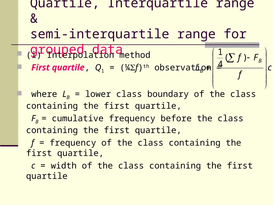
Quartile, Interquartile range &semi-interquartile range for grouped data

(i) Interpolation method First quartile, Q1 = (¼f)th observation =

where LB = lower class boundary of the class containing the first quartile, FB = cumulative frequency before the class containing the first quartile, f = frequency of the class containing the first quartile, c = width of the class containing the first quartile

cf

FfL

B

B

)(41

Quartile, Interquartile range &semi-interquartile range for grouped data

(i) Interpolation method Third quartile, Q3 = (¾f)th observation=

where LB = lower class boundary of the class containing the third quartile, FB = cumulative frequency before the class containing the third quartile, f = frequency of the class containing the third quartile, c = width of the class containing the third quartile

cf

FfL

B

B

)(43

Quartile, percentile

Beside quartile, we can also talk about percentile.

For example we can talk about the 15th percentile.

Variance Consider the data: 3, 4, 5, 6, 7. Mean = (3 + 4 + 5 + 6 + 7)/5 = 5

We wish to study how are the data deviate from the mean. So we find (xi - ) for each of the data.

Unfortunately, is always zero for any set of data.

To overcome this problem, we use the squares of these value.

The result: variance,

x

x

)( xxi

nxx

s i

22 )(

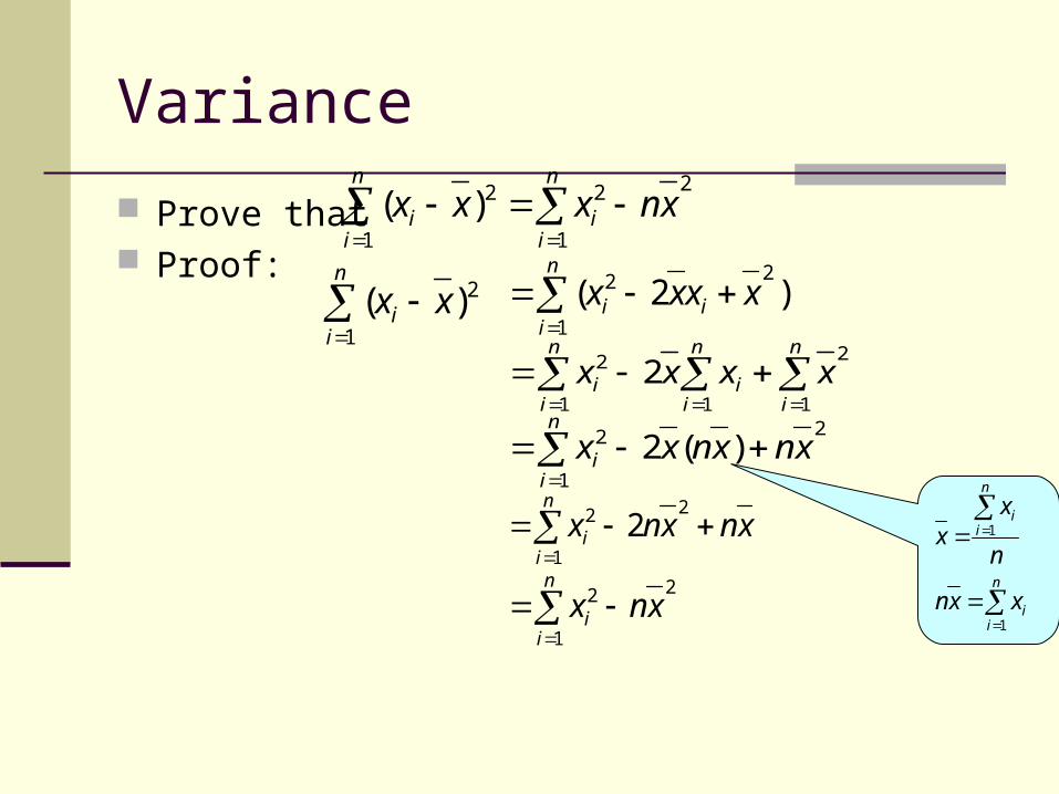
Variance Prove that Proof:

2

1

22

1)( xnxxx

n

ii

n

ii

2

1)(

n

ii xx

n

iii xxxx

1

22 )2(

n

i

n

ii

n

ii xxxx

1

2

11

2 22

1

2 )(2 xnxnxxn

ii

xnxnxn

ii

2

1

2 2

2

1

2 xnxn

ii

n

ii

n

ii

xxn

n

xx

1

1

Variance for ungrouped data For ungrouped data, the variance:

n

xxs

n

ii

1

2

2)(

21

2

2 xn

xs

n

ii

2

11

2

2

n

x

n

xs

n

i

n

ii

Variance for grouped data

For grouped data, the mid-point of each class, xi, is used to represent the class.

So, the variance is given by:

fxxf

s i2

2 )(

22

2 xffxs i

222

ffx

ffx

s i

Prove this.

Standard Deviation

In the process of finding variance, we have squared the data. This means that variance is one dimension more than the data.

For example, unit for the data: cm; unit for variance: cm2.

So variance is not a very useful measure. Instead, we take its square root and call it

standard deviation.

Standard Deviation for ungrouped data

For ungrouped data, the standard deviation is:

n

xxs

n

ii

1

2)(

21

2

xn

xs

n

ii

2

11

2

n

x

n

xs

n

i

n

ii

Standard Deviation for grouped data

For grouped data, the standard deviation is:

fxxf

s i2)(

22

xffx

s i

22

ffx

ffxs i

Standard deviation & variance by coding method Similar to the coding method for calculating mean.

hkxy

where k is the assumed mean,and h is the scaling factor.

Standard deviation of y:

fyyf

sy

2)(

fhkx

hkxf

sy

2

2

f

xxfhsy

2

22

1

22

2 1xy s

hs

yx hss

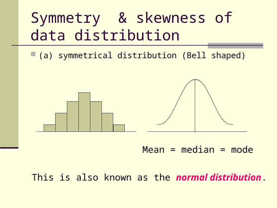
Symmetry & skewness of data distribution (a) symmetrical distribution (Bell shaped)

Mean = median = mode

This is also known as the normal distribution.

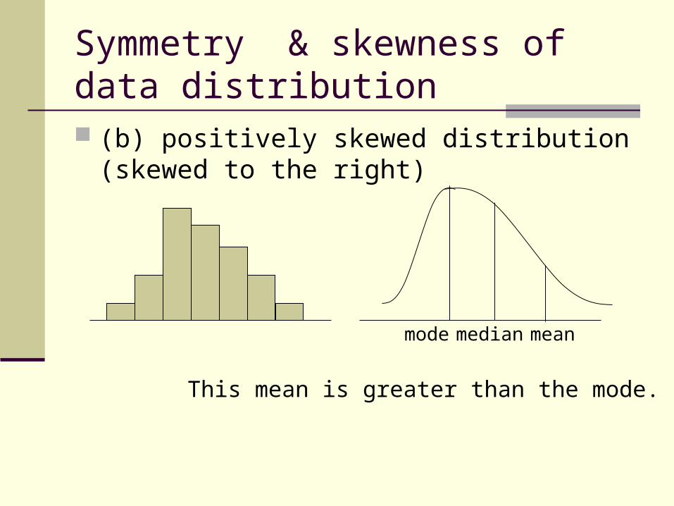
Symmetry & skewness of data distribution (b) positively skewed distribution (skewed to

the right)

This mean is greater than the mode.

mode median mean

Symmetry & skewness of data distribution (c) negatively skewed distribution (skewed to

the left)

This mean is less than the mode.

modemedianmean

Box-and-whisker plots (Boxplots)

This is another graphical representation of data.

(a) Horizontal box-and-whisker plot:

Lowest value Highest valueLower quartile Q1

Upper quartile Q3

Median Q2

(b) Vertical box-and-whisker plot

Box-and-whisker plots (Boxplots)

Lowest value

Lower quartile Q1

Median Q2

Upper quartile Q3

Highest value

The box extends from Q1 to Q3 andencloses the middle 50% of the data.

The whiskers extend from the box tothe lowest and highest values andillustrate the range of the data.

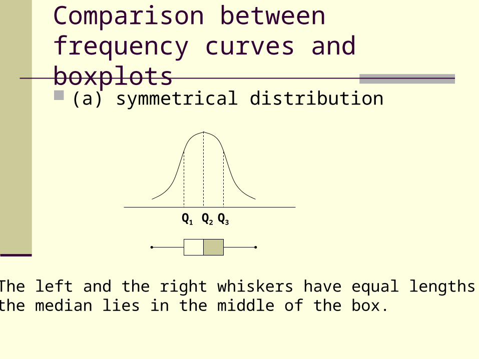
Comparison between frequency curves and boxplots (a) symmetrical distribution

Q1 Q2 Q3

The left and the right whiskers have equal lengths andthe median lies in the middle of the box.

Comparison between frequency curves and boxplots (b) positively skewed distribution

The left whisker is shorter than the right whisker andthe median lies closer to the lower quartile.

Q1 Q2 Q3

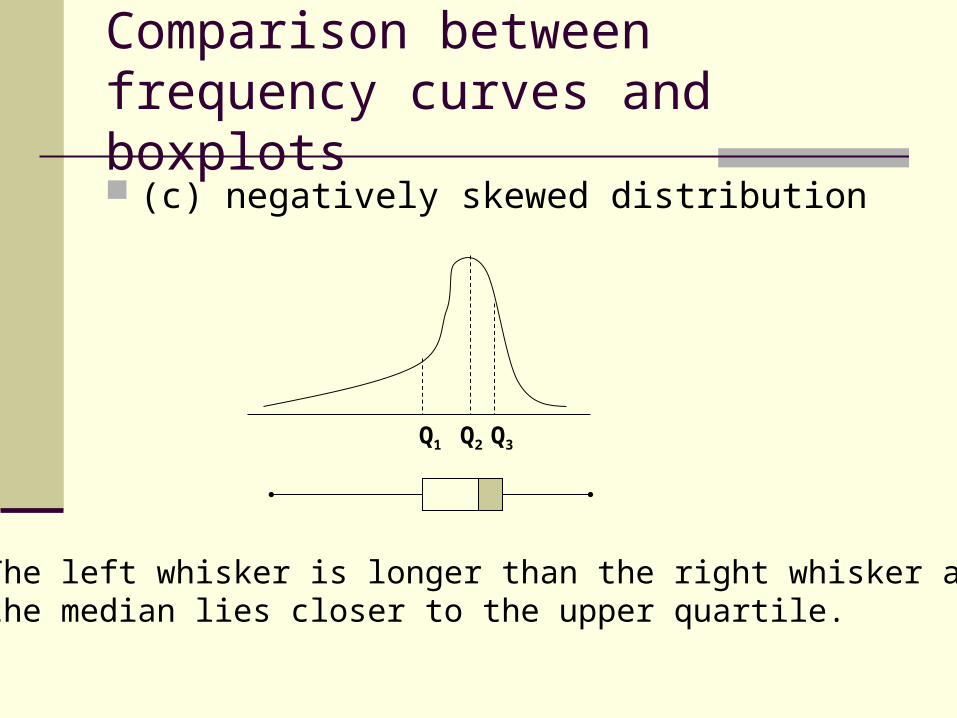
Comparison between frequency curves and boxplots (c) negatively skewed distribution

The left whisker is longer than the right whisker andthe median lies closer to the upper quartile.

Q1 Q2 Q3

Example of boxplot The stem-and leaf plot below shows the number of flies

caught in an insect trap for 28 days. 0 1 1 2 1 2 3 5 5 5 6 2 2 2 3 5 8 8 3 4 4 4 4 5 7 7 8 4 2 6 7 7 8 key: 1 | 2 means 12 flies (a) Illustrate the data by drawing a boxplot. (b) Use your boxplot to comment on the type of distribution.

Example of boxplot (a) From the data in the stemplot, the lowest

value is 1, the lower quartile = 15, the median = 28, the upper quartile = 37, and the highest value = 48.

(b) The left whisker is longer than the right whisker & the median lies closer to the upper quartile. Therefore, the distribution is negatively skewed.

0 10 20 30 40 50

1 15 28 37 48

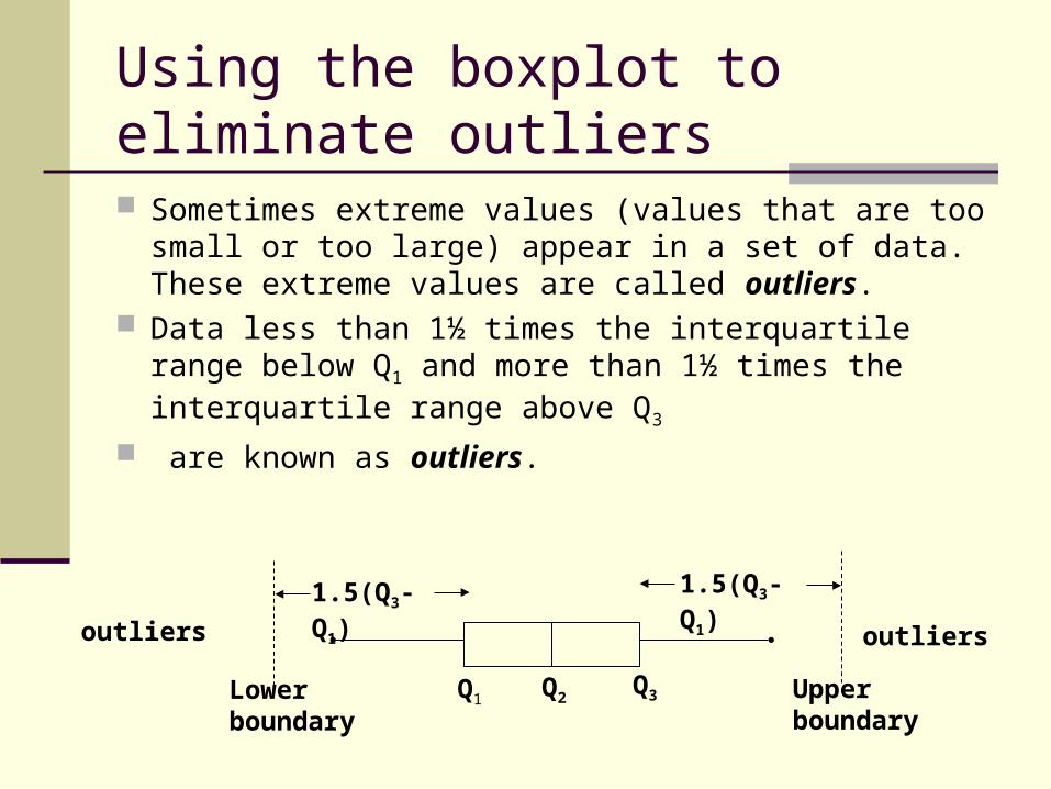
Using the boxplot to eliminate outliers

Sometimes extreme values (values that are too small or too large) appear in a set of data. These extreme values are called outliers.

Data less than 1½ times the interquartile range below Q1 and more than 1½ times the interquartile range above Q3

are known as outliers.

Q1 Q2 Q3

1.5(Q3-Q1) 1.5(Q3-Q1)

Lowerboundary

Upperboundary

outliers outliers

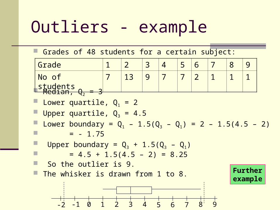
Outliers - example Grades of 48 students for a certain subject:

Median, Q2 = 3 Lower quartile, Q1 = 2 Upper quartile, Q3 = 4.5 Lower boundary = Q1 – 1.5(Q3 – Q1) = 2 – 1.5(4.5 – 2) = - 1.75 Upper boundary = Q3 + 1.5(Q3 – Q1) = 4.5 + 1.5(4.5 – 2) = 8.25 So the outlier is 9. The whisker is drawn from 1 to 8.

Grade 1 2 3 4 5 6 7 8 9No of students 7 13 9 7 7 2 1 1 1

-2 -1 0 1 2 3 4 5 6 7 8 9

Furtherexample