Measures of Price Sensitivity 1 - Faculty &...

9Measures of Price

Sensitivity 1

This chapter reviews the factors that cause bond prices to be volatile. TheMacaulay measure of duration and modified duration are described. This lat-ter measure captures the exposure of a bond to interest rate rmoves of a certainkind. Immunization strategies based on duration matching and duration-convexity matching are presented. The limitations of these approaches arediscussed. Measures of risk due to a twisting term structure are investigated.The basic measures of duration, convexity and twist risk are helpful in char-acterizing risk exposures.

For most of this chapter we assume the initial yield curve is flat. That is,the yields to maturity are the same for all maturities. We also assume thatwhen unanticipated information arrives causing the yield curve to change, thechange is the same for all maturities. Hence yield curves remain flat, and justmove up and down, depending on information. While this assumption is veryunrealistic it provides a start for our analysis. Later on in this chapter we willallow the initial yield curve to be arbitrary, but we will assume that all shocksto the yield curve are the same. In this case the yield curve never changes itsbasic shape, although it again moves up and down as information arrives. Ifnon parallel shocks, such as twists occur, then our measures of risk need to bereassessed. In future chapters we will consider alternative risk measures thatcan handle alternative types of shocks to the yield curve.

The purpose of this chapter is

161

162 CHAPTER 8: MEASURES OF PRICE SENSITIVITY 1

• To describe measures of duration and convexity in regard to bond pricevolatility,

• To discuss the use of duration and convexity measures in imunizationstrategies,

• To discuss other measures of interest rate sensitivity, including the dollarvalue of a basis point shock, and

• To provide the first step in establishing a framework for interest raterisk management.

9.1 PRICE-YIELD RELATIONSHIPS

Changes in the yield curve tend to affect the price of some fixed-income secu-rities more than others. The sensitivity of bond prices to interest rate changedepends on many factors, including current yields and yield chages, time tomaturity, and coupon size.

Effect of Yield Change

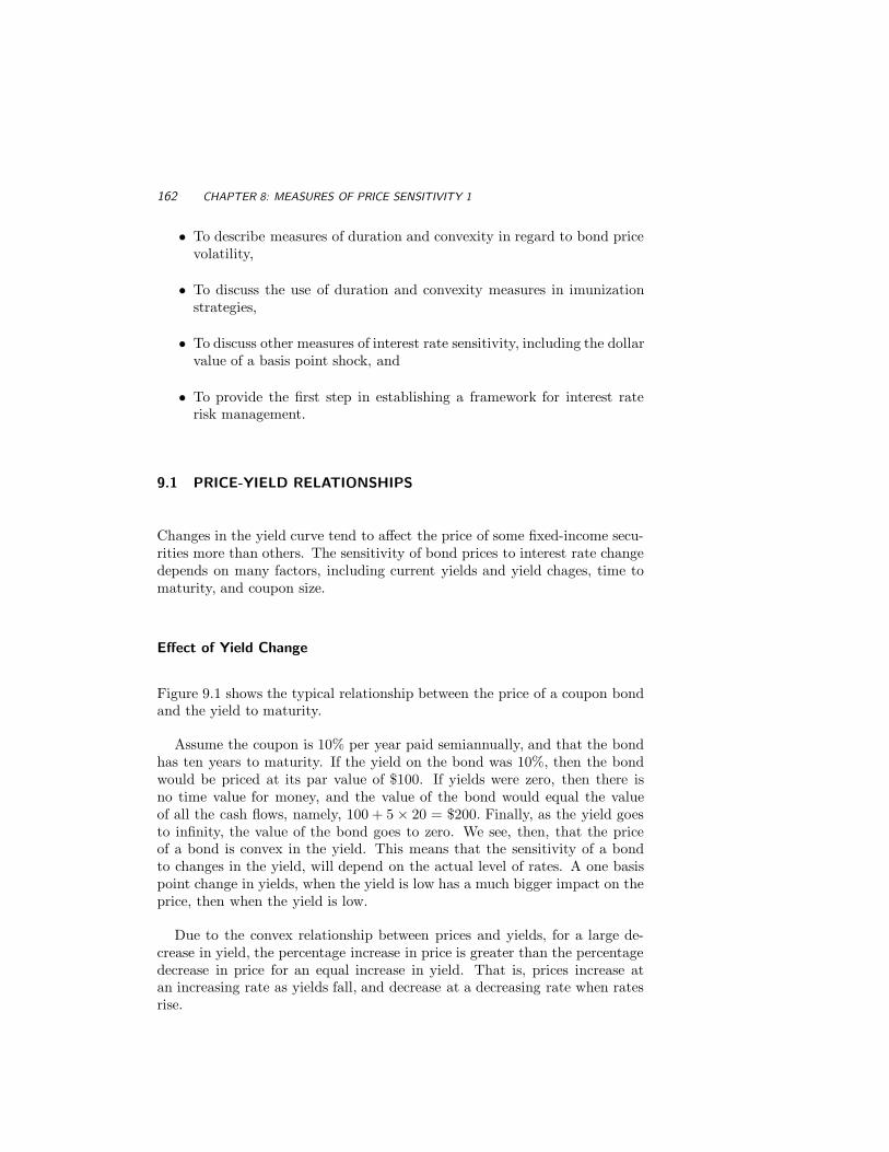
Figure 9.1 shows the typical relationship between the price of a coupon bondand the yield to maturity.

Assume the coupon is 10% per year paid semiannually, and that the bondhas ten years to maturity. If the yield on the bond was 10%, then the bondwould be priced at its par value of $100. If yields were zero, then there isno time value for money, and the value of the bond would equal the valueof all the cash flows, namely, 100 + 5 × 20 = $200. Finally, as the yield goesto infinity, the value of the bond goes to zero. We see, then, that the priceof a bond is convex in the yield. This means that the sensitivity of a bondto changes in the yield, will depend on the actual level of rates. A one basispoint change in yields, when the yield is low has a much bigger impact on theprice, then when the yield is low.

Due to the convex relationship between prices and yields, for a large de-crease in yield, the percentage increase in price is greater than the percentagedecrease in price for an equal increase in yield. That is, prices increase atan increasing rate as yields fall, and decrease at a decreasing rate when ratesrise.

PRICE-YIELD RELATIONSHIPS 163

Fig. 9.1 Price vs Yield on a Coupon Bond

Example

Consider a four-year 8% bond with annual coupons sold at par ($1000) toyield 8%. If yields fall to 6%, the bond price is

B =80

1.06+

801.062

+80

1.063+

10801.064

= $1069.30.

This yield change causes a 6.93% change in the bond price. If interest ratesrise to 10%, the bond price is

B =80

1.10+

801.102

+80

1.103+

10801.104

= $936.60.

This yield change causes a 6.34% change in bond price. Thus, a decreasein yields causes a larger percentage change in the price than an equivalentincrease in yields.


Effect of Maturity on Bond Prices

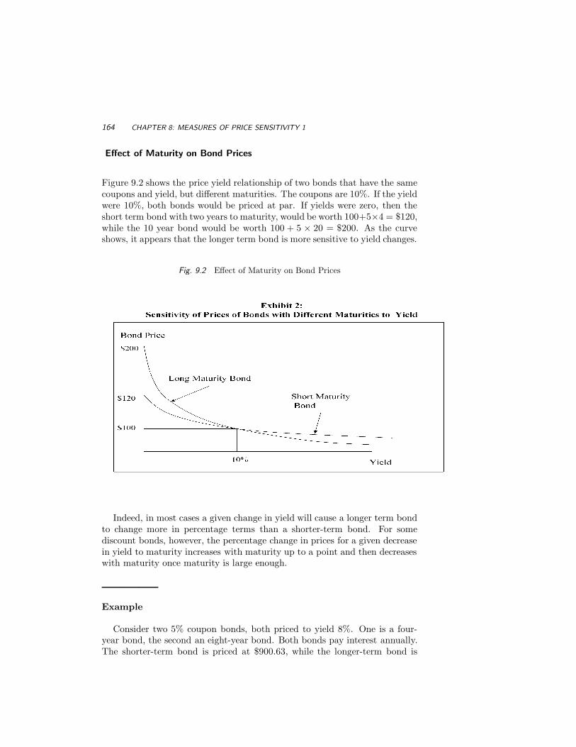
Figure 9.2 shows the price yield relationship of two bonds that have the samecoupons and yield, but different maturities. The coupons are 10%. If the yieldwere 10%, both bonds would be priced at par. If yields were zero, then theshort term bond with two years to maturity, would be worth 100+5×4 = $120,while the 10 year bond would be worth 100 + 5 × 20 = $200. As the curveshows, it appears that the longer term bond is more sensitive to yield changes.

Fig. 9.2 Effect of Maturity on Bond Prices

Indeed, in most cases a given change in yield will cause a longer term bondto change more in percentage terms than a shorter-term bond. For somediscount bonds, however, the percentage change in prices for a given decreasein yield to maturity increases with maturity up to a point and then decreaseswith maturity once maturity is large enough.

Example

Consider two 5% coupon bonds, both priced to yield 8%. One is a four-year bond, the second an eight-year bond. Both bonds pay interest annually.The shorter-term bond is priced at $900.63, while the longer-term bond is

PRICE-YIELD RELATIONSHIPS 165

priced at $827.60. Assume yields rise to 10%. Then, from the bond pricingequation, the four-year bond will be priced at $841.50, while the eight-yearbond will be priced at $733.40. In percentage terms, the decline in price ofthe shorter-term bond is 6.6%, compared to 11.4% for the longer-term bond.

Effect of Coupon Size on Bond Prices

Figure 9.3 compares the the price yield relationship for a 10 year bond thathas coupons of 14% per year with that of an otherwise identical bond with acoupon of 10%. If the yield was 14%, then the first bond would be priced atpar. Moreover, if the yield were zero, then the price would be 100 + 7× 20 =$240.

Fig. 9.3 Effect of Coupons on Price

Since this bond has all the features of the lower coupon bond, except thatit pays out more, it has to be the case that its price yield curve lies abovethe curve of the lower coupon bond. Which of the above two bonds has thegreater risk? Put another way, given a change in yields, which bond willchange more in percentage terms?


A given change in yields will cause the price of the lower-coupon bond tochange more in percentage terms. The reason for this follows from the factthat higher-coupon bonds, having greater cash flows, return a higher propor-tion of value earlier than lower-coupon bonds. This implies that relativelyless of the high-coupon bond faces the higher compounding associated withthe new discount factor. Therefore, on a relative basis, less price adjustmentis required for the higher-coupon bond.

Example

Consider two four-year annual coupon bonds, both priced to yield 8%.The first bond has a 5% coupon, the second a 10%. From the bond pricingequation, their prices are $900.63 and $1066.24, respectively. Assume interestrates change so that each bond is now priced to yield 10%. Then the newbond prices are

B1 =50

1.10+

501.102

+50

1.103+

10501.104

= $841.50

B2 =1001.10

+100

1.102+

1001.103

+11001.104

= $1000

In percentage terms, the 5% coupon bond has changed by (900.63−841.50)/900.63) =6.6% while the 10% coupon bond has changed by 6.2%. In general, low-couponbonds are more sensitive to yield changes than high-coupon bonds.

Bonds trading above their face value (premium bonds) have higher couponrates than bonds trading below their face value (discount bonds) and, hence,all things being equal, will be less sensitive to yield changes.

In summary, the price sensitivity of a coupon bond is affected by its couponrate and maturity as well as the current level of yield. In general, for a givenmaturity, the lower the coupon rate the greater the volatility, and for a fixedcoupon, the greater the maturity the greater the volatility. To compare therisk of bonds with different coupons and different maturities a measure calledduration is required. This is considered next.

9.2 MACAULAY DURATION

Since high coupon bonds provide a larger proportion of total cash flow earlierin the bond’s life than lower coupon bonds with the same maturity, they are

CHAPTER 8: MACAULAY DURATION 167

effectively shorter term instruments. As a result, the actual maturity date ofthe bond is not necessarily a good measure of the length of a coupon bond.

To obtain a more meaningful measure it is helpful to first represent thebond as a portfolio of discount bonds and to measure the maturity of eachcash flow. From the bond pricing equation:

B0 =m∑

t=1

P (0, t)CFt.

Let wt be the present value contribution of the tth cash flow to the bondprice. Then

wt =P (0, t)CFt

B0for t = 1, 2, ...., m

The duration, D, of a bond is just the weighted average number of periods forcash flows for this bond. That is

D =m∑

t=1

t × wt

Notice that the greater the time until payments are received, the greaterthe duration. If the bond is a discount bond, all payment is deferred tomaturity and the duration equals maturity. For bonds making periodic couponpayments the early payments will reduce the duration away from the maturity.

Macaulay Duration is affected by changes in the market yield, the couponrate and the time to maturity.

Example

Consider a 4-year bond paying a 9% coupon semi-annually and priced toyield 9%. The cash flows every 6 months are shown below, as well as theweights and duration calculation.


Period Cash Flow Present Value Weighted Present Valuet CFt P (0, t)CFt tP (0, t)CFt

1 45 43.06 43.062 45 41.21 82.423 45 39.43 118.34 45 37.74 150.945 45 36.11 180.556 45 34.56 207.337 45 33.07 231.476 1045 734.83 5878.63

Total 1000.0 6892.70

The duration is 6892.70/1000 = 6.89 half years, or 3.45 years.

Example

The sensitivities of durations to changes in yield, coupons, and maturityfor a five-year bond that pays 12% annual coupons and yields 12% percentare shown below.

• All factors being equal, the higher the yield, the lower the duration.

Yield 4 8 12 16 20

Duration 4.2 4.1 4.0 3.7 2.9

• All factors being equal, the higher the coupon, the lower the duration.

Coupon 4 8 12 16 20

Duration 4.5 4.2 4.0 3.9 3.8

• For this bond the duration increases with maturity. This property istypical, but may not always hold. The exception to this rule will be lowcoupon bonds with long maturity.

Maturity 3 5 7 10 30

Duration 2.7 4.0 5.1 6.3 9.0

CHAPTER 8: DURATION AND BOND PRICE SENSITIVITY 169

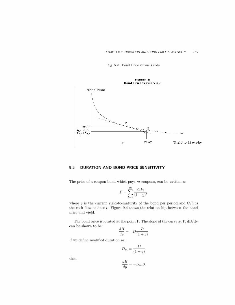
Fig. 9.4 Bond Price versus Yields

9.3 DURATION AND BOND PRICE SENSITIVITY

The price of a coupon bond which pays m coupons, can be written as

B =m∑

t=1

CFt

(1 + y)t

where y is the current yield-to-maturity of the bond per period and CFt isthe cash flow at date t. Figure 9.4 shows the relationship between the bondprice and yield.

The bond price is located at the point P. The slope of the curve at P, dB/dycan be shown to be:

dB

dy= −D

B

(1 + y)

If we define modified duration as:

Dm =D

(1 + y)

thendB

dy= −DmB


ordB

B= −Dmdy

That is, the instantaneous percentage change in bond price equals the negativeof modified duration times the change in yield, provided the change in yieldis very small.

If a bond has a modified duration of 4.0 then its market value will changeby 4% when the yield per period changes by 1% or equivalently by 100 basispoints. The higher the modified duration the more exposed the bond is tointerest rate changes.

Example

Consider the previous 4-year bond paying a 9% coupon semi-annually andpriced to yield 9% per year, or 4.5% per six-month period. The duration ofthe bond is 6.89 periods. The modified duration is therefore

Dm = D/(1 + y) = 6.89/1.045 = 6.593 periods or 3.297 years.

For a one percentage change in the annual yield to maturity, the percentagechange in the bond price is 3.297%.

9.4 DURATION OF A BOND WITH UNEVEN PAYMENTS

In our analysis we have assumed that the compounding interval equals thetime between successive cash flows. In particular, y is the rate per period. Inmost cases, coupon payments are equally spaced, except for the first couponpayment. Let p be the fraction of a period till the first coupon date. Forexample if the time between coupon dates is 6 months, and the time to thefirst coupon date is 2 months, then with each period corresponding to a sixmonth interval, p = 2/6. The Macaulay duration is:

D =m∑

t=1

(p + t − 1)wt

wherewt =

CFt

(1 + y)p+tB(0)

CHAPTER 8: APPROXIMATIONS FOR THE CHANGE IN A BOND PRICE 171

is the relative contribution to the bond price made by the present value of thetth cash flow. It can be shown that the modified duration is given by

Dm = D∗m − (1 − p)

where D∗m is the modified duration of the same bond computed with p=1.

Example

To be done

9.5 LINEAR AND QUADRATIC APPROXIMATIONS FOR THE

CHANGE IN A BOND PRICE

Assume the yield changes from y to y + ∆y, where ∆y is small. The bondprice in Exhibit 4 then changes from B(y) (point P) to B(y + ∆y) (point Q).For ∆y sufficiently small, B(y + ∆y) can be approximated by B′(y + ∆y)where

B′(y + ∆y) ≈ B(y) +dB

dy∆y

which is indicated by point S in the above diagram. Since dB/dy = −DmB,the above equation can be rewritten as

B′(y + ∆y) ≈ B(y) − DmB(y)∆y

Note that if ∆y is “large” positive or negative, then the linear, or first orderapproximation, B′(y + ∆y), is always lower than the actual bond price. Theerror is attributable to the curvilinear or convex relationship between bondprices and yields.

To account for this convexity, we could use a second order approximation,which takes into consideration how the slope changes as the yield y changes.For convex relationships, the change in the slope is always increasing. Forexample, the slope at the point Q is less negative than the slope at pointP. A second order approximation of B(y + ∆y) which takes into account thecurvilinear relationship is given by

B′′(y + ∆y) ≈ B(y) +dB

dy∆y +

12

d2B

dy2(∆y)2


This can be rewritten as:

B′′(y + ∆y) ≈ B(y) − DmB(y)∆y +12C(y)B(y)(∆y)2

where

C(y) =d2Bdy2

B(y)

is defined as the convexity of the bond. In this case, differentiating the bondprice equation two times we obtain:1

C(y) =m∑

t=1

t(t + 1)CFt

(1 + y)t+2B(y)

The convexity of a straight coupon bond is always positive, implying thatthe slope of the price yield equation is increasing (becoming less negative) asyields increase.

The quadratic approximation differs from the linear approximation by thelast convexity term. Since this term is always positive, the quadratic approx-imation will always provide higher values than the linear approximation.

For small changes in the yield to maturity, the linear approximation pro-vides a good proxy for the change in bond price. That is, modified duration isa useful measure for price volatility. However, when the market perceives in-terest rate volatility to be high, then the second order approximation is moreprecise.

Example

Consider a 5 year bond which pays $80 in coupons semiannually (i.e., $40per 6 months), has a face value of $1000 and is currently priced to yield 8%per year. The duration of this bond is 8.435 periods (half years), and themodified duration is 8.435/1.04 = 8.111 periods. The convexity of the bondis 80.75 periods squared.

In this example, each period corresponds to a six month interval. To con-vert the convexity measure to an annual figure requires dividing by the square

1In this calculation, the assumption is made that the cash flows are equally spaced, that is,p = 0.

CHAPTER 8: APPROXIMATIONS FOR THE CHANGE IN A BOND PRICE 173

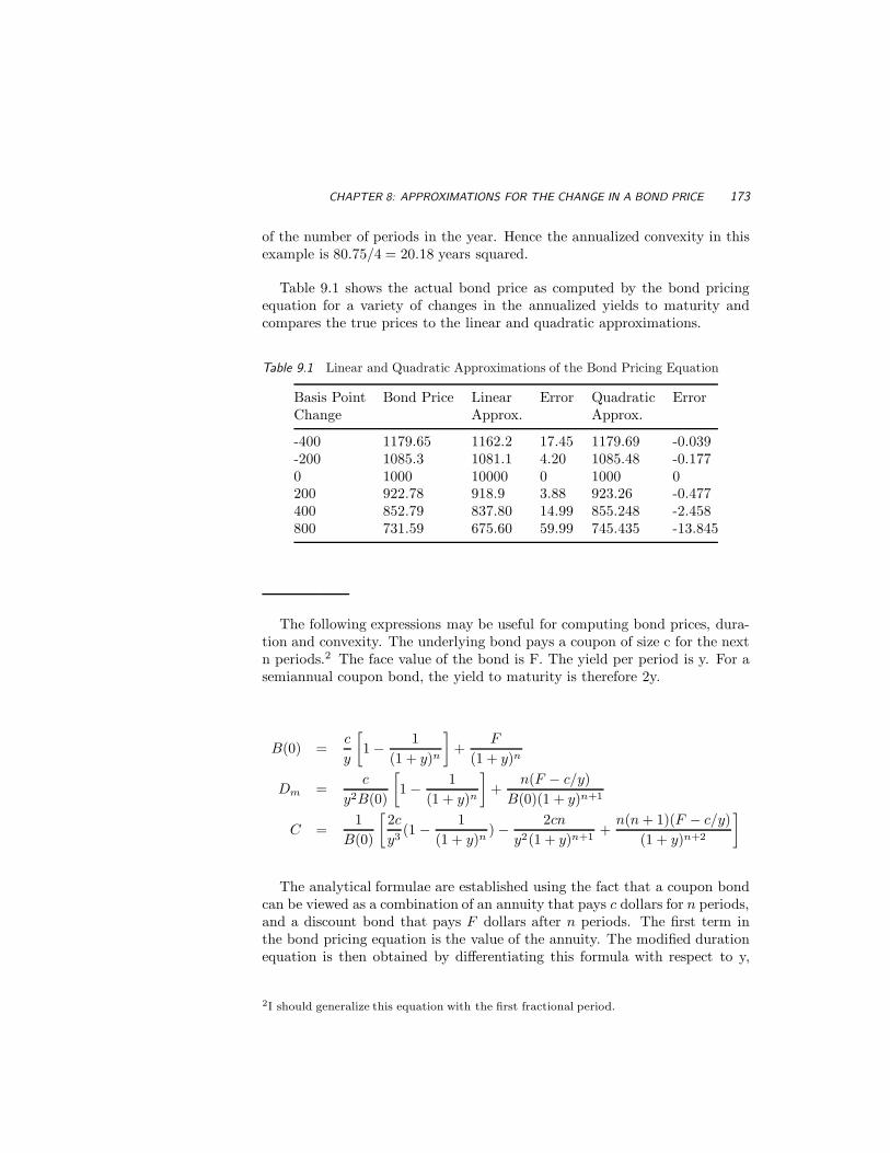
of the number of periods in the year. Hence the annualized convexity in thisexample is 80.75/4 = 20.18 years squared.

Table 9.1 shows the actual bond price as computed by the bond pricingequation for a variety of changes in the annualized yields to maturity andcompares the true prices to the linear and quadratic approximations.

Table 9.1 Linear and Quadratic Approximations of the Bond Pricing Equation

Basis Point Bond Price Linear Error Quadratic ErrorChange Approx. Approx.

-400 1179.65 1162.2 17.45 1179.69 -0.039-200 1085.3 1081.1 4.20 1085.48 -0.1770 1000 10000 0 1000 0200 922.78 918.9 3.88 923.26 -0.477400 852.79 837.80 14.99 855.248 -2.458800 731.59 675.60 59.99 745.435 -13.845

The following expressions may be useful for computing bond prices, dura-tion and convexity. The underlying bond pays a coupon of size c for the nextn periods.2 The face value of the bond is F. The yield per period is y. For asemiannual coupon bond, the yield to maturity is therefore 2y.

B(0) =c

y

[1 − 1

(1 + y)n

]+

F

(1 + y)n

Dm =c

y2B(0)

[1 − 1

(1 + y)n

]+

n(F − c/y)B(0)(1 + y)n+1

C =1

B(0)

[2c

y3(1 −

1(1 + y)n

) −2cn

y2(1 + y)n+1+

n(n + 1)(F − c/y)(1 + y)n+2

]

The analytical formulae are established using the fact that a coupon bondcan be viewed as a combination of an annuity that pays c dollars for n periods,and a discount bond that pays F dollars after n periods. The first term inthe bond pricing equation is the value of the annuity. The modified durationequation is then obtained by differentiating this formula with respect to y,

2I should generalize this equation with the first fractional period.


and dividing by the bond price. Similarly, the convexity equation is obtainedby differentiating this bond pricing equation twice with respect to y, and thendividing by the bond price.

9.6 PRICE VALUE OF A BASIS POINT

A very common risk measure is the sensitivity of the price of a bond to changesin its yield. The price value of a basis point, PV BP , sometimes called thedollar value of a basis point, or DV 01, measures the decline in price associatedwith a one basis point increase in the yield.

DV 01 = −Slope of Price Yield Curve × 0.01%

or

DV 01 = −dB

dy× 0.0001

DV01 can be computed directly, by computing the price at the current yield,adding one basis point to the yield, and recomputing the price.

Example

A five year bond pays 10% coupons semi annually and is priced at par. (y =0.10). To compute DV01 we reprice the bond at a yield of 0.1001. This leadsto a price of $99.9614. Hence, DV 01 = 100− 99.9614 = $0.0386.

DV01 can also be computed directly from modified duration. In particular,we have seen that

dB

B= −Dmdy

HencedB = −DmBdy

andDV 01 = −DmB × 0.0001

Example

CHAPTER 8: DURATION, CONVEXITY AND DV01 OF A BOND PORTFOLIO 175

Reconsider our five year bond that pays 10% coupons semi annually and ispriced at par. (y = 0.10). The modified duration of this bond is Dm = 3.86.Hence DV01 = 100× 3.86× 0.0001 = $0.0386.

9.7 DURATION, CONVEXITY AND DV01 OF A BOND PORTFOLIO

Like the beta value of an equity portfolio, the duration of a bond portfolio,Dp, is computed as the weighted average of the durations of the individualbonds:

Dp =K∑

i=1

αiDi

where K is the number of different bonds and αi is the fraction of portfoliodollars invested in bond i. Similarly, the convexity of a bond portfolio, Cp ,is the weighted average of the convexities of the individual bonds.

Cp =K∑

i=1

αiCi

The DV01 of a portfolio is defined as the change in value resulting fromequal one basis point declines in all yields. Let DV 01i represent the dollarvalue of a basis point associated with the ith bond. Then

DV 01p =K∑

i=1

xiDV 01i

where xi is the number of bonds of type i in the portfolio.

Example

A portfolio consists of 2 bonds. The first position is in three 5 year zero couponbonds, the second is in one 2 year zero coupon bond. The yield curve is flatat 10%, semiannually compounded. Durations of zero coupon bonds equaltheir maturities. The modified durations of the two bonds are 2

1.05= xxx

and 51.05 = yyy respectively. DV O11 = xxx × 0.0001 × 100

(1.05)10 = qqq andDV 012 = yyy × 0.0001× 100

(1.05)4 = rrr. Hence

DV 01p = 3qqq + 1rrr = $zzz


A one basis point increase will decrease the bond portfolio by $zzz.

9.8 HEDGING UNDER A PARALLEL SHIFT ASSUMPTION

Assume an investor holds a portfolio that has a DVO1 equal to DV 01p. As-sume that the investor wants to reduce the DV01 to zero. The resultingposition will then not change value for a small shock in the yield curve. Inorder to do this, we assume, at least for the moment that the yield curve shiftsup one basis point. That is, there is a parallel shock. Let DV 01h be the DV01value associated with the hedging instrument. For example, it could be a fiveyear coupon bond. The number of units required of the hedging instrumentis chosen such that

DV 01p + nhDV 01h = 0

ornh = −DV 01p

DV 01h

The negative sign indicates that a short position in the hedging contractsis necessary.

Example

Assume a position is held that has a DV01 of 500 dollars per million facevalue. Assume the hedging instrument consists of our 5 year coupon bondyielding 10%. Its DV01 is0.0386 per 100dollars. The number of 5 year bondsto trade is

nh = − 5000.0386

= −vvvv

By selling short vvv of the five year coupon bonds, the position is immunizedfrom a parallel shock of 1 basis point.

The above example assumes that a parallel shock of one basis point occursat all maturities. This implies that there is perfect correlation of changes inyields of the two securities. Later on we shall consider the case of hedgingwhen we allow for non parallel shocks in the yield curve.

CHAPTER 8: IMMUNIZATION OF INTEREST RATE RISK 177

9.9 IMMUNIZATION OF INTEREST RATE RISK

Consider an investor whose goals require that an investment be dedicated tomeet a specific liability of nominal amount F that comes due in m periods.If the investor held a portfolio of discount bonds having face value F andmaturity m, then, regardless of interest rate behavior, the future value of theportfolio would cover the future liability. This dedicated portfolio is said tobe perfectly immunized since its value is insensitive to changes in the yieldcurve.

Rather than use a discount bond, assume a coupon bond was held. Withcoupon bonds, two types of risk exist, price risk and coupon reinvestment risk.Price risk is the risk that the bond will be sold at a future point in time fora value different from what was expected. Coupon reinvestment risk is therisk associated with reinvesting the coupons at rates different from the yieldof the bond when it was purchased. If the maturity date coincides with theholding period, then price risk is eliminated. As the maturity date increases,so does price risk.

As interest rates increase (decrease), bond prices decline (increase) whilethe returns from reinvested coupon receipts increase (decrease). The fact thatprice risk and reinvestment risk move in opposite directions and are subjectto the same influences offers a way to manage interest rate risk. The choiceof the appropriate coupon and maturity bond to hold over a given investmentholding period is often accommodated by means of duration.

To illustrate the general idea consider the case where the yield curve is flatbut immediately after the bond is purchased the yield changes to some newvalue and stays there. In this case, the investor is faced with both reinvestmentand price risk, and after m periods, the liability may not be covered by theaccrued value of the coupons and the residual price of the bond. To focus onthis problem, assume the firm has a future obligation of $F to be paid out inm periods. The current value of the liability is V , where

V0(y) = F/(1 + y)m

To meet this obligation the firm reserves V0 dollars, and uses this cash topurchase a coupon bond with maturity n, say. The value of this bond is

V1(y) =n∑

i=1

CFi

(1 + y)i

Here, CFi is the cash flow of the bond in period i, and, since the yield curveis flat, the yield y in both equations are the same. Moreover, by construction,the number of bonds purchased is such that V0(y) = V1(y).


Now, assume a small shift in the yield curve occurs from y to y + ∆y. Thevalue of the liability changes from V0(y) to V0(y + ∆y), while the value of thebond changes from V1(y) to V1(y + ∆y). From the quadratic bond pricingapproximating equation we have:

V0(y + ∆y) ≈ V0(y) − D0mV0(y)∆y +

12C0V0(y)(∆y)2

V1(y + ∆y) ≈ V1(y) − D1mV1(y)∆y +

12C1V1(y)(∆y)2

For the liability to be immunized by the bond, their market values after theinterest rate change should remain equal. Since V0(y) = V1(y) this implies:

−D0mV0(y)∆y +

12C0V0(y)∆y)2 = −D1

mV1(y)∆y +12C1V1(y)∆y)2

For small interest rate changes the convexity adjustments are insignificantand the above equation reduces to

D0m = D1

m

That is the modified duration of the assets should be chosen to equal themodified duration of the liability.

In summary, we have shown that if the yield curve is flat, with a smallparallel shift occurring after purchase of the bond, then, for the market valueof the coupon bond to equal the market value of the future obligation, theduration of the bond selected should equal the holding period. Since, in ourexample the duration of the liability is m, the target bond portfolio shouldalso have a duration of m.

The above result is really only approximate since the convexity adjustmentswere ignored. If the change in yields are large, this approximation may nothold very well. If a tighter immunization is required then the convexitiesshould be matched as well. That is C0 = C1. For our particular problem,using the convexity equation, the convexity of the liability is given by

C0(y) =m(m + 1)F

(1 + y)2+mV0(y)

Substituting for V0(y) and simplifying leads to

C0(y) =m(m + 1)(1 + y)2

A bond having a modified duration of m, and satisfying the above equationwill more precisely match the liability than an alternative bond that merelymatches the duration.


Example

Consider a five-year bond that pays 12% annual coupons and yields 12%.Assume the investment horizon is four years. Since the modeified duration isfour years, the bond is locally immunized. If rates fall immediately to 11%and stayed there over the four-year period, the drop from coupon reinvestmentreturns would be offset exactly by increases in the price of the bond.

Example

A $1480 liability is due in 10 periods (5 years). The yield curve is currentlyflat at 4% per period (8% per year). With semiannual compounding thepresent value of this liability is V0(y) = 1480/(1.04)10 = $1000.

To immunize this liability an investor is considering purchasing the appro-priate number of units of a bond that pays $69.75 every period, has a facevalue of $1, 000, and matures in 14 periods. The current price of the bond is$1, 314.25, and its duration is 10 periods. Suppose $1, 000 (or 0.7609 units)of the bond were purchased. If the yield curve stays flat at 8%, and if allcoupons are reinvested, then the value of this portfolio after 5 years wouldequal the liability of $1480.

If, on the other hand, after buying the bond, the yield to maturity changedfrom 8 to 10 percent, and stayed there, then all bond prices would drop.However, the higher returns on coupon income would partially offset thisprice drop. The total accumulated value from holding one bond for 5 years(10 periods) is given by

10∑

i=1

CF (1.05)i +4∑

i=1

CF

(1.05)i+

1000(1.05)4

= $1947.34

where CF = $69.75 is the coupon payout in each period. Hence, the totalvalue of 0.7609 units of the bond is (0.7609)(1947.34) = $1481.7, which issufficient to meet the $1480.0 liability.

Figure 9.5 shows the accrued value of the portfolio for different changes inthe yield curve.

Notice that regardless of the shift in the yield curve, price risk is offset byreinvestment risk and the accrued value from the portfolio always exceeds theliability.

Table 9.2 shows information on two alternative bonds, bonds, A and C.


Fig. 9.5 Accrued Value of the Portfolio for Different Parallel Shocks

Table 9.2 Information on Two Bonds

Bond A Bond B Bond C

Bond Price 1219 1314 1407Amount of Bond 0.8203 0.7609 0.7103Semiannual Yield 4% 4% 4%Maturity (Periods) 10 14 20Coupon 67 69.75 70Face Value 1000 1000 1000Duration 7.85 10 12.71

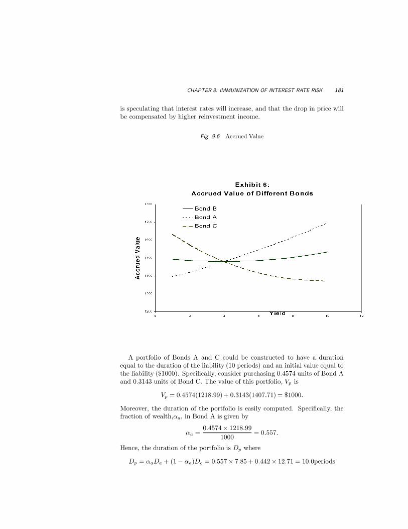
The previous analysis is repeated for these bonds and illustrated in Figure9.6.

Notice that the total accumulated value after 5 years may not be suffi-cient to meet the liability. For example, by holding bond C, the investor isspeculating that interest rates will decrease and that the loss of reinvestmentincome, obtained from lower yields will be more than offset by the accompa-nying price increase. Similarly, if Bond A (low duration) is held, the investor


is speculating that interest rates will increase, and that the drop in price willbe compensated by higher reinvestment income.

Fig. 9.6 Accrued Value

A portfolio of Bonds A and C could be constructed to have a durationequal to the duration of the liability (10 periods) and an initial value equal tothe liability ($1000). Specifically, consider purchasing 0.4574 units of Bond Aand 0.3143 units of Bond C. The value of this portfolio, Vp is

Vp = 0.4574(1218.99)+ 0.3143(1407.71) = $1000.

Moreover, the duration of the portfolio is easily computed. Specifically, thefraction of wealth,αa, in Bond A is given by

αa =0.4574× 1218.99

1000= 0.557.

Hence, the duration of the portfolio is Dp where

Dp = αaDa + (1 − αa)Dc = 0.557× 7.85 + 0.442× 12.71 = 10.0periods


Figure ?? compares the accrued value of this portfolio to the earlier bond,Bond B. The above analysis reveals that many portfolios of bonds could beconstructed to have the same duration as the targeted liability, and hence theportfolio that immunizes the liability by duration matching is not unique. Inthe above example the portfolio of bonds appears to be superior to Bond Bbecause the portfolio’s accrued terminal value is larger, for all yield shifts.

Fig. 9.7 Comparison of Accrued Values of Portfolio vs Bond B

Rather than match the convexity of the liability we might conclude thatamong all duration matched bond portfolios, the best portfolio is the one withthe highest convexity. The appropriate portfolio of bonds that achieves max-imum convexity can be obtained by solving the following linear programmingproblem.

Maximize∑K

i=1 αiCi

subject to∑K

i=1 αiDi = m∑K

i=1 αi = 1


where αi is the proportion of wealth allocated to bond i, and K representsthe number of candidate bonds. A duration matched bond portfolio havingmaximum convexity has the property that the selected bonds usually haveextreme durations and/or maturities. Such a portfolio is called a barbell port-folio since the pattern of cash flows reach their maximums at extreme timepoints.

Example

The yield curve is flat at 3%. A firm has a simple stream of liabilities thatare shown in Figure 8.

Fig. 9.8 Stream of Liabilities

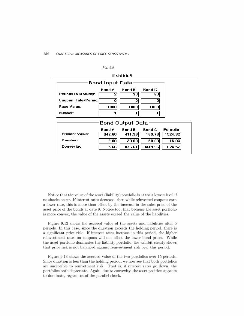
The firm wants to hedge these liabilities by purchasing an appropriateportfolio of bonds shown in Figure 9.9. The firm chooses a portfolio thatmatches the duration of the liability, but has a higher convexity. The specificportfolio, is outlined in Figure 9.10.

Figure 9.11 shows the accrued value of the asset and liability portfoliosafter 9 periods, corresponding to their durations. The values are computedunder various assumptions on the size of a parallel shock that hits the yieldcurve at date 0.


Fig. 9.9

Notice that the value of the asset (liability) portfolio is at their lowest level ifno shocks occur. If interest rates decrease, then while reinvested coupons earna lower rate, this is more than offset by the increase in the sales price of theasset price of the bonds at date 9. Notice too, that because the asset portfoliois more convex, the value of the assets exceed the value of the liabilities.

Figure 9.12 shows the accrued value of the assets and liabilities after 5periods. In this case, since the duration exceeds the holding period, there isa significant price risk. If interest rates increase in this period, the higherreinvestment rates on coupons will not offset the lower bond prices. Whilethe asset portfolio dominates the liability portfolio, the exhibit clearly showsthat price risk is not balanced against reinvestment risk over this period.

Figure 9.13 shows the accrued value of the two portfolios over 15 periods.Since duration is less than the holding period, we now see that both portfoliosare suceptible to reinvetment risk. That is, if interest rates go down, theportfolios both depreciate. Again, due to convexity, the asset position appearsto dominate, regardless of the parallel shock.

CHAPTER 8: IMMUNIZATION AND TWIST RISK 185

Fig. 9.10

9.10 IMMUNIZATION AND TWIST RISK

The above linear programming problem produces a portfolio of bonds thatis most convex, and hence most likely to produce surplus cash flows at thedate of the liability. However, something should concern you. From the aboveanalysis it looks like we can purchase high convex bonds, and sell low convexbonds with the same duration in such a way that our initial net investmentis zero, but the value in the future will be guaranteed to be nonnegative inall states and positive in most. That is, there is a delightful riskless arbitragestrategy here. Where is the problem?

Recall that we assumed that the yield curve was flat and that the shockto the curve was a parallel shock. If this actually occurred, then indeed,there would be riskless arbitrage strategies. However, the yield curve may not


Fig. 9.11

undergo a parallel shift. One might surmize that the above portfolio strategyof buying high and selling low convexity bonds is very susceptible to shocks inthe yield curve that are not parallel. This suspicion turns out to be correct.

The risk neglected by assuming parallel yield curve shifts is referred to astwist risk. We now consider a measure of twist risk. Exhibit 14 below showsthe cash flows of two portfolios of bonds having the same duration as thetarget. Portfolio A is a barbell portfolio while portfolio B is closer to a bulletportfolio. As before the liability date is m.

While portfolio A has greater convexity than portfolio B, it is riskier. To seethis, consider what happens if interest rates change in an arbitrary nonparallelway. Suppose short rates decline and long rates increase. The accrued valuesof A and B would be lower than the target value because of lower reinvestmentrates and lower bond prices. However, the loss in A would be greater than B.First, lower reinvestment rates are experienced for longer periods with A, andsecond, the price risk at m is greater for the long bond in A than that in B.


Fig. 9.12


Fig. 9.13

The bullet portfolio has much less exposure to a change in shape of theterm structure. Indeed, if the bond portfolio immunizing the liability has noreinvestment risk, then the liability is completely immunized regardless of theshift in interest rate structure. When there are high dispersion of cash flowsaround the horizon date, as in the barbell portfolio, the portfolio is exposedto higher reinvestment risk, and hence greater immunization risk. Near bulletportfolios are therefore subject to less twist risk than barbell portfolios. Ameasure of twist or immunization risk is given by M2 where

M2 =n∑

i=1

wi(t − m)2

where wi is the present value of the ith cash flow relative to the bond price,and m is the duration of the bond. Clearly, M2 = 0 only if the weights areall zero except at date m where W1 = 1. In this case the portfolio consists ofa discount bond that perfectly immunizes the liability regardless of the typesof shocks in the interest rate term structure. In general, the larger M2 , thegreater the variability of cash flows around the “target” date m. Fong and


Vasicek have shown that the lower the M2 risk measure, the lower the riskis against nonparallel shifts in the yield curve. To minimize this twist riskan immunizing portfolio can be constructed by solving the following linearprogram:

Minimize∑K

i=1 αiM2i

subject to∑K

i=1 αiDi = m∑K

i=1 αi = 1

The first constraint states that the duration must be m. The second con-straint forces the sum of the fractions of wealth invested in the K bonds toadd up to 1. Additional constraints, such as convexity and nonnegativityconstraints, could be included.

Example

In our previous problem, if the shocks are not parallel shocks, then the valueof the liabilities after 9 periods could exceed the value of the assets. A betterhedge against interest rate shocks would be not only to duration match butalso to convexity match.


9.11 DURATION AND CONVEXITY USING CONTINUOUSLY

COMPOUNDED YIELDS TO MATURITY

In our analysis so far, we assumed the compounding interval was the sameas the time between cash flows. Let y∗ represent the annualized yield tomaturity, and assume that compounding takes place k times a year. Then

B0 =m∑

i=1

CFi

(1 + y∗/k)i

D =m∑

i=1

(i/k)wi

Dm =D

(1 + y ∗ /k)

where wi is the contribution of the present value of the ith cash flow to thebond price. Here B0 is the bond price and D is the duration in years.

Notice that as k → ∞, y ∗ /k → 0 and Dm = D. In this case the modifica-tion of duration to measure price sensitivity becomes unnecessary. Indeed, forcontinuously compounded yields, duration and modified duration are identi-cal.

To see this recall

B =m∑

i=1

CFi × e−tiy

HencedB

dy= −

m∑

i=1

tiCFi × e−tiy

anddB

B= (

m∑

i=1

iwi)dy

where

wi =e−ytiCFi

B=

P (0, ti)CFi

B

9.12 DURATION WITH NONFLAT TERM STRUCTURES

So far we have assumed that the term structure of interest rates is flat at y.Specifically, y(0, t) = y. Then, when a shock ocurrs to the term structure, all

CHAPTER 8: DURATION DRIFT AND DYNAMIC IMMUNIZATION STRATEGIES 191

yields move the same amount. Hence after the shock all yields to maturityare y + ∆y. We have seen that if such shocks were the only shocks to occur,then there would be arbitrage opportunities. Hence limiting yield curves tobe flat, and shocks to be parallel, is unreasonable. Actually, for the analysisin this chapter, we do not need yield curves to be flat. What we do requireis the shock to be the same for all yields. In particular, using continuouslycompounded returns, we have.

B(0) =m∑

i=1

CFi × e−y(0,ti)ti

where y(0, ti) is the actual continuously compounded yield to maturity for thetime period [0, ti] where ti is the time in years to the ith cash flow. Then wecould assume all yields increase by ∆y. Then, the new bond price would be

m∑

i=1

CFi × e−(y(0,ti)+∆y)ti

The duration measure can then be computed by differentiating this equationwith respect to ∆y. This leads to

Dm =m∑

i=1

ti∆twi

where wi = CFiP (0,ti)B0

Example

To Be Done

9.13 DURATION DRIFT AND DYNAMIC IMMUNIZATION

STRATEGIES

As time advances, the duration of the portfolio changes, and the holdingperiod diminishes. Unfortunately, these two values will not decline at thesame rate. Duration, in fact, decreases at a slower rate, a process referred toas duration drift. Hence a portfolio of coupon bonds with duration matching


the original liability period, m, will, after a certain amount of time, t say, havea duration exceeding the target value, m − t. This implies that to maintainan immunized position, the portfolio needs to be periodically readjusted suchthat its duration is reset to the time remaining to the liability payment.

The duration procedures described in this chapter have for the most partassumed yield curves to be flat and shocks to the yield curve have been re-stricted to parallel shifts. In practice, yield curves do not behave this way.Indeed it is unreasonable to assume yields-to-maturity on different assets willchange by the same amount. First, yields to maturity are complex averagesof the underlying spot rates. A given shift in the spot rate curve will result inthe yields to maturity on different assets changing by differing amounts. Sec-ond, yields for different maturities are imperfectly correlated. If short termrates increase by 1%, long term rates typically move by less than 1%. Indeedthe short rate and long rate could move in different directions, causing theyield curve to increase (decrease) in steepness, for example. This twistingshape in the yield curve is not explicitly considered in the previous models.It suggests that the yield curve responds to more than one factor. With morethan one factor causing shocks to the yield curve, more complex durationmodels need to be established. Ideally, these models should be based on morerealistic models of interest rate behavior. A significant body of research hasbeen devoted to this problem, and many alternative duration measures havebeen constructed.3

9.14 DURATION OF FLOATING RATE NOTES.

Consider a floating rate note that pays according to 6 month LIBOR every6 months for n years. LIBOR is determined at the beginning of each periodand paid at the end of the period. Let `[ti, ti+1] represent the Libor rate atdate ti for the time period [ti, ti+1]. The cash flow of N`[ti, ti+1]∆ti occursat date ti+1. We shall assume the face value N is $100. To convert 6 monthLIBOR into a semiannually compounded rate, we have

y

2= `[ti, ti+1]×

Days in period360

We have seen that the price of a floating rate note at date 0, is given by:

VFLOAT = 100P (0, t0) =100

(1 + y/2)p

where p is the fraction of a six month period remaining to the next reset date.

3We shall consider some extensions to the theory in the next chapter.

CHAPTER 8: DURATION FOR INTEREST RATE SWAPS 193

Alternative Development of the FRN Pricing Equation

Assume the maturity of the FRN was 6 months. If the bond equivalent yieldis y, we have:

VFLOAT =100(1 + y/2)

1 + y/2= 100

Now assume the bond has 12 months to go. We know that after 6 monthsthe bond will trade at par. Hence the value of the bond is the present valueof $100 plus the present value of the interest over a reset period. That is:

VFLOAT =100(1 + y/2)

1 + y/2= 100

Repeating this arguement recursively, reveals that at a reset date the FRN isalways set at its face value.

Now consider what happens between reset dates. The final cash flow isgiven by 100(1 + y∗/2) where y∗ was determined at the previous rest point.The price is therefore given by

VFLOAT =100(1 + y∗/2)

(1 + y/2)p

where p is the fraction of a six month period remaining to the cash flow, andy is the bond equivalent yield associated with the current LIBOR rate overthe time to the next reset date.

The Duration of the FRN is therefore given by differentiating the aboveequation with respect to y. The result is:

DFLOAT =p/2

1 + y/2

The modified duration of FRNs therefore range from 0 to 0.5 years. FRNshence behave like fixed rate notes with maturities with less than six monthsremaining to maturity.

9.15 DURATION FOR INTEREST RATE SWAPS

An interest rate swap can be viewed as a long position in a fixed rate noteand a short position in a floating rate note. We can compute the duration ofeach of the legs separately, but we cannot really compute the duration of the


swap, since at the initiation date the value of the swap is zero. In a portfoliocontext, however, the swap can be handled quite effectively.

In practice, it may make more sense to investigate the absolute changein value of the swap to a yield curve shock. For example, the PVBP of aninterest rate swap can be easily obtained.

Example

To be done

9.16 INVERSE FLOATERS

An inverse floating rate note is a FRN, where the rate varies inversely withthe index rate, such as 6 month Libor. In particular,

Rateti = k − `[ti, ti+1]

A floor of zero is placed on this rate to ensure that the number cannot gonegative.

Example

A dealer purchases 100m dollars of a fixed rate bond, that pays 10%coupons semiannually, and place it in trust. The trust then issues a 50mdollar floater and a 50m dollar inverse floater with the floater linked to sixmonth Libor. The rate on the inverse floater is:

10%− Libor.

At each reset/coupon date the trust receives 100 × 0.10/2 = 0.5 milliondollars. In addition the trust is responsible for paying 50y∗/2 million dollarson the floaters and 50(0.10−y∗)/2 million dollars on the inverse floaters. Herey∗ represents the 6 month Libor rate. The net sum the trust is responsiblefor is 50 × 0.05 = 0.25 million dollars.

The buyer of an inverse floater can be viewed as long the fixed bond andshort the floater. Ignoring the floor, we therefore have:

VINV ERSEFLOAT = VFIXED − VFLOAT

CHAPTER 8: CONCLUSION 195

The duration of an inverse floater can now easily be determined. Let

wFIXED =VFIXED

VINV ERSE FLOAT

wFLOAT =VFLOAT

VINV ERSE FLOAT.

Then, the duration of the inverse floater is:

DINV ERSEFLOATER = wFLOAT DFLOAT + wFIXEDDFIXED

9.17 CONCLUSION

This chapter has reviewed the basic concepts of risk management measures inthe bond market. The most common measures of the sensitivity of default freebonds to interest rate changes is captured by modified duration and convexity.The assumption here is that when shocks occur in the yield curve they areparallel shocks. Applications of these measures were provided. In particularwe investigated how portfolio managers can use duration and convexity toimmunize debt obligations.


9.18 REFERENCES

This chapter draws very heavily from the presentation of duration in thetextbook Numerical Methods in Finance, by Simon Benninga. This book andaccompanying software are highly recommended. Another excellent discussionof duration is given by Dunetz and Mahoney. For a comprehensive treatmentof duration, the text by Bierwag is recommended.

Benninga, S. ”Numerical Methods in Finance”, MIT Press, 1989.

Bierwag, G.O., 1977, ”Immunization, Duration, and the Term Structure ofInterest Rates”, Journal of Financial and Quantitative Analysis, Vol.12, 725-741.

Bierwag, G.O., 1987, Duration Analysis: Managing Interest Rate Risk, Cam-bridge, MA: Ballinger.

Bierwag, G.O., I. Fooladi and G.S. Roberts, 1993, ”Designing an ImmunizedPortfolio: Is M-squared the Key?”, Journal of Banking and Finance, 17,1147-1170.

Bierwag, G.O., G.G. Kaufman, and C. Khang, 1978, ”Duration and BondPortfolio Analysis: An Overview”, Journal of Financial and Quantita-tive Analysis, 13, 671-685.

Bierwag, G.O., G.G. Kaufman, C. Latta and G.S. Roberts, 1987, ”Useful-ness of Duration in Bond Portfolio Management: Response to Critics”,Journal of Portfolio Management.

Bierwag, G.O, G.C. Kaufman, R. Schweitzer and A. Toevs, 1981, ”The Artand Risk Management in Bond Portfolios”, Journal of Portfolio Man-agement, Spring, 27-36.

Bierwag, G.O., G.C. Kaufman and A. Toevs, 1982, ”Single-Factor DurationModels in a General Equilibrium Framework”, Journal of Finance, 37,325-338.

Chambers, D.R., 1984, ”An Immunization Strategy for Future Contracts onGovernment Securities”, The Journal of Future Markets, 4, 173-188.

Chambers, D.R. and W. Carleton, ”A Generalized Approach to Duration”,Research in Finance, Vol. 7, 1988, 163-181, JAI Press Inc.

Chua, J., 1984, ”A Closed-Form Formula for Calculating Bond Duration”,Financial Analysts Journal, May/June, 76-78, and G.C. Babcock, ”Dru-ation as a Weighted Average of Two Factors”, Financial Analysts Jour-nal, March/April 1985, p.75.

CHAPTER 8: REFERENCES 197

Dunetz, M. and J. Mahoney, ”Using Duration and Convexity in the Analysisof Callable Bonds”, Financial Analysts Journal, May 1988, 53-72.

Fong, H.G. and F.J. Fabozzi, 1985, Fixed Income Portfolio Management,Homewood, IL: Dow-Jones Irwin.

Fong, H.G. and O. Vasicek, ”The Tradeoff Between Return and Risk inImmunized Portfolios”, Financial Analysts Journal, September-October1983, 73-78.

Fong, W.J. and G.A. Vasicek, 1983, Return Maximization for ImmunizedPortfolios”, in G.O. Bierwag, G. Kaufman and A. Toevs, eds., Innova-tions in Bond Portfolio Management, Greenwich, CT: JAI Press, 227-238.

Ingersoll, J.E., J. Skelton and R.L. Weil, 1978, ”Duration Forty Years Later”,Journal of Financial and Quantitative Analysis, 13, 627-652.

Livingston, M., 1979, ”Measuring bond Price Volatility”, Journal of Finan-cial and Quantitative Analysis, 14, 343-349.

Macaulay, F.R., 1938, Some Theoretical Problems Suggested by the Move-ments of Interest Rates, Bond Yields, and Stock Prices in the U.S. Since1856, New York: National Bureau of Economic Research.

Nawalkha, S.K. and N.J. Lacey, 1988, ”Closed-Form Solutions of Higher-Order Duration Measures”, Financial Analysts Journal, November-December,82-84.

Prisman, E.Z. and M.R. Shores, 1988, ”Duration Measures for Specific TermStructure Estimates and Applications to Bond Portfolio Immunization”,Journal of Banking and Finance, 12, 493-504.


9.19 EXERCISES

1. The term structure is flat at 8%. Consider an 8% coupon bond withsemiannual payouts that matures in 10 years. If yields increased by 1basis point (y = 8.01%) what would be the effect on price? If the yieldcurve was flat at 9% and increased by 1 basis point, would the priceeffect be bigger or smaller. Explain.

2. A bond has 2-years to maturity, pays semiannual coupons, and a facevalue of $1,000. The coupon is 7%, and the yield-to-maturity is 8%.

(a) Compute the price of the bond.

(b) Compute the duration, and modified duration of the bond.

(c) Compute the convexity of the bond.

3. Assume the yield on the bond changes from 8% to 8.05%.

(a) Using the bond pricing equation, compute the new price of thebond, and then establish the change in the bond price.

(b) Using the linear approximation, compute the change in the bondprice.

(c) Using the quadratic approximation, compute the change in thebond price.

(d) Compare the answers in (b) and (c) to that in (a) and draw con-clusions.

4. Repeat problem (2), but this time assume the yield changes from 8 to10%.

5. A discount bond is available with a maturity of 6 years. The annualizedyield-to-maturity of this bond is 7% (computed on a semi annualizedbasis) and the face value is $1000.

(a) Compute the price of this bond.

(b) Compute the duration, modified duration and convexity of thisbond.

CHAPTER 8: EXERCISES 199

6. A trader has an obligation of $10m due in 4 years. The trader decidesto purchase units of the bond in question (1) and the bond in question(3), and wants to choose the portfolio that has a duration equal to thatof the liability. Establish the required portfolio.

7. A 8 year bond has annual coupons. The coupon is 10%, the face valueis $1000, and the current yield curve is flat at 10%.

(a) Compute the duration of the bond.

(b) Assume the yield curve increased from 10% to 10.5%, and remainedunchanged for two years, at which time the bond was sold. Assumeall coupons were reinvested. What would be the total accrued valueof the account.

(c) Another coupon bond with a duration of two years was available.Assume the number of units purchased of this bond were chosen sothat the initial investment was equal to the inital value of the abovebond. After two years, would the accrued value of the account bemore insulated from an immediate parallel shift in the yield curve.Explain.

8. Assume the yield curve is flat at 10%. (y = 10%) Consider the following3 bonds:

Bond A B C

Maturity (Years) 2 5 8Coupon 8% 10% 2%Face Value 1000 1000 1000

(a) Compute the prices of the 3 bonds.

(b) Compute the duration, modified duration and convexity of the 3bonds.

(c) Use bonds A and B to construct a portfolio that has a duration of3 years.

(d) Use bonds A and C to construct a portfolio that has a duration of3 years.

(e) Of the two portfolios constructed in (c) and (d), which one is moreconvex. If the trader wanted a duration of 3 years to immunize anobligation due in 3 years, which of the above two portfolios would


you recommend? Explain.

(f)Of all the portfolios of bonds A, B and C, find the portfolio that max-imizes convexity. Assume the trader is not allowed to sell bondsshort. That is, solve the linear programming problem for the max-imum convexity problem but include in your constraints, the factthat all the weights of the portfolio must be nonnegative.

(g) Compute the twist risk for each bond, and then identify the min-imum twist risk portfolio that has a duration of 3 years. Again,in your linear programming formulation, assume the trader is onlyconcerned with portfolio weights that are non-negative.

(h) Compute the portfolio that maximizes twist risk, subject to theduration and nonnegativity constraints. Compare this portfolio tothat obtained in (f).

CHAPTER 8: EXERCISES 201

AppendixDerivation of Modified Duration and Convexity

Differentiating the bond pricing equation leads to

dB/dy = −m∑

t=1

tCFt

(1 + y)t+1

Dividing both sides by the bond price yields

dB

dy

1B

=−

∑mt=1

tCFt

(1+y)t

B(1 + y)

ordB

dy

1B

= −D1

1 + y

which leads to the duration equation.

Differentiating the bond pricing equation two times, leads to:

d2B

dy2=

m∑

t=1

t(t + 1)CFt

(1 + y)t+2

from which the convexity equation follows.

Finally, use Taylor’s expansion of B(y):

B(y + ∆y) ≈ B(y) +dB

dy∆y +

12

d2B

dy2(∆y)2

Now substituting in the modified duration and convexity exprtessions leadsto the quadratic approximation equation.

Date post:	16-Jul-2018
Category:	Documents
Upload:	vuhanh
View:	216 times
Download:	0 times

Measures of Price Sensitivity 1 - Faculty &...

Documents