arX

iv:1

009.

3977

v3 [

stat

.AP]

19

Oct

201

0

Measuring and implementing the bullwhip effect under

a generalized demand process

Marlene Silva Marchenaa,

aDepartment of Electrical Engineering, Pontifical Catholic University of Rio de Janeiro.

Rua Marques de Sao Vicente, 225. Edificio Cardeal Leme, Gavea, Rio de Janeiro, Brazil.

Cep: 22451-900 Phone: +55 21 35271202 Fax:+55 21 35271232

Abstract

The measure of the bullwhip effect, a phenomenon in which demand vari-ability increases as one moves up the supply chain, is a major issue in SupplyChain Management. Although it is simply defined (it is the ratio of theunconditional variance of the order process to that of the demand process),explicit formulas are difficult to obtain. In this paper we investigate the theo-retical and practical issues of Zhang [Manufacturing and Services OperationsManagement 6-2 (2004b) 195] with the purpose of quantifying the bullwhipeffect. Considering a two-stage supply chain, the bullwhip effect is measuredfor an ARMA(p,q) demand process admitting an infinite moving average rep-resentation. As particular cases of this time series model, the AR(p), MA(q),ARMA(1,1), AR(1) and AR(2) are discussed. For some of them, explicit for-mulas are obtained. We show that for certain types of demand processes, theuse of the optimal forecasting procedure that minimizes the mean squaredforecasting error leads to significant reduction in the safety stock level. Thishighlights the potential economic benefits resulting from the use of this timeseries analysis. Finally, an R function called SCperf is programmed to cal-culate the bullwhip effect and other supply chain performance variables. Itleads to a simple but powerful tool which could benefit both managers andresearchers.

Keywords: Supply chain management, Bullwhip effect, ARMA,Order-Up-To, Safety stock.

Email address: marchenamarlene@gmail.com, marchena@ele.puc-rio.br

(Marlene Silva Marchena)

Preprint submitted to Elsevier October 20, 2010

1. Introduction

In recent years, companies in various industries have been able to signifi-cantly improve their inventory management processes through the integrationof information technology into their forecasting and replenishment systems,and by sharing demand-related information with their supply chain partners,Aviv (2003). However, despite the benefits resulting from the implementationof the above practices, inefficiencies still persist and are reflected in relatedcosts.

The bullwhip effect, defined as the increase in variability along the sup-ply chain, is a frequent and expensive phenomenon identified as a key driverof inefficiencies associated with Supply Chain Management (SCM). It dis-torts the demand signals, which causes instability in the supply chain, andincreases the cost of supplying end-customer demand.

Forrester (1958) was the first to popularize this phenomenon. Inspiredby Forrester’s work, several researchers have studied the bullwhip effect.Sterman (1989) used the Beer Game, the most popular simulation of a simpleproduction and distribution system, to demonstrate that the bullwhip effectis a significant problem with important managerial consequences. It resultsin unnecessary costs in supply chains such as inefficient use of production,distribution and storage capacity, recruitment and training costs, increasedinventory and poor customer service levels (Metters (1997) and Lee et al.(1997b)).

Lee et al. (1997a,b) identified four main causes of the bullwhip effect:demand forecasting, order batching, price fluctuation and supply shortages.Of these, demand forecasting is recognised as one of the most important sincethe inventory system is directly affected by the forecasting technique chosen.Three popular forecasting methods are commonly used: the Minimum MeanSquared Error (MMSE), Moving Average (MA) and Exponential Smoothing(ES).

Chen et al. (2000a) quantify the bullwhip effect considering the MA fore-cast method for a simple two-stage supply chain and a first-order autoregres-sive demand process, AR(1). The authors show that the bullwhip effect is inpart due to the effects of demand forecasting. Therefore, given complete ac-cess to customer demand information for each stage of the supply chain, thebullwhip effect can be significantly reduced. However, they also show thatthe bullwhip effect will exist even when demand information is shared by allstages of the supply chain and all stages use the same forecasting technique

2

and the same inventory policy. In similar work Chen et al. (2000b) quantifythe bullwhip effect considering this time the ES forecast and two different de-mand processes: AR(1) demand process and a demand process with a lineartrend. In both works, the authors recognize an important limitation of theirresults: the models considers only non-optimal forecasting methods. Theauthors justify this limitation saying that ES and MA are commonly usedin practice. Users are in general less familiar and less satisfied with moresophisticated methods like time series techniques.

Zhang (2004a) investigates the impact of MMSE, MA and ES forecastingmethods on the bullwhip effect for a simple inventory system in which AR(1)demand process describes the customer demand and an Order-Up-To (OUT)inventory policy is used. The study shows that different forecasting methodslead to bullwhip effect measures with distinct properties in relation to lead-time and the underlying parameters of the demand process. The authorshows that MMSE forecasting method leads to the lowest inventory cost.This result is not surprising since MMSE method is optimal when the demandmodel is known to be an AR(1) process. On the other hand, if the demandstructure is not well known, the MA or ES method may perform better thanthe MMSE method because they are more flexible.

Another aspect studied in relation of the bullwhip effect is the demandprocess. A variety of time-series demand models have appeared in the liter-ature of inventory control and SCM. By far, the AR(1) process is the mostfrequently adopted demand model to study the bullwhip effect (Chen et al.(2000a,b), Lee et al. (1997a,b) and Zhang (2004a)). Recent works use moresophisticated time series models like ARMA and ARIMA (Box and Jenkins,1970) to have more realistic demand models. Luong and Phien (2007) usean AR(2) and a general AR(p) model; Duc et al. (2008) use an ARMA(1,1)model. In all these models an analytical derivation of the bullwhip effectmeasure is presented and the effects of the autoregressive coefficient on thebullwhip effect is investigated.

Zhang (2004b) uses an ARMA(p,q) model to study the demand evolu-tion in supply chains. The author shows that the order history preservesthe autoregressive structure of the demand. Zhang’s work identifies an im-portant application of this result relating to the quantification of the bull-whip effect. In this paper, inspired by Zhang’s work, we study the the-oretical and practical issues in order to measure the bullwhip effect for ageneralized demand process. In addition, we programmed a function in R

3

(R Development Core Team, 2010), called SCperf1, which implements thebullwhip effect and others supply chain performance variables. It is wellknown that measuring the bullwhip effect is difficult in practice but theSCperf function overcomes this problem thanks to the help of an R func-tion (ARMAtoMA) which converts an ARMA process into an infinite movingaverage process. As far as practical applications are concerned, the economicimplications of this phenomenon on the inventory cost have been considered.

Our contributions to this subject can be described as follows: first, thisstudy hopes to improve the understanding of time series techniques. Second,we show that for certain types of demand processes the use of the opti-mal forecasting procedure that minimizes the mean squared forecasting errorleads to significant reduction in the safety stock level. This highlights thepotential economic benefits resulting from the use of this time series analysis.Finally, the SCperf function leads to a simple but powerful tool which canbe helpful for the study of this phenomenom and other supply chain researchproblems.

The structure of our paper is as follows. The next section presentsthe inventory model. Section 3 presents a general ARMA(p,q) case withARMA(1,1), MA(q), AR(p), AR(1) and AR(2) as particular cases. Next theeconomic implications are shown. The final section summarizes the mainresults of the research.

2. Inventory model

In this paper we consider a simple supply chain model for a single itemand an OUT inventory policy in which the retailer determines a target levelor OUT level and, for every review period, places an order sufficient to bringthe inventory position back to this level. As did Chen et al. (2000b), weconsider that the ordered quantity made in period t is received at the startof period t + L where L is defined to be a fixed lead time plus the reviewperiod, i.e., L is the lead time plus 1. For instance, in the case of zero leadtime, L = 1. Shortages are back-ordered and no fixed ordering cost exists.In the remainder of the paper L will call the lead time. This choise is madefor sake of brevity, and should not create confusion.

The sequence of events during a replenishment cycle for each period t canbe described as follows: the retailer receives orders made L periods ago; the

1See the supplementary material

4

demand dt is observed and satisfied; the retailer observes the new inventorylevel and finally places an order Ot to the supplier. As a consequence of thissequence of events, the ordered quantity can be written as:

Ot = St − St−1 + dt, (1)

where St represents the OUT level in period t, i.e., the inventory position atthe beginning of period t. Note that in the above expression, we have implic-itly assumed that the order quantity can be negative, i.e., returning itemsare allowed at no costs. This unpleasant feature is needed for tractability.However, the free-return assumption becomes negligible when the demandmean is sufficiently large. Further detail about this assumption can be foundin Lee et al. (2000) and Chen and Lee (2009).

Under the OUT policy, the OUT level St can be estimated from theobserved demand as:

St = DLt + zσL

t , (2)

where DLt =

∑L

τ=1 dt+τ is an estimate of the mean demand over L periodsafter period t, z is the safety factor which is a fixed constant chosen to meet

a required service level and σLt =

√

V ar(DLt − DL

t ) is an estimate of thestandard deviation of L periods forecast error. An OUT policy of this formis optimal when the demand came from a normal distribution and there isno setup or fixed order cost.

As Chen et al. (2000b) mention, if the retailer follows an OUT policyof the form St = DL + zσL, where DL is the known mean and σL is thestandard deviation of the demand over L periods, then the OUT level in anyperiod is constant and, consequently, the order is equal to the last observeddemand. Therefore, there is no bullwhip effect. However, these values are, ingeneral, unknown and the retailer must estimate them using some forecastingtechnique. Note that the introduction of forecasting values in the calculationof St is one of the main causes for the variability increase along the supplychain or, in other words, the bullwhip effect.

The demand forecast is performed here by using the MMSE method.It was shown that, for an ARMA process, the MMSE forecast for periodt + τ is the conditional mean given the observed information2. Let t =

2Box and Jenkins, 1970, pp.128.

5

{dt, dt−1, ....} be the information set which represents all the informationavailable until period t. Hence, the demand forecast for τ periods ahead isgiven by E(dt+τ |t).

In order to quantify the bullwhip effect we combine (1) and (2) to rewritethe order quantity as:

Ot = (DLt − DL

t−1) + z(σLt − σL

t−1) + dt. (3)

We show later in the paper (see Lemma A.1) that the standard deviationof lead-time forecast error remains constant over time for an ARMA(p,q)demand process. Hence, σL

t = σLt−1 and the order quantity given in (3)

becomes

Ot = (DLt − DL

t−1) + dt. (4)

Let M be the measure for the bullwhip effect. Since M can be obtainedfrom the ratio between the unconditional variance of the order process tothat of the demand process, we have

M =V ar(Ot)

V ar(dt). (5)

Note that M is calculated by using the variances from both side of Equation(4). The fact thatM = 1 means that there is no variance amplification, whileM > 1 means that the bullwhip effect is present. On the other hand, M < 1means that the orders are smoothed if compared with the demand. The lastcase is less common since it is unlikely to have a situation where stages upthe supply chain have a better representation of the customer demand thanthe first stage (i.e., the retailer).

In what follows, the corresponding bullwhip effect measure is derived for ageneral ARMA(p,q) demand process and some particular cases are discussed.Since the calculation is complex, we cannot always express this measure in aclosed form. In this context, the SCperf function was developed to overcomethis computational difficulty.

6

3. ARMA(p,q) case

The demand process, dt, seen by the retailer, is described by a stationaryARMA(p,q) process as follows3:

dt = µ+ φ1dt−1 + · · ·+ φpdt−p + ǫt + θ1ǫt−1 + · · ·+ θqǫt−q, (6)

where µ is a nonnegative constant, ǫt is i.i.d. normally distributed, withmean zero and variance σ2

ǫ , p is the autoregressive order of the process, q isthe moving average order of the process, φj is the autoregressive coefficient,and θj denotes the moving average coefficient. It is often useful to express(6) in terms of the lag operator, B, where Bkdt = dt−k. In order to do so, letφ(B) = 1− φ1B − · · · − φpB

p and θ(B) = 1 + θ1B + · · ·+ θqBq. Hence, the

demand process in (6) can be expressed as:

φ(B)dt = µ+ θ(B)ǫt,

where φ(B) and θ(B) are known as the autoregressive and the moving averagepolynomials in the lag operator of degree p and q. If we substitute the lagoperator by a constant z, we get the characteristic equations:

φ(z) = 1− φ1z − φ2z2 − · · · − φpz

p

andθ(z) = 1 + θ1z + θ2z

2 + · · ·+ θqzq.

The process is called the autoregressive process of order p, AR(p), if θ(z) = 1and a moving average process of order q, MA(q), if φ(z) = 1. We assumethat the process described in (6) is invertible and covariance stationary, i.e.,the roots of the equations θ(z) = 0 and φ(z) = 0 must be outside the unitcircle. To avoid the problem of parameter redundancy, it is assumed that thetwo characteristic equations share no common roots.

It is important to note that the constant z in the above equations isdifferent from the constant used to define the safety factor. We have chosen

3Our representation differs from some works where the MA model is written withnegative coefficients, i.e., dt = µ + φ1dt−1 + · · · + φpdt−p + ǫt − θ1ǫt−1 − · · · − θqǫt−q.We chose this representation to be in accordance with the R software which was used toimplement the bullwhip effect.

7

this notation to be in accordance with time series notation and we hopethat this will not cause any future confusion. Using stationarity and takenexpectations in (6) directly it can be found that the mean of ARMA(p,q)demand process is defined by

µd =µ

1− φ1 − · · · − φp

. (7)

It is known from time series theory that a stationary ARMA(p,q) demandprocess under the above conditions can be written as an infinite movingaverage process of its errors, MA(∞), that is,

dt = µd + Σ∞j=0ψjǫt−j , (8)

where µd is defined as in Equation (7) and the sequence {ψj} in (8) is de-

termined by the relation ψ(z) =∑∞

j=0 ψjzj = θ(z)

φ(z), or equivalently by the

identity

(ψ0+ψ1z+ψ2z2+· · · )(1−φ1z−φ2z

2−· · ·−φpzp) = (1+θ1z+θ2z

2+· · ·+θqzq).Equating coefficients of zj , j = 0, 1, ..., we find that

ψj =

p∑

k=1

φkψj−k + θj for j ≥ 1, (9)

where θ0 = 1, θj = 0 for j > q, and ψj = 0 for j < 0. Note that equation (9)is a recursive equation. Therefore, the ψ-weights satisfy the homogeneousdifference equation given by

ψj −p∑

k=1

φkψj−k = 0, j ≥ max(p, q + 1), (10)

with initial conditions given by equation (9). From homogeneous differenceequation theory the general solution for equation (10) can be read off directlyas:

ψj = c1z−j1 + · · ·+ crz

−jp , (11)

where z1, .., zp are distinct roots of the polynomial φ(z) and ck, for k =1, 2, ..., p are constants which depend on the initial conditions.4 Now, from

4In the case of the repeated root, the solution is different. See Shumway and Stoffer(2006) for a brief and heuristic account of the topic. For details about homogeneousdifference equation theory the reader is referred to Mickens (1987).

8

equation (8), the variance of the demand process can be expressed as:

σ2d = σ2

ǫ

∞∑

j=0

ψ2j . (12)

It is important to note that the MA(∞) representation depends on aninfinite number of parameters and, consequently, it is not directly useful inpractical applications. On the other hand, Zhang (2004b), using theMA(∞)representation, shows a property, called by the author ARMA-in-ARMA-out(AIAO), which reveals that the order history preserves the autoregressivestructure of the demand and transforms its moving average structure accord-ing to a simple algorithm5. As the author remarks, the practical value ofthe AIAO property lies in its ability to make simpler the measuring of thebullwhip effect.

Proposition 1. (Zhang, 2004b) The retailer’s demand process can be rep-resented by an MA(∞) process with respect to the retailer’s full informationshocks ǫt, as in equation (8). Hence, the retailer’s order Ot to its supplier isgiven by:

Ot = µd +

L∑

j=0

ψjǫt +

∞∑

j=1

ψL+jǫt−j (13)

where the ψj = 0 for j < 0, ψ0 = 1, and ψj =∑p

k=1 φkψj−k + θj for j ≥ 1.

Proof. See Zhang (2004b). �

Proposition 2. For a stationary ARMA(p,q) demand process, the measurefor the bullwhip effect is defined by:

M = 1 +2∑L

i=0

∑L

j=i+1 ψiψj∑∞

j=0 ψ2j

, (14)

where the ψj = 0 for j < 0, ψ0 = 1, and ψj =∑p

k=1 φkψj−k + θj for j ≥ 1.

Proof. Taking the variance of the order quantity, Equation (13), we haveV ar(Ot) = σ2

ǫ (∑L

j=0 ψj)2+σ2

ǫ

∑∞

j=1 ψ2L+j = σ2

ǫ (∑∞

j=0 ψ2j+2

∑L

i=0

∑L

j=i+1 ψiψj).We complete the proof by substituting this result and (12) in (5). �

5Zhang 2004b, pp. 197

9

Proposition 3. The bullwhip effect increases when the lead-time L increasesif and only if ψL+1

∑L

j=0 ψj > 0.

Proof. From equation (14), it is straightforward to see that the bullwhipeffect exists, i.e., M > 1, if and only if

∑L

i=0

∑L

j=i+1 ψiψj > 0. Let g(L) =∑L

i=0

∑L

j=i+1 ψiψj and △g(L) = g(L+ 1)− g(L). Then

△g(L) =∑L+1

i=0

∑L+1j=i+1 ψiψj−

∑L

i=0

∑L

j=i+1 ψiψj = ψ0(∑L+1

j=1 ψj−∑L

j=1 ψj)+

· · ·+ ψL−1(∑L+1

j=L ψj − ψL) + ψLψL+1 = ψL+1

∑L

j=0 ψj . Hence, △g(L) > 0 if

and only if ψL+1

∑L

j=0 ψj > 0. Hence, g(L) is a non-decreasing function of

the lead-time L if and only if ψL+1

∑L

j=0 ψj > 0. �

3.1. ARMA(1,1) caseThe stationary ARMA(1,1) demand process is described as follow:

dt = µ+ φdt−1 + ǫt + θǫt−1. (15)

Stationarity and invertible conditions impose |φ| < 1 and |θ| < 1. It can beshown that the mean and variance of the demand process are µd =

µ

1−φ1

and

σ2d = (1+θ2+2φθ)σ2

ǫ

1−φ2 , respectively.

Proposition 4. For a stationary ARMA(1,1) demand process the measurefor the bullwhip effect is defined by:

M(L, φ, θ) = 1 +2(φ+ θ)(1− φL)

(1− φ)(1 + θ2 + 2φθ)

[

1− φL+1 + θφ(1− φL−1)]

. (16)

Proof. Since the AR polynomial associated with (15) is φ(z) = 1−φz, andits root, say z1, is z1 = φ−1, then the general solution for the ψ-weights canbe written directly from equation (11) as ψj = cφj. From (9) we find thatthe initial conditions are ψ0 = 1 and ψ1 = φ + θ, which combining with thegeneral solution, results in c = (φ+ θ)/φ. Hence, ψj = (φ+ θ)φj−1 for j ≥ 1.Since we know ψj , we can rewrite the follow relations as:

L∑

i=0

L∑

j=i+1

ψiψj = ψ0

L∑

j=1

ψj +

L∑

i=1

L∑

j=i+1

ψiψj

= (φ+ θ)1− φL

1− φ+φ(φ+ θ)2(1− φL)(1− φL−1)

(1− φ)(1− φ2)

=(φ+ θ)(1− φL)

(1− φ)(1− φ2)

[

1− φL+1 + θφ(1− φL−1)]

10

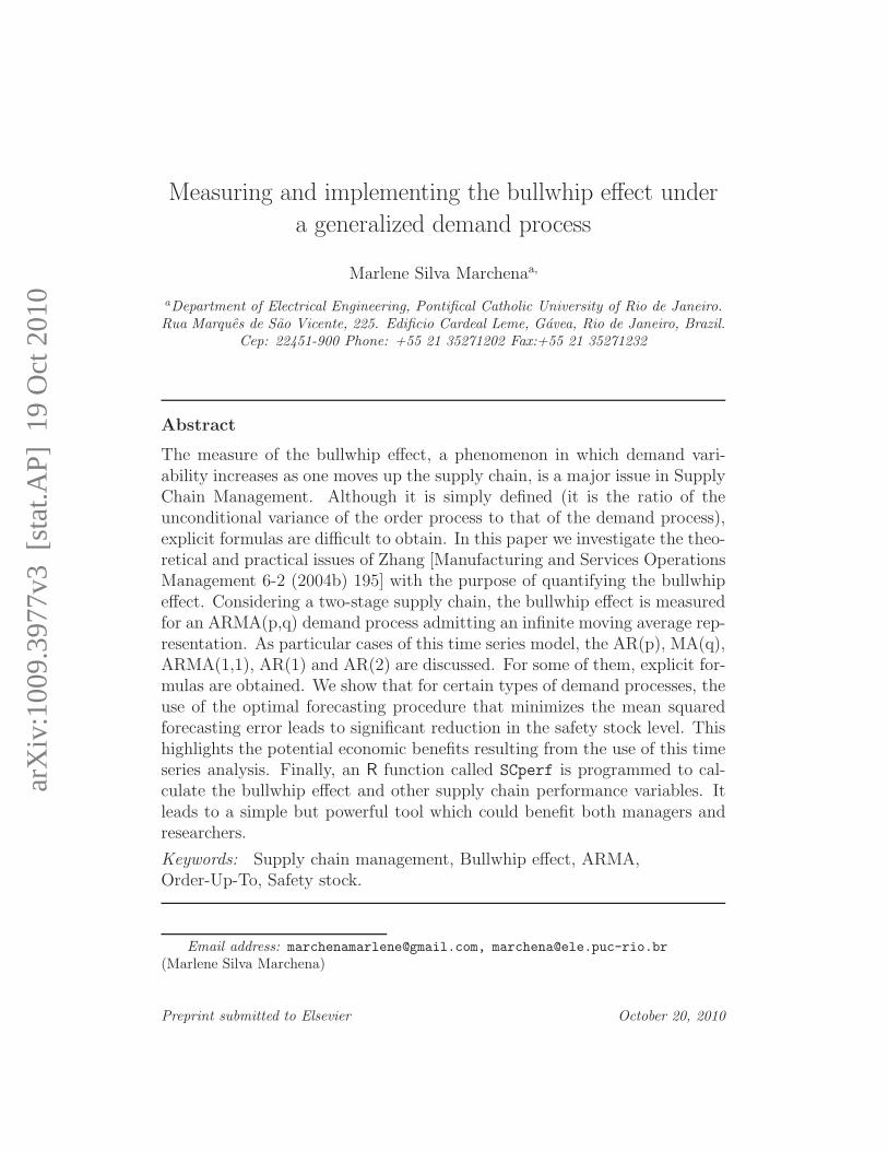
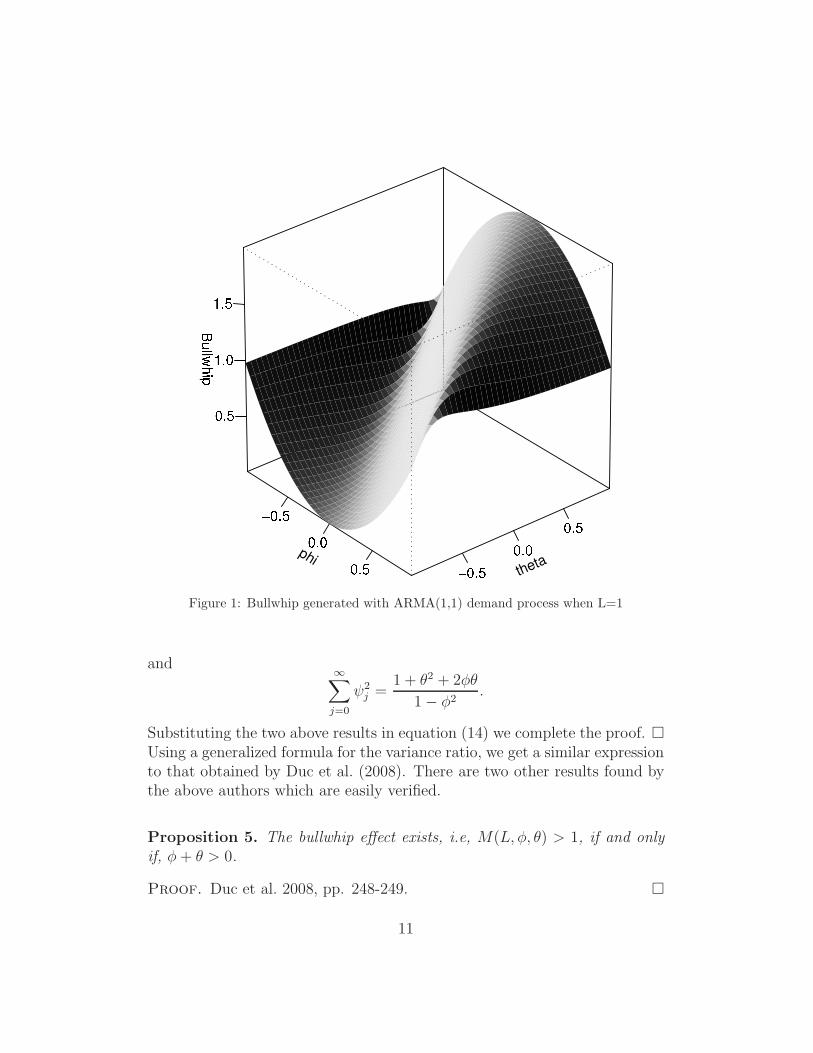
Figure 1: Bullwhip generated with ARMA(1,1) demand process when L=1

and∞∑

j=0

ψ2j =

1 + θ2 + 2φθ

1− φ2.

Substituting the two above results in equation (14) we complete the proof. �Using a generalized formula for the variance ratio, we get a similar expressionto that obtained by Duc et al. (2008). There are two other results found bythe above authors which are easily verified.

Proposition 5. The bullwhip effect exists, i.e, M(L, φ, θ) > 1, if and onlyif, φ+ θ > 0.

Proof. Duc et al. 2008, pp. 248-249. �

11

Proposition 6. The bullwhip effect, measured by M(L, φ, θ), has the follow-ing properties.

(a) If φ > 0, the bullwhip effect increases as L increases.(b) If −θ < φ < 0 and L is an odd number, the larger L is, the smaller

the bullwhip effect is.(c) If −θ < φ < 0 and L is an even number, the larger L is, the larger

the bullwhip effect is.

Proof. Duc et al. 2008, pp. 249. �

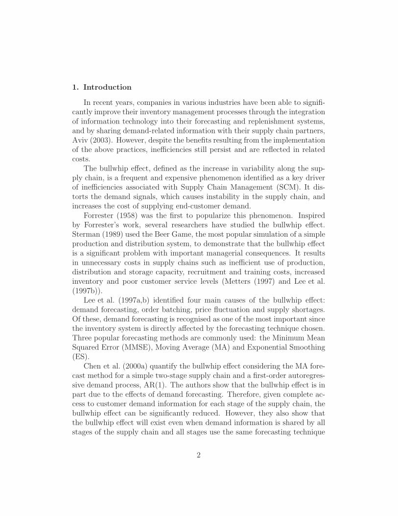
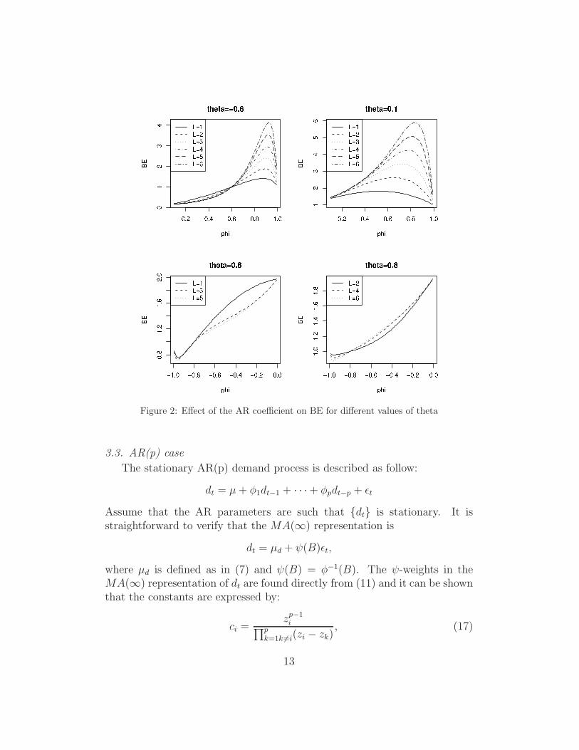
In conclusion the bullwhip effect occurs only when the sum of the ARparameter and the MA parameter is larger than zero ( See Figure 1) and itdoes not always increase when the lead time L increases. In fact, if φ+ θ > 0and φ > 0 the bullwhip effect increases when the lead-time increase. However,if −θ < φ < 0 and L is an odd number, the bullwhip effect becomes smalleras L becomes larger; if −θ < φ < 0 and L is an even number, the bullwhipeffect becomes larger as L becomes larger. Figure 2 represents situationswhere these facts are observed.

3.2. MA(q) case

The MA(q) demand process can be written as

dt = µ+

q∑

j=0

θjǫt−j = µ+ (1 + θ1B + · · ·+ θqBq)ǫt = µ+ θ(B)ǫt.

Since θ(B) is finite, no restrictions on the MA parameters are needed toensure stationarity. Considering q → ∞ the infinite MA representation iswritten as:

dt = µd +∞∑

j=0

ψjǫt−j ,

where ψj = θj for j = 0, 1, .., q and ψj = 0 for j > q. It can be easily seenthat µd = µ and σ2

d = (1+θ21+ · · ·+θ2q)σ2ǫ . Since the above demand process is

i.i.d. the OUT level, St, is constant across all periods. Hence, from Equation(1), Ot = dt, consequently, the bullwhip ratio equals one.

12

Figure 2: Effect of the AR coefficient on BE for different values of theta

3.3. AR(p) case

The stationary AR(p) demand process is described as follow:

dt = µ+ φ1dt−1 + · · ·+ φpdt−p + ǫt

Assume that the AR parameters are such that {dt} is stationary. It isstraightforward to verify that the MA(∞) representation is

dt = µd + ψ(B)ǫt,

where µd is defined as in (7) and ψ(B) = φ−1(B). The ψ-weights in theMA(∞) representation of dt are found directly from (11) and it can be shownthat the constants are expressed by:

ci =zp−1i

∏p

k=1k 6=i(zi − zk), (17)

13

where the constants terms ci sum to the unity, c1+ · · ·+cp = 1, see Hamilton1994, pp. 33-36, for details.

3.4. AR(1) case

The stationary AR(1) demand process is described as follows:

dt = µ+ φdt−1 + ǫt. (18)

Stationarity condition imposes |φ| < 1. Using stationarity it can be shown

that the mean and the variance of the process are µd =µ

1−φ1

and σ2d = σ2

ǫ

1−φ2

1

,

respectively.

Proposition 7. For a stationary AR(1) demand process the measure for thebullwhip effect is defined by:

M(L, φ) = 1 +2φ(1− φL)(1− φL+1)

1− φ(19)

Proof. As in the ARMA(1,1) case, the AR polynomial associated with (18)is φ(z) = 1 − φz, and the root, say, z1, is z1 = φ−1. Using (11) the generalsolution is ψj = c(z1)

−j = cφj1 with ψ0 = 1 and ψ1 = φ as initial conditions.

Combining the general solution with the initial conditions we find ψj = φj .Since ψj = φj , Equation (14) can be expressed as:

M(L, φ) = 1 +2∑L

i=0

∑L

j=i+1 φiφj

∑∞j=0 φ

2j, (20)

where

L∑

i=0

L∑

j=i+1

φiφj =

L∑

i=0

L−i−1∑

k=0

φiφk+i+1 =φ

1− φ

L∑

i=0

φ2i(1− φL−i)

=φ

1− φ

[

1− φ2(L+1)

1− φ2− φL(1− φL+1)

1− φ

]

=φ

1− φ

[

(1− φL)(1− φL+1)

1− φ2

]

and∑∞

j=0 φ2j = 1

1−φ2 . Substituting the two above results in (20) completethe proof. �

14

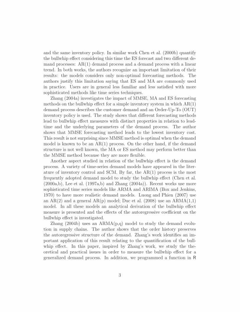
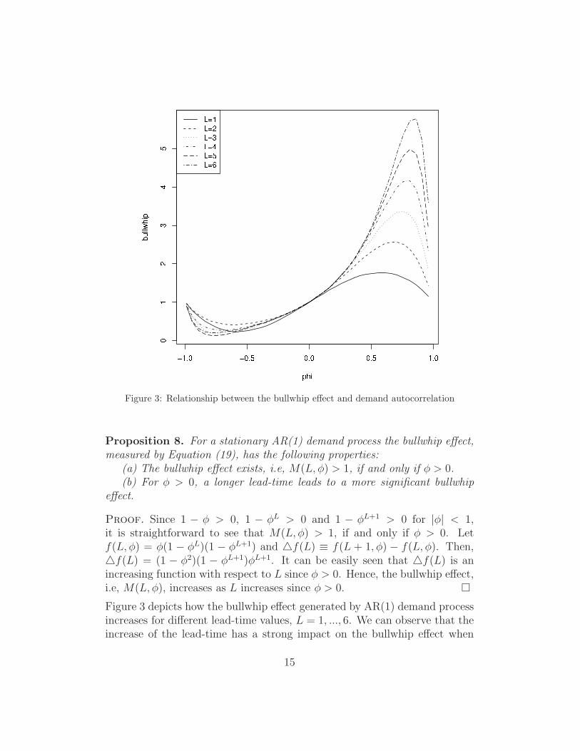
Figure 3: Relationship between the bullwhip effect and demand autocorrelation

Proposition 8. For a stationary AR(1) demand process the bullwhip effect,measured by Equation (19), has the following properties:

(a) The bullwhip effect exists, i.e, M(L, φ) > 1, if and only if φ > 0.(b) For φ > 0, a longer lead-time leads to a more significant bullwhip

effect.

Proof. Since 1 − φ > 0, 1 − φL > 0 and 1 − φL+1 > 0 for |φ| < 1,it is straightforward to see that M(L, φ) > 1, if and only if φ > 0. Letf(L, φ) = φ(1 − φL)(1 − φL+1) and △f(L) ≡ f(L + 1, φ) − f(L, φ). Then,△f(L) = (1 − φ2)(1 − φL+1)φL+1. It can be easily seen that △f(L) is anincreasing function with respect to L since φ > 0. Hence, the bullwhip effect,i.e, M(L, φ), increases as L increases since φ > 0. �

Figure 3 depicts how the bullwhip effect generated by AR(1) demand processincreases for different lead-time values, L = 1, ..., 6. We can observe that theincrease of the lead-time has a strong impact on the bullwhip effect when

15

φ > 0.5 and a less significant one when φ is positive and near zero and one.Therefore, as it was already noted by Zhang (2004a), reduction on the lead-time can reduce the bullwhip effect if the demand autocorrelation is positiveand away from zero and unity in the case of AR(1) demand process.

3.5. AR(2) case

The stationary AR(2) demand process satisfies:

dt = µ+ φ1dt−1 + φ2dt−2 + ǫt (21)

In the AR(2) case, stationarity implies that the roots of φ(z) = 0 lie outsidethe unit circle or, equivalently, the parameters φ1 and φ2 must lie in thetriangular region restricted by φ1 + φ2 < 1, φ2 − φ1 < 1 and |φ2| < 1. It canbe shown that for a stationary AR(2) demand process the mean and variance

of the demand are µ

1−φ1−φ2

and (1−φ2)σ2ǫ

(1+φ2)[(1−φ2)2−φ2

1], respectively.

Proposition 9. Let z1 and z2 be the solutions for the characteristic equationdefined by the AR(2) process. For a stationary AR(2) demand process theψ-weights are defined by:

ψj =z1+j2 − z1+j

1

z1z2(z2 − z1)

Proof. From Equation (10), the general solution for ψj-weights for anAR(2) process is described by:

ψj = c1(z1)−j + c2(z2)

−j (22)

where

z1 =−φ1 +

√

φ21 + 4φ2

2φ2

, (23)

and

z2 =−φ1 −

√

φ21 + 4φ2

2φ2

(24)

are the solutions for the characteristic equation 1− φ1z − φ2z2 = 0. On the

other hand, from Equation (17), the values of the constants are given by:

c1 =z−11

z−11 − z−1

2

(25)

16

and

c2 = − z−12

z−11 − z−1

2

(26)

Finally by replacing (23), (24), (25) and (26) in (22) we find the result. �

Note that the solution for the ψj-weights are a function of the roots of theAR polynomial. In the AR(2) case, the roots can be real if φ2

1 + 4φ2 > 0,or complex if φ2

1 + 4φ2 < 0. In both cases, from a computational point ofview, the solution for the ψj-weights can be found and, therefore, we can geta measure for the bullwhip effect. Since an explicit form for the measure forthe bullwhip effect is difficult to obtain, we investigated the relation of theautoregressive coefficients and lead-time by numerical experimentation. Foran analytical derivation the reader is referred to Luong and Phien (2007).

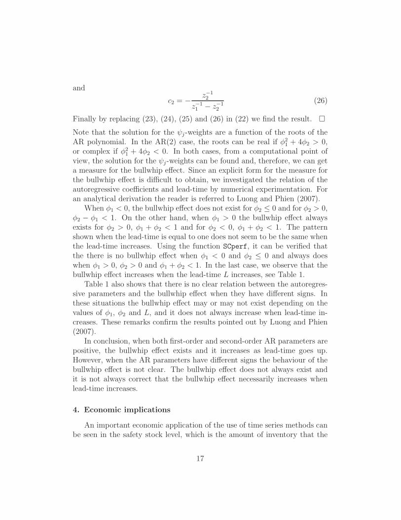
When φ1 < 0, the bullwhip effect does not exist for φ2 ≤ 0 and for φ2 > 0,φ2 − φ1 < 1. On the other hand, when φ1 > 0 the bullwhip effect alwaysexists for φ2 > 0, φ1 + φ2 < 1 and for φ2 < 0, φ1 + φ2 < 1. The patternshown when the lead-time is equal to one does not seem to be the same whenthe lead-time increases. Using the function SCperf, it can be verified thatthe there is no bullwhip effect when φ1 < 0 and φ2 ≤ 0 and always doeswhen φ1 > 0, φ2 > 0 and φ1 + φ2 < 1. In the last case, we observe that thebullwhip effect increases when the lead-time L increases, see Table 1.

Table 1 also shows that there is no clear relation between the autoregres-sive parameters and the bullwhip effect when they have different signs. Inthese situations the bullwhip effect may or may not exist depending on thevalues of φ1, φ2 and L, and it does not always increase when lead-time in-creases. These remarks confirm the results pointed out by Luong and Phien(2007).

In conclusion, when both first-order and second-order AR parameters arepositive, the bullwhip effect exists and it increases as lead-time goes up.However, when the AR parameters have different signs the behaviour of thebullwhip effect is not clear. The bullwhip effect does not always exist andit is not always correct that the bullwhip effect necessarily increases whenlead-time increases.

4. Economic implications

An important economic application of the use of time series methods canbe seen in the safety stock level, which is the amount of inventory that the

17

Table 1: Bullwhip effect generated for different AR(2) demand pro-cess.*

L AR(c(-0.2,0.7)) AR(c(0.6,-0.4)) AR(c(0.7,0.2))

1 0.886667 1.822857 1.3150002 1.222133 1.735086 1.8428503 0.970805 1.170277 2.5128874 1.379174 0.917179 3.2912805 1.051166 0.949074 4.1411056 1.450366 1.060235 5.0358367 1.097494 1.117111 5.9535528 1.464249 1.103809 6.8772219 1.117408 1.072652 7.79354110 1.447477 1.059437 8.692330

* SL=0.95

retailer needs to keep in order to protect himself against deviations fromaverage demand during lead time.

Let SS = zσd√L and SSLT = zσL

t be two safety stock measures. Theformer is traditionally used in some operational research manuals and it isbased on the standard deviation of the demand over L periods, the latter isthe safety stock as defined in (2) and it is based on the standard deviationof L periods forecast error.

Chen et al. 2000b, pp. 271, pointed out that SSLT will be greater thanSS, i.e., using time series analysis, the retailer will hold more safety stock toachieve the same service level. According to the authors this is because SScaptures only the uncertainty due to the random error ǫ and SSLT capturesthis uncertainty plus the uncertainty due to the fact that the mean demandDL

t is estimated by DLt , in our case using the MMSE forecasting method. We

show by numerical experiments that for some special cases SSLT is lowerthan SS regarding lead-time and service level.

Using the SCperf function, it was verified that for ARMA and AR cases,high values on AR parameters and small values of lead-time result in lowerSSLT . However, in general, there is a lead-time value for which this situationis reversed. Table 2 shows the safety stock levels SS and SSLT generated

18

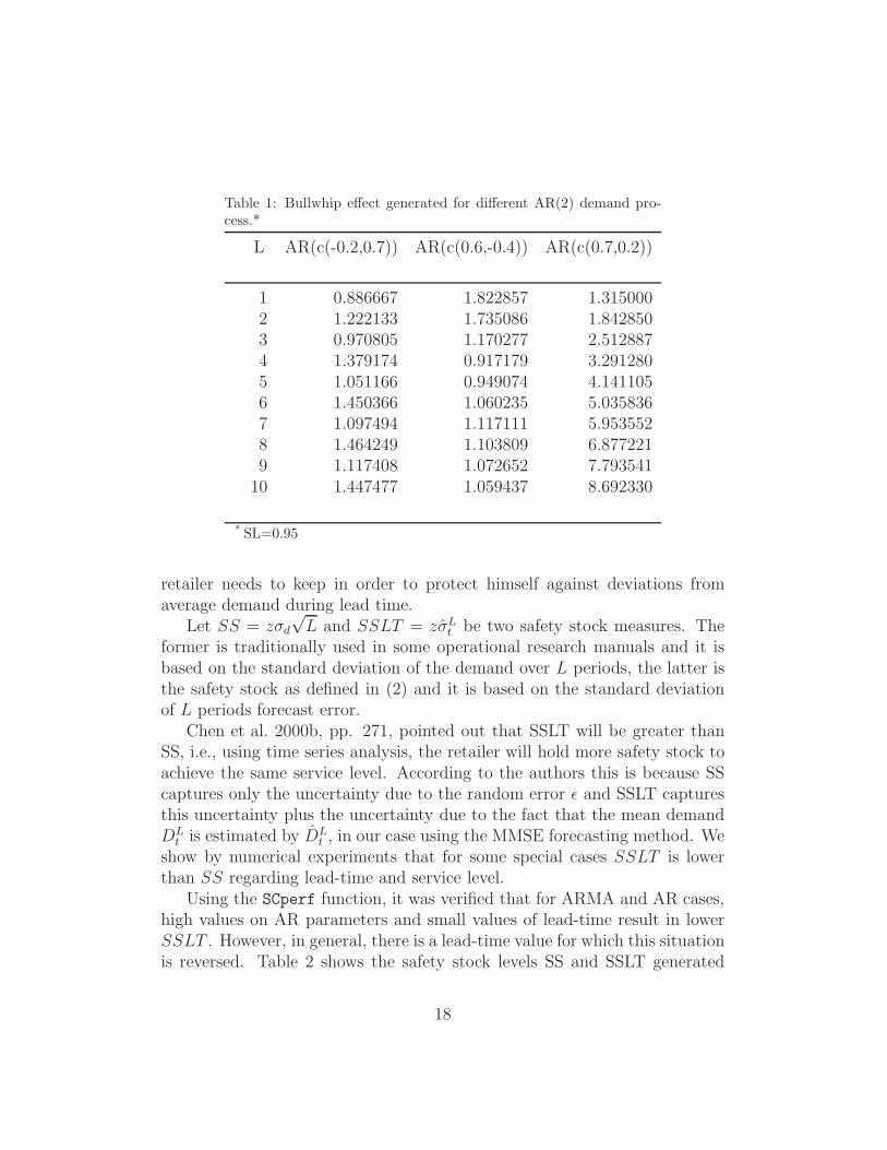
Table 2: Bullwhip, SS and SSLT generatedby ARMA(0.95,0.4) demand process.*

L Bullwhip SS SSLT

1 1.13711 7.299 1.6452 1.44321 10.323 4.2013 1.89270 12.643 7.3044 2.46294 14.598 10.8175 3.13393 16.322 14.6526 3.88802 17.879 18.7457 4.70970 19.312 23.0488 5.58531 20.645 27.5229 6.50289 21.898 32.13710 7.45199 23.082 36.867

* SCperf(0.95,0.4,L,0.95)

by ARMA(0.95, 0.4) demand process and service level equal to 0.95 for tendifferent values of lead-time, L = 1, .., 10. For instance, for L = 2 we haveSS = 10.3 and SSLT = 4.2, a difference of 6 units which represents a savingof 59.2% over SS. Note that this difference decreases when the lead-timeincreases until L = 6 where we have SSLT larger than SS.

It is difficult to know for which value of lead-time SSLT becomes largerthan SS. In general, it depends on the AR parameters of the demand. Fornegative values of the AR parameters, it occurs for lower values of lead-time.Nevertheless, for the AR(2) case the AR parameters present a more complexrelation with the performance of the SSLT. When the first-order and second-order AR parameters are positive, the pattern is the same as the AR andARMA case, that is, SSLT becomes larger than SS for high values of lead-time. Moreover, when the first-order and second-order AR parameters havedifferent signs, it is difficult to determine when the SSLT is better than SSas a measure for the safety stock level.

Table 2 shows that there is a benefit resulting from the use of SSLTinstead of SS as a measure for the safety stock level when regarding the lead-time. This benefit was verified for special demand processes where the ARparameters are high. Moreover, if for those lead-time values where SSLT

19

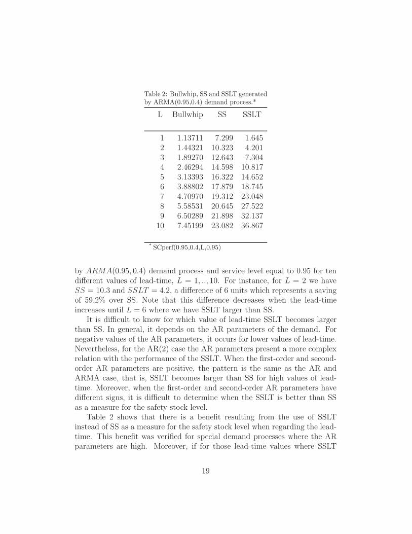
Table 3: SS and SSLT generated by different demand processes

Models Service Level L=1 L=2 L=3SL SS SSLT SS SSLT SS SSLT0.90 5.687 1.282 8.043 3.273 9.850 5.6910.91 5.950 1.341 8.414 3.424 10.305 5.9540.92 6.235 1.405 8.818 3.588 10.800 6.2390.93 6.549 1.476 9.262 3.769 11.343 6.5530.94 6.899 1.555 9.757 3.971 11.950 6.904

ARMA(0.95, 0.4) 0.95 7.299 1.645 10.323 4.201 12.643 7.3040.96 7.769 1.751 10.987 4.471 13.456 7.7740.97 8.346 1.881 11.803 4.803 14.456 8.3520.98 9.114 2.054 12.889 5.245 15.785 9.1200.99 10.323 2.326 14.599 5.941 17.881 10.330

is smaller than SS, we consider the service level, it is verified that SSLT isalways smaller than SS when the service level increases.

Table 3 presents SSLT and SS generated by the same demand process forL = 1, 2, 3 and ten different values of service level, SL = 0.9, 0.91, ..., 0.99.Note that when considering the service level, the difference between SS andSSLT increases for larger values of service level differently when lead-time isregarded. For instance, for L = 1 and SL = 0.97 we have SS = 8.35 andSSLT = 1.88. There is a difference of 6.47 units which represents a savingof 77.46% over SS.

All of these facts suggest that there is a potential benefit resulting fromthe use of time series analysis when regarding the lead-time for some demandprocesses and, in this context, the benefit is even greater when the servicelevel is considered. On the other hand, the relationship between the bullwhipeffect measure and the safety stock level is more complex. Although Table2 shows a positive relation between the bullwhip effect and the safety stocklevel, this relationship is not completely clear as can be seen using the SCperffunction for the AR(2) case when φ1 = −0.2 and φ2 = 0.7.

In conclusion, when inventory cost and service level are of primary concernthe MMSE forecast should be used since it leads in some cases to lowest safetystock level. Although the MMSE forecasting requires more computationaleffort, the SCperf function implements this method in an easy way.

20

5. Summary

In this paper we quantify the bullwhip effect using Zhang’s result fora stationary ARMA(p,q) demand process which admits an MA(∞) repre-sentation. It is well known that measuring the bullwhip effect is difficultin practice. We show that using a generalized form of this measure, thecomputation of this ratio is simplified if compared with traditional recursiveprocedures. In some particular cases we obtain explicit formulas for thisratio.

The SCperf function was programmed in R which implements the bull-whip effect. We have evidenced that the use of this function makes possibleaccurate estimations of the bullwhip effect and other supply chain perfor-mance variables. We point out that no approximation is required. Moreover,we show that for certain types of demand processes the use of MMSE con-sidered in the model leads to a significant reduction in the safety stock levelregarding lead-time and service level. All of these observations highlight thepotential economic benefits resulting from the use of time series analysis butit depends on the underlying demand process. For instance, if we consideran ARMA(1,1) demand processes with a high AR parameter, the use of timeseries techniques leads to a significant reduction in the safety stock level butthis is not the case when a low AR parameter is considered.

The SCperf function leads to a simple but powerful tool which gives exactanalytical solutions to a set of supply chain equations, opening up a wholenew range of research opportunities. Moreover, since the function presentedin this paper is easy to use, it might be used to complement other managerialdecision support tools. Finally, the code is given, which makes, together withthe fact that R is freeware, the whole research reproducible by everyone. Itmay also be modified for specific tasks.

Acknowledgements

The author thanks Alvaro Veiga and Pat Doody for their valuable com-ments on earlier versions of this paper and Brigid Crowley for a languagereview. This research was supported by Brazilian State Science Foundation(CAPES) grant and, in part, by the Centre for Innovation in DistributedSystems (CIDS - Ireland).

21

Appendix A.

Lemma 1. For a stationary ARMA(p,q) demand process, the variance offorecasting error for the lead-time demand remains constant over time andis given by:

(σLt )

2 = V ar(DLt − DL

t ) =

[

1 + (

1∑

j=0

ψj)2 + · · ·+ (

L−1∑

j=0

ψj)2

]

σ2ǫ (A.1)

where ψj satisfy (9) and (10) and is given by (11).

Proof. SinceDLt =

∑L

τ=1 dt+τ , DLt =

∑L

τ=1 dt+τ with τ = 1, .., L and dt+τ =E(dt+τ |t) = µd +

∑∞j=τ ψjǫt+τ−j , the variance for the lead-time demand

forecast error is

(σLt )

2 = V ar[DLt − DL

t ] = V ar

[

L∑

τ=1

(

dt+τ − dt+τ

)

]

= V ar

[

L∑

τ=1

(

∞∑

j=0

ψjǫt+τ−j −∞∑

j=τ

ψjǫt+τ−j

)]

= V ar

[

L∑

τ=1

τ−1∑

j=0

ψjǫt+τ−j

]

.

By expanding the above double sum and combining the same error terms, itfollows that:

L∑

τ=1

τ−1∑

j=0

ψjǫt+τ−j = ψ0ǫt+L +1∑

j=0

ψjǫt+L−1 + · · ·+L−1∑

j=0

ψjǫt+1

The independence of future error terms leads to the variance formula forlead-time demand forecast. �

References

Aviv, Y., 2003. A time-series framework for supply-chain inventory manage-ment. Operations Research 51 (2), 210–227.

22

Box, G. E. P., Jenkins, G. M., 1970. Time series analysis: forecasting andcontrol. Holden-Day, San Francisco.

Chen, F., Drezner, Z., Ryan, J., Simchi-Levi, D., 2000a. Quantifying thebullwhip effect in a simple supply chain: the impact of forecasting, leadtimes and information. Management Science 46 (3), 436–443.

Chen, F., Drezner, Z., Ryan, J., Simchi-Levi, D., 2000b. The impact of expo-nential smoothing forecasts on the bullwhip effect. Naval Research Logistics47 (4), 269–286.

Chen, L., Lee, H., 2009. Information sharing and order variability controlunder a generalized demand model. Management Science 55 (5), 781–797.

Duc, T. T. H., Luong, H. T., Kim, Y.-D., 2008. A measure of the bullwhipeffect supply chains with a mixed autoregressive moving average demandprocess. European Journal of Operational Research 187, 243–256.

Forrester, J. W., 1958. Industrial dynamics-a major breakthrough for decisionmakers. Harvard Business Review 36 (4), 37–66.

Hamilton, J. D., 1994. Time Series Analysis. Princeton University Press, NewJersey.

Lee, H. L., Padmanabhan, B., Whang, S., 1997a. Information distortion in asupply chain: The bullwhip effect. Management Science 43, 546–558.

Lee, H. L., Padmanabhan, B., Whang, S., 1997b. Bullwhip effect in supplychain. Sloan Management Review 38 (Spring), 93–102.

Lee, H. L., So, K. C., Tang, C. S., 2000. The value of information sharing ina two-level supply chain. Management Science 46, 626–643.

Luong, H. T., Phien, N. H., 2007. Measure of the bullwhip effect in supplychains: the case of high order autoregressive demand process. EuropeanJournal of Operational Research 183, 197–209.

Metters, R., 1997. Quantifying the bullwhip effect in supply chains. Journalof Operations Management 15, 89–100.

Mickens, R. E., 1987. Difference Equations. Van Nostrand Reinhold, NewYork.

23

R Development Core Team, 2010. R: A Language and Environment for Sta-tistical Computing. R Foundation for Statistical Computing, Vienna, Aus-tria, ISBN 3-900051-07-0.URL http://www.R-project.org

Shumway, R. H., Stoffer, D. S., 2006. Time series analysis and its applicationswith R examples, 2nd Edition. Springer, New York.

Sterman, J. D., 1989. Modeling managerial behavior: Misperceptions offeedback in a dynamic decision-making experiment. Management Science35 (3), 321–339.

Zhang, X., 2004a. The impact of forecasting methods on the bullwhip effect.International Journal of Production Economics 88 (1), 15–27.

Zhang, X., 2004b. Evolution of arma demand in supply chains. Manufacturingand Services Operations Management 6 (2), 195–198.

24