Measuring Comparative Advantage: A Ricardian · PDF fileMeasuring Comparative Advantage: a...

Measuring Comparative Advantage:

A Ricardian Approach

Johannes Moenius* University of Redlands

Preliminary, please do not cite comments highly appreciated

06/12/2006

ABSTRACT In this paper, we derive and compare several production- and export-based measures of

comparative advantage within a Ricardian framework. We first sort commodities into industries in order to obtain industry-specific indicators of comparative advantage. We then compare these measures against a simple theoretical benchmark. First, we show that theoretically correct production- and export-based indicators are equivalent when there are no trade costs such as transport fees, insurance and tariffs. However, in the presence of trade costs, most measures perform poorly, and the more important trade costs are, generally the poorer the performance. Second, Balassa's (1965, 1979) export-based index of Revealed Comparative Advantage is generally not a valid measure of comparative advantage across industries or over time. It is only a valid measure within an industry for a given period. However, we derive structural estimation equations for how it can be appropriately used for regression analysis of comparative advantage. Finally, we suggest how export-based measures may be decomposed into two components, one measuring relative technology in production and the other measuring relative trade costs, improving the performance of measures when trade costs are present. These allow us to study factors that influence comparative advantage and costs of trade at the same time.

*School of Business, University of Redlands, Redlands, CA-92373-0999, [email protected]. I am indebted to Leonard Dudley for help on an earlier version of the paper. Seminar participants at Northwestern University, University of Texas, Austin and the Midwest Trade Meetings provided helpful comments. All remaining errors are mine.

Measuring Comparative Advantage: a Ricardian Approach page 2

jm / 12/3/06

1. INTRODUCTION

How should comparative advantage be measured? The conventional wisdom is that the answer

depends on one’s research objective. If the goal is to test between competing static theories of

international trade, then the preferred approach has been to use net factor flows or industry shares of

GDP. If instead, the objective is to explain the effects of commercial policy, transport costs or other

shocks on the competitive situation of a set of countries, the usual method has been the gravity

model. An popular but recently contested approach to estimating the effect of technology and factor

supplies on comparative advantage uses Balassa’s (1965, 1979) measure of Revealed Comparative

Advantage RCA. However, a systematic evaluation and comparison of these measures as well as

how they perform in the presence of trade costs is missing.

With exception of net factor flows, almost all currently used measures of comparative

advantage1 are derived from commodity exports or production. We construct these commodity

based measures from a Ricardian model. We also establish a theoretical benchmark measure of

comparative advantage and show that with exception of RCA, all measures reflect comparative

advantage accurately in the absence of trade costs. RCA only reflects comparative advantage

accurately for a given industry and period across countries. Next we generate production volumes

and exports in the presence of trade costs from the model. We calculate the measures from this

artificial data and correlate them with the theoretically correct benchmark suggested by the model.

All measures perform rather poorly. Generally, the higher the trade costs, the smaller the country

and the lower its average technological position, the poorer the performance of the measures. We

therefore suggest a simple procedure based on the gravity model to improve the performance of

these measures.

1 Throughout the paper, we use the original Ricardian (1817) definition of comparative advantage, which states that a

country has comparative advantage in an industry if this industry has relatively lower labor input requirements than another one. For an extensive discussion of different definitions of comparative advantage, see Deardorff (2004).


jm / 12/3/06

Much empirical research on trade has been devoted to testing theories of comparative

advantage. A widely used approach is the technique pioneered by Leontief (1953) over a half

century ago and extended more recently by Trefler (1993, 1995). Using input-output tables, Trefler

calculated the net trade in the services of each production factor for a group of trading economies.

Comparing these flows with factor abundance by country and allowing for differences in tastes and

productivity, he was able to find empirical support for both the technological and factor-

endowments theories of comparative advantage. Unfortunately, this approach has little to say about

international exchange of commodities as opposed to factors. In addition, since it does not take

account of trade costs such as tariffs, non-tariff barriers and transport costs, it tends to overestimate

the amount of trade.

Harrigan (1997) proposed an alternative measure of comparative advantage, namely, the share

of each industry in a country’s GDP. Although his specification does not deal explicitly with

intermediate inputs, it has the advantage of allowing productivity differentials to vary across

industries. He too found that comparative advantage depends on both factor abundance and

differences in productivity. However, as he himself admitted, his estimates had low predictive

power. Harrigan and Zakrajsek (2000) obtained similar results using a larger and more varied

sample of countries but without directly estimating technology differences. One problem with this

approach is the assumption that trade costs have no effect on production patters. Two recent studies

by Anderson and van Wincoop (2004) and Hanson (2004) have concluded that such costs can have

a major impact on the goods a country produces.

If the objective is to explain observed flows of commodities, the most frequently used approach

has been the gravity equation. Here the dependent variable is the bilateral trade between two

countries, either aggregated or by commodity. Evenett and Keller (2002) used a version of this

technique in which trade flows are disaggregated by sector to test alternative trade theories.

Although the gravity model provides a good explanation of bilateral trade flows, it is not easy to

infer its implications for the determinants of a country’s relative trading position.


jm / 12/3/06

Balassa’s (1965) index of Revealed Comparative Advantage seemed to provide a cure for these

shortcomings, since the normalization should allow for comparisons over time and across

industries. The Balassa index is defined as the ratio of a country’s share in world exports of a given

industry divided by its share of overall world trade. It owes its popularity to several advantages it

has compared with those we have examined. As with the gravity model, the data are readily

available. However, unlike the gravity model, the normalized dependent variable may be interpreted

directly as a measure of a country’s relative trading position. Recently, many researchers have been

reluctant to use this measure since, as Harrigan and Zakrajsek (2000) observe, RCA is considered to

be an ad hoc specification with no theoretical foundation.2 In this paper, we show under which

conditions the Balassa Index is a valid measure.

The purpose of this paper is to derive and evaluate the production and export-based measures of

comparative advantage discussed above. We evaluate the quality of an empirical measure of

comparative advantage by its correlation with a corresponding theoretical benchmark, where we

generate the data for both the benchmark and the empirical measure from a ricardian model. We

conduct the exercise both in the absence as well as presence of trade costs. Because of their

popularity, we focus on the measures suggested by Balassa (1965) and Harrigan (1997). We do so

in three steps: First, we show how the Ricardian specification of Dornbusch, Fischer and Samuelson

(DFS, 1977) may be extended in order to group products into industries.3 Products are sorted

according to comparative advantage and then grouped into industries. The overall model for the

country is identical with the original DFS version. Once the overall equilibrium is determined, the

products get reshuffled and sorted into their respective industries, but with the original rank-

2 There is a large literature that recognizes problems with and suggests improved versions of the Balassa-Index, see

for example Bowen (1973) Kunimoto (1977) Hillman (1980), Yeats (1985) and Vollrath (1991). Newer applications of the Balassa-Index like Proudman and Redding (2000) and Pham-Si (2004a, b) are aware of these problems and consequently suggest alternatives or robustness checks to mitigate the problem. However, none of these studies investigates the direct correspondence between comparative advantage and the Balassa-Index.

3 The Ricardian framework is ideal for our purposes since autarky prices and free trade prices have a direct correspondence to each other, avoiding the complications illustrated by Hillman (1980).


jm / 12/3/06

ordering from the overall model. Then in each industry there exists a unique cut-off point such that

all products on one side are produced at home and those on the other side are produced abroad. Our

theoretical benchmark of comparative advantage is the number of commodities in an industry that a

country produces at lower unit production cost as its competitors.4 This can be normalized by the

total number of commodities a country produces as well as by relative industry size, providing

theoretical equivalents to shares and normalized shares of production and exports. We calculate the

empirical measures and simulate the model for a broad range of parameters. The resulting

correlation coefficients between the empirical measures generated from the model and the

theoretical benchmark serve as our measure of quality.

In the absence of trade costs, we find that the correlation between production shares and export

shares and the theoretically correct measure is equal to one in the model. Consequently all three

perfectly reflect comparative advantage when no trade costs are present. While the normalized

production shares also perfectly correlate with their theoretical counterpart, the Balassa-index only

does so when both country size and average technology are the same across countries. This suggests

RCA to be a misnomer. However, this is not correct. The Balassa index is still a valid measure of

comparative advantage within industries across countries. It also by definition still correctly reflects

relative export performance across countries, industries and time and as such is still useful for

country analysis.

Next we introduce iceberg transport costs, as in the original DFS-model. We allow these costs

to be either uniform or industry-specific. We demonstrate that export shares and production shares

are no longer perfectly correlated with their theoretical counterparts. Consequently, in general,

neither measure will correctly reflect comparative advantage due to the existence of non-traded

goods. Moreover, none of the measures uniformly dominates all others under the conditions we

simulated. Nevertheless, for any given relative wage, export based measures can be easily modified

4 The ideal theoretical measure, of course, would be a measure of relative unit production costs. However, as it is

well-known, these have no observational equivalence in real data for traded goods with complete specialization.


jm / 12/3/06

to resemble their theoretical counterparts for traded goods. This modification also allows us to

decompose export based measures into a comparative-advantage component and a relative-trade-

cost component. Interpreting trade costs broadly, we can examine how frictions like transportation

costs, language differences, institutions and preferences for home goods together influence realized

comparative advantage.

Finally, we take the export-based measures to the data. We show that the empirical version of

the decomposition yields a comparative-advantage component, a relative-trade-cost measure and an

error component. However, since we cannot disentangle the trade-cost measure from the error

component, we are left once again with two components. We then use the gravity-model framework

to construct counter-factual bilateral exports by industry under the assumption that trade costs are

zero. These estimates are used to construct trade cost-free values of the Balassa Index. Dividing the

original observed index by this constructed index, we obtain the relative trade cost measure.

The paper proceeds as follows. The next section introduces the extended DFS model graphically

and uses it to derive the various measures. In the following section, we compare the performance of

different measures of comparative advantage both with and without trade costs. Finally, we

demonstrate the usefulness of this approach with actual data.

2. THE DFS-MODEL WITH COMMODITES GROUPED INTO INDUSTRIES

In this section, we first show how the measures can be derived theoretically using a simple

graphical analysis. We then complement this analysis with formal derivations from a Ricardian

trade model.

2.1 Graphical Analysis

In their extension of Ricardian trade theory, Dornbusch et al. (1977) assumed a continuum of

industries ranked in terms of decreasing comparative advantage of the home country relative to the


jm / 12/3/06

rest of the world. They then drew up two schedules, one reflecting supply and the other demand. In

Figure 1, goods are arrayed on the horizontal axis by decreasing comparative advantage of the

home country. The home country’s relative wage is measured on the vertical axis. The negatively-

sloped A-schedule captures the effects of technology on the supply side. Under identical Cobb-

Douglas preferences, the positively sloped B-schedule represents the distribution of demand. The

intersection of the two schedules determines the relative wage as well as which goods are produced

at home and which in the foreign country.

Figure 1. The simple Dornbusch-Fischer-Samuelson (1977) model

In the real world, commodities are produced by industries, each of which may produce more

than one good. It is therefore appropriate for us to amend the DFS model, keeping the basic

assumption of a continuum of goods, but regrouping commodities into industries. For later

empirical implementation, one may think of all international transactions being sorted according to

some industry classification like the Standard International Trade Classification (SITC). To

illustrate the point, we assume that industries which are adjacent to each other in the classification

have similar levels of relative labor productivities and are therefore located next to each other on

the A-Schedule. Such a situation is depicted in Figure 2.

_

A-schedule

z

B-schedule

z*Industries 1,2,3

Piecewise Comparative Advantage


jm / 12/3/06

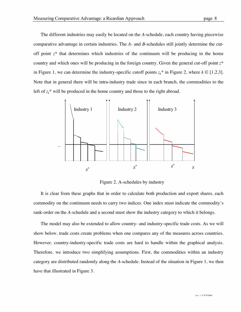
The different industries may easily be located on the A-schedule, each country having piecewise

comparative advantage in certain industries. The A- and B-schedules still jointly determine the cut-

off point z* that determines which industries of the continuum will be producing in the home

country and which ones will be producing in the foreign country. Given the general cut-off point z*

in Figure 1, we can determine the industry-specific cutoff points zk* in Figure 2, where k ∈ [1,2,3].

Note that in general there will be intra-industry trade since in each branch, the commodities to the

left of zk* will be produced in the home country and those to the right abroad.

Figure 2. A-schedules by industry

It is clear from these graphs that in order to calculate both production and export shares, each

commodity on the continuum needs to carry two indices. One index must indicate the commodity’s

rank-order on the A-schedule and a second must show the industry category to which it belongs.

The model may also be extended to allow country- and industry-specific trade costs. As we will

show below, trade costs create problems when one compares any of the measures across countries.

However, country-industry-specific trade costs are hard to handle within the graphical analysis.

Therefore, we introduce two simplifying assumptions. First, the commodities within an industry

category are distributed randomly along the A-schedule. Instead of the situation in Figure 1, we then

have that illustrated in Figure 3.

z

_

Industry 1

z*

Industry 2

z*

Industry 3

z*


jm / 12/3/06

Figure 3. Randomly distributed industries

Second, we assume that transport costs are uniform but specific to each industry.5 The first

assumption allows drawing up continuous schedules of relative unit production costs, as illustrated

by the solid downward-sloping curves in Figure 4. The second assumption allows adding

corresponding schedules of production plus transport costs for each country, as illustrated by the

dotted curves in the same figure. Within each industry, the dotted curve on the left shows the limit

to the goods that the home country can produce for export, while that on the right is the limit to

those that the foreign country can export. Between the two curves are the non-traded goods in each

industry.

5 This assumption is relaxed in the simulation analysis below.

_

A-schedule

z

B-schedule


jm / 12/3/06

Figure 4. Industry-specific transport costs

Combining our discussion with the graphs above, we summarize as follows: (1) In the DFS

model, both with and without transportation costs, production and exports are not perfectly

correlated, not even for all traded goods. A small country that exports a certain good does so

proportionally to the size of the rest of the world, while it imports proportionally to its own size.

However, production and export shares are perfectly correlated in the absence of trade costs, since

the relative size of a country does not matter for shares. (2) In the presence of transport costs, due to

the existence of non-traded goods within each industry, both measures are imperfect reflections of

actual comparative advantage. (3) The greater the asymmetries of transport costs across countries

and industries, the greater are the distortions that separate observed production and exports from the

underlying relative unit production costs. Eaton and Kortum (2002) have proposed a counterfactual

method that allows estimating trade flows in the absence of such transport-cost asymmetries.

However, their procedure cannot be easily applied to the non-traded goods within each industry.

_

Industry 1

z*

Industry 2

z*

Industry 3

zz*

Non-traded Goods


jm / 12/3/06

Next we derive these results formally in the context of the DFS (1977) model, which can be

skipped at a first read. Then we use counterfactuals to construct improved measures of comparative

advantage.

2.2 Technology

The world economy, consisting of two countries, produces consumer products which will be

indexed by i, i ∈ [1, N], where N indicates the total number of products that are either produced at

home or abroad. Any reader familiar with DFS (1977) can skip this and the next section, since I

merely replace the continuum of products in the DFS (1977) framework with discrete products.

Later on, I will additionally group the commodities into industries. For a given i, a(i) and a*(i) are

the home and foreign countries’ respective unit labor requirements. Each good can then be

characterized by its relative unit labor-requirement a*(i)/a(i). Home and foreign workers receive

wages w and w* determined by the condition that trade between the two countries be balanced.

In the absence of trade costs, the home country will produce a certain good i if it is the low-cost

producer:

** )()( wiawia ! . [1]

However, with trade costs the situation changes, since only a fraction of the goods produced will

survive iceberg trade costs. Let g(.) and g*(.) be the fractions of FOB value that survive after

shipment to their destination in the foreign and home country respectively. These costs can in

principle be country-pair or industry-specific and are assumed to be a function of distance, tariffs,

institutions and the like.6 However, in what follows we will assume that they are country specific

6 Since the use of tariff income is irrelevant for the question we address, we assume no redistribution of tariff income

as wages. For a detailed discussion of the effect of this redistribution, see DFS(1977).


jm / 12/3/06

for ease of exposition.7 Since there exist only two countries in our world, we index trade costs only

by the country of origin. The home country will therefore produce commodity i only as long as

(.)

)()(

*

**

g

wiawia ! [2]

Consider first the situation in which commodities are sorted by decreasing order of the home

country’s comparative advantage amended for trade costs. The relative comparative advantage of

the foreign country in the home country’s market can be characterized by the following discrete

function:

).()1(,)(

(.)/)()( **

***

iAiAia

giaiA <+! [3]

where we assume that the ratio A*(i) is unique for all i to simplify the solution of the model.

Similarly, exports from the home country will be too expensive and therefore the foreign country

will produce commodity i as long as

)(

)()( **

!"g

wiawia [4]

Consequently, the home country's comparative advantage adjusted for costs of trade can be

characterized by:

)()1(,)(/)(

)()(

*

iAiAgia

iaiA <+

!"

Without loss of generality, we assume that the costs of trade are determined by exporting

country factors like shipping and transaction technology. The home country produces a range of

commodities indexed from 1 to some borderline commodity ))(,( **!gz " , which is defined by:

( ) 1),( *1*** +<!"

zgAz # [5]

7 As mentioned earlier, in the simulation we allow g and g* to be also industry-specific. However, this only poses

complications in terms of indexing the products and therefore the graphical representation, since the ordering in terms of lowest production- and trade costs combined may vary across countries.


jm / 12/3/06

where )(1 !"A is the inverse function of )(iA and *

ww=! . The foreign country produces

commodities ranging from ),( gz ! to N with

( ) 1),(1

+<!"

zgAz # [6]

and z≤ z*.

This situation can be depicted as in Figure 5, where we approximate using continuous functions:

Figure 5. Transport costs

Equations [4] and [5] together with Figure 5 reveal that the home country's export performance

is jointly determined by the relative unit labor costs and trade costs of both countries. However, the

borderline good that the home country exports is determined by its own technological advantage

and trade cost. The borderline commodity, z, in which the home country has a comparative

production disadvantage but that it nevertheless produces is determined by the foreign country's

trade cost. For given technologies and trade costs, it follows that the relative wage has to fall within

the following interval:

Transport Costs

Produced in Foreign

Produced at Home

Non-Traded

z*z

_

A(i)

A*(i)

i


jm / 12/3/06

,)(

(.)*/)(

(.)/)(

)( **

ia

gia

gja

ja!!" i ≤ z*, j ≥ z. [7]

Adjusted for trade costs, the home country has a comparative advantage in all goods indexed i

on the right side of this inequality while the foreign country has a comparative advantage in the

goods indexed j on the left hand side of the inequality.

2.3 Demand

For simplicity, let us assume identical Cobb-Douglas preferences. Less restrictive assumptions

do not yield very different results as long as preferences are homothetic (Dornbusch et al., 1977,

826, n. 3). Cobb-Douglas preferences guarantee constant expenditure shares. Define b(i) as the

share of domestic income, Y, spent on good i:

iY

icipib !>= 0

)()()( , [8]

where c(i) is domestic consumption for commodity i and p(i) is its price. There is positive demand

for all goods. By definition,

1)(1

=!=

N

i

ib . [9]

Identical preferences in the two countries then guarantee that

)()( *ibib = . [10]

The share of foreign income Y* spent on imported goods is defined as

!=

=z

i

ib

1

)(" [11]


jm / 12/3/06

where z is the borderline good that is no longer exclusively produced in the home country and

),( g!"" = . The share of domestic income Y spent on goods produced in the foreign country is

therefore

!+=

=N

zi

ib

1*

* )(" , [12]

where z* denotes the hypothetical incremental commodity that is no longer produced at home and

),( ***g!"" = . The actual "borderline" commodities will be determined in equilibrium.

Equilibrium requires that domestic labor income equals world spending on domestically produced

goods:

( ) ***1 LwwLwL !+!"= ## [13]

where L and L* are the labor supplies in home and foreign respectively. [13] can be rewritten as:

!!"

#$$%

&'(=

L

LzzB

L

L*

**

*,,

)

)* [14]

since z and z* determine λ and λ*. The function B(.) characterizes the demand-side of the model. For

given relative labor endowments, it represents relative factor incomes ω that are consistent with

patterns of trade as determined by z and z*. It is increasing in the share of income foreigners spend

on goods produced at home and vice versa. Since all income is spend on commodities i in our

model, relative factor-incomes also determine relative demands for products, and B(.) is therefore

commonly referred to as the demand schedule.

Equilibrium is then characterized by:

)(;;)( ***

**

*zA

L

LzzB

L

LzA !""

#

$%%&

'=(=!

)

)* , [15]

where the bars over variables indicate their equilibrium values.


jm / 12/3/06

3. MEASURES OF COMPARATIVE ADVANTAGE

In this section, we first present theoretical measures of comparative advantage based on our

model. Then we derive commonly used empirical measures of comparative advantage from our

model. Finally we study how these relate to each other.

3.1 A Theoretically Correct Measure of Comparative Advantage

Relative unit production costs are unobservable in a world where all goods are traded and

production is completely specialized. Therefore, theoretical measures based on relative unit

production costs may be elegant, but empirical counterparts are nonexistent for traded goods. To

study the empirical performance of currently used empirical measures, we turn to a simpler

alternative that follows directly from the theory: A country has a comparative advantage in

producing a certain good if it is relatively better at producing this good than a competing country. It

is therefore evident that at the product level, comparative advantage can be represented by a binary

measure: a country either has a comparative advantage or it does not. In the absence of trade costs,

there is complete specialization at this level. At the industry level, such complete specialization is

not likely to be the case: some commodities within an industry may be produced in the home

country, some in the foreign country. Consequently a country may have a comparative advantage in

some but not all of the goods in an industry. A first approach to measure comparative advantage on

the industry level is therefore to simply count the number of goods within industry k that a country

produces, which I will call kn and *

kn for the home and foreign country respectively. However,

unless both countries are of the same size and industries are defined in a way that each one covers

the same number of products, this measure does not lend itself easily to comparisons across

industries and countries.

To allow for easier comparisons across countries, nk can be adjusted for country size. The

equivalent of country size is the number of commodities produced in a country, n and n*. If in


jm / 12/3/06

addition one controls for the number of commodities in an industry relative to all commodities in

the world, one obtains the formal equivalent of commodity counts to the Balassa-Index.

If there are positive trade costs an additional complication arises: namely, the presence of non-

traded goods. While it is still easy to determine which country has a comparative advantage at the

product level for traded goods, this distinction is not as simple for non-traded goods. Recall that

whether a country has comparative advantage in producing a good is determined by the

exogenously given relative technologies as well as the endogenously determined relative wage. The

relative wage is not only influenced by factor availability and technology, but also by trade costs

since they determine the share of non-traded goods.8 For any given relative wage, we can calculate

domestic prices for all non-traded goods in home and foreign markets. The home country has a

comparative advantage in producing those non-traded goods whose domestic price is lower than the

price in the foreign market. For all other non-traded goods, it has comparative disadvantage. Since

this cut-off point depends on the relative wage, it is clear that changes in transportation costs

influence the wage and may also change the set of non-traded commodities in which a country has a

comparative advantage.

To summarize, the model implies theoretically correct measures of comparative advantage. At

the product level, a country has a comparative advantage if it either exports the product or has a

lower domestic price. To find a comparable measure at the industry level, we count the number of

products in the industry in which a country has a comparative advantage. We can then adjust for

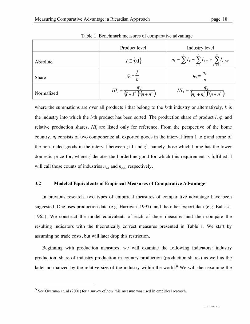
country and industry size. Table 1 displays these measures of comparative advantage based on our

model at the product and industry level.

8 Strictly speaking, we therefore can never exactly determine comparative advantage unless we know unit costs under

autarky. All we can do is therefore determine comparative advantage taking the relative wage as given, despite the fact that it is endogenously determined.


jm / 12/3/06

Table 1. Benchmark measures of comparative advantage

Product level Industry level

Absolute { }1,0!I !!!+===

+=='

1

,

1

,

1

z

zi

NTk

z

i

Tk

n

i

kkIIIn

Share n

I

i=!

n

nk

k=!

Normalized ( )( )**nnII

HIi

i

++=

! ( )( )**

nnnnHI

kk

k

k

++=

!

where the summations are over all products i that belong to the k-th industry or alternatively, k is

the industry into which the i-th product has been sorted. The production share of product i, φi and

relative production shares, HIi are listed only for reference. From the perspective of the home

country, nk consists of two components: all exported goods in the interval from 1 to z and some of

the non-traded goods in the interval between z+1 and z*, namely those which home has the lower

domestic price for, where z' denotes the borderline good for which this requirement is fulfilled. I

will call those counts of industries nk,T and nk,NT respectively.

3.2 Modeled Equivalents of Empirical Measures of Comparative Advantage

In previous research, two types of empirical measures of comparative advantage have been

suggested. One uses production data (e.g. Harrigan, 1997), and the other export data (e.g. Balassa,

1965). We construct the model equivalents of each of these measures and then compare the

resulting indicators with the theoretically correct measures presented in Table 1. We start by

assuming no trade costs, but will later drop this restriction.

Beginning with production measures, we will examine the following indicators: industry

production, share of industry production in country production (production shares) as well as the

latter normalized by the relative size of the industry within the world.9 We will then examine the

9 See Overman et. al (2001) for a survey of how this measure was used in empirical research.


jm / 12/3/06

following export-based measures of comparative advantage: industry exports, share of industry

exports in country exports (export shares), and the latter normalized by the share of industry exports

in world exports, commonly referred to as the Balassa Index. In the derivations that follow, we will

focus on the home country at the industry level.

As before, each commodity i will be sorted into an industry k. We therefore add industry indices

k. Then we analyze the relationship of the different measures of comparative advantage to one

other. We normalize world income to .1=wY Let the home country's share in world income be ! .

Consider first the commodity level. Define i

! as the home country's production of commodity i as

a fraction of world income (or production). )(ibi=! if i is a traded good and )(ib

i!="# if it is

non-traded. Now move up to the industry level. The home country's production of industry k as a

fraction of world income is NTkTk

z

i

z

z

kkkibib ,,

1 1

*

)()( !!!! +=+=" "= +

, where we have now added the

second index k to indicate that each good i belongs to an industry k. T and NT indicate traded and

non-traded goods respectively. Let the home country's share in world production overall be

!=

=M

k

k

1

"" , where M denotes the number of industries. Industry k's production as a share of total

home country production is then defined as: !!"kk

= . FOB exports of tradable commodity i are

)()1()( ibie !"= . Therefore, industry k’s exports are !=

"=z

i

kkibe

1

)()1( # . The home country’s total

exports (FOB) are !!!= ==

"==M

k

z

i

k

M

k

kibee

1 11

)()1( # and world exports are *eeew

+= . Finally, the

home country's exports in industry k as a share of the country’s total exports are eekk

=! . It

follows, that even with country-industry specific iceberg trade costs that Tn

Tk

k

,

,

!

!" = , since foreigners

pay the domestic price, but quantities are melted away, which leads them to pay an "implicit" higher

price. The other measures follow analogously. We can therefore summarize our measures on the

industry level before we move forward to compare them to one other:


jm / 12/3/06

Table 2. A comparison of modeled empirical measures of comparative advantage

Production Exports

Absolutea k! Tkk

e ,)1( !!"=

Share !

!" k

k=

Tn

Tkk

k

e

e

,

,

!

!" ==

Normalized *

kk

k

kHI

!!

"

+=

ww

k

k

ww

k

k

k

eeee

eeBI

!==

a with world income normalized to one, as in DFS (1977).

We are now ready to study how these measures compare to our theoretically correct measure and

how they are related to one other.

3.3 Comparisons between the Measures

In this section, we compare the empirical measures generated by the model with their theoretical

benchmarks. We do so by generating correlation coefficients between the benchmarks and

empirical measures by simulating the model numerically. While analytical solutions can be derived

for simple (e.g. uniform) trade costs, this is impossible for complex structures of trade costs, for

example when trade costs are industry-specific. The specific functional forms for technology, the

costs of trade as well as parameter values employed can be found in appendix A. We analyze

potential influences on the behavior of these measures, namely technological advantage, country

size, the number of industries, how evenly commodities are distributed across industries as well as

uniform and industry-specific trade costs. The results are presented in table 3 and 4 in appendix B.

The tables reveal three major results: (1) Production shares, export shares and relative production

shares are all perfectly correlated with their corresponding benchmark measures from table 1,

regardless of country size and relative technology level. (2) The Balassa-index is only correlated

with its theoretical equivalent when countries are of equal size and none of them has a technological


jm / 12/3/06

advantage on average. (3) All measures perform more or less poorly when trade costs are present.

There is no dominant measure that outperforms all others in all situations.

The first result is demonstrated in the first row of tables 3 and 4. It is what one should expect

based on the work by Harrigan (1997). Extending his argument to export shares is straightforward,

since normalizing a country's export in an industry with overall country exports eliminates the

influence of country-size. It is not as straightforward that the same holds for relative production

shares, but can be understood from the explanation of the second result.

The first row of quadrants in tables 3 and 4 also reveal that the Balassa-index (shaded in gray) is

not perfectly correlated with its theoretical benchmark unless the home and foreign country are of

the same size and there is no technological advantage on average for either country. This can be

explained by the following experiment: assume that a small country loses comparative advantage in

one good in a particular industry and gains comparative advantage in one good in another industry.

This only changes kn and *

kn , but not (

kn + *

kn ) in the corresponding measure in table 1. Therefore,

only the numerator of the measure in table 1 changes. However, in the Balassa-index, the numerator

and the denominator change simultaneously in both industries. This is due to the fact that the small

country exports proportionally to the rest of the world's size, while it imports proportionally to its

own size. Consequently, in the industry that loses one commodity from the small country's

perspective, world exports decline since the large exports from the small country to the rest of the

world are replaced with small exports from the rest of the world to the small country. The opposite

is true for the other industry involved. Consequently, the Balassa index cannot be perfectly

correlated with the measure based on industry counts. Technological advantage has a similar

influence, since an increase in average technological advantage increases the economic size of a

country and also makes exports and imports for the two countries asymmetric. Note, however, that

this only matters across industries, not within industries across countries. Consequently, the

Balassa-Index is still a valid measure of comparative advantage for a particular industry across

countries, since it is perfectly correlated with export shares across countries in any given industry


jm / 12/3/06

and year. But comparisons across industries and time do not reflect comparative advantage

accurately. However, the index by definition still measures relative export performance correctly,

even across industries and time, and this can still be a useful measure for country analysis. Since the

index of relative production shares is immune to these problems, it suggests itself for comparisons

across industries and countries as a means of comparison of comparative advantage.

The third result has to be taken with a grain of salt, since it likely is the one most specific to the

Ricardian model employed. However, the observations may be interesting enough to warrant more

general investigation. The third result can be seen by comparing corresponding rows in tables 3 and

4: when trade costs are present, the model does not deliver a "champion": There is no single

measure that consistently outperforms all others. But comparing corresponding columns in both

tables suggests directions for future research: it seems that relative production shares outperform all

other measures for small countries, or more precisely, when there are large asymmetries between

small and large countries and the research interest is on the small countries. Export shares perform

reasonably well when trade costs are not too "large". If the home country has a technological

advantage on average, then all measures tend to be more accurate even in the presence of trade

costs. All these effects are caused by the same driving force: whatever makes the analyzed country

resemble the world economy more closely increases the correlation between the empirical measures

and their theoretical counterparts (with exception, of course, of the Balassa-index). Consequently, a

larger country, higher relative technology and lower, more evenly distributed trade costs across

industries all tend to improve the accuracy of the measures. Finally, using a finer industry

classification tends to improve performance. Uneven distribution of commodities across industries

(implying relatively small and large industries) surprisingly doesn't seem to hurt, but rather to help

accuracy of the measures. While this may be due to simple aggregation effects, this needs to be

explored in more detail.

The results from this section suggest that the Balassa-index is inappropriate for analysis of

comparative advantage across industries. This seems to suggest employing production based


jm / 12/3/06

measures whenever available. However, if international trade costs could be accounted for, export-

based measures would be preferable at least for traded goods. We will suggest such a procedure

based on Eaton & Kortum (2002). We will also show that it is possible to obtain a general and

theoretically correct measure of comparative advantage from the Balassa-Index through regression

analysis. Combining the theoretically correct measure derived from the Balassa-Index with the

procedure that accounts for trade costs allows studying influences on comparative advantage and

costs of trade separately. We therefore derive estimation equations for the Balassa-Index next.

4. ESTIMATING MODELS OF COMPARATIVE ADVANTAGE AND RELATIVE EXPORT PERFORMANCE

Rewriting the expression for exports, solving it for c and inserting it back into the export

equation provides us with the following expression for exports:

( ) ( ))(

)1()()()1(

ip

iawibibie

k

kk

!!

"###="#= [16]

Inserting [16] back into the formula for the Balassa-Index and simplifying leads to:

!!"

#$$%

&''+'('!!

"

#$$%

&''+'('

=

) )))))

)))

= +== =+==

= ==

M

k

N

zi k

kM

k

z

i k

kN

zi k

kz

i k

k

M

k

z

i k

kz

i k

k

k

ip

iaw

ip

iaw

ip

iaw

ip

iaw

ip

ia

ip

ia

BI

1 1*

*

*

1 11*

*

*

1

1 11

** )(

)(

)(

)()1(

)(

)(

)(

)()1(

)(

)(

)(

)(

****

[17]

If all the required data is available, [17] can be estimated directly by taking logs on both sides.

Simplifying this expression, however, [17] can be rewritten as:

( )( )** )1()1( !"!"#"#"

!#

$+$%$+$%=

kk

k

kBI [18]

where k

! is the share of industry k in all commodities that fall into the interval from 1 to z, and *

k! is the share of industry k in all commodities that fall into the interval from z* + 1 to N. Taking

logs on both sides, we obtain:


jm / 12/3/06

( ) ( )** )1(ln)1(ln)ln()ln()ln( !"!"#"#"!# $+$%+$+$%%%=kkkk

BI [19]

Estimating [19] reveals that under the assumption that the data is generated by a ricardian model

as specified above, in a regression of the Balassa-Index on a constant, country- and industry

dummies the error term ε of this regression provides a measure proportional to the number of

products a country produces in industry k.

!""# +++=ICkDDBI 11)ln( [20]

It follows from [17] that kk eip

ia+!!"

#$$%

&=

)(

)(ln0'( , and from the Frish-Waugh-Lovell-Theorem that

[20] can therefore be written in the following form,

!"""# +++$$%

&''(

)+= ICk DD

ip

iaBI 210

)(

)(ln)ln( [21]

where the second term is proportional to ln(σk) again. Consequently, [21] can be used to

estimate influences on comparative advantage directly, despite the fact that the Balassa-Index itself

is generally not a valid measure of comparative advantage. We will provide an example of this in

section 5.3 of the paper. Alternatively, of course, it is also valid to use the following estimation to

obtain identical results:

!""#$ ++%%&

'(()

*+= Ck D

ip

ia10

)(

)(ln)ln( [22]

where we replaced the left hand side with export shares. The definition of exports [16] can also

be estimated. Its simple structure is identical to a very simple version of the gravity model in

empirical trade. Since industry-specific factors on the right hand side are the main drivers of exports

in this model, while all other influences are absorbed in dummy-variables, one can interpret the

estimation technique that results from our theoretical model as an amended version of the gravity

equation. In fact, Feenstra (2004) has suggested using country-specific dummy-variables to replace

the multilateral resistance terms derived in Anderson and van Wincoop (2004). We find similar

terms in our regression. However, since our analysis is industry-specific, country- and industry


jm / 12/3/06

specific price-terms have to be included in the regression in order to avoid omitted variable bias. In

principle, the framework above can easily be adapted to bilateral aspects of comparative advantage

based on the work of Eaton and Kortum (2002) and Deardorff (2004b). Finally, the above analysis

suggests that the original specification of Balassa (1965) was invalid.

5. DISENTANGLING COMPARATIVE ADVANTAGE AND COSTS OF TRADE

While the assumption of iceberg transportation costs is technically elegant, it does not reflect

the actual organization of transactions. The specification above harbors a major problem: FOB

exports are not equivalent to the true value purchased by foreigners before melting, they are the true

value equivalent before adding costs of international trade. I introduce a simple version of this next.

5.1 Trade Costs as Mark-Ups

I keep the simple assumptions about preferences but change the notation such that trade costs

are a country-pair and industry-specific markup over regular FOB values. Consequently, the FOB

export data we observe is )()()( *icipie

o!= . The survival fraction gk(i) of the previous sections is

simply the inverse of the markup, therefore:

( )

( ) )1()()(

)(

)(

*,!"#=#= ibic

ig

ip

ig

ie

kk

ok [23]

Under the assumption that a solution for the relative wage and the relative prices exist, [23] can

be written as:

( ) ( ))(

)()1()()()()1(,

ip

igiawibigibie kk

kok

!"!!!=!"!=

## [24]

Implementing this into the Balassa-Index yields in its simplest version:


jm / 12/3/06

!!"

#$$%

&'+'(!!

"

#$$%

&'+'(

=

) )))))

)))

= +== =+==

= ==

M

k

N

zi

k

M

k

z

i

k

N

zi

k

z

i

k

M

k

z

i

k

z

i

k

gk

igigigig

igig

BI

1 1

*

1 11

*

1

1 11

,

**

)()()1()()()1(

)()(

****

[25]

This expression cannot be simplified if gk (i) are country-pair and industry-specific. However,

several cases are possible in which the above expression can be simplified, for example if

gigig kk == )()( * , then BIk,g = BIk. Generally, however, we can implicitly define

GBIBI kgk !=,

,

where G = f(gk (i)) is a scaling factor which is a function of the trade costs for each commodity.

From the expression above, it is hard to solve for G analytically. However, G can be approximated

using a statistical method proposed by Eaton and Kortum (2002). We turn to this procedure next.

5.2 Counterfactual Estimates

Recall from above that observable exports can be written as:

( ) ( ) )()1(, igibie kok !"!= # [26]

Taking logs on both sides, this can be written as the following estimation equation:

( )( ) ( )( ) ( ) ( ) !" ++#+= )(ln1lnlnln , igibie kok

In order to estimate this model, we will make the following identifying assumption: gk(i) is

assumed to be country-pair specific in the sense that it is a function of distance and the country of

origin. We therefore actually estimate the following model:

( )( ) !"##$ ++++= hfhffhihifh dDDie ,ln [27]

where h, f indicate the home and the foreign country respectively, Dhi is a dummy variable that

assumes the value 1 for country h and industry i and zero otherwise, Df is a dummy variable that

assumes the value 1 for country f and zero otherwise, and dhf is the distance between the two

countries. We then construct counterfactuals as in Eaton and Kortum(2002), where we calculate )(ˆ iehf for the case of zero distance between the two countries. These estimates are then again used


jm / 12/3/06

to construct export-based measures of comparative advantage. In particular, we will calculate the

Balassa-Index for zero trade costs, BIk0. We will use this index to recover the trade-cost index

0kkBIBIG = . BIk0 and G can be used to study influences that may affect comparative advantage

(new technology), the costs of trade (length of the coastline, number of ports) or both (institutions).

For our demonstration exercise, I only use three widely used industry-categories suggested in

Rauch(1999): He sorted four digit SITC industries into those that are traded on organized

exchanges, those that are reference priced and those that are neither. In recent work (Berkowitz et.

al. 2004), the first and the last category are referred to as simple and complex goods respectively.

Complex vs. Simple

Simple Complex

Eaton and Kortum (2002) demonstrated how to estimate this ricardian model in a multi-country

setting. In order to get more reliable results, we therefore estimate bilateral trade relationships and

construct counterfactuals for the 55 countries listed in table 5 in appendix B for the years 1982 and

1992. Trade data comes from the World Trade Database of Statistics Canada. Bilateral distances are

the same as in Rauch (1999). For those three industry categories, we plot the relationship between

BIk and BIk0, which are labeled RCA and CA respectively in the following graphs. Each point

represents a country.


jm / 12/3/06

BIk and BIk0 for goods traded on organized exchanges in 1982 (left panel) and 1992 (right panel)

BIk and BIk0 for reference priced goods in 1982 (left panel) and 1992 (right panel)

BIk and BIk0 for goods that fall in neither category in 1982 (left panel) and 1992 (right panel)


jm / 12/3/06

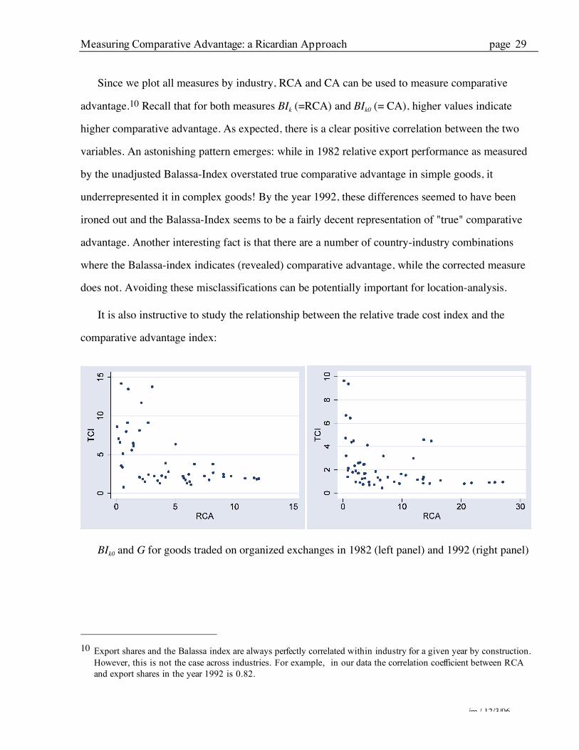
Since we plot all measures by industry, RCA and CA can be used to measure comparative

advantage.10 Recall that for both measures BIk (=RCA) and BIk0 (= CA), higher values indicate

higher comparative advantage. As expected, there is a clear positive correlation between the two

variables. An astonishing pattern emerges: while in 1982 relative export performance as measured

by the unadjusted Balassa-Index overstated true comparative advantage in simple goods, it

underrepresented it in complex goods! By the year 1992, these differences seemed to have been

ironed out and the Balassa-Index seems to be a fairly decent representation of "true" comparative

advantage. Another interesting fact is that there are a number of country-industry combinations

where the Balassa-index indicates (revealed) comparative advantage, while the corrected measure

does not. Avoiding these misclassifications can be potentially important for location-analysis.

It is also instructive to study the relationship between the relative trade cost index and the

comparative advantage index:

BIk0 and G for goods traded on organized exchanges in 1982 (left panel) and 1992 (right panel)

10 Export shares and the Balassa index are always perfectly correlated within industry for a given year by construction.

However, this is not the case across industries. For example, in our data the correlation coefficient between RCA and export shares in the year 1992 is 0.82.


jm / 12/3/06

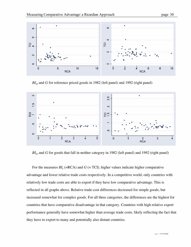
BIk0 and G for reference priced goods in 1982 (left panel) and 1992 (right panel)

BIk0 and G for goods that fall in neither category in 1982 (left panel) and 1992 (right panel)

For the measures BIk (=RCA) and G (= TCI), higher values indicate higher comparative

advantage and lower relative trade costs respectively. In a competitive world, only countries with

relatively low trade costs are able to export if they have low comparative advantage. This is

reflected in all graphs above. Relative trade-cost differences decreased for simple goods, but

increased somewhat for complex goods. For all three categories, the differences are the highest for

countries that have comparative disadvantage in that category. Countries with high relative export

performance generally have somewhat higher than average trade costs, likely reflecting the fact that

they have to export to many and potentially also distant countries.


jm / 12/3/06

In the next section, we will use these measures as left-hand side variables in order to estimate

influences on comparative advantage and costs of trade jointly.

5.3 Estimating Influences on Comparative Advantage and the Costs of Trade

The two indices derived above, BIk0 and G, can now be used to study influences on comparative

advantage and relative costs of trade. The regression equations are analogous to the ones in [21]:

!"""# +++$$%

&''(

)+= ICk DD

ip

iaBI 2100

)(

)(ln)ln( [28]

( ) !"""# ++++= ICk DDigG 2100 )(ln)ln( [29]

Note that industry-dummies are included on the right hand side, which allows us to include all

industries in the sample. As a simple example, researchers have postulated that remoteness of a

country affects its trade, where remoteness is measured as GDP-weighted bilateral distances (Wei

1996). Remoteness should not affect technology, but should affect the prices charged, since firms in

a remote location are somewhat shielded from competition. It should also influence relative trade

costs, since long-hauls cost less per unit of distance than short hauls of freight. With the framework

developed here, we can estimate those effects directly. We do so for Balassa's relative export

performance as well as the two new measures developed in this paper. Since we only have one

parameter of interest, we only include this parameter for simplicity.11 The coefficient states the

differential effect of remoteness on complex versus simple goods. It indicates the percentage

change in the left-hand side measure given a one percent increase in the remoteness measure

relative to the other goods categories. We do the estimation for all years combined12 as well as the

beginning and the end of the sample period. The results are presented in the following table:

11 Recall from above that the derived specification requires price-data, which was not available to us for all countries.

Unfortunately, this implies that the presented results are likely biased due to omitted variable bias. However, since these regressions only serve illustrative purposes, we are not concerned about this issue here.

12 This requires to replace the industry dummies in [28] and [29] with industry-year dummies.


jm / 12/3/06

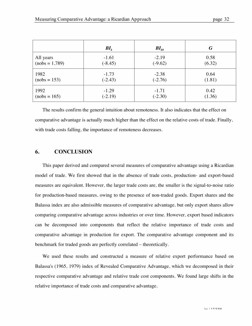
BIk BIk0 G

All years (nobs = 1,789)

-1.61 (-8.45)

-2.19 (-9.62)

0.58 (6.32)

1982 (nobs = 153)

-1.73 (-2.43)

-2.38 (-2.76)

0.64 (1.81)

1992 (nobs = 165)

-1.29 (-2.19)

-1.71 (-2.30)

0.42 (1.36)

The results confirm the general intuition about remoteness. It also indicates that the effect on

comparative advantage is actually much higher than the effect on the relative costs of trade. Finally,

with trade costs falling, the importance of remoteness decreases.

6. CONCLUSION

This paper derived and compared several measures of comparative advantage using a Ricardian

model of trade. We first showed that in the absence of trade costs, production- and export-based

measures are equivalent. However, the larger trade costs are, the smaller is the signal-to-noise ratio

for production-based measures, owing to the presence of non-traded goods. Export shares and the

Balassa index are also admissible measures of comparative advantage, but only export shares allow

comparing comparative advantage across industries or over time. However, export based indicators

can be decomposed into components that reflect the relative importance of trade costs and

comparative advantage in production for export. The comparative advantage component and its

benchmark for traded goods are perfectly correlated – theoretically.

We used these results and constructed a measure of relative export performance based on

Balassa's (1965, 1979) index of Revealed Comparative Advantage, which we decomposed in their

respective comparative advantage and relative trade cost components. We found large shifts in the

relative importance of trade costs and comparative advantage.


jm / 12/3/06

Finally, we used the two indices obtained from our decomposition of the Balassa Index to

demonstrate that both comparative advantage and costs of trade are affected by remoteness.

APPENDIX A: MODEL PARAMETERS

Number of products : 1000 Labor endowments: world 1000, distributed across home and foreign. Home share for small country = 0.1, home share for lage country = 0.9.

)1,0(21)( UAiah!!+= , where Ah denotes an average technology scale parameter and U(0,1) is the

uniform distribution between 0 and 1. The function for a*(i) is defined analogously.

( )( ))1,0(111 UtTg w

h!+!+= , where Th refers to the average trade cost factor at home, tw is a

redistribution weight generating increasing differences of trade costs across industries and is calculated for the kth industry as ( )Kkt

w!= " , where τ is a scalar and K is the total number of

industries. The function for g* is defined analogously. Th = 0.1 for low uniform trade costs and Th = 3 for high trade costs. τ = 0.1 for small trade cost differences across industries and 3 for large ones.

Number of industries: small = 10, large = 100.

Scaling factor for distribution of industries: even distribution = 1, uneven distribution = 3 Technology Ah = 1, home advantage Ah = 5. Runs per average correlation: 100

Date post:	06-Mar-2018
Category:	Documents
Upload:	phungdung
View:	240 times
Download:	3 times

Measuring Comparative Advantage: A Ricardian · PDF fileMeasuring Comparative Advantage: a...

Documents