255
Measuring Inequality Frank A. Cowell December 2009 http://darp.lse.ac.uk/MI3
Measuring Inequality
Frank A. Cowell
December 2009http://darp.lse.ac.uk/MI3
ii
Abstract
� Part of the series LSE Perspectives in Economic Analysis, pub-lished by Oxford University Press
� This book is dedicated to the memory of my parents.
Contents
Preface xi
1 First Principles 11.1 A preview of the book . . . . . . . . . . . . . . . . . . . . . . . . 31.2 Inequality of what? . . . . . . . . . . . . . . . . . . . . . . . . . . 41.3 Inequality measurement, justice and poverty . . . . . . . . . . . . 71.4 Inequality and the social structure . . . . . . . . . . . . . . . . . 121.5 Questions . . . . . . . . . . . . . . . . . . . . . . . . . . . . . . . 13
2 Charting Inequality 172.1 Diagrams . . . . . . . . . . . . . . . . . . . . . . . . . . . . . . . 172.2 Inequality measures . . . . . . . . . . . . . . . . . . . . . . . . . 232.3 Rankings . . . . . . . . . . . . . . . . . . . . . . . . . . . . . . . 302.4 From charts to analysis . . . . . . . . . . . . . . . . . . . . . . . 362.5 Questions . . . . . . . . . . . . . . . . . . . . . . . . . . . . . . . 36
3 Analysing Inequality 393.1 Social-welfare functions . . . . . . . . . . . . . . . . . . . . . . . 403.2 SWF-based inequality measures . . . . . . . . . . . . . . . . . . . 483.3 Inequality and information theory . . . . . . . . . . . . . . . . . 523.4 Building an inequality measure . . . . . . . . . . . . . . . . . . . 603.5 Choosing an inequality measure . . . . . . . . . . . . . . . . . . . 653.6 Summary . . . . . . . . . . . . . . . . . . . . . . . . . . . . . . . 703.7 Questions . . . . . . . . . . . . . . . . . . . . . . . . . . . . . . . 71
4 Modelling Inequality 754.1 The idea of a model . . . . . . . . . . . . . . . . . . . . . . . . . 764.2 The lognormal distribution . . . . . . . . . . . . . . . . . . . . . 774.3 The Pareto distribution . . . . . . . . . . . . . . . . . . . . . . . 844.4 How good are the functional forms? . . . . . . . . . . . . . . . . 914.5 Questions . . . . . . . . . . . . . . . . . . . . . . . . . . . . . . . 95
iii
iv CONTENTS
5 From Theory to Practice 995.1 The data . . . . . . . . . . . . . . . . . . . . . . . . . . . . . . . 1005.2 Computation of the inequality measures . . . . . . . . . . . . . . 1085.3 Appraising the calculations . . . . . . . . . . . . . . . . . . . . . 1245.4 Shortcuts: �tting functional forms1 . . . . . . . . . . . . . . . . . 1315.5 Interpreting the answers . . . . . . . . . . . . . . . . . . . . . . . 1385.6 A sort of conclusion . . . . . . . . . . . . . . . . . . . . . . . . . 1435.7 Questions . . . . . . . . . . . . . . . . . . . . . . . . . . . . . . . 144
A Technical Appendix 149A.1 Overview . . . . . . . . . . . . . . . . . . . . . . . . . . . . . . . 149A.2 Measures and their properties . . . . . . . . . . . . . . . . . . . . 149A.3 Functional forms of distribution . . . . . . . . . . . . . . . . . . . 152A.4 Interrelationships between inequality measures . . . . . . . . . . 160A.5 Decomposition of inequality measures . . . . . . . . . . . . . . . 161A.6 Negative incomes . . . . . . . . . . . . . . . . . . . . . . . . . . . 166A.7 Estimation problems . . . . . . . . . . . . . . . . . . . . . . . . . 168A.8 Using the website . . . . . . . . . . . . . . . . . . . . . . . . . . . 174
B Notes on Sources and Literature 177B.1 Chapter 1 . . . . . . . . . . . . . . . . . . . . . . . . . . . . . . . 177B.2 Chapter 2 . . . . . . . . . . . . . . . . . . . . . . . . . . . . . . . 179B.3 Chapter 3 . . . . . . . . . . . . . . . . . . . . . . . . . . . . . . . 182B.4 Chapter 4 . . . . . . . . . . . . . . . . . . . . . . . . . . . . . . . 186B.5 Chapter 5 . . . . . . . . . . . . . . . . . . . . . . . . . . . . . . . 190B.6 Technical Appendix . . . . . . . . . . . . . . . . . . . . . . . . . 195
1This section contains material of a more technical nature which can be omitted withoutloss of continuity.
List of Tables
1.1 Four inequality scales . . . . . . . . . . . . . . . . . . . . . . . . 9
3.1 How much should R give up to �nance a £ 1 bonus for P? . . . . 433.2 Is P further from Q than Q is from R? . . . . . . . . . . . . . . . 593.3 The break-down of inequality: poor East, rich West . . . . . . . 633.4 The break-down of inequality: the East catches up . . . . . . . . 643.5 Which measure does what? . . . . . . . . . . . . . . . . . . . . . 72
4.1 Pareto�s � and �average/base�inequality . . . . . . . . . . . . . 884.2 Pareto�s � for income distribution in the UK and the USA . . . . 94
5.1 Distribution of Income Before Tax. USA 2006. Source: InternalRevenue Service . . . . . . . . . . . . . . . . . . . . . . . . . . . . 112
5.2 Values of Inequality indices under a variety of assumptions aboutthe data. US 2006 . . . . . . . . . . . . . . . . . . . . . . . . . . 118
5.3 Approximation Formulas for Standard Errors of Inequality Mea-sures . . . . . . . . . . . . . . . . . . . . . . . . . . . . . . . . . . 126
5.4 Atkinson index and coe¢ cient of variation: IRS 1987 to 2006 . . 1285.5 Individual distribution of household net per capita annual in-
come. Czechoslovakia 1988. Source: see Appendix B . . . . . . . 1295.6 Average income, taxes and bene�ts by decile groups of all house-
holds. UK 1998-9. Source: O¢ ce for National Statistics . . . . . 1455.7 Observed and expected frequencies of household income per head,
Jiangsu, China . . . . . . . . . . . . . . . . . . . . . . . . . . . . 147
A.1 Inequality measures for discrete distributions . . . . . . . . . . . 151A.2 Inequality measures for continuous distributions . . . . . . . . . . 153A.3 Decomposition of inequality in Chinese provinces, Rural and Ur-
ban subpopulations . . . . . . . . . . . . . . . . . . . . . . . . . . 165A.4 Source �les for tables and �gures . . . . . . . . . . . . . . . . . . 175
v

vi LIST OF TABLES
List of Figures
1.1 Two Types of Inequality . . . . . . . . . . . . . . . . . . . . . . . 81.2 An Inequality Ranking . . . . . . . . . . . . . . . . . . . . . . . . 81.3 Alternative policies for Fantasia . . . . . . . . . . . . . . . . . . . 15
2.1 The Parade of Dwarfs. UK Income Before Tax, 1984/5. Source:Economic Trends, November 1987 . . . . . . . . . . . . . . . . . . . 19
2.2 Frequency Distribution of Income Source: as for Figure 2.1 . . . . 202.3 Cumulative Frequency Distribution. Source: as for Figure 2.1 . . . 212.4 Lorenz Curve of Income. Source: as for Figure 2.1 . . . . . . . . . 222.5 Frequency Distribution of Income (Logarithmic Scale).Source: as
for Figure 2.1 . . . . . . . . . . . . . . . . . . . . . . . . . . . . . . 232.6 The Parade with Partial Equalisation . . . . . . . . . . . . . . . 252.7 The High-Low Approach . . . . . . . . . . . . . . . . . . . . . . . 282.8 The Parade and the Quantile Ranking . . . . . . . . . . . . . . . 312.9 Quantile ratios of earnings of adult men, UK 1968-2007. Source:
Annual Survey of Hours and Earnings . . . . . . . . . . . . . . . . . 322.10 Ranking by Shares. UK 1984/5 Incomes before and after tax.
Source: as for Figure 2.1 . . . . . . . . . . . . . . . . . . . . . . . . 332.11 Lorenz Curves Crossing . . . . . . . . . . . . . . . . . . . . . . . 342.12 Change at the bottom of the income distribution . . . . . . . . . 352.13 Change at the top of the income distribution . . . . . . . . . . . 35
3.1 Social utility and relative income . . . . . . . . . . . . . . . . . . 443.2 The relationship between welfare weight and income. . . . . . . . 453.3 The Generalised Lorenz Curve Comparison: UK income before
tax . . . . . . . . . . . . . . . . . . . . . . . . . . . . . . . . . . . 473.4 Distribution of Income and Distribution of Social Utility . . . . . 493.5 The Atkinson and Dalton Indices . . . . . . . . . . . . . . . . . . 503.6 The Theil Curve . . . . . . . . . . . . . . . . . . . . . . . . . . . 543.7 Theil�s Entropy Index . . . . . . . . . . . . . . . . . . . . . . . . 563.8 A variety of distance concepts . . . . . . . . . . . . . . . . . . . . 583.9 Lorenz Curves for Equivalised Disposable Income per Person.
Switzerland and USA. . . . . . . . . . . . . . . . . . . . . . . . . 69
vii
viii LIST OF FIGURES
3.10 Inequality Aversion and Inequality Rankings, Switzerland andUSA. Source: as for Figure 3.9 . . . . . . . . . . . . . . . . . . . . 70
4.1 The Normal Distribution . . . . . . . . . . . . . . . . . . . . . . . 784.2 The Lognormal Distribution . . . . . . . . . . . . . . . . . . . . 794.3 The Lorenz curve for the Lognormal distribution . . . . . . . . . 814.4 Inequality and the Lognormal parameter �2 . . . . . . . . . . . . 824.5 The Pareto Diagram.Source: as for Figure 2.1 . . . . . . . . . . . . 854.6 The Pareto Distribution in the Pareto Diagram . . . . . . . . . . 864.7 Paretian frequency distribution . . . . . . . . . . . . . . . . . . . 874.8 The Lorenz curve for the Pareto distribution . . . . . . . . . . . 894.9 Inequality and Pareto�s � . . . . . . . . . . . . . . . . . . . . . . 904.10 The Distribution of Earnings. UK Male Manual Workers on Full-
Time Adult Rates. Source: New Earnings Survey, 2002 . . . . . . . 924.11 Pareto Diagram. UK Wealth Distribution 2003. Source: Inland
Revenue Statistics . . . . . . . . . . . . . . . . . . . . . . . . . . . 934.12 Pareto�s �: USA and UK. Source: see text . . . . . . . . . . . . . 95
5.1 Frequency Distribution of Income, UK 2005/6, Before and AfterTax. Source: Inland Revenue Statistics . . . . . . . . . . . . . . . . 101
5.2 Disposable Income (Before Housing Costs). UK 2006/7. Source:Households Below Average Income, 2008 . . . . . . . . . . . . . . 103
5.3 Disposable Income (After Housing Costs). UK 2006/7. Source:Households Below Average Income, 2008 . . . . . . . . . . . . . . 104
5.4 Income Observations Arranged on a Line . . . . . . . . . . . . . 1105.5 Frequency Distribution of Disposable Income, UK 2006/7 (After
Housing Costs), Unsmoothed. Source: as for Figure 5.3 . . . . . 1115.6 Estimates of Distribution Function. Disposable Income, UK 2006/7.
(After Housing Costs), Moderate Smoothing. Source: as for Fig-ure 5.3 . . . . . . . . . . . . . . . . . . . . . . . . . . . . . . . . . 113
5.7 Estimates of Distribution Function. Disposable Income, UK 2006/7.(After Housing Costs), High Smoothing. Source: as for Figure 5.3 114
5.8 Frequency distribution of income before tax. US 2006. Source:Internal Revenue Service . . . . . . . . . . . . . . . . . . . . . . . . 115
5.9 Lower Bound Inequality, Distribution of Income Before Tax. US2006. Source: Internal Revenue Service . . . . . . . . . . . . . . . . 116
5.10 Upper Bound Inequality, Distribution of Income Before Tax. US2006. Source: Internal Revenue Service . . . . . . . . . . . . . . . . 117
5.11 The coe¢ cient of variation and the upper bound of the top interval.1205.12 Lorenz Co-ordinates for Table 5.1 . . . . . . . . . . . . . . . . . . 1215.13 Upper and Lower Bound Lorenz Curves . . . . . . . . . . . . . . 1225.14 The �split histogram�compromise. . . . . . . . . . . . . . . . . . 1245.15 Lorenz Curves �Income Before Tax. USA 1987 and 2006. Source:
Internal Revenue Service . . . . . . . . . . . . . . . . . . . . . . . . 1275.16 The Atkinson index for grouped data, US 2006. Source: as for
Table 5.1. . . . . . . . . . . . . . . . . . . . . . . . . . . . . . . . 128
LIST OF FIGURES ix
5.17 The Atkinson Index for Grouped Data: First interval deleted.Czechoslovakia 1988 . . . . . . . . . . . . . . . . . . . . . . . . . 130
5.18 The Atkinson Index for Grouped Data: All data included. Czechoslo-vakia 1988 . . . . . . . . . . . . . . . . . . . . . . . . . . . . . . . 131
5.19 Fitting the Pareto diagram for the data in Table 5.1 . . . . . . . 1365.20 Fitting the Pareto diagram for IRS data in 1987 (values in 2006
dollars) . . . . . . . . . . . . . . . . . . . . . . . . . . . . . . . . 1375.21 The minimum income growth to o¤set a 1% growth in inequality 140
A.1 Relationships Between Functional Forms . . . . . . . . . . . . . . 159A.2 Density Estimation with a Normal Kernel . . . . . . . . . . . . . 171

x LIST OF FIGURES
Preface
�It is not the business of the botanist to eradicate the weeds.Enough for him if he can tell us just how fast they grow.� � C.Northcote Parkinson (1958), Parkinson�s Law
The maligned botanist has a good deal to be said for him in the company ofrival gardeners, each propagating his own idea about the extent and the growthof thorns and thistles in the herbaceous border, and each with a patent weed-killer. I hope that this book will perform a similar role in the social scientist�stoolshed. It does not deal with theories of the development of income distribu-tion, of the generation of inequality, or of other social weeds, nor does it supplyany social herbicides. However, it does give a guide to some of the theoreticaland practical problems involved in an analysis of the extent of inequality thuspermitting an evaluation of the diverse approaches hitherto adopted. In avoidingpatent remedies for particular unwanted growths, one �nds 6useful analogies invarious related �elds �for example, some techniques for measuring economic in-equality have important counterparts in sociological and political studies. Thus,although I have written this as an economist, I would like to think that studentsin these related disciplines will be interested in this material.This book is deliberately limited in what it tries to do as far as expounding
theory, examining empirical evidence, or reviewing the burgeoning literature isconcerned. For this reason, a set of notes for each chapter is provided on pages177 ¤. The idea is that if you have not already been put o¤ the subject by thetext, then you can follow up technical and esoteric points in these notes, andalso �nd a guide to further reading.A satisfactory discussion of the techniques of inequality measurement in-
evitably involves the use of some mathematics. However, I hope that peoplewho are allergic to symbols will nevertheless read on. If you are allergic, youmay need to toil a little more heavily round the diagrams that are used fairlyextensively in Chapters 2 and 3. In fact the most sophisticated piece of notationwhich it is essential that all should understand in order to read the main bodyof the text is the expression
nXi=1
xi;
xi
xii PREFACE
representing the sum of n numbers indexed by the subscript i, thus: x1 + x2 +x3 + :::+ xn. Also it is helpful if the reader understands di¤erentiation, thoughthis is not strictly essential. Those who are happy with mathematical notationmay wish to refer directly to Appendix A in which formal de�nitions are listed,and where proofs of some of the assertions in the text are given. AppendixA also serves as a glossary of symbols used for inequality measures and otherexpressions.Associated with this book there is a website with links to data sources, down-
loadable spreadsheets of constructed datasets and examples and presentation�les showing the step-by-step developments of some arguments and techniques.Although you should be able to read the text without having to use the website,I am �rmly of the opinion that many of the issues in inequality measurementcan only be properly understood through experience with practical examples.There are quite a few numerical examples included in the text and several morewithin the questions and problems at the end of each chapter: you may well�nd that the easiest course is to pick up the data for these straight from thewebsite rather than doing them by hand or keying the numbers into a computeryourself. This is described further in the Appendix A (page 174), but to getgoing with the data you only go to the welcome page of the website.This book is in fact the third edition of a project that started a long time
ago. So I have many years�worth of intellectual debt that I would like to breakup into three tranches:
Acknowledgements from the �rst edition
I would like to thank Professor M. Bronfenbrenner for the use of the tableon page 94. The number of colleagues and students who wilfully submittedthemselves to reading drafts of this book was most gratifying. So I am verythankful for the comments of Tony Atkinson, Barbara Barker, John Bridge,David Collard, Shirley Dex, Les Fishman, Peter Hart, Kiyoshi Kuga, H. F.Lydall, M. D. McGrath, Neville Norman and Richard Ross; without them therewould have been lots more mistakes. You, the reader, owe a special debt toMike Harrison, John Proops and Mike Pullen who persistently made me makethe text more intelligible. Finally, I am extremely grateful for the skill andpatience of Sylvia Beech, Stephanie Cooper and Judy Gill, each of whom hashad a hand in producing the text; �so careful of the type she seems,�as Tennysononce put it.
Acknowledgements from the second edition
In preparing the second edition I received a lot of useful advice and help, par-ticularly from past and present colleagues in STICERD. Special thanks go toTony Atkinson, Karen Gardiner, John Hills, Stephen Jenkins, Peter Lambert,John Micklewright and Richard Vaughan for their comments on the redraftedchapters. Z. M. Kmietowicz kindly gave permission for the use of his recentwork in question 8 on page 146. Christian Schlüter helped greatly with the up-
xiii
dating the literature notes and references. Also warm appreciation to ElisabethBacker and Jumana Saleheen without whose unfailing assistance the revisionwould have been completed in half the time.
Acknowledgments for the present edition
I am very grateful for extended discussions with and support from GuillermoCruces and for detailed comments from Kristof Bosmans, Udo Ebert, MarcFleurbaey, Wulf Gaertner, Stephen Jenkins and Dirk Van de gaer. For much-needed help in updating the bibliography and data souces my thanks go toYinfei Dong, Elena Pisano, Alex Teytelboym and Zhijun Zhang.
STICERD, LSE

xiv PREFACE
Chapter 1
First Principles
�It is better to ask some of the questions than to know all ofthe answers.� �James Thurber (1945), The Scotty Who Knew TooMuch
�Inequality�is in itself an awkward word, as well as one used in connectionwith a number of awkward social and economic problems. The di¢ culty is thatthe word can trigger quite a number of di¤erent ideas in the mind of a readeror listener, depending on his training and prejudice.�Inequality�obviously suggests a departure from some idea of equality. This
may be nothing more than an unemotive mathematical statement, in which case�equality�just represents the fact that two or more given quantities are the samesize, and �inequality�merely relates to di¤erences in these quantities. On theother hand, the term �equality�evidently has compelling social overtones as astandard which it is presumably feasible for society to attain. The meaning tobe attached to this is not self-explanatory. Some years ago Professors Rein andMiller revealingly interpreted this standard of equality in nine separate ways
� One-hundred-percentism: in other words, complete horizontal equity ��equal treatment of equals.�
� The social minimum: here one aims to ensure that no one falls below someminimum standard of well-being.
� Equalisation of lifetime income pro�les: this focuses on inequality of futureincome prospects, rather than on the people�s current position.
� Mobility : that is, a desire to narrow the di¤erentials and to reduce thebarriers between occupational groups.
� Economic inclusion: the objective is to reduce or eliminate the feelingof exclusion from society caused by di¤erences in incomes or some otherendowment.
1
2 CHAPTER 1. FIRST PRINCIPLES
� Income shares: society aims to increase the share of national income (orsome other �cake�) enjoyed by a relatively disadvantaged group �such asthe lowest tenth of income recipients.
� Lowering the ceiling: attention is directed towards limiting the share ofthe cake enjoyed by a relatively advantaged section of the population.
� Avoidance of income and wealth crystallisation: this just means elimi-nating the disproportionate advantages (or disadvantages) in education,political power, social acceptability and so on that may be entailed by anadvantage (or disadvantage) in the income or wealth scale.
� International yardsticks: a nation takes as its goal that it should be nomore unequal than another �comparable�nation.
Their list is probably not exhaustive and it may include items which youdo not feel properly belong on the agenda of inequality measurement; but itserves to illustrate the diversity of views about the nature of the subject �letalone its political, moral or economic signi�cance �which may be present in areasoned discussion of equality and inequality. Clearly, each of these criteria of�equality�would in�uence in its own particular way the manner in which wemight de�ne and measure inequality. Each of these potentially raises particularissues of social justice that should concern an interested observer. And if I wereto try to explore just these nine suggestions with the fullness that they deserve,I should easily make this book much longer than I wish.In order to avoid this mishap let us drastically reduce the problem by trying
to set out what the essential ingredients of a Principle of Inequality Measurementshould be. We shall �nd that these basic elements underlie a study of equalityand inequality along almost any of the nine lines suggested in the brief list givenabove.The ingredients are easily stated. For each ingredient it is possible to use
materials of high quality �with conceptual and empirical nuances �nely graded.However, in order to make rapid progress, I have introduced some cheap sub-stitutes which I have indicated in each case in the following list:
� Speci�cation of an individual social unit such as a single person, the nu-clear family or the extended family. I shall refer casually to �persons.�
� Description of a particular attribute (or attributes) such as income, wealth,land-ownership or voting strength. I shall use the term �income�as a loosecoverall expression.
� A method of representation or aggregation of the allocation of �income�among the �persons�in a given population.
The list is simple and brief, but it will take virtually the whole book to dealwith these fundamental ingredients, even in rudimentary terms.
1.1. A PREVIEW OF THE BOOK 3
1.1 A preview of the book
The �nal item on the list of ingredients will command much of our attention.As a quick glance ahead will reveal we shall spend quite some time looking atintuitive and formal methods of aggregation in Chapters 2 and 3. In Chapter2 we encounter several standard measurement tools that are often used andsometimes abused. This will be a chapter of �ready-mades� where we takeas given the standard equipment in the literature without particular regardto its origin or the principles on which it is based. By contrast the economicanalysis of Chapter 3 introduces speci�c distributional principles on which tobase comparisons of inequality. This step, incorporating explicit criteria ofsocial justice, is done in three main ways: social welfare analysis, the conceptof distance between income distributions, and an introduction to the axiomaticapproach to inequality measurement. On the basis of these principles we canappraise the tailor-made devices of Chapter 3 as well as the o¤-the-peg itemsfrom Chapter 2. Impatient readers who want a quick summary of most of thethings one might want to know about the properties of inequality measurescould try turning to page 72 for an instant answer.Chapter 4 approaches the problem of representing and aggregating informa-
tion about the income distribution from a quite di¤erent direction. It introducesthe idea of modelling the income distribution rather than just taking the rawbits and pieces of information and applying inequality measures or other presen-tational devices to them. In particular we deal with two very useful functionalforms of income distribution that are frequently encountered in the literature.In my view the ground covered by Chapter 5 is essential for an adequate
understanding of the subject matter of this book. The practical issues which arediscussed there put meaning into the theoretical constructs with which you willhave become acquainted in Chapters 2 to 4. This is where you will �nd discussionof the practical importance of the choice of income de�nition (ingredient 1) andof income receiver (ingredient 2); of the problems of using equivalence scalesto make comparisons between heterogeneous income units and of the problemsof zero values when using certain de�nitions of income. In Chapter 5 also weshall look at how to deal with patchy data, and how to assess the importanceof inequality changes empirically.The back end of the book contains two further items that you may �nd
helpful. Appendix A has been used mainly to tidy away some of the more cum-bersome formulas which would otherwise have cluttered the text; you may wantto dip into it to check up on the precise mathematical de�nition of de�nitionsand results that are described verbally or graphically in the main text. Appen-dix B (Notes on Sources and Literature) has been used mainly to tidy awayliterature references which would otherwise have also cluttered the text; if youwant to follow up the principal articles on a speci�c topic, or to track down thereference containing detailed proof of some of the key results, this is where youshould turn �rst; it also gives you the background to the data examples foundthroughout the book.Finally, a word or two about this chapter. The remainder of the chapter
4 CHAPTER 1. FIRST PRINCIPLES
deals with some of the issues of principle concerning all three ingredients onthe list; it provides some forward pointers to other parts of the book wheretheoretical niceties or empirical implementation is dealt with more fully; it alsotouches on some of the deeper philosophical issues that underpin an interestin the subject of measuring inequality. It is to theoretical questions about thesecond of the three ingredients of inequality measurement that we shall turn�rst.
1.2 Inequality of what?
Let us consider some of the problems of the de�nition of a personal attribute,such as income, that is suitable for inequality measurement. This attributecan be interpreted in a wide sense if an overall indicator of social inequality isrequired, or in a narrow sense if one is concerned only with inequality in thedistribution of some speci�c attribute or talent. Let us deal �rst with the specialquestions raised by the former interpretation.If you want to take inequality in a global sense, then it is evident that you
will need a comprehensive concept of �income��an index that will serve torepresent generally a person�s well-being in society. There are a number ofpersonal economic characteristics which spring to mind as candidates for suchan index � for example, wealth, lifetime income, weekly or monthly income.Will any of these do as an all-purpose attribute?While we might not go as far as Anatole France in describing wealth as a
�sacred thing�, it has an obvious attraction for us (as students of inequality). Forwealth represents a person�s total immediate command over resources. Hence,for each man or woman we have an aggregate which includes the money in thebank, the value of holdings of stocks and bonds, the value of the house and thecar, his ox, his ass and everything that he has. There are two di¢ culties withthis. Firstly, how are these disparate possessions to be valued and aggregatedin money terms? It is not clear that prices ruling in the market (where suchmarkets exist) appropriately re�ect the relative economic power inherent inthese various assets. Secondly, there are other, less tangible assets which oughtperhaps to be included in this notional command over resources, but which aconventional valuation procedure would omit.One major example of this is a person�s occupational pension rights: having
a job that entitles me to a pension upon my eventual retirement is certainlyvaluable, but how valuable? Such rights may not be susceptible of being cashedin like other assets so that their true worth is tricky to assess.A second important example of such an asset is the presumed prerogative of
higher future incomes accruing to those possessing greater education or training.Surely the value of these income rights should be included in the calculation ofa person�s wealth just as is the value of other income-yielding assets such asstocks or bonds? To do this we need an aggregate of earnings over the entire lifespan. Such an aggregate ��lifetime income��in conjunction with other formsof wealth appears to yield the index of personal well-being that we seek, in that
1.2. INEQUALITY OF WHAT? 5
it includes in a comprehensive fashion the entire set of economic opportunitiesenjoyed by a person. The drawbacks, however, are manifest. Since lifetimesummation of actual income receipts can only be performed once the incomerecipient is deceased (which limits its operational usefulness), such a summationmust be carried out on anticipated future incomes. Following this course we areled into the di¢ culty of forecasting these income prospects and of placing onthem a valuation that appropriately allows for their uncertainty. Although Ido not wish to assert that the complex theoretical problems associated withsuch lifetime aggregates are insuperable, it is expedient to turn, with an eye onChapter 5 and practical matters, to income itself.Income �de�ned as the increase in a person�s command over resources during
a given time period �may seem restricted in comparison with the all-embracingnature of wealth or lifetime income. It has the obvious disadvantages thatit relates only to an arbitrary time unit (such as one year) and thus that itexcludes the e¤ect of past accumulations except in so far as these are deployedin income-yielding assets. However, there are two principal o¤setting merits:
� if income includes unearned income, capital gains and �income in kind�as well as earnings, then it can be claimed as a fairly comprehensive indexof a person�s well-being at a given moment;
� information on personal income is generally more widely available andmore readily interpretable than for wealth or lifetime income.
Furthermore, note that none of the three concepts that have been discussedcompletely covers the command over resources for all goods and services insociety. Measures of personal wealth or income exclude �social wage�elementssuch as the bene�ts received from communally enjoyed items like municipalparks, public libraries, the police, and ballistic missile systems, the interpersonaldistribution of which services may only be conjectured.In view of the di¢ culty inherent in �nding a global index of �well-o¤ness�,
we may prefer to consider the narrow de�nition of the thing called �income.�Depending on the problem in hand, it can make sense to look at inequality in theendowment of some other personal attribute such as consumption of a particulargood, life expectancy, land ownership, etc. This may be applied also to publiclyowned assets or publicly consumed commodities if we direct attention not tointerpersonal distribution but to intercommunity distribution � for example,the inequality in the distribution of per capita energy consumption in di¤erentcountries. The problems concerning �income� that I now discuss apply withequal force to the wider interpretation considered in the earlier paragraphs.It is evident from the foregoing that two key characteristics of the �income�
index are that it be measurable and that it be comparable among di¤erent per-sons. That these two characteristics are mutually independent can be demon-strated by two contrived examples. Firstly, to show that an index might bemeasurable but not comparable, take the case where well-being is measured byconsumption per head within families, the family rather than the individual be-ing taken as the basic social unit. Suppose that consumption by each family in
6 CHAPTER 1. FIRST PRINCIPLES
the population is known but that the number of persons is not. Then for eachfamily, welfare is measurable up to an arbitrary change in scale, in this sense:for family A doubling its income makes it twice as well o¤, trebling it makesit three times as well o¤; the same holds for family B; but A�s welfare scaleand B�s welfare scale cannot be compared unless we know the numbers in eachfamily. Secondly, to show that an index may be interpersonally comparable,but not measurable in the conventional sense, take the case where �access topublic services�is used as an indicator of welfare. Consider two public services,gas and electricity supply �households may be connected to one or to both orto neither of them, and the following scale (in descending order of amenity) isgenerally recognised:
� access to both gas and electricity
� access to electricity only
� access to gas only
� access to neither.
We can compare households�amenities �A and B are as well o¤ if they areboth connected only to electricity �but it makes no sense to say that A is twiceas well o¤ if it is connected to gas as well as electricity.It is possible to make some progress in the study of inequality without mea-
surability of the welfare index and sometimes even without full comparability.For most of the time, however, I shall make both these assumptions, whichmay be unwarranted. For this implies that when I write the word �income�, Iassume that it is so de�ned that adjustment has already been made for non-comparability on account of di¤ering needs, and that fundamental di¤erencesin tastes (with regard to relative valuation of leisure and monetary income, forexample) may be ruled out of consideration. We shall reconsider the problemsof non-comparability in Chapter 5.The �nal point in connection with the �income�index that I shall mention
can be described as the �constant amount of cake.�We shall usually talk ofinequality freely as though there is some �xed total of goodies to be sharedamong the population. This is de�nitionally true for certain quantities, such asthe distribution of acres of land (except perhaps in the Netherlands). However,this is evidently questionable when talking about income as conventionally de-�ned in economics. If an arbitrary change is envisaged in the distribution ofincome among persons, we may reasonably expect that the size of the cake to bedivided �national income �might change as a result. Or if we try to compareinequality in a particular country�s income distribution at two points in time itis quite likely that total income will have changed during the interim. Moreoverif the size of the cake changes, either autonomously or as a result of some re-distributive action, this change in itself may modify our view of the amount ofinequality that there is in society.Having raised this important issue of the relationship between interpersonal
distribution and the production of economic goods, I shall temporarily evade
1.3. INEQUALITY MEASUREMENT, JUSTICE AND POVERTY 7
it by assuming that a given whole is to be shared as a number of equal orunequal parts. For some descriptions of inequality this assumption is irrelevant.However, since the size of the cake as well as its distribution is very importantin social welfare theory, we shall consider the relationship between inequalityand total income in Chapter 3 (particularly page 47), and examine the practicalimplications of a growing �or dwindling �cake in Chapter 5 (see page 139.)
1.3 Inequality measurement, justice and poverty
So what is meant by an inequality measure? In order to introduce this devicewhich serves as the third �ingredient�mentioned previously, let us try a simplede�nition which roughly summarises the common usage of the term:
� a scalar numerical representation of the interpersonal di¤erences in incomewithin a given population.
Now let us take this bland statement apart.
Scalar Inequality
The use of the word �scalar�implies that all the di¤erent features of inequalityare compressed into a single number �or a single point on a scale. Appealingarguments can be produced against the contraction of information involved inthis aggregation procedure. Should we don this one-dimensional straitjacketwhen surely our brains are well-developed enough to cope with more than onenumber at a time? There are three points in reply here.Firstly, if we want a multi-number representation of inequality, we can easily
arrange this by using a variety of indices each capturing a di¤erent characteristicof the social state, and each possessing attractive properties as a yardstick ofinequality in its own right. We shall see some practical examples (in Chapters3 and 5) where we do exactly that.Secondly, however, we often want to answer a question like �has inequal-
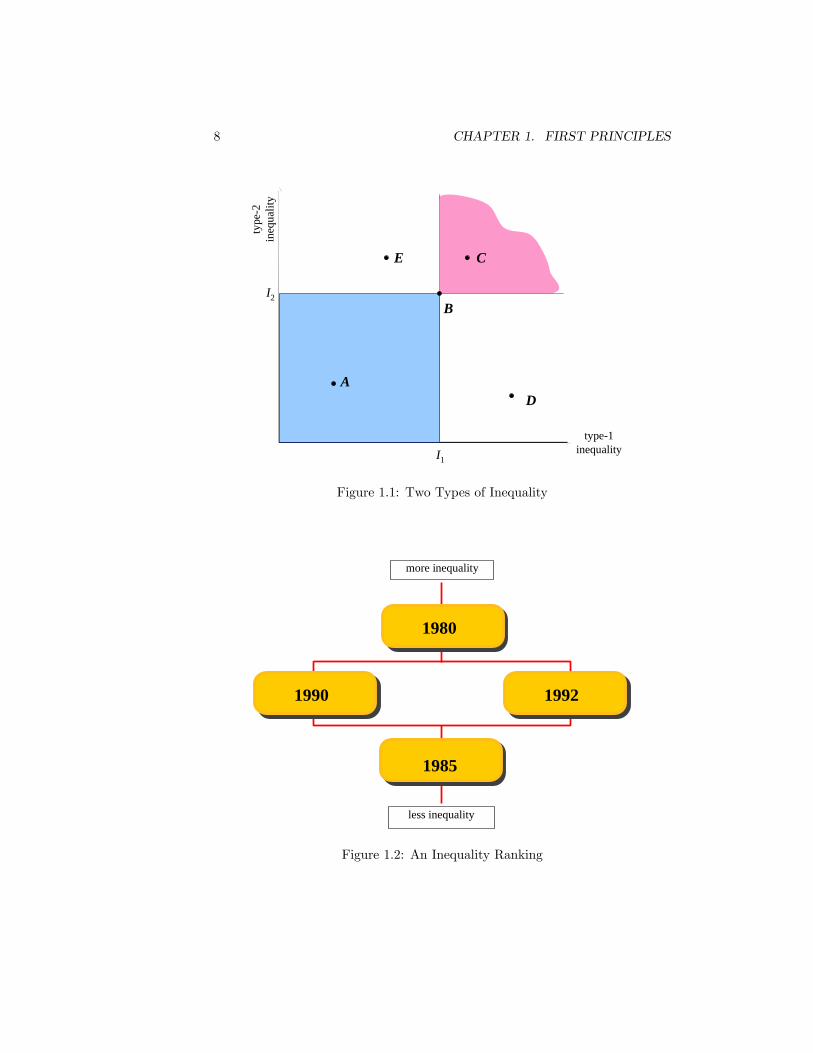
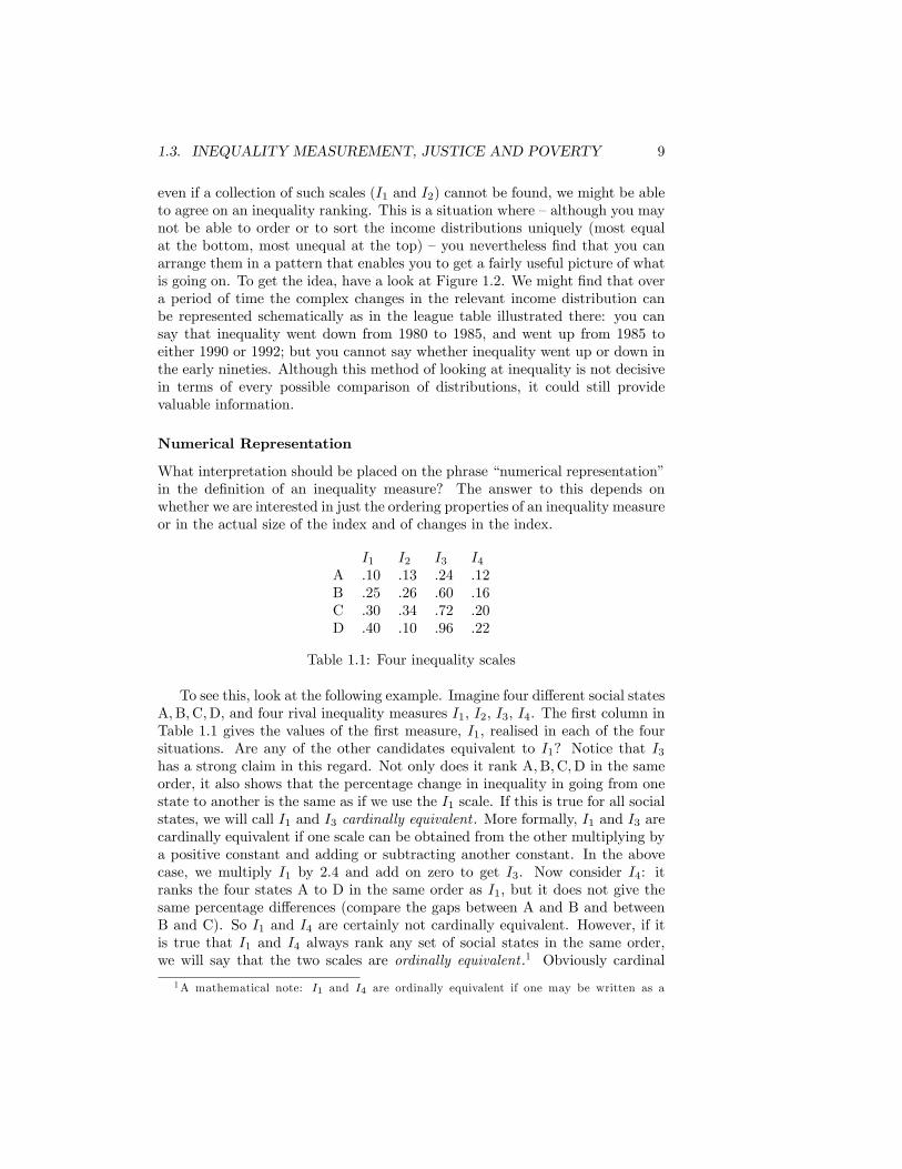
ity increased or decreased?�with a straight �yes�or �no.�But if we make theconcept of inequality multi-dimensional we greatly increase the possibility ofcoming up with ambiguous answers. For example, suppose we represent in-equality by two numbers, each describing a di¤erent aspect of inequality of thesame �income�attribute. We may depict this as a point such as B in Figure 1.1,which reveals that there is an amount I1 of type-1 inequality, and I2 of type-2inequality. Obviously all points like C represent states of society that are moreunequal than B and points such as A represent less unequal states. But it ismuch harder to compare B and D or to compare B and E. If we attempt toresolve this di¢ culty, we will �nd that we are e¤ectively using a single-numberrepresentation of inequality after all.Third, multi-number representations of income distributions may well have
their place alongside a standard scalar inequality measure. As we shall see inlater chapters, even if a single agreed number scale (I1 or I2) is unavailable, or
8 CHAPTER 1. FIRST PRINCIPLES
type
2in
equa
lity
I1
A
C
D
E
I2
type1inequality
B
Figure 1.1: Two Types of Inequality
1980
1985
1990 1992
more inequality
less inequality
Figure 1.2: An Inequality Ranking
1.3. INEQUALITY MEASUREMENT, JUSTICE AND POVERTY 9
even if a collection of such scales (I1 and I2) cannot be found, we might be ableto agree on an inequality ranking. This is a situation where �although you maynot be able to order or to sort the income distributions uniquely (most equalat the bottom, most unequal at the top) �you nevertheless �nd that you canarrange them in a pattern that enables you to get a fairly useful picture of whatis going on. To get the idea, have a look at Figure 1.2. We might �nd that overa period of time the complex changes in the relevant income distribution canbe represented schematically as in the league table illustrated there: you cansay that inequality went down from 1980 to 1985, and went up from 1985 toeither 1990 or 1992; but you cannot say whether inequality went up or down inthe early nineties. Although this method of looking at inequality is not decisivein terms of every possible comparison of distributions, it could still providevaluable information.
Numerical Representation
What interpretation should be placed on the phrase �numerical representation�in the de�nition of an inequality measure? The answer to this depends onwhether we are interested in just the ordering properties of an inequality measureor in the actual size of the index and of changes in the index.
I1 I2 I3 I4A :10 :13 :24 :12B :25 :26 :60 :16C :30 :34 :72 :20D :40 :10 :96 :22
Table 1.1: Four inequality scales
To see this, look at the following example. Imagine four di¤erent social statesA;B;C;D, and four rival inequality measures I1, I2, I3, I4. The �rst column inTable 1.1 gives the values of the �rst measure, I1, realised in each of the foursituations. Are any of the other candidates equivalent to I1? Notice that I3has a strong claim in this regard. Not only does it rank A;B;C;D in the sameorder, it also shows that the percentage change in inequality in going from onestate to another is the same as if we use the I1 scale. If this is true for all socialstates, we will call I1 and I3 cardinally equivalent . More formally, I1 and I3 arecardinally equivalent if one scale can be obtained from the other multiplying bya positive constant and adding or subtracting another constant. In the abovecase, we multiply I1 by 2:4 and add on zero to get I3. Now consider I4: itranks the four states A to D in the same order as I1, but it does not give thesame percentage di¤erences (compare the gaps between A and B and betweenB and C). So I1 and I4 are certainly not cardinally equivalent. However, if itis true that I1 and I4 always rank any set of social states in the same order,we will say that the two scales are ordinally equivalent .1 Obviously cardinal
1A mathematical note: I1 and I4 are ordinally equivalent if one may be written as a
10 CHAPTER 1. FIRST PRINCIPLES
equivalence entails ordinal equivalence, but not vice versa. Finally we note thatI2 is not ordinally equivalent to the others, although for all we know it may bea perfectly sensible inequality measure.Now let A be the year 1970, let B be 1960, and D be 1950. Given the
question, �Was inequality less in 1970 than it was in 1960?�, I1 produces thesame answer as any other ordinally equivalent measure (such as I3 or I4): �nu-merical representation�simply means a ranking. But, given the question, �Didinequality fall more in the 1960s than it did in the 1950s?�, I1 only yields thesame answer as other cardinally equivalent measures (I3 alone): here inequalityneeds to have the same kind of �numerical representation�as temperature on athermometer.
Income Di¤erences
Should any and every �income di¤erence�be re�ected in a measure of inequal-ity? The commonsense answer is �No�, for two basic reasons �need and merit.The �rst reason is the more obvious: large families and the sick need moreresources than the single, healthy person to support a particular economic stan-dard. Hence in a �just� allocation, we would expect those with such greaterneeds to have a higher income than other people; such income di¤erences wouldthus be based on a principle of justice, and should not be treated as inequali-ties. To cope with this di¢ culty one may adjust the income concept such thatallowance is made for diversity of need, as mentioned in the last section; this issomething which needs to be done with some care �as we will �nd in Chapter5 (see the discussion on page 106).The case for ignoring di¤erences on account of merit depends on the interpre-
tation attached to �equality.�One obviously rough-and-ready description of ajust allocation requires equal incomes for all irrespective of personal di¤erencesother than need. However, one may argue strongly that in a just allocationhigher incomes should be received by doctors, heroes, inventors, Stakhanovitesand other deserving persons. Unfortunately, in practice it is more di¢ cult tomake adjustments similar to those suggested in the case of need and, more gen-erally, even distinguishing between income di¤erences that do represent genuineinequalities and those that do not poses a serious problem.
Given Population
The last point about the de�nition of an inequality measure concerns the phrase�given population�and needs to be clari�ed in two ways. Firstly, when examin-ing the population over say a number of years, what shall we do about the e¤ecton measured inequality of persons who either enter or leave the population, orwhose status changes in some other relevant way? The usual assumption is that
monotonically increasing function of the other, say I1 = f(I4), where dI1=dI4 > 0. Anexample of such a function is log(I). I1 and I3 are cardinally equivalent if f takes thefollowing special form: I1 = a+ bI3, where b is a positive number.
1.3. INEQUALITY MEASUREMENT, JUSTICE AND POVERTY 11
as long as the overall structure of income di¤erences stays the same (regard-less of whether di¤erent personnel are now receiving those incomes), measuredinequality remains unaltered. Hence the phenomenon of social mobility withinor in and out of the population eludes the conventional method of measuringinequality, although some might argue that it is connected with inequality ofopportunity.2 Secondly, one is not exclusively concerned with inequality in thepopulation as a whole. It is useful to be able to decompose this �laterally�intoinequality within constituent groups, di¤erentiated regionally or demographi-cally, perhaps, and inequality between these constituent groups. Indeed, onceone acknowledges basic heterogeneities within the population, such as age or sex,awkward problems of aggregation may arise, although we shall ignore them. Itmay also be useful to decompose inequality �vertically� so that one looks atinequality within a subgroup of the rich, or of the poor, for example. Hence thespeci�cation of the given population is by no means a trivial prerequisite to theapplication of inequality measurement.
Although the de�nition has made it clear that an inequality measure callsfor a numerical scale, I have not suggested how this scale should be calibrated.Speci�c proposals for this will occupy Chapters 2 and 3, but a couple of basicpoints may be made here.You may have noticed just now that the notion of justice was slipped in while
income di¤erences were being considered. In most applications of inequalityanalysis social justice really ought to be centre stage. That more just societiesshould register lower numbers on the inequality scale evidently accords with anintuitive appreciation of the term �inequality.�But, on what basis should prin-ciples of distributional justice and concern for inequality be based? Economicphilosophers have o¤ered a variety of answers. This concern could be no morethan the concern about the everyday risks of life: just as individuals are upsetby the �nancial consequences having their car stolen or missing their plane sotoo they would care about the hypothetical risk of drawing a losing ticket ina lottery of life chances; this lottery could be represented by the income dis-tribution in the UK, the USA or wherever; nice utilitarian calculations on thebalance of small-scale gains and losses become utilitarian calculations about lifechances; aversion to risk translates into aversion to inequality. Or the concerncould be based upon the altruistic feelings of each human towards his fellowsthat motivates charitable action. Or again it could be that there is a social im-perative toward concern for the least advantaged �and perhaps concern aboutthe inordinately rich � that transcends the personal twinges of altruism andenvy. It could be simple concern about the possibility of social unrest. It ispossible to construct a coherent justice-based theory of inequality measurementon each of these notions, although that takes us beyond the remit of this book.However, if we can clearly specify what a just distribution is, such a state
provides the zero from which we start our inequality measure. But even awell-de�ned principle of distributive justice is not su¢ cient to enable one to
2Check question 6 at the end of the chapter to see if you concur with this view.
12 CHAPTER 1. FIRST PRINCIPLES
mark o¤ an inequality scale unambiguously when considering diverse unequalsocial states. Each of the apparently contradictory scales I1 and I2 consideredin Figure 1.1 and Table 1.1 might be solidly founded on the same principle ofjustice, unless such a principle were extremely narrowly de�ned.The other general point is that we might suppose there is a close link be-
tween an indicator of the extent of poverty and the calibration of a measureof economic inequality. This is not necessarily so, because two rather di¤erentproblems are generally involved. In the case of the measurement of poverty,one is concerned primarily with that segment of the population falling belowsome speci�ed �poverty line�; to obtain the poverty measure one may performa simple head count of this segment, or calculate the gap between the averageincome of the poor and the average income of the general population, or carryout some other computation on poor people�s incomes in relation to each otherand to the rest of the population. Now in the case of inequality one generallywishes to capture the e¤ects of income di¤erences over a much wider range.Hence it is perfectly possible for the measured extent of poverty to be decliningover time, while at the same time and in the same society measured inequalityincreases due to changes in income di¤erences within the non-poor segment ofthe population, or because of migrations between the two groups. (If you arein doubt about this you might like to have a look at question 5 on page 13.)Poverty will make a few guest appearances in the course of this book, but onthe whole our discussion of inequality has to take a slightly di¤erent track fromthe measurement of poverty.
1.4 Inequality and the social structure
Finally we return to the subject of the �rst ingredient, namely the basic socialunits used in studying inequality �or the elementary particles of which we imag-ine society to be constituted. The de�nition of the social unit, whether it be asingle person, a nuclear family or an extended family depends intrinsically uponthe social context, and upon the interpretation of inequality that we impose.Although it may seem natural to adopt an individualistic approach, some other�collective�unit may be more appropriate.When economic inequality is our particular concern, the theory of the devel-
opment of the distribution of income or wealth may itself in�uence the choiceof the basic social unit. To illustrate this, consider the classical view of an eco-nomic system, the population being subdivided into distinct classes of workers,capitalists and landowners. Each class is characterised by a particular functionin the economic order and by an associated type of income �wages, pro�ts,and rents. If, further, each is regarded as internally fairly homogeneous, thenit makes sense to pursue the analysis of inequality in class terms rather than interms of individual units.However, so simple a model is unsuited to describing inequality in a signif-
icantly heterogeneous society, despite the potential usefulness of class analysisfor other social problems. A super�cial survey of the world around us reveals

1.5. QUESTIONS 13
rich and poor workers, failed and successful capitalists and several people whoserôles and incomes do not �t into neat slots. Hence the focus of attention in thisbook is principally upon individuals rather than types whether the analysis isinterpreted in terms of economic inequality or some other sense.Thus reduced to its essentials it might appear that we are dealing with a
purely formal problem, which sounds rather dull. This is not so. Although thesubject matter of this book is largely technique, the techniques involved areessential for coping with the analysis of many social and economic problems ina systematic fashion; and these problems are far from dull or uninteresting.
1.5 Questions
1. In Syldavia the economists �nd that (annual) household consumption c isrelated to (annual) income y by the formula
c = �+ �y;
where � > 0 and 0 < � < 1. Because of this, they argue, inequality ofconsumption must be less than inequality of income. Provide an intuitiveargument for this.
2. Ruritanian society consists of three groups of people: Artists, Bureaucratsand Chocolatiers. Each Artist has high income (15 000 Ruritanian Marks)with a 50% probability, and low income (5 000 RM) with 50% probability.Each Bureaucrat starts working life on a salary of 5 000 RM and thenbene�ts from an annual increment of 250 RM over the 40 years of his(perfectly safe) career. Chocolatiers get a straight annual wage of 10 000RM. Discuss the extent of inequality in Ruritania according to annualincome and lifetime income concepts.
3. In Borduria the government statistical service uses an inequality indexthat in principle can take any value greater than or equal to 0. You wantto introduce a transformed inequality index that is ordinally equivalentto the original but that will always lie between zero and 1. Which of thefollowing will do?
1
I + 1;
r1
I + 1;
I
I � 1 ;pI:
4. Methods for analysing inequality of income could be applied to inequalityof use of speci�c health services (Williams and Doessel 2006). What wouldbe the principal problems of trying to apply these methods to inequalityof health status?
5. After a detailed study of a small village, Government experts reckon thatthe poverty line is 100 rupees a month. In January a joint team from theMinistry of Food and the Central Statistical O¢ ce carry out a survey ofliving standards in the village: the income for each villager (in rupees per
14 CHAPTER 1. FIRST PRINCIPLES
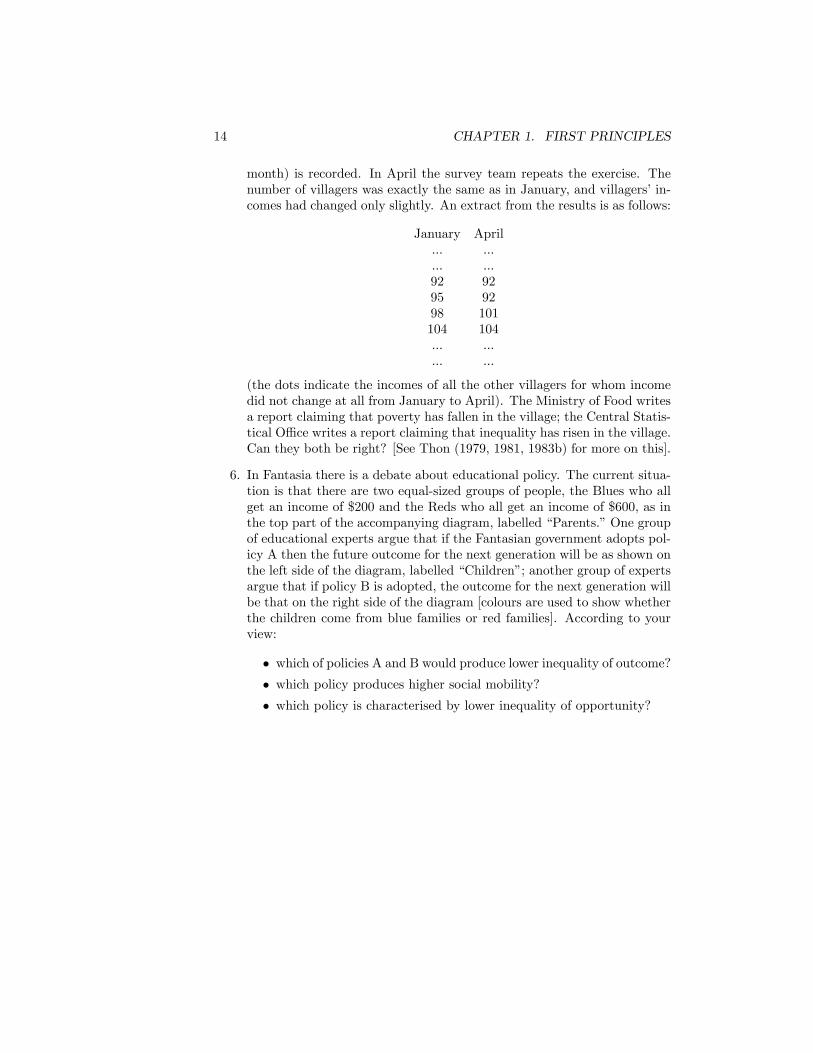
month) is recorded. In April the survey team repeats the exercise. Thenumber of villagers was exactly the same as in January, and villagers�in-comes had changed only slightly. An extract from the results is as follows:
January April::: :::::: :::92 9295 9298 101104 104::: :::::: :::
(the dots indicate the incomes of all the other villagers for whom incomedid not change at all from January to April). The Ministry of Food writesa report claiming that poverty has fallen in the village; the Central Statis-tical O¢ ce writes a report claiming that inequality has risen in the village.Can they both be right? [See Thon (1979, 1981, 1983b) for more on this].
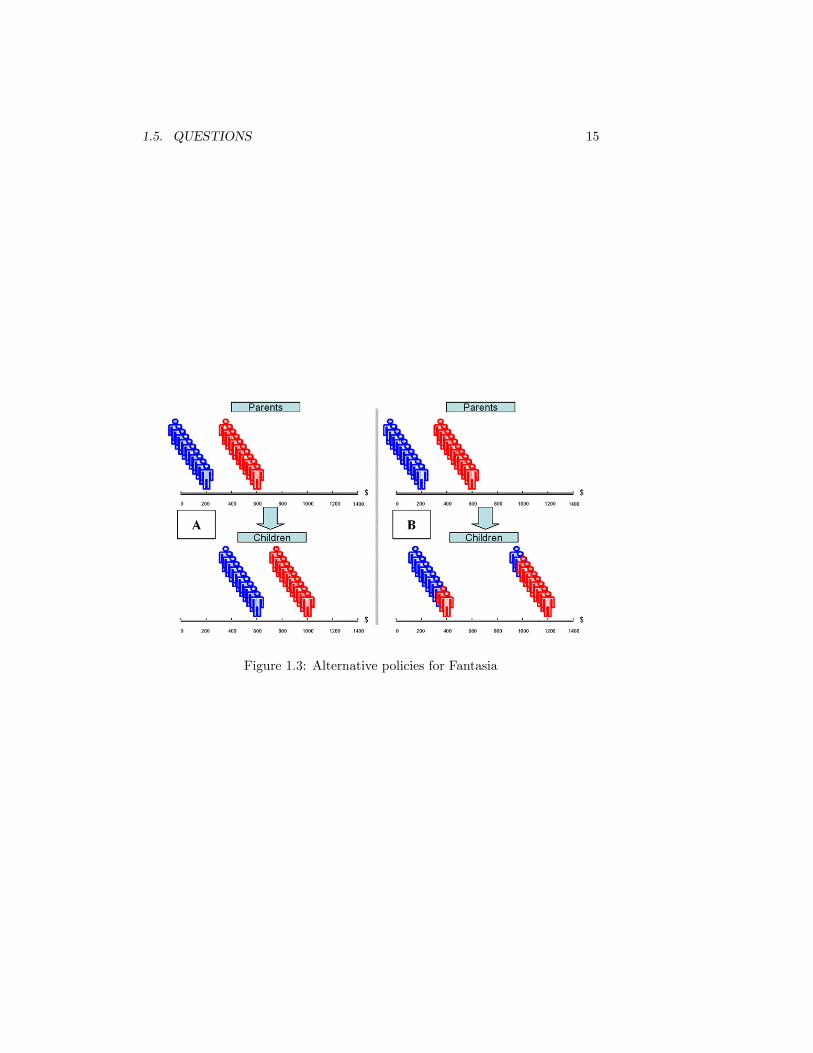
6. In Fantasia there is a debate about educational policy. The current situa-tion is that there are two equal-sized groups of people, the Blues who allget an income of $200 and the Reds who all get an income of $600, as inthe top part of the accompanying diagram, labelled �Parents.�One groupof educational experts argue that if the Fantasian government adopts pol-icy A then the future outcome for the next generation will be as shown onthe left side of the diagram, labelled �Children�; another group of expertsargue that if policy B is adopted, the outcome for the next generation willbe that on the right side of the diagram [colours are used to show whetherthe children come from blue families or red families]. According to yourview:
� which of policies A and B would produce lower inequality of outcome?� which policy produces higher social mobility?� which policy is characterised by lower inequality of opportunity?
1.5. QUESTIONS 15
Figure 1.3: Alternative policies for Fantasia

16 CHAPTER 1. FIRST PRINCIPLES
Chapter 2
Charting Inequality
F. Scott Fitzgerald: �The rich are di¤erent from us.�Ernest Hemingway: �Yes, they have more money.�
If society really did consist of two or three fairly homogeneous groups, econo-mists and others could be saved a lot of trouble. We could then simply look atthe division of income between landlords and peasants, among workers, capi-talists and rentiers, or any other appropriate sections. Naturally we would stillbe faced with such fundamental issues as how much each group should possessor receive, whether the statistics are reliable and so on, but questions such as�what is the income distribution?� could be satisfactorily met with a snappyanswer �65% to wages, 35% to pro�ts.�Of course matters are not that simple.As we have argued, we want a way of looking at inequality that re�ects boththe depth of poverty of the �have nots�of society and the height of well-beingof the �haves�: it is not easy to do this just by looking at the income accruingto, or the wealth possessed by, two or three groups.So in this chapter we will look at several quite well-known ways of presenting
inequality in a large heterogeneous group of people. They are all methods ofappraising the sometimes quite complicated information that is contained inan income distribution, and they can be grouped under three broad headings:diagrams, inequality measures, and rankings. To make the exposition easier Ishall continue to refer to �income distribution�, but you should bear in mind, ofcourse, that the principles can be carried over to the distribution of any othervariable that you can measure and that you think is of economic interest.
2.1 Diagrams
Putting information about income distribution into diagrammatic form is a par-ticularly instructive way of representing some of the basic ideas about inequality.There are several useful ways of representing inequality in pictures; the four that
17
18 CHAPTER 2. CHARTING INEQUALITY
I shall discuss are introduced in the accompanying box. Let us have a closerlook at each of them.
� Parade of Dwarfs� Frequency distribution� Lorenz Curve� Log transformation
PICTURES OF INEQUALITY
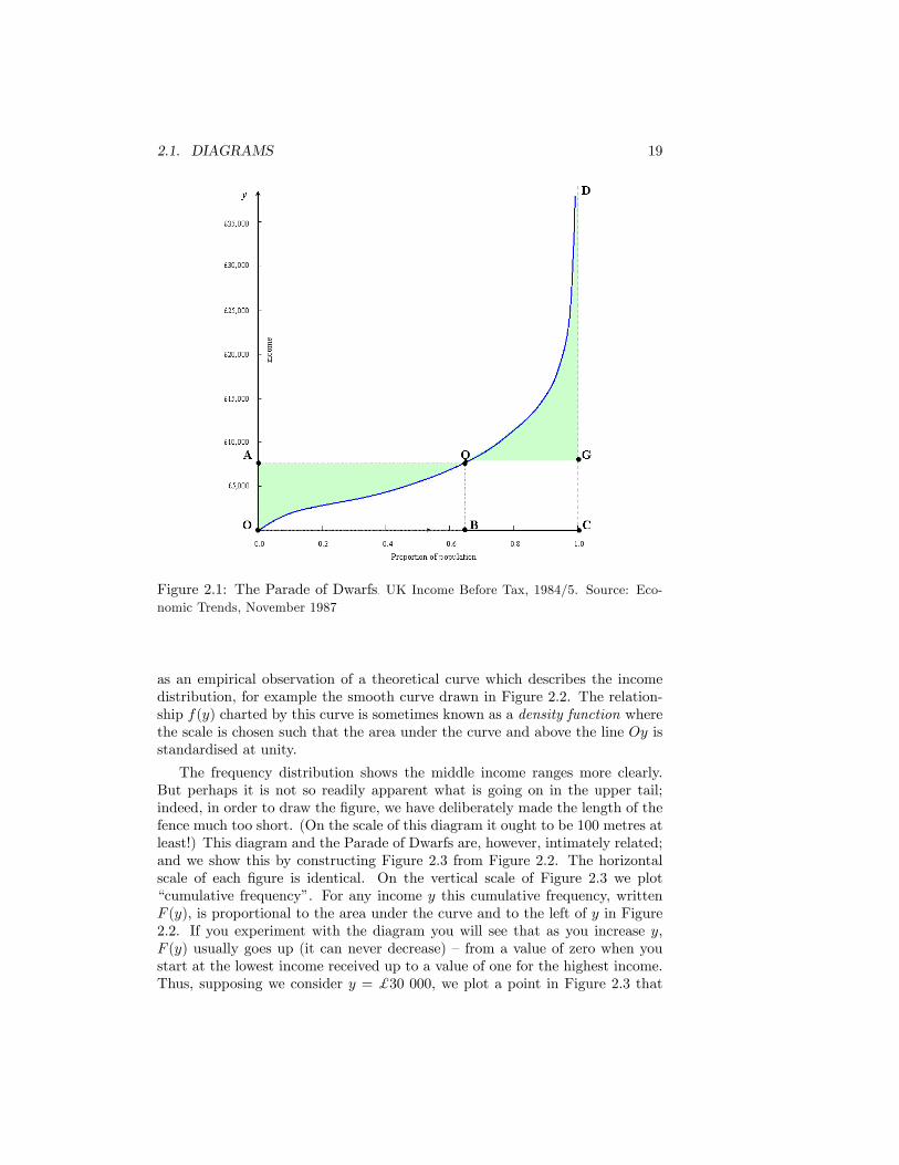
Jan Pen�s Parade of Dwarfs is one of the most persuasive and attractivevisual aids in the subject of income distribution. Suppose that everyone in thepopulation had a height proportional to his or her income, with the person onaverage income being endowed with average height. Line people up in order ofheight and let them march past in some given time interval � let us say onehour. Then the sight that would meet our eyes is represented by the curve inFigure 2.1.1 The whole parade passes in the interval represented by OC. But wedo not meet the person with average income until we get to the point B (whenwell over half the parade has gone by). Divide total income by total population:this gives average or mean income (�y) and is represented by the height OA.We have oversimpli�ed Pen�s original diagram by excluding from considerationpeople with negative reported incomes, which would involve the curve crossingthe base line towards its left-hand end. And in order to keep the diagram on thepage, we have plotted the last point of the curve (D) in a position that wouldbe far too low in practice.This diagram highlights the presence of any extremely large incomes and to
a certain extent abnormally small incomes. But we may have reservations aboutthe degree of detail that it seems to impart concerning middle income receivers.We shall see this point recur when we use this diagram to derive an inequalitymeasure that informs us about changes in the distribution.Frequency distributions are well-tried tools of statisticians, and are discussed
here mainly for the sake of completeness and as an introduction for those un-familiar with the concept � for a fuller account see the references cited in thenotes to this chapter. An example is found in Figure 2.2. Suppose you werelooking down on a �eld. On one side, the axis Oy, there is a long straight fencemarked o¤ income categories: the physical distance between any two pointsalong the fence directly corresponds to the income di¤erences they represent.Then get the whole population to come into the �eld and line up in the strip ofland marked o¤ by the piece of fence corresponding to their income bracket. Sothe £ 10,000-to-£ 12,500-a-year persons stand on the shaded patch. The shapethat you get will resemble the stepped line in Figure 2.2 �called a histogram�which represents the frequency distribution. It may be that we regard this
1Those with especially sharp eyes will see that the source is more than 20 years old. Thereis a good reason for using these data �see the notes on page 179.
2.1. DIAGRAMS 19
Figure 2.1: The Parade of Dwarfs. UK Income Before Tax, 1984/5. Source: Eco-nomic Trends, November 1987
as an empirical observation of a theoretical curve which describes the incomedistribution, for example the smooth curve drawn in Figure 2.2. The relation-ship f(y) charted by this curve is sometimes known as a density function wherethe scale is chosen such that the area under the curve and above the line Oy isstandardised at unity.
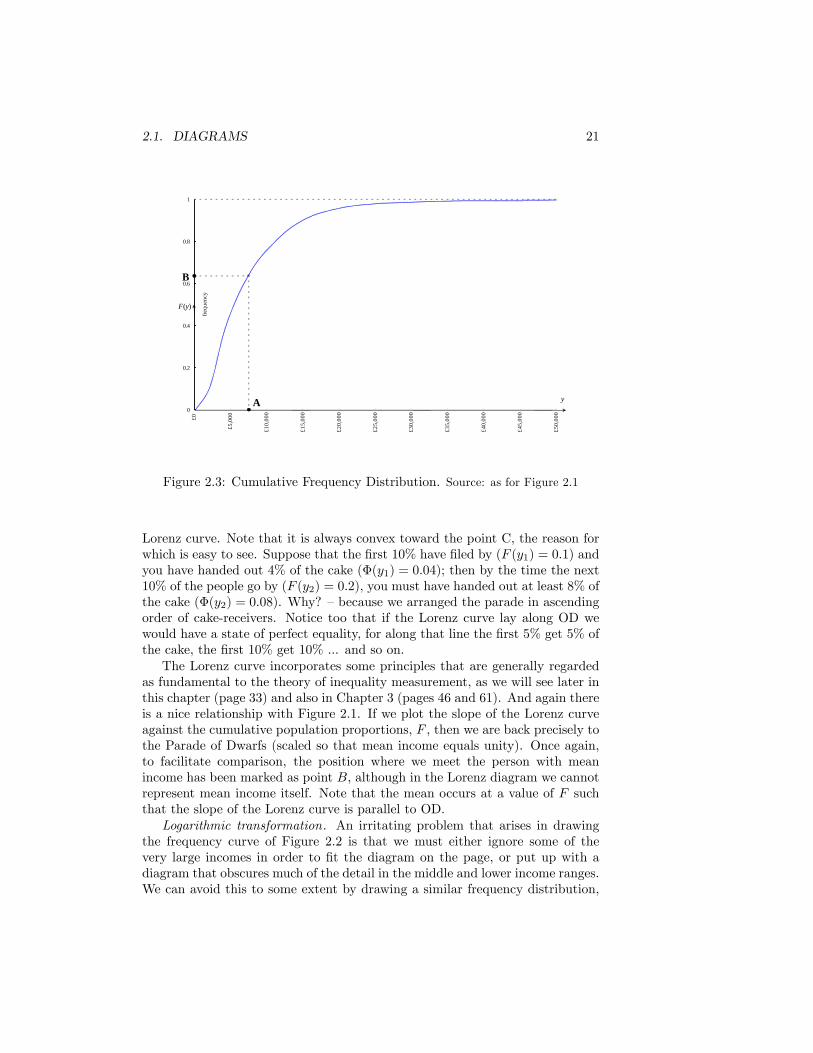
The frequency distribution shows the middle income ranges more clearly.But perhaps it is not so readily apparent what is going on in the upper tail;indeed, in order to draw the �gure, we have deliberately made the length of thefence much too short. (On the scale of this diagram it ought to be 100 metres atleast!) This diagram and the Parade of Dwarfs are, however, intimately related;and we show this by constructing Figure 2.3 from Figure 2.2. The horizontalscale of each �gure is identical. On the vertical scale of Figure 2.3 we plot�cumulative frequency�. For any income y this cumulative frequency, writtenF (y), is proportional to the area under the curve and to the left of y in Figure2.2. If you experiment with the diagram you will see that as you increase y,F (y) usually goes up (it can never decrease) � from a value of zero when youstart at the lowest income received up to a value of one for the highest income.Thus, supposing we consider y = $30 000, we plot a point in Figure 2.3 that

20 CHAPTER 2. CHARTING INEQUALITY
Figure 2.2: Frequency Distribution of Income Source: as for Figure 2.1
corresponds to the proportion of the population with $30 000 or less. And wecan repeat this operation for every point on either the empirical curve or on thesmooth theoretical curve.
The visual relationship between Figures 2.1 and 2.3 is now obvious. As afurther point of reference, the position of mean income has been drawn in atthe point A in the two �gures. (If you still don�t see it, try turning the pageround!).
The Lorenz curve was introduced in 1905 as a powerful method of illustratingthe inequality of the wealth distribution. A simpli�ed explanation of it runs asfollows.
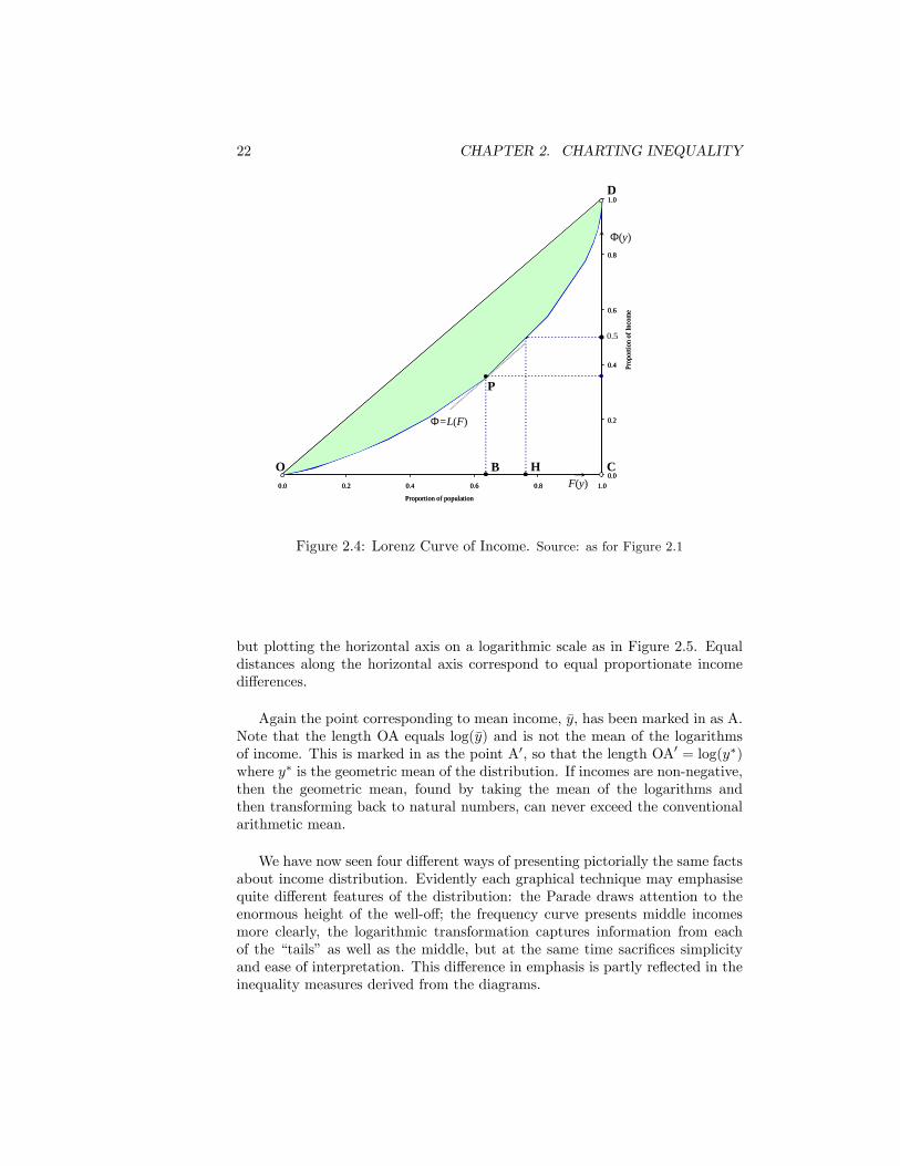
Once again line up everybody in ascending order of incomes and let themparade by. Measure F (y), the proportion of people who have passed by, alongthe horizontal axis of Figure 2.4. Once point C is reached everyone has goneby, so F (y) = 1. Now as each person passes, hand him his share of the �cake��i.e. the proportion of total income that he receives. When the parade reachespeople with income y, let us suppose that a proportion �(y) of the cake hasgone. So of course when F (y) = 0, �(y) is also 0 (no cake gone); and whenF (y) = 1, �(y) is also 1 (all the cake has been handed out). �(y) is measuredon the vertical scale in Figure 2.4, and the graph of � plotted against F is the
2.1. DIAGRAMS 21
0
0.2
0.4
0.6
0.8
1£0
£5,0
00
£10,
000
£15,
000
£20,
000
£25,
000
£30,
000
£35,
000
£40,
000
£45,
000
£50,
000
frequ
ency
F(y)
yA
B
Figure 2.3: Cumulative Frequency Distribution. Source: as for Figure 2.1
Lorenz curve. Note that it is always convex toward the point C, the reason forwhich is easy to see. Suppose that the �rst 10% have �led by (F (y1) = 0:1) andyou have handed out 4% of the cake (�(y1) = 0:04); then by the time the next10% of the people go by (F (y2) = 0:2), you must have handed out at least 8% ofthe cake (�(y2) = 0:08). Why? �because we arranged the parade in ascendingorder of cake-receivers. Notice too that if the Lorenz curve lay along OD wewould have a state of perfect equality, for along that line the �rst 5% get 5% ofthe cake, the �rst 10% get 10% ... and so on.The Lorenz curve incorporates some principles that are generally regarded
as fundamental to the theory of inequality measurement, as we will see later inthis chapter (page 33) and also in Chapter 3 (pages 46 and 61). And again thereis a nice relationship with Figure 2.1. If we plot the slope of the Lorenz curveagainst the cumulative population proportions, F , then we are back precisely tothe Parade of Dwarfs (scaled so that mean income equals unity). Once again,to facilitate comparison, the position where we meet the person with meanincome has been marked as point B, although in the Lorenz diagram we cannotrepresent mean income itself. Note that the mean occurs at a value of F suchthat the slope of the Lorenz curve is parallel to OD.Logarithmic transformation. An irritating problem that arises in drawing
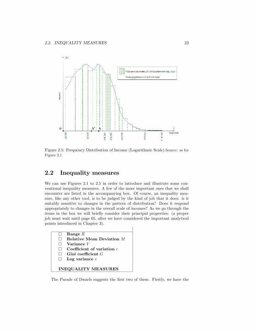
the frequency curve of Figure 2.2 is that we must either ignore some of thevery large incomes in order to �t the diagram on the page, or put up with adiagram that obscures much of the detail in the middle and lower income ranges.We can avoid this to some extent by drawing a similar frequency distribution,
22 CHAPTER 2. CHARTING INEQUALITY
0.0
0.2
0.4
0.6
0.8
1.0
0.0 0.2 0.4 0.6 0.8 1.0
Proportion of population
Prop
ortio
n of
Inco
me
0.0
0.2
0.4
0.6
0.8
1.0
0.0 0.2 0.4 0.6 0.8 1.0
Proportion of population
Prop
ortio
n of
Inco
me
Φ=L(F)
Φ(y)
F(y)O B
D
P
H
0.5
C
Figure 2.4: Lorenz Curve of Income. Source: as for Figure 2.1
but plotting the horizontal axis on a logarithmic scale as in Figure 2.5. Equaldistances along the horizontal axis correspond to equal proportionate incomedi¤erences.
Again the point corresponding to mean income, �y, has been marked in as A.Note that the length OA equals log(�y) and is not the mean of the logarithmsof income. This is marked in as the point A0, so that the length OA0 = log(y�)where y� is the geometric mean of the distribution. If incomes are non-negative,then the geometric mean, found by taking the mean of the logarithms andthen transforming back to natural numbers, can never exceed the conventionalarithmetic mean.
We have now seen four di¤erent ways of presenting pictorially the same factsabout income distribution. Evidently each graphical technique may emphasisequite di¤erent features of the distribution: the Parade draws attention to theenormous height of the well-o¤; the frequency curve presents middle incomesmore clearly, the logarithmic transformation captures information from eachof the �tails� as well as the middle, but at the same time sacri�ces simplicityand ease of interpretation. This di¤erence in emphasis is partly re�ected in theinequality measures derived from the diagrams.
2.2. INEQUALITY MEASURES 23
Figure 2.5: Frequency Distribution of Income (Logarithmic Scale).Source: as forFigure 2.1
2.2 Inequality measures
We can use Figures 2.1 to 2.5 in order to introduce and illustrate some con-ventional inequality measures. A few of the more important ones that we shallencounter are listed in the accompanying box. Of course, an inequality mea-sure, like any other tool, is to be judged by the kind of job that it does: is itsuitably sensitive to changes in the pattern of distribution? Does it respondappropriately to changes in the overall scale of incomes? As we go through theitems in the box we will brie�y consider their principal properties: (a properjob must wait until page 65, after we have considered the important analyticalpoints introduced in Chapter 3).
� Range R� Relative Mean Deviation M� Variance V� Coe¢ cient of variation c� Gini coe¢ cient G� Log variance v
INEQUALITY MEASURES
The Parade of Dwarfs suggests the �rst two of these. Firstly, we have the
24 CHAPTER 2. CHARTING INEQUALITY
range, which we de�ne simply as the distance CD in Figure 2.1 or:
R = ymax � ymin;
where ymax and ymin are, respectively the maximum and minimum values ofincome in the parade (we may, of course standardise by considering R=ymin orR=�y). Plato apparently had this concept in mind when he made the followingjudgement:
We maintain that if a state is to avoid the greatest plague of all �I mean civil war, though civil disintegration would be a better term�extreme poverty and wealth must not be allowed to arise in anysection of the citizen-body, because both lead to both these disasters.That is why the legislator must now announce the acceptable limitsof wealth and poverty. The lower limit of poverty must be the valueof the holding. The legislator will use the holding as his unit ofmeasure and allow a man to possess twice, thrice, and up to fourtimes its value. �The Laws, 745.
The problems with the range are evident. Although it might be satisfactoryin a small closed society where everyone�s income is known fairly certainly, itis clearly unsuited to large, heterogeneous societies where the �minimum�and�maximum�incomes can at best only be guessed. The measure will be highlysensitive to the guesses or estimates of these two extreme values. In practice onemight try to get around the problem by using a related concept that is morerobust: take the gap between the income of the person who appears exactlyat, say, the end of the �rst three minutes in the Parade, and that of the personexactly at the 57th minute (the bottom 5% and the top 5% of the line of people)or the income gap between the people at the 6th and 54th minute (the bottom10% and the top 10% of the line of people). However, even if we did that there isa more compelling reason for having doubts about the usefulness of R. Supposewe can wave a wand and bring about a society where the person at position Oand the person at position C are left at the same height, but where everyone elsein between was levelled to some equal, intermediate height. We would probablyagree that inequality had been reduced, though not eliminated. But accordingto R it is just the same!You might be wondering whether the problem with R arises because it
ignores much of the information about the distribution (it focuses just on acouple of extreme incomes). Unfortunately we shall �nd a similar criticism insubtle form attached to the second inequality measure that we can read o¤ theParade diagram, one that uses explicitly the income values of all the individu-als. This is the relative mean deviation, which is de�ned as the average absolutedistance of everyone�s income from the mean, expressed as a proportion of themean. Take a look at the shaded portions in Figure 2.1. These portions, whichare necessarily of equal size, constitute the area between the Parade curve itselfand the horizontal line representing mean income. In some sense, the larger isthis area, the greater is inequality. (Try drawing the Parade with more giants
2.2. INEQUALITY MEASURES 25
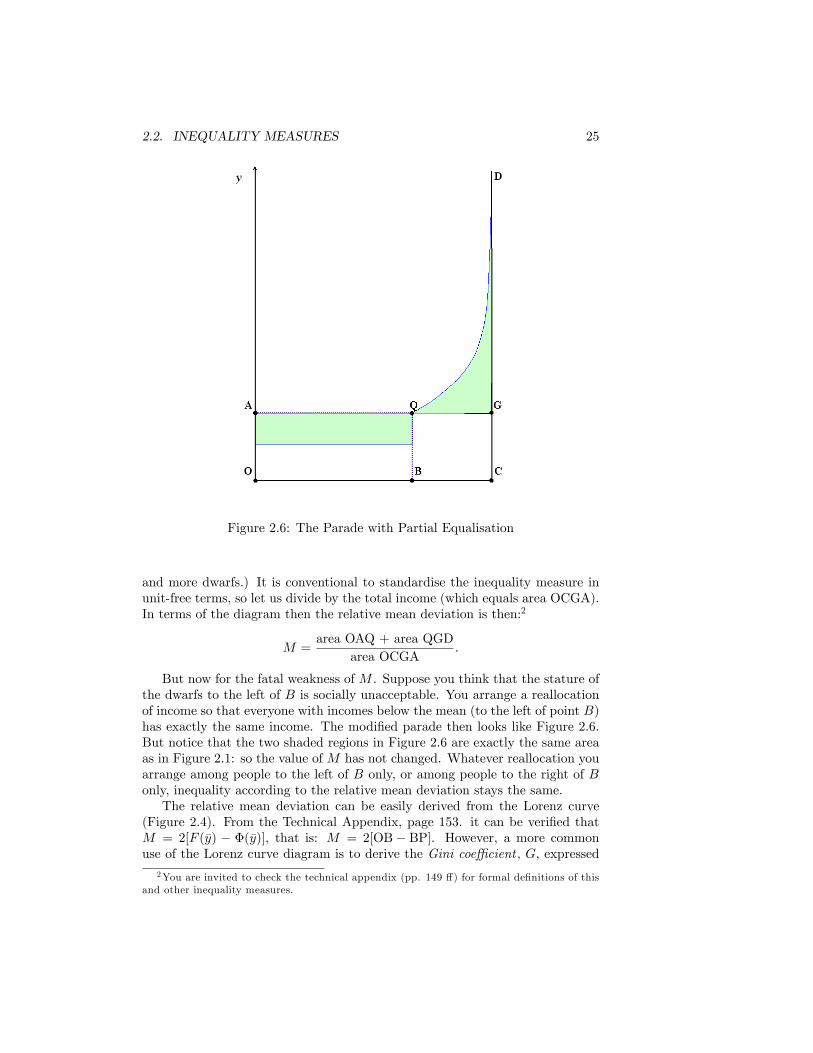
Figure 2.6: The Parade with Partial Equalisation
and more dwarfs.) It is conventional to standardise the inequality measure inunit-free terms, so let us divide by the total income (which equals area OCGA).In terms of the diagram then the relative mean deviation is then:2
M =area OAQ + area QGD
area OCGA:
But now for the fatal weakness of M . Suppose you think that the stature ofthe dwarfs to the left of B is socially unacceptable. You arrange a reallocationof income so that everyone with incomes below the mean (to the left of point B)has exactly the same income. The modi�ed parade then looks like Figure 2.6.But notice that the two shaded regions in Figure 2.6 are exactly the same areaas in Figure 2.1: so the value of M has not changed. Whatever reallocation youarrange among people to the left of B only, or among people to the right of Bonly, inequality according to the relative mean deviation stays the same.The relative mean deviation can be easily derived from the Lorenz curve
(Figure 2.4). From the Technical Appendix, page 153. it can be veri�ed thatM = 2[F (�y) � �(�y)], that is: M = 2[OB� BP]. However, a more commonuse of the Lorenz curve diagram is to derive the Gini coe¢ cient , G, expressed
2You are invited to check the technical appendix (pp. 149 ¤) for formal de�nitions of thisand other inequality measures.
26 CHAPTER 2. CHARTING INEQUALITY
as the ratio of the shaded area in Figure 2.4 to the area OCD. There is avariety of equivalent ways of de�ning G; but perhaps the easiest de�nition is asthe average di¤erence between all possible pairs of incomes in the population,expressed as a proportion of total income: see pages 151 and 153 for a formalde�nition. The main disadvantage of G is that it places a rather curious implicitrelative value on changes that may occur in di¤erent parts of the distribution.An income transfer from a relatively rich person to a person with £ x less hasa much greater e¤ect on G if the two persons are near the middle rather thanat either end of the parade.3 So, consider transferring £ 1 from a person with£ 10 100 to a person with £ 10 000. This has a much greater e¤ect on reducingG than transferring £ 1 from a person with £ 1 100 to one with £ 1 000 or thantransferring £ 1 from a person with £ 100 100 to a person with £ 100 000. Thisvaluation may be desirable, but it is not obvious that it is desirable: this pointabout the valuation of transfers is discussed more fully in Chapter 3 once wehave discussed social welfare explicitly.Other inequality measures can be derived from the Lorenz curve in Figure
2.4. Two have been suggested in connection with the problem of measuringinequality in the distribution of power, as re�ected in voting strength. Firstly,consider the income level y0 at which half the national cake has been distrib-uted to the parade; i.e. �(y0) = 1
2 . Then de�ne the minimal majority inequalitymeasure as F (y0), which is the distance OH. If � is reinterpreted as the pro-portion of seats in an elected assembly where the votes are spread unevenlyamong the constituencies as re�ected by the Lorenz curve, and if F is reinter-preted as a proportion of the electorate, then 1� F (y0) represents the smallestproportion of the electorate that can secure a majority in the elected assembly.Secondly, we have the equal shares coe¢ cient, de�ned as F (�y): the proportionof the population that has income �y or less (the distance OB), or the proportionof the population that has �average voting strength� or less. Clearly, eitherof these measures as applied to the distribution of income or wealth is subjectto essentially the same criticism as the relative mean deviation: they are in-sensitive to transfers among members of the Parade on the same side of theperson with income y0 (in the case of the minimal majority measure) or �y (theequal shares coe¢ cient): in e¤ect they measure changes in inequality by onlyrecording transfers between two broadly based groups.Now let us consider Figures 2.2 and 2.5: the frequency distribution and its
log-transformation. An obvious suggestion is to measure inequality in the sameway as statisticians measure dispersion of any frequency distribution. In thisapplication, the usual method would involve measuring the distance between
3To see why, check the de�nition of G on page 151 and note the formula for the �TransferE¤ect� (right-hand column). Now imagine persons i and j located at two points yi and yj , agiven distance x apart, along the fence described on page 18; if there are lots of other personsin the part of the �eld between those two points then the transfer-e¤ect formula tells us thatthe impact of a transfer from i to j will be large (F (yj)� F (yi) is a large number) and viceversa. It so happens that real-world frequency distributions of income look like that in Figure2.2 (with a peak in the mid-income range rather than at either end), so that two incomereceivers, £ 100 apart, have many people between them if they are located in the mid-incomerange but rather few people between them if located at one end or other.
2.2. INEQUALITY MEASURES 27
the individual�s income yi and mean income �y, squaring this, and then �ndingthe average of the resulting quantity in the whole population. Assuming thatthere are n people we de�ne the variance:
V =1
n
nXi=1
[yi � �y]2: (2.1)
However, V is unsatisfactory in that were we simply to double everyone�sincomes (and thereby double mean income and leave the shape of the distribu-tion essentially unchanged), V would quadruple. One way round this problemis to standardise V . De�ne the coe¢ cient of variation thus
c =
pV
�y: (2.2)
Another way to avoid this problem is to look at the variance in terms ofthe logarithms of income � to apply the transformation illustrated in Figure2.5 before evaluating the inequality measure. In fact there are two importantde�nitions:
v =1
n
nXi=1
�log
�yi�y
��2; (2.3)
v1 =1
n
nXi=1
�log
�yiy�
��2: (2.4)
The �rst of these we will call the logarithmic variance, and the second we maymore properly term the variance of the logarithms of incomes. Note that v isde�ned relative to the logarithm of mean income; v1 is de�ned relative to themean of the logarithm of income. Either de�nition is invariant under propor-tional increases in all incomes.We shall �nd that v1 has much to recommend it when we come to examine
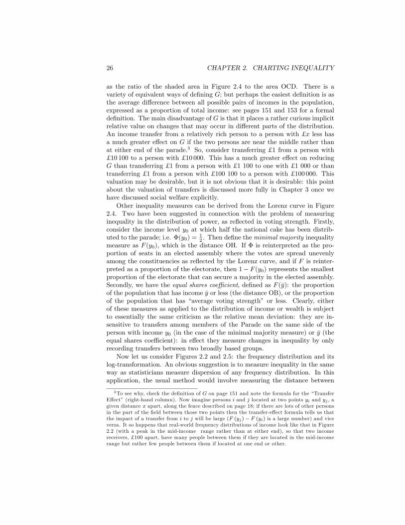
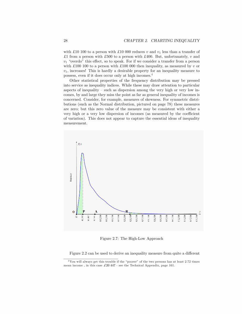
the lognormal distribution in Chapter 4. However, c; v and v1 can be criticisedmore generally on grounds similar to those on which G was criticised. Considera transfer of £ 1 from a person with y to a person with y�$100. How does thistransfer a¤ect these inequality measures? In the case of c, it does not matterin the slightest where in the parade this transfer is e¤ected: so whether thetransfer is from a person with £ 500 to a person with £ 400, or from a personwith £ 100 100 to a person with £ 100 000, the reduction in c is exactly thesame. Thus c will be particularly good at capturing inequality among highincomes, but may be of more limited use in re�ecting inequality elsewhere inthe distribution. In contrast to this property of c, there appears to be goodreason to suggest that a measure of inequality have the property that a transferof the above type carried out in the low income brackets would be quantitativelymore e¤ective in reducing inequality than if the transfer were carried out in thehigh income brackets. The measures v and v1 appear to go some way towardsmeeting this objection. Taking the example of the UK in 1984/5 (illustrated inFigures 2.1 to 2.5 where we have �y = £ 7 522), a transfer of £ 1 from a person
28 CHAPTER 2. CHARTING INEQUALITY
with £ 10 100 to a person with £ 10 000 reduces v and v1 less than a transfer of£ 1 from a person with £ 500 to a person with £ 400. But, unfortunately, v andv1 �overdo�this e¤ect, so to speak. For if we consider a transfer from a personwith £ 100 100 to a person with £ 100 000 then inequality, as measured by v orv1, increases! This is hardly a desirable property for an inequality measure topossess, even if it does occur only at high incomes.4
Other statistical properties of the frequency distribution may be pressedinto service as inequality indices. While these may draw attention to particularaspects of inequality �such as dispersion among the very high or very low in-comes, by and large they miss the point as far as general inequality of incomes isconcerned. Consider, for example, measures of skewness. For symmetric distri-butions (such as the Normal distribution, pictured on page 78) these measuresare zero; but this zero value of the measure may be consistent with either avery high or a very low dispersion of incomes (as measured by the coe¢ cientof variation). This does not appear to capture the essential ideas of inequalitymeasurement.
Figure 2.7: The High-Low Approach
Figure 2.2 can be used to derive an inequality measure from quite a di¤erent
4You will always get this trouble if the �poorer�of the two persons has at least 2.72 timesmean income , in this case $20 447 - see the Technical Appendix, page 161.
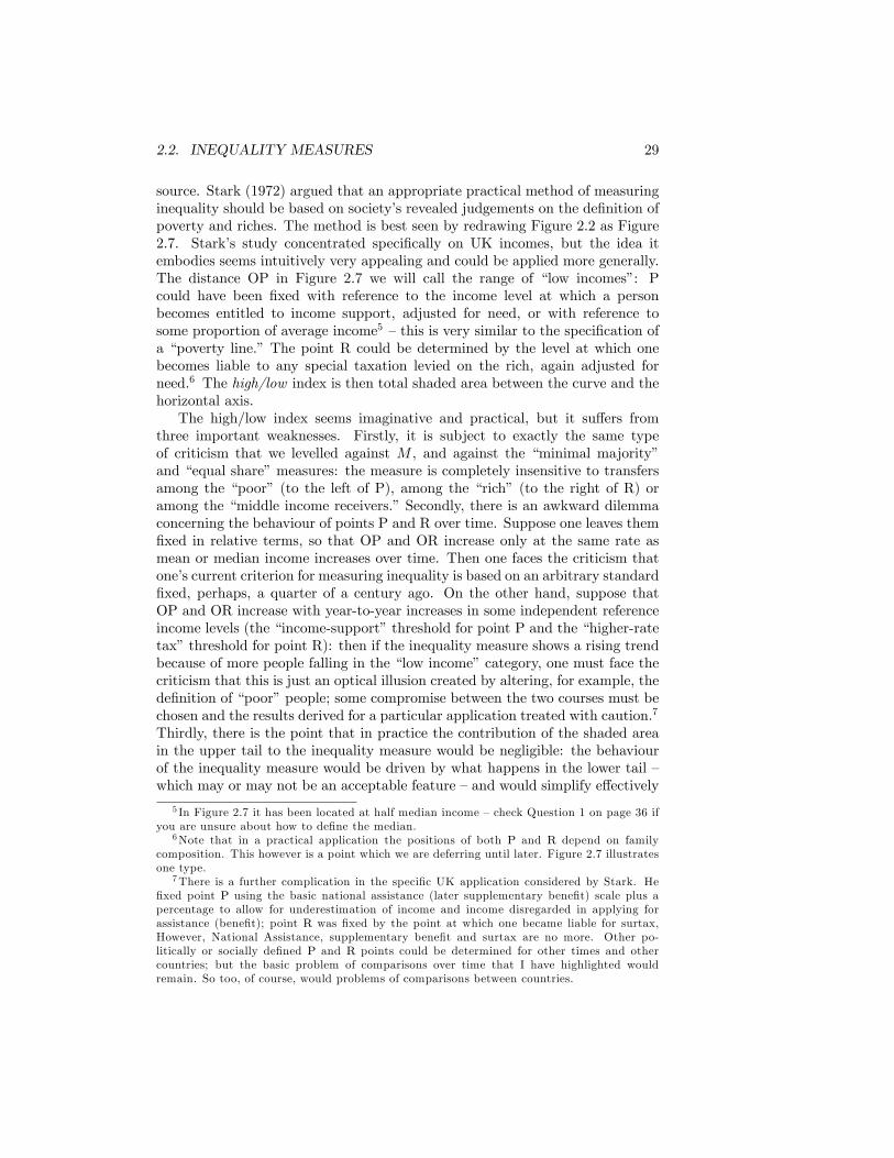
2.2. INEQUALITY MEASURES 29
source. Stark (1972) argued that an appropriate practical method of measuringinequality should be based on society�s revealed judgements on the de�nition ofpoverty and riches. The method is best seen by redrawing Figure 2.2 as Figure2.7. Stark�s study concentrated speci�cally on UK incomes, but the idea itembodies seems intuitively very appealing and could be applied more generally.The distance OP in Figure 2.7 we will call the range of �low incomes�: Pcould have been �xed with reference to the income level at which a personbecomes entitled to income support, adjusted for need, or with reference tosome proportion of average income5 �this is very similar to the speci�cation ofa �poverty line.�The point R could be determined by the level at which onebecomes liable to any special taxation levied on the rich, again adjusted forneed.6 The high/low index is then total shaded area between the curve and thehorizontal axis.The high/low index seems imaginative and practical, but it su¤ers from
three important weaknesses. Firstly, it is subject to exactly the same typeof criticism that we levelled against M , and against the �minimal majority�and �equal share�measures: the measure is completely insensitive to transfersamong the �poor� (to the left of P), among the �rich� (to the right of R) oramong the �middle income receivers.�Secondly, there is an awkward dilemmaconcerning the behaviour of points P and R over time. Suppose one leaves them�xed in relative terms, so that OP and OR increase only at the same rate asmean or median income increases over time. Then one faces the criticism thatone�s current criterion for measuring inequality is based on an arbitrary standard�xed, perhaps, a quarter of a century ago. On the other hand, suppose thatOP and OR increase with year-to-year increases in some independent referenceincome levels (the �income-support�threshold for point P and the �higher-ratetax�threshold for point R): then if the inequality measure shows a rising trendbecause of more people falling in the �low income�category, one must face thecriticism that this is just an optical illusion created by altering, for example, thede�nition of �poor�people; some compromise between the two courses must bechosen and the results derived for a particular application treated with caution.7
Thirdly, there is the point that in practice the contribution of the shaded areain the upper tail to the inequality measure would be negligible: the behaviourof the inequality measure would be driven by what happens in the lower tail �which may or may not be an acceptable feature �and would simplify e¤ectively
5 In Figure 2.7 it has been located at half median income �check Question 1 on page 36 ifyou are unsure about how to de�ne the median.
6Note that in a practical application the positions of both P and R depend on familycomposition. This however is a point which we are deferring until later. Figure 2.7 illustratesone type.
7There is a further complication in the speci�c UK application considered by Stark. He�xed point P using the basic national assistance (later supplementary bene�t) scale plus apercentage to allow for underestimation of income and income disregarded in applying forassistance (bene�t); point R was �xed by the point at which one became liable for surtax,However, National Assistance, supplementary bene�t and surtax are no more. Other po-litically or socially de�ned P and R points could be determined for other times and othercountries; but the basic problem of comparisons over time that I have highlighted wouldremain. So too, of course, would problems of comparisons between countries.
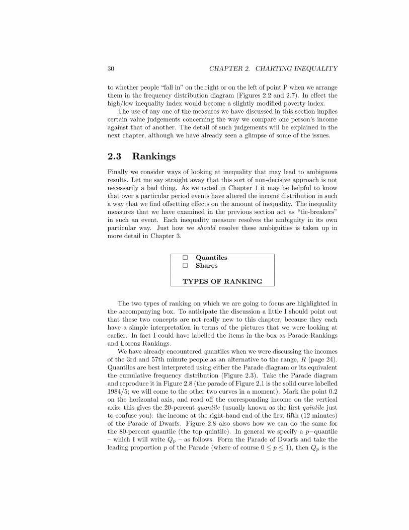
30 CHAPTER 2. CHARTING INEQUALITY
to whether people �fall in�on the right or on the left of point P when we arrangethem in the frequency distribution diagram (Figures 2.2 and 2.7). In e¤ect thehigh/low inequality index would become a slightly modi�ed poverty index.The use of any one of the measures we have discussed in this section implies
certain value judgements concerning the way we compare one person�s incomeagainst that of another. The detail of such judgements will be explained in thenext chapter, although we have already seen a glimpse of some of the issues.
2.3 Rankings
Finally we consider ways of looking at inequality that may lead to ambiguousresults. Let me say straight away that this sort of non-decisive approach is notnecessarily a bad thing. As we noted in Chapter 1 it may be helpful to knowthat over a particular period events have altered the income distribution in sucha way that we �nd o¤setting e¤ects on the amount of inequality. The inequalitymeasures that we have examined in the previous section act as �tie-breakers�in such an event. Each inequality measure resolves the ambiguity in its ownparticular way. Just how we should resolve these ambiguities is taken up inmore detail in Chapter 3.
� Quantiles� Shares
TYPES OF RANKING
The two types of ranking on which we are going to focus are highlighted inthe accompanying box. To anticipate the discussion a little I should point outthat these two concepts are not really new to this chapter, because they eachhave a simple interpretation in terms of the pictures that we were looking atearlier. In fact I could have labelled the items in the box as Parade Rankingsand Lorenz Rankings.We have already encountered quantiles when we were discussing the incomes
of the 3rd and 57th minute people as an alternative to the range, R (page 24).Quantiles are best interpreted using either the Parade diagram or its equivalentthe cumulative frequency distribution (Figure 2.3). Take the Parade diagramand reproduce it in Figure 2.8 (the parade of Figure 2.1 is the solid curve labelled1984/5; we will come to the other two curves in a moment). Mark the point 0:2on the horizontal axis, and read o¤ the corresponding income on the verticalaxis: this gives the 20-percent quantile (usually known as the �rst quintile justto confuse you): the income at the right-hand end of the �rst �fth (12 minutes)of the Parade of Dwarfs. Figure 2.8 also shows how we can do the same forthe 80-percent quantile (the top quintile). In general we specify a p�quantile�which I will write Qp �as follows. Form the Parade of Dwarfs and take theleading proportion p of the Parade (where of course 0 � p � 1), then Qp is the
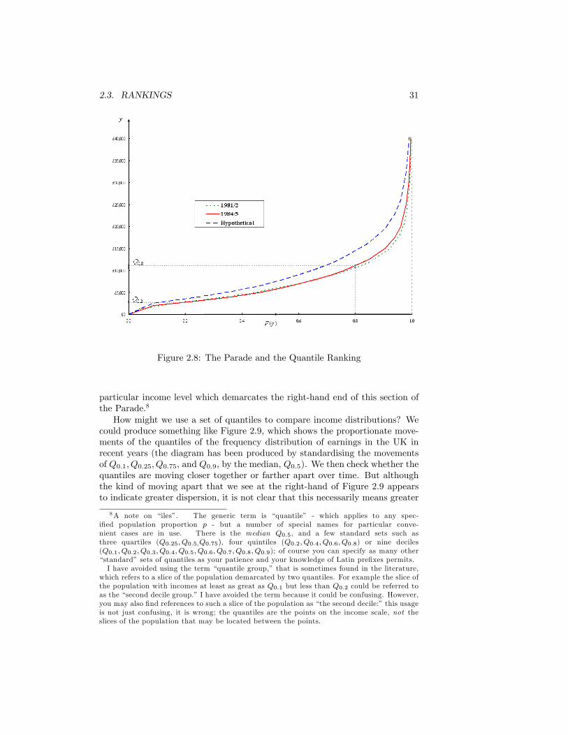
2.3. RANKINGS 31
Figure 2.8: The Parade and the Quantile Ranking
particular income level which demarcates the right-hand end of this section ofthe Parade.8
How might we use a set of quantiles to compare income distributions? Wecould produce something like Figure 2.9, which shows the proportionate move-ments of the quantiles of the frequency distribution of earnings in the UK inrecent years (the diagram has been produced by standardising the movementsof Q0:1; Q0:25; Q0:75, and Q0:9, by the median, Q0:5). We then check whether thequantiles are moving closer together or farther apart over time. But althoughthe kind of moving apart that we see at the right-hand of Figure 2.9 appearsto indicate greater dispersion, it is not clear that this necessarily means greater
8A note on �iles�. The generic term is �quantile� - which applies to any spec-i�ed population proportion p - but a number of special names for particular conve-nient cases are in use. There is the median Q0:5, and a few standard sets such asthree quartiles (Q0:25; Q0:5;Q0:75), four quintiles (Q0:2; Q0:4; Q0:6; Q0:8) or nine deciles(Q0:1; Q0:2; Q0:3; Q0:4; Q0:5; Q0:6; Q0:7; Q0:8; Q0:9); of course you can specify as many other�standard� sets of quantiles as your patience and your knowledge of Latin pre�xes permits.I have avoided using the term �quantile group,� that is sometimes found in the literature,
which refers to a slice of the population demarcated by two quantiles. For example the slice ofthe population with incomes at least as great as Q0:1 but less than Q0:2 could be referred toas the �second decile group.�I have avoided the term because it could be confusing. However,you may also �nd references to such a slice of the population as �the second decile:�this usageis not just confusing, it is wrong; the quantiles are the points on the income scale, not theslices of the population that may be located between the points.
32 CHAPTER 2. CHARTING INEQUALITY
Figure 2.9: Quantile ratios of earnings of adult men, UK 1968-2007. Source:Annual Survey of Hours and Earnings
inequality: the movement of the corresponding income shares (which we discussin a moment) could in principle be telling us a di¤erent story.9
However, we might also be interested in the simple quantile ranking of thedistributions, which focuses on the absolute values of the quantiles, rather thanquantile ratios. For example, suppose that over time all the quantiles of thedistribution increase by 30 percent as shown by the curve labelled �hypothetical�in Figure 2.8 (in the jargon we then say that according to the quantile rankingthe new distribution dominates the old one). Then we might say �there are stilllots of dwarfs about�, to which the reply might be �yes but at least everybody isa bit taller.�Even if we cannot be speci�c about whether this means that thereis more or less inequality as a result, the phenomenon of a clear quantile rankingis telling us something interesting about the income distribution which we willdiscuss more in the next chapter. On the other hand if we were to compare1981/2 and 1984/5 in Figure 2.8 we would have to admit that over the threeyear period the giants became a little taller (Q0:8 increased slightly), but thedwarfs became even shorter (Q0:2 decreased slightly): the 1984/5 distributiondoes not dominate that for 1981/2.
9 In case this is not obvious consider a population with just 8 people in it; in year A theincome distribution is (2; 3; 3; 4; 5; 6; 6; 7), and it is fairly obvious that Q0:25 = 3 and Q0:75 = 6in year B the distribution becomes (0; 4; 4; 4; 5; 5; 5; 9) and we can see now that Q0:25 = 4 andQ0:75 = 5. Mean income and median income have remained unchanged and the quartileshave narrowed: but has inequality really gone down? The story from the shares suggestsotherwise: the share of the bottom 25% has actually fallen (from 5=36 to 4=36) and the shareof the top 25% has risen (from 13=36 to 14=36).
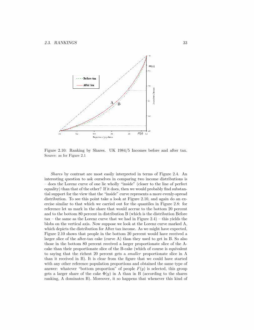
2.3. RANKINGS 33
Figure 2.10: Ranking by Shares. UK 1984/5 Incomes before and after tax.Source: as for Figure 2.1
Shares by contrast are most easily interpreted in terms of Figure 2.4. Aninteresting question to ask ourselves in comparing two income distributions is�does the Lorenz curve of one lie wholly �inside�(closer to the line of perfectequality) than that of the other? If it does, then we would probably �nd substan-tial support for the view that the �inside�curve represents a more evenly-spreaddistribution. To see this point take a look at Figure 2.10, and again do an ex-ercise similar to that which we carried out for the quantiles in Figure 2.8: forreference let us mark in the share that would accrue to the bottom 20 percentand to the bottom 80 percent in distribution B (which is the distribution Beforetax �the same as the Lorenz curve that we had in Figure 2.4) �this yields theblobs on the vertical axis. Now suppose we look at the Lorenz curve marked A,which depicts the distribution for After tax income. As we might have expected,Figure 2.10 shows that people in the bottom 20 percent would have received alarger slice of the after-tax cake (curve A) than they used to get in B. So alsothose in the bottom 80 percent received a larger proportionate slice of the A-cake than their proportionate slice of the B-cake (which of course is equivalentto saying that the richest 20 percent gets a smaller proportionate slice in Athan it received in B). It is clear from the �gure that we could have startedwith any other reference population proportions and obtained the same type ofanswer: whatever �bottom proportion� of people F (y) is selected, this groupgets a larger share of the cake �(y) in A than in B (according to the sharesranking, A dominates B). Moreover, it so happens that whenever this kind of
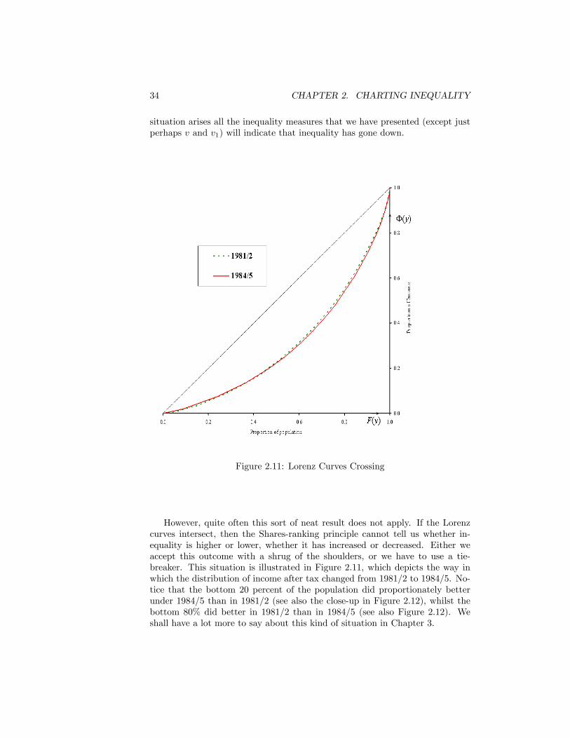
34 CHAPTER 2. CHARTING INEQUALITY
situation arises all the inequality measures that we have presented (except justperhaps v and v1) will indicate that inequality has gone down.
Figure 2.11: Lorenz Curves Crossing
However, quite often this sort of neat result does not apply. If the Lorenzcurves intersect, then the Shares-ranking principle cannot tell us whether in-equality is higher or lower, whether it has increased or decreased. Either weaccept this outcome with a shrug of the shoulders, or we have to use a tie-breaker. This situation is illustrated in Figure 2.11, which depicts the way inwhich the distribution of income after tax changed from 1981/2 to 1984/5. No-tice that the bottom 20 percent of the population did proportionately betterunder 1984/5 than in 1981/2 (see also the close-up in Figure 2.12), whilst thebottom 80% did better in 1981/2 than in 1984/5 (see also Figure 2.12). Weshall have a lot more to say about this kind of situation in Chapter 3.

2.3. RANKINGS 35
Figure 2.12: Change at the bottom of the income distribution
Figure 2.13: Change at the top of the income distribution
36 CHAPTER 2. CHARTING INEQUALITY
2.4 From charts to analysis
We have seen how quite a large number of ad hoc inequality measures are as-sociated with various diagrams that chart inequality, which are themselves in-terlinked. But however appealing each of these pictorial representations mightbe, we seem to �nd important reservations about any of the associated inequal-ity measures. Perhaps the most unsatisfactory aspect of all of these indices isthat the basis for using them is indeed ad hoc: the rationale for using themwas based on intuition and a little graphical serendipity. What we really needis proper theoretical basis for comparing income distributions and for decidingwhat constitutes a �good�inequality measure.This is where the ranking techniques that we have been considering come in
particularly useful. Although they are indecisive in themselves, they yet providea valuable introduction to the deeper analysis of inequality measurement to befound in the next chapter.
2.5 Questions
1. Explain how to represent median income in Pen�s Parade. How would yourepresent the upper and lower quartiles? [See footnote 8.]
2. Describe how the following would look:
(a) Pen�s Parade with negative incomes.
(b) The Lorenz curve if there were some individuals with negative in-comes but mean income were still positive.
(c) The Lorenz curve if there were so many individuals with negativeincomes that mean income itself were negative. [See the TechnicalAppendix, page 166. for more on this.]
3. DeNavas-Walt et al. (2008) presents a convenient summary of UnitedStates�income distribution data based on the Annual Social and EconomicSupplement to the 2008 Current Population Survey. (a) How would theinformation in their Table A-1 need to be adapted in order to producecharts similar to Figure 2.2? (b) Use the information in Table A-3 toconstruct Pen�s Parade for 1967, 1987, 2007: how does the Parade appearto have shifted over 40 years? (c) Use the information in Table A-3 toconstruct the Lorenz curves for 1967, 1987, 2007: what has happened toinequality over the period? [Document is available on-line using the linkon the website http://darp.lse.ac.uk/MI3]
4. Reconstruct the histogram for the UK 1984/5, before-tax income, usingthe �le �ET income distribution� on the website (see the Technical Ap-pendix page 174 for guidance on how to use the �le). Now merge adja-cent pairs of intervals (so that, for example the intervals [£ 0,£ 2000] and
2.5. QUESTIONS 37
[£ 2000,£ 3000] become [£ 0,£ 3000]) and redraw the histogram: commenton your �ndings.
5. Using the same data source for the UK 1984/5, before-tax income, con-struct the distribution function corresponding to the histogram drawn inquestion 4. Now, instead of assuming that the distribution of income fol-lows the histogram shape, assume that within each income interval allincome receivers get the mean income of that interval. Again draw thedistribution function. Why does it look like a �ight of steps?
6. Suppose a country�s tax and bene�t system operates so that taxes payableare determined by the formula
t[y � y0]
where y is the person�s original (pre-tax) income, t is the marginal taxrate and y0 is a threshold income. Persons with incomes below y0 receivea net payment from the government (�negative tax�). If the distributionof original income is y1; y2; :::; yn, use the formulas given in the TechnicalAppendix (page 151) to write down the coe¢ cient of variation and theGini coe¢ cient for after-tax income. Comment on your results.
7. Suppose the income distribution before tax is represented by a set of num-bers fy(1); y(2); :::; y(n)g, where y(1) � y(2) � y(3):::. Write down an expres-sion for the Lorenz curve. If the tax system were to be of the form givenin question 6, what would be the Lorenz curve of disposable (after tax)income? Will it lie above the Lorenz curve for original income? [For fur-ther discussion of the point here see Jakobsson (1976) and Eichhorn et al.(1984) .]
8.
(a) Ruritania consists of six districts that are approximately of equal sizein terms of population. In 2007 per-capita incomes in the six districtswere:
� Rural ($500, $500, $500)� Urban ($20 000, $28 284, $113 137).
What is mean income for the Rural districts, for the Urban districtsand for the whole of Ruritania. Compute the logarithmic variance,the relative mean deviation and the Gini coe¢ cient for the Ruraldistricts and the Urban districts separately and for the whole of Ru-ritania. (You will �nd that these are easily adapted from the �le�East-West�on the website, and you should ignore any income dif-ferences within any one district.)
(b) By 2008 the per-capita income distribution had changed as follows:
� Rural: ($499, $500, $501)

38 CHAPTER 2. CHARTING INEQUALITY
� Urban: ($21 000, $26 284, $114 137)Rework the computations of part (a) for the 2008 data. Did inequal-ity rise or fall between 2007 and 2008? [See the discussion on page64 below for an explanation of this phenomenon.]
Chapter 3
Analysing Inequality
�He�s half a millionaire: he has the air but not the million.� �Jewish Proverb
In Chapter 2 we looked at measures of inequality that came about moreor less by accident. In some cases a concept was borrowed from statistics andpressed into service as a tool of inequality measurement. In others a useful dia-grammatic device was used to generate a measure of inequality that �naturally�seemed to �t it, the relative mean deviation and the Parade, for example; orthe Gini coe¢ cient and the Lorenz curve.
� Social Welfare� Information Theory� Structural Approach
APPROACHES TO INEQUALITY ANALYSIS
However, if we were to follow the austere and analytical course of rejectingvisual intuition, and of constructing an inequality measure from ��rst princi-ples�, what approach should we adopt? I shall outline three approaches, andin doing so consider mainly special cases that illustrate the essential points eas-ily without pretending to be analytically rigorous. The �rst method we shallexamine is that of making inequality judgments from and deriving inequalitymeasures from social-welfare functions. The social welfare function itself maybe supposed to subsume values of society regarding equality and justice, andthus the derived inequality measures are given a normative basis. The secondmethod is to see the quanti�cation of inequality as an o¤shoot of the problem ofcomparing probability distributions: to do this we draw upon a fruitful analogywith information theory. The �nal �structural �approach is to specify a setof principles or axioms su¢ cient to determine an inequality measure uniquely;
39
40 CHAPTER 3. ANALYSING INEQUALITY
the choice of axioms themselves, of course, will be determined by what we thinkan inequality measure �should�look like. Each of these approaches raises somebasic questions about the meaning and interpretation of inequality.
3.1 Social-welfare functions
One way of introducing social values concerning inequality is to use a social-welfare function (SWF) which simply ranks all the possible states of societyin the order of (society�s) preference. The various �states� could be functionsof all sorts of things �personal income, wealth, size of people�s cars �but weusually attempt to isolate certain characteristics which are considered �relevant�in situations of social choice. We do not have to concern ourselves here with themeans by which this social ranking is derived. The ranking may be handed downby parliament, imposed by a dictator, suggested by the trade unions, or simplythought up by the observing economist �the key point is that its characteristicsare carefully speci�ed in advance, and that these characteristics can be criticisedon their own merits.In its simplest form, a social-welfare function simply orders social states
unambiguously: if state A is preferable to state B then, and only then, the SWFhas a higher value for state A than that for state B. How may we construct auseful SWF? To help in answering this question I shall list some properties thatit may be desirable for the SWF to possess; we shall be examining their economicsigni�cance later. First let me introduce a preliminary piece of notation: let yiAbe the magnitude of person i�s �economic position� in social state A, where iis a label that can be any number between 1 and n inclusive. For example, yiAcould be the income of Mr Jones of Potter�s Bar in the year 1984. Where itdoes not matter, the A-su¢ x will be dropped.Now let us use this device to specify �ve characteristics of the SWF. The
�rst three are as follows:
� The SWF is individualistic and nondecreasing, if the welfare level in anystate A, denoted by a number WA, can be written:
WA =W (y1A; y2A; :::; ynA):
and, if yiB � yiA for all i implies, ceteris paribus, that WB � WA, whichin turn implies that state B is at least as good as state A.
� The SWF is symmetric if it is true that, for any state,
W (y1; y2; :::; yn) =W (y2; y1; :::; yn) = ::: =W (yn; y2; :::; y1);
This means that the function W treats individual incomes anonymously:the value of W does not depend on the particular assignment of labels tomembers of the population.

3.1. SOCIAL-WELFARE FUNCTIONS 41
� The SWF is additive if it can be written
W (y1; y2; :::; yn) =nXi=1
Ui(yi) = U1(y1) + U2(y2) + :::+ Un(yn); (3.1)
where U1 is a function of y1 alone, and so on.
If these three properties are all satis�ed then we can write the SWF like this:
W (y1; y2; :::; yn) =nXi=1
U(yi) = U(y1) + U(y2) + :::+ U(yn); (3.2)
where U is the same function for each person and where U(yi) increases with yi.If we restrict attention to this special case the de�nitions of the remaining twoproperties of the SWF can be simpli�ed, since they may be expressed in termsof the function U alone. Let us call U(y1) the social utility of, or the welfareindex for, person 1. The rate at which this index increases is
U 0(y1) =dU(y1)
d y1;
which can be thought of as the social marginal utility of, or the welfare weight,for person 1. Notice that, because of the �rst property, none of the welfareweights can be negative. Then properties 4 and 5 are:
� The SWF is strictly concave if the welfare weight always decreases as yiincreases.
� The SWF has constant elasticity, or constant relative inequality aversionif U(yi) can be written
U(yi) =y1�"i � 11� " (3.3)
(or in a cardinally equivalent form), where " is the inequality aversionparameter, which is non-negative.1
I must emphasise that this is a very abbreviated discussion of the propertiesof SWFs. However, these �ve basic properties �or assumptions about the SWF� are su¢ cient to derive a convenient purpose-built inequality measure, andthus we shall examine their signi�cance more closely.The �rst of the �ve properties simply states that the welfare numbers should
be related to individual incomes (or wealth, etc.) so that if any person�s incomegoes up social welfare cannot go down. The term �individualistic� may be
1Notice that I have used a slightly di¤erent cardinalisation of U from that employed in the�rst edition (1977) of this book in order to make the presentation of �gures a little clearer.This change does not a¤ect any of the results.
42 CHAPTER 3. ANALYSING INEQUALITY
applied to the case where the SWF is de�ned in relation to the satisfactionspeople derive from their income, rather than the incomes themselves. I shallignore this point and assume that any standardisation of the incomes, yi, (forexample to allow for di¤ering needs) has already been performed.2 This per-mits a straightforward comparison of the individual levels, and of di¤erences inindividual levels, of people�s �economic position��represented by the yi andloosely called �income.� The idea that welfare is non-decreasing in income isperhaps not as innocuous as it �rst seems: it rules out for example the ideathat if one disgustingly rich person gets richer still whilst everyone else�s incomestays the same, the e¤ect on inequality is so awful that social welfare actuallygoes down.Given that we treat these standardised incomes yi as a measure that puts
everyone in the population on an equal footing as regards needs and desert, thesecond property (symmetry) naturally follows �there is no reason why welfareshould be higher or lower if any two people simply swapped incomes.The third assumption is quite strong, and is independent of the second.
Suppose you measure WB�WA, the increase in welfare from state A to state B,where the only change is an increase in person 1�s income from £ 20 000 to £ 21000. Then the additivity assumption states that the e¤ect of this change alone(increasing person 1�s income from £ 20 000 to £ 21 000) is quite independentof what the rest of state A looked like � it does not matter whether everyoneelse had £ 1 or £ 100 000, WB �WA is just the same for this particular change.However, this convenient assumption is not as restrictive in terms of the resultinginequality measures as it might seem at �rst sight �this will become clearer whenwe consider the concept of �distance�between income shares later.We could have phrased the strict concavity assumption in much more general
terms, but the discussion is easier in terms of the welfare index U . Note thatthis is not an ordinary utility function (such as might be used to characterisethe bene�t that an individual gets from his income), although it may have verysimilar properties: it represents the valuation given by society of a person�sincome. One may think of this as a �social utility function.� In this case,the concept corresponding to �social marginal utility� is the quantity U 0(yi)which we have called the welfare weight. The reason for the latter term is asfollows. Consider a government programme which brings about a (small) changein everyone�s income: 4y1;4y2; :::;4yn. What is the change in social welfare?It is simply
dW = U 0(y1)4y1 + U 0(y2)4y2 + :::+ U 0(yn)4yn;
so the U 0-quantities act as a system of weights when summing the e¤ects ofthe programme over the whole population. How should the weights be �xed?The strict concavity assumption tells us that the higher a person�s income, thelower the social weight he is given. If we are averse to inequality this seems
2Once again notice my loose use of the word �person�. In practice incomes may bereceived by households or families of di¤ering sizes, in which case yi must be reinterpreted as�equivalised� incomes: see page 105 for more on this.
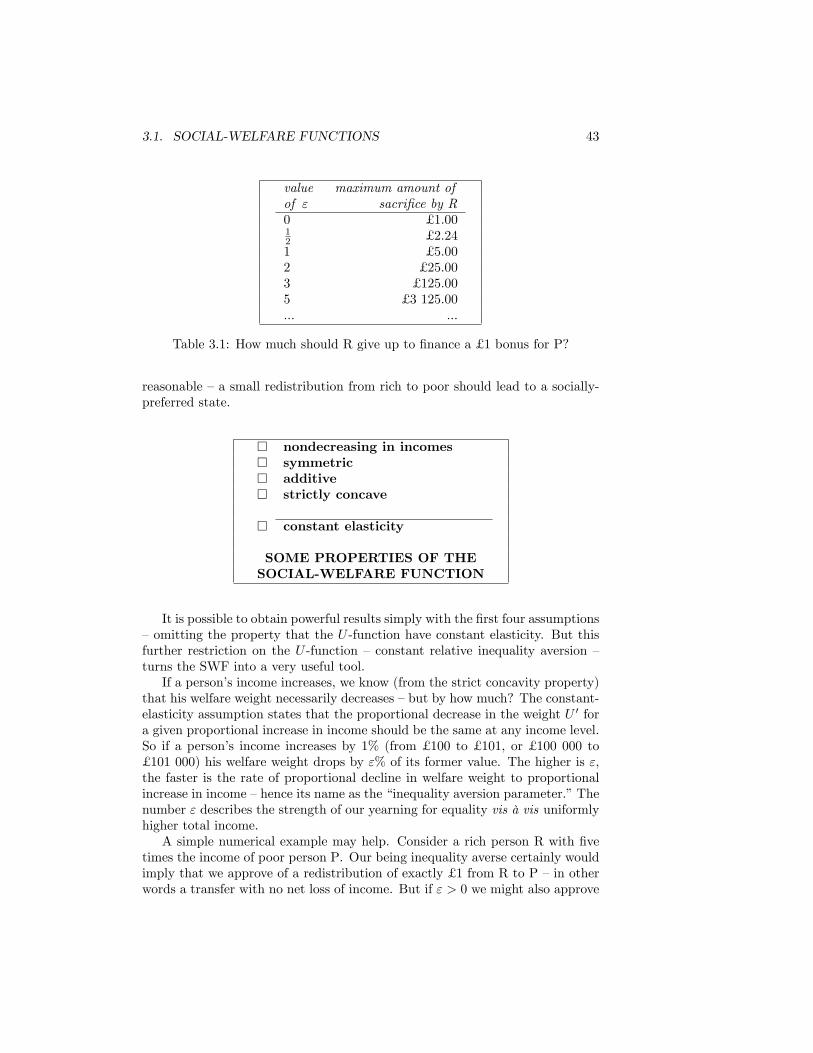
3.1. SOCIAL-WELFARE FUNCTIONS 43
value maximum amount ofof " sacri�ce by R0 £ 1.0012 £ 2.241 £ 5.002 £ 25.003 £ 125.005 £ 3 125.00... ...
Table 3.1: How much should R give up to �nance a £ 1 bonus for P?
reasonable �a small redistribution from rich to poor should lead to a socially-preferred state.
� nondecreasing in incomes� symmetric� additive� strictly concave
� constant elasticity
SOME PROPERTIES OF THESOCIAL-WELFARE FUNCTION
It is possible to obtain powerful results simply with the �rst four assumptions�omitting the property that the U -function have constant elasticity. But thisfurther restriction on the U -function � constant relative inequality aversion �turns the SWF into a very useful tool.If a person�s income increases, we know (from the strict concavity property)
that his welfare weight necessarily decreases �but by how much? The constant-elasticity assumption states that the proportional decrease in the weight U 0 fora given proportional increase in income should be the same at any income level.So if a person�s income increases by 1% (from £ 100 to £ 101, or £ 100 000 to£ 101 000) his welfare weight drops by "% of its former value. The higher is ",the faster is the rate of proportional decline in welfare weight to proportionalincrease in income �hence its name as the �inequality aversion parameter.�Thenumber " describes the strength of our yearning for equality vis à vis uniformlyhigher total income.A simple numerical example may help. Consider a rich person R with �ve
times the income of poor person P. Our being inequality averse certainly wouldimply that we approve of a redistribution of exactly £ 1 from R to P �in otherwords a transfer with no net loss of income. But if " > 0 we might also approve
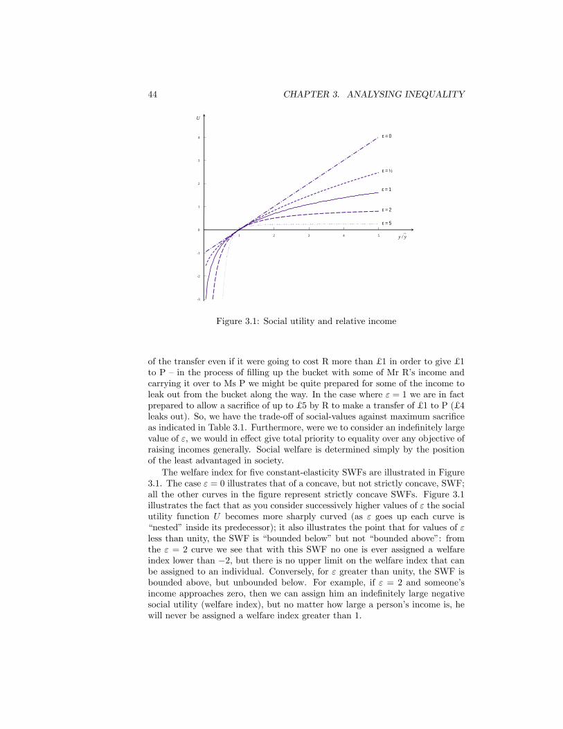
44 CHAPTER 3. ANALYSING INEQUALITY
1 2 3 4 5
3
2
1
0
1
2
3
4
ε = ½
ε = 0
ε = 1
ε = 2
ε = 5
y / y_
U
Figure 3.1: Social utility and relative income
of the transfer even if it were going to cost R more than £ 1 in order to give £ 1to P �in the process of �lling up the bucket with some of Mr R�s income andcarrying it over to Ms P we might be quite prepared for some of the income toleak out from the bucket along the way. In the case where " = 1 we are in factprepared to allow a sacri�ce of up to £ 5 by R to make a transfer of £ 1 to P (£ 4leaks out). So, we have the trade-o¤ of social-values against maximum sacri�ceas indicated in Table 3.1. Furthermore, were we to consider an inde�nitely largevalue of ", we would in e¤ect give total priority to equality over any objective ofraising incomes generally. Social welfare is determined simply by the positionof the least advantaged in society.The welfare index for �ve constant-elasticity SWFs are illustrated in Figure
3.1. The case " = 0 illustrates that of a concave, but not strictly concave, SWF;all the other curves in the �gure represent strictly concave SWFs. Figure 3.1illustrates the fact that as you consider successively higher values of " the socialutility function U becomes more sharply curved (as " goes up each curve is�nested�inside its predecessor); it also illustrates the point that for values of "less than unity, the SWF is �bounded below�but not �bounded above�: fromthe " = 2 curve we see that with this SWF no one is ever assigned a welfareindex lower than �2, but there is no upper limit on the welfare index that canbe assigned to an individual. Conversely, for " greater than unity, the SWF isbounded above, but unbounded below. For example, if " = 2 and someone�sincome approaches zero, then we can assign him an inde�nitely large negativesocial utility (welfare index), but no matter how large a person�s income is, hewill never be assigned a welfare index greater than 1.
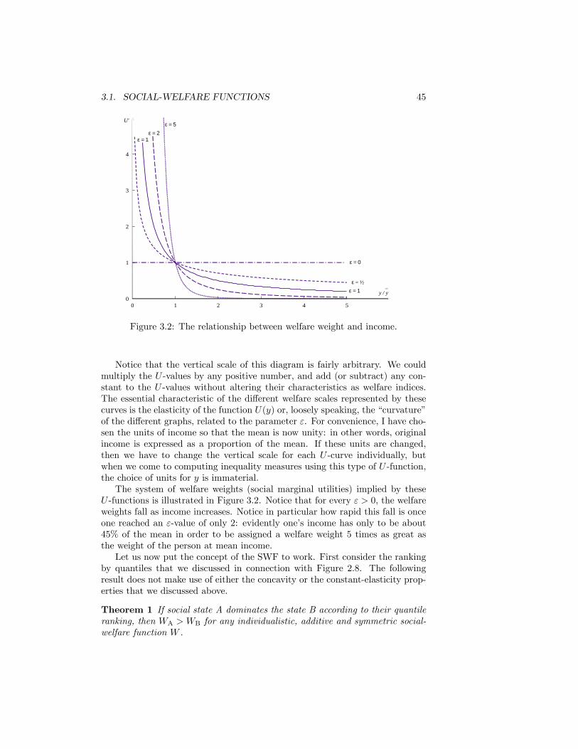
3.1. SOCIAL-WELFARE FUNCTIONS 45
0 1 2 3 4 50
1
2
3
4
ε = 1ε = 2
ε = 5U'
y / y_
ε = 1
ε = 0
ε = ½
Figure 3.2: The relationship between welfare weight and income.
Notice that the vertical scale of this diagram is fairly arbitrary. We couldmultiply the U -values by any positive number, and add (or subtract) any con-stant to the U -values without altering their characteristics as welfare indices.The essential characteristic of the di¤erent welfare scales represented by thesecurves is the elasticity of the function U(y) or, loosely speaking, the �curvature�of the di¤erent graphs, related to the parameter ". For convenience, I have cho-sen the units of income so that the mean is now unity: in other words, originalincome is expressed as a proportion of the mean. If these units are changed,then we have to change the vertical scale for each U -curve individually, butwhen we come to computing inequality measures using this type of U -function,the choice of units for y is immaterial.The system of welfare weights (social marginal utilities) implied by these
U -functions is illustrated in Figure 3.2. Notice that for every " > 0, the welfareweights fall as income increases. Notice in particular how rapid this fall is onceone reached an "-value of only 2: evidently one�s income has only to be about45% of the mean in order to be assigned a welfare weight 5 times as great asthe weight of the person at mean income.Let us now put the concept of the SWF to work. First consider the ranking
by quantiles that we discussed in connection with Figure 2.8. The followingresult does not make use of either the concavity or the constant-elasticity prop-erties that we discussed above.
Theorem 1 If social state A dominates the state B according to their quantileranking, then WA > WB for any individualistic, additive and symmetric social-welfare function W .
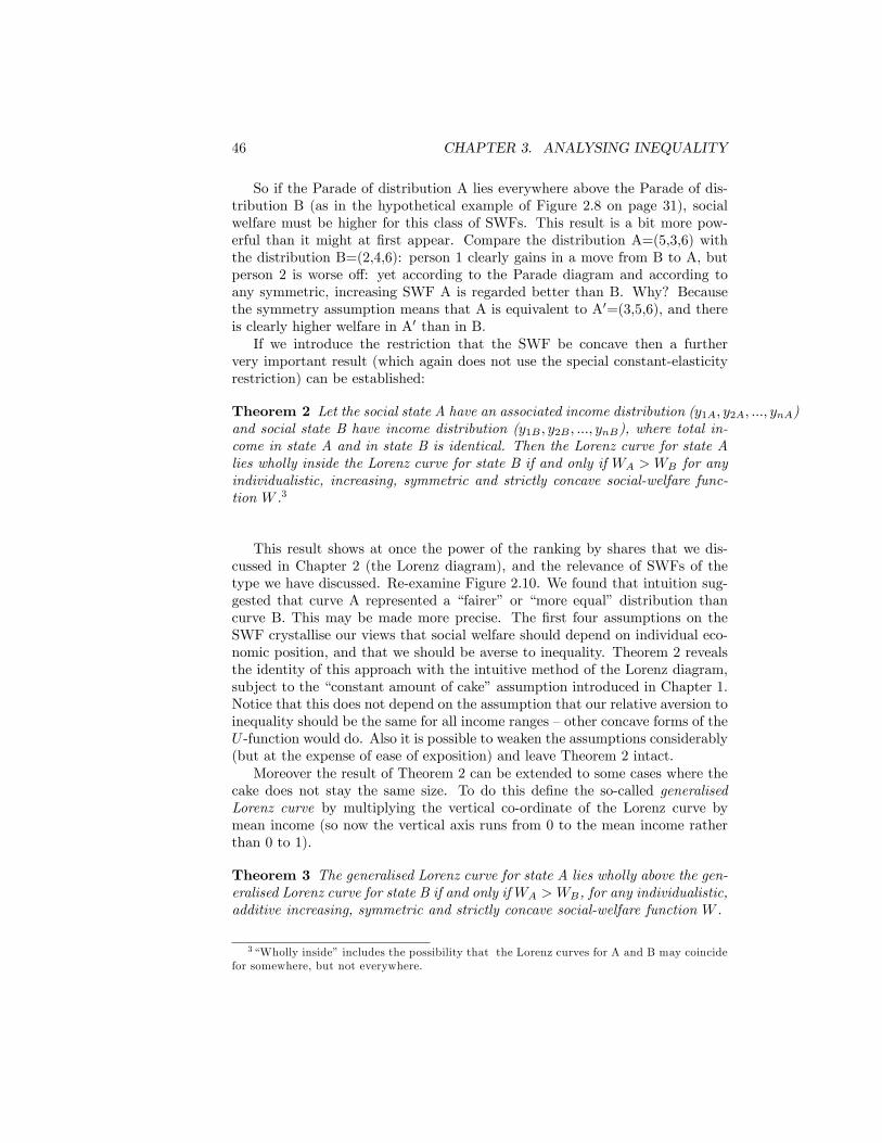
46 CHAPTER 3. ANALYSING INEQUALITY
So if the Parade of distribution A lies everywhere above the Parade of dis-tribution B (as in the hypothetical example of Figure 2.8 on page 31), socialwelfare must be higher for this class of SWFs. This result is a bit more pow-erful than it might at �rst appear. Compare the distribution A=(5,3,6) withthe distribution B=(2,4,6): person 1 clearly gains in a move from B to A, butperson 2 is worse o¤: yet according to the Parade diagram and according toany symmetric, increasing SWF A is regarded better than B. Why? Becausethe symmetry assumption means that A is equivalent to A0=(3,5,6), and thereis clearly higher welfare in A0 than in B.If we introduce the restriction that the SWF be concave then a further
very important result (which again does not use the special constant-elasticityrestriction) can be established:
Theorem 2 Let the social state A have an associated income distribution (y1A; y2A; :::; ynA)and social state B have income distribution (y1B ; y2B ; :::; ynB), where total in-come in state A and in state B is identical. Then the Lorenz curve for state Alies wholly inside the Lorenz curve for state B if and only if WA > WB for anyindividualistic, increasing, symmetric and strictly concave social-welfare func-tion W .3
This result shows at once the power of the ranking by shares that we dis-cussed in Chapter 2 (the Lorenz diagram), and the relevance of SWFs of thetype we have discussed. Re-examine Figure 2.10. We found that intuition sug-gested that curve A represented a �fairer� or �more equal� distribution thancurve B. This may be made more precise. The �rst four assumptions on theSWF crystallise our views that social welfare should depend on individual eco-nomic position, and that we should be averse to inequality. Theorem 2 revealsthe identity of this approach with the intuitive method of the Lorenz diagram,subject to the �constant amount of cake�assumption introduced in Chapter 1.Notice that this does not depend on the assumption that our relative aversion toinequality should be the same for all income ranges �other concave forms of theU -function would do. Also it is possible to weaken the assumptions considerably(but at the expense of ease of exposition) and leave Theorem 2 intact.Moreover the result of Theorem 2 can be extended to some cases where the
cake does not stay the same size. To do this de�ne the so-called generalisedLorenz curve by multiplying the vertical co-ordinate of the Lorenz curve bymean income (so now the vertical axis runs from 0 to the mean income ratherthan 0 to 1).
Theorem 3 The generalised Lorenz curve for state A lies wholly above the gen-eralised Lorenz curve for state B if and only ifWA > WB, for any individualistic,additive increasing, symmetric and strictly concave social-welfare function W .
3�Wholly inside�includes the possibility that the Lorenz curves for A and B may coincidefor somewhere, but not everywhere.
3.1. SOCIAL-WELFARE FUNCTIONS 47
Figure 3.3: The Generalised Lorenz Curve Comparison: UK income before tax
For example, we noted in Chapter 2 that the simple shares-ranking criterionwas inconclusive when comparing the distribution of income after tax in the UK,1981/2 with that for the period 1984/5: the ordinary Lorenz curves intersect(see Figures 2.11-2.13). Now let us consider the generalised Lorenz curves forthe same two datasets, which are depicted in Figure 3.3. Notice that the verticalaxes is measured in monetary units, by contrast with that for Figures 2.4 and2.10-2.13; notice also that this method of comparing distributions implies a kindof priority ranking for the mean: as is evident from Figure 3.3 if the mean ofdistribution A is higher than the distribution B, then the generalised Lorenzcurve of B cannot lie above that of A no matter how unequal A may be. So,without further ado, we can assert that any SWF that is additive, individualisticand concave will suggest that social welfare was higher in 1984/5 than in 1981/2.
However, although Theorems 1 to 3 provide us with some fundamental in-sights on the welfare and inequality rankings that may be inferred from incomedistributions, they are limited in two ways.
First, the results are cast exclusively within the context of social welfareanalysis. That is not necessarily a drawback, since the particular welfare criteriathat we have discussed may have considerable intuitive appeal. Nevertheless you
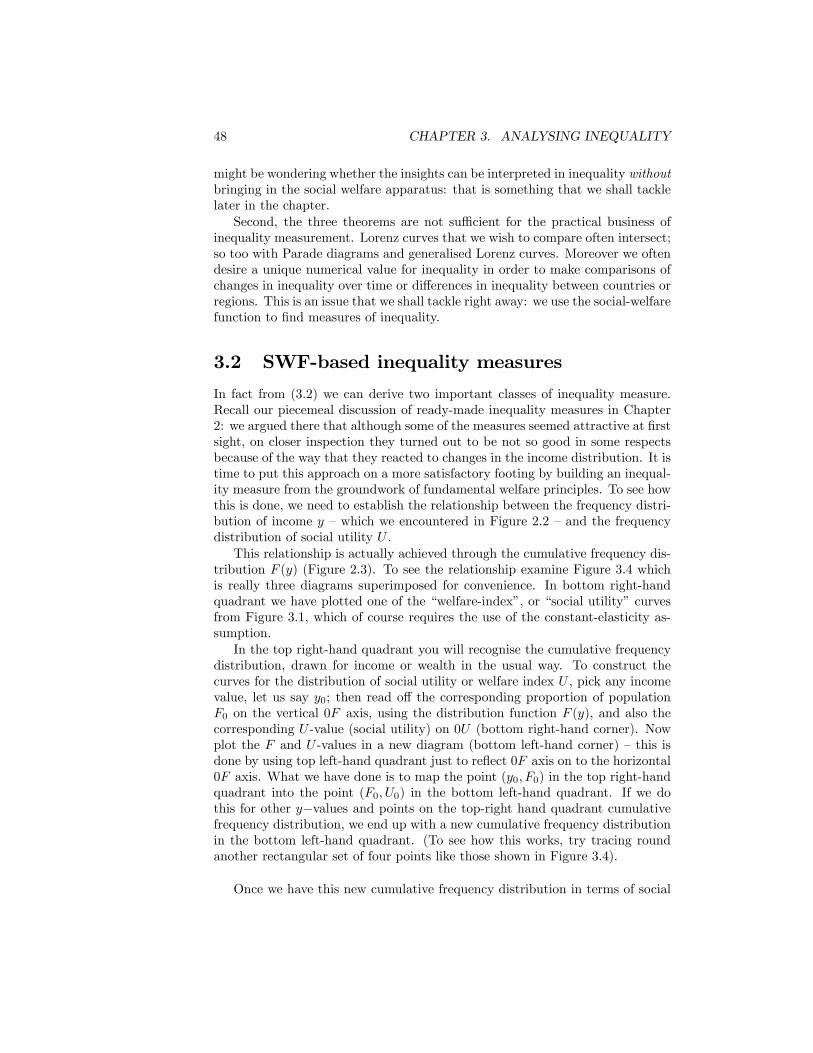
48 CHAPTER 3. ANALYSING INEQUALITY
might be wondering whether the insights can be interpreted in inequality withoutbringing in the social welfare apparatus: that is something that we shall tacklelater in the chapter.Second, the three theorems are not su¢ cient for the practical business of
inequality measurement. Lorenz curves that we wish to compare often intersect;so too with Parade diagrams and generalised Lorenz curves. Moreover we oftendesire a unique numerical value for inequality in order to make comparisons ofchanges in inequality over time or di¤erences in inequality between countries orregions. This is an issue that we shall tackle right away: we use the social-welfarefunction to �nd measures of inequality.
3.2 SWF-based inequality measures
In fact from (3.2) we can derive two important classes of inequality measure.Recall our piecemeal discussion of ready-made inequality measures in Chapter2: we argued there that although some of the measures seemed attractive at �rstsight, on closer inspection they turned out to be not so good in some respectsbecause of the way that they reacted to changes in the income distribution. It istime to put this approach on a more satisfactory footing by building an inequal-ity measure from the groundwork of fundamental welfare principles. To see howthis is done, we need to establish the relationship between the frequency distri-bution of income y �which we encountered in Figure 2.2 �and the frequencydistribution of social utility U .This relationship is actually achieved through the cumulative frequency dis-
tribution F (y) (Figure 2.3). To see the relationship examine Figure 3.4 whichis really three diagrams superimposed for convenience. In bottom right-handquadrant we have plotted one of the �welfare-index�, or �social utility�curvesfrom Figure 3.1, which of course requires the use of the constant-elasticity as-sumption.In the top right-hand quadrant you will recognise the cumulative frequency
distribution, drawn for income or wealth in the usual way. To construct thecurves for the distribution of social utility or welfare index U , pick any incomevalue, let us say y0; then read o¤ the corresponding proportion of populationF0 on the vertical 0F axis, using the distribution function F (y), and also thecorresponding U -value (social utility) on 0U (bottom right-hand corner). Nowplot the F and U -values in a new diagram (bottom left-hand corner) �this isdone by using top left-hand quadrant just to re�ect 0F axis on to the horizontal0F axis. What we have done is to map the point (y0; F0) in the top right-handquadrant into the point (F0; U0) in the bottom left-hand quadrant. If we dothis for other y�values and points on the top-right hand quadrant cumulativefrequency distribution, we end up with a new cumulative frequency distributionin the bottom left-hand quadrant. (To see how this works, try tracing roundanother rectangular set of four points like those shown in Figure 3.4).
Once we have this new cumulative frequency distribution in terms of social
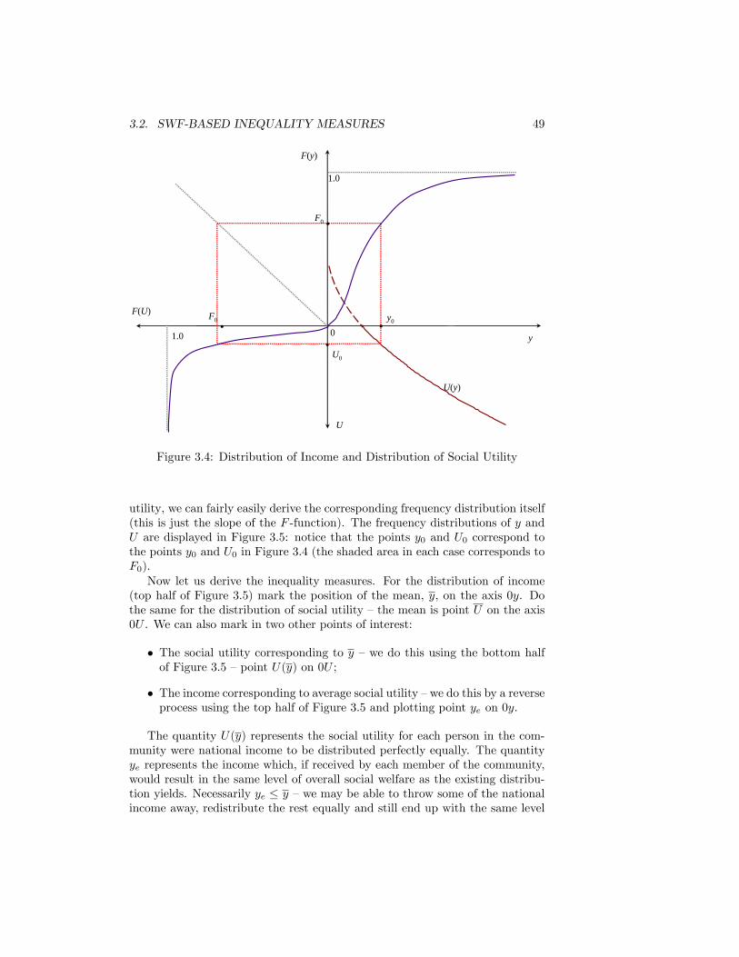
3.2. SWF-BASED INEQUALITY MEASURES 49
y
U
F(y)
F(U)
1.0
1.0 0
F0
U(y)
F0 y0
U0
●
●
●
●
Figure 3.4: Distribution of Income and Distribution of Social Utility
utility, we can fairly easily derive the corresponding frequency distribution itself(this is just the slope of the F -function). The frequency distributions of y andU are displayed in Figure 3.5: notice that the points y0 and U0 correspond tothe points y0 and U0 in Figure 3.4 (the shaded area in each case corresponds toF0).Now let us derive the inequality measures. For the distribution of income
(top half of Figure 3.5) mark the position of the mean, y, on the axis 0y. Dothe same for the distribution of social utility �the mean is point U on the axis0U . We can also mark in two other points of interest:
� The social utility corresponding to y �we do this using the bottom halfof Figure 3.5 �point U(y) on 0U ;
� The income corresponding to average social utility �we do this by a reverseprocess using the top half of Figure 3.5 and plotting point ye on 0y.
The quantity U(y) represents the social utility for each person in the com-munity were national income to be distributed perfectly equally. The quantityye represents the income which, if received by each member of the community,would result in the same level of overall social welfare as the existing distribu-tion yields. Necessarily ye � y �we may be able to throw some of the nationalincome away, redistribute the rest equally and still end up with the same level
50 CHAPTER 3. ANALYSING INEQUALITY
Figure 3.5: The Atkinson and Dalton Indices
of social welfare. Notice that we have drawn the diagram for a particular isoe-lastic utility function in the bottom right-hand quadrant of Figure 3.4; if " werechanged, then so would the frequency distribution in the bottom half of Figure3.5, and of course the positions of y and ye.
Thus we can de�ne a di¤erent inequality measure for each value of ", theinequality aversion parameter. An intuitively appealing way of measuring in-equality seems to be to consider how far actual average social utility falls shortof potential average social utility (if all income were distributed equally). So wede�ne Dalton�s Inequality Index (for inequality aversion ") as:
D" = 1�1n
Pni=1
�y1�"i � 1
�y1�" � 1
;
3.2. SWF-BASED INEQUALITY MEASURES 51
which in terms of the diagram means
D" = 1�U
U(y):
We may note that this is zero for perfectly equally distributed incomes (inwhich case we would have exactly U = U(y). Atkinson (1970) criticises the useof D" on the grounds that it is sensitive to the level from which social utilityis measured �if you add a non-zero constant to all the Us, D" changes. Nowthis does not change the ordering properties of D" over di¤erent distributionswith the same mean, but the inequality measures obtained by adding di¤erentarbitrary constants to U will not be cardinally equivalent. So Atkinson suggests,in e¤ect, that we perform our comparisons back on the 0y axis, not the 0U axis,and compare the �equally distributed equivalent�income, ye, with the mean y.To do this, we write U�1 for the inverse of the function U (so that U�1 (A)gives the income that would yield social-utility level A). Then we can de�neAtkinson�s Inequality Index (for inequality aversion ") as just
A" = 1�U�1
�U�
y;
where, as before, U is just average social utility 1n
Pni=1 U(yi). Using the explicit
formula (3.3) for the function U we get
A" = 1�"1
n
nXi=1
�yiy
�1�"# 11�"
:
In terms of the diagram this is:
A" = 1�yey:
Once again, as for the index D", we �nd a di¤erent value of A" for di¤erentvalues of our aversion to inequality.From the de�nitions we can check that the following relationship holds for
all distributions and all values of "
1�D" =U(y [1�A"])
U(y);
which means that@D"
@A"= y
U 0(y [1�A"])U 0(y)
> 0:
Clearly, in the light of this property, the choice between the indices D" andA"as de�ned above, is only of vital importance with respect to their cardinalproperties (�is the reduction in inequality by taxation greater in year A than inyear B?�); they are obviously ordinally equivalent in that they produce the same
52 CHAPTER 3. ANALYSING INEQUALITY
ranking of di¤erent distributions with the same mean.4 Of much greater signif-icance is the choice of the value of ", especially where Lorenz curves intersect,as in Figure 2.11. This re�ects our relative sensitivity to redistribution fromthe rich to the not-so-rich vis à vis redistribution from the not-so-poor to thepoor. The higher the value of "used the more sensitive is the index to changes indistribution at the bottom end of the parade �we will come to speci�c examplesof this later in the chapter.The advantage of the SWF approach is evident. Once agreed on the form
of the social-welfare function (for example along the lines of assumptions that Ihave listed above) it enables the analyst of inequality to say, in e¤ect �you tellme how strong society�s aversion to inequality is, and I will tell you the valueof the inequality statistic,�rather than simply incorporating an arbitrary socialweighting in an inequality index that just happens to be convenient.
3.3 Inequality and information theory
Probability distributions sometimes provide useful analogies for income distri-butions. In this section we shall see that usable and quite reasonable inequalitymeasures may be built up from an analogy with information theory.In information theory, one is concerned with the problem of �valuing� the
information that a certain event out of a large number of possibilities has oc-curred. Let us suppose that there are events numbered 1,2,3,..., to which weattach probabilities p1; p2; p3,... Each pi is not less than zero (which representstotal impossibility of event�s occurrence) and not greater than one (which rep-resents absolute certainty of the event�s occurrence). Suppose we are told thatevent #1 has occurred . We want to assign a number h(p1) to the value of thisinformation: how do we do this?If event #1 was considered to be quite likely anyway (p1 near to 1), then
this information is not �ercely exciting, and so we want h(p1) to be rather low;but if event #1 was a near impossibility, then this information is amazing andvaluable �it gets a high h(p1). So the implied value h(p1) should decrease as p1increases. A further characteristic which it seems correct that h(:) should have(in the context of probability analysis) is as follows. If event 1 and event 2 arestatistically independent (so that the probability that event 1 occurs does notdepend on whether or not event 2 occurs, and vice versa), then the probabilitythat both event 1 and event 2 occur together is p1p2. So, if we want to be ableto add up the information values of messages concerning independent events,
4 Instead of lying between zero and unity D" lies between 0 and 1. In order to transformthis into an inequality measure that is comparable with others we have used, it would benecessary to look at values of D"=[D" � 1]: One might be tempted to suggested that D" isthus a suitable choice as A". However, even apart from the fact that D" depends on thecardinalisation of utility there is another unsatisfactory feature of the relationship betweenD" and ". For Atkinson�s measure, A"; the higher is the value of ", the greater the value ofthe inequality measure for any given distribution; but this does not hold for D".
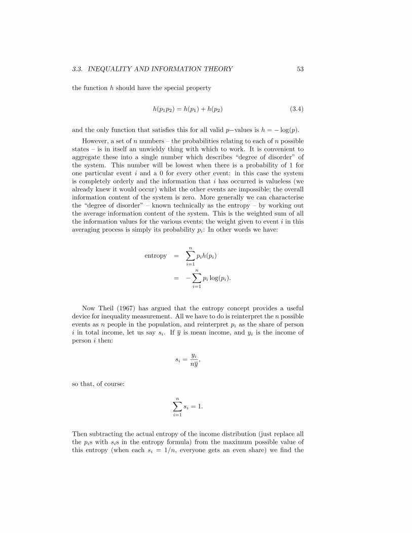
3.3. INEQUALITY AND INFORMATION THEORY 53
the function h should have the special property
h(p1p2) = h(p1) + h(p2) (3.4)
and the only function that satis�es this for all valid p�values is h = � log(p).However, a set of n numbers �the probabilities relating to each of n possible
states � is in itself an unwieldy thing with which to work. It is convenient toaggregate these into a single number which describes �degree of disorder� ofthe system. This number will be lowest when there is a probability of 1 forone particular event i and a 0 for every other event: in this case the systemis completely orderly and the information that i has occurred is valueless (wealready knew it would occur) whilst the other events are impossible; the overallinformation content of the system is zero. More generally we can characterisethe �degree of disorder��known technically as the entropy �by working outthe average information content of the system. This is the weighted sum of allthe information values for the various events; the weight given to event i in thisaveraging process is simply its probability pi: In other words we have:
entropy =nXi=1
pih(pi)
= �nXi=1
pi log(pi):
Now Theil (1967) has argued that the entropy concept provides a usefuldevice for inequality measurement. All we have to do is reinterpret the n possibleevents as n people in the population, and reinterpret pi as the share of personi in total income, let us say si. If y is mean income, and yi is the income ofperson i then:
si =yiny;
so that, of course:
nXi=1
si = 1:
Then subtracting the actual entropy of the income distribution (just replace allthe pis with sis in the entropy formula) from the maximum possible value ofthis entropy (when each si = 1=n, everyone gets an even share) we �nd the
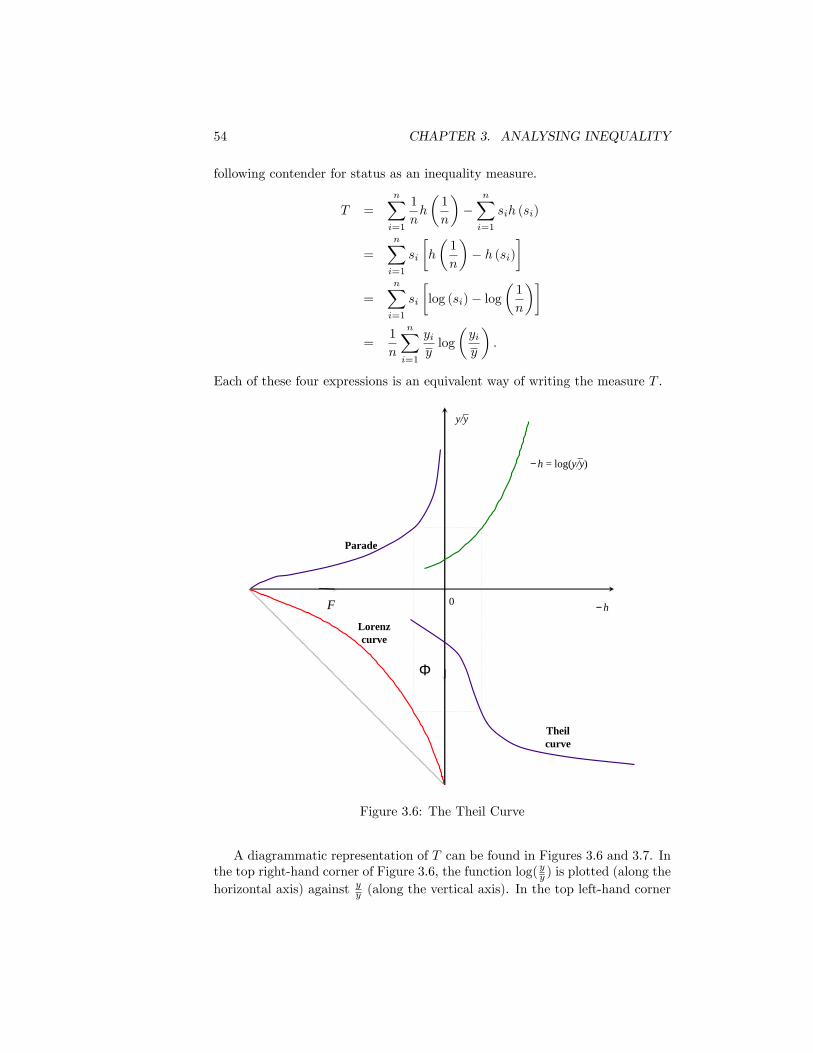
54 CHAPTER 3. ANALYSING INEQUALITY
following contender for status as an inequality measure.
T =nXi=1
1
nh
�1
n
��
nXi=1
sih (si)
=nXi=1
si
�h
�1
n
�� h (si)
�
=nXi=1
si
�log (si)� log
�1
n
��
=1
n
nXi=1
yiylog
�yiy
�:
Each of these four expressions is an equivalent way of writing the measure T .
− h
y/y_
Φ
− h = log(y/y)_
Parade
Lorenzcurve
Theilcurve
F 0
Figure 3.6: The Theil Curve
A diagrammatic representation of T can be found in Figures 3.6 and 3.7. Inthe top right-hand corner of Figure 3.6, the function log(yy ) is plotted (along thehorizontal axis) against y
y (along the vertical axis). In the top left-hand corner
3.3. INEQUALITY AND INFORMATION THEORY 55
we have the Parade, slightly modi�ed from Figure 2.1, whilst in the bottomleft-hand corner we have the Lorenz curve (upside down). We can use thesethree curves to derive the Theil curve in the bottom right hand corner of Figure3.6. The method is as follows.
� Pick a particular value of F .
� Use the Parade diagram (top left) to �nd the corresponding value of y=y�in other words the appropriate quantile divided by the mean.
� Also use the Lorenz curve (bottom left) to �nd the corresponding �-valuefor this same F -value �in other words �nd the income share of the groupin population that has an income less than or equal to y.
� Read o¤ the ��h�value corresponding to yy using the log function shown
top right.
� You have now �xed a particular point in the bottom right-hand part ofthe �gure as shown by dotted rectangle.
� By repeating this for every other F -value, trace out a curve �the Theilcurve �in the bottom right-hand corner.
If you are not yet convinced, you may care to try plotting another set of fourpoints as an exercise. This Theil curve charts the �information function�againstincome shares. Unfortunately the entire curve cannot be shown in Figure 3.6since it crosses the 0� axis ; to remedy this I have drawn a fuller picture ofthe curve in Figure 3.7, (which is drawn the logical way up, with 0� along thehorizontal axis). The measure T is then simply the area trapped between thiscurve and the 0� axis �shown as a shaded area.However, this merely tells us about the mechanics of Theil�s measure; we
need to look more closely at its implications for the way we look at inequality.To do this, examine what happens to T if the share of a poor person (1) isincreased at the expense of a rich person (2). So let the share of person 1increase from s1 to a fractionally larger amount s1 + 4s and the share of 2decrease to s2 � 4s. Then, remembering that h(s) = � log(s), we �nd (bydi¤erentiation) that the resulting change in T is:
�T = �s [h (s2)� h (s1)]
= ��s log�s2s1
�:
As we would expect, the proposed transfer 4s results in a negative 4T , so thatthe inequality index decreases. But we can say a little more than that. Wesee that the size of the reduction in T depends only on the ratio of s2 to s1.So for any two people with income shares in the same ratio, the transfer s (asabove) would lead to the same reduction in inequality T . Thus, for example, asmall transfer from a person with an income share of 2 millionths, to a person
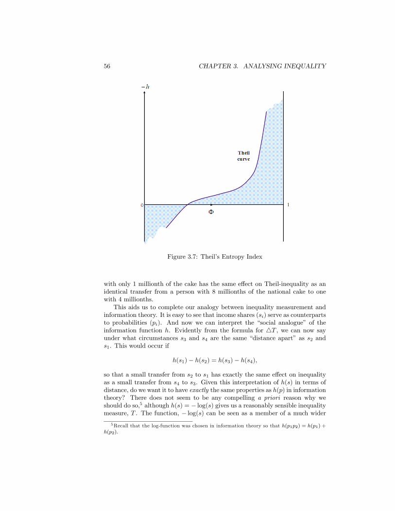
56 CHAPTER 3. ANALYSING INEQUALITY
Figure 3.7: Theil�s Entropy Index
with only 1 millionth of the cake has the same e¤ect on Theil-inequality as anidentical transfer from a person with 8 millionths of the national cake to onewith 4 millionths.This aids us to complete our analogy between inequality measurement and
information theory. It is easy to see that income shares (si) serve as counterpartsto probabilities (pi). And now we can interpret the �social analogue� of theinformation function h. Evidently from the formula for 4T , we can now sayunder what circumstances s3 and s4 are the same �distance apart� as s2 ands1. This would occur if
h(s1)� h(s2) = h(s3)� h(s4);
so that a small transfer from s2 to s1 has exactly the same e¤ect on inequalityas a small transfer from s4 to s3. Given this interpretation of h(s) in terms ofdistance, do we want it to have exactly the same properties as h(p) in informationtheory? There does not seem to be any compelling a priori reason why weshould do so,5 although h(s) = � log(s) gives us a reasonably sensible inequalitymeasure, T . The function, � log(s) can be seen as a member of a much wider
5Recall that the log-function was chosen in information theory so that h(p1p2) = h(p1) +h(p2):
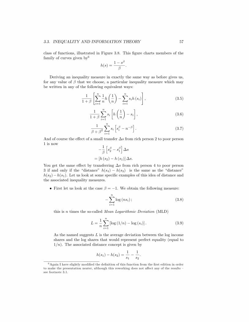
3.3. INEQUALITY AND INFORMATION THEORY 57
class of functions, illustrated in Figure 3.8. This �gure charts members of thefamily of curves given by6
h(s) =1� s��
:
Deriving an inequality measure in exactly the same way as before gives us,for any value of � that we choose, a particular inequality measure which maybe written in any of the following equivalent ways:
1
1 + �
"nXi=1
1
nh
�1
n
��
nXi=1
sih (si)
#; (3.5)
1
1 + �
nXi=1
si
�h
�1
n
�� si
�; (3.6)
1
� + �2
nXi=1
si
hs�i � n��
i: (3.7)
And of course the e¤ect of a small transfer �s from rich person 2 to poor person1 is now
� 1�
hs�2 � s
�1
i�s
= [h (s2)� h (s1)]�s:You get the same e¤ect by transferring �s from rich person 4 to poor person3 if and only if the �distance� h(s4) � h(s3) is the same as the �distance�h(s2)�h(s1). Let us look at some speci�c examples of this idea of distance andthe associated inequality measures.
� First let us look at the case � = �1. We obtain the following measure:
�nXi=1
log (nsi) ; (3.8)
this is n times the so-called Mean Logarithmic Deviation (MLD)
L =1
n
nXi=1
[log (1=n)� log (si)] : (3.9)
As the named suggests L is the average deviation between the log incomeshares and the log shares that would represent perfect equality (equal to1=n). The associated distance concept is given by
h(s1)� h(s2) =1
s1� 1
s2:
6Again I have slightly modi�ed the de�nition of this function from the �rst edition in orderto make the presentation neater, although this reworking does not a¤ect any of the results �see footnote 3.1.
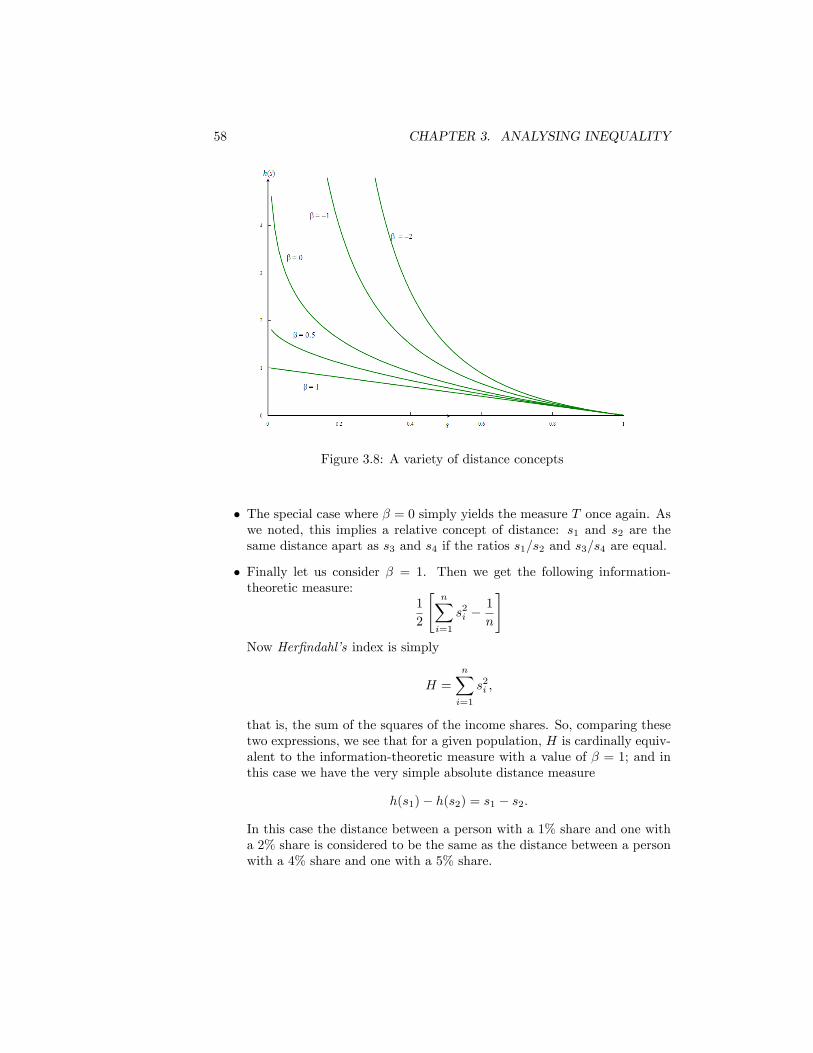
58 CHAPTER 3. ANALYSING INEQUALITY
Figure 3.8: A variety of distance concepts
� The special case where � = 0 simply yields the measure T once again. Aswe noted, this implies a relative concept of distance: s1 and s2 are thesame distance apart as s3 and s4 if the ratios s1=s2 and s3=s4 are equal.
� Finally let us consider � = 1. Then we get the following information-theoretic measure:
1
2
"nXi=1
s2i �1
n
#Now Her�ndahl�s index is simply
H =
nXi=1
s2i ;
that is, the sum of the squares of the income shares. So, comparing thesetwo expressions, we see that for a given population, H is cardinally equiv-alent to the information-theoretic measure with a value of � = 1; and inthis case we have the very simple absolute distance measure
h(s1)� h(s2) = s1 � s2:
In this case the distance between a person with a 1% share and one witha 2% share is considered to be the same as the distance between a personwith a 4% share and one with a 5% share.

3.3. INEQUALITY AND INFORMATION THEORY 59
income shareperson P £ 2 000 0.2%
... ... ...person Q £ 10 000 1.0%
... ... ...person R £ 50 000 5.0%
... ... ...all: £ 1 000 000 100%
distance distance� h(si)� h(sj) (P,Q) (Q,R)�1 1
si� 1
sj400 80
0 log(sjsi) log(5) log(5)
1 sj � si 0:008 0:04
Table 3.2: Is P further from Q than Q is from R?
Thus, by choosing an appropriate �distance function�, we determine a par-ticular �information theoretic�inequality measure. In principle we can do thisfor any value of �. Pick a particular curve in Figure 3.8: the �distance�betweenany two income shares on the horizontal axis is given by the linear distance be-tween their two corresponding points on the vertical axis. The �-curve of ourchoice (suitably rotated) can then be plugged into the top left-hand quadrant ofFigure 3.6, and we thus derive a new curve to replace the original in the bottomright-hand quadrant, and obtain the modi�ed information-theoretic inequalitymeasure. Each distance concept is going to give di¤erent weight on the gapsbetween income shares in di¤erent parts of the income distribution. To illus-trate this, have a look at the example in Table 3.2: the top part of this givesthe income for three (out of many) individuals, poor P, rich R and quite-well-o¤Q, and their respective shares in total income (assumed to be £ 1 000 000); thebottom part gives the implied distance from P to Q and the implied distancefrom Q to R for three of the special values of � that we have discussed in detail.We can see that for � = �1 the (P,Q)-gap is ranked as greater than the (Q,R)-gap; for � = 1 the reverse is true; and for � = 0, the two gaps are regarded asequivalent.Notice the formal similarity between choosing one of the curves in Figure
3.8 and choosing a social utility function or welfare index in Figure 3.1. Ifwe write � = �" , the analogy appears to be almost complete: the choice of�distance function� seems to be determined simply by our relative inequalityaversion. Yet the approach of this section leads to inequality measures thatare somewhat di¤erent from those found previously. The principal di¤erenceconcerns the inequality measures when � � 0. As we have seen the modi�edinformation-theoretic measure is de�ned for such values. However, A" and D"
become trivial when " is zero (since A0 and D0 are zero whatever the income
60 CHAPTER 3. ANALYSING INEQUALITY
distribution); and usually neither A" nor D" is de�ned for " < 0 (correspondingto � > 0). Furthermore, even for positive values of " �where the appropriatemodi�ed information-theoretic measure ranks any set of income distributions inthe same order as A" and D" �it is evident that the Atkinson index, the Daltonindex and the information-theoretic measure will not be cardinally equivalent.Which forms of inequality measure should we choose then? The remainder ofthis chapter will deal more fully with this important issue.
3.4 Building an inequality measure
What we shall now do is consider more formally the criteria we want satis�ed byinequality measures. You may be demanding why this has not been done before.The reason is that I have been anxious to trace the origins of inequality measuresalready in use and to examine the assumptions required at these origins.
� Weak Principle of Transfers� Income Scale Independence� Principle of Population� Decomposability
� Strong Principle of Transfers
FIVE PROPERTIES OF INEQUALITY MEASURES
However, now that we have looked at ad hoc measures, and seen how theSWF and information theory approaches work, we can collect our thoughts onthe properties of these measures. The importance of this exercise lies not onlyin the drawing up of a shortlist of inequality measures by eliminating those thatare �unsuitable.� It also helps to put personal preference in perspective whenchoosing among those cited in the shortlist. Furthermore it provides the basis forthe third approach of this chapter: building a particular class of mathematicalfunctions for use as inequality measures from the elementary properties that wemight think that inequality measures ought to have. It is in e¤ect a structuralapproach to inequality measurement.This is a trickier task, but rewarding, nonetheless; to assist us there is a
check-list of the proposed elementary criteria in the accompanying box. Let uslook more closely at the �rst four of these: the �fth criterion will be discusseda bit later.
Weak Principle of Transfers
In Chapter 2 we were interested to note whether each of the various inequalitymeasures discussed there had the property that a hypothetical transfer of incomefrom a rich person to a poor person reduces measured inequality. This property
3.4. BUILDING AN INEQUALITY MEASURE 61
may now be stated more precisely. We shall say that an inequality measuresatis�es the weak principle of transfers if the following is always true. Considerany two individuals, one with income y, the other, a richer person, with incomey + � where � is positive. Then transfer a positive amount of income 4y fromthe richer to the poorer person, where 4y is less than 2�. Inequality shouldthen de�nitely decrease. If this property is true for some inequality measure,no matter what values of y and y + � we use, then we may use the followingtheorem.
Theorem 4 Suppose the distribution of income in social state A could be achievedby a simple redistribution of income in social state B (so that total income isthe same in each case) and the Lorenz curve for A lies wholly inside that of B.Then, as long as an inequality measure satis�es the weak principle of transfers,that inequality measure will always indicate a strictly lower level of inequalityfor state A than for state B.
This result is not exactly surprising, if we recall the interpretation of theLorenz curve in Chapter 2: if you check the example given in Figure 2.10 onpage 33 you will see that we could have got to state A from state B by a seriesof richer-to-poorer transfers of the type mentioned above. However, Theorem4 emphasises the importance of this principle for choosing between inequalitymeasures. As we have seen V , c, G, L, T , H, A", D" (" > 0) and the modi�edinformation-theory indices all pass this test; � and �1 fail the test in the caseof high incomes �it is possible for these to rank B as superior to A. The othermeasures, R, M , the equal shares coe¢ cient, etc., just fail the test �for thesemeasures it would be possible for state A�s Lorenz curve to lie partly �inside�and to lie nowhere �outside� that of state B, and yet exhibit no reduction inmeasured inequality. In other words, we have achieved a situation where therehas been some richer-to-poorer redistribution somewhere in the population, butapparently no change in inequality occurs.7
I have quali�ed the de�nition given above as the weak principle of transfers,because all that it requires is that given the speci�ed transfer, inequality shoulddecrease. But it says nothing about how much it should decrease. This point isconsidered further when we get to the �nal item on the list of properties.
Income Scale Independence
This means that the measured inequality of the slices of the cake should notdepend on the size of the cake. If everyone�s income changes by the sameproportion then it can be argued that there has been no essential alteration inthe income distribution, and thus that the value of the inequality measure shouldremain the same. This property is possessed by all the inequality measures wehave examined, with the exception of the variance V , and Dalton�s inequality
7However, this type of response to a transfer might well be appropriate for poverty measuressince these tools are designed for rather di¤erent purposes.
62 CHAPTER 3. ANALYSING INEQUALITY
indices.8 This is immediately evident in the case of those measures de�ned withrespect to income shares si, since a proportional income change in all incomesleaves the shares unchanged.
Principle of Population
This requires that the inequality of the cake distribution should not depend onthe number of cake-receivers. If we measure inequality in a particular economywith n people in it and then merge the economy with another identical one, weget a combined economy with a population of 2n, and with the same proportionof the population receiving any given income. If measured inequality is the samefor any such replication of the economy, then the inequality measure satis�esthe principle of population.However, it is not self-evident that this property is desirable. Consider a
two-person world where one person has all the income, and the other has none.Then replicate the economy as just explained, so that one now has a four-personworld with two destitute people and two sharing income equally. It seems tome debatable whether these two worlds are �equally unequal.� In fact nearlyall the inequality measures we have considered would indicate this, since theysatisfy the principle of population. The notable exceptions are the modi�edinformation-theoretic indices: if � = 0 (the original Theil index) the populationprinciple is satis�ed, but otherwise as the population is increased the measurewill either increase (the case where � < 0) or decrease (the case where � > 0,including Her�ndahl�s index of course). However, as we shall see in a moment,it is possible to adapt this class of measures slightly so that the populationprinciple is always satis�ed.
Decomposability
This property implies that there should be a coherent relationship between in-equality in the whole of society and inequality in its constituent parts. Thebasic idea is that we would like to be able to write down a formula giving totalinequality as a function of inequality within the constituent subgroups, and in-equality between the subgroups. More ambitiously we might hope to be able toexpress the within-group inequality as something like an average of the inequal-ity in each individual sub-group. However, in order to do either of these thingswith an inequality measure it must have an elementary consistency property:that inequality rankings of alternative distributions in the population as a wholeshould match the inequality rankings of the corresponding distributions withinany the subgroups of which the population is composed.This can be illustrated using a pair of examples, using arti�cial data specially
constructed to demonstrate what might appear as a curious phenomenon. In the�rst we consider an economy of six persons that is divided into two equal-sizedparts, East and West. As is illustrated in Table 3.3, the East is much poorer
8Whether a Dalton index satis�es scale independence or not will depend on the particularcardinalisation of the function U that is used.
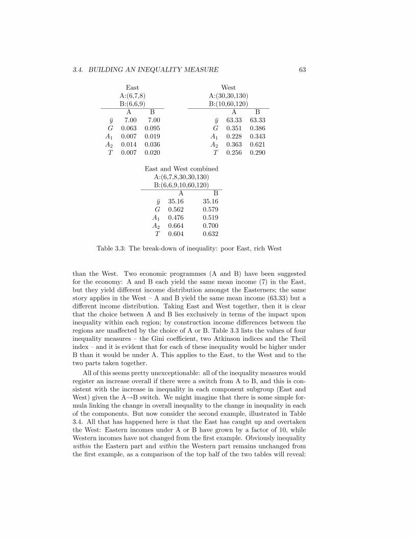
3.4. BUILDING AN INEQUALITY MEASURE 63
East WestA:(6,7,8) A:(30,30,130)B:(6,6,9) B:(10,60,120)A B A B
�y 7.00 7.00 �y 63.33 63.33G 0.063 0.095 G 0.351 0.386A1 0.007 0.019 A1 0.228 0.343A2 0.014 0.036 A2 0.363 0.621T 0.007 0.020 T 0.256 0.290
East and West combinedA:(6,7,8,30,30,130)B:(6,6,9,10,60,120)
A B�y 35.16 35.16G 0.562 0.579A1 0.476 0.519A2 0.664 0.700T 0.604 0.632
Table 3.3: The break-down of inequality: poor East, rich West
than the West. Two economic programmes (A and B) have been suggestedfor the economy: A and B each yield the same mean income (7) in the East,but they yield di¤erent income distribution amongst the Easterners; the samestory applies in the West �A and B yield the same mean income (63.33) but adi¤erent income distribution. Taking East and West together, then it is clearthat the choice between A and B lies exclusively in terms of the impact uponinequality within each region; by construction income di¤erences between theregions are una¤ected by the choice of A or B. Table 3.3 lists the values of fourinequality measures �the Gini coe¢ cient, two Atkinson indices and the Theilindex �and it is evident that for each of these inequality would be higher underB than it would be under A. This applies to the East, to the West and to thetwo parts taken together.
All of this seems pretty unexceptionable: all of the inequality measures wouldregister an increase overall if there were a switch from A to B, and this is con-sistent with the increase in inequality in each component subgroup (East andWest) given the A!B switch. We might imagine that there is some simple for-mula linking the change in overall inequality to the change in inequality in eachof the components. But now consider the second example, illustrated in Table3.4. All that has happened here is that the East has caught up and overtakenthe West: Eastern incomes under A or B have grown by a factor of 10, whileWestern incomes have not changed from the �rst example. Obviously inequalitywithin the Eastern part and within the Western part remains unchanged fromthe �rst example, as a comparison of the top half of the two tables will reveal:
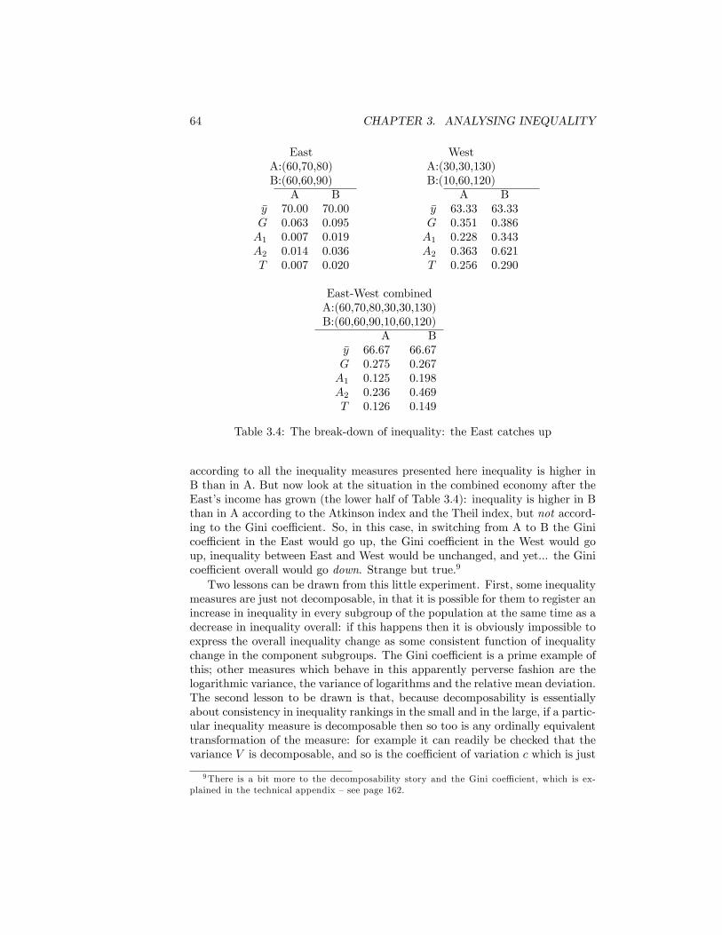
64 CHAPTER 3. ANALYSING INEQUALITY
East WestA:(60,70,80) A:(30,30,130)B:(60,60,90) B:(10,60,120)
A B A B�y 70.00 70.00 �y 63.33 63.33G 0.063 0.095 G 0.351 0.386A1 0.007 0.019 A1 0.228 0.343A2 0.014 0.036 A2 0.363 0.621T 0.007 0.020 T 0.256 0.290
East-West combinedA:(60,70,80,30,30,130)B:(60,60,90,10,60,120)
A B�y 66.67 66.67G 0.275 0.267A1 0.125 0.198A2 0.236 0.469T 0.126 0.149
Table 3.4: The break-down of inequality: the East catches up
according to all the inequality measures presented here inequality is higher inB than in A. But now look at the situation in the combined economy after theEast�s income has grown (the lower half of Table 3.4): inequality is higher in Bthan in A according to the Atkinson index and the Theil index, but not accord-ing to the Gini coe¢ cient. So, in this case, in switching from A to B the Ginicoe¢ cient in the East would go up, the Gini coe¢ cient in the West would goup, inequality between East and West would be unchanged, and yet... the Ginicoe¢ cient overall would go down. Strange but true.9
Two lessons can be drawn from this little experiment. First, some inequalitymeasures are just not decomposable, in that it is possible for them to register anincrease in inequality in every subgroup of the population at the same time as adecrease in inequality overall: if this happens then it is obviously impossible toexpress the overall inequality change as some consistent function of inequalitychange in the component subgroups. The Gini coe¢ cient is a prime example ofthis; other measures which behave in this apparently perverse fashion are thelogarithmic variance, the variance of logarithms and the relative mean deviation.The second lesson to be drawn is that, because decomposability is essentiallyabout consistency in inequality rankings in the small and in the large, if a partic-ular inequality measure is decomposable then so too is any ordinally equivalenttransformation of the measure: for example it can readily be checked that thevariance V is decomposable, and so is the coe¢ cient of variation c which is just
9There is a bit more to the decomposability story and the Gini coe¢ cient, which is ex-plained in the technical appendix �see page 162.
3.5. CHOOSING AN INEQUALITY MEASURE 65
the square root of V .There is a powerful result that clari�es which inequality measures will satisfy
decomposability along with the other properties that we have discussed so far:
Theorem 5 Any inequality measure that simultaneously satis�es the propertiesof the weak principle of transfers, decomposability, scale independence and thepopulation principle must be expressible either in the form
E� =1
�2 � �
"1
n
nXi=1
�yi�y
��� 1#;
or as J(E�), some ordinally-equivalent transformation of E�, where � is a realparameter that may be given any value, positive, zero or negative.
I have used the symbol �E� to denote this family of measures, since theyhave become known in the literature as the generalised entropy measures. Aquick comparison of this formula with that of the modi�ed information-theoreticmeasures (de�ned on page 57) shows that the two are very closely related: infact the generalised entropy measures are just the modi�ed-information theoreticfamily again, now normalised so that they satisfy the population principle, andwith the parameter � set equal to � � 1.10 In view of this �family connection�it is clear that the generalised entropy measures have other connections too:inspection of the generalised entropy formula reveals that the case � = 2 yieldsan index that is cardinally equivalent to the Her�ndahl index H (and henceordinally equivalent to V and c); putting � = 1 � " in the formula we cansee that � for values of � < 1 �the measures are ordinally equivalent to thewelfare-theoretic indices A" and D" for distributions with a given mean.As with our discussion of welfare-based and information-theory based mea-
sures we have now have a collection or family of inequality measures that in-corporates a set of principles for ranking income distributions. And, as we havejust seen, there are close connections between all the indices derived from threeapproaches. Let us see if we can narrow things down a bit further.
3.5 Choosing an inequality measure
Now that we have seen three approaches to a coherent and comprehensive analy-sis of inequality, how should we go about selecting an appropriate inequalitymeasurement tool? For a start let us clarify the nature of the choice that we areto make. We need to make the important distinction between choosing a familyof inequality measures and choosing a particular member from the family. Thissort of distinction would apply to the selection of mathematical functions inother contexts. For example if we were decorating a piece of paper and wanted
10 In the �rst edition (1977) the modi�ed information-theoretic measure was denoted I� andextensively discussed. Since that time the literature has more frequently used the normali-sation of the Generalised entropy family given here as E� . Formally one has E1 = I0 = T; if� = 1 (� = 0), and E� = I��1n��1 for other values of �:
66 CHAPTER 3. ANALYSING INEQUALITY
to decide on a particular curve or shape to use in the pattern, we might consider�rst the broader choice between families of curves or shapes �squares, circles,triangles, ellipses,... �and then having decided upon ellipses for the design per-haps we would want to be more speci�c and pick a particular size and shape ofellipse. Some of the broad principles that we have considered under �buildingan inequality measure�are rather like the questions at the level of the �squares,circles or ellipses?�stage of designing the decorative pattern. Let us see whatguidance we now have in choosing a family of inequality measures.The �rst four of the basic properties of inequality measures that we listed ear-
lier �the weak transfer principle, scale independence, the population principleand decomposability �would probably command wide although not universalsupport. As we have seen they de�ne an extended family of measures: the gen-eralised entropy family and all the measures that are ordinally equivalent to it.It may be worth trying to narrow this selection of measures a bit further, andto do this we should discuss the �fth on the list of the basic principles.
Strong Principle of Transfers
Let us recall the concept of �distance�between people�s income shares, intro-duced on page 56 to strengthen the principle of transfers. Consider a distancemeasure given by
d = h(s1)� h(s2);
where s2 is greater than s1, and h(s) is one of the curves in Figure 3.8. Thenconsider a transfer from rich person 2 to poor person 1. We say that the inequal-ity measure satis�es the principle of transfers in the strong sense if the amountof the reduction in inequality depends only on d, the distance, no matter whichtwo individuals we choose.For the kind of h-function illustrated in Figure 3.8, the inequality measures
that satisfy this strong principle of transfers belong to the family describedby formulas for the modi�ed information-theoretic family (of which the Theilindex and the Her�ndahl index are special cases) or the generalised entropyfamily which, as we have just seen is virtually equivalent. Each value of �� equivalently each value of � � de�nes a di¤erent concept of distance, andthus a di¤erent associated inequality measure satisfying the strong principle oftransfers.In e¤ect we have found an important corollary to Theorem 5. Adding the
strong principle of transfers to the other criteria means that Theorem 5 can bestrengthened a bit: if all �ve properties listed above are to be satis�ed then theonly measures which will do the job are the generalised entropy indices E�.Why should we want to strengthen the principle of transfers in this way?
One obvious reason is that merely requiring that a measure satisfy the weakprinciple gives us so much latitude that we cannot even �nd a method of rankingall possible income distributions in an unambiguous order. This is because, asTheorem 4 shows, the weak principle amounts to a requirement that the measureshould rank income distributions in the same fashion as the associated Lorenz
3.5. CHOOSING AN INEQUALITY MEASURE 67
curves �no more, no less. Now the strong principle of transfers by itself doesnot give this guidance, but it points the way to an intuitively appealing method.Several writers have noted that an inequality measure incorporates some sort ofaverage of income di¤erences. The �distance�concept, d, allows one to formalisethis. For, given a particular d, one may derive a particular inequality measureby using the strong principle as a fundamental axiom.11 This measure takesthe form of the average distance between each person�s actual income and theincome he would receive in a perfectly equal society, and is closely related toE�.12 The advantage of this is that instead of postulating the existence of asocial-welfare function, discussing its desired properties, and then deriving themeasure, one may discuss the basic idea of distance between income shares andthen derive the inequality measure directly.Most of the ad hoc inequality measures do not satisfy the strong principle
of transfers as they stand, although some are ordinally equivalent to measuressatisfying this axiom. In such cases, the size of a change in inequality due toan income transfer depends not only on the distance between the shares of thepersons concerned, but on the measured value of overall inequality as well. Itis interesting to note the distance concept implied by these measures. Implicitin the use of the variance and the coe¢ cient of variation (which are ordinallyequivalent to H) is the notion that distance equals the absolute di¤erence be-tween income shares. The relative mean deviation implies a very odd notionof distance �zero if both persons are on the same side of the mean, and oneif they are on opposite sides. This property can be deduced from the e¤ect ofthe particular redistribution illustrated in Figure 2.6. The measures �; �1and Gare not even ordinally equivalent to a measure satisfying the strong principle.In the case of � and �1 this is because they do not satisfy the weak principleeither; the reason for G�s failure is more subtle. Here the size of the changein inequality arising from a redistribution between two people depends on theirrelative position in the Parade, not on the absolute size of their incomes or theirincome shares. Hence a redistribution from the 4th to the 5th person (arrangedin parade order) has the same e¤ect as a transfer from the 1 000 004th to the 1000 005th, whatever their respective incomes. So distance cannot be de�ned interms of the individual income shares alone.A further reason for recommending the strong principle lies in the cardinal
properties of inequality measures. In much of the literature attention is focusedon ordinal properties, and rightly so. However, sometimes this has meant thatbecause any transformation of an inequality measure leaves its ordering proper-ties unchanged, cardinal characteristics have been neglected or rather arbitrarilyspeci�ed. For example, it is sometimes recommended that the inequality mea-sure should be normalised so that it always lies between zero and one. To usethis as a recommendation for a particular ordinally equivalent variant of theinequality measure is dubious for three reasons.
11For the other axioms required see Cowell and Kuga (1981) and the discussion on page 186which give an overview of the development of this literature.12This is clear from the second of the three ways in which the information-theoretic measure
was written down on page 57.
68 CHAPTER 3. ANALYSING INEQUALITY
1. It is not clear that a �nite maximum value of inequality, independent ofthe number in the population, is desirable.
2. There are many ways of transforming the measure such that it lies inthe zero-to-one range, each such transformation having di¤erent cardinalproperties.
3. And, in particular, where the untransformed measure has a �nite maxi-mum, the measure can easily be normalised without altering its cardinalproperties simply by dividing by that maximum value.13
However, because measures satisfying the strong principle of transfers canbe written down as the sum of a function of each income share, they haveattractive cardinal properties when one considers either the problem of decom-posing inequality by population subgroups (as in the East-West example dis-cussed above), or of quantifying changes in measured inequality. The familyE�, all members of which satisfy the strong principle, may be written in sucha way that changes in inequality overall can easily be related to (a) changesin inequality within given subgroups of the population, and (b) changes in theincome shares enjoyed by these subgroups, and hence the inequality betweenthe groups. The way to do this is explained in the Technical Appendix, fromwhich it is clear that a measure such as A", though formally ordinally equiv-alent to I� for many values of ", does not decompose nearly so easily. Thesecardinal properties are, of course, very important when considering empiricalapplications, as we do in Chapter 5.Now let us consider the second aspect of choice: the problem of selecting
from among a family of measures one particular index. As we have seen, many,though not all, of the inequality measures that are likely to be of interest will beordinally equivalent to the generalised entropy class: this applies for exampleto inequality measures that arise naturally from the SWF method (for examplewe know that all the measures A" are ordinally equivalent E�, for � = 1 � "where " > 0). Let us then take the generalised entropy family of measures14
�extended to include all the measures that are ordinally equivalent � as theselected family and examine the issues involved in picking one index from thefamily.If we are principally concerned with the ordering property of the measures,
then the key decision is the sensitivity of the inequality index to informationabout di¤erent parts of the distribution. We have already seen this issue in ourdiscussion on page 59 of whether the distance between Rich R and quite-well-o¤ Q was greater than the distance between Q and poor P. Di¤erent distanceconcepts will give di¤erent answers to this issue. The distance concept can beexpressed in terms of the value of the parameter � or, equivalently in terms of
13This assumes that the minimum value is zero; but the required normalisation is easywhatever the minimum value.14Although we could have constructed reasonable arguments for other sets of axioms that
would have picked out a di¤erent class of inequality measures � see the Technical Appendixfor a further discussion.
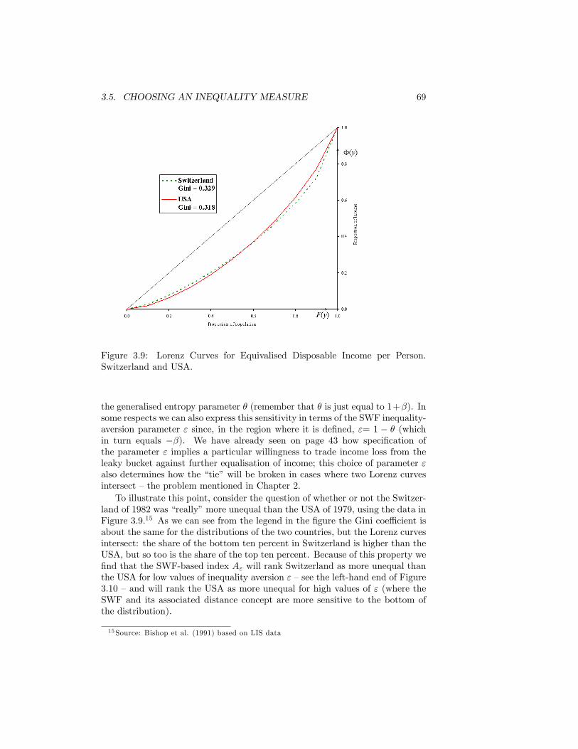
3.5. CHOOSING AN INEQUALITY MEASURE 69
Figure 3.9: Lorenz Curves for Equivalised Disposable Income per Person.Switzerland and USA.
the generalised entropy parameter � (remember that � is just equal to 1+�). Insome respects we can also express this sensitivity in terms of the SWF inequality-aversion parameter " since, in the region where it is de�ned, "= 1 � � (whichin turn equals ��). We have already seen on page 43 how speci�cation ofthe parameter " implies a particular willingness to trade income loss from theleaky bucket against further equalisation of income; this choice of parameter "also determines how the �tie�will be broken in cases where two Lorenz curvesintersect �the problem mentioned in Chapter 2.To illustrate this point, consider the question of whether or not the Switzer-
land of 1982 was �really�more unequal than the USA of 1979, using the data inFigure 3.9.15 As we can see from the legend in the �gure the Gini coe¢ cient isabout the same for the distributions of the two countries, but the Lorenz curvesintersect: the share of the bottom ten percent in Switzerland is higher than theUSA, but so too is the share of the top ten percent. Because of this property we�nd that the SWF-based index A" will rank Switzerland as more unequal thanthe USA for low values of inequality aversion " �see the left-hand end of Figure3.10 �and will rank the USA as more unequal for high values of " (where theSWF and its associated distance concept are more sensitive to the bottom ofthe distribution).
15Source: Bishop et al. (1991) based on LIS data
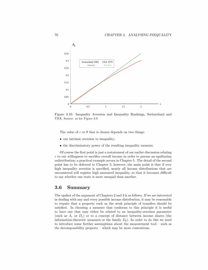
70 CHAPTER 3. ANALYSING INEQUALITY
0 0.5 1 1.5 20
0.05
0.1
0.15
0.2
0.25
0.3
0.35
Switzerland 1982 USA 1979
Aε
ε
Figure 3.10: Inequality Aversion and Inequality Rankings, Switzerland andUSA. Source: as for Figure 3.9
The value of " or � that is chosen depends on two things:
� our intrinsic aversion to inequality;
� the discriminatory power of the resulting inequality measure.
Of course the �rst point is just a restatement of our earlier discussion relating" to our willingness to sacri�ce overall income in order to pursue an egalitarianredistribution; a practical example occurs in Chapter 5. The detail of the secondpoint has to be deferred to Chapter 5; however, the main point is that if veryhigh inequality aversion is speci�ed, nearly all income distributions that areencountered will register high measured inequality, so that it becomes di¢ cultto say whether one state is more unequal than another.
3.6 Summary
The upshot of the argument of Chapters 2 and 3 is as follows. If we are interestedin dealing with any and every possible income distribution, it may be reasonableto require that a property such as the weak principle of transfers should besatis�ed. In choosing a measure that conforms to this principle it is usefulto have one that may either be related to an inequality-aversion parameter(such as A" or D") or to a concept of distance between income shares (theinformation-theoretic measures or the family E�). In order to do this we needto introduce some further assumptions about the measurement tool �such asthe decomposability property �which may be more contentious.
3.7. QUESTIONS 71
Even if these assumptions about building an inequality measure are accepted,this still leaves the question of various cardinal characteristics open. Invariancewith respect to proportional changes in all incomes or with respect to increasesin the population may be desirable under certain circumstances. Standardis-ation of the measure in a given range (such as 0 to 1) has only a super�cialattractiveness to recommend it: it may be well worth while sacri�cing this inorder to put the measure in a cardinal form more useful for analysing the com-position of, and changes in, inequality. The way these conclusions relate to themeasures we have mentioned is summarised in Table 3.5.However, these remarks apply to comparisons of all conceivable distributions.
You may wonder whether our task could be made easier if our attention wererestricted to those distributions that are, in some sense, more likely to arise.The next chapter attempts to deal with this issue.
3.7 Questions
1. Show that the inequality aversion parameter " is the elasticity of socialmarginal utility de�ned on page 41.
2.
(a) Use the UK 1984/5 data (see �le �ET income distribution� on thewebsite) to compute Atkinson�s inequality index with " = 2, makingthe same assumptions as in question 5 of Chapter 2.
(b) Recompute the index in part (a) after dropping the �rst income classfrom the data set. Why does measured inequality decrease?
(c) Rework the calculations in (b) for a variety of values of " so as toverify that measured inequality rises with inequality aversion for agiven data set.
3. Suppose that the assumption of constant relative inequality aversion (page41) were to be replaced by the assumption of constant absolute inequalityaversion, whereby the U -function may be written
U(yi) = �1
�e��yi :
(a) Sketch the U -function for di¤erent values of �.
(b) Write down the corresponding social-welfare function, and hence �ndan expression for the equally-distributed equivalent income;
(c) Explain what happens to social welfare as yi goes to zero. Is thesocial-welfare function de�ned for negative incomes?
4. Consider the following two distributions of income
A : (1; 4; 7; 10; 13);
B : (1; 5; 6; 10; 13):

72 CHAPTER 3. ANALYSING INEQUALITYIndex
Principle
ofDistance
Decom
posable?
Independent
ofRange
inTransfers
Concept
incomescale
&interval
population
size?[0,1]
?Variance,
Vstrong
Absolute
di¤erences
Yes
No:increases
No
with
income
Coe¤
.ofvariation,
cweak
Asfor
varianceYes
Yes
No
Relative
mean
just0,ifincom
esonsam
eNo
Yes
No:
deviation,M
failsside
of�y,or1otherw
isein[0,2]
Logarithm
icfails
Di¤erences
inNo
Yes
No
variance,v
(log-income)
Variance
offails
Asfor
logarithmic
No
Yes
No
logarithms,v1
varianceEqual
sharesjust
Asfor
relativemean
No
Yes
Yes
coe¢cient
failsdeviation
Minim
aljust
Similar
toM
(criticalNo
Yes
Yes
majority
failsincom
eisy0 ,not
�y)Gini,
Gweak
Depends
onrank
orderingNo
Yes
Yes
Atkinson�s
index,A"
weak
Di¤erence
inmarginal
Yes
Yes
Yes
socialutilities
Dalton�s
index,D"
weak
Asfor
Atkinson�s
indexYes
No
No
Theil�s
entropyindex,
Tstrong
Prop
ortionalYes
Yes
No
MLDindex,
Lstrong
Di¤erence
betw
eenYes
Yes
No
reciprocalofincom
esHer�ndahl�s
index,H
strongAsfor
varianceYes
No:decreases
Yes:
butwith
population
min>0
Generalised
entropy,E�
strongPowerfunction
Yes
Yes
No
Note:
�justfails�
means
arich-to-p
oortransfer
mayleave
inequalityunchanged
ratherthan
reducingit.
Table
3.5:Which
measure
doeswhat?
3.7. QUESTIONS 73
Which of these appears to be more unequal? Many people when con-fronted with this question will choose B rather than A. Which fundamentalprinciple does this response violate? [see Amiel and Cowell (1999) ].
5. Gastwirth (1974b) proposed the following as an inequality measurementtool:
1
n2
nXi=1
nXj=1
jyi � yj jyi + yj
:
What concept of distance between incomes does it employ? In what waydoes it di¤er from the Gini coe¢ cient? For the two distributions (1,2,97),and (1,3,96) verify that it violates the transfer principle: would it alsoviolate the transfer principle for the distributions (2,2,96), and (1,3,96)?[See also Amiel and Cowell (1998) and Nygård and Sandström (1981), p.264.]
6. Show that the Parade of Dwarfs for a distribution A must lie above thatfor distribution B if and only if the generalised Lorenz curve of A is steeperthan the generalised Lorenz curve of B. [See Thistle (1989b).]

74 CHAPTER 3. ANALYSING INEQUALITY
Chapter 4
Modelling Inequality
�I distrust all systematisers and avoid them, The will to a systemshows a lack of honesty��F.W. Nietzsche, Maxims and Missiles.
Up till now we have treated information about individual incomes as anarbitrary collection of nuts and bolts which can be put together in the formof an inequality statistic or a graph without any preconception of the generalpattern which the distribution ought to take. Any and every logically possibledistribution can be encompassed within this analysis, even though we mightthink it unlikely that we should ever meet any actual situation approximatingsome of the more abstruse examples. By contrast we might want instead tohave a simpli�ed model of the way that the distribution looks. Notice that Iam not talking about a model of the causes of inequality, although that wouldbe interesting too and might well make use of the sort of models we are goingto be handling here. Rather, we are going to examine some important specialcases which will enable us to get an easier grip upon particular features of theincome distribution. This entails meeting some more specialised jargon, and soit is probably a good idea at the outset to consider in general terms why it isworth while becoming acquainted with this new terminology.The special cases which we shall examine consist of situations in which it is
convenient or reasonable to make use of a mathematical formula that approxi-mates the distribution in which we are interested. The inconvenience of havingto acquaint yourself with a speci�c formulation is usually compensated for bya simpli�cation of the problem of comparing distributions in di¤erent popula-tions, or of examining the evolution of a distribution over time. The approachcan be extremely useful in a variety of applications. You can use it to representparticular parts of the income distribution where a distinctive regularity of formis observed; it can also be used for �lling in gaps of information where a dataset is coarse or incomplete (we will be doing just that in Chapter 5); and, asI have mentioned, this technique is often used as a device to characterise thesolution to economic models of the income distribution process.
75
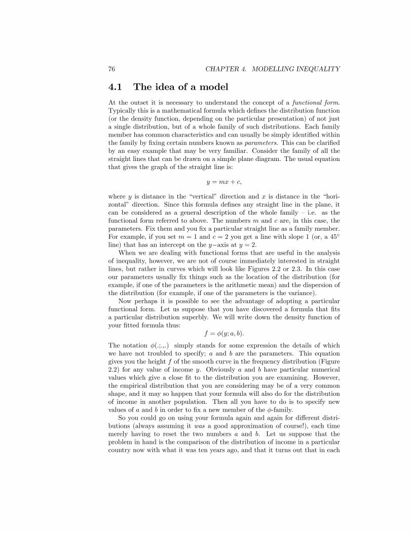
76 CHAPTER 4. MODELLING INEQUALITY
4.1 The idea of a model
At the outset it is necessary to understand the concept of a functional form.Typically this is a mathematical formula which de�nes the distribution function(or the density function, depending on the particular presentation) of not justa single distribution, but of a whole family of such distributions. Each familymember has common characteristics and can usually be simply identi�ed withinthe family by �xing certain numbers known as parameters. This can be clari�edby an easy example that may be very familiar. Consider the family of all thestraight lines that can be drawn on a simple plane diagram. The usual equationthat gives the graph of the straight line is:
y = mx+ c;
where y is distance in the �vertical� direction and x is distance in the �hori-zontal� direction. Since this formula de�nes any straight line in the plane, itcan be considered as a general description of the whole family � i.e. as thefunctional form referred to above. The numbers m and c are, in this case, theparameters. Fix them and you �x a particular straight line as a family member.For example, if you set m = 1 and c = 2 you get a line with slope 1 (or, a 45�
line) that has an intercept on the y�axis at y = 2.When we are dealing with functional forms that are useful in the analysis
of inequality, however, we are not of course immediately interested in straightlines, but rather in curves which will look like Figures 2.2 or 2.3. In this caseour parameters usually �x things such as the location of the distribution (forexample, if one of the parameters is the arithmetic mean) and the dispersion ofthe distribution (for example, if one of the parameters is the variance).Now perhaps it is possible to see the advantage of adopting a particular
functional form. Let us suppose that you have discovered a formula that �tsa particular distribution superbly. We will write down the density function ofyour �tted formula thus:
f = �(y; a; b):
The notation �(.;.,.) simply stands for some expression the details of whichwe have not troubled to specify; a and b are the parameters. This equationgives you the height f of the smooth curve in the frequency distribution (Figure2.2) for any value of income y. Obviously a and b have particular numericalvalues which give a close �t to the distribution you are examining. However,the empirical distribution that you are considering may be of a very commonshape, and it may so happen that your formula will also do for the distributionof income in another population. Then all you have to do is to specify newvalues of a and b in order to �x a new member of the �-family.So you could go on using your formula again and again for di¤erent distri-
butions (always assuming it was a good approximation of course!), each timemerely having to reset the two numbers a and b. Let us suppose that theproblem in hand is the comparison of the distribution of income in a particularcountry now with what it was ten years ago, and that it turns out that in each
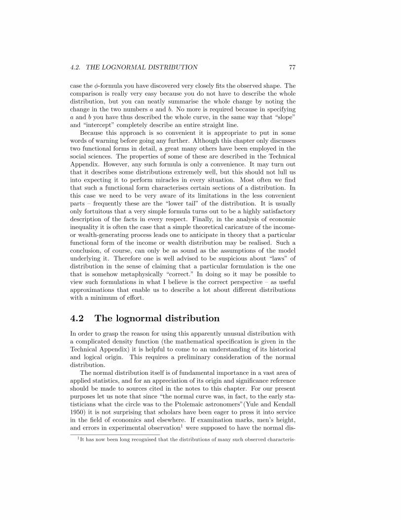
4.2. THE LOGNORMAL DISTRIBUTION 77
case the �-formula you have discovered very closely �ts the observed shape. Thecomparison is really very easy because you do not have to describe the wholedistribution, but you can neatly summarise the whole change by noting thechange in the two numbers a and b. No more is required because in specifyinga and b you have thus described the whole curve, in the same way that �slope�and �intercept�completely describe an entire straight line.Because this approach is so convenient it is appropriate to put in some
words of warning before going any further. Although this chapter only discussestwo functional forms in detail, a great many others have been employed in thesocial sciences. The properties of some of these are described in the TechnicalAppendix. However, any such formula is only a convenience. It may turn outthat it describes some distributions extremely well, but this should not lull usinto expecting it to perform miracles in every situation. Most often we �ndthat such a functional form characterises certain sections of a distribution. Inthis case we need to be very aware of its limitations in the less convenientparts � frequently these are the �lower tail� of the distribution. It is usuallyonly fortuitous that a very simple formula turns out to be a highly satisfactorydescription of the facts in every respect. Finally, in the analysis of economicinequality it is often the case that a simple theoretical caricature of the income-or wealth-generating process leads one to anticipate in theory that a particularfunctional form of the income or wealth distribution may be realised. Such aconclusion, of course, can only be as sound as the assumptions of the modelunderlying it. Therefore one is well advised to be suspicious about �laws� ofdistribution in the sense of claiming that a particular formulation is the onethat is somehow metaphysically �correct.� In doing so it may be possible toview such formulations in what I believe is the correct perspective �as usefulapproximations that enable us to describe a lot about di¤erent distributionswith a minimum of e¤ort.
4.2 The lognormal distribution
In order to grasp the reason for using this apparently unusual distribution witha complicated density function (the mathematical speci�cation is given in theTechnical Appendix) it is helpful to come to an understanding of its historicaland logical origin. This requires a preliminary consideration of the normaldistribution.The normal distribution itself is of fundamental importance in a vast area of
applied statistics, and for an appreciation of its origin and signi�cance referenceshould be made to sources cited in the notes to this chapter. For our presentpurposes let us note that since �the normal curve was, in fact, to the early sta-tisticians what the circle was to the Ptolemaic astronomers�(Yule and Kendall1950) it is not surprising that scholars have been eager to press it into servicein the �eld of economics and elsewhere. If examination marks, men�s height,and errors in experimental observation1 were supposed to have the normal dis-
1 It has now been long recognised that the distributions of many such observed characteris-
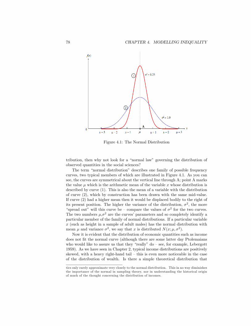
78 CHAPTER 4. MODELLING INEQUALITY
Figure 4.1: The Normal Distribution
tribution, then why not look for a �normal law�governing the distribution ofobserved quantities in the social sciences?The term �normal distribution�describes one family of possible frequency
curves, two typical members of which are illustrated in Figure 4.1. As you cansee, the curves are symmetrical about the vertical line through A; point A marksthe value � which is the arithmetic mean of the variable x whose distribution isdescribed by curve (1). This is also the mean of a variable with the distributionof curve (2), which by construction has been drawn with the same mid-value.If curve (2) had a higher mean then it would be displaced bodily to the right ofits present position. The higher the variance of the distribution, �2, the more�spread out�will this curve be �compare the values of �2 for the two curves.The two numbers �,�2 are the curves�parameters and so completely identify aparticular member of the family of normal distributions. If a particular variablex (such as height in a sample of adult males) has the normal distribution withmean � and variance �2, we say that x is distributed N(x;�; �2).Now it is evident that the distribution of economic quantities such as income
does not �t the normal curve (although there are some latter day Ptolemaianswho would like to assure us that they �really�do �see, for example, Lebergott1959). As we have seen in Chapter 2, typical income distributions are positivelyskewed, with a heavy right-hand tail �this is even more noticeable in the caseof the distribution of wealth. Is there a simple theoretical distribution that
tics only rarely approximate very closely to the normal distribution. This in no way diminishesthe importance of the normal in sampling theory, nor in understanding the historical originof much of the thought concerning the distribution of incomes.
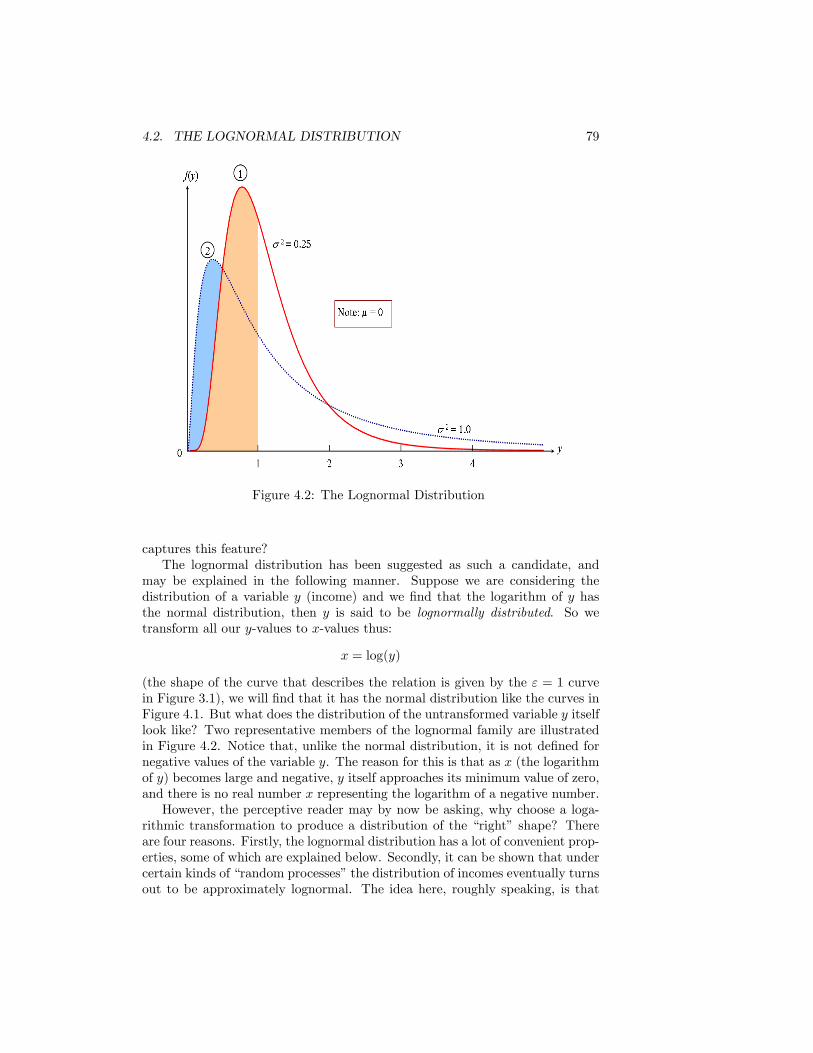
4.2. THE LOGNORMAL DISTRIBUTION 79
Figure 4.2: The Lognormal Distribution
captures this feature?The lognormal distribution has been suggested as such a candidate, and
may be explained in the following manner. Suppose we are considering thedistribution of a variable y (income) and we �nd that the logarithm of y hasthe normal distribution, then y is said to be lognormally distributed. So wetransform all our y-values to x-values thus:
x = log(y)
(the shape of the curve that describes the relation is given by the " = 1 curvein Figure 3.1), we will �nd that it has the normal distribution like the curves inFigure 4.1. But what does the distribution of the untransformed variable y itselflook like? Two representative members of the lognormal family are illustratedin Figure 4.2. Notice that, unlike the normal distribution, it is not de�ned fornegative values of the variable y. The reason for this is that as x (the logarithmof y) becomes large and negative, y itself approaches its minimum value of zero,and there is no real number x representing the logarithm of a negative number.However, the perceptive reader may by now be asking, why choose a loga-
rithmic transformation to produce a distribution of the �right� shape? Thereare four reasons. Firstly, the lognormal distribution has a lot of convenient prop-erties, some of which are explained below. Secondly, it can be shown that undercertain kinds of �random processes�the distribution of incomes eventually turnsout to be approximately lognormal. The idea here, roughly speaking, is that
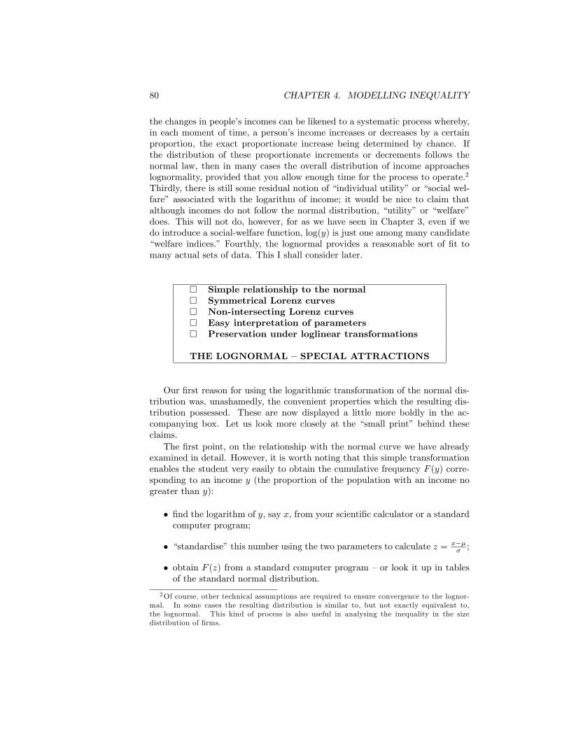
80 CHAPTER 4. MODELLING INEQUALITY
the changes in people�s incomes can be likened to a systematic process whereby,in each moment of time, a person�s income increases or decreases by a certainproportion, the exact proportionate increase being determined by chance. Ifthe distribution of these proportionate increments or decrements follows thenormal law, then in many cases the overall distribution of income approacheslognormality, provided that you allow enough time for the process to operate.2
Thirdly, there is still some residual notion of �individual utility�or �social wel-fare� associated with the logarithm of income; it would be nice to claim thatalthough incomes do not follow the normal distribution, �utility�or �welfare�does. This will not do, however, for as we have seen in Chapter 3, even if wedo introduce a social-welfare function, log(y) is just one among many candidate�welfare indices.� Fourthly, the lognormal provides a reasonable sort of �t tomany actual sets of data. This I shall consider later.
� Simple relationship to the normal� Symmetrical Lorenz curves� Non-intersecting Lorenz curves� Easy interpretation of parameters� Preservation under loglinear transformations
THE LOGNORMAL �SPECIAL ATTRACTIONS
Our �rst reason for using the logarithmic transformation of the normal dis-tribution was, unashamedly, the convenient properties which the resulting dis-tribution possessed. These are now displayed a little more boldly in the ac-companying box. Let us look more closely at the �small print� behind theseclaims.The �rst point, on the relationship with the normal curve we have already
examined in detail. However, it is worth noting that this simple transformationenables the student very easily to obtain the cumulative frequency F (y) corre-sponding to an income y (the proportion of the population with an income nogreater than y):
� �nd the logarithm of y, say x, from your scienti�c calculator or a standardcomputer program;
� �standardise�this number using the two parameters to calculate z = x��� ;
� obtain F (z) from a standard computer program �or look it up in tablesof the standard normal distribution.
2Of course, other technical assumptions are required to ensure convergence to the lognor-mal. In some cases the resulting distribution is similar to, but not exactly equivalent to,the lognormal. This kind of process is also useful in analysing the inequality in the sizedistribution of �rms.
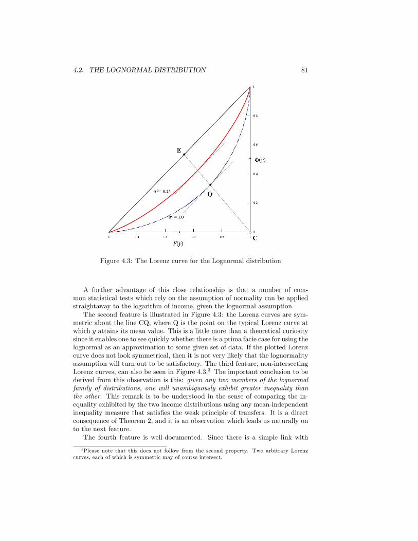
4.2. THE LOGNORMAL DISTRIBUTION 81
Figure 4.3: The Lorenz curve for the Lognormal distribution
A further advantage of this close relationship is that a number of com-mon statistical tests which rely on the assumption of normality can be appliedstraightaway to the logarithm of income, given the lognormal assumption.The second feature is illustrated in Figure 4.3: the Lorenz curves are sym-
metric about the line CQ, where Q is the point on the typical Lorenz curve atwhich y attains its mean value. This is a little more than a theoretical curiositysince it enables one to see quickly whether there is a prima facie case for using thelognormal as an approximation to some given set of data. If the plotted Lorenzcurve does not look symmetrical, then it is not very likely that the lognormalityassumption will turn out to be satisfactory. The third feature, non-intersectingLorenz curves, can also be seen in Figure 4.3.3 The important conclusion to bederived from this observation is this: given any two members of the lognormalfamily of distributions, one will unambiguously exhibit greater inequality thanthe other. This remark is to be understood in the sense of comparing the in-equality exhibited by the two income distributions using any mean-independentinequality measure that satis�es the weak principle of transfers. It is a directconsequence of Theorem 2, and it is an observation which leads us naturally onto the next feature.The fourth feature is well-documented. Since there is a simple link with
3Please note that this does not follow from the second property. Two arbitrary Lorenzcurves, each of which is symmetric may of course intersect.
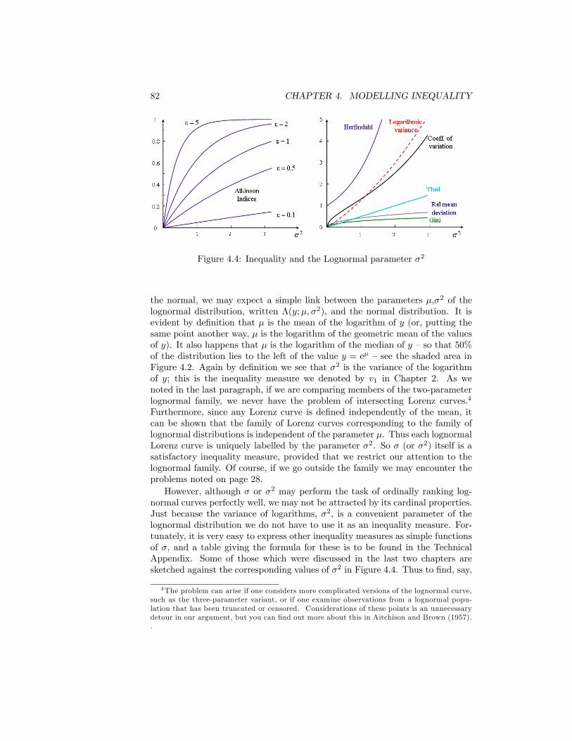
82 CHAPTER 4. MODELLING INEQUALITY
Figure 4.4: Inequality and the Lognormal parameter �2
the normal, we may expect a simple link between the parameters �,�2 of thelognormal distribution, written �(y;�; �2), and the normal distribution. It isevident by de�nition that � is the mean of the logarithm of y (or, putting thesame point another way, � is the logarithm of the geometric mean of the valuesof y). It also happens that � is the logarithm of the median of y �so that 50%of the distribution lies to the left of the value y = e� �see the shaded area inFigure 4.2. Again by de�nition we see that �2 is the variance of the logarithmof y; this is the inequality measure we denoted by v1 in Chapter 2. As wenoted in the last paragraph, if we are comparing members of the two-parameterlognormal family, we never have the problem of intersecting Lorenz curves.4
Furthermore, since any Lorenz curve is de�ned independently of the mean, itcan be shown that the family of Lorenz curves corresponding to the family oflognormal distributions is independent of the parameter �. Thus each lognormalLorenz curve is uniquely labelled by the parameter �2. So � (or �2) itself is asatisfactory inequality measure, provided that we restrict our attention to thelognormal family. Of course, if we go outside the family we may encounter theproblems noted on page 28.However, although � or �2 may perform the task of ordinally ranking log-
normal curves perfectly well, we may not be attracted by its cardinal properties.Just because the variance of logarithms, �2, is a convenient parameter of thelognormal distribution we do not have to use it as an inequality measure. For-tunately, it is very easy to express other inequality measures as simple functionsof �, and a table giving the formula for these is to be found in the TechnicalAppendix. Some of those which were discussed in the last two chapters aresketched against the corresponding values of �2 in Figure 4.4. Thus to �nd, say,
4The problem can arise if one considers more complicated versions of the lognormal curve,such as the three-parameter variant, or if one examine observations from a lognormal popu-lation that has been truncated or censored. Considerations of these points is an unnecessarydetour in our argument, but you can �nd out more about this in Aitchison and Brown (1957)..
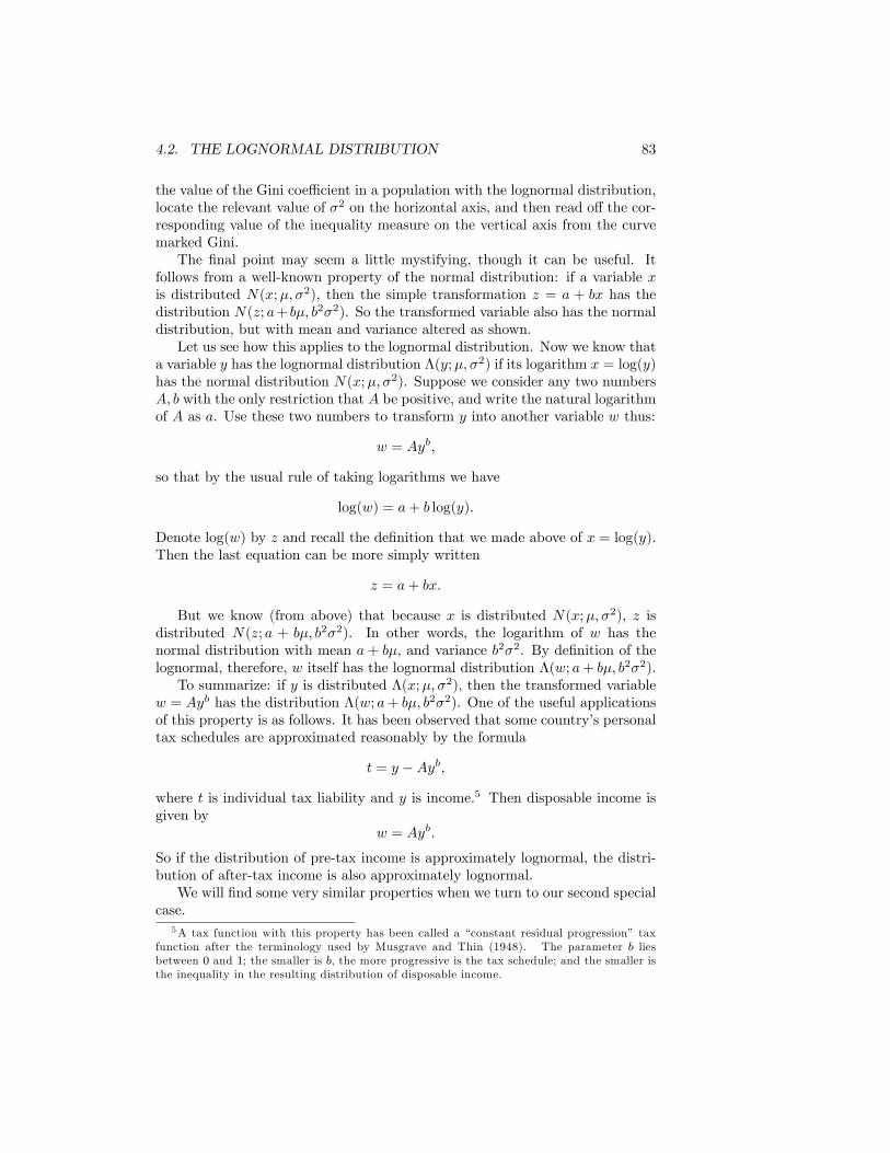
4.2. THE LOGNORMAL DISTRIBUTION 83
the value of the Gini coe¢ cient in a population with the lognormal distribution,locate the relevant value of �2 on the horizontal axis, and then read o¤ the cor-responding value of the inequality measure on the vertical axis from the curvemarked Gini.The �nal point may seem a little mystifying, though it can be useful. It
follows from a well-known property of the normal distribution: if a variable xis distributed N(x;�; �2), then the simple transformation z = a + bx has thedistribution N(z; a+ b�; b2�2). So the transformed variable also has the normaldistribution, but with mean and variance altered as shown.Let us see how this applies to the lognormal distribution. Now we know that
a variable y has the lognormal distribution �(y;�; �2) if its logarithm x = log(y)has the normal distribution N(x;�; �2). Suppose we consider any two numbersA; b with the only restriction that A be positive, and write the natural logarithmof A as a. Use these two numbers to transform y into another variable w thus:
w = Ayb;
so that by the usual rule of taking logarithms we have
log(w) = a+ b log(y):
Denote log(w) by z and recall the de�nition that we made above of x = log(y).Then the last equation can be more simply written
z = a+ bx:
But we know (from above) that because x is distributed N(x;�; �2), z isdistributed N(z; a + b�; b2�2). In other words, the logarithm of w has thenormal distribution with mean a + b�, and variance b2�2. By de�nition of thelognormal, therefore, w itself has the lognormal distribution �(w; a+ b�; b2�2).To summarize: if y is distributed �(x;�; �2), then the transformed variable
w = Ayb has the distribution �(w; a+ b�; b2�2). One of the useful applicationsof this property is as follows. It has been observed that some country�s personaltax schedules are approximated reasonably by the formula
t = y �Ayb;
where t is individual tax liability and y is income.5 Then disposable income isgiven by
w = Ayb:
So if the distribution of pre-tax income is approximately lognormal, the distri-bution of after-tax income is also approximately lognormal.We will �nd some very similar properties when we turn to our second special
case.5A tax function with this property has been called a �constant residual progression� tax
function after the terminology used by Musgrave and Thin (1948). The parameter b liesbetween 0 and 1; the smaller is b, the more progressive is the tax schedule; and the smaller isthe inequality in the resulting distribution of disposable income.
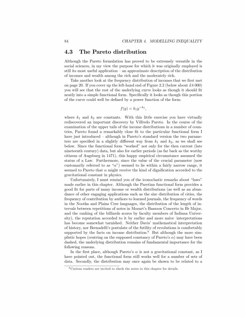
84 CHAPTER 4. MODELLING INEQUALITY
4.3 The Pareto distribution
Although the Pareto formulation has proved to be extremely versatile in thesocial sciences, in my view the purpose for which it was originally employed isstill its most useful application �an approximate description of the distributionof incomes and wealth among the rich and the moderately rich.Take another look at the frequency distribution of incomes that we �rst met
on page 20. If you cover up the left-hand end of Figure 2.2 (below about £ 4 000)you will see that the rest of the underlying curve looks as though it should �tneatly into a simple functional form. Speci�cally it looks as though this portionof the curve could well be de�ned by a power function of the form:
f(y) = k1y�k2 ;
where k1 and k2 are constants. With this little exercise you have virtuallyrediscovered an important discovery by Vilfredo Pareto. In the course of theexamination of the upper tails of the income distributions in a number of coun-tries, Pareto found a remarkably close �t to the particular functional form Ihave just introduced �although in Pareto�s standard version the two parame-ters are speci�ed in a slightly di¤erent way from k1 and k2, as we shall seebelow. Since the functional form �worked�not only for the then current (latenineteenth century) data, but also for earlier periods (as far back as the worthycitizens of Augsburg in 1471), this happy empirical circumstance assumed thestatus of a Law. Furthermore, since the value of the crucial parameter (nowcustomarily referred to as ���) seemed to lie within a fairly narrow range, itseemed to Pareto that � might receive the kind of digni�cation accorded to thegravitational constant in physics.Unfortunately, I must remind you of the iconoclastic remarks about �laws�
made earlier in this chapter. Although the Paretian functional form provides agood �t for parts of many income or wealth distributions (as well as an abun-dance of other engaging applications such as the size distribution of cities, thefrequency of contribution by authors to learned journals, the frequency of wordsin the Nootka and Plains Cree languages, the distribution of the length of in-tervals between repetitions of notes in Mozart�s Bassoon Concerto in B[ Major,and the ranking of the billiards scores by faculty members of Indiana Univer-sity), the reputation accorded to it by earlier and more naive interpretationshas become somewhat tarnished. Neither Davis�mathematical interpretationof history, nor Bernadelli�s postulate of the futility of revolutions is comfortablysupported by the facts on income distribution.6 But although the more sim-plistic hopes (centring on the supposed constancy of Pareto�s �) may have beendashed, the underlying distribution remains of fundamental importance for thefollowing reasons.In the �rst place, although Pareto�s � is not a gravitational constant, as I
have pointed out, the functional form still works well for a number of sets ofdata. Secondly, the distribution may once again be shown to be related to a
6Curious readers are invited to check the notes to this chapter for details.
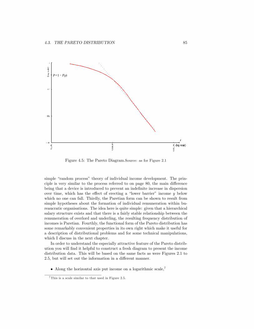
4.3. THE PARETO DISTRIBUTION 85
Figure 4.5: The Pareto Diagram.Source: as for Figure 2.1
simple �random process� theory of individual income development. The prin-ciple is very similar to the process referred to on page 80, the main di¤erencebeing that a device is introduced to prevent an inde�nite increase in dispersionover time, which has the e¤ect of erecting a �lower barrier� income y belowwhich no one can fall. Thirdly, the Paretian form can be shown to result fromsimple hypotheses about the formation of individual remuneration within bu-reaucratic organisations. The idea here is quite simple: given that a hierarchicalsalary structure exists and that there is a fairly stable relationship between theremuneration of overlord and underling, the resulting frequency distribution ofincomes is Paretian. Fourthly, the functional form of the Pareto distribution hassome remarkably convenient properties in its own right which make it useful fora description of distributional problems and for some technical manipulations,which I discuss in the next chapter.In order to understand the especially attractive feature of the Pareto distrib-
ution you will �nd it helpful to construct a fresh diagram to present the incomedistribution data. This will be based on the same facts as were Figures 2.1 to2.5, but will set out the information in a di¤erent manner.
� Along the horizontal axis put income on a logarithmic scale,7
7This is a scale similar to that used in Figure 2.5.
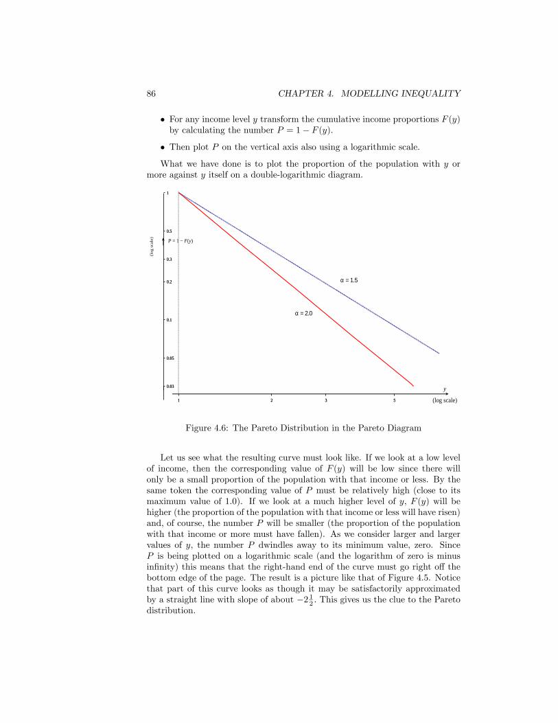
86 CHAPTER 4. MODELLING INEQUALITY
� For any income level y transform the cumulative income proportions F (y)by calculating the number P = 1� F (y).
� Then plot P on the vertical axis also using a logarithmic scale.
What we have done is to plot the proportion of the population with y ormore against y itself on a double-logarithmic diagram.
1 2 3 51 2 3 5
0.03
0.05
0.1
0.2
0.3
0.5
1
0.03
0.05
0.1
0.2
0.3
0.5
1
P = 1 − F(y)
(log
sca
le)
α = 1.5
α = 2.0
y
(log scale)
Figure 4.6: The Pareto Distribution in the Pareto Diagram
Let us see what the resulting curve must look like. If we look at a low levelof income, then the corresponding value of F (y) will be low since there willonly be a small proportion of the population with that income or less. By thesame token the corresponding value of P must be relatively high (close to itsmaximum value of 1:0). If we look at a much higher level of y; F (y) will behigher (the proportion of the population with that income or less will have risen)and, of course, the number P will be smaller (the proportion of the populationwith that income or more must have fallen). As we consider larger and largervalues of y, the number P dwindles away to its minimum value, zero. SinceP is being plotted on a logarithmic scale (and the logarithm of zero is minusin�nity) this means that the right-hand end of the curve must go right o¤ thebottom edge of the page. The result is a picture like that of Figure 4.5. Noticethat part of this curve looks as though it may be satisfactorily approximatedby a straight line with slope of about �2 12 : This gives us the clue to the Paretodistribution.
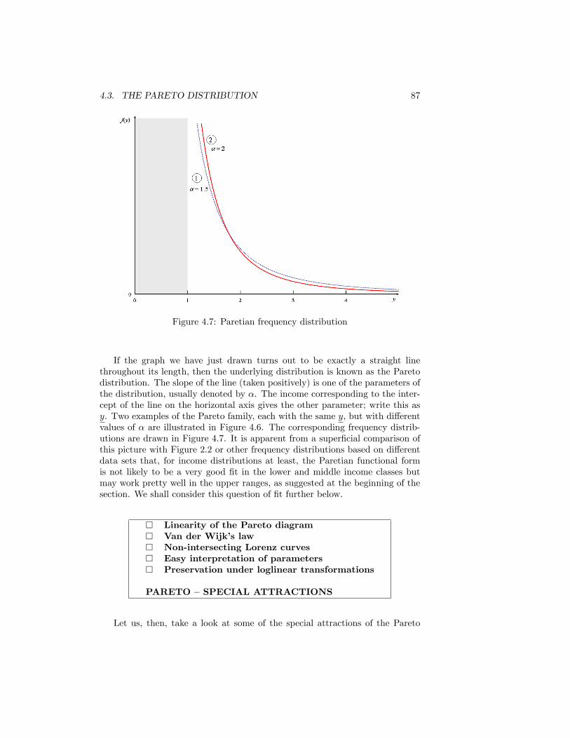
4.3. THE PARETO DISTRIBUTION 87
Figure 4.7: Paretian frequency distribution
If the graph we have just drawn turns out to be exactly a straight linethroughout its length, then the underlying distribution is known as the Paretodistribution. The slope of the line (taken positively) is one of the parameters ofthe distribution, usually denoted by �. The income corresponding to the inter-cept of the line on the horizontal axis gives the other parameter; write this asy. Two examples of the Pareto family, each with the same y, but with di¤erentvalues of � are illustrated in Figure 4.6. The corresponding frequency distrib-utions are drawn in Figure 4.7. It is apparent from a super�cial comparison ofthis picture with Figure 2.2 or other frequency distributions based on di¤erentdata sets that, for income distributions at least, the Paretian functional formis not likely to be a very good �t in the lower and middle income classes butmay work pretty well in the upper ranges, as suggested at the beginning of thesection. We shall consider this question of �t further below.
� Linearity of the Pareto diagram� Van der Wijk�s law� Non-intersecting Lorenz curves� Easy interpretation of parameters� Preservation under loglinear transformations
PARETO �SPECIAL ATTRACTIONS
Let us, then, take a look at some of the special attractions of the Pareto
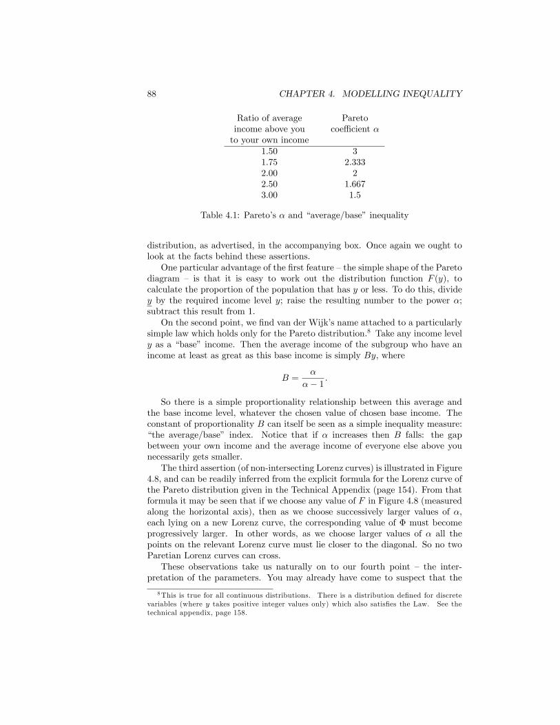
88 CHAPTER 4. MODELLING INEQUALITY
Ratio of average Paretoincome above you coe¢ cient �to your own income
1.50 31.75 2.3332.00 22.50 1.6673.00 1.5
Table 4.1: Pareto�s � and �average/base�inequality
distribution, as advertised, in the accompanying box. Once again we ought tolook at the facts behind these assertions.One particular advantage of the �rst feature �the simple shape of the Pareto
diagram � is that it is easy to work out the distribution function F (y), tocalculate the proportion of the population that has y or less. To do this, dividey by the required income level y; raise the resulting number to the power �;subtract this result from 1.On the second point, we �nd van der Wijk�s name attached to a particularly
simple law which holds only for the Pareto distribution.8 Take any income levely as a �base� income. Then the average income of the subgroup who have anincome at least as great as this base income is simply By, where
B =�
�� 1 :
So there is a simple proportionality relationship between this average andthe base income level, whatever the chosen value of chosen base income. Theconstant of proportionality B can itself be seen as a simple inequality measure:�the average/base� index. Notice that if � increases then B falls: the gapbetween your own income and the average income of everyone else above younecessarily gets smaller.The third assertion (of non-intersecting Lorenz curves) is illustrated in Figure
4.8, and can be readily inferred from the explicit formula for the Lorenz curve ofthe Pareto distribution given in the Technical Appendix (page 154). From thatformula it may be seen that if we choose any value of F in Figure 4.8 (measuredalong the horizontal axis), then as we choose successively larger values of �,each lying on a new Lorenz curve, the corresponding value of � must becomeprogressively larger. In other words, as we choose larger values of � all thepoints on the relevant Lorenz curve must lie closer to the diagonal. So no twoParetian Lorenz curves can cross.These observations take us naturally on to our fourth point � the inter-
pretation of the parameters. You may already have come to suspect that the
8This is true for all continuous distributions. There is a distribution de�ned for discretevariables (where y takes positive integer values only) which also satis�es the Law. See thetechnical appendix, page 158.

4.3. THE PARETO DISTRIBUTION 89
Figure 4.8: The Lorenz curve for the Pareto distribution
parameter � reveals something about the amount of inequality exhibited by aparticular Pareto distribution. Since it is evident that, within the Pareto family,Lorenz curves associated with higher values of � are closer to the line of perfectequality, it follows that if we compare two Pareto distributions with the samemean, the one with the higher value of � exhibits the less amount of inequalityfor all inequality measures satisfying the weak principle of transfers.9
Once again, just because the parameter � is convenient in the case of thePareto distribution, this does not mean that there is any particular merit inusing it as a measure of equality. We may prefer the cardinal characteristics ofsome other measure, in which case we may compute the alternative measure asa function of � using the table in the Technical Appendix, or using Figure 4.9.This �gure is to be interpreted in a manner very similar to that of Figure 4.4 inthe case of the lognormal distribution. The interpretation of the parameter ycan easily be seen from Figure 4.9, which has been drawn with y set arbitrarilyto one. This parameter may assume any positive (but not zero) value, andgives the lower income limit for which the distribution is de�ned. By a simpleapplication of van der Wijk�s law, putting yourself at minimum income y, it can
9An intuitive argument can be used here. Using Van der Wijk�s law you �nd the gapbetween your own income and the average income of everyone above you diminishes the largeris �: Thus the �unfairness� of the income distribution as perceived by you has diminished.
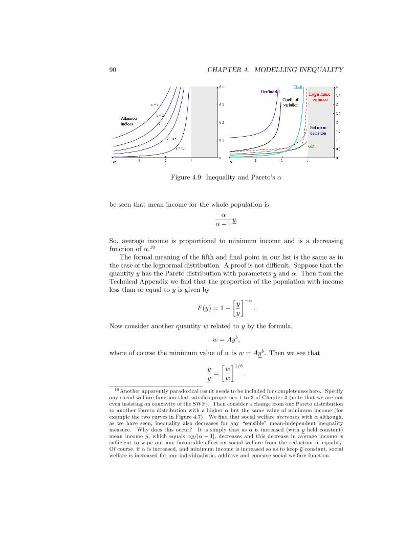
90 CHAPTER 4. MODELLING INEQUALITY
Figure 4.9: Inequality and Pareto�s �
be seen that mean income for the whole population is
�
�� 1y:
So, average income is proportional to minimum income and is a decreasingfunction of �.10
The formal meaning of the �fth and �nal point in our list is the same as inthe case of the lognormal distribution. A proof is not di¢ cult. Suppose that thequantity y has the Pareto distribution with parameters y and �. Then from theTechnical Appendix we �nd that the proportion of the population with incomeless than or equal to y is given by
F (y) = 1��y
y
���:
Now consider another quantity w related to y by the formula,
w = Ayb;
where of course the minimum value of w is w = Ayb. Then we see that
y
y=
�w
w
�1=b:
10Another apparently paradoxical result needs to be included for completeness here. Specifyany social welfare function that satis�es properties 1 to 3 of Chapter 3 (note that we are noteven insisting on concavity of the SWF). Then consider a change from one Pareto distributionto another Pareto distribution with a higher � but the same value of minimum income (forexample the two curves in Figure 4.7). We �nd that social welfare decreases with � although,as we have seen, inequality also decreases for any �sensible� mean-independent inequalitymeasure. Why does this occur? It is simply that as � is increased (with y held constant)mean income �y, which equals �y=[� � 1], decreases and this decrease in average income issu¢ cient to wipe out any favourable e¤ect on social welfare from the reduction in equality.Of course, if � is increased, and minimum income is increased so as to keep �y constant, socialwelfare is increased for any individualistic, additive and concave social welfare function.
4.4. HOW GOOD ARE THE FUNCTIONAL FORMS? 91
Substituting in the formula for F we �nd
F (w) = 1��w
w
���=b:
In other words the transformed variable also has the Pareto distributionwith parameters w and �=b. Therefore we once again have the simple resultthat if pre-tax incomes are distributed according to the Pareto law, and if thetax system is closely approximated by the constant residual progression formula,then post-tax incomes are also distributed according to the Pareto law.
4.4 How good are the functional forms?
An obviously important criterion of suitability of a functional form is that itshould roughly approximate the facts we wish to examine. It is too much tohope that one formula is going to �t some of the data all of the time or all of thedata some of the time, but if it �ts a non-negligible amount of the data a non-negligible amount of the time then the mathematical convenience of the formulamay count for a great deal. One immediate di¢ culty is that the suitability ofthe functional form will depend on the kind of data being analysed. I shall dealwith this by arbitrarily discussing four subject areas which are of particulareconomic interest. In doing so I am giving a mere sketch of the facts which mayprovide those interested with a motivation to enquire further.Aitchison and Brown (1957) argued that the lognormal hypothesis was par-
ticularly appropriate for the distribution of earnings in fairly homogeneous sec-tions of the workforce. Thus, for example, in British agriculture in 1950 we�nd that the distribution of earnings among cowmen, the distribution amonghorsemen, that among stockmen and that among market gardeners proves ineach case to be close to the lognormal. This evidence is also borne out in otherspeci�c sectors of the labour market and in other countries.When we look at more comprehensive populations a di¢ culty arises in that
the aggregate of several distinct lognormal distributions may not itself be lognor-mal. Suppose you have a number of di¤erent subgroups within the population(for example cowmen, horsemen, stockmen, etc.) and within each subgroup thedistribution in the resulting population (all agricultural workers) will only belognormal if, among other things, the dispersion parameter �2 may be takenas uniform throughout the groups. If your lognormal pigmen have a higher �2
than your lognormal tractor drivers, then you are in trouble. Possibly becausethis restrictive condition is not generally satis�ed, systematic departures fromlognormality are evident in many earnings distributions �although it is inter-esting to note that Figure 4.10 illustrates that the lognormal distribution is nota bad approximation for male manual earnings in the UK. Because of this dif-�culty of aggregation Lydall (1968), in attempting to �nd a general descriptionof his �standard distribution� of pretax wages and salaries for all adult non-agricultural workers, makes the following observations. The central part of the
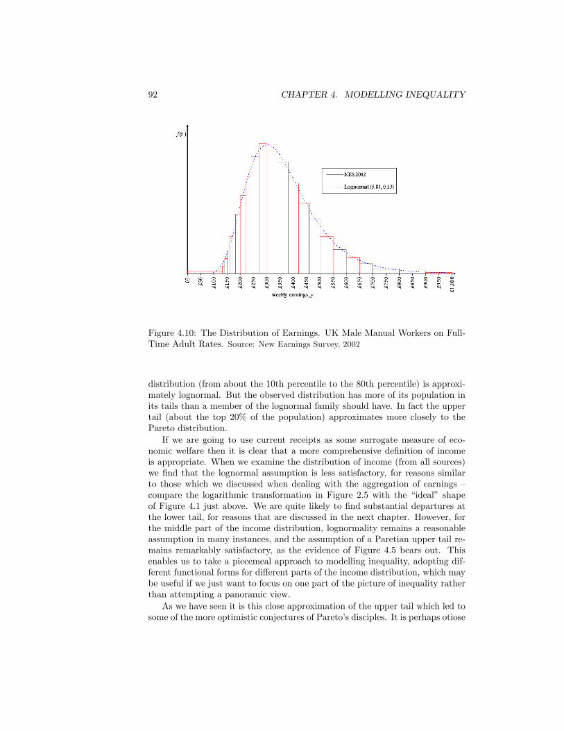
92 CHAPTER 4. MODELLING INEQUALITY
Figure 4.10: The Distribution of Earnings. UK Male Manual Workers on Full-Time Adult Rates. Source: New Earnings Survey, 2002
distribution (from about the 10th percentile to the 80th percentile) is approxi-mately lognormal. But the observed distribution has more of its population inits tails than a member of the lognormal family should have. In fact the uppertail (about the top 20% of the population) approximates more closely to thePareto distribution.If we are going to use current receipts as some surrogate measure of eco-
nomic welfare then it is clear that a more comprehensive de�nition of incomeis appropriate. When we examine the distribution of income (from all sources)we �nd that the lognormal assumption is less satisfactory, for reasons similarto those which we discussed when dealing with the aggregation of earnings �compare the logarithmic transformation in Figure 2.5 with the �ideal� shapeof Figure 4.1 just above. We are quite likely to �nd substantial departures atthe lower tail, for reasons that are discussed in the next chapter. However, forthe middle part of the income distribution, lognormality remains a reasonableassumption in many instances, and the assumption of a Paretian upper tail re-mains remarkably satisfactory, as the evidence of Figure 4.5 bears out. Thisenables us to take a piecemeal approach to modelling inequality, adopting dif-ferent functional forms for di¤erent parts of the income distribution, which maybe useful if we just want to focus on one part of the picture of inequality ratherthan attempting a panoramic view.As we have seen it is this close approximation of the upper tail which led to
some of the more optimistic conjectures of Pareto�s disciples. It is perhaps otiose
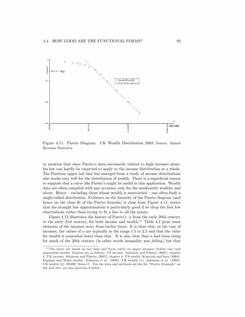
4.4. HOW GOOD ARE THE FUNCTIONAL FORMS? 93
Figure 4.11: Pareto Diagram. UK Wealth Distribution 2003. Source: InlandRevenue Statistics
to mention that since Pareto�s data necessarily related to high incomes alone,his law can hardly be expected to apply to the income distribution as a whole.The Paretian upper tail that has emerged from a study of income distributionsalso works very well for the distribution of wealth. There is a super�cial reasonto suppose that a curve like Pareto�s might be useful in this application. Wealthdata are often compiled with any accuracy only for the moderately wealthy andabove. Hence �excluding those whose wealth is unrecorded �one often �nds asingle-tailed distribution. Evidence on the linearity of the Pareto diagram (andhence on the close �t of the Pareto formula) is clear from Figure 4.11; noticethat the straight line approximation is particularly good if we drop the �rst fewobservations rather than trying to �t a line to all the points.Figure 4.12 illustrates the history of Pareto�s � from the early 20th century
to the early 21st century, for both income and wealth;11 Table 4.2 gives someelements of the incomes story from earlier times. It is clear that, in the case ofincomes, the values of � are typically in the range 1.5 to 2.5 and that the valuefor wealth is somewhat lower than that. It is also clear that � had been risingfor much of the 20th century (in other words inequality was falling) but that
11The series are based on tax data and focus solely on upper incomes (before tax) andsubstantial wealth. Sources are as follows. US income: Atkinson and Piketty (2007), chapter5. UK income: Atkinson and Piketty (2007), chapter 4. US wealth: Kopczuk and Saez (2004).England and Wales wealth: Atkinson et al. (1989). UK wealth (1): Atkinson et al. (1989).UK wealth (2): HMRC Series C . For the data and methods see the �le �Pareto Example�onthe web site; see also question 8 below.
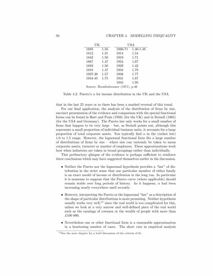
94 CHAPTER 4. MODELLING INEQUALITY
UK USA1688 1.58 1866-71 1.40-1.481812 1.31 1914 1.541843 1.50 1919 1.711867 1.47 1924 1.671893 1.50 1929 1.421918 1.47 1934 1.781937-38 1.57 1938 1.771944-45 1.75 1941 1.87
1945 1.95Source: Bronfenbrenner (1971), p.46
Table 4.2: Pareto�s � for income distribution in the UK and the USA
that in the last 25 years or so there has been a marked reversal of this trend.For our �nal application, the analysis of the distribution of �rms by size,
succinct presentation of the evidence and comparison with the special functionalforms can be found in Hart and Prais (1956) (for the UK) and in Steindl (1965)(for the USA and Germany). The Pareto law only works for a small number of�rms that happen to be very large �but, as Steindl points out, although thisrepresents a small proportion of individual business units, it accounts for a largeproportion of total corporate assets. You typically �nd � in the (rather low)1.0 to 1.5 range. However, the lognormal functional form �ts a large numberof distributions of �rms by size �where size can variously be taken to meancorporate assets, turnover or number of employees. These approximations workbest when industries are taken in broad groupings rather than individually.This perfunctory glimpse of the evidence is perhaps su¢ cient to reinforce
three conclusions which may have suggested themselves earlier in the discussion.
� Neither the Pareto nor the lognormal hypothesis provides a �law�of dis-tribution in the strict sense that one particular member of either familyis an exact model of income or distribution in the long run. In particularit is nonsense to suppose that the Pareto curve (where applicable) shouldremain stable over long periods of history. As it happens, � had beenincreasing nearly everywhere until recently.
� However, interpreting the Pareto or the lognormal �law�as a description ofthe shape of particular distributions is more promising. Neither hypothesisusually works very well,12 since the real world is too complicated for this,unless we look at a very narrow and well-de�ned piece of the real worldsuch as the earnings of cowmen or the wealth of people with more than£ 100 000.
� Nevertheless one or other functional form is a reasonable approximationin a heartening number of cases. The short cuts in empirical analysis
12See the next chapter for a brief discussion of the criteria of �t.
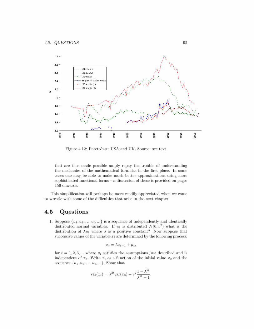
4.5. QUESTIONS 95
Figure 4.12: Pareto�s �: USA and UK. Source: see text
that are thus made possible amply repay the trouble of understandingthe mechanics of the mathematical formulas in the �rst place. In somecases one may be able to make much better approximations using moresophisticated functional forms �a discussion of these is provided on pages156 onwards.
This simpli�cation will perhaps be more readily appreciated when we cometo wrestle with some of the di¢ culties that arise in the next chapter.
4.5 Questions
1. Suppose fu1; u1; ; ::; ut; :::g is a sequence of independently and identicallydistributed normal variables. If ut is distributed N(0; v2) what is thedistribution of �ut where � is a positive constant? Now suppose thatsuccessive values of the variable xt are determined by the following process:
xt = �xt�1 + �t;
for t = 1; 2; 3; ::: where ut satis�es the assumptions just described and isindependent of xt. Write xt as a function of the initial value x0 and thesequence fu1; u1; ; ::; ut; :::g. Show that
var(xt) = �2tvar(x0) + v2 1� �
2t
�2t � 1:
96 CHAPTER 4. MODELLING INEQUALITY
2. Suppose income at time 0, y0, is distributed lognormally. Over a sequenceof periods t = 1; 2; 3; ::: the logarithm of income xt then follows the aboveprocess. Give a simple economic interpretation of what is happening.What will be the distribution of income in period t? Under what condi-tions will the distribution of income converge in the long run? If there isconvergence what is the long-run value of the Gini coe¢ cient?
3. Using the data for the UK 2003 earnings distribution (�NES�on the web-site) compute the mean and the coe¢ cient of variation (i) directly fromthe raw data and (ii) using the �tted lognormal distribution illustrated inFigure 4.10 (use the relevant formula in Table A.2 on page 153).
4. Show that the ��rst guess�at the Pareto distribution given by the formulafor the frequency distribution on page 84 really does correspond to theformula for the distribution function F on page 154 of Appendix A. Whatis the relationship of the constants k1 and k2 to the parameters y and �?
5. Use the formulas given in the Table A.2 and on page 154 to:
(a) derive the generalised Lorenz curve for the Pareto distribution ;
(b) sketch the relationship between coe¢ cient of variation c and � inFigure 4.9;
(c) show why is c unde�ned for � � 2.
6.
(a) Using the data for the UK wealth distribution 2003 (see the �le �IRwealth�on the website) compute the Gini coe¢ cient on the assump-tions (i) that persons not covered by the wealth table are simplyexcluded from the calculation, and (ii) individuals in a given wealthinterval class possess the mean wealth of that interval.
(b) Rework the calculation in part (a) on the alternative assumption thatthe group excluded by assumption (i) actually consists of n personseach with a wealth y0, where n and y0 are positive numbers (chosenby you). What would be reasonable ranges of possible values forthese numbers? How does the computed Gini coe¢ cient vary with nand y0?
7.
(a) Using the same source on the website as in question 6 for the lowerbound of each wealth interval y compute P (as de�ned on page 86)and then use ordinary least squares to �t the equation
log(P ) = �0 + �1 log(y);
then �nd the estimate of Pareto�s �. Use this estimate to computethe Gini coe¢ cient on the hypothesis that the underlying distributionis Paretian.
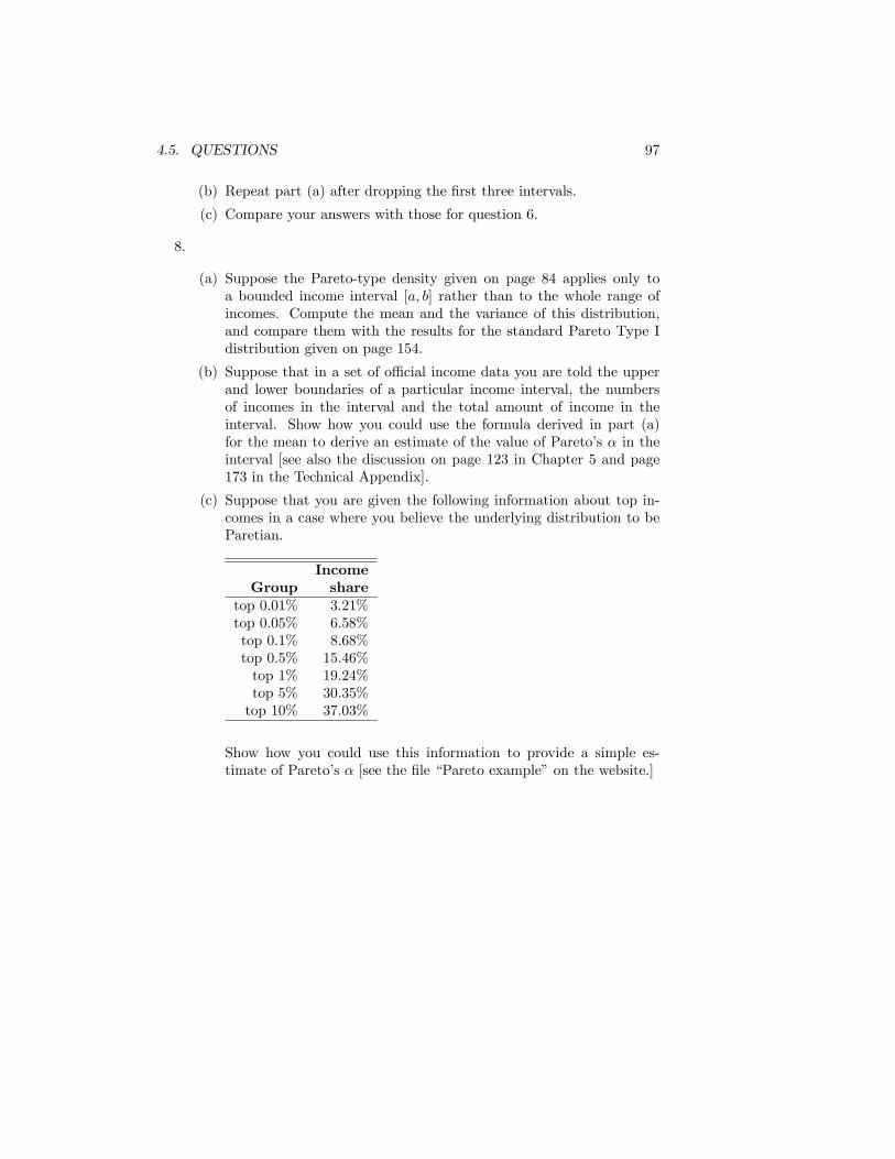
4.5. QUESTIONS 97
(b) Repeat part (a) after dropping the �rst three intervals.
(c) Compare your answers with those for question 6.
8.
(a) Suppose the Pareto-type density given on page 84 applies only toa bounded income interval [a; b] rather than to the whole range ofincomes. Compute the mean and the variance of this distribution,and compare them with the results for the standard Pareto Type Idistribution given on page 154.
(b) Suppose that in a set of o¢ cial income data you are told the upperand lower boundaries of a particular income interval, the numbersof incomes in the interval and the total amount of income in theinterval. Show how you could use the formula derived in part (a)for the mean to derive an estimate of the value of Pareto�s � in theinterval [see also the discussion on page 123 in Chapter 5 and page173 in the Technical Appendix].
(c) Suppose that you are given the following information about top in-comes in a case where you believe the underlying distribution to beParetian.
IncomeGroup share
top 0.01% 3.21%top 0.05% 6.58%top 0.1% 8.68%top 0.5% 15.46%top 1% 19.24%top 5% 30.35%top 10% 37.03%
Show how you could use this information to provide a simple es-timate of Pareto�s � [see the �le �Pareto example�on the website.]

98 CHAPTER 4. MODELLING INEQUALITY

Chapter 5
From Theory to Practice
�What would life be without arithmetic, but a scene of horrors?��Rev. Sydney Smith (1835)
So where do we go now? One perfectly reasonable answer to this would beto return to some of the knotty theoretical issues to which we accorded onlyscant attention earlier.Were we to follow this course, however, we should neglect a large number
of problems which must be wrestled with before our ideas on inequality can beapplied to numbers culled from the real world. In this chapter we shall reviewthese problems in a fairly general way, since many of them arise in the same formwhatever concept of income, wealth or other personal attribute is examined, andwhatever the national or international source from which the data are drawn.
� Data� Computation� Appraising the results� Special functional forms� Interpretation
A CATALOGUE OF PROBLEMS
It is expedient to subdivide the practical problems that we shall meet into�ve broad groups: those that are associated with getting and understanding theoriginal data; those arising from computations using the data; those involvedin an appraisal of the signi�cance of these calculations; the problems connectedwith the use of special functional forms for income distribution; and the inter-pretation of results. Of course many of these problems interact. But we shalltry to deal with them one at a time.
99
100 CHAPTER 5. FROM THEORY TO PRACTICE
5.1 The data
The primary problem to be dealt with by anyone doing quantitative researchinto inequality is that of de�ning the variable y which we have loosely called�income�, and then getting observations on it. In this section we deal with someof these conceptual and practical issues.For certain speci�c problem areas the choice of variable and of source ma-
terial is usually immediately apparent. For example, if one is interested in theinequality of voting power in a political system, the relevant variable is thenumber of seats allocated per thousand of the population (the fraction of arepresentative held by a voting individual); in this situation it is a straightfor-ward step to impute an index of voting power to each member of the electorate.However, in a great many situations where inequality measures are applied, anumber of detailed preliminary considerations about the nature of the �income�variable, y, and the way it is observed in practice are in order. The reasons forthis lie not only in the technique of measurement itself but also in the economicwelfare connotations attached to the variable y. For in such cases we typically�nd that a study of the distribution of income or wealth is being used as a surro-gate for the distribution of an index of individual well-being. We shall considerfurther some of the problems of interpreting the data in this way once we havelooked at the manner in which the �gures are obtained.There are basically two methods of collecting this kind of information:
� You can ask people for it.
� You can make them give it to you.
Neither method is wholly satisfactory since, in the �rst case, some peoplemay choose not to give the information, or may give it incorrectly and, in thesecond case, the legal requirement for information may not correspond exactlyto the data requirements of the social analyst. Let us look more closely at whatis involved.
Method 1: Asking people
This approach is commonly used by those organisations that desire the rawinformation for its own sake. It involves the construction of a carefully strat-i�ed (and thus representative) sample of the population, and then requestingthe members of this sample to give the information that is required about theirincome, wealth, types of asset-holding, spending patterns, household compo-sition, etc. This method is used in the UK�s Family Resources Survey , andin the Current Population Surveys conducted by the US Bureau of the Cen-sus. Obviously a principal di¢ culty is, as I mentioned, that of non-response ormisinformation by those approached in the survey. A common presumption isthat disproportionately many of those refusing to cooperate will be among therich, and thus a potentially signi�cant bias may be introduced into the results.However, the response rate in some of the major surveys is surprisingly good
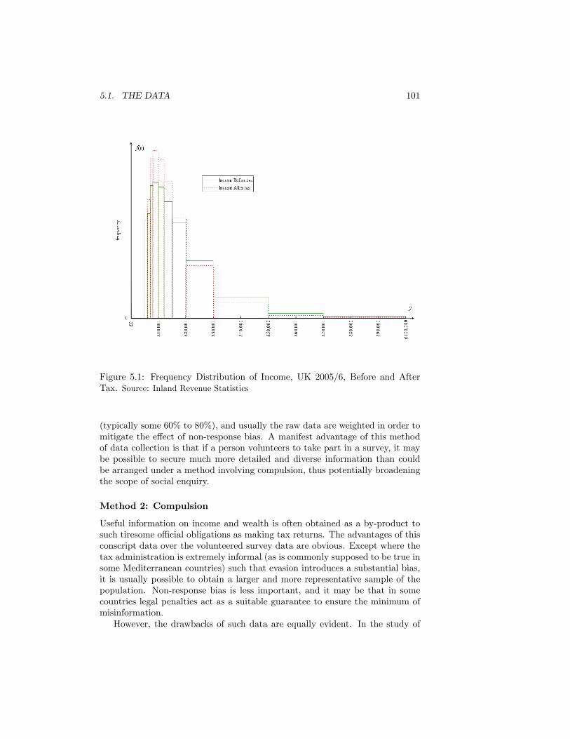
5.1. THE DATA 101
Figure 5.1: Frequency Distribution of Income, UK 2005/6, Before and AfterTax. Source: Inland Revenue Statistics
(typically some 60% to 80%), and usually the raw data are weighted in order tomitigate the e¤ect of non-response bias. A manifest advantage of this methodof data collection is that if a person volunteers to take part in a survey, it maybe possible to secure much more detailed and diverse information than couldbe arranged under a method involving compulsion, thus potentially broadeningthe scope of social enquiry.
Method 2: Compulsion
Useful information on income and wealth is often obtained as a by-product tosuch tiresome o¢ cial obligations as making tax returns. The advantages of thisconscript data over the volunteered survey data are obvious. Except where thetax administration is extremely informal (as is commonly supposed to be true insome Mediterranean countries) such that evasion introduces a substantial bias,it is usually possible to obtain a larger and more representative sample of thepopulation. Non-response bias is less important, and it may be that in somecountries legal penalties act as a suitable guarantee to ensure the minimum ofmisinformation.However, the drawbacks of such data are equally evident. In the study of
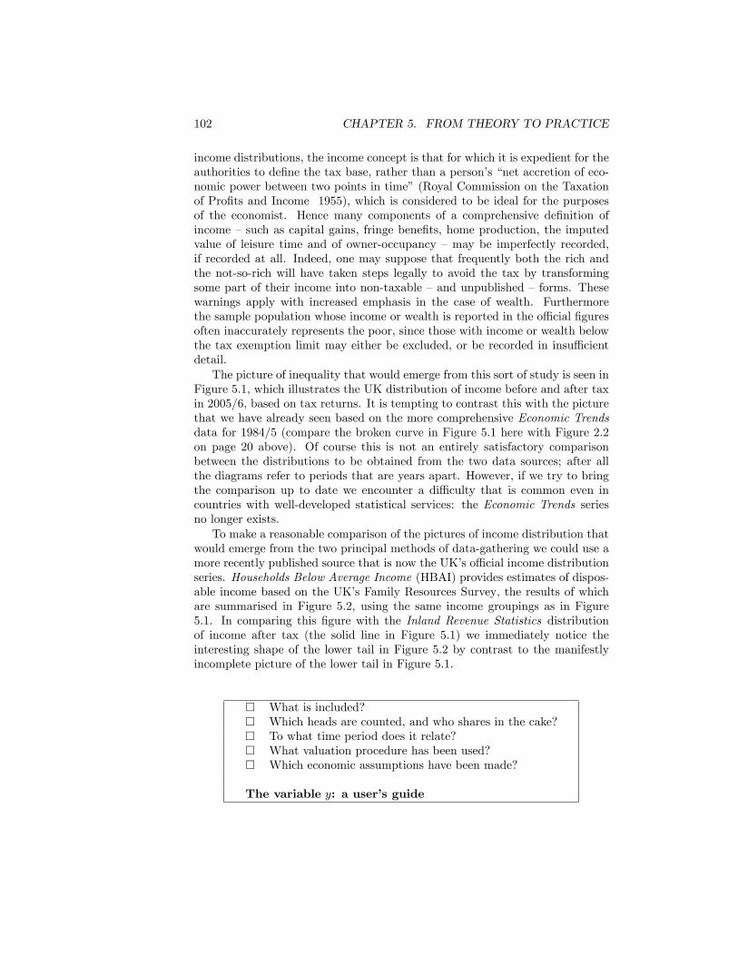
102 CHAPTER 5. FROM THEORY TO PRACTICE
income distributions, the income concept is that for which it is expedient for theauthorities to de�ne the tax base, rather than a person�s �net accretion of eco-nomic power between two points in time�(Royal Commission on the Taxationof Pro�ts and Income 1955), which is considered to be ideal for the purposesof the economist. Hence many components of a comprehensive de�nition ofincome �such as capital gains, fringe bene�ts, home production, the imputedvalue of leisure time and of owner-occupancy �may be imperfectly recorded,if recorded at all. Indeed, one may suppose that frequently both the rich andthe not-so-rich will have taken steps legally to avoid the tax by transformingsome part of their income into non-taxable �and unpublished �forms. Thesewarnings apply with increased emphasis in the case of wealth. Furthermorethe sample population whose income or wealth is reported in the o¢ cial �guresoften inaccurately represents the poor, since those with income or wealth belowthe tax exemption limit may either be excluded, or be recorded in insu¢ cientdetail.The picture of inequality that would emerge from this sort of study is seen in
Figure 5.1, which illustrates the UK distribution of income before and after taxin 2005/6, based on tax returns. It is tempting to contrast this with the picturethat we have already seen based on the more comprehensive Economic Trendsdata for 1984/5 (compare the broken curve in Figure 5.1 here with Figure 2.2on page 20 above). Of course this is not an entirely satisfactory comparisonbetween the distributions to be obtained from the two data sources; after allthe diagrams refer to periods that are years apart. However, if we try to bringthe comparison up to date we encounter a di¢ culty that is common even incountries with well-developed statistical services: the Economic Trends seriesno longer exists.To make a reasonable comparison of the pictures of income distribution that
would emerge from the two principal methods of data-gathering we could use amore recently published source that is now the UK�s o¢ cial income distributionseries. Households Below Average Income (HBAI) provides estimates of dispos-able income based on the UK�s Family Resources Survey, the results of whichare summarised in Figure 5.2, using the same income groupings as in Figure5.1. In comparing this �gure with the Inland Revenue Statistics distributionof income after tax (the solid line in Figure 5.1) we immediately notice theinteresting shape of the lower tail in Figure 5.2 by contrast to the manifestlyincomplete picture of the lower tail in Figure 5.1.
� What is included?� Which heads are counted, and who shares in the cake?� To what time period does it relate?� What valuation procedure has been used?� Which economic assumptions have been made?
The variable y: a user�s guide
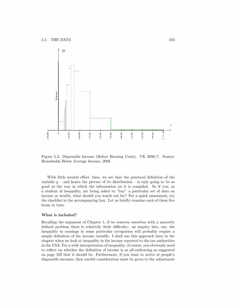
5.1. THE DATA 103
Figure 5.2: Disposable Income (Before Housing Costs). UK 2006/7. Source:Households Below Average Income, 2008
With little mental e¤ort, then, we see that the practical de�nition of thevariable y �and hence the picture of its distribution � is only going to be asgood as the way in which the information on it is compiled. So if you, asa student of inequality, are being asked to �buy� a particular set of data onincome or wealth, what should you watch out for? For a quick assessment, trythe checklist in the accompanying box. Let us brie�y examine each of these �veitems in turn.
What is included?
Recalling the argument of Chapter 1, if we concern ourselves with a narrowlyde�ned problem there is relatively little di¢ culty: an inquiry into, say, theinequality in earnings in some particular occupation will probably require asimple de�nition of the income variable. I shall use this approach later in thechapter when we look at inequality in the income reported to the tax authoritiesin the USA. For a wide interpretation of inequality, of course, you obviously needto re�ect on whether the de�nition of income is as all-embracing as suggestedon page 102 that it should be. Furthermore, if you want to arrive at people�sdisposable incomes, then careful consideration must be given to the adjustment
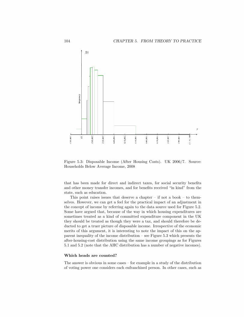
104 CHAPTER 5. FROM THEORY TO PRACTICE
Figure 5.3: Disposable Income (After Housing Costs). UK 2006/7. Source:Households Below Average Income, 2008
that has been made for direct and indirect taxes, for social security bene�tsand other money transfer incomes, and for bene�ts received �in kind�from thestate, such as education.This point raises issues that deserve a chapter � if not a book �to them-
selves. However, we can get a feel for the practical impact of an adjustment inthe concept of income by referring again to the data source used for Figure 5.2.Some have argued that, because of the way in which housing expenditures aresometimes treated as a kind of committed expenditure component in the UKthey should be treated as though they were a tax, and should therefore be de-ducted to get a truer picture of disposable income. Irrespective of the economicmerits of this argument, it is interesting to note the impact of this on the ap-parent inequality of the income distribution �see Figure 5.3 which presents theafter-housing-cost distribution using the same income groupings as for Figures5.1 and 5.2 (note that the AHC distribution has a number of negative incomes).
Which heads are counted?
The answer is obvious in some cases �for example in a study of the distributionof voting power one considers each enfranchised person. In other cases, such as
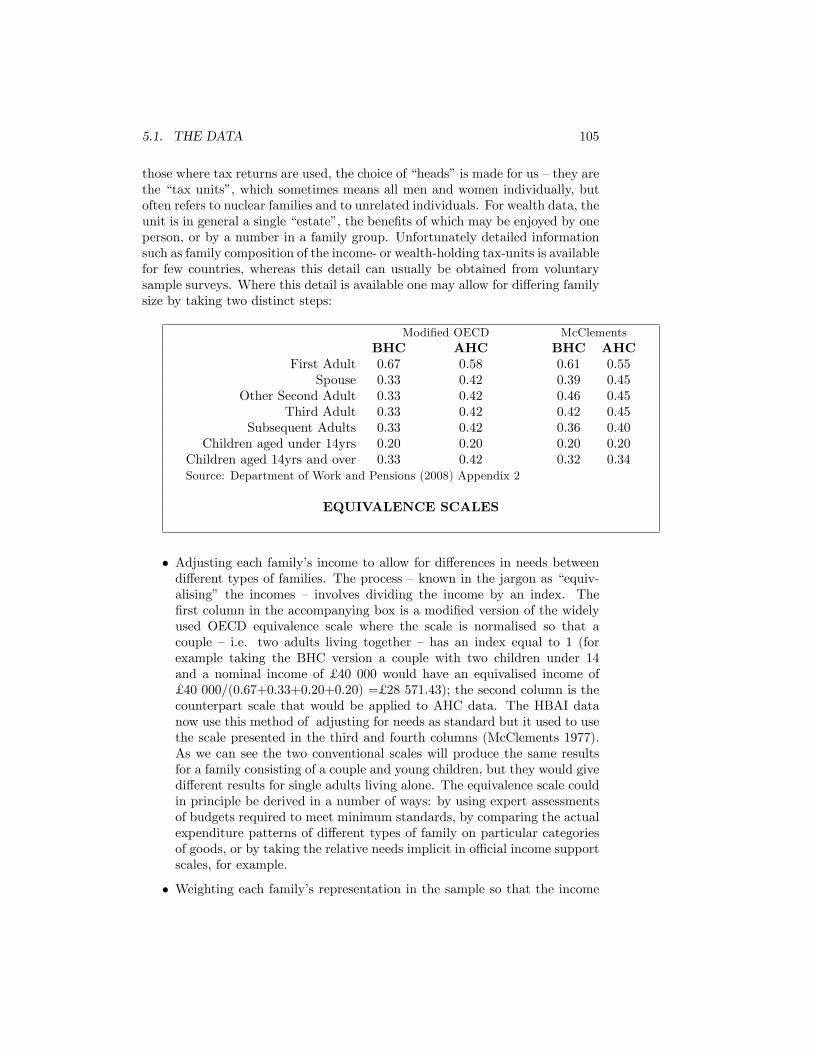
5.1. THE DATA 105
those where tax returns are used, the choice of �heads�is made for us �they arethe �tax units�, which sometimes means all men and women individually, butoften refers to nuclear families and to unrelated individuals. For wealth data, theunit is in general a single �estate�, the bene�ts of which may be enjoyed by oneperson, or by a number in a family group. Unfortunately detailed informationsuch as family composition of the income- or wealth-holding tax-units is availablefor few countries, whereas this detail can usually be obtained from voluntarysample surveys. Where this detail is available one may allow for di¤ering familysize by taking two distinct steps:
Modi�ed OECD McClementsBHC AHC BHC AHC
First Adult 0.67 0.58 0.61 0.55Spouse 0.33 0.42 0.39 0.45
Other Second Adult 0.33 0.42 0.46 0.45Third Adult 0.33 0.42 0.42 0.45
Subsequent Adults 0.33 0.42 0.36 0.40Children aged under 14yrs 0.20 0.20 0.20 0.20
Children aged 14yrs and over 0.33 0.42 0.32 0.34Source: Department of Work and Pensions (2008) Appendix 2
EQUIVALENCE SCALES
� Adjusting each family�s income to allow for di¤erences in needs betweendi¤erent types of families. The process �known in the jargon as �equiv-alising� the incomes � involves dividing the income by an index. The�rst column in the accompanying box is a modi�ed version of the widelyused OECD equivalence scale where the scale is normalised so that acouple � i.e. two adults living together � has an index equal to 1 (forexample taking the BHC version a couple with two children under 14and a nominal income of £ 40 000 would have an equivalised income of£ 40 000/(0.67+0.33+0.20+0.20) =£ 28 571.43); the second column is thecounterpart scale that would be applied to AHC data. The HBAI datanow use this method of adjusting for needs as standard but it used to usethe scale presented in the third and fourth columns (McClements 1977).As we can see the two conventional scales will produce the same resultsfor a family consisting of a couple and young children, but they would givedi¤erent results for single adults living alone. The equivalence scale couldin principle be derived in a number of ways: by using expert assessmentsof budgets required to meet minimum standards, by comparing the actualexpenditure patterns of di¤erent types of family on particular categoriesof goods, or by taking the relative needs implicit in o¢ cial income supportscales, for example.
� Weighting each family�s representation in the sample so that the income
106 CHAPTER 5. FROM THEORY TO PRACTICE
distribution is amongst persons rather than arbitrary family units. Thisis usually done by weighting in proportion to the number of persons inthe family (so the above imaginary family of a married couple and twochildren would be weighted by a factor of four).
There is a variety of alternative assumptions that could be made abouteach of these two steps, and you should be warned that these adjustments cansigni�cantly a¤ect the picture of inequality that emerges (see question 2 for anexample of this).You may well conclude that big enough problems are raised in dealing with
the heterogeneous people who are there in the sample population; but an evenbigger problem is posed by those who aren�t there. This remark applies gener-ally to tax-based data, and particularly to wealth. Only those estates that aresu¢ ciently extensive to attract the attention of the tax authorities are usuallyincluded in the data, and hence there is a large proportion of the populationwhich although not destitute does not appear in the published �gures. Basicallyyou have to do one of three things: leave these people out altogether (and sounderestimate the amount of inequality); include them, but with zero wealth(and so overestimate inequality); or make some estimate of the wealth to be im-puted per capita, by using information from alternative sources on total wealth,or �more ambitiously �by guessing at the distribution among these excludedpersons.
What time period?
Income �as opposed to wealth � is de�ned relative to a particular time unit,and you will generally �nd that measured inequality is noticeably lower if thepersonal income concept relates to a relatively long period than if quite a shorttime interval such as a week or a month is considered. The reason is simply thatpeople�s incomes �uctuate, and the longer you make the time unit, the more you�average out�this volatility. As we noted in Chapter 1 the ultimate extensionof this is to examine the distribution of lifetime average income. However,apart from the conceptual di¢ culties involved there may be practical problemstoo. In some cases longitudinal data sets are available that track the individualincomes over more than one period: this may be used to derive estimates of theinterpersonal distribution of a lifetime average, although fairly sophisticatedtechniques may be required; in some cases su¢ ciently detailed data are just notavailable.
What valuation procedure has been used?
As we have seen there are substantial problems of incorporating non-monetaryitems into the income or wealth aggregate such as income in kind or assetsfor which no easily recognised market price exists. In addition to these prob-lems, the question of the valuation procedure arises particularly when analysingtrends of inequality over time, or in making comparisons between countries.For, when looking at time trends, we must recognise that changes in consumer

5.1. THE DATA 107
goods� prices will a¤ect the purchasing power of the poor and of the rich indi¤erent ways if the spending patterns of these two groups are signi�cantlydi¤erent. In some advanced economies during the recent past, price increaseshappen to have a¤ected necessities disproportionately more than luxuries, andas a consequence looking at inequality purely in money-income terms conceals anincreasing trend in inequality of real purchasing power. If we want to compareinequality within di¤erent countries, or to examine inequality among countriesin per capita income, then even worse trouble lies ahead: one must wrestle withdiverse de�nitions of income, di¤ering relative prices (as in the time trend prob-lem), di¤erent levels and forms of public expenditure, and arti�cial exchangerates �which collectively are giants barring the way to comparability in income-or wealth-valuation.
Which economic assumptions have been made?
To procure certain versions of the income or wealth variable some economicsleight-of-hand is essential, and it is important to grasp the legitimate tricksinvolved. Let us brie�y consider two of the most frequently encountered issues.
First, how are we to allow for people�s reactions to price and income changes?Taxation generally involves distortion of prices �those of commodities, and thevalue of time available for work. Now people�s choices of the amount they workand the amount they save may be a¤ected by changes in these prices, whichmeans in turn that the income distribution itself is a¤ected. So if you want toinfer from the published �gures what the shape of the income distribution wouldbe without government intervention, you must allow for this income response,which in practice usually means �atly ignoring it. This remark applies to thee¤ects of indirect taxation as well as to income tax.
The second issue concerns the assumptions about markets. Time and againone has to sum unlike components in an income or wealth aggregate. To getan overall measure of net worth one adds a person�s current wealth (in terms ofmarketable assets) to a present valuation of future income receipts from othersources. To evaluate a family�s disposable income after all forms of interventionone must include the value of non-monetary government transfers along withmoney income. Either exercise involves not only the selection of prices, as wediscussed above, but usually a tacit assumption about the existence of e¢ ciently-operating markets for capital and for government-provided goods. To see this,note that a person with high future income but low current wealth can onlybe said to be as well o¤ as a person with high current wealth but low incomeprospects if it is possible to borrow from the capital market on the strength ofone�s anticipated high earnings. Taking your cue from the Rev. S. Smith, youmight think that enough �horrors� had been met in just examining the data.But we must press on.
108 CHAPTER 5. FROM THEORY TO PRACTICE
5.2 Computation of the inequality measures
Let us assume that you have decided on the variable y that you wish to use,and the source from which you are going to extract the data. As we shall see,there are some potentially signi�cant problems associated with the arithmeticinvolved in proceedings from a table of raw data to a number giving the realisedvalue of an inequality measure. We proceed by describing a number of inequalitymeasures that were introduced in Chapters 2 and 3 in a formal but economicalmanner, and then using this presentation to explore the practical di¢ culties.Suppose that for a particular population you know the theoretical density
function f(y), which gives the proportion of the population that has an incomein the in�nitesimal interval y to y+ dy.1 This function is de�ned so that if it issummed over the entire income range the result is exactly one; formally:Z 1
0
f(y)dy = 1:
Now let us suppose that the desired inequality measure, or an ordinallyequivalent transformation of the desired inequality measure, can be written inthe following way, which we shall refer to as the basic form:
J =
Z 1
0
h(y)f(y)dy;
where h(:) is an evaluation function �some function of y that we have yet tospecify. It so happens that nearly every inequality measure that is of interest,except the Gini coe¢ cient, can be shown to be ordinally equivalent to some-thing that can be written in the basic form �mathematically inclined readersare invited to check this from Tables A.1 and A.2 in the Technical Appendix.Some can be written exactly in the basic form �for example the relative meandeviation, for which we would have the following evaluation function
h(y) =
����yy � 1����
or Theil�s inequality measure for which we �nd
h(y) =y
ylog
�y
y
�:
1For those who are uneasy about integration an intuitive description may help. Supposethat you have a diagram of a smooth curve �(y); drawn with y measured �horizontally� and� �vertically�. Then
R ba �(y)dy means the area under the curve, above the horizontal axis and
bounded on either side by the vertical lines y = a and y = b. Thus in Figure 2.2R 12;50010;000 �(y)dy
means the area between the smooth curve and the line OF that also lies between the pointsmarked 10,000 and 12,500. Instead of working out just the one single shaded rectangle it isas though we caluclated the area of lots of rectangles of tiny base width made to �t under thecurve along this small interval. The �
R�sign can be taken as something quite similar to the
summation sign ��":
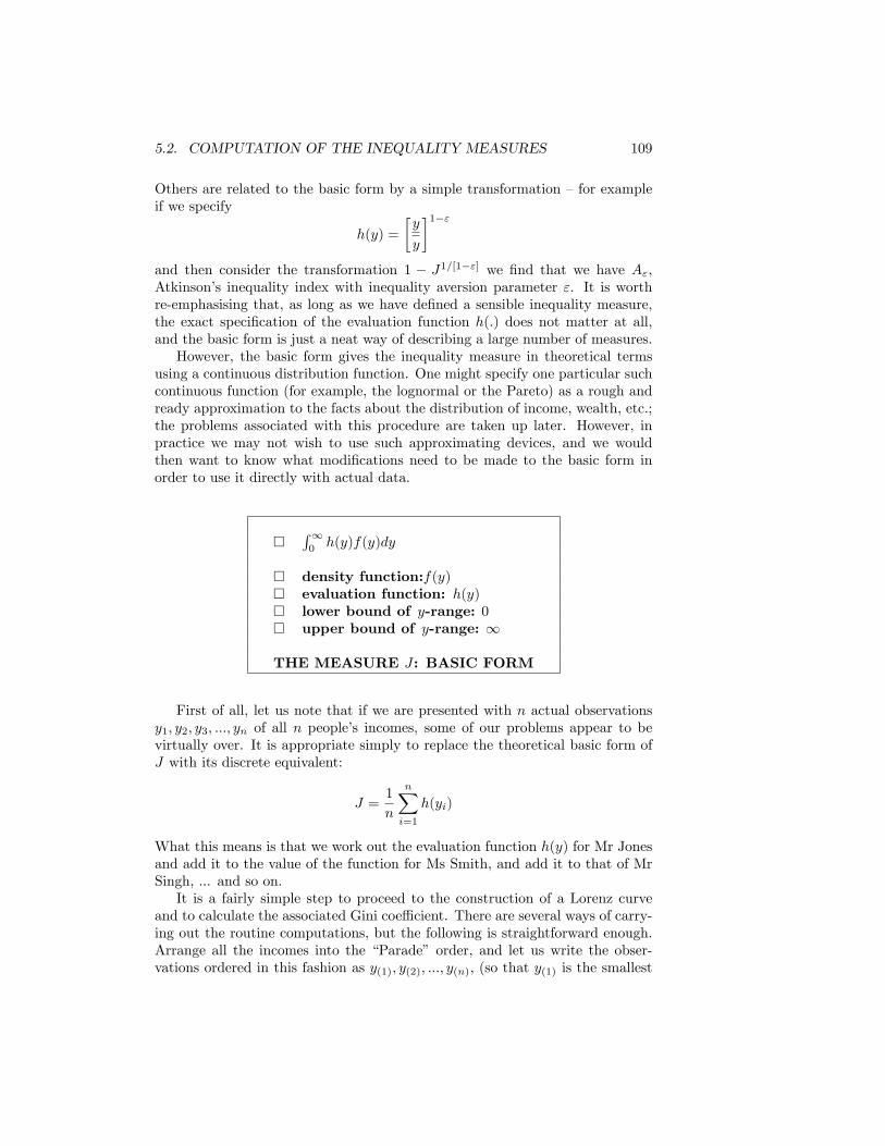
5.2. COMPUTATION OF THE INEQUALITY MEASURES 109
Others are related to the basic form by a simple transformation �for exampleif we specify
h(y) =
�y
y
�1�"and then consider the transformation 1 � J1=[1�"] we �nd that we have A",Atkinson�s inequality index with inequality aversion parameter ". It is worthre-emphasising that, as long as we have de�ned a sensible inequality measure,the exact speci�cation of the evaluation function h(:) does not matter at all,and the basic form is just a neat way of describing a large number of measures.However, the basic form gives the inequality measure in theoretical terms
using a continuous distribution function. One might specify one particular suchcontinuous function (for example, the lognormal or the Pareto) as a rough andready approximation to the facts about the distribution of income, wealth, etc.;the problems associated with this procedure are taken up later. However, inpractice we may not wish to use such approximating devices, and we wouldthen want to know what modi�cations need to be made to the basic form inorder to use it directly with actual data.
�R10h(y)f(y)dy
� density function:f(y)� evaluation function: h(y)� lower bound of y-range: 0� upper bound of y-range: 1
THE MEASURE J : BASIC FORM
First of all, let us note that if we are presented with n actual observationsy1; y2; y3; :::; yn of all n people�s incomes, some of our problems appear to bevirtually over. It is appropriate simply to replace the theoretical basic form ofJ with its discrete equivalent:
J =1
n
nXi=1
h(yi)
What this means is that we work out the evaluation function h(y) for Mr Jonesand add it to the value of the function for Ms Smith, and add it to that of MrSingh, ... and so on.It is a fairly simple step to proceed to the construction of a Lorenz curve
and to calculate the associated Gini coe¢ cient. There are several ways of carry-ing out the routine computations, but the following is straightforward enough.Arrange all the incomes into the �Parade� order, and let us write the obser-vations ordered in this fashion as y(1); y(2); :::; y(n); (so that y(1) is the smallest
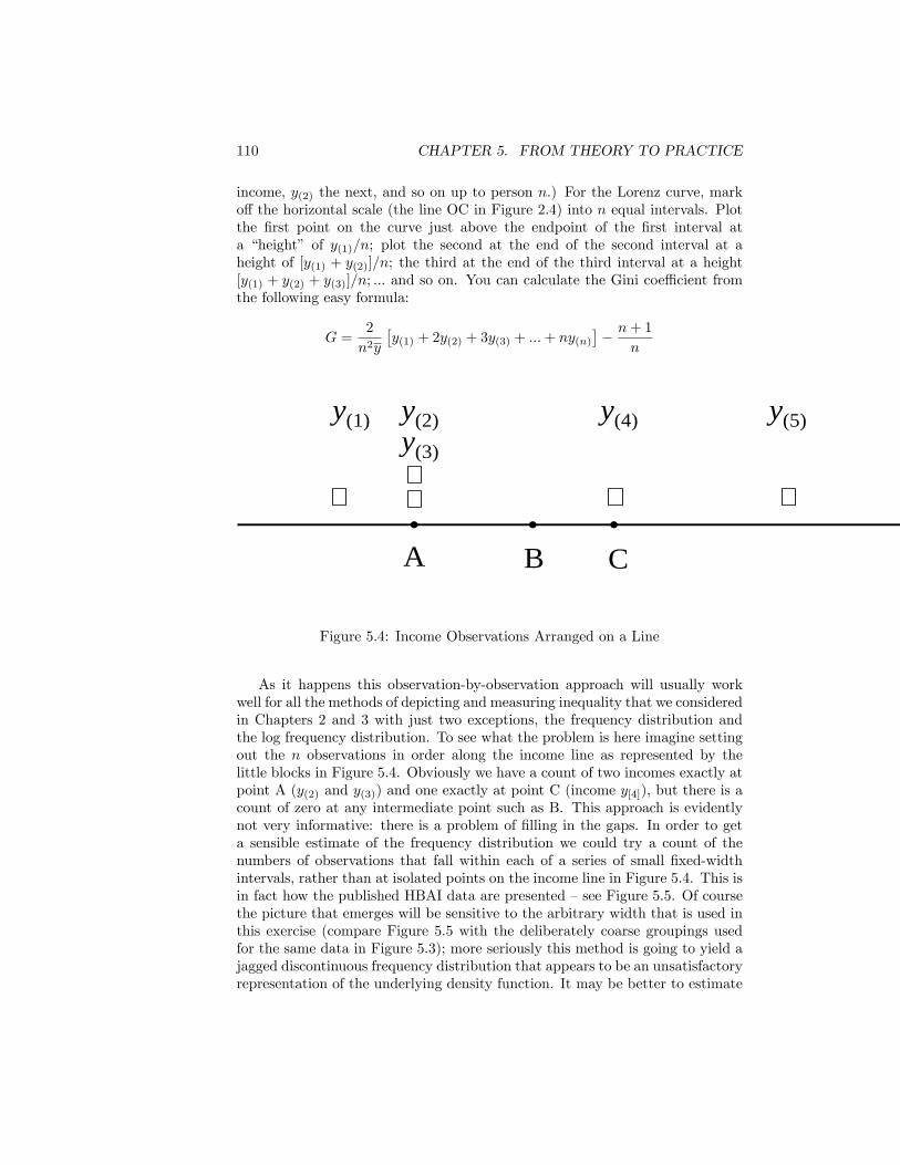
110 CHAPTER 5. FROM THEORY TO PRACTICE
income, y(2) the next, and so on up to person n.) For the Lorenz curve, marko¤ the horizontal scale (the line OC in Figure 2.4) into n equal intervals. Plotthe �rst point on the curve just above the endpoint of the �rst interval ata �height� of y(1)=n; plot the second at the end of the second interval at aheight of [y(1) + y(2)]=n; the third at the end of the third interval at a height[y(1) + y(2) + y(3)]=n; ::: and so on. You can calculate the Gini coe¢ cient fromthe following easy formula:
G =2
n2y
�y(1) + 2y(2) + 3y(3) + :::+ ny(n)
�� n+ 1
n
y(1)
A B Cy
y(2)y(3)
y(4) y(5)
• ••
Figure 5.4: Income Observations Arranged on a Line
As it happens this observation-by-observation approach will usually workwell for all the methods of depicting and measuring inequality that we consideredin Chapters 2 and 3 with just two exceptions, the frequency distribution andthe log frequency distribution. To see what the problem is here imagine settingout the n observations in order along the income line as represented by thelittle blocks in Figure 5.4. Obviously we have a count of two incomes exactly atpoint A (y(2) and y(3)) and one exactly at point C (income y[4]), but there is acount of zero at any intermediate point such as B. This approach is evidentlynot very informative: there is a problem of �lling in the gaps. In order to geta sensible estimate of the frequency distribution we could try a count of thenumbers of observations that fall within each of a series of small �xed-widthintervals, rather than at isolated points on the income line in Figure 5.4. This isin fact how the published HBAI data are presented �see Figure 5.5. Of coursethe picture that emerges will be sensitive to the arbitrary width that is used inthis exercise (compare Figure 5.5 with the deliberately coarse groupings usedfor the same data in Figure 5.3); more seriously this method is going to yield ajagged discontinuous frequency distribution that appears to be an unsatisfactoryrepresentation of the underlying density function. It may be better to estimate
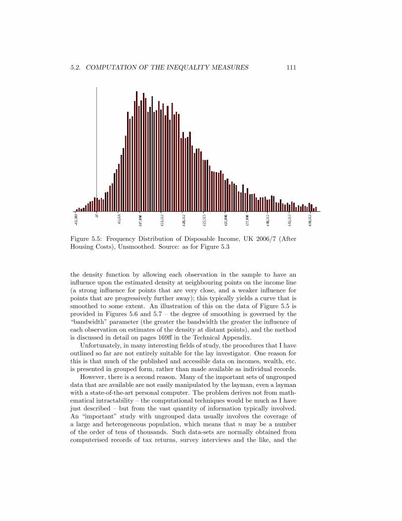
5.2. COMPUTATION OF THE INEQUALITY MEASURES 111
Figure 5.5: Frequency Distribution of Disposable Income, UK 2006/7 (AfterHousing Costs), Unsmoothed. Source: as for Figure 5.3
the density function by allowing each observation in the sample to have anin�uence upon the estimated density at neighbouring points on the income line(a strong in�uence for points that are very close, and a weaker in�uence forpoints that are progressively further away); this typically yields a curve that issmoothed to some extent. An illustration of this on the data of Figure 5.5 isprovided in Figures 5.6 and 5.7 �the degree of smoothing is governed by the�bandwidth�parameter (the greater the bandwidth the greater the in�uence ofeach observation on estimates of the density at distant points), and the methodis discussed in detail on pages 169¤ in the Technical Appendix.Unfortunately, in many interesting �elds of study, the procedures that I have
outlined so far are not entirely suitable for the lay investigator. One reason forthis is that much of the published and accessible data on incomes, wealth, etc.is presented in grouped form, rather than made available as individual records.However, there is a second reason. Many of the important sets of ungrouped
data that are available are not easily manipulated by the layman, even a laymanwith a state-of-the-art personal computer. The problem derives not from math-ematical intractability �the computational techniques would be much as I havejust described �but from the vast quantity of information typically involved.An �important� study with ungrouped data usually involves the coverage ofa large and heterogeneous population, which means that n may be a numberof the order of tens of thousands. Such data-sets are normally obtained fromcomputerised records of tax returns, survey interviews and the like, and the
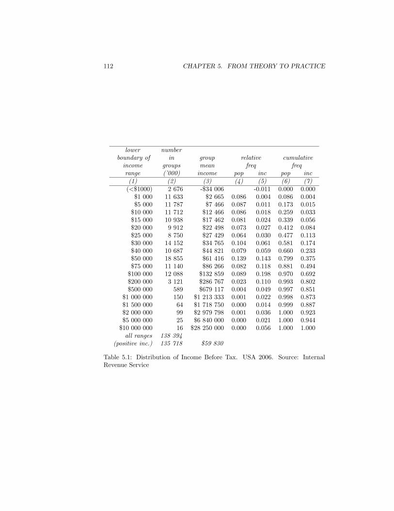
112 CHAPTER 5. FROM THEORY TO PRACTICE
lower numberboundary of in group relative cumulativeincome groups mean freq freqrange (�000) income pop inc pop inc(1) (2) (3) (4) (5) (6) (7)(<$1000) 2 676 -$34 006 -0.011 0.000 0.000$1 000 11 633 $2 665 0.086 0.004 0.086 0.004$5 000 11 787 $7 466 0.087 0.011 0.173 0.015$10 000 11 712 $12 466 0.086 0.018 0.259 0.033$15 000 10 938 $17 462 0.081 0.024 0.339 0.056$20 000 9 912 $22 498 0.073 0.027 0.412 0.084$25 000 8 750 $27 429 0.064 0.030 0.477 0.113$30 000 14 152 $34 765 0.104 0.061 0.581 0.174$40 000 10 687 $44 821 0.079 0.059 0.660 0.233$50 000 18 855 $61 416 0.139 0.143 0.799 0.375$75 000 11 140 $86 266 0.082 0.118 0.881 0.494$100 000 12 088 $132 859 0.089 0.198 0.970 0.692$200 000 3 121 $286 767 0.023 0.110 0.993 0.802$500 000 589 $679 117 0.004 0.049 0.997 0.851
$1 000 000 150 $1 213 333 0.001 0.022 0.998 0.873$1 500 000 64 $1 718 750 0.000 0.014 0.999 0.887$2 000 000 99 $2 979 798 0.001 0.036 1.000 0.923$5 000 000 25 $6 840 000 0.000 0.021 1.000 0.944$10 000 000 16 $28 250 000 0.000 0.056 1.000 1.000all ranges 138 394
(positive inc.) 135 718 $59 830
Table 5.1: Distribution of Income Before Tax. USA 2006. Source: InternalRevenue Service
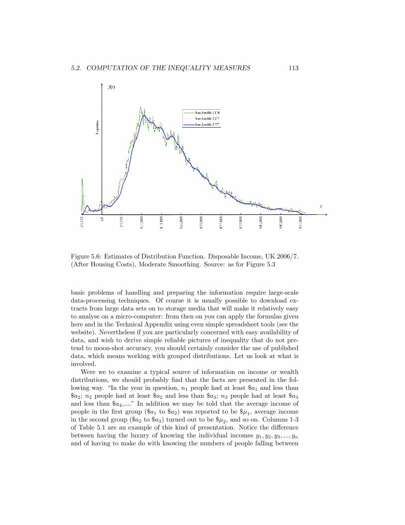
5.2. COMPUTATION OF THE INEQUALITY MEASURES 113
Figure 5.6: Estimates of Distribution Function. Disposable Income, UK 2006/7.(After Housing Costs), Moderate Smoothing. Source: as for Figure 5.3
basic problems of handling and preparing the information require large-scaledata-processing techniques. Of course it is usually possible to download ex-tracts from large data sets on to storage media that will make it relatively easyto analyse on a micro-computer: from then on you can apply the formulas givenhere and in the Technical Appendix using even simple spreadsheet tools (see thewebsite). Nevertheless if you are particularly concerned with easy availability ofdata, and wish to derive simple reliable pictures of inequality that do not pre-tend to moon-shot accuracy, you should certainly consider the use of publisheddata, which means working with grouped distributions. Let us look at what isinvolved.Were we to examine a typical source of information on income or wealth
distributions, we should probably �nd that the facts are presented in the fol-lowing way. �In the year in question, n1 people had at least $a1 and less than$a2; n2 people had at least $a2 and less than $a3; n3 people had at least $a3and less than $a4,....� In addition we may be told that the average income ofpeople in the �rst group ($a1 to $a2) was reported to be $�1, average incomein the second group ($a2 to $a3) turned out to be $�2, and so on. Columns 1-3of Table 5.1 are an example of this kind of presentation. Notice the di¤erencebetween having the luxury of knowing the individual incomes y1; y2; y3; :::; ynand of having to make do with knowing the numbers of people falling between

114 CHAPTER 5. FROM THEORY TO PRACTICE
Figure 5.7: Estimates of Distribution Function. Disposable Income, UK 2006/7.(After Housing Costs), High Smoothing. Source: as for Figure 5.3
the arbitrary income-class boundaries a1; a2; a3; ::: which have been set by thecompilers of the o¢ cial statistics.Suppose that these compilers of statistics have chopped up the income range
into a total of k intervals:
(a1; a2) (a2; a3) (a3; a4) ::: (ak; ak+1):
If we assume for the moment that a1 = 0 and ak+1 = 1, then we have indeedneatly subdivided our entire theoretical range, zero to in�nity (these assump-tions will not do in practice as we shall soon see). Accordingly, the inequalitymeasure in basic form may be modi�ed to:Z a2
a1
h(y)f(y)dy +
Z a3
a2
h(y)f(y)dy + :::+
Z ak+1
ak
h(y)f(y)dy
which can be written more simply:
kXi=1
�Z ai+1
ai
h(y)f(y)dy
�:
It may be worth repeating that this is exactly the same mathematical formulaas the �basic form�given above, the only notational di¤erence being that the
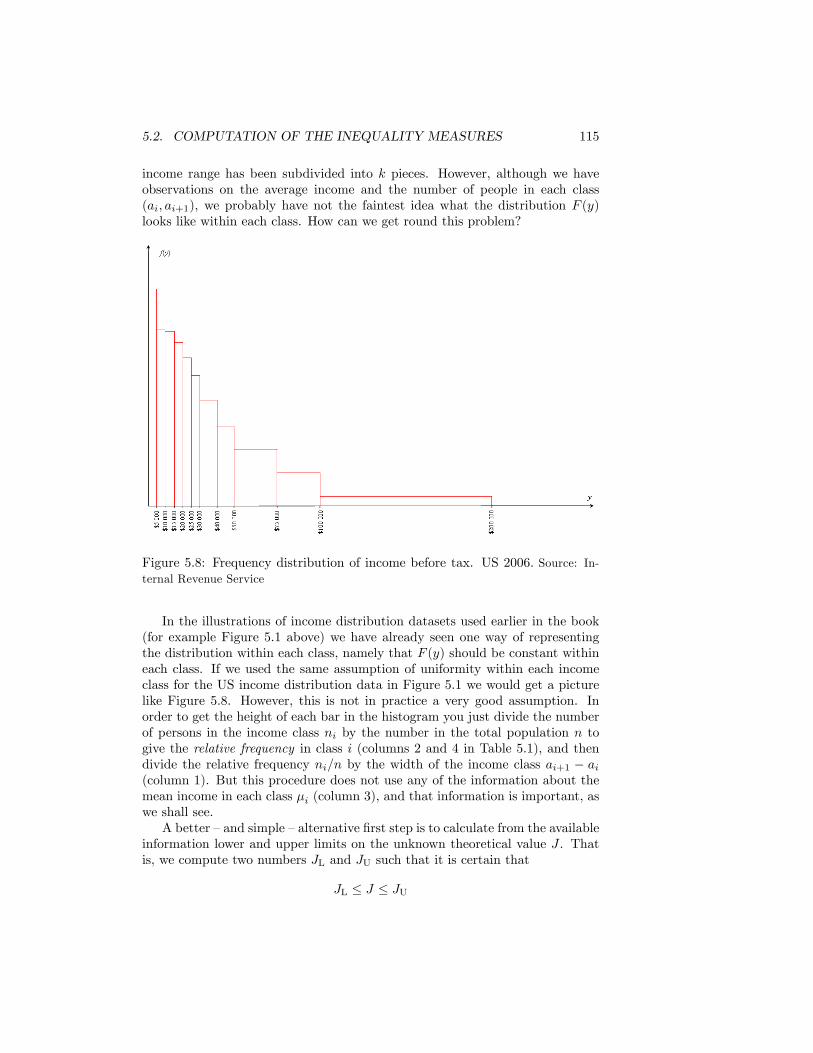
5.2. COMPUTATION OF THE INEQUALITY MEASURES 115
income range has been subdivided into k pieces. However, although we haveobservations on the average income and the number of people in each class(ai; ai+1), we probably have not the faintest idea what the distribution F (y)looks like within each class. How can we get round this problem?
Figure 5.8: Frequency distribution of income before tax. US 2006. Source: In-ternal Revenue Service
In the illustrations of income distribution datasets used earlier in the book(for example Figure 5.1 above) we have already seen one way of representingthe distribution within each class, namely that F (y) should be constant withineach class. If we used the same assumption of uniformity within each incomeclass for the US income distribution data in Figure 5.1 we would get a picturelike Figure 5.8. However, this is not in practice a very good assumption. Inorder to get the height of each bar in the histogram you just divide the numberof persons in the income class ni by the number in the total population n togive the relative frequency in class i (columns 2 and 4 in Table 5.1), and thendivide the relative frequency ni=n by the width of the income class ai+1 � ai(column 1). But this procedure does not use any of the information about themean income in each class �i (column 3), and that information is important, aswe shall see.A better �and simple �alternative �rst step is to calculate from the available
information lower and upper limits on the unknown theoretical value J . Thatis, we compute two numbers JL and JU such that it is certain that
JL � J � JU
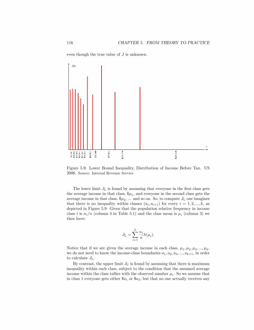
116 CHAPTER 5. FROM THEORY TO PRACTICE
even though the true value of J is unknown.
Figure 5.9: Lower Bound Inequality, Distribution of Income Before Tax. US2006. Source: Internal Revenue Service
The lower limit JL is found by assuming that everyone in the �rst class getsthe average income in that class, $�1, and everyone in the second class gets theaverage income in that class, $�2, ... and so on. So, to compute JL one imaginesthat there is no inequality within classes (ai; ai+1) for every i = 1; 2; :::; k, asdepicted in Figure 5.9. Given that the population relative frequency in incomeclass i is ni=n (column 4 in Table 5.1) and the class mean is �i (column 3) wethen have:
JL =kXi=1
ninh(�i):
Notice that if we are given the average income in each class, �1; �2; �3; :::; �k,we do not need to know the income-class boundaries a1; a2; a3; :::; ak+1, in orderto calculate JL.By contrast, the upper limit JU is found by assuming that there is maximum
inequality within each class, subject to the condition that the assumed averageincome within the class tallies with the observed number �i. So we assume thatin class 1 everyone gets either $a1 or $a2, but that no one actually receives any
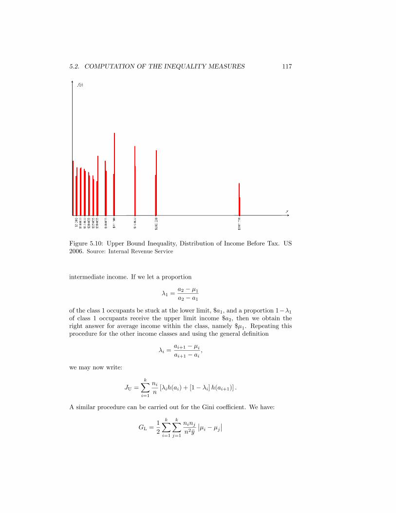
5.2. COMPUTATION OF THE INEQUALITY MEASURES 117
Figure 5.10: Upper Bound Inequality, Distribution of Income Before Tax. US2006. Source: Internal Revenue Service
intermediate income. If we let a proportion
�1 =a2 � �1a2 � a1
of the class 1 occupants be stuck at the lower limit, $a1, and a proportion 1��1of class 1 occupants receive the upper limit income $a2, then we obtain theright answer for average income within the class, namely $�1. Repeating thisprocedure for the other income classes and using the general de�nition
�i =ai+1 � �iai+1 � ai
;
we may now write:
JU =
kXi=1
nin[�ih(ai) + [1� �i]h(ai+1)] :
A similar procedure can be carried out for the Gini coe¢ cient. We have:
GL =1
2
kXi=1
kXj=1
ninjn2�y
���i � �j��
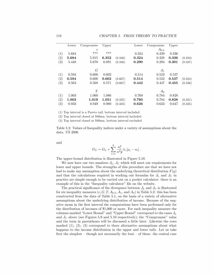
118 CHAPTER 5. FROM THEORY TO PRACTICE
Lower Compromise Upper Lower Compromise Upperc A0:5
(1) 5.684 *** *** 0.324 0.329 0.336(2) 5.684 5.915 6.352 (0.346) 0.324 0.328 0.336 (0.334)(3) 5.448 5.670 6.091 (0.346) 0.290 0.294 0.301 (0.337)
G A1(1) 0.594 0.600 0.602 0.514 0.523 0.537(2) 0.594 0.600 0.602 (0.667) 0.514 0.522 0.537 (0.324)(3) 0.563 0.568 0.571 (0.667) 0.442 0.447 0.455 (0.336)
T A2(1) 1.003 1.060 1.086 0.760 0.784 0.828(2) 1.003 1.019 1.051 (0.335) 0.760 0.784 0.828 (0.351)(3) 0.933 0.949 0.980 (0.335) 0.626 0.633 0.647 (0.335)
(1) Top interval is a Pareto tail, bottom interval included(2) Top interval closed at $40mn, bottom interval included(3) Top interval closed at $40mn, bottom interval excluded
Table 5.2: Values of Inequality indices under a variety of assumptions about thedata. US 2006
and
GU = GL +kXi=1
n2in2�y
�i [�i � ai] :
The upper-bound distribution is illustrated in Figure 5.10.We now have our two numbers JL, JU which will meet our requirements for
lower and upper bounds. The strengths of this procedure are that we have nothad to make any assumption about the underlying theoretical distribution F (y)and that the calculations required in working out formulas for JL and JU inpractice are simple enough to be carried out on a pocket calculator: there is anexample of this in the �Inequality calculator��le on the website.The practical signi�cance of the divergence between JL and JU is illustrated
for six inequality measures (c;G; T;A0:5; A1, and A2) in Table 5.2: this has beenconstructed from the data of Table 5.1, on the basis of a variety of alternativeassumptions about the underlying distribution of income. Because of the neg-ative mean in the �rst interval the computations have been performed only forthe distribution of incomes of $1,000 or more. For each inequality measure thecolumns marked �Lower Bound�and �Upper Bound�correspond to the cases JLand JU above (see Figures 5.9 and 5.10 respectively); the �Compromise�valueand the term in parentheses will be discussed a little later. Likewise the rowsmarked (1), (2), (3) correspond to three alternative assumptions about whathappens to the income distribution in the upper and lower tails. Let us take�rst the simplest �though not necessarily the best �of these: the central case
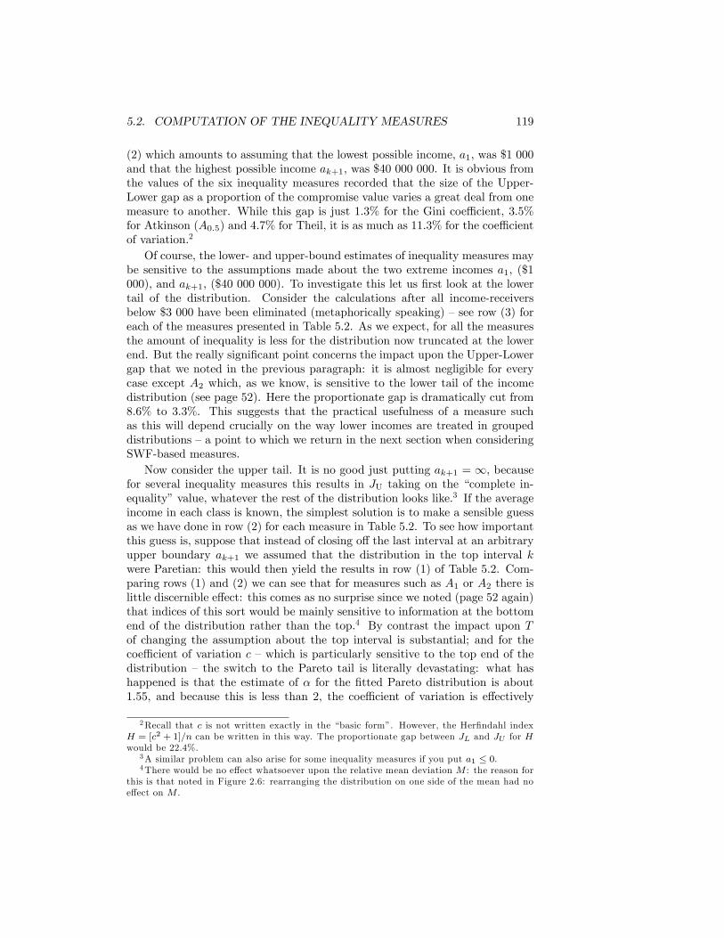
5.2. COMPUTATION OF THE INEQUALITY MEASURES 119
(2) which amounts to assuming that the lowest possible income, a1, was $1 000and that the highest possible income ak+1, was $40 000 000. It is obvious fromthe values of the six inequality measures recorded that the size of the Upper-Lower gap as a proportion of the compromise value varies a great deal from onemeasure to another. While this gap is just 1.3% for the Gini coe¢ cient, 3.5%for Atkinson (A0:5) and 4.7% for Theil, it is as much as 11.3% for the coe¢ cientof variation.2
Of course, the lower- and upper-bound estimates of inequality measures maybe sensitive to the assumptions made about the two extreme incomes a1, ($1000), and ak+1, ($40 000 000). To investigate this let us �rst look at the lowertail of the distribution. Consider the calculations after all income-receiversbelow $3 000 have been eliminated (metaphorically speaking) �see row (3) foreach of the measures presented in Table 5.2. As we expect, for all the measuresthe amount of inequality is less for the distribution now truncated at the lowerend. But the really signi�cant point concerns the impact upon the Upper-Lowergap that we noted in the previous paragraph: it is almost negligible for everycase except A2 which, as we know, is sensitive to the lower tail of the incomedistribution (see page 52). Here the proportionate gap is dramatically cut from8.6% to 3.3%. This suggests that the practical usefulness of a measure suchas this will depend crucially on the way lower incomes are treated in groupeddistributions �a point to which we return in the next section when consideringSWF-based measures.Now consider the upper tail. It is no good just putting ak+1 = 1, because
for several inequality measures this results in JU taking on the �complete in-equality�value, whatever the rest of the distribution looks like.3 If the averageincome in each class is known, the simplest solution is to make a sensible guessas we have done in row (2) for each measure in Table 5.2. To see how importantthis guess is, suppose that instead of closing o¤ the last interval at an arbitraryupper boundary ak+1 we assumed that the distribution in the top interval kwere Paretian: this would then yield the results in row (1) of Table 5.2. Com-paring rows (1) and (2) we can see that for measures such as A1 or A2 there islittle discernible e¤ect: this comes as no surprise since we noted (page 52 again)that indices of this sort would be mainly sensitive to information at the bottomend of the distribution rather than the top.4 By contrast the impact upon Tof changing the assumption about the top interval is substantial; and for thecoe¢ cient of variation c �which is particularly sensitive to the top end of thedistribution � the switch to the Pareto tail is literally devastating: what hashappened is that the estimate of � for the �tted Pareto distribution is about1.55, and because this is less than 2, the coe¢ cient of variation is e¤ectively
2Recall that c is not written exactly in the �basic form�. However, the Her�ndahl indexH = [c2 + 1]=n can be written in this way. The proportionate gap between JL and JU for Hwould be 22.4%.
3A similar problem can also arise for some inequality measures if you put a1 � 0.4There would be no e¤ect whatsoever upon the relative mean deviation M : the reason for
this is that noted in Figure 2.6: rearranging the distribution on one side of the mean had noe¤ect on M .
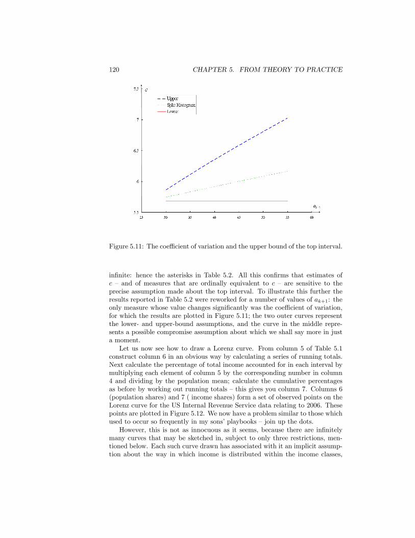
120 CHAPTER 5. FROM THEORY TO PRACTICE
Figure 5.11: The coe¢ cient of variation and the upper bound of the top interval.
in�nite: hence the asterisks in Table 5.2. All this con�rms that estimates ofc � and of measures that are ordinally equivalent to c � are sensitive to theprecise assumption made about the top interval. To illustrate this further theresults reported in Table 5.2 were reworked for a number of values of ak+1: theonly measure whose value changes signi�cantly was the coe¢ cient of variation,for which the results are plotted in Figure 5.11; the two outer curves representthe lower- and upper-bound assumptions, and the curve in the middle repre-sents a possible compromise assumption about which we shall say more in justa moment.Let us now see how to draw a Lorenz curve. From column 5 of Table 5.1
construct column 6 in an obvious way by calculating a series of running totals.Next calculate the percentage of total income accounted for in each interval bymultiplying each element of column 5 by the corresponding number in column4 and dividing by the population mean; calculate the cumulative percentagesas before by working out running totals �this gives you column 7. Columns 6(population shares) and 7 ( income shares) form a set of observed points on theLorenz curve for the US Internal Revenue Service data relating to 2006. Thesepoints are plotted in Figure 5.12. We now have a problem similar to those whichused to occur so frequently in my sons�playbooks �join up the dots.However, this is not as innocuous as it seems, because there are in�nitely
many curves that may be sketched in, subject to only three restrictions, men-tioned below. Each such curve drawn has associated with it an implicit assump-tion about the way in which income is distributed within the income classes,
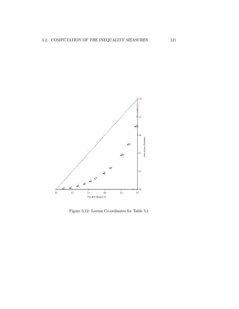
5.2. COMPUTATION OF THE INEQUALITY MEASURES 121
Figure 5.12: Lorenz Co-ordinates for Table 5.1
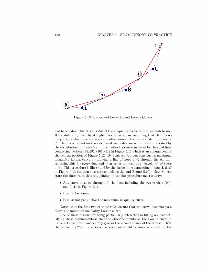
122 CHAPTER 5. FROM THEORY TO PRACTICE
Figure 5.13: Upper and Lower Bound Lorenz Curves
and hence about the �true�value of the inequality measure that we wish to use.If the dots are joined by straight lines, then we are assuming that there is noinequality within income classes �in other words, this corresponds to the use ofJL, the lower bound on the calculated inequality measure, (also illustrated bythe distribution in Figure 5.9). This method is shown in detail by the solid linesconnecting vertices (8), (9), (10), (11) in Figure 5.13 which is an enlargement ofthe central portion of Figure 5.12. By contrast you can construct a maximuminequality Lorenz curve by drawing a line of slope ai=�y through the ith dot,repeating this for every dot, and then using the resulting �envelope� of theselines. This procedure is illustrated by the dashed line connecting points A;B;Cin Figure 5.13 (in turn this corresponds to JU and Figure 5.10). Now we canstate the three rules that any joining-up-the-dot procedure must satisfy:
� Any curve must go through all the dots, including the two vertices (0,0)and (1,1) in Figure 5.12.
� It must be convex.
� It must not pass below the maximum inequality curve.
Notice that the �rst two of these rules ensure that the curve does not passabove the minimum-inequality Lorenz curve.One of these reasons for being particularly interested in �tting a curve sat-
isfying these requirements is that the observed points on the Lorenz curve inTable 5.1 (columns 6 and 7) only give us the income shares of the bottom 8.6%,the bottom 17.2%,... and so on, whereas we would be more interested in the
5.2. COMPUTATION OF THE INEQUALITY MEASURES 123
shares of, say, the bottom 10%, the bottom 20%, and to get these we must inter-polate on a curve between the points. Presumably the interpolation should bedone using neither the extreme upper- or lower-bound assumptions but ratheraccording to some �compromise� Lorenz curve. One suggestion for this com-promise method is to use the basic Pareto interpolation formula (A.3) (given onpage 154 in the Technical Appendix), which is much less fearsome than it looks,because you do not have to compute the parameters �, along the way. All youneed are the population and income shares. Unfortunately this simplicity is alsoits weakness. Because the formula does not use information about the �is theresulting curve may violate the third condition cited above (the same problemwould arise if we used a Lorenz curve based on the simple histogram densityfunction illustrated in Figure 5.14).An alternative method �which may be implemented so that all three con-
ditions are satis�ed �is to �t a theoretical frequency distribution within eachinterval in Figure 5.14), and work out the Lorenz curve from that. What fre-quency distribution? In fact it does not matter very much what type is used:all the standard �compromise� interpolation methods5 produce inequality es-timates that are remarkably similar. These methods (which are more easilyexplained using the associated density function) include:
� a �split histogram�density function in each interval. This is illustratedin Figure 5.14: contrasting this with Figure 5.8 you will note that in eachinterval there are two horizontal �steps� rather than a single step in thecase of the regular histogram; this simple device enables one to use all theinformation about the interval and is the procedure that was used for the�compromise�column in Table 5.2;
� a separate straight line density function �tted to each interval;6
� loglinear interpolation in each interval. This is in e¤ect a separate Paretodistribution �tted to each interval (ai; ai+1), using all the available infor-mation;
� a quadratic interpolation in each interval.
The details of all of these �and of how to derive the associated Lorenz curvefor each one �are given in the Technical Appendix.It is reasonably straightforward to use any of these methods to compute a
compromise value for an inequality measure. But if you do not need moon-shotaccuracy, then there is another delightfully simple method of deriving a compro-mise inequality estimate. The clue to this is in fact illustrated by the columnsin parentheses in Table 5.2: this column gives, for each inequality measure, therelative position of the compromise estimate in the interval (JL,JU) (if the com-promise estimate were exactly halfway between the lower and the upper bound,
5A minimal requirement is that the underlying density function be well-de�ned and piece-wise continuous (Cowell and Mehta 1982).
6A straight line density function implies that the corresponding Lorenz curve is a quadratic.
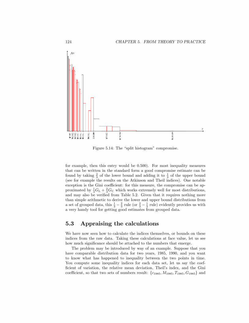
124 CHAPTER 5. FROM THEORY TO PRACTICE
Figure 5.14: The �split histogram�compromise.
for example, then this entry would be 0:500). For most inequality measuresthat can be written in the standard form a good compromise estimate can befound by taking 2
3 of the lower bound and adding it to13 of the upper bound
(see for example the results on the Atkinson and Theil indices). One notableexception is the Gini coe¢ cient: for this measure, the compromise can be ap-proximated by 1
3GL +23GU which works extremely well for most distributions,
and may also be veri�ed from Table 5.2. Given that it requires nothing morethan simple arithmetic to derive the lower and upper bound distributions froma set of grouped data, this 13 �
23 rule (or
23 �
13 rule) evidently provides us with
a very handy tool for getting good estimates from grouped data.
5.3 Appraising the calculations
We have now seen how to calculate the indices themselves, or bounds on theseindices from the raw data. Taking these calculations at face value, let us seehow much signi�cance should be attached to the numbers that emerge.The problem may be introduced by way of an example. Suppose that you
have comparable distribution data for two years, 1985, 1990, and you wantto know what has happened to inequality between the two points in time.You compute some inequality indices for each data set, let us say the coef-�cient of variation, the relative mean deviation, Theil�s index, and the Ginicoe¢ cient, so that two sets of numbers result: {c1985;M1985; T1985; G1985} and
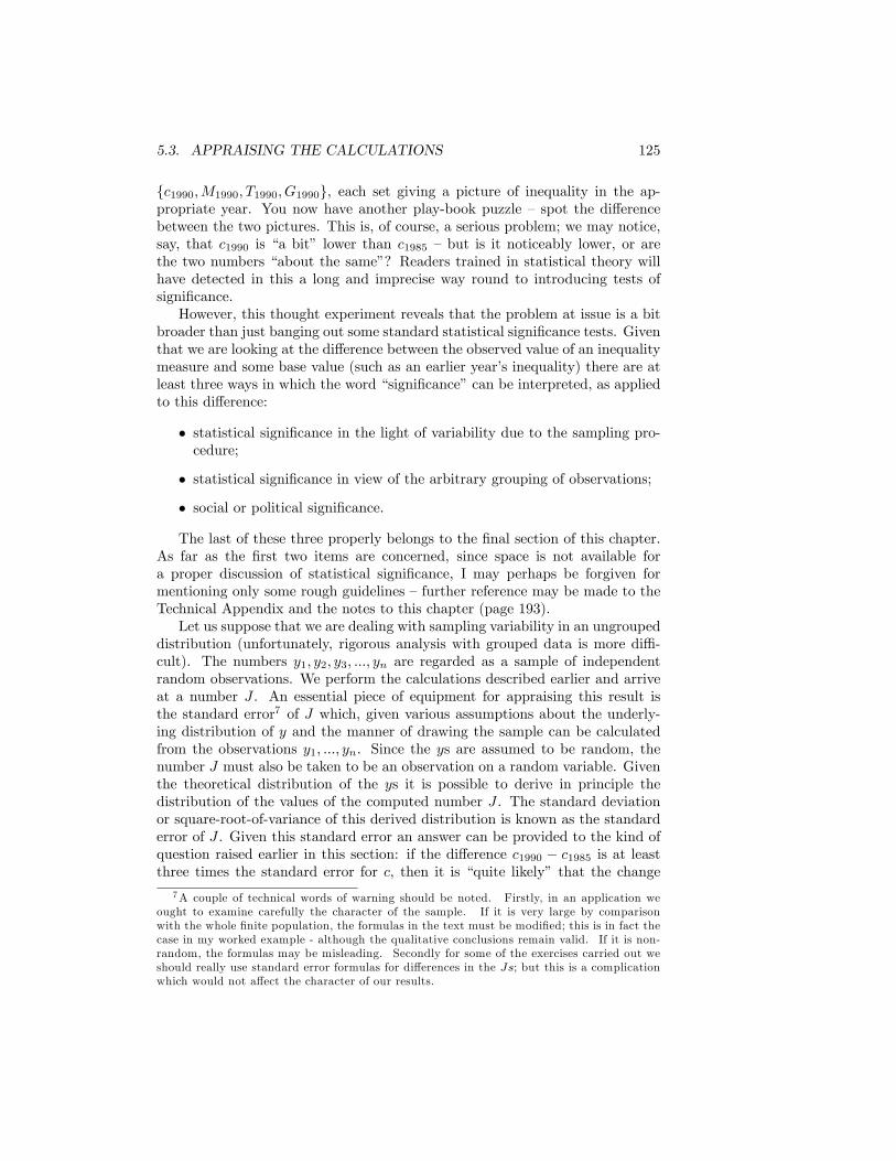
5.3. APPRAISING THE CALCULATIONS 125
{c1990;M1990; T1990; G1990}, each set giving a picture of inequality in the ap-propriate year. You now have another play-book puzzle � spot the di¤erencebetween the two pictures. This is, of course, a serious problem; we may notice,say, that c1990 is �a bit� lower than c1985 �but is it noticeably lower, or arethe two numbers �about the same�? Readers trained in statistical theory willhave detected in this a long and imprecise way round to introducing tests ofsigni�cance.However, this thought experiment reveals that the problem at issue is a bit
broader than just banging out some standard statistical signi�cance tests. Giventhat we are looking at the di¤erence between the observed value of an inequalitymeasure and some base value (such as an earlier year�s inequality) there are atleast three ways in which the word �signi�cance�can be interpreted, as appliedto this di¤erence:
� statistical signi�cance in the light of variability due to the sampling pro-cedure;
� statistical signi�cance in view of the arbitrary grouping of observations;
� social or political signi�cance.
The last of these three properly belongs to the �nal section of this chapter.As far as the �rst two items are concerned, since space is not available fora proper discussion of statistical signi�cance, I may perhaps be forgiven formentioning only some rough guidelines �further reference may be made to theTechnical Appendix and the notes to this chapter (page 193).Let us suppose that we are dealing with sampling variability in an ungrouped
distribution (unfortunately, rigorous analysis with grouped data is more di¢ -cult). The numbers y1; y2; y3; :::; yn are regarded as a sample of independentrandom observations. We perform the calculations described earlier and arriveat a number J . An essential piece of equipment for appraising this result isthe standard error7 of J which, given various assumptions about the underly-ing distribution of y and the manner of drawing the sample can be calculatedfrom the observations y1; :::; yn. Since the ys are assumed to be random, thenumber J must also be taken to be an observation on a random variable. Giventhe theoretical distribution of the ys it is possible to derive in principle thedistribution of the values of the computed number J . The standard deviationor square-root-of-variance of this derived distribution is known as the standarderror of J . Given this standard error an answer can be provided to the kind ofquestion raised earlier in this section: if the di¤erence c1990 � c1985 is at leastthree times the standard error for c, then it is �quite likely� that the change
7A couple of technical words of warning should be noted. Firstly, in an application weought to examine carefully the character of the sample. If it is very large by comparisonwith the whole �nite population, the formulas in the text must be modi�ed; this is in fact thecase in my worked example - although the qualitative conclusions remain valid. If it is non-random, the formulas may be misleading. Secondly for some of the exercises carried out weshould really use standard error formulas for di¤erences in the Js; but this is a complicationwhich would not a¤ect the character of our results.
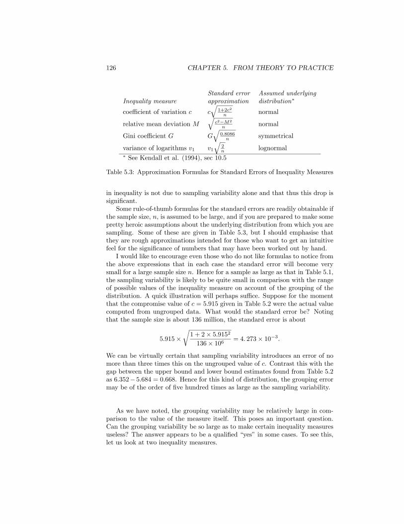
126 CHAPTER 5. FROM THEORY TO PRACTICE
Standard error Assumed underlyingInequality measure approximation distribution�
coe¢ cient of variation c cq
1+2c2
n normal
relative mean deviation Mq
c2�M2
n normal
Gini coe¢ cient G Gq
0:8086n symmetrical
variance of logarithms v1 v1
q2n lognormal
� See Kendall et al. (1994), sec 10.5
Table 5.3: Approximation Formulas for Standard Errors of Inequality Measures
in inequality is not due to sampling variability alone and that thus this drop issigni�cant.Some rule-of-thumb formulas for the standard errors are readily obtainable if
the sample size, n, is assumed to be large, and if you are prepared to make somepretty heroic assumptions about the underlying distribution from which you aresampling. Some of these are given in Table 5.3, but I should emphasise thatthey are rough approximations intended for those who want to get an intuitivefeel for the signi�cance of numbers that may have been worked out by hand.I would like to encourage even those who do not like formulas to notice from
the above expressions that in each case the standard error will become verysmall for a large sample size n. Hence for a sample as large as that in Table 5.1,the sampling variability is likely to be quite small in comparison with the rangeof possible values of the inequality measure on account of the grouping of thedistribution. A quick illustration will perhaps su¢ ce. Suppose for the momentthat the compromise value of c = 5:915 given in Table 5.2 were the actual valuecomputed from ungrouped data. What would the standard error be? Notingthat the sample size is about 136 million, the standard error is about
5:915�r1 + 2� 5:9152136� 106 = 4: 273� 10�3:
We can be virtually certain that sampling variability introduces an error of nomore than three times this on the ungrouped value of c. Contrast this with thegap between the upper bound and lower bound estimates found from Table 5.2as 6:352� 5:684 = 0:668. Hence for this kind of distribution, the grouping errormay be of the order of �ve hundred times as large as the sampling variability.
As we have noted, the grouping variability may be relatively large in com-parison to the value of the measure itself. This poses an important question.Can the grouping variability be so large as to make certain inequality measuresuseless? The answer appears to be a quali�ed �yes�in some cases. To see this,let us look at two inequality measures.

5.3. APPRAISING THE CALCULATIONS 127
Figure 5.15: Lorenz Curves �Income Before Tax. USA 1987 and 2006. Source:Internal Revenue Service
First, take the coe¢ cient of variation that we have just been discussing.From Table 5.2 we know that the value of c in 2006 lies in the range (5.684,6.352) � see the bottom row of Table 5.4. The corresponding values for of cfor some earlier years are also shown on the left-hand side of Table 5.4. Itis immediately clear that, even though the (cL; cU) gap is large in every year,inequality in 2006 was unquestionably higher than in any of the other threeyears shown.8 Figure 5.15 illustrates why this is so: it is clear to the naked eyethat the Lorenz curve for 1987 dominates that for 2006; even if we drew in theupper-bound and lower-bound Lorenz curves for each year this conclusion willnot go away. By contrast we cannot immediately say that, say, c was higher in1995 than 1987: the lower-bound, compromise, and upper-bound estimates of call grew by about 11 12 percent over the period but, in either year, the (cL; cU)gap (as a proportion of the compromise value) is over 22 percent.Next consider Atkinson�s measure A"for the same data. The lower and upper
bounds and compromise value are represented pictorially in Figure 5.16. We can
8The lower-bound and compromise values of c more than double from 2001 to 2006. HereI am making the assumption that the top interval is closed as in case (2) of Table 5.2. Hadwe assumed that the top interval had a Pareto tail (case 1) then we would have found that cwas unbounded in each of the four years �see the �inequality calculator� on the website.
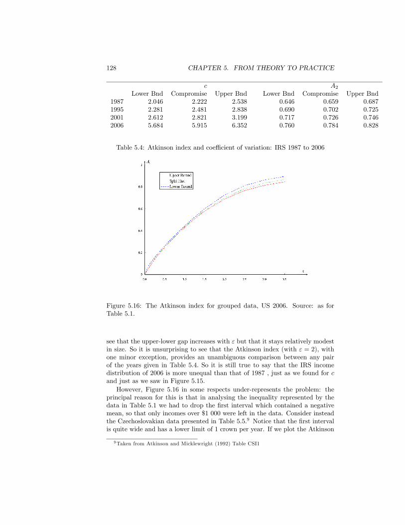
128 CHAPTER 5. FROM THEORY TO PRACTICE
c A2Lower Bnd Compromise Upper Bnd Lower Bnd Compromise Upper Bnd
1987 2.046 2.222 2.538 0.646 0.659 0.6871995 2.281 2.481 2.838 0.690 0.702 0.7252001 2.612 2.821 3.199 0.717 0.726 0.7462006 5.684 5.915 6.352 0.760 0.784 0.828
Table 5.4: Atkinson index and coe¢ cient of variation: IRS 1987 to 2006
Figure 5.16: The Atkinson index for grouped data, US 2006. Source: as forTable 5.1.
see that the upper-lower gap increases with " but that it stays relatively modestin size. So it is unsurprising to see that the Atkinson index (with " = 2), withone minor exception, provides an unambiguous comparison between any pairof the years given in Table 5.4. So it is still true to say that the IRS incomedistribution of 2006 is more unequal than that of 1987 , just as we found for cand just as we saw in Figure 5.15.However, Figure 5.16 in some respects under-represents the problem: the
principal reason for this is that in analysing the inequality represented by thedata in Table 5.1 we had to drop the �rst interval which contained a negativemean, so that only incomes over $1 000 were left in the data. Consider insteadthe Czechoslovakian data presented in Table 5.5.9 Notice that the �rst intervalis quite wide and has a lower limit of 1 crown per year. If we plot the Atkinson
9Taken from Atkinson and Micklewright (1992) Table CSI1
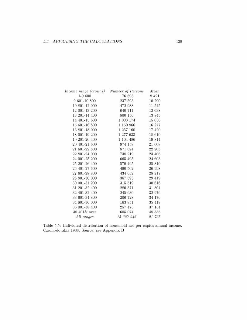
5.3. APPRAISING THE CALCULATIONS 129
Income range (crowns) Number of Persons Mean1-9 600 176 693 8 421
9 601-10 800 237 593 10 29010 801-12 000 472 988 11 54512 001-13 200 640 711 12 63813 201-14 400 800 156 13 84514 401-15 600 1 003 174 15 03615 601-16 800 1 160 966 16 27716 801-18 000 1 257 160 17 42018 001-19 200 1 277 633 18 61019 201-20 400 1 104 486 19 81420 401-21 600 974 158 21 00821 601-22 800 871 624 22 20322 801-24 000 738 219 23 40624 001-25 200 665 495 24 60325 201-26 400 579 495 25 81026 401-27 600 490 502 26 99827 601-28 800 434 652 28 21728 801-30 000 367 593 29 41930 001-31 200 315 519 30 61631 201-32 400 280 371 31 80432 401-32 400 245 630 32 97633 601-34 800 206 728 34 17634 801-36 000 163 851 35 41836 001-38 400 257 475 37 15438 401& over 605 074 48 338All ranges 15 327 946 21 735
Table 5.5: Individual distribution of household net per capita annual income.Czechoslovakia 1988. Source: see Appendix B

130 CHAPTER 5. FROM THEORY TO PRACTICE
0
0.02
0.04
0.06
0.08
0.1
0.12
0.14
0.16
0.18
0.2
0.0
0.5
1.0
1.5
2.0
2.5
3.0
3.5
4.0
upper
split histog
lower
ε
Aε
Figure 5.17: The Atkinson Index for Grouped Data: First interval deleted.Czechoslovakia 1988
index for these data and drop the �rst interval (as we did for the Americandata) it appears that inequality is quite low �see the picture in Figure 5.17 �and this picture is in fact borne out by other inequality measures as well as A".But if we attempt to take account of all the data �including the �rst interval�then the picture of Figure 5.18 emerges. Notice that not only is the upper-bound estimate of inequality seriously a¤ected for "> 1 (which we might haveguessed) but so too is the compromise value. Obviously truncating the data (ormanipulating in some other way the assumption about a1 which is causing allthe trouble) is convenient, but in one sense this is to avoid the problem, sincewe are deliberately ignoring incomes in the range where our inequality measureis designed to be particularly sensitive. The unpalatable conclusion is thatbecause of grouping error (and perhaps sampling error too) either we shall haveto discard certain sensitive measures of inequality from our toolkit on empiricalgrounds, or the distribution must provide extremely detailed information aboutlow incomes so that measures with high inequality aversion can be used, or theincome distribution �gures will have to be truncated or doctored at the lowerend in a way which may reduce their relevance in the particular area of socialenquiry.
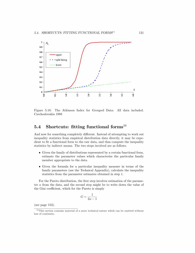
5.4. SHORTCUTS: FITTING FUNCTIONAL FORMS11 131
0
0.1
0.2
0.3
0.4
0.5
0.6
0.7
0.8
0.9
10.
0
0.5
1.0
1.5
2.0
2.5
3.0
3.5
4.0
upper
split histog
lower
ε
Aε
Figure 5.18: The Atkinson Index for Grouped Data: All data included.Czechoslovakia 1988
5.4 Shortcuts: �tting functional forms10
And now for something completely di¤erent. Instead of attempting to work outinequality statistics from empirical distribution data directly, it may be expe-dient to �t a functional form to the raw data, and thus compute the inequalitystatistics by indirect means. The two steps involved are as follows.
� Given the family of distributions represented by a certain functional form,estimate the parameter values which characterise the particular familymember appropriate to the data.
� Given the formula for a particular inequality measure in terms of thefamily parameters (see the Technical Appendix), calculate the inequalitystatistics from the parameter estimates obtained in step 1.
For the Pareto distribution, the �rst step involves estimation of the parame-ter � from the data, and the second step might be to write down the value ofthe Gini coe¢ cient, which for the Pareto is simply
G =1
2�� 1
(see page 153).
10This section contains material of a more technical nature which can be omitted withoutloss of continuity.
132 CHAPTER 5. FROM THEORY TO PRACTICE
For the lognormal distribution, the �rst step involves estimation of �2. Sincethe second step is simple once you have the formula (it usually involves merelyan ordinally equivalent transformation of one of the parameters), I shall onlyconsider in detail methods relating to the �rst step � the estimation of theparameters.Two words of warning. Up to now we have used symbols such as �y, V , etc.
to denote the theoretical mean, variance, etc., of some distribution. From nowon, these symbols will represent the computed mean, variance, etc., of the set ofobservations that we have under consideration. Although this is a little sloppy,it avoids introducing more symbols. Also, note that often there is more than onesatisfactory method of estimating a parameter value, yielding di¤erent results.Under such circumstances it is up to the user to decide on the relative meritsof the alternative methods.Let us move straightaway on to the estimation of the parameters of the
lognormal distribution for ungrouped and for grouped data.If the data are in ungrouped form �that is we have n observations, y1; y2; :::; yn
�then on the assumption that these come from a population that is lognormal,it is easy to use the so-called method of moments to calculate estimates e�, e�2for the lognormal distribution. Calculate the mean, and the Her�ndahl index(the sum of the squares of the shares �see page 58) for these n incomes:
H =
nXi=1
�yiny
�2Then we �nd: e�2 = log(nH)
e� = log(y)� 12e�2
While this is very easy, it is not as e¢ cient12 as the following method.An alternative procedure that is fairly straightforward for ungrouped data
is to derive the maximum likelihood estimates, �̂, �̂2. To do this, transform allthe observations y1; y2; :::; yn to their logarithms x1; x2; :::; xn. Then calculate:
�̂ =1
n
nXi=1
xi
�̂2 =1
n
nXi=1
[xi � �̂]2
It is evident that �̂ is simply log(y�) �the logarithm of the geometric mean,and that �̂2 is v1, the variance of the logarithms de�ned relative to y�.In the case of grouped data, maximum likelihood methods are available, but
they are too involved to set out here. However, the method of moments can
12The standard errors of the estimates will be larger than those for the maximum likelihoodprocedure (which is the most e¢ cient in this case).
5.4. SHORTCUTS: FITTING FUNCTIONAL FORMS13 133
be applied similarly to the way it was done in the ungrouped case, providedthat in the computation of H an appropriate correction is made to allow for thegrouping of observation.We shall go straight on now to consider the estimation of the parameters of
the Pareto distribution, once again dealing �rst with ungrouped data.For the method of moments, once again arrange the n observations y1; y2; :::; yn
in Parade order y(1); y(2); :::; y(n); (as on page 109). It can be shown that theexpected value of the lowest observation y(1), given the assumption that thesample has been drawn at random from a Pareto distribution with parameters�, is ny=[n � 1]. Work out the observed mean income y. We already know(from page 90) the expected value of this, given the Pareto assumption: it is�y=[�� 1]. We now simply equate the sample observations (y(1) and y) to theirexpected values:
y(1) =�ny
�n� 1
y =�y
�� 1Solving these two simple equations in two unknowns �, y we �nd the method-of-moments estimates for the two parameters:
e� = y � y(1)n
y � y(1)
ey = �1� 1e��y
However, this procedure is not suitable for grouped data. By contrast, theordinary least squares method for estimating � can be applied whether the dataare grouped or not. Recall the point in Chapter 4 that if y is any income level,and P is the proportion of the population with that income or more, then underthe Pareto distribution, a linear relationship exists between log(P ) and log(y),the slope of the line being �. Indeed we may write this as
p = z � �x
where p represents log(P ), x represents log(y), and z gives the intercept of thestraight line.Given a set of ungrouped observations y1; y2; :::; yn arranged say in ascending
size order, it is easy to set up the estimating equation for �. For the �rstobservation, since the entire sample has that income or more (P = 1), therelevant value of p is
p1 = log(1) = 0
For the second observation, we have
p2 = log
�1� 1
n
�
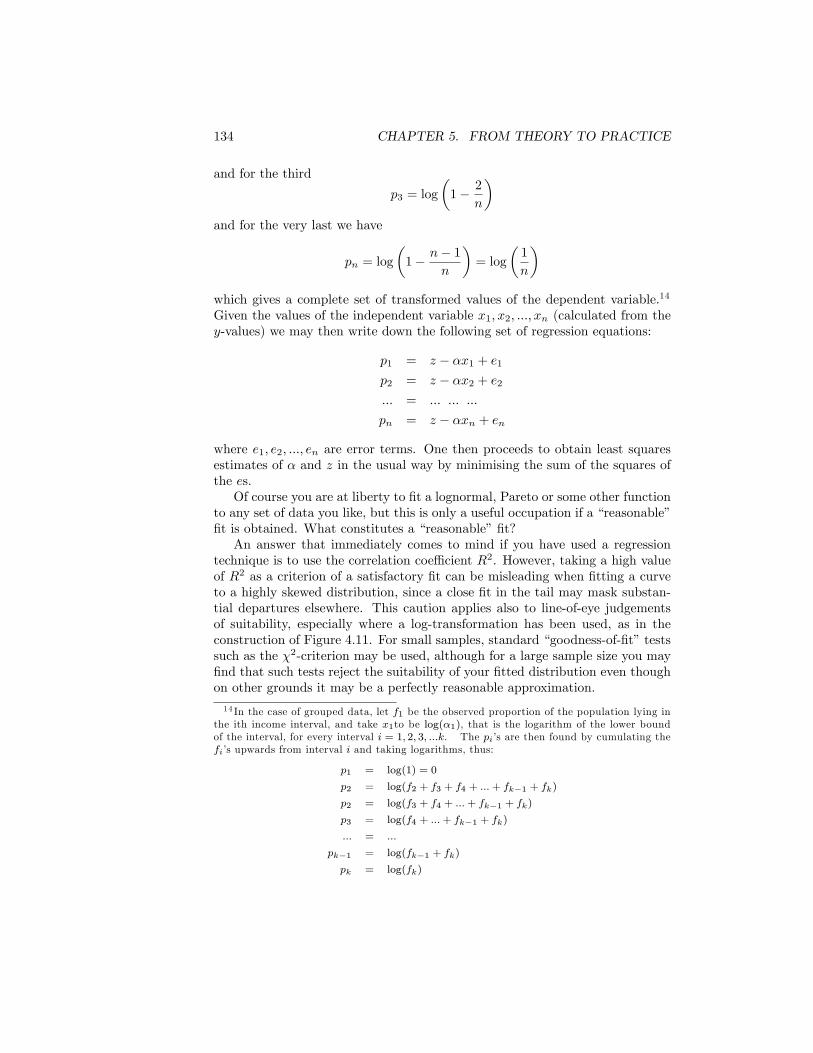
134 CHAPTER 5. FROM THEORY TO PRACTICE
and for the third
p3 = log
�1� 2
n
�and for the very last we have
pn = log
�1� n� 1
n
�= log
�1
n
�which gives a complete set of transformed values of the dependent variable.14
Given the values of the independent variable x1; x2; :::; xn (calculated from they-values) we may then write down the following set of regression equations:
p1 = z � �x1 + e1p2 = z � �x2 + e2::: = ::: ::: :::
pn = z � �xn + en
where e1; e2; :::; en are error terms. One then proceeds to obtain least squaresestimates of � and z in the usual way by minimising the sum of the squares ofthe es.Of course you are at liberty to �t a lognormal, Pareto or some other function
to any set of data you like, but this is only a useful occupation if a �reasonable��t is obtained. What constitutes a �reasonable��t?An answer that immediately comes to mind if you have used a regression
technique is to use the correlation coe¢ cient R2. However, taking a high valueof R2 as a criterion of a satisfactory �t can be misleading when �tting a curveto a highly skewed distribution, since a close �t in the tail may mask substan-tial departures elsewhere. This caution applies also to line-of-eye judgementsof suitability, especially where a log-transformation has been used, as in theconstruction of Figure 4.11. For small samples, standard �goodness-of-�t�testssuch as the �2-criterion may be used, although for a large sample size you may�nd that such tests reject the suitability of your �tted distribution even thoughon other grounds it may be a perfectly reasonable approximation.
14 In the case of grouped data, let f1 be the observed proportion of the population lying inthe ith income interval, and take x1to be log(�1), that is the logarithm of the lower boundof the interval, for every interval i = 1; 2; 3; :::k. The pi�s are then found by cumulating thefi�s upwards from interval i and taking logarithms, thus:
p1 = log(1) = 0
p2 = log(f2 + f3 + f4 + :::+ fk�1 + fk)
p2 = log(f3 + f4 + :::+ fk�1 + fk)
p3 = log(f4 + :::+ fk�1 + fk)
::: = :::
pk�1 = log(fk�1 + fk)
pk = log(fk)
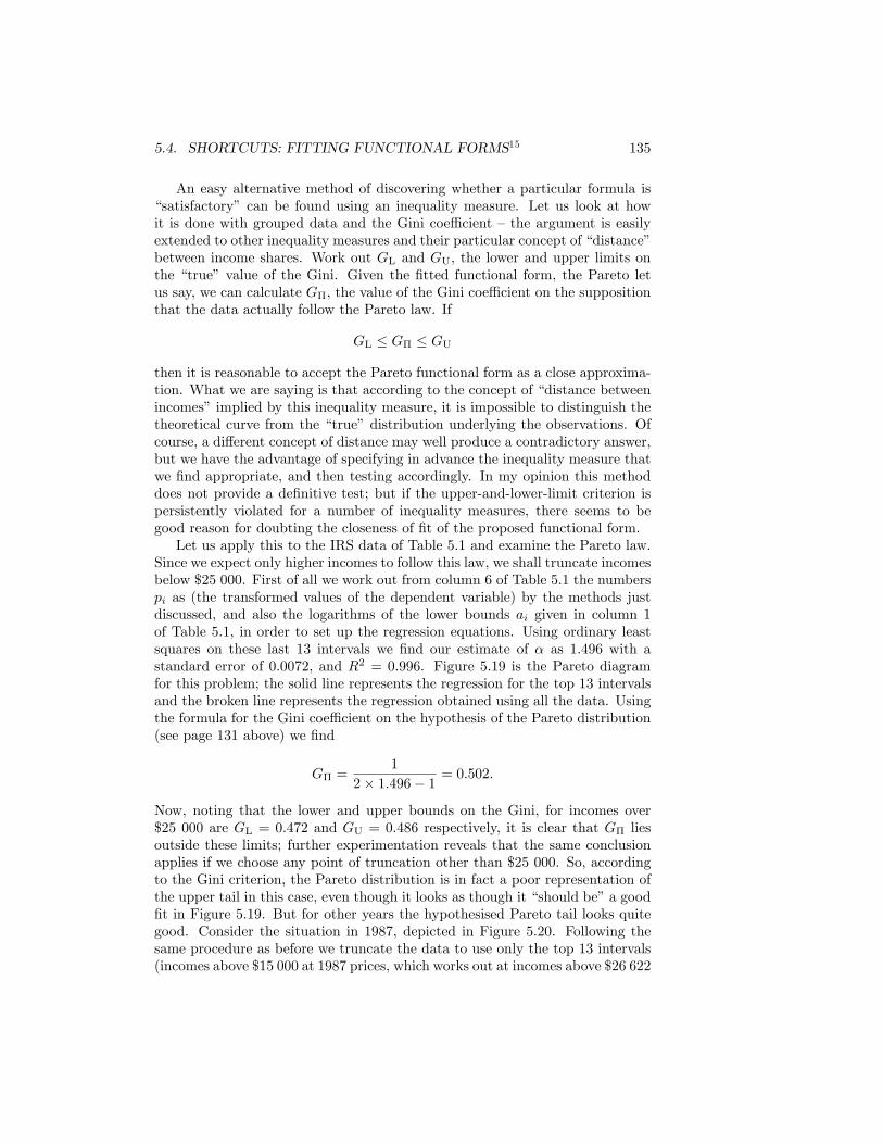
5.4. SHORTCUTS: FITTING FUNCTIONAL FORMS15 135
An easy alternative method of discovering whether a particular formula is�satisfactory� can be found using an inequality measure. Let us look at howit is done with grouped data and the Gini coe¢ cient �the argument is easilyextended to other inequality measures and their particular concept of �distance�between income shares. Work out GL and GU, the lower and upper limits onthe �true� value of the Gini. Given the �tted functional form, the Pareto letus say, we can calculate G�, the value of the Gini coe¢ cient on the suppositionthat the data actually follow the Pareto law. If
GL � G� � GU
then it is reasonable to accept the Pareto functional form as a close approxima-tion. What we are saying is that according to the concept of �distance betweenincomes�implied by this inequality measure, it is impossible to distinguish thetheoretical curve from the �true�distribution underlying the observations. Ofcourse, a di¤erent concept of distance may well produce a contradictory answer,but we have the advantage of specifying in advance the inequality measure thatwe �nd appropriate, and then testing accordingly. In my opinion this methoddoes not provide a de�nitive test; but if the upper-and-lower-limit criterion ispersistently violated for a number of inequality measures, there seems to begood reason for doubting the closeness of �t of the proposed functional form.Let us apply this to the IRS data of Table 5.1 and examine the Pareto law.
Since we expect only higher incomes to follow this law, we shall truncate incomesbelow $25 000. First of all we work out from column 6 of Table 5.1 the numberspi as (the transformed values of the dependent variable) by the methods justdiscussed, and also the logarithms of the lower bounds ai given in column 1of Table 5.1, in order to set up the regression equations. Using ordinary leastsquares on these last 13 intervals we �nd our estimate of � as 1.496 with astandard error of 0.0072, and R2 = 0:996. Figure 5.19 is the Pareto diagramfor this problem; the solid line represents the regression for the top 13 intervalsand the broken line represents the regression obtained using all the data. Usingthe formula for the Gini coe¢ cient on the hypothesis of the Pareto distribution(see page 131 above) we �nd
G� =1
2� 1:496� 1 = 0:502:
Now, noting that the lower and upper bounds on the Gini, for incomes over$25 000 are GL = 0:472 and GU = 0:486 respectively, it is clear that G� liesoutside these limits; further experimentation reveals that the same conclusionapplies if we choose any point of truncation other than $25 000. So, accordingto the Gini criterion, the Pareto distribution is in fact a poor representation ofthe upper tail in this case, even though it looks as though it �should be�a good�t in Figure 5.19. But for other years the hypothesised Pareto tail looks quitegood. Consider the situation in 1987, depicted in Figure 5.20. Following thesame procedure as before we truncate the data to use only the top 13 intervals(incomes above $15 000 at 1987 prices, which works out at incomes above $26 622
136 CHAPTER 5. FROM THEORY TO PRACTICE
Figure 5.19: Fitting the Pareto diagram for the data in Table 5.1
in 2006 prices). Now we �nd the estimated � to be 1.879 (s.e. = 0.0092, R2 =0.992) so that
G� =1
2� 1:879� 1 = 0:3625:
In this case GL = 0:3554 and GU = 0:3628 and G� lies within these bound.So the Pareto distribution certainly seems to be an acceptable �t for the top13 income classes in 1987. In passing it is interesting to see how dramaticallyinequality increased over the period 1987 to 2006 �a point which we had alreadynoted from Figure 4.12.Two points should be noted from this exercise. First, just relying on judg-
ment by eye may be unsatisfactory �the Pareto tail yielded a misleading esti-mate of the Gini coe¢ cient in 2006. Second, had we relied on the R2 criterionalone, however, we would also have been seriously led astray. If we reworkedthe 2006 calculations for all incomes above $1 000 we would still have a high R2
(0.918) but a much lower value of � (1.185); the implied value of G� = 0:616lies well above the upper bound GU = 0:602 recorded for this group of the pop-ulation in Table 5.2, thus indicating that the Pareto distribution is in practicea bad �t for all incomes above $1 000. It is easy to see what is going on inthe Pareto diagram, Figure 5.19: as we noted the solid regression line depicts
5.4. SHORTCUTS: FITTING FUNCTIONAL FORMS16 137
Figure 5.20: Fitting the Pareto diagram for IRS data in 1987 (values in 2006dollars)
the �tted Pareto distribution for $15 000 on which we based our original cal-culations; if we were to �t a straight line to all the data (the broken line), wewould still get an impressive R2 because of the predominance of the points atthe right-hand end, but it is obvious that the straight line assumption wouldnow be rather a poor one. (This is in fact characteristic of income distributiondata: Compare the results for IRS 1987 in Figure 5.20 and for the UK data inFigure 4.5.)
It seems that we have discovered three main hazards in the terrain coveredby this section.
� We should inspect the statistical properties of the estimators involved inany �tting procedure.
� We should check which parts of the distribution have had to be truncatedin order to make the �t �work.�
� We must take care over the �goodness-of-�t�criterion employed.
However, in my opinion, none of these three is as hard as the less technicalproblems which we encounter next.
138 CHAPTER 5. FROM THEORY TO PRACTICE
5.5 Interpreting the answers
Put yourself in the position of someone who is carrying out an independentstudy of inequality, or of one examining the summary results of some recentreport on the subject. To �x ideas, let us assume that it appears that inequalityhas decreased in the last �ve years. But presumably we are not going to swallowany story received from a computer print-out or a journal article straightaway.In this �nal and important puzzle of �colour the picture�, we will do well toquestion the colouring instructions which the presentation of the facts suggests.
� What cardinal representation has been used?� Has the cake shrunk?� Is the drop in inequality an optical illusion?� How do we cope with problems of non-comparability?� Is the trend toward equality large enough to matter?
INEQUALITY CHANGE: A CHECKLIST
Although the queries that you raise in the face of the evidence may be farmore penetrating than mine, I should like to mention some basic questions thatought to be posed, even if not satisfactorily resolved. In doing so I shall take asunderstood two issues that we have already laboured to some extent:
� that agreement has been reached on the de�nition of �income�and otherterms and on the choice of inequality measure(s);
� that we are satis�ed that the observed changes in inequality are �signi�-cant�in a statistical or formal sense as discussed in this chapter.
Each of these questions is of the sort that merits several journal articles inits own right. That being said, I am afraid that you will not �nd that they areasked often enough.
What cardinal representation has been used?
The retentive reader will recall from the �rst chapter that two inequality mea-sures, although ordinally equivalent (so that they always rank any list of socialstates in the same order), might not have equivalent cardinal properties, so thatpercentage changes in inequality could appear di¤erent according to the twomeasures.As examples of this, take the Her�ndahl index H and the coe¢ cient of
variation c. Since
H =c2 + 1
n
5.5. INTERPRETING THE ANSWERS 139
for the same population size H and c will always rank any pair of states in thesame order. However, the relative size of any di¤erence in inequality will beregistered di¤erently by H and by c. To see this, re-examine Table 5.1 where wenoted that the minimum and maximum values of c were 2.281 and 2.838, whichmeans that there is a di¤erence in measured inequality of about 22.5% whichis attributable to the e¤ect of grouping. If we did the same calculation for H,we would �nd that the gap appeared to be much larger, namely 46.4%. Themeasure H will always register larger proportional changes in inequality than c,as long as c lies above one (exactly the reverse is true for c less than one).What this implies more generally is that we should not be terribly impressed
by a remark such as �inequality has fallen by x% according to inequality mea-sure J� unless we are quite clear in our own minds that according to someother sensible and ordinally equivalent measure the quantitative results is notsubstantially di¤erent.17
Has the cake shrunk?
Again you may recollect that in Chapter 1 we noted that for much of the for-mal work it would be necessary to take as axiomatic the existence of a �xedtotal of income or wealth to be shared out. This axiom is implicit in the def-inition of many inequality measures so that they are insensitive to changes inmean income, and insofar as it isolates a pure distribution problem seems quitereasonable. However, presuming that society has egalitarian preferences,18 thestatement �inequality has decreased in the last �ve years�cannot by itself im-ply �society is now in a better state�unless one is quite sure that the total tobe divided has not drastically diminished also. Unless society is very averse toinequality, a mild reduction in inequality accompanied by a signi�cant drop inaverage income may well be regarded as a de�nitely retrograde change.We can formulate this readily in the case of an inequality measure that is ex-
plicitly based upon a social-welfare function: by writing down the social-welfarefunction in terms of individual incomes y1; y2; :::; yn we are specifying both aninequality ranking and a tradeo¤ between average income and an inequalityindex consistent with this ranking.19 Atkinson�s measure A" and the social-
17A technical note. It is not su¢ cient to normalise so that the minimum value of J is 0,and the maximum value 1. For, suppose J does have this property, then so does Jm where mis any positive number, and of course, J and Jm are ordinally, but not cardinally, equivalent.18This is implied in the use of any inequality measure that satis�es the weak principle of
transfers.19Actually, this requires some care. Notice that the same inequality measure can be consis-
tent with a variety of social welfare functions. For example, if we do not restrict the SWF tobe additive, the measure A" could have been derived from any SWF of the form:
� (�y)
nXi=1
y1��i � 11� �
which means that virtually any trade-o¤ between equality and income can be obtained, de-pending on the speci�cation of �. Pre-specifying the SWF removes this ambiguity, for exam-ple, if we insist on the additivity assumption for the SWF then �=constant, and there is theunique trade-o¤ between equality and mean income.
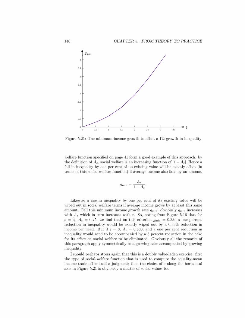
140 CHAPTER 5. FROM THEORY TO PRACTICE
ε0 0.5 1 1.5 2 2.5 3 3.5
0
0.5
1
1.5
2
2.5
3
3.5
4
gmin
Figure 5.21: The minimum income growth to o¤set a 1% growth in inequality
welfare function speci�ed on page 41 form a good example of this approach: bythe de�nition of A", social welfare is an increasing function of [1�A"]: Hence afall in inequality by one per cent of its existing value will be exactly o¤set (interms of this social-welfare function) if average income also falls by an amount
gmin =A"
1�A":
Likewise a rise in inequality by one per cent of its existing value will bewiped out in social welfare terms if average income grows by at least this sameamount. Call this minimum income growth rate gmin: obviously gmin increaseswith A" which in turn increases with ". So, noting from Figure 5.16 that for" = 1
2 , A" = 0:25, we �nd that on this criterion gmin = 0:33: a one percentreduction in inequality would be exactly wiped out by a 0.33% reduction inincome per head. But if " = 3, A" = 0:833, and a one per cent reduction ininequality would need to be accompanied by a 5 percent reduction in the cakefor its e¤ect on social welfare to be eliminated. Obviously all the remarks ofthis paragraph apply symmetrically to a growing cake accompanied by growinginequality.I should perhaps stress again that this is a doubly value-laden exercise: �rst
the type of social-welfare function that is used to compute the equality-meanincome trade o¤ is itself a judgment; then the choice of " along the horizontalaxis in Figure 5.21 is obviously a matter of social values too.
5.5. INTERPRETING THE ANSWERS 141
Is the drop in inequality an optical illusion?
Unfortunately this may very well be so if we have not taken carefully intoconsideration demographic, social and occupational shifts during the period.Some of these shifts you may want to include within the ambit of inequalityanyway, but the treatment of others is less clear. Let us follow through twoexamples.First, suppose there is higher inequality of earnings among doctors than
among dockers, that relative remuneration and inequality within occupationshave not altered over time, but that there are now relatively more dockers.Inequality in the aggregate will have decreased, although the inequality of earn-ings opportunity facing a new entrant to either occupation will have remainedunchanged. Whether or not one concludes that inequality has �really� gonedown is in large part a matter of interpretation, though my opinion is that ithas done so.However, I would not be so con�dent in the case of the second example: sup-
pose income inequality within age groups increases with the age of the group(this is very often true in fact). Now imagine that the age distribution is gradu-ally shifting in favour of the young, either because the birth rate has been rising,or because pensioners are dying earlier, but that inequality within age groupsremains unaltered. It will appear that inequality is falling, but this is due en-tirely to the demographic change. Indeed, if your chances of physical survivalare closely linked to your income, the appearance that inequality is decreas-ing can be quite misleading, sine the death rate may have been substantiallyboosted by the greater inequality among the old.There are obviously several social and economic factors which ought to be
considered in a similar way. Among these are changes in the frequency of mar-riage and divorce, shifts (possibly cyclical) of the numbers of wives, children andother part-time or temporary workers in the labour force, and price changes thata¤ect people�s real incomes in di¤erent ways depending on their position in theParade of incomes.
How do we cope with problems of non-comparability?
This question follows naturally from the last and can be approached in twoways: non-comparability of types of income, and non-comparability of groupsof income recipients. In the �rst case we may well want to examine, say, theinequality of labour earnings, of income from property and the relationship ofthese quantities to overall inequality. We evidently need to have a detailedbreakdown of the income distribution both by income type and by recipient �information that is usually hard to come by. Furthermore the mechanics of therelationship between inequality of components of income and inequality of in-come as a whole are by no means straightforward �see the Technical Appendix.In the second case, while examining the e¤ect of demographic and other
shifts, we may conclude that crudely lumping together di¤erent groups of thepopulation and thus treating them as comparable in every way is unwarranted.
142 CHAPTER 5. FROM THEORY TO PRACTICE
In order to handle this di¢ culty, it helps to have an inequality measure that canbe conveniently decomposed into a component representing inequality withingroups, and a component giving inequality between groups. It would look some-thing like this:
Itotal = w1I1 + w2I2 + :::+ wkIk + Ibetween
where Itotal is the value of inequality in the aggregate, I1; I2; :::; Ik is the valueof inequality within subgroup 1; 2; :::; k respectively, w1; w2; :::; wk form a set ofweights, and Ibetween is the between-group inequality, found by assuming thateveryone within a particular group has the same income. The details of thisdecomposition and in particular the speci�cation of the weights for di¤erentinequality measures can be found in the Technical Appendix. Given di¤erentproblems of non-comparability of income recipients there are, broadly speaking,two courses of action open to us, each of which I shall illustrate by an example.Firstly, suppose that each group corresponds to a particular family-size class,
with the family taken as the fundamental income-receiving unit. Then we maybe able to avoid the problem of non-comparability between groups by adjustingincomes to an �adult-equivalent�basis, as mentioned earlier. If the weights wdepend on the shares of each group in total income, then such an adjustment willinvolve increasing the weights for a group containing small families, decreasingthe w for a group of large families. The value of Ibetween would have to berecomputed for average �per-adult equivalent�income in each group. A similarprocedure can be adopted in the case of an aggregation of economically diversenations within a political grouping such as the European Union; because ofarti�ciality of exchange rates and other reasons listed on page 106, averageincome in each nation and thus the weights for each nation may have to beadjusted.In the second place, there may be little point in trying to adjust Ibetween
since �between-group�inequality may be intrinsically meaningless. A case canbe made for this in examining income distributions that are di¤erentiated by agegroup. Although the measured inequality within an age group can be seen asre�ecting a genuine disparity among people�s economic prospects, the between-group component merely re�ects, for the most part, the fact that people�s in-comes are not uniform over their lives. The expression Ibetween may thus notre�ect inequality in the conventional sense at all. This being so, the problem ofnon-comparability of people at di¤erent points in the lifecycle can be overcomeby dropping the Ibetween component and adopting some alternative weightingscheme that does not involve income shares (perhaps, for example, populationshares instead) so as to arrive at an average value of inequality over the agegroups.
Is the trend toward equality large enough to matter?
The discussion of signi�cance in its formal, statistical sense leaves some unsettledquestions. All that we glean from this technical discussion are guidelines asto whether an apparent change in inequality could be accounted for simply
5.6. A SORT OF CONCLUSION 143
by sampling variability or by the e¤ect of the grouping of observations in thepresentation. Whether a reduction in inequality that passes such signi�cancetests is then regarded as �important� in a wider economic or social sense isobviously a subjective matter �it depends on the percentage change that youhappen to �nd personally exciting or impressive. However, I do not think thatwe have to leave the matter there. In the case of economic inequality there areat least two ways of obtaining a crude independent check.The �rst method is to contrast the historical change with some other easily
measured inequality di¤erence. An interesting exercise is to compare the magni-tude of the reduction in inequality in the population as a whole during a numberof years with the change in inequality over the life cycle as observed for the agegroups in any one year. Alternatively, we might consider the secular change ininequality alongside the apparent20 redistribution achieved in any one year bya major government policy instrument such as the income tax. Neither of thesecomparisons yields an absolute standard of economic signi�cance, of course, buteach can certainly put a historical trend into a clear current perspective.The second device is applicable to measures based on social-welfare func-
tions, and may be taken as an extension of the earlier shrinking-cake question.We noted there that a 1% reduction in A" is equivalent in social welfare termsto a A"=[1�A"]% increase in income per head. So let us suppose that, for somevalue of ", at the beginning of the period A" = 0:5 (so that A"=[1 � A"] = 1).Then if economic growth during the period raised per capita income by 10%,an accompanying fall of A" to say 0:45 would be quite impressive, since thegain to society through reduction in inequality would be as great as the bene�tto society of the increase in average living standards. However, the procedurein general obviously depends on your acceptance of the social-welfare functionapproach, and the particular result depends on the inequality aversion whichyou are prepared to impute to society.
5.6 A sort of conclusion
Finding and asking the right questions is an irksome task. But it is evidentlya vital one too, since our brief enquiry has revealed several pitfalls which a¤ectour understanding of the nature of inequality and the measurement of its extentand change. It has been persuasively argued by some writers that inequality iswhat economics should be all about. If this is so, then the problem of measure-ment becomes crucial, and in my opinion handling numbers e¤ectively is whatmeasuring in equality is all about.Technical progress in computing hardware and statistical software has greatly
alleviated the toil of manipulation for layman and research worker alike. So thereally awkward work ahead of us is not the mechanical processing of �gures.It is rather that we have to deal with �gures which, instead of being docile
20The quali�cation �apparent� is included because, as we noted on page 107, the observeddistribution of income before tax is not equivalent to the theoretical distribution of income�without the tax�.
144 CHAPTER 5. FROM THEORY TO PRACTICE
abstractions, raise fresh challenges as we try to interpret them more carefully.However, the fact that the di¢ culties multiply the more closely we examine thenumbers should reassure us that our e¤ort at inequality measurement is indeedworthwhile.
�Problems worthy Of AttackProve their worth By hitting back.��Piet Hein.
5.7 Questions
1. (a) Use the �le �World Bank data� �le on the website to provide aninequality ranking of countries according to (i) the share of the bottom20% (ii) the share of the top 20% and (iii) the Gini coe¢ cient. (b) Usethe information on shares in the �le to compute an estimate of the Ginicoe¢ cient: why would one expect this estimate to be di¤erent from thatprovided in the �le? (c) Some of the data sets in this compilation (takenfrom World Bank 2004) are from income surveys and some from surveysof expenditure: which type of survey would you expect to result in higherinequality? [see World Bank (2005) page 38]
2. The data in Table 5.6 (taken from Jones 2008) show the distribution bydecile groups according to �ve di¤erent concepts of income correspondingto �ve successive notional stages of government intervention. Draw theLorenz curves and generalised Lorenz curves. What e¤ect on income in-equality does each tax or bene�t component appear to have? Does thedistribution of �nal income dominate the distribution of original incomeaccording to the principles in Theorem 3 on page 46? [See �Taxes andBene�ts�on the website for a copy of the data and a hint at the answers;see Hills (2004) pp 90-94 for a discussion of the practical issues relatingto these data. See Wol¤ and Zacharias (2007) for the corresponding issuein the USA].
3. Consider an income distribution in which there are two families. Family1 contains one person with an income of $10; 000; family 2 contains twopersons with a combined income of $15; 000. Assume that the formula forthe number of equivalent adults in a family of size s is given by s� where� is an index of sensitivity to size. What situations do the cases � = 0and � = 1 represent?
(a) Compute the generalised entropy measure (� = �1) for this economyon the assumption that each family is given an equal weight and thatincome is family income per equivalent adult. Do this for a range of�-values from 0 to 1 and plot the results on a graph.
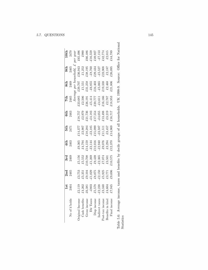
5.7. QUESTIONS 145
1st
2nd
3rd
4th
5th
6th
7th
8th
9th
10th
Noofh�holds
2464
2465
2469
2463
2471
2463
2465
2469
2465
2470
Averageperhousehold,£peryear
OriginalIncome
£2,119
£3,753
£5,156
£9,365
£14,377
£18,757
£23,685
£29,707
£36,943
£65,496
Cashbene�ts
£4,262
£5,351
£5,552
£4,794
£3,907
£2,979
£2,506
£1,551
£1,252
£990
Grossincome
£6,381
£9,104
£10,708
£14,159
£18,284
£21,736
£26,191
£31,258
£38,195
£66,486
DirTaxes
-£803
-£1,029
-£1,269
-£2,144
-£3,185
-£4,183
-£5,414
-£6,855
-£8,760
-£16,559
Dispincome
£5,578
£8,075
£9,439
£12,016
£15,099
£17,554
£20,777
£24,403
£29,434
£49,927
Indirecttaxes
-£2,238
-£2,150
-£2,365
-£2,940
-£3,587
-£4,055
-£4,611
-£5,065
-£5,527
-£7,153
Post-taxincome
£3,340
£5,925
£7,074
£9,076
£11,511
£13,498
£16,166
£19,338
£23,908
£42,774
Bene�tsinkind
£4,604
£3,771
£3,501
£3,294
£3,457
£3,219
£2,787
£2,468
£2,187
£2,015
Finalincome
£7,945
£9,696
£10,575
£12,370
£14,969
£16,717
£18,953
£21,806
£26,095
£44,789
Table5.6:Averageincome,taxesandbene�tsbydecilegroupsofallhouseholds.UK1998-9.Source:O¢ceforNational
Statistics
146 CHAPTER 5. FROM THEORY TO PRACTICE
(b) Repeat the exercise for the cases � = 0:5 and � = 2. Do you get thesame relationship between measured inequality and �?
(c) Repeat the exercise for the case where each family is weighted accord-ing to the number of individuals in it. Does the reweighting a¤ectthe results?[See the �le �Equivalence scales and weighting �on thewebsite for the answers. See also Coulter et al. (1992b) for furtherdiscussion.]
4. Suppose you have income data which has been grouped into three intervals:($0,$2000), ($2000,$4000), ($4000,$6000). There are 1000 individuals ineach interval and the mean of each interval is at the midpoint. Draw thelower-bound and upper-bound Lorenz curves as described on page 120.
5. Compute the mean and variance for a split histogram distribution over aninterval [a; b]: i.e. a distribution for which the density is a constant f1 fora � y < �y and f2 for �y � y < b. Given the US data in Table 5.1 (see �le�IRS Income Distribution�on the website) �nd the numbers f1 and f2 foreach interval.
6. Show that you can write the formula for Gini coe¢ cient on page 110 asG =
Pni=1 wiy(i) where the w1; w2; :::; wn are weights for each income from
the lowest (i = 1) to the highest (i = n).
� What is the formula for wi?� If there is a small income transfer of �y from person i to person jwhat is the impact on G according to this formula?
� Suppose a six-person economy has income distribution A given inTable 3.3 (page 63). Use your solution for �y to evaluate the e¤ecton Gini of switching to distribution B for the East, for the West andfor the economy as a whole.
� Suppose a six-person economy has income distribution A given inTable 3.4. Again use your solution for �y to evaluate the e¤ect onGini of switching to distribution B for the East, for the West and forthe economy as a whole. Why do you get a rather di¤erent answerfrom the previous case?
7. For the same data set as in question 5 verify the lower bound and theupper bound estimates of the Atkinson index A0:5 given in Table 5.2.
8. Apply a simple test to the data in Table 5.7 (also available in �le �Jiangsu�on the website) to establish whether or not the lognormal model is appro-priate in this case. What problems are raised by the �rst interval here?(Kmietowicz and Ding 1993).
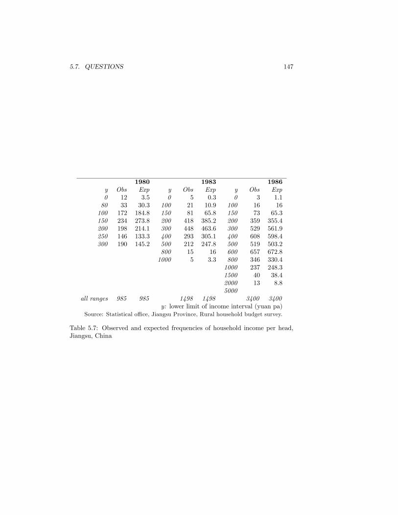
5.7. QUESTIONS 147
1980 1983 1986y Obs Exp y Obs Exp y Obs Exp0 12 3.5 0 5 0.3 0 3 1.180 33 30.3 100 21 10.9 100 16 16100 172 184.8 150 81 65.8 150 73 65.3150 234 273.8 200 418 385.2 200 359 355.4200 198 214.1 300 448 463.6 300 529 561.9250 146 133.3 400 293 305.1 400 608 598.4300 190 145.2 500 212 247.8 500 519 503.2
800 15 16 600 657 672.81000 5 3.3 800 346 330.4
1000 237 248.31500 40 38.42000 13 8.85000
all ranges 985 985 1498 1498 3400 3400y: lower limit of income interval (yuan pa)
Source: Statistical o¢ ce, Jiangsu Province, Rural household budget survey.
Table 5.7: Observed and expected frequencies of household income per head,Jiangsu, China

148 CHAPTER 5. FROM THEORY TO PRACTICE
Appendix A
Technical Appendix
A.1 Overview
This appendix assembles some of the background material for results in themain text and covers some important related points that are of a more technicalnature. The topics covered, section by section, are as follows:
� Standard properties of inequality measures both for general income dis-tributions (continuous and discrete) and for speci�c distributions.
� The properties of some important standard functional forms of distribu-tions, focusing mainly upon the lognormal and Pareto families.
� Interrelationships amongst important speci�c inequality measures
� Inequality decomposition by population subgroup.
� Inequality decomposition by income components.
� Negative incomes.
� Estimation problems for (ungrouped) microdata.
� Estimation problems for grouped data, where the problem of interpolationwithin groups is treated in depth.
� Using the website to work through practical examples.
A.2 Measures and their properties
This section reviews the main properties of standard inequality indices; it alsolists the conventions in terminology and notation used throughout this appen-dix. Although all the de�nitions could be expressed concisely in terms of the
149
150 APPENDIX A. TECHNICAL APPENDIX
distribution function F , for reasons of clarity I list �rst the terminology and de-�nitions suitable speci�cally for discrete distributions with a �nite population,and then present the corresponding concepts for continuous distributions.
Discrete Distributions
The basic notation required is as follows. The population size is n, and theincome of person i is yi, i = 1; :::; n. The arithmetic mean and the geometricmean are de�ned, respectively, as
�y =1
n
nXi=1
yi:
y� = exp
1
n
nXi=1
log yi
!= [y1y2y3:::yn]
1=n:
Using the arithmetic mean we may de�ne the share of person i in total incomeas si = yi= [n�y].Table A.1 lists the properties of many inequality measures mentioned in this
book, in the following format:
� A general de�nition of inequality measure given a discrete income distri-bution
� The maximum possible value of each measure on the assumption that allincomes are non-negative. Notice in particular that for " � 1 the maximumvalue of A" and D" is 1, but not otherwise. The minimum value of eachmeasure is zero with the exception of the Her�ndahl index for which theminimum is 1
n .
� The transfer e¤ect for each measure: the e¤ect of the transfer of an in�n-itesimal income transfer from person i to person j.
Continuous distributions
The basic notation required is as follows. If y is an individual�s income F (y)denotes the proportion of the population with income less than or equal to y.The operator
Rimplies that integration is performed over the entire support of
y; i.e. over [0;1) or, equivalently for F , over the interval [0; 1]. The arithmeticmean and the geometric mean are de�ned as
�y =
Zy dF;
y� = exp
�Zlog y dF
�:
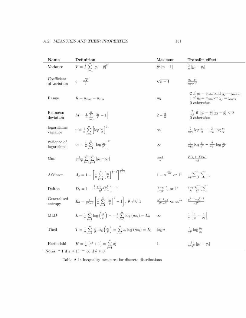
A.2. MEASURES AND THEIR PROPERTIES 151
Name De�nition Maximum Transfer e¤ect
Variance V = 1n
nPi=1
[yi � �y]2 �y2 [n� 1] 2n [yj � yi]
Coe¢ cientof variation
c =pV�y
pn� 1 yj�yi
n�ypV
Range R = ymax � ymin n�y2 if yi = ymin and yj = ymax,1 if yi = ymin or yj = ymax,0 otherwise
Rel.meandeviation
M = 1n
nPi=1
���yi�y � 1��� 2� 2n
2n�y if [yi � �y] [yj � �y] < 00 otherwise
logarithmicvariance
v = 1n
nPi=1
hlog yi�y
i21 2
nyjlog
yj�y �
2nyi
log yi�y
variance oflogarithms
v1 =1n
nPi=1
hlog yi
y�
i21 2
nyjlog
yjy� �
2nyi
log yiy�
Gini 12n2�y
nPi=1
nPj=1
jyi � yj j n�1n
F (yj)�F (yi)n�y
Atkinson A" = 1��1n
nPi=1
hyi�y
i1�"� 11�"
1� n�"1�" or 1�
y�"i �y�"j
n�y1�"[1�A"]�"
Dalton D" = 1�1n
Pni=1 y
1�"i � 1
�y1�" � 11�n�"1��y"�1 or 1
� 1�"n
y�"i �y�"j
�y1�"�1
Generalisedentropy
E� =1
�2��
�1n
nPi=1
hyi�y
i�� 1�; � 6= 0; 1 n��1�1
�2�� or 1�� y��1i �y��1j
n�y�
MLD L = 1n
nPi=1
log��yyi
�= � 1
n
nPi=1
log (nsi) = E0 1 1n
h1yi� 1
yj
iTheil T = 1
n
nPi=1
yi�y log
�yi�y
�=
nPi=1
si log (nsi) = E1 log n 1n�y log
yjyi
Her�ndahl H = 1n
�c2 + 1
�=
nPi=1
s2i 1 2n2�y2 [yj � yi]
Notes: � 1 if " � 1; �� 1 if � � 0.
Table A.1: Inequality measures for discrete distributions
152 APPENDIX A. TECHNICAL APPENDIX
If the density function f (�) is everywhere well-de�ned then these de�nitions canbe written equivalently as
�y =Ryf (y) dy;
y� = exp
�Zlog y f (y) dy
�:
From the above we may de�ne the proportion of total income received by personswho have an income less than or equal to y as
�(y) =1
�y
Z y
0
zdF (z):
The Lorenz curve is the graph of (F;�).Table A.2 performs the rôle of Table A.1 for the case of continuous distribu-
tions as well as other information: to save space not all the inequality measureshave been listed in both tables. The maximum value for the inequality measuresin this case can be found by allowing n!1 in column 3 of Table A.1. In orderto interpret Table A.2 you also need the standard normal distribution function
N(x) =1p2�
Z x
�1e�
12u
2
du;
provided in most spreadsheet software and tabulated in Lindley and Miller(1966) and elsewhere; N�1(�) denotes the inverse function corresponding toN(�). In summary Table A.2 gives:
� A de�nition of inequality measures for continuous distributions.
� The formula for the measure given that the underlying distribution islognormal.
� The formula given that the underlying distribution is Pareto (type I).
A.3 Functional forms of distribution
We begin this section with a simple listing of the principal properties of thelognormal and Pareto distributions in mathematical form. This is deliberatelybrief since a full verbal description is given in Chapter 4, and the formulas ofinequality measures for these distributions are in Table A.2.
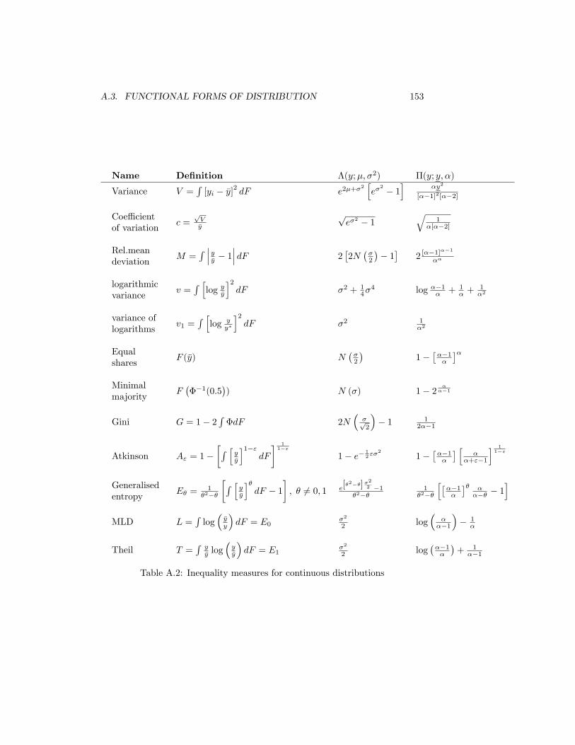
A.3. FUNCTIONAL FORMS OF DISTRIBUTION 153
Name De�nition �(y;�; �2) �(y; y; �)
Variance V =R[yi � �y]2 dF e2�+�
2he�
2 � 1i
�y2
[��1]2[��2]
Coe¢ cientof variation
c =pV�y
pe�2 � 1
q1
�[��2]
Rel.meandeviation
M =R ���y�y � 1��� dF 2
�2N��2
�� 1�
2 [��1]��1
��
logarithmicvariance
v =R hlog y�y
i2dF �2 + 1
4�4 log ��1� + 1
� +1�2
variance oflogarithms
v1 =R hlog y
y�
i2dF �2 1
�2
Equalshares
F (�y) N��2
�1�
���1�
��Minimalmajority
F���1(0:5
�) N (�) 1� 2 �
��1
Gini G = 1� 2R�dF 2N
��p2
�� 1 1
2��1
Atkinson A" = 1��R h
y�y
i1�"dF
� 11�"
1� e� 12 "�
2
1����1�
� h�
�+"�1
i 11�"
Generalisedentropy
E� =1
�2��
�R hy�y
i�dF � 1
�; � 6= 0; 1 e[�
2��]�2
2 �1�2��
1�2��
h���1�
�� ���� � 1
iMLD L =
Rlog��yy
�dF = E0
�2
2 log�
���1
�� 1
�
Theil T =Ry�y log
�y�y
�dF = E1
�2
2 log���1�
�+ 1
��1
Table A.2: Inequality measures for continuous distributions
154 APPENDIX A. TECHNICAL APPENDIX
The lognormal distribution
The basic speci�cation is:
F (y) = ��y; �; �2
�=
Z y
0
1p2� �x
exp
�� 1
2�2[log x� �]2
�dx;
�(y) = ��y; �+ �2; �2
�;
�y = e�+12�
2
;
y� = e�:
where � and � are parameters; and the Lorenz curve is given by:
� = N�N�1 (F )� �
�The Pareto distribution (type I)
The basic speci�cation is:
F (y) = �(y; y; �) = 1��y=y��;
�(y) = �(y; y; �� 1);
�y =�
�� 1y;
y� = e1=�y:
where � and y are parameters. Clearly the density function is
f(y) =�y�
y�+1
and the Lorenz curve is given by:
� = 1� [1� F ]��1� :
The last equation may be used to give a straightforward method of interpola-tion between points on a Lorenz curve. Given two observed points (F0;�0),(F1;�1), then for an arbitrary intermediate value F (where F0 < F < F1), thecorresponding intermediate �-value is:
�(y) = exp
log 1�F (y)1�F0 log 1��11��0
log 1�F11��0
!
However, if this formula is used to interpolate between observed points whenthe underlying distribution is not Pareto type I then the following di¢ culty mayarise. Suppose the class intervals used in grouping the data fa1; a2; a3; :::; ak; ak+1g,the proportions of the population in each group ff1; f2; f3; :::; fkg, and the aver-age income of each group f�1; �2; �3; :::; �kg, are all known. Then, as describedon page 120, a �maximum inequality� Lorenz curve may be drawn through
A.3. FUNCTIONAL FORMS OF DISTRIBUTION 155
the observed points using this information. But the above Pareto interpolationformula does not use the information on the as, and the resulting interpolatedLorenz curve may cross the maximum inequality curve. Methods that use all theinformation about each interval are discussed below in the section �Estimationproblems�on page 172.
Van der Wijk�s law As mentioned in Chapter 4 the Pareto type I distribu-tion has an important connection with van der Wijk�s law. First we shall derivethe average income z(y) of everyone above an income level y. This is
z(y) =
R1yuf(u)duR1
yf(u)du
= �y1� �(y)1� F (y) :
From the above, for the Pareto distribution (Type I) we have
z(y) =�
�� 1y�y=y���1 �
y=y���
=�
�� 1y:
Hence the average income above the level y is proportional to y itself.Now let us establish that this result is true only for the Pareto (type I)
distribution within the class of continuous distributions. Suppose for some dis-tribution it is always true that z(y) = y where is a constant; then, onrearranging, we have Z 1
y
uf(u)du = y
Z 1
y
f(u)du;
where f(�) is unknown. Di¤erentiate this with respect to y:
�yf(y) = � yf(y) + [1� F (y)] :
De�ne � = =[ � 1]; then, rearranging this equation, we have
yf(y) + �F (y) = �:
Since f(y) = dF (y)=dy, this can be treated as a di¤erential equation in y.Solving for F , we have
y�F (y) = y� +B;
where B is a constant. Since F�y�= 0 when we have B = �y�. So
F (y) = 1��y=y��:
156 APPENDIX A. TECHNICAL APPENDIX
Other functional forms
As noted in Chapter 4 many functional forms have been used other than thelognormal and the Pareto. Since there is not the space to discuss these in thesame detail, the remainder of this section simply deals with the main types; indi-cating family relationships, and giving the moments about zero where possible.(If you have the rth moment about zero, then many other inequality measuresare easily calculated; for example,
A" = 1�[�0r]
1=r
�01;
where �0r is the rth moment about zero, r = 1� " and �01 = �y.)We deal �rst with family relations of the Pareto distribution. The distrib-
ution function of the general form, known as the type III Pareto distribution,may be written as
F (y) = 1� e��y
[ y + �]� ;
where � > 0; � � 0; > 0 and y + � � 0. By putting � = 0 and � = 1 inthe above equation we obtain the Pareto type II distribution (see below). Byputting � = � = 0 and = 1=y in the type III distribution we get the Paretotype I distribution, �(y; y; �). Rasche et al. (1980) suggested a functional formfor the Lorenz curve as follows:
� = [1� [1� F ]a]1b :
Clearly this expression also contains the Pareto type I distribution as a specialcase.The Rasche et al. (1980) form is somewhat intractable, and so in response
Gupta (1984) and Rao and Tam (1987) have suggested the following:
� = F abF�1; a � 1; b > 1:
(Gupta�s version has a � 1.) A comparative test of these and other forms isalso provided by Rao and Tam (1987).Singh and Maddala (1976) suggested as a useful functional form the follow-
ing:
F (y) = 1� 1
[1 + y� ]� ;
where �, �, are positive parameters. From this we can derive the followingspecial cases.
� If � = 1 we have the Pareto type II distribution.
� If = [1=�] k� and � ! 1 then the Weibull distribution is generated:F (y) = 1 � exp
��[ky]�
�. The rth moment about zero is given by �0r =
k�r�(1 + r=�), where �(�) is the Gamma function de�ned by �(x) =Ruxe�udu.
A.3. FUNCTIONAL FORMS OF DISTRIBUTION 157
� A special case of the Weibull may be found when � = 1, namely theexponential distribution F (y) = 1 � exp(�ky). Moments are given byk�r�(1 + r) which for integral values of r is simply k�rr!.
� If � = 1 and = y�� , then we �nd Fisk�s sech2-distribution:
F (y) = 1�"1 +
�y
y
��#�1;
with the rth moment about zero given by
�0r = ryr�
� sin�r��
� ; �� < r < �:
Furthermore the upper tail of the distribution is asymptotic to a con-ventional Pareto type-I distribution with parameters y and � (for lowvalues of y the distribution approximates to a reverse Pareto distribu-tion � see Fisk (1961), p.175. The distribution gets its name from the
transformation�y=y��= ex, whence the transformed density function is
f(x) = ex=[1 + ex]2, a special case of the logistic function.
The sech2-distribution can also be found as a special case of the Champer-nowne distribution:
F (y) = 1� 1�tan�1
sin �
cos � +�y=y��!
where � is a parameter lying between �� and � (see Champernowne 1953, Fisk1961). This likewise approximates the Pareto type I distribution in its uppertail and has the following moments about zero:
�0r = yr�
�
sin�r��
�sin�r��
� ; �� < r < �:
The required special case is found by letting � ! 0.The Yule distribution can be written either in general form with density
functionf(y) = AB�(y; �+ 1)
where B�(y; � + 1) is the incomplete Beta functionR �0uy�1[1 � u]�du, � > 0
and 0 < � � 1, or in its special form with � = 1, where the frequency is thenproportional to the complete Beta function B(y; �+ 1).1 Its moments are
�0r =nXi=1
�n!
�� n�n;r ; � > r
1The analytical properties of the Beta and Gamma functions are discussed in many textson statistics, for example Berry and Lindgren (1996), Freund (2003).
158 APPENDIX A. TECHNICAL APPENDIX
where
�n;r =
8>>>>><>>>>>:[�1]r�n
nXi=1
nXj=1
nXk=j
:::[ijk:::]| {z }r�n terms
if n < r
1 if n = r
The Yule distribution in its special form approximates the distribution�(y; �(�)1=�; �)in its upper tail. A further interesting property of this special form is that fora discrete variable it satis�es van der Wijk�s law.We now turn to a rich family of distributions of which two members have
been used to some extent in the study of income distribution � the Pearsoncurves. The Pearson type I is the Beta distribution with density function:
f(y) =y� [1� y]�
B(�; �)
where 0 < y < 1,2 and �; � > 0. The rth moment about zero can be writtenB(� + r; �)=B(�; �) or as �(� + r)�(� + �)=[�(�)�(� + � + r)]. The Gammadistribution is of the type III of the Pearson family:
f(y) =��
�(�)y��1e��y;
where �; � > 0. The moments are given by
�0r = ��r�(�+ r)
�(�):
Three interesting properties of the Gamma function are as follows. Firstly, byputting � = 1, we �nd that it has the exponential distribution as a special case.Secondly, suppose that � = 1, and that y has the Gamma distribution with� = �1 while w has the Gamma distribution with � = �2. Then the sum w+ yalso has the Gamma distribution with � = �1+�2: a property that is obviouslyuseful if one is considering, say, the decomposition of income into constituentparts such as earned and unearned income. Thirdly, a Beta distribution with ahigh parameter � looks very similar to a Gamma distribution with high valuesof parameters �, �. This can be seen from the formula for the moments. Forhigh values of x and any constant k it is the case that �(x)=�(x + k) ' x�k.Hence the moments of the B-distribution approximate to [�+�]�r�(�+r)=�(�).The two-parameter Gamma distribution and the three-parameter Singh-
Maddala distribution can each be shown to be a particular case of the four-parameter Generalised Beta Distribution of the second kind for which the den-sity is:
f (y) =� �y���1
B (�; �+ 1) [1 + y� ]�+�+1
2This restriction means that y must be normalised by dividing it by its assumed maximumvalue.
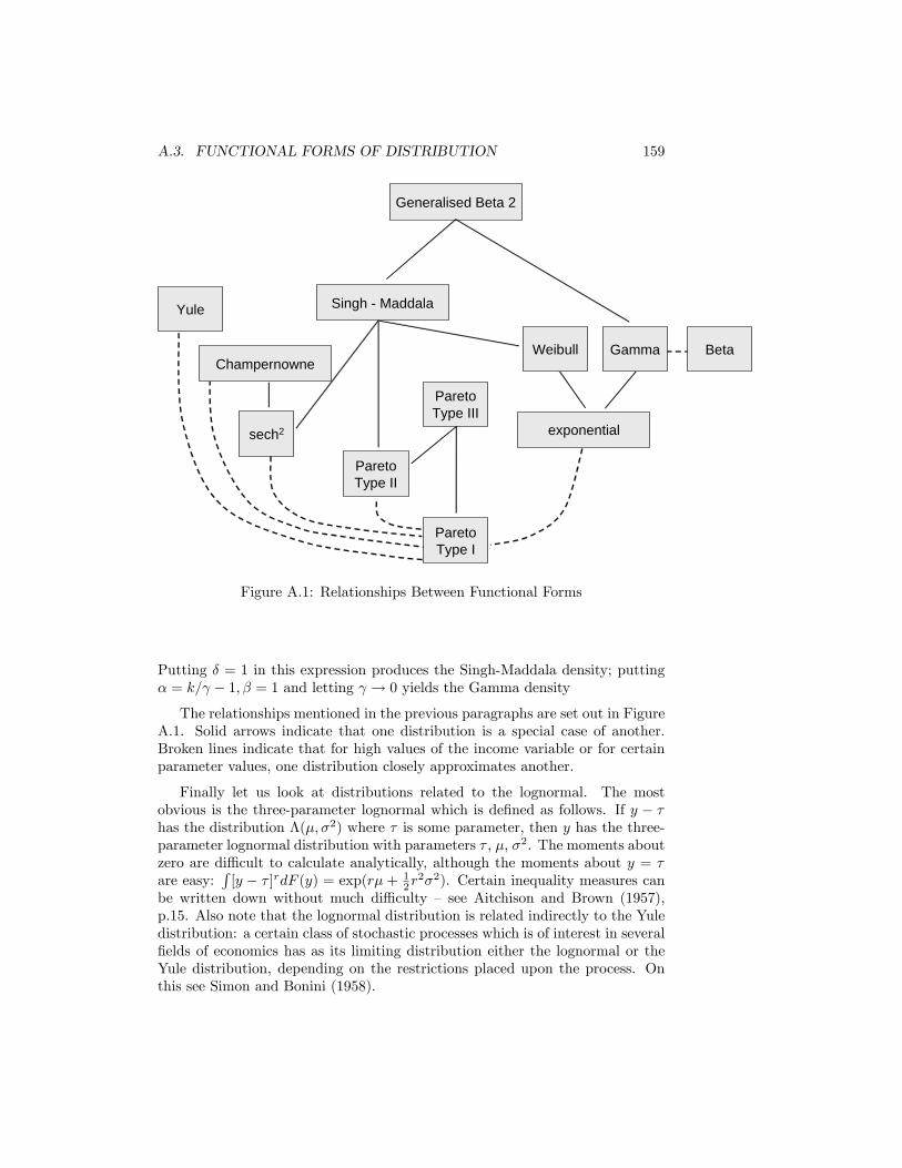
A.3. FUNCTIONAL FORMS OF DISTRIBUTION 159
ParetoType II
ParetoType III
Champernowne
Singh Maddala
exponential
Weibull
Yule
Gamma Beta
Generalised Beta 2
sech2
ParetoType I
Figure A.1: Relationships Between Functional Forms
Putting � = 1 in this expression produces the Singh-Maddala density; putting� = k= � 1; � = 1 and letting ! 0 yields the Gamma density
The relationships mentioned in the previous paragraphs are set out in FigureA.1. Solid arrows indicate that one distribution is a special case of another.Broken lines indicate that for high values of the income variable or for certainparameter values, one distribution closely approximates another.
Finally let us look at distributions related to the lognormal. The mostobvious is the three-parameter lognormal which is de�ned as follows. If y � �has the distribution �(�; �2) where � is some parameter, then y has the three-parameter lognormal distribution with parameters � , �, �2. The moments aboutzero are di¢ cult to calculate analytically, although the moments about y = �are easy:
R[y � � ]rdF (y) = exp(r� + 1
2r2�2). Certain inequality measures can
be written down without much di¢ culty � see Aitchison and Brown (1957),p.15. Also note that the lognormal distribution is related indirectly to the Yuledistribution: a certain class of stochastic processes which is of interest in several�elds of economics has as its limiting distribution either the lognormal or theYule distribution, depending on the restrictions placed upon the process. Onthis see Simon and Bonini (1958).
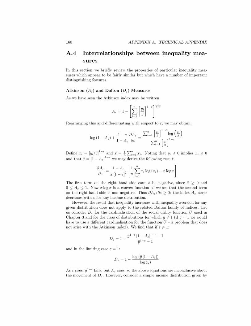
160 APPENDIX A. TECHNICAL APPENDIX
A.4 Interrelationships between inequality mea-sures
In this section we brie�y review the properties of particular inequality mea-sures which appear to be fairly similar but which have a number of importantdistinguishing features.
Atkinson (A") and Dalton (D") Measures
As we have seen the Atkinson index may be written
A" = 1�"
nXi=1
�yi�y
�1�"# 11�"
Rearranging this and di¤erentiating with respect to ", we may obtain:
log (1�A") +1� "1�A"
@A"@"
=
Pni=1
hyi�y
i1�"log�yi�y
�Pn
i=1
hyi�y
i1�"De�ne xi = [yi=�y]
1�" and �x = 1n
Pni=1 xi. Noting that yi � 0 implies xi � 0
and that �x = [1�A"]1�" we may derive the following result:
@A"@"
=1�A"�x [1� "]2
"1
n
nXi=1
xi log (xi)� �x log �x#
The �rst term on the right hand side cannot be negative, since �x � 0 and0 � A" � 1. Now x log x is a convex function so we see that the second termon the right hand side is non-negative. Thus @A"=@" � 0: the index A" neverdecreases with " for any income distribution.However, the result that inequality increases with inequality aversion for any
given distribution does not apply to the related Dalton family of indices. Letus consider D" for the cardinalisation of the social utility function U used inChapter 3 and for the class of distributions for which �y 6= 1 (if �y = 1 we wouldhave to use a di¤erent cardinalisation for the function U �a problem that doesnot arise with the Atkinson index). We �nd that if " 6= 1:
D" = 1��y1�" [1�A"]1�" � 1
�y1�" � 1
and in the limiting case " = 1:
D" = 1�log (�y [1�A1])
log (�y)
As " rises, �y1�" falls, but A" rises, so the above equations are inconclusive aboutthe movement of D". However, consider a simple income distribution given by
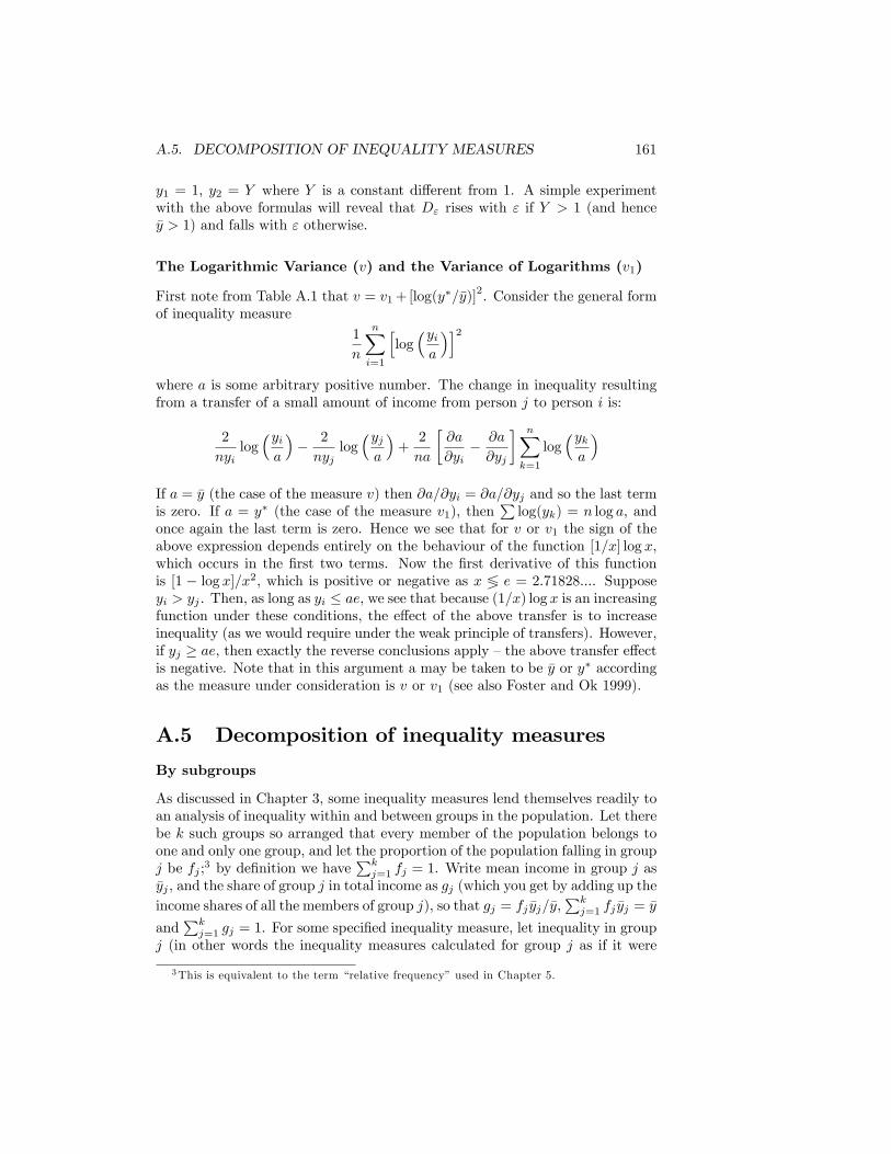
A.5. DECOMPOSITION OF INEQUALITY MEASURES 161
y1 = 1, y2 = Y where Y is a constant di¤erent from 1. A simple experimentwith the above formulas will reveal that D" rises with " if Y > 1 (and hence�y > 1) and falls with " otherwise.
The Logarithmic Variance (v) and the Variance of Logarithms (v1)
First note from Table A.1 that v = v1+[log(y�=�y)]
2. Consider the general formof inequality measure
1
n
nXi=1
hlog�yia
�i2where a is some arbitrary positive number. The change in inequality resultingfrom a transfer of a small amount of income from person j to person i is:
2
nyilog�yia
�� 2
nyjlog�yja
�+2
na
�@a
@yi� @a
@yj
� nXk=1
log�yka
�If a = �y (the case of the measure v) then @a=@yi = @a=@yj and so the last termis zero. If a = y� (the case of the measure v1), then
Plog(yk) = n log a, and
once again the last term is zero. Hence we see that for v or v1 the sign of theabove expression depends entirely on the behaviour of the function [1=x] log x,which occurs in the �rst two terms. Now the �rst derivative of this functionis [1 � log x]=x2, which is positive or negative as x 7 e = 2:71828:::. Supposeyi > yj . Then, as long as yi � ae, we see that because (1=x) log x is an increasingfunction under these conditions, the e¤ect of the above transfer is to increaseinequality (as we would require under the weak principle of transfers). However,if yj � ae, then exactly the reverse conclusions apply �the above transfer e¤ectis negative. Note that in this argument a may be taken to be �y or y� accordingas the measure under consideration is v or v1 (see also Foster and Ok 1999).
A.5 Decomposition of inequality measures
By subgroups
As discussed in Chapter 3, some inequality measures lend themselves readily toan analysis of inequality within and between groups in the population. Let therebe k such groups so arranged that every member of the population belongs toone and only one group, and let the proportion of the population falling in groupj be fj ;3 by de�nition we have
Pkj=1 fj = 1. Write mean income in group j as
�yj , and the share of group j in total income as gj (which you get by adding up theincome shares of all the members of group j), so that gj = fj �yj=�y,
Pkj=1 fj �yj = �y
andPk
j=1 gj = 1. For some speci�ed inequality measure, let inequality in groupj (in other words the inequality measures calculated for group j as if it were
3This is equivalent to the term �relative frequency�used in Chapter 5.
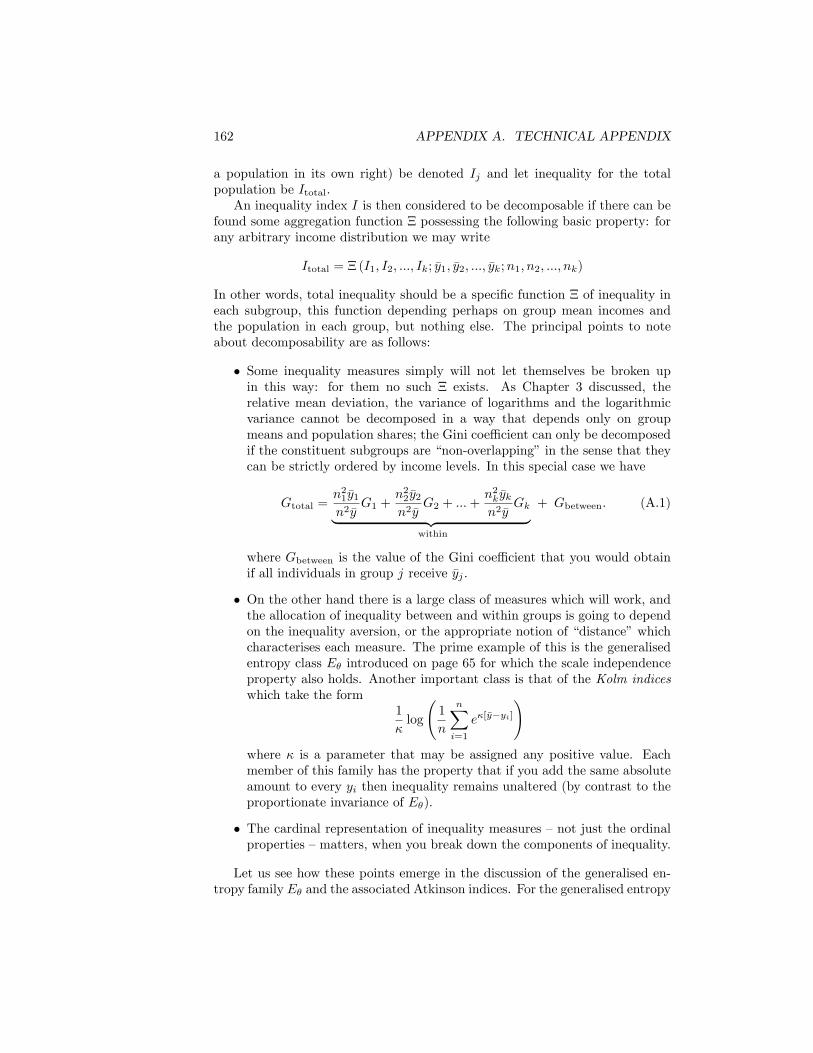
162 APPENDIX A. TECHNICAL APPENDIX
a population in its own right) be denoted Ij and let inequality for the totalpopulation be Itotal.An inequality index I is then considered to be decomposable if there can be
found some aggregation function � possessing the following basic property: forany arbitrary income distribution we may write
Itotal = �(I1; I2; :::; Ik; �y1; �y2; :::; �yk;n1; n2; :::; nk)
In other words, total inequality should be a speci�c function � of inequality ineach subgroup, this function depending perhaps on group mean incomes andthe population in each group, but nothing else. The principal points to noteabout decomposability are as follows:
� Some inequality measures simply will not let themselves be broken upin this way: for them no such � exists. As Chapter 3 discussed, therelative mean deviation, the variance of logarithms and the logarithmicvariance cannot be decomposed in a way that depends only on groupmeans and population shares; the Gini coe¢ cient can only be decomposedif the constituent subgroups are �non-overlapping�in the sense that theycan be strictly ordered by income levels. In this special case we have
Gtotal =n21�y1n2�y
G1 +n22�y2n2�y
G2 + :::+n2k�ykn2�y
Gk| {z }within
+ Gbetween: (A.1)
where Gbetween is the value of the Gini coe¢ cient that you would obtainif all individuals in group j receive �yj .
� On the other hand there is a large class of measures which will work, andthe allocation of inequality between and within groups is going to dependon the inequality aversion, or the appropriate notion of �distance�whichcharacterises each measure. The prime example of this is the generalisedentropy class E� introduced on page 65 for which the scale independenceproperty also holds. Another important class is that of the Kolm indiceswhich take the form
1
�log
1
n
nXi=1
e�[�y�yi]
!where � is a parameter that may be assigned any positive value. Eachmember of this family has the property that if you add the same absoluteamount to every yi then inequality remains unaltered (by contrast to theproportionate invariance of E�).
� The cardinal representation of inequality measures �not just the ordinalproperties �matters, when you break down the components of inequality.
Let us see how these points emerge in the discussion of the generalised en-tropy family E� and the associated Atkinson indices. For the generalised entropy
A.5. DECOMPOSITION OF INEQUALITY MEASURES 163
class E� the inequality aggregation result can be expressed in particularly simpleterms. If we de�ne4
Ibetween =1
�2 � �
24 kXj=1
fj
��yj�y
��� 1
35and
Iwithin =kXj=1
wjIj , where wj = g�j f1��j
then for any generalised entropy measure we have:
Itotal = Ibetween + Iwithin
From these three equations we may note that in the case of the generalisedentropy class
� total inequality is a simple additive function of between-group and within-group inequality,
� the between-group component of inequality is found simply by assumingthat everyone within a group receives that group�s mean income: it isindependent of redistribution within any of the j groups.
� within-group inequality is a weighted average of inequality in each sub-group, although the weights wj do not necessarily sum to one.
� the within-group component weights will only sum to one if � = 0 (thecase of the Mean Logarithmic Deviation L) or if � = 1 (the case of Theil�sindex T )..
The Atkinson index A" is ordinally equivalent to E� for " = 1� � > 0 (theywill always rank any set of Lorenz curves in the same order, as we noted inChapter 3); in fact we have
A" =
8<: 1����2 � �
�E� + 1
�1=�for � 6= 0
A1 = 1� e�E0 for � = 0:
However, because this relationship is nonlinear, we do not have cardinal equiv-alence between the two indices; as a result we will get a di¤erent relationshipbetween total inequality and its components. We can �nd this relationship bysubstituting the last formula into the decomposition formula for the generalised
4Notice that this is the same as the expression given for the generalised entropy measure inTable A.1 for the case where fi = 1=n: in other words you can imagine the whole populationof size n as being composed of n groups each of size 1.
164 APPENDIX A. TECHNICAL APPENDIX
entropy measure above. If we do this then �for the case where I is the Atkinsonindex with parameter " �we get the following:
Ibetween = 1�
24 kXj=1
fj
��yj�y
�1�"35 11�"
Itotal = 1�"
nXi=1
1
n
�yi�y
�1�"# 11�"
[1� Itotal]1�" =h[1� Ibetween]1�" + [1� Iwithin]1�" � 1
iand from these we can deduce
Iwithin = 1�
241� kXj=1
f"j g1�"j
h[1� Ij ]1�" � 1
i35 11�"
To restate the point: the decomposition formula given here for the Atkinsonindex is di¤erent from that given on page 163 for the generalised entropy indexbecause one index is a nonlinear transformation of the other. Let us illustratethis further by taking a speci�c example using the two inequality measures,A2 and E�1, which are ordinally but not cardinally equivalent. We have thefollowing relationship:
A2 = 1�1
2E�1 + 1:
Applying this formula and using a self-explanatory adaptation of our earliernotation the allocation of the components of inequality is as follows:
E�1[within] =kXj=1
f2jgjE�1[j]
E�1[between] =1
2
24 kXj=1
f2jgj� 1
35E�1[total] = E�1[between] + E�1[within]
whereas
A2[total] =A2[between] +A2[within] �A2[between]A2[within]
1�A2[between]A2[within]
Now let us consider the situation in China represented in Table A.3. The toppart gives the mean income, population and inequality for each of the ten re-gions, and for urban and rural groups within each region. The bottom partof the table gives the corresponding values for A2 and E�1 broken down intowithin- and between-group components (by region) for urban and regional in-comes. Notice that
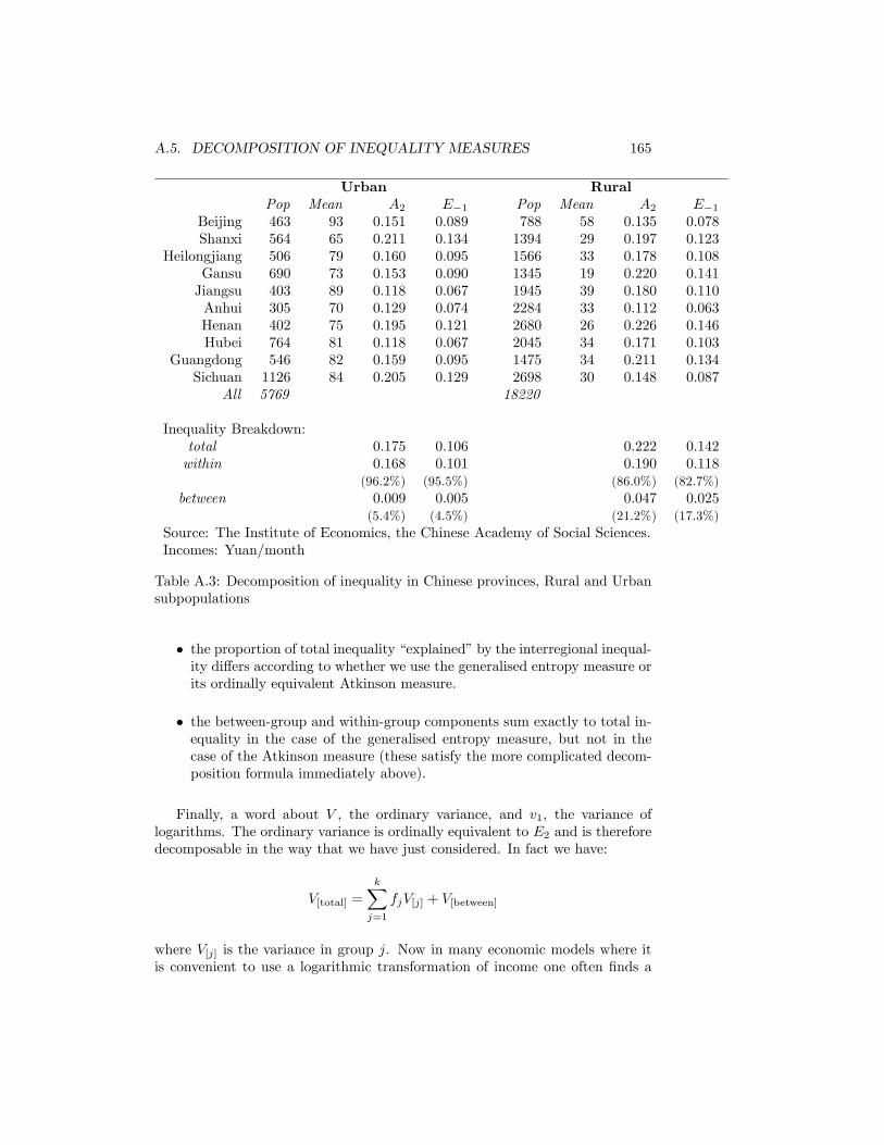
A.5. DECOMPOSITION OF INEQUALITY MEASURES 165
Urban RuralPop Mean A2 E�1 Pop Mean A2 E�1
Beijing 463 93 0.151 0.089 788 58 0.135 0.078Shanxi 564 65 0.211 0.134 1394 29 0.197 0.123
Heilongjiang 506 79 0.160 0.095 1566 33 0.178 0.108Gansu 690 73 0.153 0.090 1345 19 0.220 0.141Jiangsu 403 89 0.118 0.067 1945 39 0.180 0.110Anhui 305 70 0.129 0.074 2284 33 0.112 0.063Henan 402 75 0.195 0.121 2680 26 0.226 0.146Hubei 764 81 0.118 0.067 2045 34 0.171 0.103
Guangdong 546 82 0.159 0.095 1475 34 0.211 0.134Sichuan 1126 84 0.205 0.129 2698 30 0.148 0.087
All 5769 18220
Inequality Breakdown:total 0.175 0.106 0.222 0.142within 0.168 0.101 0.190 0.118
(96.2%) (95.5%) (86.0%) (82.7%)between 0.009 0.005 0.047 0.025
(5.4%) (4.5%) (21.2%) (17.3%)Source: The Institute of Economics, the Chinese Academy of Social Sciences.Incomes: Yuan/month
Table A.3: Decomposition of inequality in Chinese provinces, Rural and Urbansubpopulations
� the proportion of total inequality �explained�by the interregional inequal-ity di¤ers according to whether we use the generalised entropy measure orits ordinally equivalent Atkinson measure.
� the between-group and within-group components sum exactly to total in-equality in the case of the generalised entropy measure, but not in thecase of the Atkinson measure (these satisfy the more complicated decom-position formula immediately above).
Finally, a word about V , the ordinary variance, and v1, the variance oflogarithms. The ordinary variance is ordinally equivalent to E2 and is thereforedecomposable in the way that we have just considered. In fact we have:
V[total] =kXj=1
fjV[j] + V[between]
where V[j] is the variance in group j. Now in many economic models where itis convenient to use a logarithmic transformation of income one often �nds a
166 APPENDIX A. TECHNICAL APPENDIX
�decomposition�that looks something like this:
v1[total] =kXj=1
fjv1[j] + v1[between]
However, this is not a true inequality decomposition. To see why, consider themeaning of the between-group component in this case. We have
v1[between] =kXj=1
fj�log y�j � log y�
�2But, unlike the between-group component of the decomposition procedure weoutlined earlier, this expression is not independent of the distribution withineach group: for example if there were to be a mean-preserving income equal-isation in group j both the within-group geometric mean (y�j ) and the overallgeometric mean (y�) will be a¤ected. As mentioned above, you cannot properlydisentangle the within-group and between-group inequality components for thevariance of logarithms.
By income components
By contrast to the problem of decomposition by population subgroups there arerelatively few inequality measures that will allow a convenient breakdown bycomponent of income. However, the coe¢ cient of variation c and measures thatare ordinally equivalent to it (such as V and H) can be handled relatively easily.Nothing is lost by simplifying to a pairwise decomposition: let income be madeup of two components, A and B so that for any person: yi = yiA+yiB. Further,let c, cA, cB be, respectively, the value of the coe¢ cient of variation for totalincome, component A income and component B, let � be the overall amountof component A as a proportion of total income, and let � be the correlationcoe¢ cient between component A and component B of income. Then:
c2 = �2c2A + [1� �]2c2B + 2� [1� �] cAcB�
Note that this is well-de�ned even in the presence of negative income compo-nents.
A.6 Negative incomes
For a great many applications in economics it is convenient and reasonable toassume that incomes are non-negative. In fact most of the material in this bookhas proceeded on this basis. However, there are some important exceptions tothis: for example personal wealth (net worth) may be negative at various pointsof the lifecycle, individuals� incomes may contain substantial losses from selfemployed or unincorporated business activity.
A.6. NEGATIVE INCOMES 167
The possibility that even a few observations may be negative raises someissues of principle for inequality measurement. Many of the standard inequalitymeasures are simply unde�ned for negative incomes; furthermore there is asubstantial class of these measures that will not work even for zero incomes.However, the standard �ranking�tools such as quantiles and shares are well
de�ned for all incomes �positive, zero or negative �although they may need tobe interpreted with some care. For example the Parade diagram probably lookmuch the same as that depicted in �gure 1 of Chapter 2, but the axes will havebeen shifted vertically.To see how the shape of the Lorenz curve and the generalised Lorenz curve is
a¤ected by the presence of negative incomes recall that the slope of the Lorenzcurve is given by y=�y, and the slope of the generalised Lorenz curve by y. So,if there are some negative incomes, but the mean is still strictly positive, thenboth curves will initially pass below the horizontal axis (they will be downward-sloping for as long as incomes are negative), will be horizontal at the point wherezero income is encountered, and then will adopt a fairly conventional shape overthe rest of the diagram. If mean income is actually negative, then the Lorenzcurve will appear to be ��ipped vertically�(the generalised Lorenz curve is nota¤ected in this way).In fact the use of the conventional Lorenz curve is somewhat problematic in
the presence of negative incomes. For this reason it is sometimes to convenient touse the absolute Lorenz curve (Moyes 1987), which may be described as follows.The ordinary (or relative) Lorenz curve can be thought of as the generalised
Lorenz curve of the distribution�y1�y ;
y2�y ; :::;
yn�y
�and the absolute Lorenz curve
is the generalised Lorenz curve of the distribution (y1 � �y; y2 � �y; :::; yn � �y)The reason that many conventional inequality tools will not work in the pres-
ence of negative incomes can be seen from �evaluation function�h(�) introducedon page 108. Recall that many inequality measures can be de�ned in terms ofthe evaluation function. Consider for example the generalised entropy familywhich will have an evaluation function of the form
h(y) = Ay�:
This function � and hence the associated inequality measures � will be wellde�ned for all negative incomes for the special case where � is a positive integergreater than 1. However, this severely restricts the choice of �, because measureswith even moderately large values of � prove to be extraordinarily sensitive toincomes in the upper tail. This means, for example, that in estimating inequalityfrom a sample of microdata, one or two large incomes will drive the estimatesof inequality by themselves. The coe¢ cient of variation (� = 2) is the onlymember of the generalised entropy class that is likely to be of practical use.By contrast all the Kolm indices work with negative incomes; the h function
here ish(y) = Ae��y
(� > 0) which is well-de�ned for all values of y. Finally measures that are based
168 APPENDIX A. TECHNICAL APPENDIX
on absolute di¤erences �such as the Gini coe¢ cient and relative mean deviation�will also be able to cope with negative incomes.
A.7 Estimation problems
Micro Data
As noted in Chapter 5, point estimates of inequality measures from a samplecan be obtained just by plugging in the observations to the basic formulas givenin Chapters 3 and 4. For computation of point estimates of inequality usingunweighted micro-data there are very few operations involved:
� Transformation of the income variable h(yi) �the calculation of each termin the formula for J on page 109; the function h(�) typically involves takinglogs or raising to a power and so the calculation can usually be performedby standard built-in functions in spreadsheet software.
� Calculating mean income and the mean of the transformed variables (as inthe formula for J on page 109) �another standard spreadsheet operation.
� Sorting the data if you want to compute the Gini coe¢ cient (page 110) orplot Lorenz curves �again this is standard for spreadsheets.
The only further quali�cation that ought to be made is that in practice oneoften has to work with weighted data (the weights could be sampling weightsfor example). In this case associated with each observed income yi there is anon-negative weight wi; let us suppose the weights have been normalised so thatthey sum to 1. Then, instead of the J-formula on page 109, one computes
J =
nXi=1
wih(yi)
and instead of the formula for G on page 110 one computes5
G =1
�y
nXi=1
�iw(i)y(i)
where
�i = 2iX
j=1
w(j) � w(i) � 1:
This requires a little more care, of course, but is still within the capability ofstandard spreadsheets.
5 In line with our previous usage w(i) and y(i) denote the weight and income for observationi after the observations have been sorted in ascending order of incomes. Note that in eachcase you can recover the original formulas for J and G for the unweighted case by settingwi = 1=n everywhere.
A.7. ESTIMATION PROBLEMS 169
Now consider the standard errors of inequality estimates in the case of un-weighted data. As we noted on page 156 inequality measures can be expressedin terms of standard statistical moments. Correspondingly in situations wherewe are working with a sample fy1; y2; :::yng of n observations from a targetpopulation we will be interested in the sample moment about zero:
m0r =
1
n
nXi=1
yri :
Standard results give the expected value (mean) and variance of the samplestatistic m0
r:E (m0
r) = �0r
var (m0r) =
1
n
h�02r � [�0r]
2i
and an unbiased estimate of the sample variance of m is
cvar (m0r) =
1
n� 1
hm02r � [m0
r]2i
If the mean of the distribution is known and you have unweighted data, thenthis last formula gives you all you need to set up a con�dence interval for thegeneralised entropy measure E�. Writing r = � and substituting we get (in thisspecial case):
E� =1
�2 � �
�m0�
�y�� 1�
where �y is the known mean (�01).However, if the mean also has to be estimated from the sample (as m0
1), or ifwe wish to use a nonlinear transformation of m0
�, then the derivation of a con�-dence interval for the inequality estimate is a bit more complicated. Applying astandard result (Rao 1973) we may state that if is a di¤erentiable function ofm0r and m
01, then the expression
pn [ (m0
r;m01)� (�0r; �01)] is asymptotically
normally distributed thus:
N
0;
�@
@m0r
�2var (m0
r) + 2@
@m0r
@
@m01r
cov (m0r;m
01) +
�@
@m01
�2var (m0
1)
!:
Again, if one has to work with weighted data the formulas for the standarderrors will need to be modi�ed to take into account the weighting. A crucialpoint here is whether the weights themselves also should be treated as randomvariables �see the notes (page 193) for further discussion of this point.Finally let us consider the problem of estimating the density function from
a set of n sample observations. As explained on page 110 in Chapter 5, a simplefrequency count is unlikely to be useful. An alternative approach is to assumethat each sample observation gives some evidence of the underlying densitywithin a �window�around the observation. Then you can estimate F (y), the

170 APPENDIX A. TECHNICAL APPENDIX
density at some income value y, by specifying an appropriate Kernel functionK (which itself has the properties of a density function) and a window width(or �bandwidth�) w and computing the function
f̂(y) =1
w
nXi=1
K
�y � yiw
��the individual terms in the summation on the right-hand side can be seen ascontributions of the observations yi to the density estimate f̂(y). The simplehistogram is an example of this device � see for example Figure 5.5. All thesample observations that happen to lie on or above aj and below aj+1 contributeto the height of the horizontal line-segment in the interval (aj ; aj+1). In the casewhere all the intervals are of uniform width so that w = aj+1 � aj , we wouldhave
K
�y � yiw
�=
8<: 1 ifaj � y < aj+1 andaj � yi < aj+1
0 otherwise
However, this histogram rule is crude: each observation makes an �all or noth-ing� contribution to the density estimate. So it may be more useful to takea kernel function that is less drastic. For example K is often taken to be thenormal density so that
K
�y � yiw
�=
1p2�e�
12 [
y�yiw ]
2
The e¤ect of using the normal kernel is illustrated in Figure A.2 for the casewhere there are just four income observations. The upper part of Figure A.2illustrates the use of a fairly narrow bandwidth, and the lower part the case ofa fairly wide window: the kernel density for each of the observations y1:::y4 isillustrated by the lightly-drawn curves: the heavy curve depicts the resultantdensity estimate. There is a variety of methods for specifying the kernel functionK and for specifying the window width w (for example so as to make the widthof the window adjustable to the sparseness or otherwise of the data): these arediscussed in Silverman (1986) and Simono¤ (1996).Of course associated witheach kernel point estimate f̂(y) there will also be a sampling variance, but thattakes us beyond the scope of this book.
Grouped Data
Now let us suppose that you do not have micro-data to hand, but that it hasbeen presented in the form of income groups. There are three main issues to bediscussed.
� How much information do you have? Usually this turns on whether youhave three pieces of information about each interval (the interval bound-aries ai, ai+1, the relative frequency within the interval fi, and the inter-val mean �i) or two (the interval boundaries, and the frequency). We willbrie�y consider both situations.
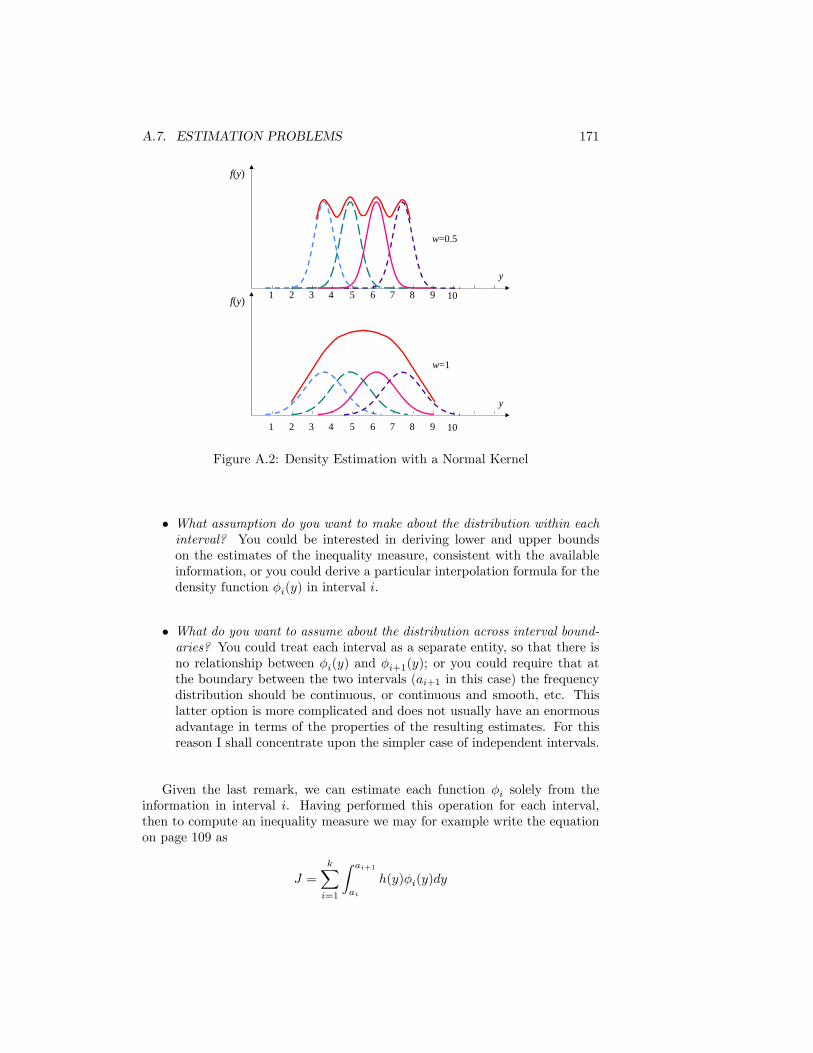
A.7. ESTIMATION PROBLEMS 171
y
f(y)
y
w=0.5
w=1
1 2 3 4 5 6 7 8 9 10
1 2 3 4 5 6 7 8 9 10
f(y)
Figure A.2: Density Estimation with a Normal Kernel
� What assumption do you want to make about the distribution within eachinterval? You could be interested in deriving lower and upper boundson the estimates of the inequality measure, consistent with the availableinformation, or you could derive a particular interpolation formula for thedensity function �i(y) in interval i.
� What do you want to assume about the distribution across interval bound-aries? You could treat each interval as a separate entity, so that there isno relationship between �i(y) and �i+1(y); or you could require that atthe boundary between the two intervals (ai+1 in this case) the frequencydistribution should be continuous, or continuous and smooth, etc. Thislatter option is more complicated and does not usually have an enormousadvantage in terms of the properties of the resulting estimates. For thisreason I shall concentrate upon the simpler case of independent intervals.
Given the last remark, we can estimate each function �i solely from theinformation in interval i. Having performed this operation for each interval,then to compute an inequality measure we may for example write the equationon page 109 as
J =
kXi=1
Z ai+1
ai
h(y)�i(y)dy
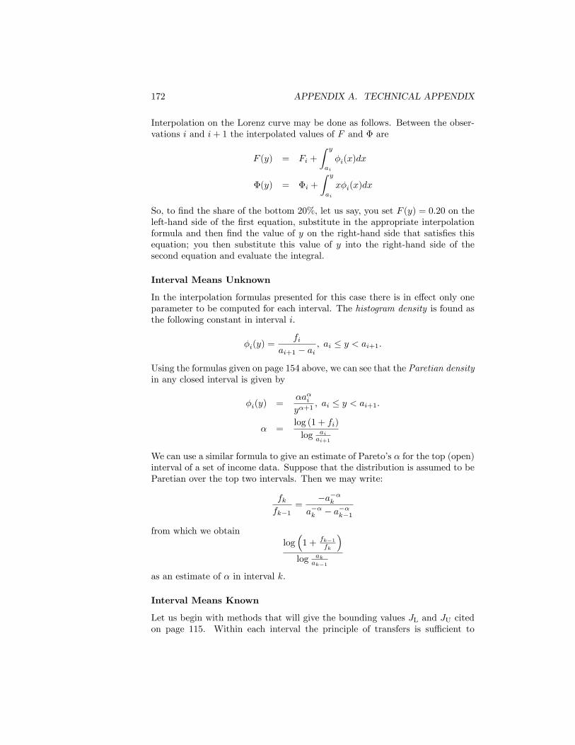
172 APPENDIX A. TECHNICAL APPENDIX
Interpolation on the Lorenz curve may be done as follows. Between the obser-vations i and i+ 1 the interpolated values of F and � are
F (y) = Fi +
Z y
ai
�i(x)dx
�(y) = �i +
Z y
ai
x�i(x)dx
So, to �nd the share of the bottom 20%, let us say, you set F (y) = 0:20 on theleft-hand side of the �rst equation, substitute in the appropriate interpolationformula and then �nd the value of y on the right-hand side that satis�es thisequation; you then substitute this value of y into the right-hand side of thesecond equation and evaluate the integral.
Interval Means Unknown
In the interpolation formulas presented for this case there is in e¤ect only oneparameter to be computed for each interval. The histogram density is found asthe following constant in interval i.
�i(y) =fi
ai+1 � ai; ai � y < ai+1:
Using the formulas given on page 154 above, we can see that the Paretian densityin any closed interval is given by
�i(y) =�a�iy�+1
; ai � y < ai+1:
� =log (1 + fi)
log aiai+1
We can use a similar formula to give an estimate of Pareto�s � for the top (open)interval of a set of income data. Suppose that the distribution is assumed to beParetian over the top two intervals. Then we may write:
fkfk�1
=�a��k
a��k � a��k�1
from which we obtainlog�1 + fk�1
fk
�log ak
ak�1
as an estimate of � in interval k.
Interval Means Known
Let us begin with methods that will give the bounding values JL and JU citedon page 115. Within each interval the principle of transfers is su¢ cient to
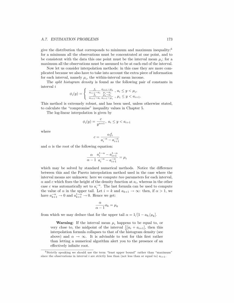
A.7. ESTIMATION PROBLEMS 173
give the distribution that corresponds to minimum and maximum inequality:6
for a minimum all the observations must be concentrated at one point, and tobe consistent with the data this one point must be the interval mean �i; for amaximum all the observations must be assumed to be at each end of the interval.Now let us consider interpolation methods: in this case they are more com-
plicated because we also have to take into account the extra piece of informationfor each interval, namely �i, the within-interval mean income.The split histogram density is found as the following pair of constants in
interval i
�i(y) =
(fi
ai+1�aiai+1��i�i�ai
, ai � y < �i,fi
ai+1�ai�i�aiai+1��i
, �i � y < ai+1.
This method is extremely robust, and has been used, unless otherwise stated,to calculate the �compromise�inequality values in Chapter 5.The log-linear interpolation is given by
�i(y) =c
y�+1; ai � y < ai+1
where
c =�fi
a��i � a��i+1and � is the root of the following equation:
�
�� 1a1��i � a1��i+1
a��i � a��i+1= �i
which may be solved by standard numerical methods. Notice the di¤erencebetween this and the Pareto interpolation method used in the case where theinterval means are unknown: here we compute two parameters for each interval,� and c which �xes the height of the density function at ai, whereas in the othercase c was automatically set to a��i . The last formula can be used to computethe value of � in the upper tail. Let i = k and ak+1 ! 1: then, if � > 1, wehave a��k+1 ! 0 and a1��k+1 ! 0. Hence we get:
�
�� 1ak = �k
from which we may deduce that for the upper tail � = 1=[1� ak=�k].
Warning: If the interval mean �i happens to be equal to, orvery close to, the midpoint of the interval 12 [ai + ai+1], then thisinterpolation formula collapses to that of the histogram density (seeabove) and � ! 1. It is advisable to test for this �rst ratherthan letting a numerical algorithm alert you to the presence of ane¤ectively in�nite root.
6Strictly speaking we should use the term �least upper bound� rather than �maximum�since the observations in interval i are strictly less than (not less than or equal to) ai+1.
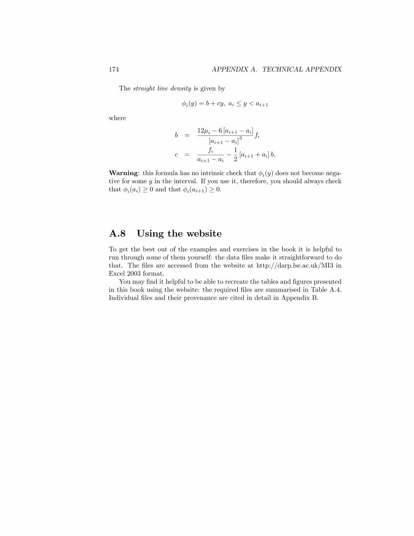
174 APPENDIX A. TECHNICAL APPENDIX
The straight line density is given by
�i(y) = b+ cy; ai � y < ai+1
where
b =12�i � 6 [ai+1 � ai]
[ai+1 � ai]3fi
c =fi
ai+1 � ai� 12[ai+1 + ai] b:
Warning: this formula has no intrinsic check that �i(y) does not become nega-tive for some y in the interval. If you use it, therefore, you should always checkthat �i(ai) � 0 and that �i(ai+1) � 0.
A.8 Using the website
To get the best out of the examples and exercises in the book it is helpful torun through some of them yourself: the data �les make it straightforward to dothat. The �les are accessed from the website at http://darp.lse.ac.uk/MI3 inExcel 2003 format.You may �nd it helpful to be able to recreate the tables and �gures presented
in this book using the website: the required �les are summarised in Table A.4.Individual �les and their provenance are cited in detail in Appendix B.
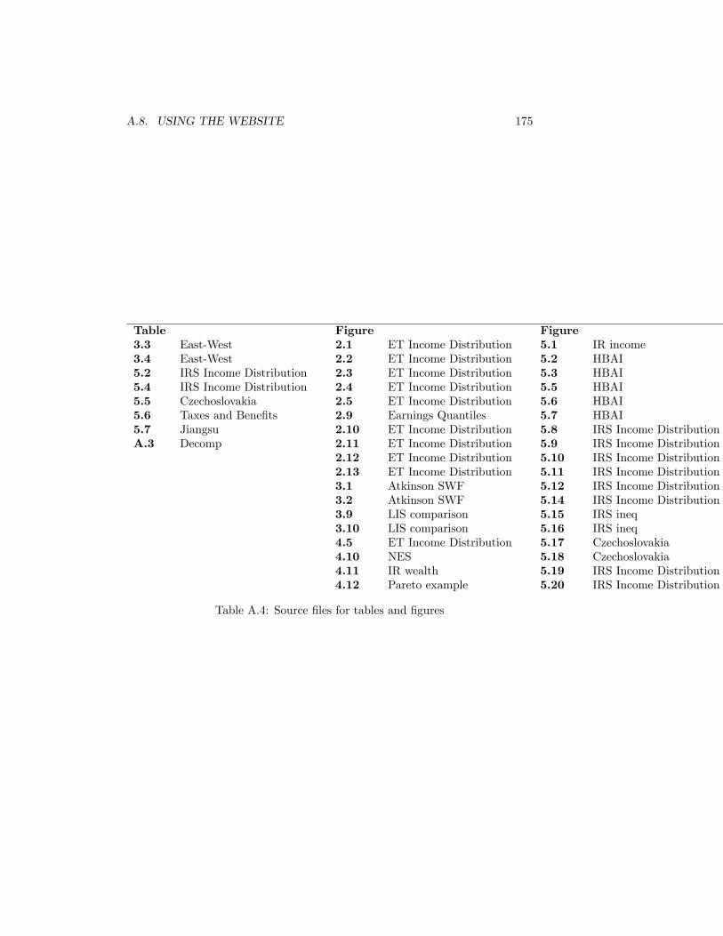
A.8. USING THE WEBSITE 175
Table Figure Figure3.3 East-West 2.1 ET Income Distribution 5.1 IR income3.4 East-West 2.2 ET Income Distribution 5.2 HBAI5.2 IRS Income Distribution 2.3 ET Income Distribution 5.3 HBAI5.4 IRS Income Distribution 2.4 ET Income Distribution 5.5 HBAI5.5 Czechoslovakia 2.5 ET Income Distribution 5.6 HBAI5.6 Taxes and Bene�ts 2.9 Earnings Quantiles 5.7 HBAI5.7 Jiangsu 2.10 ET Income Distribution 5.8 IRS Income DistributionA.3 Decomp 2.11 ET Income Distribution 5.9 IRS Income Distribution
2.12 ET Income Distribution 5.10 IRS Income Distribution2.13 ET Income Distribution 5.11 IRS Income Distribution3.1 Atkinson SWF 5.12 IRS Income Distribution3.2 Atkinson SWF 5.14 IRS Income Distribution3.9 LIS comparison 5.15 IRS ineq3.10 LIS comparison 5.16 IRS ineq4.5 ET Income Distribution 5.17 Czechoslovakia4.10 NES 5.18 Czechoslovakia4.11 IR wealth 5.19 IRS Income Distribution4.12 Pareto example 5.20 IRS Income Distribution
Table A.4: Source �les for tables and �gures

176 APPENDIX A. TECHNICAL APPENDIX
Appendix B
Notes on Sources andLiterature
These notes describe the data sets which have been used for particular examplesin each chapter, cite the sources which have been used for the discussion in thetext, and provide a guide for further reading. In addition some more reconditesupplementary points are mentioned. The arrangement follows the order of thematerial in the �ve chapters and Technical Appendix.
B.1 Chapter 1
For a general discussion of terminology and the approach to inequality you couldgo to Chapter 1 of Atkinson (1983), Cowell (2008b, 2008c) and Chapter 2 ofThurow (1975); reference may also be made to Bauer and Prest (1973). For adiscussion of the relationship between income inequality and broader aspects ofeconomic inequality see Sen (1997). For other surveys of inequality measurementissues see Jenkins and Van Kerm (2008) and for a more technical treatment,Cowell (2000), Lambert (2001).
Inequality of what?
This key question is explicitly addressed in Sen (1980, 1992). The issue of themeasurability of the income concept is taken up in a very readable contributionby Boulding (1975), as are several other basic questions about the meaning ofthe subject which were raised by the nine interpretations cited in the text (Reinand Miller 1974). For an introduction to the formal analysis of measurabilityand comparability, see Sen and Foster (1997 [Sen 1973], pp. 43-46), and perhapsthen try going on to Sen (1974) which, although harder is clearly expounded.There are several studies which use an attribute other than income or wealth,
177
178 APPENDIX B. NOTES ON SOURCES AND LITERATURE
and which provide interesting material for comparison: Jencks (1973) puts in-come inequality in the much wider context of social inequality; Addo (1976)considers international inequality in such things as school enrolment, calorieconsumption, energy consumption and numbers of physicians; Alker (1965) dis-cusses a quanti�cation of voting power; Russet (1964) relates inequality in landownership to political instability. The problem of the size of the cake dependingon the way it is cut has long been implicitly recognised (for example, in theoptimal taxation literature) but does not feature prominently in the works oninequality measurement. For a general treatment read Tobin (1970), reprintedin Phelps (1973). On this see also the Okun (1975, Chapter 4) illustration of�leaky bucket�income transfers.The issue of rescaling nominal incomes so as to make them comparable across
families or households of di¤erent types �known in the jargon as �equivalisa-tion��and its impact upon measured inequality is discussed in Coulter et al.(1992a, 1992b) �see also page 191 below. Alternative approaches to measuringinequality in the presence of household heterogeneity are discussed in Cowell(1980), Ebert (1995, 2004) Glewwe (1991) Jenkins and O�Higgins (1989), Jor-genson and Slesnick (1990). The issues of measuring inequality when the un-derlying �income�concept is something that is not cardinally measurable �forexample measuring the inequality of health status �is discussed in Abul Nagaand Yalcin (2008) Allison and Foster (2004).
Inequality measurement, justice and poverty
Although inequality is sharply distinct from mobility, inequality measures havebeen used as a simple device for characterising income mobility �after coveringthe material in Chapter 3 you may �nd it interesting to check Shorrocks (1978).The application of inequality-measurement tools to the analysis of inequality ofopportunity is addressed in Lefranc et al. (2008) and Pistolesi (2009).On the desirability of equality per se see Broome (1988). Some related ques-
tions and references are as follows: Why care about inequality?(Milanovic 2007)Does it make people unhappy? (Alesina et al. 2004) Why measure inequality?Does it matter? (Bénabou 2000, Elliott 2009, Kaplow 2005) Do inequality mea-sures really measure inequality? (Feldstein 1998)On some of the classical principles of justice and equality, see Rees (1971),
Chapter 7, Wilson (1966). The idea of basing a model of social justice uponthat of economic choice under risk is principally associated with the work ofHarsanyi (1953, 1955) �see also Bosmans and Schokkaert (2004), Amiel et al.(2009) and Cowell and Schokkaert (2001). Hochman and Rodgers (1969) discussconcern for equality as a consumption externality. A notable landmark in mod-ern thought is Rawls (1971) which, depending on the manner of interpretationof the principles of justice there expounded, implies most speci�c recommenda-tions for comparing unequal allocations. Bowen (1970) introduces the conceptof �minimum practicable inequality,�which incorporates the idea of special per-sonal merit in determining a just allocation.Stark�s (1972) approach to an equality index is based on a head-count mea-
B.2. CHAPTER 2 179
sure of poverty and is discussed in Chapter 2; Batchelder (1971 page 30) dis-cusses the �poverty gap�approach to the measurement of poverty. The intuitiverelationships between inequality and growth (or contraction) of income are setout in a novel approach by Temkin (1986) and are discussed further by Amieland Cowell (1994b) and Fields (2007). The link between a measure that cap-tures the depth of poverty and the Gini coe¢ cient of inequality (see Chapter2) was analysed in a seminal paper by Sen (1976a), which unfortunately thegeneral reader will �nd quite hard; the huge literature which ensued is surveyedby Foster (1984), Hagenaars (1986), Ravallion (1994), Seidl (1988) and Zheng(1997). The relationship between inequality and poverty measures is discussedin some particularly useful papers by Thon (1981, 1983a). An appropriate ap-proach to poverty may require a measure of economic status that is richer thanincome �see Anand and Sen (2000)
Inequality and the social structure
The question of the relationship between inequality in the whole population andinequality in subgroups of the population with reference to heterogeneity dueto age is tackled in Paglin (1975) and in Cowell (1975). The rather technicalpaper of Champernowne (1974) explores the relationship between measures ofinequality as a whole and measures that are related speci�cally to low incomes,to middle incomes, or to high incomes.
B.2 Chapter 2
The main examples here are from the tables in Economic Trends, November1987 (based on the Inland Revenue�s Survey of Personal Incomes augmentedby information from the Family Expenditure Survey), which are reproduced onthe website in the �le �ET income distribution�: the income intervals used arethose that were speci�ed in the original tables. If you open this �le you will alsosee exactly how to construct the histogram for yourself: it is well worth runningthrough this as an exercise. The reason for using these data to illustrate thebasic tools of inequality analysis is that they are based on reliable data sources,have an appropriate de�nition of income and provide a good coverage of theincome range providing some detail for both low incomes and high incomes.Unfortunately this useful series has not been maintained: we will get to theissue of what can be done with currently available data sets in Chapter 5.The example in Figure 2.9 is taken from the Annual Survey of Hours and
Earnings (formerly the New Earnings Survey) data �see �le �Earnings Quan-tiles�on the website. The reference to Plato as an early precursor of inequalitymeasurement is to be found in Saunders (1970), pp. 214-215.
Diagrams
One often �nds that technical apparatus or analytical results that have becomeassociated with some famous name were introduced years before by someone
180 APPENDIX B. NOTES ON SOURCES AND LITERATURE
else in some dusty journals, but were never popularised. So it is with Pen�sParade, set out in Pen (1974), which had been anticipated by Schutz (1951),and only rarely used since �Cf. Budd (1970). As we have seen, the Parade issimply related to the cumulative frequency distribution if you turn the piece ofpaper over once you have drawn the diagram: for more about this concept, andalso frequency distributions and histograms, consult a good statistics text suchas Berry and Lindgren (1996), Casella and Berger (2002) or Freund and Perles(2007); for an extensive empirical application of Pen�s parade see Jenkins andCowell (1994a). The log-representation of the frequency distribution is referredto by Champernowne (1973, 1974) as the �people curve.�The Lorenz curve originally appeared in Lorenz (1905). Its convex shape
(referred to on page 21) needs to be quali�ed in one very special case: wherethe mean of the thing that you are charting is itself negative � see page 167in the Technical Appendix and Amiel et al. (1996). For a formal expositionof the Lorenz curve and proof of the assertions made in the text see Levineand Singer (1970) and Gastwirth (1971). Lorenz transformations are used toanalyse the impact of income redistributive policies �see Arnold (1990), Fellman(2001) and the references in question 7 on page 37. On using a transformationof the Lorenz curve to characterise income distributions see Aaberge (2007);see Fellman (1976) and Damjanovic (2005) for general results on the e¤ect oftransformations on the Lorenz curve. Lam (1986) discusses the behaviour ofthe Lorenz curve in the presence of population growth.The relationship between the Lorenz curve and Pen�s parade is also discussed
by Alker (1970). The Lorenz curve has further been used as the basis for con-structing a segregation index (Duncan and Duncan 1955; Cortese et al. 1976).For more on the Lorenz curve see also Blitz and Brittain (1964), Crew (1982),Hainsworth (1964), Koo et al. (1981) and Riese (1987).
Inequality measures
The famous concentration ratio (Gini 1912) also has an obscure precursor.Thirty six years before Gini�s work, Helmert (1876) discussed the ordinallyequivalent measure known as Gini�s mean di¤erence � for further informationsee David (1968, 1981). Some care has to be taken when applying the Gini co-e¢ cient to indices to data where the number of individuals n is relatively small(Allison 1978, Jasso 1979): the problem is essentially whether the term n2 orn[n� 1] should appear in the denominator of the de�nition �see the TechnicalAppendix page 151. A convenient alternative form of the standard de�nition isgiven in Dorfman (1979):
G = 1� 1
�y
Z 1
0
P (y)2dy where P (y) = 1� F (y):
For an exhaustive treatment of the Gini coe¢ cient see Yitzhaki (1998).The process of rediscovering old implements left lying around in the inequality-
analyst�s toolshed continues unabated, so that often several labels and descrip-tions exist for essentially the same concept. Hence M , the relative mean de-
B.2. CHAPTER 2 181
viation, used by Schutz (1951), Dalton (1920) and Kuznets (1959), reappearsas the maximum equalisation percentage, which is exactly 2M (United NationsEconomic Commission for Europe 1957), and as the �standard average di¤er-ence�(Francis 1972). Eltetö and Frigyes (1968) produce three measures whichare closely related to M , and Addo�s �systemic inequality measure� is essen-tially a function of these related measures; see also Kondor (1971). Gini-likeinequality indices have been proposed by, Basmann and Slottje (1987), Basu(1987), Berrebi and Silber (1987), Chakravarty (1988) and Yitzhaki (1983),and generalisations and extensions of the Gini are discussed by Barrett andSalles (1995), Bossert (1990), Donaldson and Weymark (1980), Kleiber andKotz (2002), Moyes (2007), Weymark (1981) and Yaari (1988); see also Lin(1990). The Gini coe¢ cient has also been used as the basis for regression analy-sis (Schechtman and Yitzhaki 1999) and for constructing indices of relativedeprivation (Bishop et al. 1991, Chakravarty and Chakraborty 1984, Cowell2008a, Yitzhaki 1979).
The properties of the more common ad hoc inequality measures are discussedat length in Atkinson (1970, pp. 252-257; 1983, pp. 53-58), Champernowne(1974 page 805), Foster (1985), Jenkins (1991) and Sen and Foster (1997, pp.24-36). Berrebi and Silber (1987) show that for all symmetric distributionsG < 0:5: a necessary condition for G > 0:5 is that the distribution be skew tothe right. Chakravarty (2001) considers the use of the variance for the decom-position of inequality and Creedy (1977) and Foster and Ok (1999) discuss theproperties of the variance of logarithms. The use of the skewness statistic wasproposed by Young (1917); this and other statistical moments are consideredfurther by Champernowne (1974); Butler and McDonald (1989) discuss the useof incomplete moments in inequality measurement (the ordinates of the Lorenzcurve are simple examples of such incomplete moments � see the expressionson page 110). On the use of the moments of the Lorenz curve as an approachto characterising inequality see Aaberge (2000). Further details on the use ofmoments may be found in texts such as Casella and Berger (2002) and Fre-und (2003). For more on the minimal majority coe¢ cient (sometimes knownas the Dauer-Kelsay index of malapportionment) see Alker and Russet (1964),Alker (1965) and Davis (1954, pp.138-143). Some of the criticisms of Stark�shigh/low measure were originally raised in Polanyi and Wood (1974). Anothersuch practical measure with a similar �avour is Wiles (1974) semi-decile ratio:(Minimum income of top 5%)/(maximum income of bottom 5%). Like R, M ,�minimal majority�, �equal shares�, and �high/low�, this measure is insensitiveto certain transfers, notably in the middle income ranges (you can redistributeincome from a person at the sixth percentile to a person at the ninety-fourthwithout changing the semi-decile ratio). In my opinion this is a serious weak-ness, but Wiles recommended the semi-decile ratio as focusing on the essentialfeature of income inequality.
182 APPENDIX B. NOTES ON SOURCES AND LITERATURE
Rankings
Wiles and Markowski (1971) argued for a presentation of the facts about inequal-ity that captures the whole distribution, since conventional inequality measuresare a type of sophisticated average, and �the average is a very uninformativeconcept�(1971, p. 351). In this respect1 their appeal is similar in spirit to thatof Sen and Foster (1997, Chapter 3) who suggests using the Lorenz curve to rankincome distributions in a �quasi-ordering��in other words a ranking where thearrangement of some of the items is ambiguous. An alternative approach to thisnotion of ambiguity is the use of �fuzzy� inequality discussed in Basu (1987)and Ok (1995).The method of percentiles was used extensively by Lydall (1959) and Polanyi
and Wood (1974); for recent applications to trends in the earnings distributionand the structure of wages see Atkinson (2007a) and Harvey and Bernstein(2003). The formalisation of this approach as a �comparative function� wassuggested by Esberger and Malmquist (1972).
B.3 Chapter 3
The data set used for the example on page 69 is given in the �le �LIS compari-son�on the website. The arti�cial data used for the example in Tables 3.3 and3.4 are in the �le �East West.�
Social-welfare functions
The traditional view of social-welfare functions is admirably and concisely ex-pounded in Graa¤ (1957). One of the principal di¢ culties with these functions,as with the physical universe, is �where do they come from? On this tech-nically di¢ cult question, see Boadway and Bruce (1984, Chapter 5), Gaertner(2006) and Sen (1970, 1977). If you are sceptical about the practical usefulnessof SWFs you may wish to note some other areas of applied economics whereSWFs similar to those discussed in the text have been employed. They are in-troduced to derive interpersonal weights in applications of cost-bene�t analysis,and in particular into project appraisal in developing countries � see Layard(1994), Little and Mirrlees (1974, Chapter 3), Salanié (2000, Chapters 1, 2).Applications of SWF analysis include taxation design (Atkinson and Stiglitz1980, Salanié 2003, Tuomala 1990), the evaluation of the e¤ects of regionalpolicy Brown (1972, pp.81-84), the impact of tax legislation (Mera 1969), andmeasures of national income and product (Sen 1976b).As we noted when considering the basis for concern with inequality (pages
11 and 178) there is a connection between inequality and risk. This connec-tion was made explicit in Atkinson�s seminal article (Atkinson 1970) where the
1But only in this respect, since they reject the Lorenz curve as an �inept choice�, preferringto use histograms instead.
B.3. CHAPTER 3 183
analogy between risk aversion and inequality aversion was also noted. However,can we just read across from private preferences on risk to social preferenceson inequality? Amiel et al. (2008) show that the phenomenon of preferencereversals may apply to social choice amongst distributions in a manner that issimilar to that observed in personal choice amongst lotteries. However, exper-imental evidence suggests that individuals�attitude to inequality (their degreeof inequality aversion ") is sharply distinguished from their attitude to risk asre�ected in their measured risk aversion �Kroll and Davidovitz (2003), Carls-son et al. (2005). Estimates of inequality aversion across country (based ondata from the World Bank�s world development report) are discussed in Lam-bert et al. (2003). If we were to interpret U as individual utility derived fromincome we would then interpret " as the elasticity of marginal utility of incomethen one could perhaps estimate this elasticity directly from surveys of subjec-tive happiness: this is done in Layard et al. (2008). Cowell and Gardiner (2000)survey methods for estimating this elasticity and HM Treasury (2003), page 94provides a nice example of how such estimates can be used to underpin policymaking. Ebert and Welsch (2009) examine the extent to which conventionalinequality measures can be used to represent rankings of income distributionsas re�ected in survey data on subjective well-being.The dominance criterion associated with quantile ranking (or Parade rank-
ing) on page 32 and used in Theorem 1 is known as �rst-order dominance. Theconcept of second-order dominance refers to the ranking by generalised-Lorenzcurves used in Theorem 3 (the shares dominance used in Theorem 2 can beseen as a special case of second-order dominance for a set of distributions thatall have the same mean). First-order dominance, principles of social welfareand Theorem 1 are discussed in Saposnik (1981, 1983). The proofs of Theo-rems 2 and 4 using slightly more restrictive assumptions than necessary wereestablished in Atkinson (1970) who drew heavily on an analogy involving prob-ability theory; versions of these two theorems requiring weaker assumptions butrather sophisticated mathematics are found in Dasgupta et al. (1973), Kolm(1969) and Sen and Foster (1997, pp. 49-58). In fact a lot of this work wasanticipated by Hardy et al. (1934, 1952); Marshall and Olkin (1979) developthis approach and cover in detail relationships involving Lorenz curves, gener-alised Lorenz curves and concave functions (see also Arnold 1987): readers whoare happy with an undiluted mathematical presentation may �nd this the mostuseful single reference on this part of the subject.Shorrocks (1983) introduced the concept of the generalised Lorenz curve and
proved Theorem 3. As a neat logical extension of the idea Moyes (1989) showedthat if you take income and transform it by some function � (for example byusing a tax function, as in the exercises on page 37) then the generalised Lorenzordering of distributions is preserved if and only if � is concave �see also page180 above. Iritani and Kuga (1983) and Thistle (1989a, 1989b) discuss theinterrelations between the Lorenz curve, the generalised Lorenz curve and thedistribution function. A further discussion and overview of these topics is to befound in Lambert (2001).Where Lorenz curves intersect we know that unambiguous inequality com-
184 APPENDIX B. NOTES ON SOURCES AND LITERATURE
parisons cannot be made without some further restriction, such as imposing aspeci�c inequality measure. However, it is also possible to use the concept ofthird-order dominance discussed in Atkinson (2008) and Davies and Hoy (1995).For corresponding results concerning generalised Lorenz curves see Dardanoniand Lambert (1988).
SWF-based inequality measures
For the relationship of SWFs to inequality measurement, either in general form,or the speci�c type mentioned here, see Atkinson (1974, p.63; 1983, pp. 56-57), Blackorby and Donaldson (1978, 1980), Champernowne and Cowell (1998),Dagum (1990), Dahlby (1987), Schwartz and Winship (1980), Sen (1992) andSen and Foster (1997). The formal relationships between inequality and socialwelfare are discussed in Ebert (1987) and Dutta and Esteban (1992). For ageneral discussion of characterising social welfare orderings in terms of degreesof inequality aversion see Bosmans (2007a). The association of the Rawls (1971)concept of justice (where society gives priority to improving the position of theleast advantaged person) with a social-welfare function exhibiting extreme in-equality aversion is discussed in Arrow (1973), Hammond (1975), Sen (1974, pp.395-398) and Bosmans (2007b). Lambert (1980) provides an extension of theAtkinson approach using utility shares rather than income shares. Inequalitymeasures of the type �rst suggested by Dalton (1920) are further discussed byAigner and Heins (1967) and Bentzel (1970). Kolm (1976a) suggests a measurebased on an alternative to assumption 5, namely constant absolute inequalityaversion (see page 162 above), so that as we increase a person�s income y byone unit (pound, dollar, etc.) his welfare weight U 0 drops by �% where � isthe constant amount of absolute inequality aversion: this approach leads to aninequality measure which does not satisfy the principle of scale independence.He also suggests a measure generalising both this and Atkinson�s measure. Seealso Bossert and P�ngsten (1990), Yoshida (1991). The implications of usingabsolute rather than relative measures in analysing world income distributionare examined in Atkinson and Brandolini (2009a). The SWF method is inter-preted by Meade (1976, Chapter 7 and appendix) in a more blatantly utilitarianfashion; his measure of �proportionate distributional waste�is based on an es-timation of individual utility functions. Ebert (1999) suggests a decomposableinequality measure that is a kind of �inverse�of the Atkinson formula.
An ingenious way of extending dominance results to cases where individualsdi¤er in their needs as well as their incomes is the concept known as sequen-tial dominance Atkinson and Bourguignon (1982, 1987). Further discussion ofmultidimensional aspects of inequality are to be found in Diez et al. (2007),Maasoumi (1986, 1989), Rietveld (1990), Savaglio (2006) and Weymark (2006);multidimensional inequality indices are discussed by Tsui (1995).
B.3. CHAPTER 3 185
Inequality and information theory
The types of permissible �distance� function, and their relationship with in-equality are discussed in Cowell and Kuga (1981); Love and Wolfson (1976)refer to a similar concept as the �strength-of-transfer e¤ect�. The special rela-tionship of the Her�ndahl index and the Theil index to the strong principle oftransfers was �rst examined in Kuga (1973). Krishnan (1981) (see also replyby Allison 1981) discusses the use of the Theil index as a measure of inequal-ity interpreted in terms of average distance. Kuga (1980) shows the empiricalsimilarities of the Theil index and the Gini coe¢ cient, using simulations.The Her�ndahl (1950) index (closely related to c2, or to Francis�standard
average square di¤erence) was originally suggested as a measure of concentrationof individual �rms �see Rosenbluth (1955). Several other inequality measurescan be used in this way, notably other members of the E� family. The variablecorresponding to income y may then be taken to be a �rm�s sales. However,one needs to be careful about this analogy since inequality among persons andconcentration among �rms are rather di¤erent concepts in several importantways: (i) the de�nition of a �rm is often unclear, particularly for small produc-tion units; (ii) in measuring concentration we may not be very worried aboutthe presence of tiny sales shares of many small �rms, whereas in measuring in-equality we may be considerably perturbed by tiny incomes received by a lot ofpeople �see Hannah and Kay (1977). The relationship between the generalisedentropy measures and the Lorenz curves is examined further in Rohde (2008)and the problem of capturing Lorenz orderings by a small number of inequalitymeasures is considered by Shorrocks and Slottje (2002).A reworking of the information theory analogy leads us to a closely related
class of measures that satisfy the strong principle of transfers, but where theaverage of the distance of actual incomes from inequality is found by usingpopulation shares rather than income shares as weights, thus:
1
�
nXi=1
1
n
�h (si)� h
�1
n
���compare equation (3.6) on page 57. The special case � = 0 which becomesPn
i=1 log(�y=yi)=n (the MLD index) was already discussed in Theil (1967, Chap-ter 4, page 126 and appendix). An ordinally equivalent variant of Theil�s indexis used in Marfels (1971); see also Gehrig (1988). Jasso (1980) suggests that anappropriate measure of justice evaluation for an individual is log(actual share /just share). From this it is easy to see that you will get a generalised entropymeasure with parameter � = 0 (equivalently Atkinson index with " = 1).
Building an inequality measure
The social value judgements implied by the use of the various ad hoc inequalitymeasures in Chapters 2 and 3 are analysed in Kondor (1975) who extends thediscussion in the works of Atkinson, Champernowne and Sen cited in the notesto Chapter 2. The question of what happens to inequality measures when
186 APPENDIX B. NOTES ON SOURCES AND LITERATURE
all incomes are increased or when the population is replicated or merged withanother population is discussed in Aboudi et al. (2009), Frosini (1985), Eichhornand Gehrig (1982), Kolm (1976a, 1976b) and Salas (1998). Shorrocks and Foster(1987) examine the issue of an inequality measure�s sensitivity to transfers indi¤erent parts of the distribution and Barrett and Salles (1998) discuss classesof inequality measures characterised by their behaviour under income transfers;Lambert and Lanza (2006) analyse the e¤ect on inequality of changing isolatedincomes. The Atkinson and generalised entropy families are examples of theapplication of the concept of the quasi-linear mean, which is discussed in Hardyet al. (1934, 1952) and Chew (1983).Distributional principles that can be applied when households are not ho-
mogeneous are discussed in Ebert (2007) and Shorrocks (2004). The axiomaticapproach to inequality measurement discussed on page 65 is not of course re-stricted to the generalised entropy family; with a suitable choice of axiom theapproach can be extended to pretty well any inequality measure you like: for ex-ample see Thon�s (1982) axiomatisation of the Gini coe¢ cient, or Foster (1983)on the Theil index. The validity of standard axioms when viewed in the lightof people�s perceptions of inequality is examined in Amiel and Cowell (1992,1994a, 1999) and Cowell (1985a); for a discussion and survey of this type ofapproach see Amiel (1999) and Kampelmann (2009). The problematic caseshighlighted in the examples on page 37 and 64 are based on Cowell (1988a).Ebert (1988) discusses the principles on which a generalised type of the relativemean deviation may be based and Ebert (2009) addresses ways of axiomatis-ing inequality that will be consistent to with the apparently heterodox viewsillustrated in Question 4 on page 73.The normative signi�cance of decomposition is addressed by Kanbur (2006).
Examples of approaches to inequality measurement that explicitly use criteriathat may con�ict with decomposability include basing social welfare on incomesatisfaction in terms of ranks in the distribution (Hempenius 1984), the use ofincome gaps (Preston 2007), the use of reference incomes to capture the ideaof individual �complaints�about income distribution (Cowell and Ebert 2004,Devooght 2003, Temkin 1993) �see also the discussion on page 195.
B.4 Chapter 4
The idea of a model
For an excellent coverage of the use of functional forms in modelling incomedistributions see Kleiber and Kotz (2003).
The lognormal distribution
Most texts on introductory statistical theory give a good account of the normaldistribution �for example Berry and Lindgren (1996), Casella and Berger (2002)or Freund and Perles (2007). The standard reference on the lognormal and its
B.4. CHAPTER 4 187
properties (Aitchison and Brown 1957) also contains a succinct account of asimple type of random process theory of income development. A summaryof several such theories can be found in Bronfenbrenner (1971) and in Brown(1976). On some of the properties of the lognormal Lorenz curve, see alsoAitchison and Brown (1954).
The Pareto distribution
An excellent introduction to Pareto�s law is provided by Persky (1992). Pareto�soriginal work can be consulted in Pareto (1896, 1965, 2001) or in Pareto (1972),which deals in passing with some of Pareto�s late views on the law of incomedistribution; the development of Pareto�s thought on inequality is discussed inMaccabelli (2009). Tawney (1964) argues forcefully against the strict interpre-tation of Pareto�s law: �It implies a misunderstanding of the nature of economiclaws in general, and of Pareto�s laws in particular, at which no one, it is proba-ble, would have been more amused than Pareto himself, and which, indeed, heexpressly repudiated in a subsequent work. It is to believe in economic Funda-mentalism, with the New Testament left out, and the Books of Leviticus andDeuteronomy in�ated to unconscionable proportions by the addition of new andappalling chapters. It is to dance naked, and roll on the ground, and cut oneselfwith knives, in honour of the mysteries of Mumbo Jumbo.�However, I do not�nd his assertion of Pareto�s recantation convincing �see Pareto (1972); see alsoPigou (1952, pp.650 ¤.). Oversimpli�ed interpretations of the law have persisted�Adams (1976) suggested a �golden section�value of � = 2=[
p5� 1] as a cure
for in�ation. Van der Wijk�s (1939) law is partially discussed in Pen (1974,Chapter 6); in a sense it is a mirror image of the Bonferroni index (Bonferroni1930) which is formed from an average of �lower averages��see Chakravarty(2007). Several of the other results in the text are formally proved in Chipman(1974). Nicholson (1969, pp. 286-292) and Bowman (1945) give a simple ac-count of the use of the Pareto diagram. The discussion of a random processmodel leading to a Pareto distribution is presented in Champernowne (1953,1973) and the non-technical reader will �nd a simple summary in Pen (19711974). The Pareto distribution as an equilibrium distribution of a wealth modelis treated in Wold and Whittle (1957) and Champernowne and Cowell (1998),Chapter 10. A recent overview of Pareto-type distributions in economics and�nance is provided by Gabaix (2008).
How good are the functional forms?
The example of earnings displayed on page 92 can be reproduced from �le �NES�on the website; the income example of page 86 is taken from the website �le�ET income distribution� again, and the wealth example on page 93 is basedon �le �IR wealth.� Evidence on the suitability of the Pareto and lognormaldistributions as approximations to actual distributions of earnings and of incomecan be found in the Royal Commission on the Distribution of Income and Wealth(1975, Appendix C; 1976, Appendix E).
188 APPENDIX B. NOTES ON SOURCES AND LITERATURE
In discussing the structure of wages in Copenhagen in 1953 Bjerke (1970)showed that the more homogenous the occupation, the more likely it wouldbe that the distribution of earnings within it was lognormal. Weiss (1972)shows the satisfactory nature of the hypothesis of lognormality for graduatescientists� earnings in di¤erent areas of employment � particularly for thosewho were receiving more than $10 000 a year. Hill (1959) shows that mergingnormal distributions with di¤erent variances leads to �leptokurtosis�(more of thepopulation in the �tails�than expected from a normal distribution) �a typicalfeature of the distribution of the logarithm of income. Other useful referenceson the lognormal distribution in practice are Fase (1970), Takahashi (1959),Thatcher (1968). Evidence for lognormality is discussed in the case of India(Rajaraman 1975), Kenya (Kmietowicz and Webley 1975), Iraq (Kmietowicz1984) and China (Kmietowicz and Ding 1993). Kmietowicz (1984) extends theidea of lognormality of the income distribution to bivariate lognormality of thejoint distribution of income and household size.Atkinson (1975) and Soltow (1975) produce evidence on the Pareto distri-
bution and the distribution of wealth in the UK and the USA of the 1860�srespectively. Klass et al. (2006) do this using the Forbes 400; Clementi andGallegati (2005) examine Pareto�s law for Germany, the UK and the USA. Forfurther evidence on the variability of Pareto�s � in the USA, see Johnson (1937),a cautious supporter of Pareto. The Paretian property of the tail of the wealthdistribution is also demonstrated admirably by the Swedish data examined bySteindl (1965) where � is about 1.5 to 1.7.Some of the less orthodox applications of the Pareto curve are associated with
�Zipf�s law� (Zipf 1949) which has been fruitfully applied to the distributionof city size (Nitsch 2005). Harold T. Davis, who has become famous for histheory of the French Revolution in terms of the value of Pareto�s � under LouisXVI, produces further evidence on the Pareto law in terms of the distributionof wealth in the pre-Civil War southern states (wealth measured in terms ofnumber of slaves) and of the distribution of income in England under William theConqueror �see Davis (1954). For the latter example (based on the DomesdayBook, 1086) the �t is surprisingly good, even though income is measured in�acres��i.e. that area of land which produces 72 bushels of wheat per annum.The population covered includes Cotters, Serfs, Villeins, Sokemen, Freemen,Tenants, Lords and Nobles, Abbots, Bishops, the Bishop of Bayeux, the Countof Mortain, and of course King William himself.However, Davis�s (1941) interpretation of these and other intrinsically inter-
esting historical excursions as evidence for a �mathematical theory of history�seems mildly bizarre: supposedly if � is too low or too high a revolution (fromthe left or the right, respectively) is induced. Although there is clearly a con-nection between extreme economic inequality and social unrest, seeking themainspring of the development of civilisation in the slope of a line on a double-log graph does not appear to be a rewarding or convincing exercise. There is asimilar danger in misinterpreting a dynamic model such as of Champernowne(1953), in which a given pattern of social mobility always produces, eventually,a unique Pareto distribution, independent of the income distribution originally
B.4. CHAPTER 4 189
prevailing. Bernadelli (1944) postulates that a revolution having redistributionas an aim will prove futile because of such a mathematical process. Finding thelogical and factual holes in this argument is left as an exercise for you.
Other distributions
Finally, a mention of other functional forms that have been claimed to �t ob-served distributions more or less satisfactorily (see the Technical Appendix page156). Some of these are generalisations of the lognormal or Pareto forms, such asthe three-parameter lognormal, (Metcalf 1969), or the generalised Pareto-Levylaw, which attempts to take account of the lower tail (Arnold 1983, Mandel-brot 1960). Indeed, the formula we have described as the Pareto distributionwas only one of many functions suggested by Pareto himself; it may thus bemore accurately described as a �Pareto type I� distribution (Hayakawa 1951,Quandt 1966). Champernowne (1952) provides a functional form which is closeto the Pareto in the upper tail and which �ts income distributions quite well;some technical details on this are discussed in Harrison (1974), with empiricalevidence in Thatcher (1968) � see also Harrison (1979, 1981), Sarabia et al.(1999).
Other suggestions are Beta distribution (Slottje 1984, Thurow 1970), theGamma distribution (Salem and Mount 1974, McDonald and Jensen 1979),the sech2-distribution, which is a special case of the Champernowne (1952)distribution (Fisk 1961), and the Yule distribution (Simon 1955, 1957; Simonand Bonini 1958); see also Campano (1987) and Ortega et al. (1991). Evanset al. (1993) and Kleiber and Kotz (2003) provide a very useful summary of themathematical properties of many of the above. The Singh and Maddala (1976)distribution is discussed further in Cramer (1978), Cronin (1979), McDonaldand Ransom (1979), Klonner (2000) (�rst-order dominance) and Wil�ing andKrämer (1993) (Lorenz curves); Cf also the closely related model by Dagum(1977). A generalised form of the Gamma distribution has been used by Esteban(1986), Kloek and Van Dijk (1978) and Taille (1981). An overview of severalof these forms and their interrelationships is given in McDonald (1984) as partof his discussion of the Generalised Beta distribution of the second kind; onthis distribution see also Bordley et al. (1996), Jenkins (2009), Majumder andChakravarty (1990), McDonald and Mantrala (1995), Parker (1999), Sarabiaet al. (2002), Wil�ing (1996) and for an implementation with Chinese datasee Chotikapanich et al. (2007). Alternative approaches to parameterising theLorenz curve are discussed in Basmann et al. (1990, 1991), and Kakwani andPodder (1973).
Yet other distributions include those based on the exponential distributionare considered in Jasso and Kotz (2007). Some of the Lorenz properties notedfor the lognormal and for the Pareto hold for more general functional forms �see Arnold et al. (1987) and Taguchi (1968).
190 APPENDIX B. NOTES ON SOURCES AND LITERATURE
B.5 Chapter 5
The data
The UK data used for Figure 5.1 are from Inland Revenue Statistics (see �le�IR income�on the website), and the US data in Table 5.1 from Internal Rev-enue Service, Statistics of Income: Individual Tax Returns (see �le �IRS IncomeDistribution�). The UK data used for Figures 5.2-5.7 are taken from the House-holds Below Average Income data set (HBAI), which is now the principal datasource for UK income distribution; summary charts and results are publishedin Department of Work and Pensions (2009).For a general introduction to the problem of specifying an income or wealth
variable, see Atkinson (1983). The quality of the administrative data on per-sonal incomes �derived from tax agencies or similar o¢ cial sources �dependscrucially on the type of tax administration and government statistical servicefor the country in question. On the one hand extremely comprehensive anddetailed information about income and wealth (including cross-classi�cationsof these two) is provided, for example, by the Swedish Central Statistical Bu-reau, on the basis of tax returns. On the other, one must overcome almostinsuperable di¢ culties where the data presentation is messy, incomplete or de-signedly misleading. An excellent example of the e¤ort required here is providedby the geometric detective work of Wiles and Markowski (1971) and Wiles(1974) in handling Soviet earnings distribution data. Fortunately for the re-search worker, some government statistical services modify the raw tax data soas to improve the concept of income and to represent low incomes more satis-factorily. Stark (1972) gives a detailed account of the signi�cance of re�nementsin the concepts of income using the UK data; for an exhaustive description ofthese data and their compilation see Stark in Atkinson et al. (1978) and for aquick summary, Royal Commission on the Distribution of Income and Wealth(1975, Appendices F and H). For a discussion of the application of tax datato the analysis of top incomes see Atkinson (2007b). As for survey data onincomes the HBAI in the UK draws on the Family Resources Survey and Fam-ily Expenditure Survey � see Frosztega (2000) for a detailed consideration ofthe underlying income concept: UK data sets are available from the UK DataArchive http://www.data-archive.ac.uk. Summary charts and results for HBAIare published in Department of Work and Pensions (2009) and Brewer et al.(2008) provide a useful critique of this source. On the widely used the CurrentPopulation Survey (CPS) data (see question 3 in Chapter 2) in the USA seeBurkhauser et al. (2004) and Welniak (2003). A general overview of inequalityin the USA is provided in Bryan and Martinez (2008), Reynolds (2006) andRyscavage (1999). Two classic references on US data and the quality of samplesurveys in particular see Budd and Radner (1975) and (Ferber et al. 1969) .Since publication of the �rst edition of this book large comprehensive datasetsof individual incomes have become much more readily available; it is impossibleto do justice to them. One that deserves attention from the student of in-equality are the early example based on data from the Internal Revenue Service
B.5. CHAPTER 5 191
and Survey of Economic Opportunity discussed in Okner (1972, 1975); an ex-tremely useful source of internationally comparable micro data in incomes (andmuch else) is the Luxembourg Income Study (http://www.lis-project.org). Anearly and comprehensive source of US longitudinal data is the Panel Study ofIncome Dynamics (http://psidonline.isr.umich.edu/) described in Hill (1992);more recent European examples of longitudinal data are the British House-hold Panel Survey (http://www.iser.essex.ac.uk/survey/bhps) and the GermanSocio-Economic Panel (http://www.diw-berlin.de/de/soep). Wealth data in theUK are considered in detail in Atkinson and Harrison (1978) and an importantresource for international comparisons of wealth distributions is provided by theLuxembourg Wealth Study (Sierminska et al. 2006), OECD (2008) Chapter 10.A good statement of principles concerning the income concept is provided
by the Canberra Group (2001) report. Several writers have tried to combinetheoretical sophistication with empirical ingenuity to extend income beyond theconventional de�nition. Notable among these are the income-cum-wealth analy-sis of Weisbrod and Hansen (1968), and the discussion by Morgan et al. (1962)of the inclusion of the value of leisure time as an income component. An im-portant development for international comparisons is the Human DevelopmentIndex which has income as just one component (Anand and Sen 2000); Fleur-baey and Gaulier (2009) in similar spirit propose a measure of living standardsfor international comparisons based on GDP per capita adjusted for personaland social characteristics including inequality; perhaps unsurprisingly the rank-ing of countries by this measure di¤ers substantially from the conventional GDPranking. Goodman and Old�eld (2004) contrast income inequality and expen-diture inequality in the UK context. Stevenson and Wolfers (2008) examine theway inequality in happiness has changed in the USA.In Morgan (1962), Morgan et al. (1962) and Prest and Stark (1967) the e¤ect
of family grouping on measured inequality is considered. For a fuller discussionof making allowance for income sharing within families and the resulting prob-lem of constructing �adult equivalence�scales, consult Abel-Smith and Bagley(1970); the internationally standard pragmatic approach to equivalisation is theOECD scale (see for example Atkinson et al. 1995) although many UK stud-ies use a scale based on McClements (1977); the idea that equivalence scalesare revealed by community expenditures is examined in Olken (2005). The re-lationship between equivalence scales and measured inequality is examined inBuhmann et al. (1988), Coulter et al. (1992b) and Jenkins and Cowell (1994b):for a survey see Coulter et al. (1992a). The fact that averaging incomes overlonger periods reduces the resulting inequality statistics emerges convincinglyfrom the work of Hanna et al. (1948) and Benus and Morgan (1975). Thekey reference on the theoretical and empirical importance of price changes onmeasured inequality is Muellbauer (1974); see also Crawford and Smith (2002),Hobijn and Lagakos (2005), Slottje (1987). A further complication which needsto be noted from Metcalf (1969) is that the way in which price changes a¤ectlow-income households may depend on household composition; whether thereis a male bread-winner present is particularly important. On the e¤ect of non-response on income distribution and inequality refer to Korinek et al. (2006)
192 APPENDIX B. NOTES ON SOURCES AND LITERATURE
International comparisons of data sets on inequality and poverty are pro-vided by Ferreira and Ravallion (2009); an early treatment of the problems ofinternational comparison of data is found in Kuznets (1963, 1966) and Atkinsonand Brandolini (2009b) provide an excellent general introduction to issues ofdata quality. Appropriate price adjustments to incomes can be especially prob-lematic when making international comparisons. A standard approach is to usean index of Purchasing Power Parity (PPP) rather than converting incomes atnominal exchange rates. The issues involved in constructing PPP are treated inHeston et al. (2001); the method of imputation of PPP can have a substantialimpact on estimates of between-country inequality and hence on the picture ofglobal inequality; the topic is treated exhaustively in Anand and Segal (2008),Kravis et al. (1978a, 1978b) and Summers and Heston (1988, 1991). The issueof international comparability of income distribution data is one of the mainreasons for the existence of the Luxembourg Income Study: see Smeeding et al.(1990) for an introduction and a selection of international comparative stud-ies; Lorenz comparisons derived from this data source are in the website �le�LIS comparison.� On the use of data in OECD countries see Atkinson andBrandolini (2001) and on international comparisons of earnings and income in-equality refer to Gottschalk and Smeeding (1997). Atkinson and Micklewright(1992) compare the income distributions in Eastern European economies in theprocess of transition. Other important international sources for studying in-equality are Deininger and Squire (1996) and also UNU-WIDER (2005) whichprovides Gini indices drawn from a large number of national sources.
Beckerman and Bacon (1970) provide a novel approach to the measurementof world (i.e. inter-country) inequality by constructing their own index of �in-come per head�for each country from the consumption of certain key commodi-ties. Becker et al. (2005) examine the e¤ect on trends in world inequality oftrying to take into account people�s quality of life.
Computation of the inequality measures
For detail on computation of point estimates of inequality go to the TechnicalAppendix. For an excellent general text on empirical methods including com-putation of inequality measures and other welfare indicators see Deaton (1997).For a discussion of how to adapt standard methodology to estimation problemsin small areas with few observations see Tarozzi and Deaton (2009).
Decomposition techniques have been widely used to analyse spatial inequal-ity (Shorrocks and Wan 2005) including China (Yu et al. 2007) and Euroland(Beblo and Knaus 2001) and for the world as a whole (Novotný 2007). For asystematic analysis of world inequality using (fully decomposable) generalisedentropy indices see Berry et al. (1983a, 1983b), Bourguignon and Morrisson(2002), Sala-i-Martin (2006), Ram (1979, 1984, 1987, 1992), Theil (1979b, 1989);Milanovic and Yitzhaki (2002) use the (not fully decomposable) Gini coe¢ cient.
B.5. CHAPTER 5 193
Appraising the calculations
An overview of many of the statistical issues is to be found in Cowell (1999) andNygård and Sandström (1981, 1985). If you are working with data presentedin the conventional grouped form, then the key reference on the computationof the bounds JL, JU is Gastwirth (1975). Now in addition to the boundson inequality measures that we considered in the text Gastwirth (1975) showsthat if one may assume �decreasing density�over a particular income interval(i.e. the frequency curve is sloping downwards to the right in the given incomebracket) then one can calculate bounds J 0L, J
0U that are sharper � i.e. the
bounds J 0L, J0U lie within the range of inequality values (JL, JU ) which we
computed: the use of these re�ned bounds leaves the qualitative conclusionsunchanged, though the proportional gap is reduced a little. The problem of�nding such bounds is considered further in Cowell (1991). The special case ofthe Gini coe¢ cient is treated in Gastwirth (1972), and McDonald and Ransom(1981); the properties of bounds for grouped data are further discussed inGastwirth et al. (1986); Mehran (1975) shows that you can work out boundson G simply from a set of sample observations on the Lorenz curve withouthaving to know either mean income or the interval boundaries a1; a2; :::; ak+1and Hagerbaumer (1977) suggests the upper bound of the Gini coe¢ cient as aninequality measure in its own right. In Gastwirth (1972, 1975) there are alsosome re�ned procedures for taking into account the open-ended interval formingthe top income bracket �an awkward problem if the total amount of incomein this interval is unknown. Ogwang (2003) discusses the problem of puttingbounds on Gini coe¢ cient when data are sparse. As an alternative to themethods discussed in the Technical Appendix (using the Pareto interpolation,or �tting Paretian density functions), the procedure for interpolating on Lorenzcurves introduced by Gastwirth and Glauberman (1976) works quite well.Cowell and Mehta (1982) investigate a variety of interpolation methods for
grouped data and also investigate the robustness of inequality estimates underalternative grouping schemes. Aghevli and Mehran (1981) address the problemof optimal choice of the income interval boundaries used in grouping by consid-ering the set of values fa1; a2; :::; akg which will minimise the Gini coe¢ cient;Davies and Shorrocks (1989) re�ne the technique for larger data sets.For general information on the concept of the standard error see Berry and
Lindgren (1996) or Casella and Berger (2002). On the sampling properties ofinequality indices generally see Victoria-Feser (1999). Formulas for standarderrors of speci�c inequality measures can be found in the following references:Kendall et al. (1994), sec 10.5 [relative mean deviation, coe¢ cient of variation],David (1968, 1981), Nair (1936) [Gini�s mean di¤erence], Gastwirth (1974a)[relative mean deviation], Aitchison and Brown (1957 p.39) [variance of loga-rithms]. For more detailed analysis of the Gini coe¢ cient see Davidson (2009),Deltas (2003), Gastwirth et al. (1986), Giles (2004), Glasser (1962), Lomnicki(1952), Modarres and Gastwirth (2006), Nygård and Sandström (1989), Ogwang(2000,2004) and Sandström et al. (1985, 1988). Allison (1978) discusses issuesof estimation and testing based on microdata using the Gini coe¢ cient, coe¢ -
194 APPENDIX B. NOTES ON SOURCES AND LITERATURE
cient of variation and Theil index. The statistical properties of the generalisedentropy and related indices are discussed by Cowell (1989) and Thistle (1990).A thorough treatment of statistical testing of Lorenz curves is to be found inBeach and Davidson (1983), Beach and Kaliski (1986) Beach and Richmond(1985) and Davidson and Duclos (2000); for generalised Lorenz estimation referto Bishop, Chakraborti, and Thistle (1989), and Bishop, Formby, and This-tle (1989). See also Hasegawa and Kozumi (2003) for a Bayesian approach toLorenz estimation and Schluter and Trede (2002) for problems of inference con-cerning the tails of Lorenz curves. For a treatment of the problem of estimationwith complex survey design go to Biewen and Jenkins (2006), Cowell and Jenk-ins (2003), Binder and Kovacevic (1995), Bhattacharya (2007) and Kovacevicand Binder (1997). Cowell and Victoria-Feser (2003) treat the problem esti-mation and inference when the distribution may be censored or truncated andCowell and Victoria-Feser (2007, 2008) discuss the use of a Pareto tail in a�semi-parametric�approach to estimation from individual data. The e¤ect oftruncation bias on inequality judgments is also discussed in Fichtenbaum andShahidi (1988) and Bishop et al. (1994); the issue of whether �top-coding�(censoring) of the CPS data makes a di¤erence to the estimated trends in USincome inequality is analysed in Burkhauser et al. (2008). So-called �bootstrap�or resampling methods are dealt with by Biewen (2002), Davidson and Flachaire(2007) and Tarozzi and Deaton (2009) �see also Davison and Hinkley (1996).For an interesting practical example of the problem of ranking distributions byinequality when you take into account sampling error see Horrace et al. (2008).On the robustness properties of measures in the presence of contamination
or outliers see Cowell and Victoria-Feser (1996, 2002, 2006) and for the way in-equality measures respond to extreme values go to Cowell and Flachaire (2007).Chesher and Schluter (2002) discuss more generally the way measurement errorsa¤ect the comparison of income distributions in welfare terms.
Fitting functional forms
Refer to Chotikapanich and Gri¢ ths (2005) on the problem of how to choose afunctional form for your data and to Maddala and Singh (1977) for a generaldiscussion of estimation problems in �tting functional forms. Ogwang and Rao(2000) use hybrid Lorenz curves as method of �t. If you want to estimatelognormal curves from grouped or ungrouped data, you should refer to Aitchisonand Brown (1957 pp. 38-43, 51-54) �rst. Baxter (1980), Likes (1969), Malik(1970) and Quandt (1966) deal with the estimation of Pareto�s � for ungroupeddata. Now the ordinary least squares method, discussed by Quandt, despiteits simplicity has some undesirable statistical properties, as explained in Aignerand Goldberger (1970). In the latter paper you will �nd a discussion of thedi¢ cult problem of providing maximum likelihood estimates for � from groupeddata. The fact that in estimating a Pareto curve a curve is �tted to cumulativeseries which may provide a misleadingly good �t was noted in Johnson (1937),while Champernowne (1956) provided the warning about uncritical use of thecorrelation coe¢ cient as a criterion of suitability of �t. The suggestion of using
B.6. TECHNICAL APPENDIX 195
inequality measures as an alternative basis for testing goodness-of-�t was �rstput forward by Gastwirth and Smith (1972), where they test the hypothesis oflognormality for United States IRS data; see also Gail and Gastwirth (1978b,1978a). To test for lognormality one may examine whether the skewness and thekurtosis (�peakedness�) of the observed distribution of the logarithms of incomesare signi�cantly di¤erent from those of a normal distribution; for details consultKendall et al. (1999). Hu (1995) discusses the estimation of Gini from groupeddata using a variety of speci�c functional forms.
B.6 Technical Appendix
For a general technical introduction see Duclos and Araar (2006) and Cowell(2000); functional forms for distributions are discussed in Kleiber and Kotz(2003) and Evans et al. (1993).The formulas in the Technical Appendix for the decomposition of inequality
measures are standard �see Bourguignon (1979), Cowell (1980) , Das and Parikh(1981, 1982) and Shorrocks (1980).For a characterisation of some general results in decomposition see Bosmans
and Cowell (2009), Chakravarty and Tyagarupananda (1998, 2000), Cowell(2006), Foster and Shneyerov (1999), Kakamu and Fukushige (2009), Toyoda(1980), Shorrocks (1984, 1988) and Zheng (2007). Establishing the main resultstypically requires the use of functional equations techniques, on which see Aczél(1966). For applications of the decomposition technique see the references onspatial and world inequality in Chapter 5 (page 192) and also Anand (1983),Borooah et al. (1991), Ching (1991), Cowell (1984, 1985b), Frosini (1989),Glewwe (1986), Mookherjee and Shorrocks (1982), Paul (1999)..Decomposition by income components is discussed by Satchell (1978), Shorrocks
(1982) and Theil (1979a). Applications to Australia are to be found in Paul(2004) to New Zealand in Podder and Chatterjee (2002) and to UK in Jenkins(1995). The issues underlying an application of the Shapley value to decomposi-tion analysis are examined in Sastre and Trannoy (2002). The use of partitionsinto subgroups as a method of �explaining�the contributory factors to inequalityis dealt with in Cowell and Jenkins (1995) and Elbers et al. (2008). Alternativepragmatic approaches to accounting for changes in inequality are provided byBourguignon et al. (2008), Morduch and Sicular (2002), Fields (2003) and Jenk-ins and Van Kerm (2005); Cowell and Fiorio (2009) reconcile these alternativeswith conventional decomposition analysis.The relationship between decomposition of inequality and the measurement
of poverty is examined in Cowell (1988b). As noted in Chapter 3 the decomposi-tion of the Gini coe¢ cient presents serious problems of interpretation. However,Pyatt (1976) tackles this by �decomposing� the Gini coe¢ cient into a com-ponent that represents within-group inequality, one that gives between-groupinequality, and one that depends on the extent to which income distributionsin di¤erent groups overlap one another. The properties of the Gini when �de-composed� in this way are further discussed by Lambert and Aronson (1993),
196 APPENDIX B. NOTES ON SOURCES AND LITERATURE
Lerman and Yitzhaki (1984, 1989), Yitzhaki and Lerman (1991) and Sastryand Kelkar (1994). Braulke (1983) examines the Gini decomposition on the as-sumption that within-group distributions are Paretian. Silber (1989) discussesthe decomposition of the Gini coe¢ cient by subgroups of the population (forthe case of non-overlapping partitions) and by income components.The data in Table A.3 is based on Howes and Lanjouw (1994) and Hussain
et al. (1994). For recent decomposition analysis of China see Kanbur andZhang (1999, 2005), Lin et al. (2008) and Sicular et al. (2007).
Bibliography
Aaberge, R. (2000). Characterizations of Lorenz curves and income distribu-tions. Social Choice and Welfare 17, 639�653.
Aaberge, R. (2007). Gini�s nuclear family. Journal of Economic Inequality 5,305�322.
Abel-Smith, B. and C. Bagley (1970). The problem of establishing equivalentstandards of living for families of di¤erent composition. In P. Townsend(Ed.), The Concept of Poverty. London: Heinemann.
Aboudi, R., D. Thon, and S. W. Wallace (2009). Inequality comparisons whenthe populations di¤er in size. Journal Of Economic Inequality .
Abul Naga, R. H. and T. Yalcin (2008). Inequality measurement for orderedresponse health data. Journal of Health Economics 27, 1614�1625.
Aczél, J. (1966). Lectures on Functional Equations and their Applications.Number 9 in Mathematics in Science and Engineering. New York: Acad-emic Press.
Adams, K. (1976). Pareto�s answer to in�ation. New Scientist 71, 534�537.
Addo, H. (1976). Trends in international value-inequality 1969-1970: an em-pirical study. Journal of Peace Research 13, 13�34.
Aghevli, B. B. and F. Mehran (1981). Optimal grouping of income distributiondata. Journal of the American Statistical Association 76, 22�26.
Aigner, D. J. and A. S. Goldberger (1970). Estimation of Pareto�s law fromgrouped observations. Journal of the American Statistical Association 65,712�723.
Aigner, D. J. and A. J. Heins (1967). A social welfare view of the measurementof income equality. Review of Income and Wealth 13 (3), 12�25.
Aitchison, J. and J. A. C. Brown (1954). On the criteria for descriptions ofincome distribution. Metroeconomica 6, 88�107.
Aitchison, J. and J. A. C. Brown (1957). The Lognormal Distribution. London:Cambridge University Press.
Alesina, A., R. Di Tella, and R. MacCulloch (2004). Inequality and happiness:are Europeans and Americans di¤erent? Journal of Public Economics 88,2009�2042.
197
198 BIBLIOGRAPHY
Alker, H. R. (1965). Mathematics and Politics. New York: Macmillan.
Alker, H. R. J. (1970). Measuring inequality. In E. R. Tufte (Ed.), The Quan-titative Analysis of Social Problems. Reading, Massachusetts: Addison-Wesley.
Alker, H. R. J. and B. Russet (1964). On measuring inequality. BehavioralScience 9, 207�218.
Allison, P. D. (1978). Measures of inequality. American Sociological Re-view 43, 865�880.
Allison, P. D. (1981). Inequality measures for nominal data. American Soci-ological Review 46, 371�372. Reply to Krishnan.
Allison, R. A. and J. E. Foster (2004). Measuring health inequality usingqualitative data. Journal of Health Economics 23, 505½U552.
Amiel, Y. (1999). The subjective approach to the measurement of income in-equality. In J. Silber (Ed.), Handbook on Income Inequality Measurement.Dewenter: Kluwer.
Amiel, Y. and F. A. Cowell (1992). Measurement of income inequality: Ex-perimental test by questionnaire. Journal of Public Economics 47, 3�26.
Amiel, Y. and F. A. Cowell (1994a). Income inequality and social welfare. InJ. Creedy (Ed.), Taxation, Poverty and Income Distribution, pp. 193�219.Edward Elgar.
Amiel, Y. and F. A. Cowell (1994b). Inequality changes and income growth.In W. Eichhorn (Ed.), Models and measurement of welfare and inequality,pp. 3�26. Berlin, Heidelberg: Springer-Verlag.
Amiel, Y. and F. A. Cowell (1998). Distributional orderings and the transferprinciple: a re-examination. Research on Economic Inequality 8, 195�215.
Amiel, Y. and F. A. Cowell (1999). Thinking about Inequality. Cambridge:Cambridge University Press.
Amiel, Y., F. A. Cowell, L. Davidovitz, and A. Polovin (2008). Preferencereversals and the analysis of income distributions. Social Choice and Wel-fare 30, 305�330.
Amiel, Y., F. A. Cowell, and W. Gaertner (2009). To be or not to be involved:A questionnaire-experimental view on Harsanyi�s utilitarian ethics. SocialChoice and Welfare, forthcoming.
Amiel, Y., F. A. Cowell, and A. Polovin (1996). Inequality amongst the kib-butzim. Economica 63, S63�S85.
Anand, S. (1983). Inequality and poverty in Malaysia. London: Oxford Uni-versity Press.
Anand, S. and P. Segal (2008). What do we know about global income in-equality? Journal of Economic Literature 46, 57�94.
Anand, S. and A. K. Sen (2000). The income component of the human devel-opment index. Journal of Human Development 1, 83�106.
BIBLIOGRAPHY 199
Arnold, B. C. (1983). Pareto Distributions. Fairland, MD: International Co-operative Publishing House.
Arnold, B. C. (1987). Majorization and the Lorenz Order: A Brief Introduc-tion. Heidelberg: Springer-Verlag.
Arnold, B. C. (1990). The Lorenz order and the e¤ects of taxation policies.Bulletin of Economic Research 42, 249�264.
Arnold, B. C., P. L. Brockett, C. A. Robertson, and B. Y. Shu (1987). Gener-ating orders families of Lorenz curves by strongly unimodal distributions.Journal of Business and Economic Statistics 5, 305�308.
Arrow, K. J. (1973). Some ordinalist-utilitarian notes on Rawls� theory ofjustice. Journal of Philosophy 70, 245�263.
Atkinson, A. B. (1970). On the measurement of inequality. Journal of Eco-nomic Theory 2, 244�263.
Atkinson, A. B. (1974). Poverty and income inequality in Britain. In D. Wed-derburn (Ed.), Poverty, Inequality and The Class Structure. London:Cambridge University Press.
Atkinson, A. B. (1975). The distribution of wealth in Britain in the 1960s- the estate duty method re-examined. In J. D. Smith (Ed.), The Per-sonal Distribution of Income and Wealth. New York: National Bureau ofEconomic Research.
Atkinson, A. B. (1983). The Economics of Inequality (Second ed.). Oxford:Clarendon Press.
Atkinson, A. B. (2007a). The long run earnings distribution in �ve countries:�remarkable stability,�u, v or w? Review of Income and Wealth 53, 1�24.
Atkinson, A. B. (2007b). Measuring top incomes: methodological issues. InA. B. Atkinson and T. Piketty (Eds.), Top Incomes over the 20th Century:A contrast between continental European and English-speaking countries,Chapter 2, pp. 18�42. Oxford University Press.
Atkinson, A. B. (2008). More on the measurement of inequality. Journal ofEconomic Inequality 6, 277�283.
Atkinson, A. B. and F. Bourguignon (1982). The comparison of multi-dimensional distributions of economic status. Review of Economic Stud-ies 49, 183�201.
Atkinson, A. B. and F. Bourguignon (1987). Income distribution and di¤er-ences in needs. In G. R. Feiwel (Ed.), Arrow and the foundations of thetheory of economic policy, Chapter 12, pp. 350�370. New York: Macmil-lan.
Atkinson, A. B. and A. Brandolini (2001). Promise and pitfalls in the useof secondary data-sets: Income inequality in OECD countries as a casestudy. Journal of Economic Literature 39, 771�799.
200 BIBLIOGRAPHY
Atkinson, A. B. and A. Brandolini (2009a, January). On analysing the worlddistribution of income. Bank of Italy Temi di Discussione (Working Paper)701, Bank of Italy, Bank of Italy Economic Research Department viaNazionale 91-00184 Rome, Italy.
Atkinson, A. B. and A. Brandolini (2009b). On data: a case study of theevolution of income inequality across time and across countries. CambridgeJournal of Economics 33, 381�404.
Atkinson, A. B., J. P. F. Gordon, and A. J. Harrison (1989). Trends in theshares of top wealth-holders in Britain 1923-1981. Oxford Bulletin of Eco-nomics and Statistics 51, 315�332.
Atkinson, A. B. and A. J. Harrison (1978). Distribution of Personal Wealthin Britain. Cambridge University Press.
Atkinson, A. B., A. J. Harrison, and T. Stark (1978). Wealth and PersonalIncomes. London: Pergamon Press Ltd on behalf of The Royal StatisticalSociety and the Social Science Research Council.
Atkinson, A. B. and J. Micklewright (1992). Economic Transformation inEastern Europe and the Distribution of Income. Cambridge: CambridgeUniversity Press.
Atkinson, A. B. and T. Piketty (Eds.) (2007). Top Incomes over the 20thCentury: A contrast between continental European and English-speakingcountries. Oxford: Oxford University Press.
Atkinson, A. B., L. Rainwater, and T. M. Smeeding (1995). Income Distri-bution in OECD countries: The Evidence from the Luxembourg IncomeStudy. Number 18 in Social Policy Studies. OECD, Paris.
Atkinson, A. B. and J. E. Stiglitz (1980). Lectures on Public Economics.Basingstoke: McGraw Hill.
Barrett, R. and M. Salles (1995). On a generalisation of the gini coe¢ cient.Mathematical Social Sciences 30, 235�244.
Barrett, R. and M. Salles (1998). On three classes of di¤erentiable inequalitymeasures. International Economic Review 39, 611�621.
Basmann, R. L., K. J. Hayes, J. D. Johnson, and D. J. Slottje (1990). Ageneral functional form for approximating the Lorenz curve. Journal ofEconometrics 43, 77�90.
Basmann, R. L., K. J. Hayes, and D. J. Slottje (1991). The Lorenz curve andthe mobility function. Economics Letters 35, 105�111.
Basmann, R. L. and D. J. Slottje (1987). A new index of income inequality -the B measure. Economics Letters 24, 385�389.
Basu, K. (1987). Axioms for a fuzzy measure of inequality. MathematicalSocial Sciences 14 (12), 275�288.
Batchelder, A. B. (1971). The Economics of Poverty. New York: Wiley.
BIBLIOGRAPHY 201
Bauer, P. T. and A. R. Prest (1973). Income di¤erences and inequalities.Moorgate and Wall Street Autumn, 22�43.
Baxter, M. A. (1980). Minimum-variance unbiased estimation of the parame-ters of the Pareto distribution. Metrika 27, 133�138.
Beach, C. M. and R. Davidson (1983). Distribution-free statistical inferencewith Lorenz curves and income shares. Review of Economic Studies 50,723�735.
Beach, C. M. and S. F. Kaliski (1986). Lorenz Curve inference with sampleweights: an application to the distributionof unemployment experience.Applied Statistics 35 (1), 38�45.
Beach, C. M. and J. Richmond (1985). Joint con�dence intervals for incomeshares and Lorenz curves. International Economic Review 26 (6), 439�450.
Beblo, M. and T. Knaus (2001). Measuring income inequality in Euroland.Review of Income and Wealth 47, 301�320.
Becker, G. S., T. J. Philipson, and R. R. Soares (2005). The quantity andquality of life and the evolution of world inequality. American EconomicReview 95, 277�291.
Beckerman, W. and R. Bacon (1970). The international distribution of in-comes. In P. Streeten (Ed.), Unfashionable Economics. Essays in Honourof Lord Balogh. London: Weidenfeld and Nicolson.
Bénabou, R. (2000). Unequal societies: Income distribution and the socialcontract. American Economic Review 90, 96�129.
Bentzel, R. (1970). The social signi�cance of income distribution statistics.Review of Income and Wealth 16, 253�264.
Benus, J. and J. N. Morgan (1975). Time period, unit of analysis and incomeconcept in the analysis of incomedistribution. In J. D. Smith (Ed.), ThePersonal Distribution of Income and Wealth. New York: National Bureauof Economic Research.
Bernadelli, H. (1944). The stability of the income distribution. Sankhya 6,351�362.
Berrebi, Z. M. and J. Silber (1987). Dispersion, asymmetry and the Gini indexof inequality. International Economic Review 28 (6), 331�338.
Berry, A., F. Bourguignon, and C. Morrisson (1983a). Changes in the worlddistributions of income between 1950 and 1977. The Economic Journal 93,331�350.
Berry, A., F. Bourguignon, and C. Morrisson (1983b). The level of worldinequality: how much can one say? Review of Income and Wealth 29,217�243.
Berry, D. A. and B. W. Lindgren (1996). Statistics, Theory and Methods(Second ed.). Belmont, CA: Duxbury Press.
202 BIBLIOGRAPHY
Bhattacharya, D. (2007). Inference on inequality from household survey data.Journal of Econometrics 137, 674�707.
Biewen, M. (2002). Bootstrap inference for inequality, mobility and povertymeasurement. Journal of Econometrics 108, 317�342.
Biewen, M. and S. P. Jenkins (2006). Variance estimation for generalizedentropy and atkinson inequality indices: the complex survey data case.Oxford Bulletin of Economics and Statistics 68, 371�383.
Binder, D. A. and M. S. Kovacevic (1995). Estimating some measures of in-come inequality from survey data: An applicationof the estimating equa-tions approach. Survey Methodology 21,2, 137�145.
Bishop, J. A., S. Chakraborti, and P. D. Thistle (1989). Asymptoticallydistribution-free statistical inference for generalized Lorenz curves. Reviewof Economics and Statistics 71 (11), 725�727.
Bishop, J. A., S. Chakraborti, and P. D. Thistle (1991). Relative deprivationand economic welfare: A statistical investigation with Gini-based welfareindices. Scandinavian Journal of Economics 93, 421�437.
Bishop, J. A., J.-R. Chiou, and J. P. Formby (1994). Truncation bias and theordinal evaluation of income inequality. Journal of Business and EconomicStatistics 12, 123�127.
Bishop, J. A., J. P. Formby, and W. J. Smith (1991). International com-parisons of income inequality: Tests for Lorenz dominance across ninecountries. Economica 58, 461�477.
Bishop, J. A., J. P. Formby, and P. D. Thistle (1989). Statistical inference,income distributions and social welfare. In D. J. Slottje (Ed.), Researchon Economic Inequality I. JAI Press.
Bjerke, K. (1970). Income and wage distributions part I: a survey of theliterature. Review of Income and Wealth 16, 235�252.
Blackorby, C. and D. Donaldson (1978). Measures of relative equality andtheir meaning in terms of social welfare. Journal of Economic Theory 18,59�80.
Blackorby, C. and D. Donaldson (1980). A theoretical treatment of indices ofabsolute inequality. International Economic Review 21, 107�136.
Blitz, R. C. and J. A. Brittain (1964). An extension of the Lorenz diagramto the correlation of two variables. Metron 23, 37�143.
Boadway, R. W. and N. Bruce (1984). Welfare Economics. Oxford: BasilBlackwell.
Bonferroni, C. (1930). Elemente di Statistica Generale. Firenze: Libreria Se-ber.
Bordley, R. F., J. B. McDonald, and A. Mantrala (1996). Something new,something old: Parametric models for the size distribution of income.Journal of Income Distribution 6, 91�103.
BIBLIOGRAPHY 203
Borooah, V. K., P. P. L. McGregor, and P. M. McKee (1991). Regional IncomeInequality and Poverty in the United Kingdom. Aldershot: DartmouthPublishing Co.
Bosmans, K. (2007a). Comparing degrees of inequality aversion. Social Choiceand Welfare 29, 405�428.
Bosmans, K. (2007b). Extreme inequality aversion without separability. Eco-nomic Theory 32 (3), 589�594.
Bosmans, K. and F. A. Cowell (2009). The class of absolute decompos-able inequality measures. Distributional Analysis Discussion Paper 99,STICERD, London School of Economics, London WC2A 2AE.
Bosmans, K. and E. Schokkaert (2004). Social welfare, the veil of ignoranceand purely individual risk: An empirical examination. Research on Eco-nomic Inequality, 11, 85�114.
Bossert, W. (1990). An axiomatization of the single series Ginis. Journal ofEconomic Theory 50, 89�92.
Bossert, W. and A. P�ngsten (1990). Intermediate inequality: concepts, in-dices and welfare implications. Mathematical Social Science 19, 117�134.
Boulding, K. E. (1975). The pursuit of equality. In J. D. Smith (Ed.), ThePersonal Distribution of Income and Wealth. New York: National Bureauof Economic Research. National Bureau of Economic Research.
Bourguignon, F. (1979). Decomposable income inequality measures. Econo-metrica 47, 901�920.
Bourguignon, F., F. H. G. Ferreira, and P. G. Leite (2008). Beyond Oaxaca-Blinder: Accounting for di¤erences in household income distributions.Journal of Economic Inequality 6, 117�148.
Bourguignon, F. and C. Morrisson (2002). Inequality among world citizens:1820-1992. American Economic Review 92, 727�744.
Bowen, I. (1970). Acceptable Inequalities. London: Allen and Unwin.
Bowman, M. J. (1945). A graphical analysis of personal income distributionin the United States. American Economic Review 35, 607�628.
Braulke, M. (1983). An approximation to the Gini coe¢ cient for populationbased on sparse information for sub-groups. Journal of Development Eco-nomics 2 (12), 75�81.
Brewer, M., A. Muriel, D. Phillips, and L. Sibieta (2008). Poverty and in-equality in the UK: 2008. IFS Commentary 105, The Institute for FiscalStudies.
Bronfenbrenner, M. (1971). Income Distribution Theory. London: Macmillan.
Broome, J. (1988). What�s the good of equality? In J. Hey (Ed.), CurrentIssues in Microeconomics. Basingstoke, Hampshire: Macmillan.
Brown, A. J. (1972). The Framework of Regional Economics in The UnitedKingdom. London: Cambridge University Press.
204 BIBLIOGRAPHY
Brown, J. A. C. (1976). The mathematical and statistical theory of incomedistribution. In A. B. Atkinson (Ed.), The Personal Distribution of In-come. Allen and Unwin, London.
Bryan, K. A. and L. Martinez (2008). On the evolution of income inequalityin the United States. Economic Quarterly 94, 97�120.
Budd, E. C. (1970). Postwar changes in the size distribution of income in theUS. American Economic Review, Papers and Proceedings 60, 247�260.
Budd, E. C. and D. B. Radner (1975). The Bureau of Economic Analysis andCurrent Population Surveysize distributions: Some comparisons for 1964.In J. D. Smith (Ed.), The Personal Distribution of Income and Wealth.New York: National Bureau of Economic Research.
Buhmann, B., L. Rainwater, G. Schmaus, and T. Smeeding (1988). Equiv-alence scales, well-being, inequality and poverty: Sensitivity estimatesacross ten countries using the Luxembourg Income Study (LIS) database.Review of Income and Wealth 34, 115�142.
Burkhauser, R. V., S. Feng, S. P. Jenkins, and J. Larrimore (2008, August).Estimating trends in US income inequality using the current populationsurvey: The importance of controlling for censoring. Working Paper 14247,National Bureau of Economic Research.
Burkhauser, R, V., J. Butler, S. Feng, and A. J. Houtenville (2004). Longterm trends in earnings inequality: What the CPS can tell us. EconomicLetters 82, 295�299.
Butler, R. J. and J. B. McDonald (1989). Using incomplete moments to mea-sure inequality. Journal of Econometrics 42, 109�19.
Campano, F. (1987). A fresh look at Champernowne�s �ve-parameter formula.Économie Appliquée 40, 161�175.
Canberra Group (2001). Expert group on household income statistics: Finalreport and recommendations. Technical report, Ottawa.
Carlsson, F., D. Daruvala, and O. Johansson-Stenman (2005). Are peopleinequality averse or just risk averse? Economica 72, 375�396.
Casella, G. and R. L. Berger (2002). Statistical inference. Thomson Press.
Chakravarty, S. R. (1988). Extended Gini indices of inequality. InternationalEconomic Review 29 (2), 147�156.
Chakravarty, S. R. (2001). The variance as a subgroup decomposable measureof inequality. Social Indicators Research 53 (1), 79�95. 39.
Chakravarty, S. R. (2007). A deprivation-based axiomatic characterization ofthe absolute Bonferroni index of inequality. Journal of Economic Inequal-ity 5, 339�351.
Chakravarty, S. R. and A. B. Chakraborty (1984). On indices of relativedeprivation. Economics Letters 14, 283�287.
BIBLIOGRAPHY 205
Chakravarty, S. R. and S. Tyagarupananda (1998). The subgroup decompos-able absolute indices of inequality. In S. R. Chakravarty, D. Coondoo,and R. Mukherjee (Eds.), Quantitative Economics: Theory and Practice,Chapter 11, pp. 247�257. New Delhi: Allied Publishers Limited.
Chakravarty, S. R. and S. Tyagarupananda (2000). The subgroup decom-posable absolute and intermediate indices of inequality. mimeo, IndianStatistical Institute.
Champernowne, D. G. (1952). The graduation of income distribution. Econo-metrica 20, 591�615.
Champernowne, D. G. (1953). A model of income distribution. The EconomicJournal 63, 318�351.
Champernowne, D. G. (1956). Comment on the paper by P.E. Hart and S.J.Prais. Journal of The Royal Statistical Society A 119, 181�183.
Champernowne, D. G. (1973). The Distribution of Income Between Persons.Cambridge University Press.
Champernowne, D. G. (1974). A comparison of measures of income distribu-tion. The Economic Journal 84, 787�816.
Champernowne, D. G. and F. A. Cowell (1998). Economic Inequality andIncome Distribution. Cambridge: Cambridge University Press.
Chesher, A. and C. Schluter (2002). Measurement error and inequality mea-surement. Review of Economic Studies 69, 357�378.
Chew, S.-H. (1983). A generalization of the quasi-linear mean with applicationto the measurement of income inequality. Econometrica 51, 1065�1092.
Ching, P. (1991). Size distribution of income in the Phillipines. In T. Mi-zoguchi (Ed.), Making Economies More E¢ cient and More Equitable:Factors Determining Income Distribution. Tokyo: Kinokuniya.
Chipman, J. S. (1974). The welfare ranking of Pareto distributions. Journalof Economic Theory 9, 275�282.
Chotikapanich, D. and W. Gri¢ ths (2005). Averaging Lorenz curves. Journalof Economic Inequality 3, 1�19.
Chotikapanich, D., D. S. Prasada Rao, and K. K. Tang (2007). Estimatingincome inequality in China using grouped data and the generalized betadistribution. Review of Income and Wealth 53, 127�147.
Clementi, F. and M. Gallegati (2005). Pareto�s law of income distribution:evidence for Germany, the United Kingdom, and the United States. InA. Chatterjee, S. Yarlagadda, and B. K. Chakrabarti (Eds.), Econophysicsof Wealth Distributions. Berlin: Springer.
Cortese, C. F., R. F. Falk, and J. K. Cohen (1976). Further consideration onthe methodological analysis of segregation indices. American SociologicalReview 41, 630�637.
206 BIBLIOGRAPHY
Coulter, F. A. E., F. A. Cowell, and S. P. Jenkins (1992a). Di¤erences inneeds and assessement of income distributions. Bulletin of Economic Re-search 44, 77�124.
Coulter, F. A. E., F. A. Cowell, and S. P. Jenkins (1992b). Equivalence scalerelativities and the extent of inequality and poverty. The Economic Jour-nal 102, 1067�1082.
Cowell, F. A. (1975). Income tax incidence in an ageing population. EuropeanEconomic Review 6, 343�367.
Cowell, F. A. (1977). Measuring Inequality (First ed.). Oxford: Phillip Allan.
Cowell, F. A. (1980). On the structure of additive inequality measures. Reviewof Economic Studies 47, 521�531.
Cowell, F. A. (1984). The structure of American income inequality. Reviewof Income and Wealth 30, 351�375.
Cowell, F. A. (1985a). �A fair suck of the sauce bottle��or what do you meanby inequality? Economic Record 6, 567�579.
Cowell, F. A. (1985b). Multilevel decomposition of Theil�s index of inequality.Review of Income and Wealth 31, 201�205.
Cowell, F. A. (1988a). Inequality decomposition - three bad measures. Bulletinof Economic Research 40, 309�312.
Cowell, F. A. (1988b). Poverty measures, inequality and decomposability. InD. Bös, M. Rose, and C. Seidl (Eds.), Welfare and E¢ ciency in PublicEconomics, pp. 149�166. Berlin, Heidelberg: Springer-Verlag.
Cowell, F. A. (1989). Sampling variance and decomposable inequality mea-sures. Journal of Econometrics 42, 27�41.
Cowell, F. A. (1991). Grouping bounds for inequality measures under alter-native informational assumptions. Journal of Econometrics 48, 1�14.
Cowell, F. A. (1999). Estimation of inequality indices. In J. Silber (Ed.),Handbook on Income Inequality Measurement. Dewenter: Kluwer.
Cowell, F. A. (2000). Measurement of inequality. In A. B. Atkinson andF. Bourguignon (Eds.), Handbook of Income Distribution, Chapter 2, pp.87�166. Amsterdam: North Holland.
Cowell, F. A. (2006). Theil, inequality indices and decomposition. Reseach onEconomic Inequality 13, 345�360.
Cowell, F. A. (2008a). Gini, deprivation and complaints. In G. Betti andA. Lemmi (Eds.), Advances on Income Inequality and Concentration Mea-sures. Routledge.
Cowell, F. A. (2008b). Income distribution and inequality. In J. B. Davis andW. Dolfsma (Eds.), The Elgar Companion To Social Economics, Chap-ter 13. Cheltenham: Edward Elgar.
BIBLIOGRAPHY 207
Cowell, F. A. (2008c). Inequality: Measurement. In S. N. Durlauf and L. E.Blume (Eds.), The New Palgrave Dictionary of Economics (2nd ed.). Bas-ingstoke: Palgrave Macmillan.
Cowell, F. A. and U. Ebert (2004). Complaints and inequality. Social Choiceand Welfare 23, 71�89.
Cowell, F. A. and C. Fiorio (2009). Inequality decompositions �a reconcil-iation. Distributional Analysis Discussion Paper 99, STICERD, LondonSchool of Economics, London WC2A 2AE.
Cowell, F. A. and E. Flachaire (2007). Income distribution and inequalitymeasurement: The problem of extreme values. Journal of Economet-rics 141, 1044�1072.
Cowell, F. A. and K. A. Gardiner (2000). Welfare weights. OFT EconomicResearch Paper 202, O¢ ce of Fair Training, Salisbury Square, London.
Cowell, F. A. and S. P. Jenkins (1995). How much inequality can we ex-plain? A methodology and an application to the USA. The EconomicJournal 105, 421�430.
Cowell, F. A. and S. P. Jenkins (2003). Estimating welfare indices: householdsample design. Research on Economic Inequality 9, 147�172.
Cowell, F. A. and K. Kuga (1981). Inequality measurement: an axiomaticapproach. European Economic Review 15, 287�305.
Cowell, F. A. and F. Mehta (1982). The estimation and interpolation of in-equality measures. Review of Economic Studies 49, 273�290.
Cowell, F. A. and E. Schokkaert (2001). Risk perceptions and distributionaljudgments. European Economic Review 42, 941�952.
Cowell, F. A. and M.-P. Victoria-Feser (1996). Robustness properties of in-equality measures. Econometrica 64, 77�101.
Cowell, F. A. and M.-P. Victoria-Feser (2002). Welfare rankings in the pres-ence of contaminated data. Econometrica 70, 1221�1233.
Cowell, F. A. and M.-P. Victoria-Feser (2003). Distribution-free inference forwelfare indices under complete and incomplete information. Journal ofEconomic Inequality 1, 191�219.
Cowell, F. A. and M.-P. Victoria-Feser (2006). Distributional dominance withtrimmed data. Journal of Business and Economics Statistics 24, 291�300.
Cowell, F. A. and M.-P. Victoria-Feser (2007). Robust stochastic dominance:A semi-parametric approach. Journal of Economic Inequality 5, 21�37.
Cowell, F. A. and M.-P. Victoria-Feser (2008). Modelling Lorenz curves: ro-bust and semi-parametric issues. In D. Chotikapanich (Ed.), Modeling In-come Distributions and Lorenz Curves, Chapter 13, pp. 241�255. Springer.
Cramer, J. S. (1978). A function for the size distribution of income: Comment.Econometrica 46, 459�460.
208 BIBLIOGRAPHY
Crawford, I. and Z. Smith (2002). Distributional aspects of in�ation. Com-mentary 90, Institute for Fiscal Studies.
Creedy, J. (1977). The principle of transfers and the variance of logarithms.Oxford Bulletin of Economics and Statistics 39, 153�8.
Crew, E. L. (1982). Double cumulative and Lorenz curves in weather modi�-cation. Journal of Applied Meteorology 21, 1063�1070.
Cronin, D. C. (1979). A function for the size distribution of income: A furthercomment. Econometrica 47, 773�774.
Dagum, C. (1977). A new model of personal income distribution: Speci�cationand estimation. Economie Appliquée 30, 413�436.
Dagum, C. (1990). On the relationship between income inequality measuresand social welfarefunctions. Journal of Econometrics 43, 91�102.
Dahlby, B. G. (1987). Interpreting inequality measures in a Harsanyi frame-work. Theory and Decision 22, 187�202.
Dalton, H. (1920). Measurement of the inequality of incomes. The EconomicJournal 30, 348�361.
Damjanovic, T. (2005). Lorenz dominance for transformed income distribu-tions: A simple proof. Mathematical Social Sciences 50, 234�237.
Dardanoni, V. and P. J. Lambert (1988). Welfare rankings of income distri-butions: a role for the variance and some insights for tax reform. SocialChoice and Welfare 5 (5), 1�17.
Das, T. and A. Parikh (1981). Decompositions of Atkinson�s measures ofinequality. Australian Economic Papers 6, 171�178.
Das, T. and A. Parikh (1982). Decomposition of inequality measures and acomparative analysis. Empirical Economics 7, 23�48.
Dasgupta, P. S., A. K. Sen, and D. A. Starrett (1973). Notes on the measure-ment of inequality. Journal of Economic Theory 6, 180�187.
David, H. A. (1968). Gini�s mean di¤erence rediscovered. Biometrika 55, 573�575.
David, H. A. (1981). Order Statistics (2nd ed.). New York: John Wiley.
Davidson, R. (2009). Reliable inference for the Gini index. Journal of Econo-metrics 150 (1), 30�40.
Davidson, R. and J.-Y. Duclos (2000). Statistical inference for stochasticdominance and for the measurement ofpoverty and inequality. Economet-rica 68, 1435�1464.
Davidson, R. and E. Flachaire (2007). Asymptotic and bootstrap inferencefor inequality and poverty measures. Journal of Econometrics 141, 141 �166.
Davies, J. B. and M. Hoy (1995). Making inequality comparisons when Lorenzcurves intersect. American Economic Review 85, 980�986.

BIBLIOGRAPHY 209
Davies, J. B. and A. F. Shorrocks (1989). Optimal grouping of income andwealth data. Journal of Econometrics 42, 97�108.
Davis, H. T. (1941). The Analysis of Economic Time Series. Bloomington,Indiana: the Principia Press.
Davis, H. T. (1954). Political Statistics. Evanston, Illinois: Principia Press.
Davison, A. C. and D. V. Hinkley (1996). Bootstrap Methods. Cambridge:Cambridge University Press.
Deaton, A. S. (1997). The Analysis of Household Surveys. Baltimore, Mary-land: Johns Hopkins Press for the World Bank.
Deininger, K. and L. Squire (1996). A new data set measuring income in-equality. World Bank Economic Review 10, 565�591.
Deltas, G. (2003). The small-sample bias of the Gini coe¢ cient: Resultsand implications for empirical research. The Review of Economics andStatistics 85, 226�234.
DeNavas-Walt, C., B. D. Proctor, and J. C. Smith (2008). Income, poverty,and health insurance coverage in the United States: 2007. Current Popu-lation Reports P60-235, U.S. Census Bureau, U.S. Government PrintingO¢ ce, Washington, DC.
Department of Work and Pensions (2008). Households Below Average In-come: An analysis of the income distribution 1994/95-2006/07. London:Department for Work and Pensions.
Department of Work and Pensions (2009). Households Below Average Income:An analysis of the income distribution 1994/95 ½U 2007/08. London: De-partment for Work and Pensions.
Devooght, K. (2003). Measuring inequality by counting �complaints�: theoryand empirics. Economics and Philosophy 19, 241�263.
Diez, H., M. C. Lasso de la Vega, A. de Sarachu, and A. M. Urrutia (2007).A consistent multidimensional generalization of the Pigou-Dalton transferprinciple: An analysis. The B.E. Journal of Theoretical Economics 7,Article 45.
Donaldson, D. and J. A. Weymark (1980). A single parameter generalizationof the Gini indices of inequality. Journal of Economic Theory 22, 67�68.
Dorfman, P. (1979). A formula for the Gini coe¢ cient. Review of Economicsand Statistics 61, 146�149.
Duclos, J. and A. Araar (2006). Poverty and Equity: Measurement, Policy,and Estimation with DAD. Springer.
Duncan, O. D. and B. Duncan (1955). A methodological analysis of segrega-tion indices. American Sociological Review 20, 210�217.
Dutta, B. and J. Esteban (1992). Social welfare and equality. Social Choiceand Welfare 9, 267�276.
210 BIBLIOGRAPHY
Ebert, U. (1987). Size and distribution of incomes as determinants of socialwelfare. Journal of Economic Theory 41, 25�33.
Ebert, U. (1988). A family of aggregative compromise inequality measure.International Economic Review 29 (5), 363�376.
Ebert, U. (1995). Income inequality and di¤erences in household size. Math-ematical Social Sciences 30, 37�55.
Ebert, U. (1999). Dual decomposable inequality measures. Canadian Journalof Economics-Revue Canadienne D�Economique 32 (1), 234�246. 24.
Ebert, U. (2004). Social welfare, inequality, and poverty when needs di¤er.Social Choice and Welfare 23, 415�444.
Ebert, U. (2007). Ethical inequality measures and the redistribution of incomewhen needs di¤er. Journal of Economic Inequality 5, 263 �278.
Ebert, U. (2009). Taking empirical studies seriously: the principle of concen-tration and the measurement of welfare and inequality. Social Choice andWelfare 32:555½U574, 555�574.
Ebert, U. and H. Welsch (2009). How do europeans evaluate income distri-butions? an assessment based on happiness surveys. Review of IncomeWealth 55 (issue 3), 803�819.
Eichhorn, W., H. Funke, and W. F. Richter (1984). Tax progressionand inequality of income distribution. Journal of Mathematical Eco-nomics 13 (10), 127�131.
Eichhorn, W. and W. Gehrig (1982). Measurement of inequality in economics.In B. Korte (Ed.), Modern Applied Mathematics - optimization and oper-ations research, pp. 657�693. Amsterdam: North Holland.
Elbers, C., P. Lanjouw, J. A. Mistiaen, and B. Özler (2008). Reinterpretingbetween-group inequality. Journal of Economic Inequality 6, 231�245.
Elliott, S. (2009). Why measure inequality? a discussion of the concept ofequality. Oxonomics 4 (1), 32 �41.
Eltetö, O. and E. Frigyes (1968). New income inequality measures as e¢ cienttools for causal analysis and planning. Econometrica 36, 383�396.
Esberger, S. E. and S. Malmquist (1972). En Statisk Studie av Inkomstutvek-lingen. Stockholm: Statisk Centralbyrån och Bostadssyrelsen.
Esteban, J. (1986). Income share elasticity and the size distribution of income.International Economic Review 27, 439�444.
Evans, M., N. Hastings, and B. Peacock (1993). Statistical Distributions. NewYork: John Wiley.
Fase, M. M. G. (1970). An Econometric Model of Age Income Pro�les, A Sta-tistical Analysis of Dutch Income Data. Rotterdam: Rotterdam UniversityPress.
BIBLIOGRAPHY 211
Feldstein, M. (1998, October). Income inequality and poverty. Working Pa-per 6770, NBER, 1050 Massachusetts Avenue Cambridge, Massachusetts02138-5398 U.S.A.
Fellman, J. (1976). The e¤ect of transformation on Lorenz curves. Economet-rica 44, 823�824.
Fellman, J. (2001). Mathematical properties of classes of income redistributivepolicies. European Journal of Political Economy 17, 179�192.
Ferber, R., J. Forsythe, H. W. Guthrie, and E. S. Maynes (1969). Valida-tion of a national survey of consumer �nancial characteristics. Review ofEconomics and Statistics 51, 436�444.
Ferreira, F. H. G. and M. Ravallion (2009). Global poverty and inequality : areview of the evidence. In B. Nolan, F. Salverda, and T. Smeeding (Eds.),Oxford Handbook on Economic Inequality. Oxford, UK: Oxford UniversityPress.
Fichtenbaum, R. and H. Shahidi (1988). Truncation bias and the measure-ment of income inequality. Journal of Business and Economic Statistics 6,335�337.
Fields, G. S. (2003). Accounting for income inequality and its change: a newmethod with application to distribution of earnings in the United States.Research in Labor Economics 22, 1�38.
Fields, G. S. (2007). How much should we care about changing income in-equality in the course of economic growth? Journal of Policy Modelling 29,577�585.
Fisk, P. R. (1961). The graduation of income distribution. Econometrica 29,171�185.
Fleurbaey, M. and G. Gaulier (2009). International comparisons of living stan-dards by equivalent incomes. Scandinavian Journal of Economics 111 (3),597 �624.
Foster, J. E. (1983). An axiomatic characterization of the Theil measure ofincome inequality. Journal of Economic Theory 31, 105�121.
Foster, J. E. (1984). On economic poverty: a survey of aggregate measures.Advances in Econometrics 3, 215�251.
Foster, J. E. (1985). Inequality measurement. In H. P. Young (Ed.), FairAllocation, pp. 38�61. Providence, R. I.: American Mathematical Society.
Foster, J. E. and E. A. Ok (1999). Lorenz dominance and the variance oflogarithms. Econometrica 67, 901�907.
Foster, J. E. and A. A. Shneyerov (1999). A general class of additively de-composable inequality measures. Economic Theory 14, 89�111.
Francis, W. L. (1972). Formal Models of American Politics: An Introduction,.New York: Harper and Row.
212 BIBLIOGRAPHY
Freund, J. E. (2003).Mathematical Statistics with Applications (Seventh ed.).Harlow, Essex: Pearson Education.
Freund, J. E. and B. M. Perles (2007).Modern Elementary Statistics (Twelfthed.). Upper Saddle River, New Jersey: Pearson Prentice Hall.
Frosini, B. V. (1985). Comparing inequality measures. Statistica 45, 299�317.
Frosini, B. V. (1989). Aggregate units, within group inequality and decom-position of inequality measures. Statistica 49.
Frosztega, M. (2000). Comparisons of income data between the Family Expen-diture Survey and the Family Resources Survey. Government StatisticalService Methodology Series 18, Analytical Services Division, Departmentof Social Security.
Gabaix, X. (2008). Power laws in economics and �nance. Working Paper14299, National Bureau of Economic Research.
Gaertner, W. (2006). A Primer in Social Choice Theory. Oxford UniversityPress.
Gail, M. H. and J. L. Gastwirth (1978a). A scale-free goodness-of-�t testfor exponential distribution based on the Lorenz curve. Journal of theAmerican Statistical Association 73, 787�793.
Gail, M. H. and J. L. Gastwirth (1978b). A scale-free goodness of �t test forthe exponential distribution based on the Gini statistic. Journal of theRoyal Statistical Society, Series B. 40, 350�357.
Gastwirth, J. L. (1971). A general de�nition of the Lorenz curve. Economet-rica 39, 1037�1039.
Gastwirth, J. L. (1972). The estimation of the Lorenz curve and Gini index.Review of Economics and Statistics 54, 306�316.
Gastwirth, J. L. (1974a). Large-sample theory of some measures of inequality.Econometrica 42, 191�196.
Gastwirth, J. L. (1974b). A new index of income inequality. InternationalStatistical Institute Bulletin 45 (1), 437�41.
Gastwirth, J. L. (1975). The estimation of a family of measures of economicinequality. Journal of Econometrics 3, 61�70.
Gastwirth, J. L. and M. Glauberman (1976). The interpolation of the Lorenzcurve and Gini index from grouped data. Econometrica 44, 479�483.
Gastwirth, J. L., T. K. Nayak, and A. N. Krieger (1986). Large sample theoryfor the bounds on the Gini and related indices from grouped data. Journalof Business and Economic Statistics 4, 269�273.
Gastwirth, J. L. and J. T. Smith (1972). A new goodness-of-�t test. Proceed-ings of The American Statistical Association, 320�322.
Gehrig, W. (1988). On the Shannon-Theil concentration measure and its char-acterizations. In W. Eichhorn (Ed.), Measurement in Economics. Heidel-berg: Physica Verlag.
BIBLIOGRAPHY 213
Giles, D. E. A. (2004). A convenient method of computing the Gini indexand its standard error. Oxford Bulletin of Economics and Statistics 66,425�433.
Gini, C. (1912). Variabilità e mutabilità. Studi Economico-Giuridicidell�Università di Cagliari 3, 1�158.
Glasser, G. J. (1962). Variance formulas for the mean di¤erence and the coe¢ -cient of concentration. Journal of the American Statistical Association 57,648�654.
Glewwe, P. (1986). The distribution of income in Sri Lanka in 1969-70 and1980-81. Journal of Development Economics 24, 255�274.
Glewwe, P. (1991). Household equivalence scales and the measurement ofinequality: Transfers from the poor to the rich could decrease inequality.Journal of Public Economics 44, 211�216.
Goodman, A. and Z. Old�eld (2004). Permanent di¤erences? Income and ex-penditure inequality in the 1990s and 2000s. IFS Report 66, The Institutefor Fiscal Studies.
Gottschalk, P. and T. M. Smeeding (1997). Cross-national comparisons ofearnings and income inequality. Journal of Economic Literature 35, 633�687.
Graa¤, J. (1957). Theoretical Welfare Economics. London: Cambridge Uni-versity Press.
Gupta, M. R. (1984). Functional forms for estimating the Lorenz curve.Econometrica 52, 1313�1314.
Hagenaars, A. J. M. (1986). The Perception of Poverty. Amsterdam: North-Holland.
Hagerbaumer, J. B. (1977). The Gini concentration ratio and the minor con-centration ratio: A two-parameter index of inequality. Review of Eco-nomics and Statistics 59, 377�379.
Hainsworth, G. B. (1964). The Lorenz curve as a general tool of economicanalysis. Economic Record 40, 426�441.
Hammond, P. J. (1975). A note on extreme inequality aversion. Journal ofEconomic Theory 11, 465�467.
Hanna, F. A., J. A. Pechman, and S. M. Lerner (1948). Analysis of WisconsinIncome. New York: National Bureau of Economic Research.
Hannah, L. and J. A. Kay (1977). Concentration in British Industry: Theory,Measurement and the UK Experience. London: MacMillan.
Hardy, G., J. Littlewood, and G. Pólya (1934). Inequalities. London: Cam-bridge University Press.
Hardy, G., J. Littlewood, and G. Pólya (1952). Inequalities (second ed.).London: Cambridge University Press.
214 BIBLIOGRAPHY
Harrison, A. J. (1974). Inequality of income and the Champernowne distribu-tion. Discussion paper 54, University of Essex, Department of Economics.
Harrison, A. J. (1979). The upper tail of the earnings distribution: Pareto orlognormal? Economics Letters 2, 191�195.
Harrison, A. J. (1981). Earnings by size: A tale of two distributions. Reviewof Economic Studies 48, 621�631.
Harsanyi, J. C. (1953). Cardinal utility in welfare economics and in the theoryof risk-taking. Journal of Political Economy 61, 434�435.
Harsanyi, J. C. (1955). Cardinal welfare, individualistic ethics and interper-sonal comparisons of utility. Journal of Political Economy 63, 309�321.
Hart, P. E. and S. J. Prais (1956). An analysis of business concentration.Journal of The Royal Statistical Society A 119, 150�181.
Harvey, A. and J. Bernstein (2003). Measurement and testing of inequalityfrom time series of deciles with an application to U.S. wages. The Reviewof Economics and Statistics 85, 141�152.
Hasegawa, H. and H. Kozumi (2003). Estimation of Lorenz curves: a Bayesiannonparametric approach. Journal of Econometrics 115, 277�291.
Hayakawa, M. (1951). The application of Pareto�s law of income to Japanesedata. Econometrica 19, 174�183.
Helmert, F. R. (1876). Die Berechnung des wahrscheinlichen Beobachtungs-fehlers aus den ersten Potenzen der Di¤erenzen gleichgenauer direkterBeobachtungen. Astronomische Nachrichten 88, 127�132.
Hempenius, A. L. (1984). Relative income position individual and social in-come satisfaction, and income inequality. De Economist 32, 468�478.
Her�ndahl, O. C. (1950). Concentration in the Steel Industry. Ph. D. thesis,Columbia University.
Heston, A. W., R. Summers, and B. Aten (2001). Price structures, the qualityfactor, and chaining. Statistical Journal of the United Nations ECE 18,77½U101.
Hill, M. S. (1992). The Panel Study of Income Dynamics: A User�s Guide.Newbury Park, CA.: Sage Publications.
Hill, T. P. (1959). An analysis of the distribution of wages and salaries inGreat Britain. Econometrica 27, 355�381.
Hills, J. R. (2004). Inequality and the State. Oxford: Oxford University Press.
HM Treasury (2003). The Green Book: Appraisal and Evaluation in CentralGovernment (and Technical Annex), TSO, London (Third ed.). TSO.
Hobijn, B. and D. Lagakos (2005). In�ation inequality in the United States.Review of Income and Wealth 51, 581�606.
Hochman, H. and J. D. Rodgers (1969). Pareto-optimal redistribution. Amer-ican Economic Review 59, 542�557.
BIBLIOGRAPHY 215
Horrace, W., J. Marchand, and T. Smeeding (2008). Ranking inequality: Ap-plications of multivariate subset selection. Journal of Economic Inequal-ity 6, 5�32.
Howes, S. P. and P. Lanjouw (1994). Regional variations in urban living stan-dards in urban China. In Q. Fan and P. Nolan (Eds.), China�s economicreforms : the costs and bene�ts of incrementalism. Basingstoke: Macmil-lan.
Hu, B. (1995). A note on calculating the Gini index. Mathematics and Com-puters in Simulation 39, 353�358.
Hussain, A., P. Lanjouw, and N. H. Stern (1994). Income inequalities inChina: Evidence from household survey data. World Development 22,1947�1957.
Iritani, J. and K. Kuga (1983). Duality between the Lorenz curves and theincome distribution functions. Economic Studies Quarterly 34 (4), 9�21.
Jakobsson, U. (1976). On the measurement of the degree of progression. Jour-nal of Public Economics 5, 161�168.
Jasso, G. (1979). On Gini�s mean di¤erence and Gini�s index of concentration.American Sociological Review 44, 867�70.
Jasso, G. (1980). A new theory of distributive justice. American SociologicalReview 45, 3�32.
Jasso, G. and S. Kotz (2007). A new continuous distribution and twonew families of distributions based on the exponential. Statistica Neer-landica 61 (3), 305�328.
Jencks, C. (1973). Inequality. London: Allen Lane.
Jenkins, S. P. (1991). The measurement of economic inequality. In L. Osberg(Ed.), Readings on Economic Inequality. M.E. Sharpe, Armonk, N.Y.
Jenkins, S. P. (1995). Accounting for inequality trends: Decomposition analy-ses for the UK. Economica 62, 29�64.
Jenkins, S. P. (2009). Distributionally-sensitive inequality indices and theGB2 income distribution. Review of Income and Wealth 55, 392�398.
Jenkins, S. P. and F. A. Cowell (1994a). Dwarfs and giants in the 1980s: TheUK income distribution and how it changed. Fiscal Studies 15 (1), 99�118.
Jenkins, S. P. and F. A. Cowell (1994b). Parametric equivalence scales andscale relativities. The Economic Journal 104, 891�900.
Jenkins, S. P. and M. O�Higgins (1989). Inequality measurement using normincomes - were Garvy and Paglin onto something after all? Review ofIncome and Wealth 35, 245�282.
Jenkins, S. P. and P. Van Kerm (2005). Accounting for income distributiontrends: A density function decomposition approach. Journal of EconomicInequality 3, 43�61.
216 BIBLIOGRAPHY
Jenkins, S. P. and P. Van Kerm (2008). The measurement of economic in-equality. In W. Salverda, N. Nolan, and T. M. Smeeding (Eds.), OxfordHandbook on Economic Inequality, Chapter 3. Oxford: Oxford UniversityPress.
Johnson, N. O. (1937). The Pareto law. Review of Economic Statistics 19,20�26.
Jones, F. (2008). The e¤ects of taxes and bene�ts on household income,2006/07. Economic and Labour Market Review 2, 37�47.
Jorgenson, D. W. and D. T. Slesnick (1990). Inequality and the standard ofliving. Journal of Econometrics 43, 103�120.
Kakamu, K. and M. Fukushige (2009). Multilevel decomposition methods forincome inequality measures. Japanese Economic Review 60 (3), 333�344.
Kakwani, N. C. and N. Podder (1973). On the estimation of the Lorenz curvefrom grouped observations. International Economic Review 14, 278�292.
Kampelmann, S. (2009). Inequality measures as conventions: new interpre-tations of a classic operationalization problem. Socio-Economic Review ,1�26.
Kanbur, S. M. N. (2006). The policy signi�cance of decompositions. Journalof Economic Inequality 4, 367�374.
Kanbur, S. M. N. and Z. Zhang (1999). Which regional inequality? the evo-lution of rural-urban and inland-coastal inequality in China from 1983 to1995. Journal of Comparative Economics 27, 686�701.
Kanbur, S. M. N. and Z. Zhang (2005). Fifty years of regional inequality inChina: a journey through central planning, reform, and openness. Reviewof Development Economics 8, 87�106.
Kaplow, L. (2005). Why measure inequality? Journal of Economic Inequal-ity 3, 65�79.
Kendall, M. G., A. Stuart, and J. K. Ord (1994). Kendall�s Advanced The-ory of Statistics (6 ed.), Volume 1, Distribution theory. London: EdwardArnold.
Kendall, M. G., A. Stuart, J. K. Ord, and S. Arnold (1999). Kendall�s Ad-vanced Theory of Statistics (6 ed.), Volume 2A, Classical inference andthe linear model. London: Edward Arnold.
Klass, O. S., O. Biham, M. Levy, O. Malcai, and S. Solomon (2006). TheForbes 400 and the Pareto wealth distribution. Economics Letters 90,290�295.
Kleiber, C. and S. Kotz (2002). A characterization of income distributionsin terms of generalized Gini coe¢ cients. Social Choice and Welfare 19,789�794.
Kleiber, C. and S. Kotz (2003). Statistical Size Distributions in Economicsand Actuarial Sciences. Hoboken. N.J.: John Wiley.
BIBLIOGRAPHY 217
Kloek, T. and H. K. Van Dijk (1978). E¢ cient estimation of income distrib-ution parameters. Journal of Econometrics 8, 61�74.
Klonner, S. (2000). The �rst-order stochastic dominance ordering of theSingh-Maddala distribution. Economics Letters 69,2, 123�128.
Kmietowicz, Z. W. (1984). The bivariate lognormal model for the distributionof household size andincome. The Manchester School of Economic andSocial Studies 52, 196�210.
Kmietowicz, Z. W. and H. Ding (1993). Statistical analysis of income distri-bution in the Jiangsu province ofChina. The Statistician 42, 107�121.
Kmietowicz, Z. W. and P. Webley (1975). Statistical analysis of income dis-tribution in the central province of Kenya. Eastern Africa Economic Re-view 17, 1�25.
Kolm, S.-C. (1969). The optimal production of social justice. In J. Margolisand H. Guitton (Eds.), Public Economics, pp. 145�200. London: Macmil-lan.
Kolm, S.-C. (1976a). Unequal inequalities I. Journal of Economic Theory 12,416�442.
Kolm, S.-C. (1976b). Unequal inequalities II. Journal of Economic Theory 13,82�111.
Kondor, Y. (1971). An old-new measure of income inequality. Economet-rica 39, 1041�1042.
Kondor, Y. (1975). Value judgement implied by the use of various measuresof income inequality. Review of Income and Wealth 21, 309�321.
Koo, A. Y. C., N. T. Quan, and R. Rasche (1981). Identi�cation of the Lorenzcurve by Lorenz coe¢ cients. Weltwirtschaftliches Archiv 117, 125�135.
Kopczuk, W. and E. Saez (2004). Top wealth shares in the United States,1916-2000: Evidence from estate tax returns. National Tax Journal 57,445�487.
Korinek, A., J. A. Mistiaen, and M. Ravallion (2006). Survey nonresponseand the distribution of income. Journal of Economic Inequality 4, 33�55.
Kovacevic, M. S. and D. A. Binder (1997). Variance estimation for measuresof income inequality and polarization. Journal of O¢ cial Statistics 13,41�58.
Kravis, I. B., A. W. Heston, and R. Summers (1978a). International Compar-isons of Real Product and Purchasing Power. Baltimore: Johns HopkinsUniversity Press.
Kravis, I. B., A. W. Heston, and R. Summers (1978b). Real GDP per capitafor more than one hundred countries. The Economic Journal 88, 215�242.
Krishnan, P. (1981). Measures of inequality for qualitative variables and con-centration curves. American Sociological Review 46, 368�371. commenton Allison, American Sociological Review December 1978.
218 BIBLIOGRAPHY
Kroll, Y. and L. Davidovitz (2003). Inequality aversion versus risk aversion.Economica 70, 19 �29.
Kuga, K. (1973). Measures of income inequality: An axiomatic approach.Discussion Paper 76, Institute of Social and Economic Research, OsakaUniversity.
Kuga, K. (1980). The Gini index and the generalised entropy class: furtherresults and a vindication. Economic Studies Quarterly 31, 217�228.
Kuznets, S. (1959). Six Lectures on Economic Growth. Illinois: Free Press ofGlencoe.
Kuznets, S. (1963). Quantitative aspects of the economic growth of na-tions:part VIII, distributionof income by size. Economic Development andCultural Change 11, 1�80.
Kuznets, S. (1966).Modern Economic Growth. New Haven, Connecticut: YaleUniversity Press.
Lam, D. (1986). The dynamics of population growth, di¤erential fertility andinequality. American Economic Review 76 (12), 1103�1116.
Lambert, P. J. (1980). Inequality and social choice. Theory and Decision 12,395�398.
Lambert, P. J. (2001). The Distribution and Redistribution of Income (Thirded.). Manchester: Manchester University Press.
Lambert, P. J. and J. R. Aronson (1993). Inequality decomposition analysisand the Gini coe¢ cient revisited. The Economic Journal 103 (9), 1221�1227.
Lambert, P. J. and G. Lanza (2006). The e¤ect on of changing one or twoincomes. Journal of Economic Inequality 4, 253�277.
Lambert, P. J., D. L. Millimet, and D. J. Slottje (2003). Inequality aver-sion and the natural rate of subjective inequality. Journal of Public Eco-nomics 87, 1061�1090.
Layard, A. (1994). Cost Bene�t Analysis (2nd ed.). Cambridge: CambridgeUniversity Press.
Layard, R., S. Nickell, and G. Mayraz (2008, August). The marginal utilityof income. Journal of Public Economics 92 (8-9), 1846�1857.
Lebergott, S. (1959). The shape of the income distribution. American Eco-nomic Review 49, 328�347.
Lefranc, A., N. Pistolesi, and A. Trannoy (2008). Inequality and opportuni-ties vs. inequality of outcome: Are western societies all alike? Review ofIncome and Wealth 54, 513 �546.
Lerman, R. I. and S. Yitzhaki (1984). A note on the calculation and inter-pretation of the Gini index. Economics Letters 15, 363�368.
Lerman, R. I. and S. Yitzhaki (1989). Improving the accuracy of estimates ofthe Gini coe¢ cient. Journal of Econometrics 42, 43�47.
BIBLIOGRAPHY 219
Levine, D. and N. M. Singer (1970). The mathematical relation between theincome density function and the measurement of income inequality. Econo-metrica 38, 324�330.
Likes, J. (1969). Minimum variance unbiased estimates of the parameters ofpower function and Pareto�s distribution. Statistische Hefte 10, 104�110.
Lin, T. (1990). Relation between the Gini coe¢ cient and the Kuznets ratioof MEP. Jahrbuch von Nationalökonomie und Statistik 207 (2), 36�46.
Lin, T., J. Zhuang, D. Yarcia, and F. Lin (2008). Income inequality in thePeople�s Republic of China and its decomposition: 1990-2004. Asian De-velopment Review 25, 119�136.
Lindley, D. V. and J. C. P. Miller (1966). Cambridge Elementary StatisticalTables. London: Cambridge University Press.
Little, I. M. D. and J. A. Mirrlees (1974). Project Appraisal and Planning inDeveloping Countries. London: Heinemann.
Lomnicki, Z. A. (1952). The standard error of Gini�s mean di¤erence. Annalsof Mathematical Statistics 23, 635�637.
Lorenz, M. O. (1905). Methods for measuring concentration of wealth. Journalof the American Statistical Association 9, 209�219.
Love, R. and M. C. Wolfson (1976). Income inequality: statistical method-ology and Canadian illustrations. Occasional Paper 13-559, StatisticsCanada.
Lydall, H. F. (1959). The long-term trend in the size distribution of income.Journal of the Royal Statistical Society A122, 1�36.
Lydall, H. F. (1968). The Structure of Earnings. Oxford: Clarendon Press.
Maasoumi, E. (1986). The measurement and decomposition of multi-dimensional inequality. Econometrica 54, 991�997.
Maasoumi, E. (1989). Continuously distributed attributes and measures ofmultivariate inequality. Journal of Econometrics 42, 131�144.
Maccabelli, T. (2009). Measuring inequality: Pareto�s ambiguous contribu-tion. History of Political Economy 41, 183�208.
Maddala, G. S. and S. K. Singh (1977). Estimation problems in size distrib-ution of incomes. Economie Appliquée 30, 461�480.
Majumder, A. and S. R. Chakravarty (1990). Distribution of personal in-come: Development of a new model and its applicationto U.S. incomedata. Journal of Applied Econometrics 5, 189�196.
Malik, H. J. (1970). Estimation of the parameters of the Pareto distribution.Metrika 15, 126�132.
Mandelbrot, B. (1960). The Pareto-Lévy law and the distribution of income.International Economic Review 1 (2), 79�106.
220 BIBLIOGRAPHY
Marfels, C. (1971). Einige neuere Entwicklungen in der Messung der indus-triellen Konzentration (some new developments in the measurement ofindustrial concentration). Metrika 17, 753�766.
Marshall, A. W. and I. Olkin (1979). Inequalities: Theory and Majorization.New York: Academic Press.
McClements, L. (1977). Equivalence scales for children. Journal of PublicEconomics 8, 191�210.
McDonald, J. B. (1984). Some generalized functions for the size distributionof income. Econometrica 52, 647�664.
McDonald, J. B. and B. Jensen (1979). An analysis of some properties of al-ternative measures of income inequality based on the gamma distributionfunction. Journal of the American Statistical Association 74, 856�60.
McDonald, J. B. and A. Mantrala (1995). The distribution of personal incomerevisited. Journal of Applied Econometrics 10, 201�204.
McDonald, J. B. and M. R. Ransom (1979). Functional forms, estimationtechniques and the distribution of income. Econometrica 47, 1513�1525.
McDonald, J. B. and M. R. Ransom (1981). An analysis of the bounds forthe Gini coe¢ cient. Journal of Econometrics 17, 177�218.
Meade, J. E. (1976). The Just Economy. London: Allen and Unwin.
Mehran, F. (1975). Bounds on the Gini index based on observed points of theLorenz curve. Journal of the American Statistical Association 70, 64�66.
Mera, K. (1969). Experimental determination of relative marginal utilities.Quarterly Journal of Economics 83, 464�477.
Metcalf, C. E. (1969). The size distribution of income during the businesscycle. American Economic Review 59, 657�668.
Milanovic, B. (2007). Why we all care about inequality (but some of us areloathe to admit it). Challenge 50, 109�120.
Milanovic, B. and S. Yitzhaki (2002). Decomposing world income distribution:does the world have a middle class? Review of Income and Wealth 48,155�178.
Modarres, R. and J. L. Gastwirth (2006). A cautionary note on estimatingthe standard error of the Gini index of inequality. Oxford Bulletin of Eco-nomics And Statistics 68, 385�390.
Mookherjee, D. and A. F. Shorrocks (1982). A decomposition analysis of thetrend in UK income inequality. The Economic Journal 92, 886�902.
Morduch, J. and T. Sicular (2002). Rethinking inequality decomposition, withevidence from rural China. The Economic Journal 112, 93�106.
Morgan, J. N. (1962). The anatomy of income distribution. Review of Eco-nomics and Statistics 44, 270�283.
BIBLIOGRAPHY 221
Morgan, J. N., M. H. David, W. J. Cohen, and A. E. Brazer (1962). Incomeand Welfare in The United States. New York: McGraw-Hill.
Moyes, P. (1987). A new concept of Lorenz domination. Economics Letters 23,203�207.
Moyes, P. (1989). Equiproprortionate growth of incomes and after-tax in-equality. Bulletin of Economic Research 41, 287�293.
Moyes, P. (2007). An extended Gini approach to inequality measurement.Journal of Economic Inequality 5, 279�303.
Muellbauer, J. (1974). Inequality measures, prices and household composi-tion. Review of Economic Studies 41 (10), 493�504.
Musgrave, R. A. and T. Thin (1948). Income tax progression, 1929-48. Journalof Political Economy 56, 498�514.
Nair, U. S. (1936). The standard error of Gini�s mean di¤erence. Bio-metrika 28, 428�436.
Nicholson, R. J. (1969). Economic Statistics and Economic Problems. London:McGraw-Hill.
Nitsch, V. (2005). Zipf zipped. Journal of Urban Economics 57, 86�100.
Novotný, J. (2007). On the measurement of regional inequality: does spa-tial dimension of income inequality matter? The Annals of Regional Sci-ence 41, 563�580.
Nygård, F. and A. Sandström (1981). Measuring Income Inequality. Stock-holm, Sweden: Almquist Wicksell International.
Nygård, F. and A. Sandström (1985). Estimating Gini and entropy inequalityparameters. Journal of O¢ cial Statistics 1, 399�412.
Nygård, F. and A. Sandström (1989). Income inequality measures based onsample surveys. Journal of Econometrics 42, 81�95.
OECD (2008).Growing Unequal? Income Distribution And Poverty In OECDCountries. Organisation For Economic Co-Operation And Development.
Ogwang, T. (2000). A convenient method of computing the Gini index and itsstandard error. Oxford Bulletin of Economics and Statistics 62, 123�129.
Ogwang, T. (2003). Bounds of the Gini index using sparse information onmean incomes. Review of Income and Wealth 49, 415�423.
Ogwang, T. (2004). A convenient method of computing the Gini index and itsstandard error: some further results: reply. Oxford Bulletin of Economicsand Statistics 66, 435�437.
Ogwang, T. and U. L. G. Rao (2000). Hybrid models of the Lorenz curve.Economics Letters 69, 39�44.
Ok, E. A. (1995). Fuzzy measurement of income inequality: a class of fuzzyinequality measures. Social Choice and Welfare 12 (2), 111�136.
222 BIBLIOGRAPHY
Okner, B. A. (1972). Constructing a new data base from existing microdatasets: The 1966 MERGE �le. Annals of Economic and Social Measure-ment 1, 325�342.
Okner, B. A. (1975). Individual taxes and the distribution of income. In J. D.Smith (Ed.), The Personal Distribution of Income and Wealth. New York:National Bureau of Economic Research.
Okun, A. M. (1975). Equality and E¢ ciency: the Big Trade-o¤ . Washington:Brookings Institution.
Olken, B. (2005). Revealed community equivalence scales. Journal of PublicEconomics 89, 545�566.
Ortega, P., G. Martin, A. Fernandez, M. Ladoux, and A. Garcia (1991). Anew functional form for estimating Lorenz curves. Review of Income andWealth 37 (12), 447�452.
Paglin, M. (1975). The measurement and trend of inequality: a basic revision.American Economic Review 65 (9), 598�609.
Pareto, V. (1896). La courbe de la répartition de la richesse. In C. Viret-Genton (Ed.), Recueil publié par la Faculté de Droit à l�occasion del�exposition nationale suisse, Geneva 1896, pp. 373�387. Lausanne: Uni-versité de Lausanne.
Pareto, V. (1965). Écrits sur La Courbe de la Repartition de la Richesse, Vol-ume 3 of Oeuvres Complètes. Geneva: Librairie Droz. Edited by Busino,G.
Pareto, V. (1972). Manual of Political Economy. London: Macmillan. Editedby Schwier, A. S. and Page, A. N.
Pareto, V. (2001). On the distribution of wealth and income. In M. Baldas-sarri and P. Ciocca (Eds.), Roots of the Italian School of Economics andFinance: From Ferrara (1857) to Einaudi (1944), Volume 2, pp. 231�276.Houndmills: Palgrave: Palgrave.
Parker, S. C. (1999). The generalised beta as a model for the distribution ofearnings. Economics Letters 62 (2), 197�200.
Paul, S. (1999). The population sub-group income e¤ects on inequality: Ana-lytical framework and an empirical illustration. Economic Record 75 (229),149�155. 7.
Paul, S. (2004). Income sources e¤ects on inequality. Journal of DevelopmentEconomics 73, 435�451.
Pen, J. (1971). Income Distribution. London: Allen Lane, The Penguin Press.
Pen, J. (1974). Income Distribution (second ed.). London: Allen Lane, ThePenguin Press.
Persky, J. (1992). Retrospectives: Pareto�s law. The Journal of EconomicPerspectives 6 (2), 181�192.
Phelps, E. S. (1973). Economic Justice. Harmondsworth: Penguin.
BIBLIOGRAPHY 223
Pigou, A. C. (1952). The Economics of Welfare (4th ed.). London: Macmillan.
Pistolesi, N. (2009). Inequality of opportunity in the land of opportunities,1968½U2001. Journal of Economic Inequality .
Podder, N. and S. Chatterjee (2002). Sharing the national cake in post re-form New Zealand: Income inequality trends in terms of income sources.Journal of Public Economics 86, 1�27.
Polanyi, G. and J. B. Wood (1974). How much inequality? Research mono-graph, Institute of Economic A¤airs, London.
Prest, A. R. and T. Stark (1967). Some aspects of income distribution in theUK since World War II. Manchester School 35, 217�243.
Preston, I. (2007). Inequality and income gaps. Research on Economic In-equlaity 15 (25), 33�56.
Pyatt, G. (1976). On the interpretation and disaggregation of Gini coe¢ -cients. The Economic Journal 86, 243�255.
Quandt, R. (1966). Old and new methods of estimation and the Pareto dis-tribution. Metrika 10, 55�82.
Rajaraman, I. (1975). Poverty, inequality and economic growth: Rural Pun-jab, 1960/1-1970/1. Journal of Development Studies 11, 278�290.
Ram, R. (1979). International income inequality: 1970 and 1978. EconomicsLetters 4, 187�190.
Ram, R. (1984). Another perspective on changes in international inequalityfrom 1950 to 1980. Economics Letters 16, 187�190.
Ram, R. (1987). Intercountry inequalities in income and �index of net socialprogress�: Evidence from recent data. Economics Letters 24, 295�298.
Ram, R. (1992). International inequalities in human development and realincome. Economics Letters 38, 351�354.
Rao, C. R. (1973). Linear Statistical Inference and Its Applications (Seconded.). New York: John Wiley.
Rao, U. L. P. and A. Y. P. Tam (1987). An empirical study of selection andestimation of alternative models ofthe Lorenz curve. Journal of AppliedStatistics 14, 275�280.
Rasche, R. H., J. Ga¤ney, A. Y. C. Koo, and N. Obst (1980). Functionalforms for estimating the Lorenz curve. Econometrica 48, 1061�1062.
Ravallion, M. (1994). Poverty comparisons using noisy data on living stan-dards. Economics Letters 45, 481�485.
Rawls, J. (1971). A Theory of Justice. Cambridge, Massachusetts: HarvardUniversity Press.
Rees, J. (1971). Equality. Pall Mall, London.
Rein, M. and S. M. Miller (1974, July/August). Standards of income redis-tribution. Challenge July/August, 20�26.
224 BIBLIOGRAPHY
Reynolds, A. (2006). Income and Wealth. Westport, Connecticut: GreenwoodPress.
Riese, M. (1987). An extension of the Lorenz diagram with special referenceto survival analysis. Oxford Bulletin of Economics and Statistics 49 (5),245�250.
Rietveld, P. (1990). Multidimensional inequality comparisons. Economics Let-ters 32, 187�192.
Rohde, N. (2008). Lorenz curves and generalised entropy inequality measures.In D. Chotikapanich (Ed.), Modeling Income Distributions and LorenzCurves, Chapter 15, pp. 271�284. Springer.
Rosenbluth, G. (1955). Measures of concentration. In G. J. Stigler (Ed.),Business Concentration and Price Policy. Princeton: National Bureau ofEconomic Research.
Royal Commission on the Distribution of Income and Wealth (1975). InitialReport on the Standing Reference, Cmnd 6171. London: HMSO.
Royal Commission on the Distribution of Income and Wealth (1976). SecondReport on the Standing Reference, Cmnd 6626. London: HMSO.
Royal Commission on the Taxation of Pro�ts and Income (1955). Final Re-port on the Standing Reference, Cmnd 9474. London: HMSO.
Russet, B. M. (1964). Inequality and instability: The relation of land tenureto politics. World Politics 16, 442�454.
Ryscavage, P. (1999). Income Inequality in America: An Analysis of Trends.M.E. Sharpe.
Sala-i-Martin, X. (2006). The world distribution of income: Falling povertyand ... convergence, period. Quarterly Journal of Economics 121, 351�397.
Salanié, B. (2000). Microeconomics of Market Failures. Cambridge, Massa-chusetts: MIT Press.
Salanié, B. (2003). The Economics of Taxation. Cambridge Massachusetts:MIT Press.
Salas, R. (1998). Welfare-consistent inequality indices in changing popula-tions: the marginal population replication axiom. a note. Journal of PublicEconomics 67, 145�150.
Salem, A. B. Z. and T. D. Mount (1974). A convenient descriptive model ofincome distribution: The Gamma density. Econometrica 42, 1115�1127.
Sandström, A., J. H. Wretman, and B. Walden (1985). Variance estimatorsof the Gini coe¢ cient: simple random sampling. Metron 43, 41�70.
Sandström, A., J. H. Wretman, and B. Walden (1988). Variance estimatorsof the Gini coe¢ cient: probability sampling. Journal of Business andEconomic Statistics 6, 113�120.
Saposnik, R. (1981). Rank-dominance in income distribution. PublicChoice 36, 147�151.
BIBLIOGRAPHY 225
Saposnik, R. (1983). On evaluating income distributions: Rank dominance,the Suppes-Sen grading principle of justice and Pareto optimality. PublicChoice 40, 329�336.
Sarabia, J. M., E. Castillo, and D. J. Slottje (1999). An ordered family ofLorenz curves. Journal of Econometrics 91, 43�60.
Sarabia, J. M., E. Castillo, and D. J. Slottje (2002). Lorenz ordering be-tween McDonald�s generalized functions of the income size distribution.Economics Letters 75, 265�270.
Sastre, M. and A. Trannoy (2002). Shapley inequality decomposition by factorcomponents: some methodological issues. Journal of Economics Supple-ment 9, 51½U90.
Sastry, D. V. S. and U. R. Kelkar (1994). Note on the decomposition of Giniinequality. The Review of Economics and Statistics 76, 584�586.
Satchell, S. E. (1978). Source and subgroup decomposition inequalities for theLorenz curve. International Economic Review 28 (6), 321�329.
Saunders, T. J. (1970). Plato: The Laws. Harmondsworth: Penguin.
Savaglio, E. (2006). Multidimensional inequality with variable population size.Economic Theory 28, 85�94.
Schechtman, E. and S. Yitzhaki (1999). On the proper bounds of Gini corre-lation. Economic Letters 63, 133�138.
Schluter, C. and M. Trede (2002). Tails of Lorenz curves. Journal of Econo-metrics 109, 151�166.
Schutz, R. R. (1951). On the measurement of income inequality. AmericanEconomic Review 41, 107�122.
Schwartz, J. E. and C. Winship (1980). The welfare approach to measuringinequality. Sociological Methodology 11, 1�36.
Seidl, C. (1988). Poverty measurement: A survey. In D. Bös, M. Rose, andC. Seidl (Eds.), Welfare and E¢ ciency in Public Economics, pp. 71�147.Berlin, Heidelberg: Springer-Verlag.
Sen, A. K. (1970). Collective Choice and Social Welfare. Edinburgh: Oliverand Boyd.
Sen, A. K. (1973). On Economic Inequality. Oxford: Clarendon Press.
Sen, A. K. (1974). Informational bases of alternative welfare approaches. Jour-nal of Public Economics 3, 387�403.
Sen, A. K. (1976a). Poverty: An ordinal approach to measurement. Econo-metrica 44, 219�231.
Sen, A. K. (1976b). Real national income. Review of Economic Studies 43,19�39.
Sen, A. K. (1977). On weights and measures: informational constraints insocial welfare analysis. Econometrica 45, 1539�1572.

226 BIBLIOGRAPHY
Sen, A. K. (1980). Equality of what? In S. McMurrin (Ed.), Tanner Lectureson Human Values, Volume 1. Cambridge: Cambridge University Press.
Sen, A. K. (1992). Inequality Reexamined. Harvard University Press.
Sen, A. K. (1997). From income inequality to economic inequality. SouthernEconomic Journal 64, 383�401.
Sen, A. K. and J. E. Foster (1997). On Economic Inequality (Second ed.).Oxford: Clarendon Press.
Shorrocks, A. F. (1978). Income inequality and income mobility. Journal ofEconomic Theory 19, 376�393.
Shorrocks, A. F. (1980). The class of additively decomposable inequality mea-sures. Econometrica 48, 613�625.
Shorrocks, A. F. (1982). Inequality decomposition by factor components.Econometrica 50 (1), 193�211.
Shorrocks, A. F. (1983). Ranking income distributions. Economica 50, 3�17.
Shorrocks, A. F. (1984). Inequality decomposition by population subgroups.Econometrica 52, 1369�1385.
Shorrocks, A. F. (1988). Aggregation issues in inequality measurement. InW. Eichhorn (Ed.), Measurement in Economics. Physica Verlag Heidel-berg.
Shorrocks, A. F. (2004). Inequality and welfare evaluation of heterogeneousincome distributions. Journal of Economic Inequality 2, 193½U218.
Shorrocks, A. F. and J. E. Foster (1987). Transfer-sensitive inequality mea-sures. Review of Economic Studies 54, 485�498.
Shorrocks, A. F. and D. J. Slottje (2002). Approximating unanimity orderings:an application to Lorenz dominance. Journal of Economics Supp 9, 91�117.
Shorrocks, A. F. and G. Wan (2005). Spatial decomposition of inequality.Journal of Economic Geography 5, 59�81.
Sicular, T., Y. Ximing, B. Gusta¤son, and L. Shi (2007). The urban-ruralgap and inequality in china. Review of Income and Wealth 53, 93�126.
Sierminska, E., A. Brandolini, and T. M. Smeeding (2006). The LuxembourgWealth Study - a cross-country comparable database for household wealthresearch. Journal of Economic Inequality 4, 375�383.
Silber, J. (1989). Factor components, population subgroups and the computa-tion of the Gini index of inequality. Review of Economics and Statistics 71,107�115.
Silverman, B. W. (1986). Density Estimation for Statistics and Data Analysis.London: Chapman and Hall.
Simon, H. A. (1955). On a class of skew distribution functions. Biometrika 52,425�440.
BIBLIOGRAPHY 227
Simon, H. A. (1957). The compensation of executives. Sociometry 20, 32�35.
Simon, H. A. and C. P. Bonini (1958). The size distribution of business �rms.American Economic Review 48, 607�617.
Simono¤, J. S. (1996). Smoothing Methods in Statistics. New York: Springer.
Singh, S. K. and G. S. Maddala (1976). A function for the size distributionof income. Econometrica 44, 963�970.
Slottje, D. J. (1984). A measure of income inequality based upon the betadistribution of the second kind. Economics Letters 15, 369�375.
Slottje, D. J. (1987). Relative price changes and inequality in the size distri-bution of various components of income: A multidimensional approach.Journal of Business and Economic Statistics 5, 19�26.
Smeeding, T. M., M. O�Higgins, and L. Rainwater (1990). Poverty, Inequalityand Income Distribution in Comparative Perspective. Hemel Hempstead:Harvester Wheatsheaf.
Soltow, L. (1975). The wealth, income and social class of men in large north-ern cities of the United States in 1860. In J. D. Smith (Ed.), The PersonalDistribution of Income and Wealth. New York: National Bureau of Eco-nomic Research.
Stark, T. (1972). The Distribution of Personal Income in The United King-dom 1949-1963. London: Cambridge University Press.
Steindl, J. (1965). Random Processes and the Growth of Firms: A Study ofthe Pareto Law. New York: Hafner Press.
Stevenson, B. and J. Wolfers (2008, August). Happiness inequality in theUnited States. Working Paper 14220, National Bureau of Economic Re-search.
Summers, R. and A. W. Heston (1988). A new set of international compar-isons of real product and price levels: estimates for 130 countries, 1950-1985. Review of Income and Wealth 34, 1�25.
Summers, R. and A. W. Heston (1991). The Penn world table (mark 5): anexpanded set of international comparisons 1950-1988. Quarterly Journalof Economics 106, 327�368.
Taguchi, T. (1968). Concentration curve methods and structures of skew pop-ulations. Annals of the Institute of Statistical Mathematics 20, 107�141.
Taille, C. (1981). Lorenz ordering within the generalized gamma family ofincome distributions. In P. Taille, G. P. Patil, and B. Baldessari (Eds.),Statistical Distributions in Scienti�c Work. Boston: Reidel.
Takahashi, C. (1959). Dynamic Changes of Income and its Distribution inJapan. Tokyo: Kinokuniya Bookstore Co.
Tarozzi, A. and A. S. Deaton (2009). Using census and survey data to estimatepoverty and inequality for small areas. The Review of Economics andStatistics 91, 773�792.
228 BIBLIOGRAPHY
Tawney, H. R. (1964). Equality. London: Allen and Unwin.
Temkin, L. S. (1986). Inequality. Philosophy and Public A¤airs 15, 99�121.
Temkin, L. S. (1993). Inequality. Oxford: Oxford University Press.
Thatcher, A. R. (1968). The distribution of earnings of employees in GreatBritain. Journal of The Royal Statistical Society A131, 133�170.
Theil, H. (1967). Economics and Information Theory. Amsterdam: NorthHolland.
Theil, H. (1979a). The measurement of inequality by components of income.Economics Letters 2, 197�199.
Theil, H. (1979b). World income inequality and its components. EconomicsLetters 2, 99�102.
Theil, H. (1989). The development of international inequality 1960-1985.Journal of Econometrics 42, 145�155.
Thistle, P. D. (1989a). Duality between generalized Lorenz curves and distri-bution functions. Economic Studies Quarterly. 40 (6), 183�187.
Thistle, P. D. (1989b). Ranking distributions with generalized Lorenz curves.Southern Economic Journal 56, 1�12.
Thistle, P. D. (1990). Large sample properties of two inequality indices.Econometrica 58, 725�728.
Thon, D. (1979). On measuring poverty. Review of Income and Wealth 25,429�439.
Thon, D. (1981). Income inequality and poverty; some problems. Review ofIncome and Wealth 27, 207�210.
Thon, D. (1982). An axiomatization of the Gini coe¢ cient. MathematicalSocial Science 2, 131�143.
Thon, D. (1983a). Lorenz curves and Lorenz coe¢ cient: a sceptical note.Weltwirtschaftliches Archiv 119, 364�367.
Thon, D. (1983b). A note on a troublesome axiom for poverty indices. TheEconomic Journal 93, 199�200.
Thurow, L. C. (1970). Analysing the American income distribution. AmericanEconomic Review 60, 261�269.
Thurow, L. C. (1975). Generating Inequality. New York: Basic Books.
Tobin, J. (1970). On limiting the domain of inequality. Journal of Law andEconomics 13, 263�277. Reprinted in Phelps (1973).
Toyoda, T. (1980). Decomposability of inequality measures. Economic StudiesQuarterly 31 (12), 207�246.
Tsui, K.-Y. (1995). Multidimensional generalizations of the relative and ab-solute inequality indices: the Atkinson-Kolm-Sen approach. Journal ofEconomic Theory 67, 251�265.
BIBLIOGRAPHY 229
Tuomala, M. (1990). Optimal Income Tax and Redistribution. London: Ox-ford University Press.
United Nations Economic Commission for Europe (1957). Economic Surveyof Europe in 1956. Geneva: United Nations.
UNU-WIDER (2005). World income inequality database, version 2.0a. Tech-nical report, UNU-WIDER.
van der Wijk, J. (1939). Inkomens- En Vermogensverdeling. Number 26 inNederlandsch Economisch Instituut. Haarlem: De Erven F. Bohn, N. V.
Victoria-Feser, M.-P. (1999). The sampling properties of inequality indices:Comment. In J. Silber (Ed.), Handbook on Income Inequality Measure-ment, pp. 260�267. Dewenter: Kluwer.
Weisbrod, B. A. and W. L. Hansen (1968). An income-net worth approach tomeasuring economic welfare. American Economic Review 58, 1315�1329.
Weiss, Y. (1972). The risk element in occupational and educational choices.Journal of Political Economy 80, 1203�1213.
Welniak, E. J. (2003). Measuring household income inequality using the CPS.In J. Dalton and B. Kilss (Eds.), Special Studies in Federal Tax Statistics2003. Washington DC: Statistics of Income Directorate, Inland RevenueService.
Weymark, J. A. (1981). Generalized Gini inequality indices. MathematicalSocial Sciences 1, 409�430.
Weymark, J. A. (2006). The normative approach to the measurement of mul-tidimensional inequality. In Inequality and Economic Integration. Rout-ledge.
Wiles, P. J. D. (1974). Income Distribution, East and West. Amsterdam:North Holland.
Wiles, P. J. D. and S. Markowski (1971). Income distribution under commu-nism and capitalism. Soviet Studies 22, 344�369,485�511.
Wil�ing, B. (1996). The Lorenz-ordering of generalized beta-II income distri-butions. Journal of Econometrics 71, 381�388.
Wil�ing, B. and W. Krämer (1993). The Lorenz-ordering of Singh-Maddalaincome distributions. Economics Letters 43, 53�57.
Williams, R. and D. P. Doessel (2006). Measuring inequality: tools and anillustration. International Journal for Equity in Health 5, 1�8.
Wilson, J. (1966). Equality. London: Hutchinson.
Wold, H. O. A. and P. Whittle (1957). A model explaining the Pareto distri-bution of wealth. Econometrica 25, 591�595.
Wol¤, E. N. and A. Zacharias (2007). The distributional consequences ofgovernment spending and taxation in the U.S., 1989 and 2000. Review ofIncome and Wealth 53, 692�715.
230 BIBLIOGRAPHY
World Bank (2004). A Better Investment Climate for Everyone: world devel-opment report 2005. New York: The World Bank and Oxford UniversityPress.
World Bank (2005). Equity and Development: world development report 2006.New York: The World Bank and Oxford University Press.
Yaari, M. E. (1988). A controversial proposal concerning inequality measure-ment. Journal of Economic Theory 44 (4), 381�397.
Yitzhaki, S. (1979). Relative deprivation and the Gini coe¢ cient. QuarterlyJournal of Economics 93, 321�324.
Yitzhaki, S. (1983). On an extension of the Gini inequality index. Interna-tional Economic Review 24 (10), 617�628.
Yitzhaki, S. (1998). More than a dozen alternative ways of spelling Gini.Research on Economic Inequality 8, 13�30.
Yitzhaki, S. and R. Lerman (1991). Income strati�cation and income inequal-ity. Review of Income and Wealth 37 (9), 313�329.
Yoshida, T. (1991). Social welfare rankings on income distributions: alterna-tive views of e¢ ciency preference. Discussion Paper 10, Osaka University.
Young, A. A. (1917). Do the statistics of the concentration of wealth in theUnited States mean what they are commonly supposed to mean? Journalof The American Statistical Association 15, 471�484.
Yu, L., R. Luo, and L. Zhan (2007). Decomposing income inequality andpolicy implications in rural China. China and World Economy 15, 44 �58.
Yule, G. U. and M. G. Kendall (1950). An Introduction to The Theory ofStatistics. London: Gri¢ n.
Zheng, B. (1997). Aggregate poverty measures. Journal of Economic Sur-veys 11 (2), 123�162.
Zheng, B. (2007). Unit-consistent decomposable inequality measures. Eco-nomica 74 (293), 97�111.
Zipf, G. K. (1949). Human Behavior and the Principle of Least E¤ort. Read-ing, Mass: Addison-Wesley.
Index
Aaberge, R., 180, 181Abel-Smith, B., 191Aboudi, R., 186Abul Naga, R.H., 178Aczél, J., 195Adams, K., 187Additivity, 42, 139Addo, H., 178, 181Administrative data, 190Aghevli, B.B., 193Aigner, D.J., 184, 194Aitchison, J., 82, 91, 159, 187, 193, 194Alesina, A., 178Alker, H.R.J., 178, 180, 181Allison, P.D., 180, 185, 193Allison, R.A., 178Amiel, Y., 73, 178�180, 183, 186Anand, S., 179, 191, 192, 195Araar, A., 195Arnold, B.C., 180, 183, 189Arnold, S., 195Aronson, J.R., 195Arrow, K.J., 184Aten, B., 192Atkinson index, 51, 52, 60, 64, 69�71,
109, 124, 146, 165, 184, 185and Dalton index, 51, 160, 161and generalised entropy index, 65,
163and information-theoretic measure,
59and SWF, 52, 139, 140decomposition, 163, 164sensitivity of, 119, 127, 130
Atkinson, A.B., xii, 51, 60, 93, 128,177, 181�184, 188, 190�192
Bacon, R., 192Bagley, C., 191Barrett, R., 181, 186Basmann, R.L., 181, 189Basu, K., 181, 182Batchelder, A.B., 179Bauer, P.T., 177Baxter, M.A., 194Bayeux
bishop of, 188Beach, C.M., 194Beblo, M., 192Becker, G.S., 192Beckerman, W., 192Benabou, R., 178Bentzel, R., 184Benus, J., 191Berger, R.L., 180, 181, 186, 193Bernadelli, H., 189Bernstein, J., 182Berrebi, Z.M., 181Berry, A., 192Berry, D.A., 157, 180, 186, 193Beta distribution, 158, 189Beta function, 157Bhattacharya, D., 194Biewen, M., 194Biham, O., 188Binder, D.A., 194Bishop, J.A., 69, 181, 194Bjerke. K., 188Blackorby, C., 184Blitz, R.C., 180Boadway, R., 182Bonferroni index, 187Bonferroni, C., 187Bonini, C.P., 189
231

232 INDEX
Bootstrap, 194Bordley, R.F., 189Borooah, V.K., 195Bosmans, K., 178, 184, 195Bossert, W., 181, 184Boulding, K.E., 177Bourguignon, F., 184, 192, 195Bowen, I., 178Bowman, M.J., 187Brandolini, A., 184, 191, 192Braulke, M., 196Brazer, A.E., 191Brewer, M., 190Brittain, J.A., 180Brockett, P.L., 189Bronfenbrenner, M., xii, 93, 187Broome, J., 178Brown, A.J., 187Brown, J.A.C., 82, 91, 159, 187, 193,
194Bruce, N., 182Bryan, K.A., 190Budd, E.C., 180, 190Buhmann, B., 191Burkhauser, R.V., 190, 194Butler, J.S., 190Butler, R.J., 181
Campano, F., 189Canberra Group, 191Cardinal equivalence, 9, 41, 51, 58, 60,
138Cardinal representation, 138, 162Carlsson, F., 183Casella, G., 180, 181, 186, 193Castillo, E., 189Chakraborti, S., 181, 194Chakraborty, A.B., 181Chakravarty, S.R., 181, 187, 189, 195Champernowne distribution, 157Champernowne, D.G., 157, 179�181,
184, 185, 187�189, 194Chatterjee, S., 195Chesher, A., 194Ching, P., 195Chiou, J.-R., 194
Chipman, J.S., 187Chotikapanich, D., 189, 194Clementi, F., 188Coe¢ cient of variation, 27, 28, 37, 65,
67, 96, 119, 120, 138, 166, 167and decomposition, 166standard error of, 126, 193
Cohen, J.K., 180Cohen, W.J., 191Comparative function, 182Concavity, 41, 42, 44�47, 183Concentration ratio, 180Constant elasticity, 41, 43, 45Constant relative inequality aversion,
41, 43, 71Constant residual progression, 91Continuous distribution, 109, 150, 152Cortese, C.F., 180Coulter, F.A.E., 146, 178, 191Cowell, F.A., 41, 65, 73, 146, 177�181,
183�187, 191, 193�195Cramer, J.S., 189Crawford, I., 191Creedy, J., 181Crew, E.L., 180Cronin, D.C., 189Cumulative frequency, 19, 30, 48
and Parade, 20, 180Current Population Survey, 36, 100, 190,
194
Dagum, C., 184, 189Dahlby, B.G., 184Dalton index, 60, 62, 160
and Atkinson index, 51, 160, 161Dalton, H., 60, 181, 184Damjanovic, T., 180Dardanoni, V., 184Daruvala, D., 183Das, T., 195Dasgupta, P., 183Data collection, 100David, H.A., 180, 193David, M.H., 191Davidovitz, L., 183Davidson, R., 193, 194

INDEX 233
Davies, J.B., 184, 193Davis, H.T., 181, 188Davison, A.C., 194de Sarachu, A. , 184Deaton, A.S., 192Decomposition of inequality, 11, 64, 66,
68, 70, 142, 195and Gini coe¢ cient, 64, 162by income components, 158, 166,
196by population subgroups, 162�165,
192Deininger, K., 192Deltas, G., 193DeNavas-Walt, C., 36Density function, 76, 77, 123, 154, 157,
158and interpolation, 123, 171, 193estimation of, 110, 169
Devooght, K., 186Di Tella, R., 178Diez, H., 184Ding, H., 188Distance, 42, 59, 69, 71, 162, 185
and income di¤erences, 22, 24and income shares, 56�58, 66, 67,
70, 135and principle of transfers, 67
Distance function, 59, 185Doessel, D.P., 13Donaldson, D., 181, 184Dorfman, P., 180Duclos, J.-Y., 194, 195Duncan, B., 180Duncan, O.D., 180Dutta, B., 184
Earnings, 4, 5, 31, 91, 92, 94, 96, 103,107, 141, 182, 187, 188, 190
lognormal distribution, 91, 188Ebert, U., 178, 183, 184, 186Eichhorn, W., 37, 186Elbers, C., 195Elliott, S., 178Eltetö, O., 181Entropy, 53
Esberger, S.E., 182Esteban, J., 184, 189Euroland, 192Evaluation function, 108, 109, 167Evans, M., 189, 195
Falk, R.F., 180Family Expenditure Survey, 190Family Resources Survey, 100, 102, 190Fase, M.M.G, 188Feldstein, M., 178Fellman, J., 180Feng, S., 190, 194Ferber, R., 190Fernandez, A., 189Ferreira, F.H.G., 192, 195Fichtenbaum, R., 194Fields, G.S., 179, 195Fiorio, C., 195Firms, 94, 185Fisk, P.R., 157, 189Flachaire, E., 194Fleurbaey, M., 191Formby, J.P., 69, 181, 194Forsythe, J., 190Foster, J.E., 161, 177�179, 181�184, 186,
195Francis, W.L., 181, 185Frequency distribution, 18, 19, 21, 26,
28, 31, 48�50, 84, 85, 123, 171,180
estimation, 110Pareto, 87
Freund, J.E., 157, 180, 181, 186Frigyes, E., 181Frosini, B.V., 186, 195Frosztega, M., 190Fukushige, M., 195Functional form, 76, 77, 84�88, 186,
195empirical justi�cation, 91�94�tting, 131�134, 136, 137, 152, 154�
157, 159, 189, 195Funke, H., 37
Gabaix, X., 187
234 INDEX
Gaertner, W., 178, 182Gail, M.H., 195Gallegati, M., 188Gamma distribution, 158, 189Gamma function, 156, 158Garcia, A., 189Gardiner, K., 183Gastwirth, J.L., 180, 193, 195Gaulier, G., 191Gehrig, W., 185, 186Generalised Beta distribution of the sec-
ond kind, 189Generalised entropy index, 65, 66, 68,
69, 144, 151, 153, 162, 164,165, 167, 185, 194
and moments, 169and quasi-linear mean, 186
Generalised Lorenz curve, 46�48, 73,167, 183
and negative income, 167estimation, 194for Pareto distribution, 96
Geometric mean, 22, 82, 132, 150, 166Giles, D.E.A., 193Gini coe¢ cient, 25, 37, 63, 69, 71, 73,
83, 96, 108, 109, 119, 124, 131,135, 150, 151, 168, 179, 180,193
and criterion of �t, 135and decomposition, 64, 162, 195,
196axiomatisation, 186generalisations of, 181grouped data, 117, 124, 193standard error of, 126, 193
Gini, C., 180Glaister, S., 182Glasser, G.J., 193Glauberman, M., 193Glewwe, P., 178, 195Goldberger, J.S., 194Goodman, A., 191Gordon, J.P.F., 93Gottschalk, P., 192Graaf, J. de V., 182Gri¢ ths, W., 194
Gusta¤son, B., 196Guthrie, H.W., 190
Hagerbaumer, J.B., 179, 193Hainsworth, G.B., 180Hammond, P.J., 184Hanna, F.A., 191Hannah, L., 185Hansen, W.L., 191Happiness, 178, 183, 191Hardy, G., 183, 186Harrison, A.J., 189�191Harsanyi, J., 178Hart, P.E., 94Harvey, A., 182Hasegawa, H., 194Hastings, N., 189, 195Hayakawa, M., 189Hayes, K.J., 189Heins, A.J., 184Helmert, F.R., 180Hempenius, A.L., 186Her�ndahl index, 58, 65, 66, 119, 132,
138, 151, 185Her�ndahl, O.C., 62, 185Heston, A., 192Heston, A.W., 192Hill, M.S., 191Hill, T.P., 188Hills, J.R., 144Hinkley, D.V., 194Histogram, 18
split, 123, 173HM Treasury, 183Hobijn, B., 191Hochman, H., 178Horrace, W., 194Households Below Average Income, 102,
105, 110, 190Houtenville, A.J., 190Howes, S.R., 196Hoy, M., 184Hu, B., 195Human Development Index, 191Hussain, A., 196

INDEX 235
Incomecomparability, 5, 6, 107, 177, 192di¤erences, 10, 11, 18, 22, 37, 63,
67equivalised, 42, 105, 178growth, 140, 143, 179lifetime, 4, 5, 13, 106measurability, 6, 177negative, 36, 71, 166�168, 180speci�cation of, 4, 92, 102, 103,
138, 190, 191time period, 106
Income distribution, 11, 17, 19, 102,104
analogy with probability, 52, 53and Lorenz ranking, 46and Pareto diagram, 85and Pen�s parade, 18comparison, 6, 9, 22, 30, 32, 47,
63, 65, 66, 70, 81, 182, 192components of, 141distance, 3, 59functional form, 76, 93, 154, 155,
158, 159, 188, 189grouped data, 115, 117, 124Laws, 187sample, 106truncation, 130typical shape, 78, 137
Income share, 2, 32, 33, 42, 55, 58, 62,66, 71, 120, 135, 161, 185
Inequalityand distance, 56, 57, 59, 66�70,
73, 135, 162, 185and happiness, 191and income gaps, 186and justice, 7and poverty, 14, 179aversion, 41, 43, 50, 59, 69�71, 130,
143, 160, 162, 184concern for, 11decomposition, 11, 64, 66, 68, 70,
142, 158, 161�166, 181, 186,192, 195, 196
fuzzy, 182multidimensional, 184
Inequality measuresand Lorenz curve, 26, 52, 69approaches to, 39, 40, 65computation, 108construction of, 60de�nitions, 149�152for continuous distributions, 152for discrete distributions, 150grouped data, 115how to choose, 65interrelationships, 160meaning of, 7properties, 71, 149�152sensitivity of, 52, 69
Information function, 56Information theory, 52, 53, 57�60, 185Interpolation, 123, 149, 171�173, 193
log-linear, 173Pareto, 154, 193split histogram, 123, 173straight line, 174
Iritani, J., 183
Jakobsson, U., 37Jasso, G., 180, 185, 189Jencks, C., 178Jenkins, S.P., 146, 177, 178, 180, 181,
189, 191, 194, 195Jensen, B, 189Johansson-Stenman, O., 183Johnson, J.D., 189Johnson, N.O., 188, 194Jones, F., 144Jorgenson, D.W., 178Justice, 2, 3, 10, 11, 39, 178, 184, 185
Kakamu, K., 195Kakwani, N., 189Kaliski, S.F., 194Kampelmann, S., 186Kanbur, S.M.N., 186, 196Kaplow, L., 178Kay, J.A., 185Kelkar, U.R., 196Kendall, M.G., 77, 126, 193, 195Kernel function, 170
236 INDEX
Klass, O.S., 188Kleiber, C., 181, 186, 189, 195Kloek, T., 189Klonner, S., 189Kmietowicz, Z.M., xii, 188Knaus, T., 192Kolm index, 162Kolm, S., 183, 184, 186Kondor, Y., 181, 185Koo, A.Y.C., 180Kopczuk, W., 93Korinek, A., 191Kotz, S., 181, 186, 189, 195Kovacevic, M.S., 194Kozumi, H., 194Krämer, W., 189Kravis, I.B., 192Krieger, A.N., 193Krishnan, P., 185Kroll, Y., 183Kuga, K., xii, 183, 185Kurtosis, 188, 195Kuznets, S., 181, 192
Ladoux, M., 189Lagakos, D., 191Lam, D., 180Lambert, P.J., xii, 177, 183, 184, 186,
195Lanjouw, P., 195, 196Lanza, G., 186Larrimore, J., 194Lasso de la Vega, M.C., 184Layard, P.R.G., 182, 183Least squares, 96, 133�135, 194Lebergott, S., 78Lefranc, A., 178Leite, P.G., 195Lerman, R., 196Lerner, S.M., 191Levine, D.B., 180Levy, M., 188Likes, J., 194Lin, F., 196Lin, T., 181, 196Lindgren, B.W., 157, 180, 186, 193
Lindley, D.V., 152Little, I.M.D., 182Littlewood, J., 183, 186Log variance, 27, 37, 71
and principle of transfers, 161non-decomposability, 162standard error of, 126
Logarithmic transformation, 21, 22, 79,80, 92, 165
Logistic function, 157Lognormal distribution, 27, 77�79, 82,
83, 89, 90, 96, 132, 154, 187,195
and aggregation, 91and Lorenz curve, 81, 154estimation of, 132three-parameter, 82, 159
Lomnicki, Z.A., 193Lorenz curve, 20, 21, 25, 36, 37, 48,
144, 146, 163, 180, 181, 183absolute, 167and hypothesis testing, 194and incomplete moments, 181and inequality measures, 26, 52,
69and interpolation, 123, 172and negative income, 167, 180and principle of transfers, 61and shares ranking, 33, 34and SWFs, 46and Theil curve, 55and variance of logarithms, 82bounds on Gini, 193computation, 109, 122convexity, 21, 122, 180de�nition, 152empirical, 120for lognormal distribution, 81, 154,
187for Pareto distribution, 88hybrid, 194parameterisation, 156, 189symmetric, 81transformations, 180
Lorenz, M.O., 180Love, R., 185

INDEX 237
Luo, R., 192Luxembourg Income Study, 182, 192Lydall, H.F., 91, 182
Maasoumi, E., 184Maccabelli, T., 187MacCulloch, R., 178Maddala, G.S., 156, 189, 194Majumder, A., 189Malcai, O., 188Malik, H.J., 194Malmquist, S., 182Mandelbrot, B., 189Mantrala, A., 189Marchand, J., 194Marfels, C., 185Markowski, S., 182, 190Marshall, A.W., 183Martin, G., 189Martinez, L., 190Maximum likelihood estimate, 132Maynes, E.S., 190Mayraz, G., 183McClements, L., 191
equivalance scale, 105McDonald, J.B., 181, 189, 193McGregor, P.P.L., 195McKee, P.M., 195Mead, J.E., 184Mehran, F., 193Mehta, F., 193Mera, K., 182Metcalf, C.E., 189, 191Method of moments, 132Method of percentiles, 182Micklewright, J., xii, 128, 192Milanovic, B., 178, 192Miller, J.C.P., 152Miller, S.M., 177Millimet , D.L., 183Minimal majority measure, 26, 29, 181Mirrlees, J.A., 182Mistiaen, J.A., 191, 195MLD index, 57, 72, 151, 163, 185Mobility, 1, 11, 178, 188Modarres, R., 193
Moments, 156�159, 169, 181method of, 132, 133
Mookherjee, D., 195Morduch, J., 195Morgan, J.N., 191Morrisson, C., 192Mount, T.D., 189Moyes, P., 167, 181, 183Muellbauer, J., 191Mumbo Jumbo, 187Muriel, A., 190Musgrave, R. A., 83
Nair, U.S., 193Nayak, T.K., 193Nicholson, R.J., 187Nickell, S.J., 183Nitsch, V., 188Non-comparability, 6, 141, 142Normal distribution, 77, 79, 80, 82, 83,
152, 186, 195Novotný, J., 192Nygård, F., 193
O�Higgins, M., 178, 192OECD, 191Ogwang, T. , 193, 194Ok, E.A., 161, 181, 182Okner, B.A., 191Okun, A.M., 178Old�eld, Z., 191Olken, B., 191Olkin, I., 183Ord, J.K., 126, 193, 195Ordinal equivalence, 9, 10, 13, 51, 64�
68, 120, 132, 138, 163�166,180, 185
Ortega, P., 189Özler, B., 195
Paglin, M., 179Parade of dwarfs, 18, 19, 21, 22, 24�27,
30, 31, 36, 39, 46, 48, 52, 55,67, 73, 109, 141
Parade ranking, see Quantile rankingPareto distribution, 84�92, 96, 119, 155,
189
238 INDEX
and inequality, 89and interpolation, 123criteria of �t, 135estimation, 131, 133evidence, 188Generalised Lorenz curve of, 96interpolation form, 154Lorenz curve of, 88properties, 152, 154type III, 156
Pareto�s �, 84, 87�91, 93, 94, 96, 119,123, 188
and Lorenz curve, 88and average/base index, 88and French revolution, 188and van der Wijk�s law, 155estimation of, 131, 133�135, 172,
187, 194in practice, 93, 188
Pareto�sand inequality, 89
Pareto, V., 187Pareto-Levy law, 189Parikh, A., 195Parker, S.C., 189Paul, S., 195Peacock, B., 189, 195Pechman, J.A., 191Pen, J., 18, 36, 180, 187Perles, B.M., 180, 186Persky, J., 187P�ngsten, A., 184Phelps, E.S., 178Philipson, T.J., 192Phillips, D., 190Pigou, A.C., 187Piketty, T., 93Pistolesi, N., 178Plato, 24, 179Podder, N., 189, 195Polanyi, G., 181, 182Polovin, A., 180, 183Polya G., 183, 186Poverty, 12, 14, 17, 29, 30, 179
and inequality, 14, 179line, 12, 29
measure, 61Prais, S.J., 94Prasada Rao, D.S., 189Preference reversals, 183Prest, A.R., 177, 191Preston, I., 186Principle of population, 62Principle of transfers
and log variance, 161and Lorenz curve, 61heterogeneous populations, 186strong, 66�68, 185weak, 60, 61, 65, 70, 81, 89, 139,
161, 172Proctor, B. D., 36Ptolemaic system, 77Purchasing Power Parity, 192Pyatt, G., 195
Quan, N.T., 180Quandt, R., 189, 194Quantile ranking, 32
and SWF, 45Quantiles, 31, 55
and dispersion, 32Quasi-linear mean, 186
R-squared, 134, 135, 137Radner, D.B., 190Rainwater, L., 191, 192Rajaraman, I., 188Ram, R., 192Random process, 85, 187Ranking, 30, 31, 33, 40, 66, 82, 139,
167, 182and decomposition, 62, 64, 65ordinal equivalence, 52quantiles, 32, 45shares, 33, 34, 46, 47
Ransom, M.R., 189, 193Rao, C.R., 169Rao, U.L.G., 194Rasche, R., 180Ravallion, M., 179, 191, 192Rawls, J., 178, 184Rees, J., 178

INDEX 239
Rein, M., 177Relative mean deviation, 24�26, 37, 39,
71, 108, 119, 124, 168distance concept, 67non-decomposability, 64, 162relation to Lorenz curve, 25standard error of, 126, 193
Reynolds, A., 190Richmond, J., 194Richter, W.F., 37Riese, M., 180Rietveld, P., 184Risk, 178Robertson, C.A., 189Rodgers, J.D., 178Rohde, N., 185Rosenbluth, G., 185Russet, B.M., 178, 181Ryscavage, P., 190
Saez, E., 93Sala-i-Martin, X., 192Salanié, B., 182Salas, R., 186Salem, A.B.Z., 189Salles, M., 181, 186Sandström, A., 193Saposnik, R., 183Sarabia, J.M., 189Sastre, M., 195Sastry, D.V.S., 196Satchell S.E., 195Savaglio, E., 184Schechtman, E., 181Schluter, C., 194Schmaus, G., 191Schokkaert, E., 178Schutz, R.R., 180, 181Schwartz, J.E., 184Segal, P., 192Seidl, C., 179Semi-decile ratio, 181Sen, A.K., 177, 179, 181�184, 191Shapley value, 195Shi, L., 196Shneyerov, A.A., 195
Shorrocks, A.F., 178, 183, 185, 186,192, 193, 195
Shu, B.Y., 189Sibieta, L., 190Sicular, T, 196Sicular, T., 195Sierminska, E., 191Silber, J., 181, 196Silverman, B.M., 170Simon, H.A., 189Simono¤, J.S., 170Singer, N.M., 180Singh, S.K., 156, 189, 194Skewness, 28, 181, 195Slesnick, D.T., 178Slottje, D.J., 181, 183, 185, 189, 191Smeeding, T.M., 191, 192, 194Smith, J.C., 36Smith, J.T., 195Smith, W.P., 69Smith, Z., 191Soares, R.R., 192Social utility, 41, 42, 44, 48, 49, 59, 71,
160Social wage, 5Social-welfare function, 40, 43, 45�48,
52, 67, 71, 80, 139, 140, 143,182, 186
Solomon, S., 188Soltow, L., 188Squire, L., 192Standard error, 125, 126, 132, 135, 169,
193Stark, T., 29, 178, 190, 191
high/low index, 29, 181Starrett, D.A., 183Steindl, J., 188Stern, N.H., 196Stevenson, B., 191Stiglitz, J.E., 182Stuart, A., 126, 193, 195Summers, R., 192
Taguchi, T., 189Takahashi, C., 188Tang, K.K., 189

240 INDEX
Tarozzi, A., 192Tawney, R.H., 187Tax returns, 101, 102, 105, 111, 190Temkin, L., 186Thatcher, A.R., 188, 189Theil Curve, 55Theil index, 55, 62�64, 66, 72, 108,
124, 150, 163, 185and distance concept, 185and transfers, 56axiomatisation, 186decomposition, 192estimation of, 194
Theil, H., 53, 185, 192, 195Thin, T., 83Thistle, P.D., 73, 183, 194Thon, D., 14, 179, 186Thurow, L.C., 177, 189Tobin, J., 178Toyoda, T., 195Trannoy, A., 178, 195Trede, M., 194Tsui, K.-Y., 184Tuomala, M., 182Tyagarupananda, S., 195
Urrutia, A.M., 184Utility function, 42, 50, 80, 184
Van der Wijk�s law, 87�89, 155, 158,187
Van der Wijk, J., 187Van Dijk, H.K., 189van Kerm, P., 177, 194Variance, 27, 61, 64, 67, 71, 76, 78, 83,
97, 146, 181and Normal distribution, 83decomposability, 165of log income, 27sample, 169
Variance of logarithms, 64, 82, 126, 132,161, 162, 165, 181, 193
non-decomposability, 166Victoria-Feser, M.-P., 193, 194Villeins, 188Voting, 2, 26, 100, 104, 178
Walden, B., 193Wallace, S. W., 186Wan, G., 192Wealth, 4, 5, 12, 40, 41, 48, 77, 93, 99,
100, 107, 113, 139, 187, 191and income, 191and Pareto distribution, 84, 93, 96,
188and slaves, 188data on, 102, 103, 105, 106, 111de�nition of, 190distribution of, 20, 26, 77, 78, 94valuation of, 5, 107
Webley, P., 188Website, 174Weibull distribution, 156Weisbrod, B.A., 191Weiss, Y., 188Welfare index, 6, 41, 42, 44, 48, 59Welniak, E.J., 190Welsch, H., 183Weymark, J., 184Weymark, J.A., 181Whittle, P., 187WIDER, 192Wiles, P.J. de la F., 181, 182, 190Wil�ing, B., 189William the Conqueror, 188Williams, R., 13Wilson, J., 178Winship, C., 184Wold, H. O. A., 187Wolfers, J., 191Wol¤, E., 144Wolfson, M.C., 185Wood, J.B., 181, 182World Bank, 144Wretman, J.H., 193
Ximing, Y., 196
Yaari, M., 181Yalcin, T., 178Yarcia, D., 196Yitzhaki, S., 180, 181, 192, 196Yoshida, T., 184
INDEX 241
Young, A.A., 181Yu, L., 192Yule distribution, 159, 189Yule, G. U., 77
Zacharias, A., 144Zhan, L., 192Zhang, Z., 196Zheng, B., 179, 195Zhuang, J., 196Zipf, G.K., 188


