AREUEA Journal, Vol. 18, No. 2, 1990 Measuring Residential Real Estate Liquidity Brian D. Kluger* and Norman G. Miller* There are many factors, other than price alone, that may affect the liquidity of real estate. This study develops a liquidity measure based on the Cox propor- tional hazard technique, a statistical model widely used in the epidemiologic and social sciences. The odds ratio, along with an estimate of market value for a home, are used to construct a liquidity measure. This measure can extract from the data a rich statistical profile of the variables that affect liquidity. INTRODUCTION Wood and Wood [22] define liquidity as "the inverse of the amount of time that elapses between the decision to sell a security and the receipt of the full market value by the seller." In this paper we construct a measure of housing liquidity related to this definition, but instead of examining the expected time on the market, our measure is based on the relative odds ratio. This ratio can be interpreted as the relative probability of sale for any two houses at a particular instant in time. If the relative odds ratio between a house of interest and a "typical house" equals two, for example, then the house of interest would be twice as likely to sell as the "typical" house at any point in time. The relative odds ratio will depend on characteristics of the houses (lot size, number of baths, living area, neighborhood, etc.), their prices, and other factors such as the season when the houses are listed for sale. The relative importance of these determinants is *Department of Finance, College of Business Administration, University of Cincinnati, Cincinnati, Ohio 45221-0195. Date Received: August 17, 1989; Revised: February 17, 1990. 145
Transcript
AREUEA Journal, Vol. 18, No. 2, 1990
Measuring Residential Real EstateLiquidity
Brian D. Kluger* and Norman G. Miller*
There are many factors, other than price alone, thatmay affect the liquidity of real estate. This studydevelops a liquidity measure based on the Cox propor-tional hazard technique, a statistical model widely usedin the epidemiologic and social sciences. The oddsratio, along with an estimate of market value for ahome, are used to construct a liquidity measure. Thismeasure can extract from the data a rich statisticalprofile of the variables that affect liquidity.
INTRODUCTION
Wood and Wood [22] define liquidity as "the inverse of theamount of time that elapses between the decision to sell asecurity and the receipt of the full market value by the seller." Inthis paper we construct a measure of housing liquidity related tothis definition, but instead of examining the expected time on themarket, our measure is based on the relative odds ratio. Thisratio can be interpreted as the relative probability of sale for anytwo houses at a particular instant in time. If the relative oddsratio between a house of interest and a "typical house" equalstwo, for example, then the house of interest would be twice aslikely to sell as the "typical" house at any point in time. Therelative odds ratio will depend on characteristics of the houses(lot size, number of baths, living area, neighborhood, etc.), theirprices, and other factors such as the season when the houses arelisted for sale. The relative importance of these determinants is
*Department of Finance, College of Business Administration, University ofCincinnati, Cincinnati, Ohio 45221-0195.Date Received: August 17, 1989; Revised: February 17, 1990.
145
146 KLUGER AND MILLER
clearly of interest to real estate brokers, the mortgage industry,developers and homeowners in general.
Envision the housing market as a continuum of potentialhuyers, each searching in one or more potential housing sub-markets comprised of houses with a particular set of attributes orcharacteristics. Because the number of potential buyers andsellers (and their preferences) in each submarket can differ, theliquidity of houses in each submarket may differ as well.Therefore, as the attribute set changes, housing liquidity may beaffected. The proportional hazards regression model can be usedto estimate relative odds ratios for heterogeneous goods likehousing and extract from the data a rich statistical profile of themarket preferences that affect liquidity. These relative oddsestimates can in turn be used to construct a liquidity measure.
The measure proposed here is nothing more than the odds ratioevaluated for each house at its full market price. The difficulty inimplementing this measure is the problem of defining andassessing "full market price."
From the perspective of an appraiser full market price wouldbe the same as "market value," defined as "the most probableprice as of a specified date" . . . "after reasonable exposure in acompetitive market. " From a statistical perspective, this mightbe translated as "the price that has X percent probability ofselling by day Y." For example, this could be the price at whicha home has a 75% probability of selling within ninety days.Clearly market value definitions are arbitrary with respect to thechoice of X and Y.
Once defined, an expert appraiser could estimate marketvalues and these numbers could be used to evaluate the oddsratios. This approach may not be practical and will suffer fromappraisal error. Another approach would be to use a hedonicpricing model to estimate market values. While easier to im-plement, the estimates would suffer from errors from the hedonicmodel (e.g., omitted variables). In any event, if one can develop areasonable estimate of "market value," that estimate can be usedto calculate the relative odds ratio of houses at their marketprices. This price-adjusted odds ratio can then be interpreted asa measure of relative liquidity.
A drawback to the liquidity measure proposed here lies in thedefinition of liquidity as the expected time to sale of a housepriced at its market value. Although this definition is widelyused, it is not precise without an exact definition of market
'See American Institute of Real Estate Appraisers [1 Glossary].
MEASURING REAL ESTATE LIQUIDITY 147
value. Lippman and McCall [17] define liquidity in the context ofa search model, which is more appropriate for the problem ofresidential housing. They define liquidity as the expected time tosale of an asset conditioned upon the seller following an optimalmarketing strategy. The seller will maximize the net presentvalue from selling by choosing the list price, a stopping rule,^whether or not to sell using a real estate broker, and so on. Thesechoices, and the resulting expected time to sell the house, willlikely depend on the characteristics of the asset itself (lot size,living area, neighborhood, etc.), the characteristics of the parti-cular seller (opportunity cost of capital, degree of risk aversion,disutility from showing the house to potential buyers, etc.), aswell as the pools of potential buyers and competing sellers. Intheory, if we knew enough about the structure of the market, wecould calculate a liquidity measure based on Lippman's andMcCall's notion of liquidity. Typically though, an analyst wouldnot have access to such data. Our measure, although based on aless theoretically appealing definition of liquidity, can be easilyimplemented.
Previously researchers have examined time on the market, avariable closely associated with liquidity. Most studies of time onthe market have used market segmentation, multiple regressionmodels or probit models. In their research on pricing strategies.Miller and Sklarz [20] indicate the sellers' strategies take intoaccount both price and selling time, but non-price infiuences ontime on the market are not considered. Kang and Gardner [12],and Butler and Guntermann [5] examine the effects of other housefeatures on the time on the market using traditional regressionapproaches. Haurin [10] models time on the market using afailure time model based on the Weibull distribution. Eachresearcher has sought to improve our understanding of factorsthat affect time on the market. However, time on the market isnot quite the same as liquidity. This study will use the pro-portional hazards regression model (an alternative failure timemodel developed by Cox [6]) to construct a measure of relativeliquidity.
In this paper we will illustrate how to construct a relativeliquidity measure and study its properties. The plan of the paperis as follows: The next section contains a description of theproportional hazards model. Section three describes the con-struction of the liquidity measure and provides an example based
^See, for example, Haurin [10] for a discussion of a stopping rule in a housingmarket search model.
148 KLUGER AND MILLER
on data for the Columbus, Ohio housing market. Section fourdiscusses properties of the proposed liquidity measure. The lastsection details limitations of our liquidity measure and presentsconcluding remarks.
THE PROPORTIONAL HAZARDS MODEL
Construction of our liquidity measure will utilize the propor-tional hazards methodology. Cox [6] developed the proportionalhazards (PH) model for analysis of prohlems with duration data,and since then it has been widely applied in the epidemiologicand social sciences. Biostatisticians routinely use the model tolook at survival rates following various treatments for diseasessuch as cancers, cardiovascular diseases, and others. Althougheconomists have studied the durations of both unemploymentspells and strikes, most business researchers have not yet addedthe proportional hazard model to their repertoire of tools.''
The proportional hazards model has several advantages overalternative methods because it is semi-parametric and because itcan accommodate censored data. Censoring refers to observ-ations where sale time cannot be observed. There are severalreasons why we may not be able to observe sale time for a house.For example, homes that have not sold during the data collectionpeciod are censored observations because we do not know howmuch longer it will take to sell them. Additionally, homes thatwere withdrawn from the market would be censored observ-ations. Ignoring censoring gives rise to biased samples and canlead to incorrect inferences. The proportional hazards model isapplicable to censored data sets only if there is independentcensoring, i.e., as long as houses with a low probability of saleare no more likely to be censored than houses with a highprobability of sale.
Central to the proportional hazards model is the hazardfunction. Let T be a random variable representing the length oftime between the date when the house is put on the market andthe date when the house is sold, and let f{t) and F{t) be the p.d.f.
^Atkinson and Micklewright [3] have examined unemployment duration;Lancaster [15], and Kennan [13] look at strike duration; Green and Shoven studymortgage prepayment rates [8]. Kiefer [14] reviews the literature on statisticalmethods (including the proportional hazards model) to analyze economicduration data. Description and discussion of the PH model is included in severaltexthooks including Kalbfleisch and Prentice [11], Miller [21] and Lee [16].
MEASURING REAL ESTATE LIQUIDITY 149
and the cumulative p.d.f. of sale time, respectively. The hazardfunction, h(t), can then be defined as:
hit) = f(t)l{l-F{t)). (1)
The hazard represents the conditional probability of selling ahouse at time t, provided that the house has not sold until time t.From the definition, one can clearly see that specification ofeither the p.d.f. or cumulative p.d.f. completely specifies thehazard function (and vice versa)." The hazard function, however,is a natural way to study duration data because it entailsspecification of a structural model based on conditional prob-abilities. Therefore, we can look at the overall probability of notselling the house by t days as a sequence of probabilities forbeing unable to sell one day at a time. As Kiefer [14] states,"Conditional and unconditional probabilities are related, so themathematical description of the process is the same in eithercase. It is the conceptual difference that is important in themodeling of economic duration data."'^ Here, the hazard approachwill be a convenient way to look at how sale probabilities varyaccording to the length of time the house has been on the market.
The PH model is based on the assumption that the hazardfunctions are proportional and that the proportionality constantdepends on the explanatory variables. Thus, if h(t,X) is thehazard function representing the conditional probabilities of salefor a house with explanatory variables X, then the PH modelassumes that
hit,X) = expipX)hM (2)
Beta represents PH regression coefficients and hoit) is thebaseline hazard function.** In this framework, the conditionalprobabilities of sale for any two houses are proportional,regardless of what time frame we are considering. So, byassumption, if a house in one neighborhood has twice thelikelihood of sale in its first week on the market than does ahouse in another neighborhood, then the first house is also
"The survival function, (1 — F{t)), is also often used in failure time models. In thepresent context, the survival function would represent the probability of a housenot being sold by time t. The survival function can easily be calculated given thehazard function.
Kiefer [14, p. 648].baseline hazard represents the "shape" of the hazard function. It can be
arbitrarily set to represent the hazard for any house. The hazard function forother houses will be proportional to this baseline hazard function.
150 KLUGER AND MILLER
twice as likely to sell in its second week in the market providedboth houses have not sold during the first week. This ratio ofconditional probabilities is called the hazard ratio or relativeodds ratio. The PH assumption implies that the hazard ratios donot vary with time allowing us to estimate the proportionalityfactors without specifying the form of the baseline hazardfunction. For this reason, the PH model is often called asemi-parametric method.'
The PH model uses a likelihood approach to estimate thevector of beta coefficients from the hazard function. The con-ditional likelihood function is formed by first considering theconditional probabilities of sale at each sale time in the sample.Suppose that at time tj one home in the sample, with explanatoryvariables Xj, was sold. Let R(tj) represent the set of observationswith sale or censored times greater or equal to tj. The probabilitythat the house with Xj sells at tj, given that we know that onehouse actually sold at tj, is h(t,Xj)l{sum of all h(t,X^)}, where kindexes all the houses in R(tj). Call this probability /7j. Accordingto the PH assumption in equation (2), /7j reduces to:
77j = expipX)lZ[exp(pXd]. (3)
The conditional likelihood function is then formed by multi-plying together the conditional probabilities /7^, 11^, ^3, . . . wherethe subscript represents each sale time in the sample, with the/7's adjusted if there are ties (houses with the same sale times).Each 77; is formed using only the observations that might havebeen sold at eacb sale time, j . Houses previously sold or censoredhouses would not be included in R{t^. The likelihood function isthen maximized with respect to the beta coefficients to obtain thePH model estimates.^
Hypothesis testing can be conducted in a manner similar to themethod used in logit models. A non-zero beta coefficient indicatesthat the explanatory variable affects the hazard rate. To seewhether one or more of the betas are significantly different fromzero, likelihood ratio tests are conducted.
'Other failure time models make some assumption as to the form of the haselinehsizard function. The Exponential and Weibull models are examples of para-metric failure rate regression models. See Kalhfleisch and Prentice [11, pp.30-38] for a description of these models.^Chapter 6 of Miller [21] or Chapter 5 of Kalhfleisch and Prentice [11] provide amuch more detailed discussion of how the likelihood function is formed, howties are handled, and how the parameters of the model are estimated. Thestatistical software package, SAS, contains a procedure (PHGLM) which we useto estimate our PH model.
MEASUEING REAL ESTATE LIQUIDITY 151
The PH model also will allow estimation of the odds ratio tofurther assess the importance of explanatory variahles. The oddsratio is the ratio of the hazard functions:
h{t,Xdlh{t,X,) = exp{pX,)h,{t)lexp{l3X,)h,{t) (4)
or:h(t,X,)lh{t,X,) = expiPiX, - X,)), (4')
where X^ and X2 are two different values of the variable X. Tounderstand the interpretation of this ratio, consider the com-parison of the hazard rates for a particular neighborhood versusthe hazard rate for all houses in the sample. X then wouldrepresent a dummy variable equal to one {X{) for the neighbor-hood of interest, or zero (X2) for houses in other neighborhoods.The odds ratio, exp(/3(l-0)), or expiP), can be interpreted as theodds of sale for houses in the neighborhood of interest relative toall houses in other neighborhoods. Thus, if the odds ratio equaledtwo, then houses located in the neighborhood in question wouldbe twice as likely to sell on any given day.
CONSTRUCTION OF A LIQUIDITY MEASURE
The liquidity measure is simply the odds ratio evaluated atmarket prices. Thus, our measure can be interpreted as therelative odds of sale between two residences. Notice that this isa relative notion of liquidity. We do not look directly at theexpected time to sell a house at its market value. Instead wemeasure the likelihood of sale of one house at its market valuerelative to another house at its market value.
To understand how to construct and interpret this measure, wepresent an example using data from the Columbus, Ohio housingmarket. To do this we must first estimate a proportional hazardsmodel and a hedonic pricing model.
Sample Data
The sample studied consists of one hundred and three resi-dential properties on the market in Columbus, Ohio during 1976.Time on the market varied from one day to two hundred days.Attributes collected included lot size, square feet of living area,number of bedrooms, baths, and several other attributes ofquality or quantity, such as age and construction as brick orframe. Table 1 contains means and ranges for the variables in oursample.
152 KLUGER AND MILLER
TABLE 1
Sample Data Set
97 Uncensored Observations6 Censored Observations
Sample RangeVariables Mean Low High
Time on Market (days)List PriceSale Price
Living Area (sq. ft.)BedroomsBathrooms
Lot Size (sq. ft.)Age
Dummy VariablesUpper Arlington Neighborhood
WinterSummerSpring
FireplaceSwimming Pool
Brick or Stone ConstructionLandscaping*
66$63,522$60,016
18003.52
1424418.9
0.500.170.160.360.960.050.250.89
1$28,500$29,000
90021
28001
200$185,000$175,000
440065
18000055
*0 = Fair, 1 = Good, 2 = Excellent
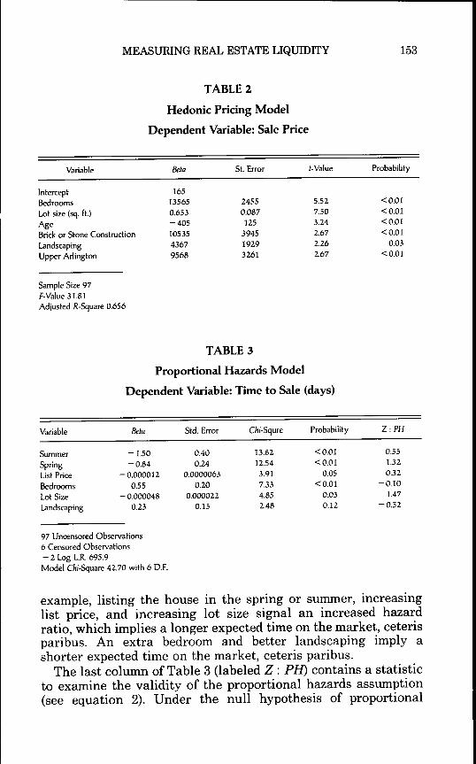
Using this data set, a hedonic pricing model was developedusing standard regression techniques, with sales price as thedependent variable.^ The beta coefficients for our hedonic pricingmodel are contained in Table 2. While models with greateroverall fit were possible, they included many insignificant vari-ables. The variables actually used were also selected to minimizemulticollinearity among the independent variables.
Table 3 contains the beta coefficients for the proportionalhazards model. These coefficients represent variables that affectthe time to sale: a negative beta means that increases in thevariable reduce the hazard rate: a positive beta signals thatincreases in the variable increase the hazard rate. In our
"OLS may not be appropriate for data sets with a considerable number ofcensored observations because there may be selectivity bias. In this case thehedonic estimates ought to be estimated using a correction procedure suggestedby Hekman. See Chapter 8 of Maddala [18] for a discussion of this procedure.
MEASURING REAL ESTATE LIQUTOITY 153
TABLE 2
Hedonic Pricing Model
Dependent Variable: Sale Price
Variable
InterceptBedroomsLot size (sq. ft.)AgeBrick or Stone ConstructionLandscapingUpper Arlington
example, listing the house in the spring or summer, increasinglist price, and increasing lot size signal an increased hazardratio, which implies a longer expected time on the market, ceterisparibus. An extra bedroom and better landscaping imply ashorter expected time on the market, ceteris paribus.
The last column of Table 3 (labeled Z : PH) contains a statisticto examine the validity of the proportional hazards assumption(see equation 2). Under the null hypothesis of proportional
154 KLUGER AND MILLER
TABLE 4
Liquidity Measure: The Price-Adjusted Odds Ratio
Odds Ratio
House listed in the Spring* 0.43House listed in the Summer* 0.22House with an Additional Bedroom 1.47Excellent Landscaping** 1.19Lot with an Additional 5000 square feet 0.76
*Relative to a house listed in the fall or winter**Relative to a house with good landscaping
hazards, the statistic will he a standard normal deviate. There-fore a Z : PH with a magnitude of 1.91 indicates that we cannotreject the null hypothesis of proportionality at the 5% signi-ficance level.'"
Our liquidity measure is hased on the coefficients of hoth theproportional hazards model and the hedonic pricing model.Recall that the PH model odds ratio is defined as exp()3(Zi - X^),where P represents the PH coefficients, and X., and Xj are thecharacteristics of the two houses to he compared. Using theestimated coefficients from the PH model, the relative odds ratiofor any house relative to any other house is:
ROR = exp[ - l.m*ASUMMER - 0.84* ASPRING
- 0.000012* ALIST PRICE+ 0.55* ABEDROOMS
+ 0.23*ALANDSCAPING-0.000048*zlLOT SIZE], (5)
where the A signifies the difference hetween the values of eachvariahle for the houses to he compared.
To calculate our relative liquidity measure, we compute theprice-adjusted odds ratio, or the relative odds ratio for eachhouse at market value." The price-adjusted odds ratios in Tahle4 were calculated using the preceding equation. For example,consider the relative odds ratio for two houses identical except
'"See Harrell and Lee [9] for a detailed discussion of this test."Note that the liquidity measure can be constructed using an estimate ofmarket value plus an estimate of the odds ratio. The estimate of market valuecould, for example, be obtained by appraisal. The estimate of the odds ratiocould be obtained from an alternative failure time model such as the Weibullmodel.
MEASURING REAL ESTATE LIQUIDITY 155
that one has an extra hedroom and is listed at a price of $13,565more (to refiect the market value of the extra hedroom asestimated hy the hedonic model in Tahle 2). The equation for theROR reduces to:
Therefore, we estimate that an additional hedroom will increasethe sale prohahility on any given day to 1.47 times what the saleprohahility would have heen without the extra hedroom. Thisnumher can he thought of as a measure of the "liquidity" addedhy an extra hedroom.'^
Tahle 4 contains the estimates of our liquidity measure foreach explanatory variahle in our illustrative PH model. For thedata set considered here, additional hedrooms and improvedlandscaping add to residential liquidity. Homes with larger lotswere found to he less liquid. We also report a strong seasonaleffect, with houses that are listed in spring or summer heing lessliquid.
THE LIQUIDITY MEASURE AND TIME ON THE MARKET
The measure of relative liquidity proposed here, the price-adjusted relative odds ratio, is clearly related to the expectedtime on the market. In the previous example, a house with anextra hedroom had a likelihood of sale on any given day that was1.47 times what the sale prohahility would have heen without theextra hedroom. Hence, the expected time on the market is lowerfor the house with an extra hedroom. Nevertheless, the odds ratioalone does not provide enough information to compute theexpected time on the market. An estimate of either the survivalfunction or the hazard function is required to calculate theexpected sale time.
Tahle 5 contains estimates of hoth the hazard function and thesurvival function for a house with median values for thevariahles in our sample. The "median" house (a house withmedian values for all the independent variahles in our data set) is
bedrooms were entered as a single variable taking values from two to sixbedrooms. The estimates from the PH model therefore represent the averageeffect of adding an additional bedroom. Alternatively, one could have coded thedata using separate dummy variables for a two-bedroom house, a three-bedroomhouse, and so on. In this case the model would give separate estimates for theliquidity of adding any number of bedrooms within the sample range.
156 KLUGER AND MILLER
TABLES
Estimated Survival and Hazard for the Median House*
*The median house is listed in the fall or winter with: three bedrooms, good landscaping, a 9490 square
foot lot and a list price of $54,540.
arbitrarily chosen to display the shape of the baseline hazardfunction. The hazard function represents the conditional prob-ability of sale for the "median home" at any point in time, andthe survival function represents the probability that a house willhave not yet sold at any point in time. These estimates plus thePH beta coefficients allow us to calculate the survival functionand the hazard function for any house of interest. Each hazardfunction will, by assumption, be proportional to the hazardfunction shown in Table 5. Equation (4') therefore simimarizesthe relationship between the hazard for the "median house" andthe hazard function for any other house. This relationshipimplies that the survival functions are not proportional, butrather related according toi ^
S(<,Z,) = S«,Z2)-p!« '- ^>' (6)
The survival function for each house can be used to roughlyestimate the expected sale time. Ths calculation can be carriedout using simple nimierical differentiation and integration pro-cedures on a personal computer. The expected time to sale for the
Miller [21, pp. 2-3] for the derivation of equation 6.
MEASURING REAL ESTATE LIQUIDITY 157
TABLE 6
Expected Sale Times (at the Listing Date)
Median House*
Median House except:Listed in SpringListed in SummerExtra Bedroom and List Price of $68,105Improved Landscaping and List Price of $58,907Extra 5000 Sq. Ft. of Lot and List Price of $57,805
Days39
6370303446
*The median house is listed in the fall or winter with: three bedrooms, good landscaping, a 9490 squarefoot lot and a list price of $54,540.
median home and for the median home with ceteris parihuschanges to the variahles in our data set are shown in Table 6."
For example, adding an extra hedroom to the median home(and increasing the cost of the home hy $13,565 to refiect theincrease in market value) reduces the expected sale time hy ninedays. Note that these calculations do not imply that adding anextra hedroom to a house other than the median will reduceexpected sale time hy a week. From the relative odds ratio, it isclear that expected sale time will he lower, hut it may he loweredhy more or less than a week depending on the other attrihutes ofthe houses.
CONCLUSION
The liquidity measure proposed in this paper is easy tocalculate and interpret. It is potentially useful to study themagnitudes of factors that affect liquidity. It is also tempting touse the proportional hazard estimates to examine the effects ofalternative pricing strategies on the time on the market. How-ever, one must he careful when evaluating pricing effects. It doesnot make sense to apply the proportional hazards estimates to ahouse with an asking price far away from its market value as thiswould he applying estimates from the model heyond the samplerange. For example, using our sample data set, a house priced
'•'These numbers are only ballpark estimates. Errors from estimating both thebeta coefficients and the baseline survival function are compounded with errorsfrom the numerical procedures due to the relatively small size of our data set.
158 KLUGER AND MILLER
$1000 less than its market price has an odds ratio of 0.98, aplausible estimate. A house priced $50,000 below market value,however, has an odds ratio of 0.55. This ratio is clearly too high,considering that the houses in this sample sell, on average, for$60,000.
Future research to determine the liquidity of various tj^jes ofreal estate in both active and thin markets will help expand ourunderstanding of the liquidity premium in real estate markets.
We would like to thank Don Haurin, Pat Hendershott and twoanonymous referees for helpful suggestions and comments.
REFERENCES
[1] American Institute of Real Estate Appraisers. The Appraisal ofReal Estate. AIREA, ninth edition 1987.
[2] J. H. Aldrich and F. D. Nelson. Linear Probability, Logit, andProbit Models. Sage, 1984.
[3] A. B. Atkinson and John Micklewright. Unemployment Benefitsand Unemployment Duration: A Study of Men in the UnitedKingdom in the 1970s. Suntory-Toyota International Centre forEconomics and Related Disciplines, 1985.
[4] J. Belkin, D. J. Hempel and D. W. McLeavey. An Empirical Studyof Time on the Market Using Multidimensional Segmentation ofHousing Markets. AREUEA Journal 4(3): 57-75. Fall 1976.
[5] J. Q. Butler and K. L. Guntermann. Housing Unit CharacteristicsSubdivision Sales Rates. Presented at the 1988 AREUEA meetings.
[6] D. R. Cox. Regression Models and Life-Tables. Journal ofthe RoyalStatistical Society 34(2): 187-220, May/August 1972.
[7] and D. Oakes. Analysis of Survival Data. Chapman &Hall, 1985.
[8] J. Green and J. B. Shoven. The Effects of Interest Rates onMortgage Prepayments. Journal of Money, Credit, and Banking18(1): 41—59, February 1986.
[9] F. E. Harrell, Jr. and K. L. Lee. Verifying the Assumptions of theCox Proportional Hazards Model. In Proceedings of the EleventhAnnual SAS Users Group International Conference. SAS Institute,Inc., 1986.
[10] D. R. Haurin. The Duration of Marketing Time of ResidentialHousing. AREUEA Journal 16(4): 396-410, Winter 1988.
[11] J. D. Kalbfleisch and R. L. Prentice. The Statistical Analysis ofFailure Time Data. Wiley, 1980.
[12] H. B. Kang and M. J. Gardner. Selling Price, Listing Price,Housing Features and Marketing Time in the Residential RealEstate Market. Presented at the 1988 AREUEA meetings.
MEASURING REAL ESTATE LIQUIDITY 159
[13] J. Kennan. The Duration of Contract Strikes in U.S. Manu-facturing. Journal of Econometrics 28(1): 5-28, April 1985.
[14] N. M. Kiefer. Economic Duration Data and Hazard Functions.Journal of Economic Literature 26(2): 646-79, June 1988.
[15] T. Lancaster. A Stochastic Model for the Duration of a Strike.Journal of the Royal Statistical Society 135(2): 257-71, April/June1972.
[16] E. T. Lee. Statistical Methods for Survival Data Analysis. LifetimeLearning Publications, 1980.
[17] S. A. Lippman and J. J. McCall. On Operational Measures ofLiquidity. American Economic Review 68(2): 43-55, March 1978.
[18] G. S. Maddala. Limited Dependent and Qualitative Variables inEconometrics. Cambridge University Press, 1983.
[19] N. G. Miller. Time on the Market and Selling Price. AREUEAJournal 6(2): 164-74, Summer 1978.
[20] and M. A. Sklarz. Pricing Strategies and ResidentialSelling Prices. The Journal of Real Estate Research 2(1): 31, 40, Fall1987.
[21] R. G. Miller, Jr. Survival Analysis. Wiley, 1981.[22] J. H. Wood and N. L. Wood. Financial Markets. Harcourt, Brace,