1

Measuring root system traits of wheat in 2D images to 1

parameterize 3D root architecture models 2

Magdalena Landl (1)*, Andrea Schnepf (1), Jan Vanderborght (1), A. Glyn Bengough (2, 3), Sara L. Bauke (4), 3

Guillaume Lobet (1), Roland Bol (1) and Harry Vereecken (1) 4

5

Affiliation 6

(1) Forschungszentrum Juelich GmbH, Agrosphere (IBG-3), D- 52428 Juelich, Germany 7

(2) The James Hutton Institute, Invergowrie, Dundee, DD2 5DA, UK 8

(3) School of Science and Engineering, University of Dundee, Dundee DD1 4HN, UK 9

(4) Institute of Crop Science and Resource Conservation (INRES) – Soil Science and Soil Ecology, University of 10

Bonn, Nussallee 13, 53115 Bonn, Germany 11

*Corresponding author: Email: m.landl@fz-juelich.de 12

13

*Corresponding author: 14

Magdalena Landl 15

Forschungszentrum Juelich GmbH, Agrosphere (IBG-3) 16

D- 52428 Juelich, Germany 17

Tel.: +49 2461 61 8835 18

Fax: +49 2461 61 2518 19

m.landl@fz-juelich.de 20

21

Number of text pages: 32 22

Number of tables: 6 23

Number of figures: 16 24

25

2

Keywords 26

axial root trajectories, branching angle, foraging performance, inter-branch distance, model parameterization, root 27

system architecture 28

Abstract 29

Background and aims The main difficulty in the use of 3D root architecture models is correct parameterization. We 30

evaluated distributions of the root traits inter-branch distance, branching angle and axial root trajectories from 31

contrasting experimental systems to improve model parameterization. 32

Methods We analyzed 2D root images of different wheat varieties (Triticum Aestivum) from three different sources 33

using automatic root tracking. Model input parameters and common parameter patterns were identified from 34

extracted root system coordinates. Simulation studies were used to (1) link observed axial root trajectories with 35

model input parameters (2) evaluate errors due to the 2D (versus 3D) nature of image sources and (3) investigate the 36

effect of model parameter distributions on root foraging performance. 37

Results Distributions of inter-branch distances were approximated with lognormal functions. Branching angles 38

showed mean values <90°. Gravitropism and tortuosity parameters were quantified in relation to downwards 39

reorientation and segment angles of root axes. Root system projection in 2D increased the variance of branching 40

angles. Root foraging performance was very sensitive to parameter distribution and variance. 41

Conclusions 2D image analysis can systematically and efficiently analyze root system architectures and parameterize 42

3D root architecture models. Effects of root system projection (2D from 3D) and deflection (at rhizotron face) on 43

size and distribution of particular parameters are potentially significant. 44

Abbreviations 45

β, root segment angle to the horizontal 46

∆β, reorientation angle of an individual root segment 47

De, diffusion coefficient of a solute in soil 48

ibd, inter-branch distance 49

3

IRC, inter-root competition 50

μ, mean value 51

σ, standard deviation of the random deflection angle (tortuosity) 52

sg, sensitivity to gravitropism 53

std, standard deviation 54

θ, branching angle in the vertical plane 55

Introduction 56

The efficiency of a plant root system to acquire below-ground resources predominantly depends on its root system 57

architecture (Lynch 2007; Rich and Watt 2013; Smith and De Smet 2012). The complex process of root system 58

development and its interaction with the soil matrix is, however, hard to study due to the opaque nature of the soil 59

which makes direct measurements difficult. The use of three - dimensional root architecture models can thereby 60

provide an opportunity to systematically investigate the influence of different environmental conditions and a wide 61

range of crop management regimes on the formation and functionality of root systems, to interpret experimental data 62

and to test hypotheses on root – soil interaction processes at different scales (Dunbabin et al. 2013; Roose and 63

Schnepf 2008). In experimental field studies, such large scale testing approaches are impossible to realize. An 64

important prerequisite for this simulation based investigation is that properties and behavior of the root system that 65

define its functioning in soils under different conditions can be inferred from experimental data. 66

Over the years, several three-dimensional root architectural models have been developed: RootMap (Diggle 1988), 67

R-SWMS (Javaux et al. 2008), RootBox (Leitner et al. 2010), SimRoot (Lynch et al. 1997), RootTyp (Pagès et al. 68

2004), SPACSYS (Wu et al. 2007). This diversity can be explained by the wide range of specific model objectives 69

such as representation of architectural characteristics of different species (Diggle 1988; Pagès et al. 2004), analysis 70

of interactions between root development and water and nutrient uptake (Dunbabin et al. 2002) or investigation of 71

root growth in structured soil (Landl et al. 2017). The gross representation of root systems, however, is comparable 72

in all these models and they use similar root architectural parameter sets: While the total size of a root system is 73

mainly determined by root traits regulating the branching density such as inter-branch distance, the shape or 74

4

distribution of a root system depends essentially on branching angle and root growth trajectories of the main axes 75

(Bingham and Wu 2011). Root growth trajectories of the main axes are determined by the directional orientation of 76

newly developed root segments. Due to the ability to use both space and time dimensions as well as various model 77

concepts, parameters that are used in models that generate root architectures can be defined in several ways. Table 1 78

gives an overview of the parameterization of the root traits inter-branch distance, branching angle and root growth 79

trajectories of the main axes for several individual root architecture models. 80

Differences in the parameterization of root traits leads to changes in root system architecture, which significantly 81

affects the ability of roots to forage the soil and thus the root nutrient uptake capacity (Fitter et al 1991; Pagès 2011). 82

Correct parameterization of 3D root architecture models is thus crucial when evaluating root-soil interaction 83

processes. 84

Root architecture parameterization techniques always represent a compromise between throughputs, precision, 85

realistic representation of field root architectures and ease of data processing (Kuijken et al. 2015). While 3D 86

imaging techniques such as x-ray computed tomography (Mooney et al. 2012; Tracy et al. 2012; Tracy et al. 2010) 87

and magnetic resonance imaging (Pohlmeier et al. 2013; Rascher et al. 2011) allow non – invasive studying of the 88

spatio – temporal dynamics of root growth, they still require elaborate data processing and are only suitable for 89

relatively small and young root systems scanned at low throughput rate (Mairhofer et al. 2012; Nagel et al. 2012). 90

Destructive sampling allows measurement of the whole root system, however, it is a time consuming and tedious 91

work, natural root positions can hardly be kept and a large loss of fine roots must be accepted (Judd et al. 2015; 92

Pagès and Pellerin 1994; Pellerin and Pagès 1994). In that sense, root parameterization via 2D image analysis 93

represents a good alternative by allowing for various methods of image acquisition, high throughput and – due to 94

recent developments of automated root tracking software – relatively simple processing (Delory et al. 2016; Leitner 95

et al. 2014). 96

Various methods for the acquisition of 2D root images have been developed over the years: The first 2D 97

representations of root system architecture were hand drawings (Kutschera 1960; Weaver et al. 1922; Weaver et al. 98

1924). The field grown root systems were thereby gradually excavated and simultaneously traced on sketching paper 99

(Kutschera 1960). A recently-revived method to non-invasively image the development of root system architecture in 100

2D is that of imaging roots grown in rhizotrons, and specifically rhizotron boxes (Kuchenbuch and Ingram 2002; 101

Nagel et al. 2012). Rhizotron boxes are soil filled containers with a transparent front plate that allows observing 102

5

dynamic changes in root system architecture. While rhizotrons enable better control of environmental influences on 103

root architecture development, they spatially constrict the root system and allow only partial visibility of roots at the 104

transparent front plate (Nagel et al. 2012; Nagel et al. 2015; Wenzel et al. 2001). A simple method that produces a 105

large number of images with perfect visibility of the root system is represented by roots grown on germination paper 106

(Atkinson et al. 2017; Atkinson et al. 2015). The absence of soil structure and soil mechanical impedance as well the 107

limited root age, however, cast doubt if the observed root architecture is a valid representation of root systems of 108

field grown plants (Clark et al. 2011; Hargreaves et al. 2009; Nagel et al. 2012). 109

In this study, we want to recover the root traits inter-branch distance, branching angle and root growth trajectories of 110

the main axes from various 2D root images of different wheat varieties (Triticum Aestivum). Model input parameters 111

and common parameter patterns are identified. In a series of simulation studies possible parameterization errors due 112

to the two-dimensionality of image sources as well as the influence of different parameterizations on root foraging 113

performance are evaluated. 114

Methods 115

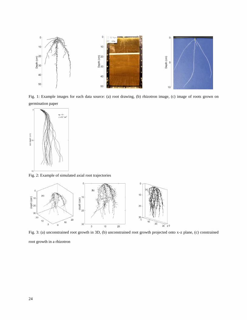
Image Sources 116

We used root images from three different sources: hand drawings from literature, images from a rhizotron 117

experiment and images from roots grown on germination paper (Fig.1). The 11 hand drawings with image 118

resolutions between 85 and 270 ppi were selected from three different literature sources and represent root systems 119

of variable age and wheat varieties growing at diverse locations (Table 2). The rhizotron images with a resolution of 120

300 ppi were obtained from an experimental study, in which spring wheat was grown under controlled laboratory 121

conditions in rhizotrons with inner dimensions of 50x30x3.5 cm. The lower part of the rhizotrons was filled with 122

compacted subsoil, the upper part with lose topsoil (bulk density 1.4 g cm-3

and 1 g cm-3

respectively). While the 123

experimental setup included different topsoil treatments with regard to phosphorus and water supply, we only used 124

the images of the six control replicates where both phosphorus and water supply was sufficient. The rhizotron images 125

were taken on day 41 after sowing, just before harvest. A detailed description of the experimental setup is given in 126

(Bauke et al. 2017). The images of roots grown on germination paper (24x30 cm) with a resolution of 442 ppi were 127

obtained from an experimental study, where two different winter wheat cultivars (‘Rialto’ and ‘Savannah’) were 128

6

grown in 41 respectively 39 replicates over a time period of 8 days under controlled lab conditions. A detailed 129

description of the experimental setup is given in Atkinson et al. (2015). 130

Image Analysis 131

Root system images were processed using the fully automatic root tracking software Root System Analyzer which is 132

based on MATLAB (R2014b) (RSA; Leitner et al. 2014). The RSA saves detailed information on the coordinates of 133

a root system in MATLAB mat-files. Analysis with the RSA requires images with continuous and clearly visible root 134

systems. The rhizotron images, where only part of the total root system is visible at the transparent front plate of the 135

rhizotron, thus had to be pre-processed prior to analysis. We used the open source tool GIMP 2.8 to segment the root 136

systems manually. To keep error propagation from image segmentation to parameter determination at a minimum, 137

we first only segmented those roots, which were clearly visible on the rhizotron image. These root systems were later 138

used for recovering the parameters branching angle and axial trajectories. We then additionally inserted laterals, for 139

which we had to estimate the location of the connection to their parent root. These extended root systems were later 140

used for recovering the parameter inter-branch distance, which depends on the visibility of all lateral roots. 141

Root Parameter Analysis 142

We parameterized the root traits inter-branch distance, branching angle and root growth trajectories of the main axes 143

from the extracted root system coordinates. The inter-branch distance was measured as the distance between two 144

successive branches in centimeters. The branching angle was determined as the angle in the vertical plane between a 145

branch and its parent root in degrees, which is measured at a certain distance from the point where the branch 146

emerges. In one respect, this distance should be minimized to measure the initial branching angle; however, it also 147

needs to be large enough to avoid inaccuracies in the computation process. We performed a small analysis based on 148

artificial root systems with known ground truth and similar root radii, which suggested that a search radius of 0.5 cm 149

distance from the branch point is suitable for correctly computing branching angles. Root growth trajectories of axial 150

roots are determined by their initial growth angle from the horizontal and its dynamic changes from the root base to 151

the root apex which is affected by numerous factors such as soil compaction (Popova et al. 2016), soil temperature 152

(Tardieu and Pellerin 1990) or soil water status (Nakamoto 1994). In a simplified way, the shape of a root trajectory 153

can be described by two features: its overall curvature and its small-scale waviness which is known as tortuosity 154

7

(Popova et al. 2016). To characterize the axial root trajectories from our data sources, we divided each root into 155

segments of 1 cm length and determined for each segment its angle to the horizontal as well as its reorientation angle 156

with respect to the previous root segment in degrees. We then calculated the relationship between growth angle and 157

reorientation angle of individual root segments, which gives information on the curvature of a trajectory in relation to 158

its inclination as well as on tortuosity. 159

Root parameters were quantified separately for each of the 11 root drawings. Root parameters derived from the six 160

rhizotron images obtained from replicate experiments were pooled together to one group. Root parameters derived 161

from images of roots grown on germination paper were classified into two groups according to cultivar (‘Rialto’: 39 162

images, ‘Savannah’: 41 images). Altogether, we analyzed root parameters from 14 different data sources. None of 163

the used image sources allowed differentiating between seminal and shoot-born roots and only one order of lateral 164

roots was identified. We therefore only distinguish between axial roots and first order laterals. 165

Simulation Studies 166

Among the different traits describing root architecture, root growth trajectories of axial roots are of particular 167

importance for the shape of a root system. Their correct representation in 3D root architecture models is thus 168

important to obtain plausible simulation results. In a first simulation study, we therefore tested the ability of different 169

model approaches to reproduce our experimental findings on axial root trajectories and quantified model parameters 170

for our analyzed root systems. 171

The recovery of 3D root architecture parameters from 2D images has the obvious drawback of losing the third 172

dimension. Images respectively drawings of root architectures are created by projecting the 3D root systems onto 2D 173

space. Root system architectures of plants grown in rhizotrons or on germination paper are affected by root 174

deflection due to spatial growth constraints. While this has no influence on the parameter inter-branch distance, both 175

branching angle and axial root growth trajectories are affected. In a second simulation study, we therefore analyzed 176

the effects of projection and deflection, respectively, on the parameters branching angle and axial root growth 177

trajectories. 178

Root architecture significantly influences root foraging performance by determining the volume of soil that can be 179

explored by roots (Fitter et al. 1991; Pagès 2011). In a third simulation study, we evaluated the effect of different 180

8

parameterizations of our focus root architecture parameters inter-branch distance, branching angle and axial root 181

growth trajectories on the foraging performance of root systems. 182

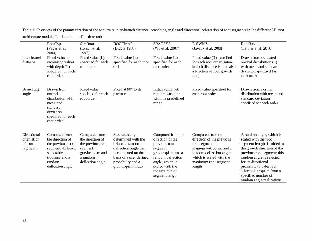
Simulation study 1: Ability of 3D root architecture models to reproduce experimental observations on axial root 183

trajectories 184

In 3D root architecture models, root growth trajectories are composed of individual root segments. At each root 185

growth time step, a new segment emerges whose directional orientation must be determined with regard to overall 186

curvature and tortuosity. Most root architecture models (SimRoot, RootTyp, SPACSYS, R-SWMS) use a vector-187

based approach, where the directional orientation of an individual root segment is calculated from a vector 188

expressing tortuosity and a vector expressing gravitropism. 2D root images represent root systems in the xz- plane 189

and thus provide information on root curvature and root tortuosity in vertical, but not in horizontal direction. To test 190

the ability of the vector-based approach to reproduce observations of axial root trajectories on 2D root images, we 191

thus converted the 3D equation to 2D space: 192

𝑑 = (𝑑𝑥𝛽,𝛿

𝑑𝑧𝛽,𝛿) + 𝑠𝑔 ∗ (

0−1

). (1) 193

The first term on the right hand side represents the growth direction vector of the preceding root segment dxβ with 194

unit length 1 which is deflected by the random angle δ; the second term expresses the gravitropism component with 195

sg as gravitropism sensitivity factor. The random deflection angle δ is a normally distributed random angle with 196

mean zero and unit standard deviation σ. The unknown parameters are thus the sensitivity to gravitropism sg and the 197

standard deviation of the random deflection angle σ (cf. Clausnitzer and Hopmans (1994)). We implemented this 198

formula in MATLAB and computed root trajectories using 7 different parameterizations of sg and 21 different 199

parameterizations of σ (147 parameter combinations altogether, values are given in Table 3). For each parameter 200

combination, we simulated 50 axial root trajectories with individual lengths of 50 cm (example in Fig.2). 201

Simulation study 2: Effects of projection and deflection on the parameters branching angle and axial root growth 202

trajectories. 203

The objective of this study was to analyze the effects of projection and deflection, respectively, on the parameters 204

branching angle and axial root growth trajectories. 205

9

Root system development was simulated using the MATLAB version of the 3D root architecture model RootBox, 206

which is fully described in Leitner et al. (2010) and shall here only be addressed briefly. RootBox defines each root 207

order by a set of different model parameters. Basal and apical root zone determine the length of the unbranched zone 208

before the first and after the last branch, respectively. Inter-branch distance defines the distance between two 209

successive branches and thereby also affects the maximum root length for a given number of branches. Root growth 210

speed is described by a negative exponential function whose initial slope is determined by the initial elongation rate 211

and whose asymptote depends on the maximum root length. The emergence angle of axial roots respectively the 212

initial angle between a branch and its parent root is defined by a radial angle in the horizontal plane, and an insertion 213

respectively branching angle in the vertical plane. The radial angle is generally drawn at random between 0 and 2π, 214

but can also be set to a specific angle to consider non-independence of branching files. To describe axial root growth 215

trajectories, we implemented the vector-based approach used in most root architecture models (SimRoot, RootTyp, 216

SPACSYS, R-SWMS) into RootBox: In this approach, newly emerged root segments are oriented according to the 217

direction of the previous root segment, sensitivity to gravitropism and random angle deflection. 218

To evaluate the effect of projection, we mapped the unconstrained 3D root system onto the x-z plane. To evaluate the 219

effect of deflection, we simulated a root system, which was spatially constrained by a rhizotron with dimensions of 220

20x2x30 cm (Fig.3). This geometry is implemented based on signed distance functions in which the distance of a 221

given point to the closest boundary is evaluated and given a positive sign if located inside the geometry and a 222

negative sign if located outside. Random optimization ensures that the new position of a growing root tip is always 223

inside the rhizotron domain (Leitner et al. 2010). Using the coordinates of these root systems, we then computed (1) 224

branching angles between laterals and their parent roots and (2) relationships between angle to the horizontal and 225

reorientation angle of individual root segments. 226

Simulation study 3: Influence of different parameterizations of inter-branch distance, branching angle and axial root 227

trajectories on foraging performance of a root system 228

Root system development was simulated using the MATLAB version of the 3D root architecture model RootBox 229

with an alternative approach for the simulation of axial root growth trajectories as described in simulation study 2. 230

The soil volume around a root system available for nutrient uptake, i.e. the rhizosphere, was computed using the 231

approach by Fitter et al. (1991). For this procedure, a very fine 3D grid is overlaid on the root system. The center of 232

10

every grid cell is then scanned for its distance to the nearest root segment. If the distance is smaller than a specified 233

rhizosphere radius Rrhiz, the grid cell volume is counted as rhizosphere volume. The rhizosphere radius Rrhiz is 234

determined by the effective diffusion coefficient of a solute in soil and the age of the respective root segment and 235

calculated according to Nye and Tinker (1977) as 236

𝑅𝑟ℎ𝑖𝑧 = 𝑟 + 2√𝐷𝑒 𝑡, (2) 237

where r is the radius of the root segment (cm), De is the effective diffusion coefficient in soil (cm2s

-1) and t is the root 238

segment age (s). To evaluate the influence of different soil diffusion coefficients (De) on the rhizosphere volume, we 239

performed simulations with three different De values: 10-8

, 10-7

and 2x10-6

cm² s-1

. The first two values are typical 240

effective phosphorus diffusion coefficients in soil, which account for the effect of sorption of phosphorus to soil 241

particles (Schenk and Barber 1979); the latter one is a characteristic nitrate diffusion coefficient of the soil (Volder et 242

al. 2005). While the net rhizosphere volume was defined as the volumetric sum of all unique grid cells, the 243

rhizosphere volume with overlap was specified as the volumetric sum of all - partially multiply assigned - grid cells. 244

The overlap volume is then the difference between rhizosphere volume with overlap and net rhizosphere volume 245

(Fig.4). Considering that both rhizosphere and overlap volume are absolute values and depend on the total size of a 246

root system, we introduced the parameter inter-root competition (IRC) as a size-independent measure of comparison 247

following the approach by Ge et al. (2000). IRC is calculated as 248

𝐼𝑅𝐶 =𝑉𝑜𝑣𝑒𝑟𝑙𝑎𝑝

𝑉𝑟ℎ𝑖𝑧𝑜∗ 100%, (3) 249

where Voverlap is the overlap volume and Vrhizo is the net rhizosphere volume. Fig.5 shows an example of a simulated 250

root system and its surrounding rhizosphere volume for different values of De. 251

Using observations from root image analysis, we identified factors that can be used to differently parameterize our 252

three focus parameters. These factors were mean and standard deviation for both inter-branch distance and branching 253

angle and standard deviation of the random angle deflection respectively sensitivity to gravitropism for the parameter 254

axial root growth trajectories. For each of these factors, we defined variation intervals with lower and upper bounds. 255

For the parameter inter-branch distance, we used probability distribution as an additional categorical factor of 256

variation, which was set to either normal or lognormal distribution. Descriptive statistics of the lognormal 257

distribution were calculated by transformation from the parameters of the normal distribution. The domain of the 258

11

normal distribution was restricted to the positive number range; negative values were set to 10-6

cm. We also 259

included a categorical factor of variation for the radial alignment of 1st order laterals around the main axis. In 260

literature, the alignment of lateral roots around the root axis is still unclear. While Abadia-Fenoll et al. (1986) and 261

Barlow and Adam (1988) found lateral roots of onion and tomato to form in acropetal sequence around their parent 262

axis, Pellerin and Tabourel (1995) and Yu et al. (2016) observed an unpredictable radial emergence pattern for lateral 263

roots of maize and wheat. Due to these inconsistencies, we specified the radial angle either as random in the interval 264

[0 2π] or set it to a value of 45 ° (sequential acropetal branching from 8 phloem poles around the axis). Variation 265

intervals for parameterization factors as well as descriptions of the additional factors are given in Table 4. The 266

remaining root growth parameters were set to fixed values, which were either derived from literature or directly from 267

our analyzed root images (Table 5). We considered two orders of lateral roots. The simulation time was set to 30 268

days and each root system consisted of 7 axial roots. 269

For all possible combinations of categorical factors, we then performed 1000 root system realizations that 270

corresponded with 1000 parameter sets that were randomly drawn from the intervals specified in Table 4. This gave 271

a total of 4000 root system realizations (i.e.22x1000). For each root system, we then computed inter-root competition 272

as a measure of foraging performance for all three soil diffusion coefficients (De) defined above. Relationships 273

between inter-root competition and our focus parameters were explored by means of scatterplots. To visualize the 274

main trends, we fitted linear regression lines. Correlation analyses were then used to quantitatively evaluate the 275

linear relationship between inter-root competition and our focus parameters. 276

Statistics 277

Statistical analyses were performed with MATLAB (R2014b). To evaluate differences in means with unequal 278

variance, a Welch’s t-test was used. To analyze differences in variances, we performed a two-sample F-test. Linear 279

regression relationships were evaluated by means of an F-test. In the following, significant results correspond to 280

p<0.05, while highly significant results represent p<0.01. 281

12

Results 282

Inter-branch distance 283

The relationships between inter-branch distance and distance along the root axis are very scattered for all data 284

sources with values ranging from close to 0 cm to up to 3 cm. An F-test showed a significant increase in inter-branch 285

distance from the base of the branched zone down to the root apex for 11 out of 14 data sets, no trend for two data 286

sets and a decrease for one data set (Fig.6). The large variability of inter-branch distances observed for the data 287

source from rhizotron images can be explained by the only partial visibility of the root system which has probably 288

obscured some lateral roots. The global distributions show for all data sources a highly asymmetrical shape which 289

can be well described with lognormal distributions (Fig.7). We observed a large percentage of short inter-branch 290

distances with medians ranging between 0.1 and 0.5 cm (Fig.8). No systematic pattern was apparent with regard to 291

the different data sources. 292

Branching angle 293

The global distribution of branching angles shows a bell shape for the roots grown on germination paper that can be 294

approximated with a normal distribution; for the remaining data sources, the distribution of branching angles is 295

spread more widely and shows positive skewness (Fig.9). Interestingly, branching angles from all data sources show 296

similar medians that range from 59.5° to 79.4° and are well below 90° (Fig.10). 297

Root growth trajectories 298

Root growth trajectories of axial roots were reconstructed for all root systems of each data source from the extracted 299

root coordinates prior to analysis (Fig.11). 300

There was a negative relationship between reorientation angle and angle of the previous 1 cm long root segment for 301

all but one data source meaning that more horizontally growing roots generally reoriented stronger towards the 302

vertical than more perpendicularly growing ones (Fig.12). An F-test showed that this correlation was highly 303

significant for 3, significant for 5 and not significant for 6 data sources. Not significant relationships can be an 304

indicator for abrupt changes in the growth path (e.g. the rightmost trajectory in Fig 11a), high root tortuosity or 305

liminal growth angles that deviate from the vertical (Nakamoto 1994). The reorientation angle ∆β at a segment angle 306

13

of β=-90° (vertical root growth) predicted by regression tended for all data sources towards zero suggesting that 307

gravitropism is the predominant influence factor in the formation of trajectory curvature. While the slope of the 308

regression line is a measure of gravitropism, the standard error of the estimate determines the degree of root 309

tortuosity. The slope of the regression lines ranged between 0 and -0.2; the standard error of the estimate between 310

7.7 ° and 21.8 °. With regard to different data sources, we did not find any systematic pattern of slope; standard 311

errors of the estimate, however, were highest for root drawings of large, mature root systems and lowest for roots 312

grown on germination paper. 313

Simulation studies 314

Simulation study 1: Ability of 3D root architecture models to reproduce experimental observations on axial root 315

trajectories 316

For each combination of parameters describing gravitropism and tortuosity, we calculated the relationship between 317

reorientation angle ∆β and angle of the previous 1 cm long root segment β and approximated it with a linear 318

regression line. The results are shown in Fig.13 for 20 selected parameter combinations. The standard deviation of 319

the random deflection angle σ can be seen as a direct measure of the standard error of the estimate and thus tortuosity 320

if the influence of gravitropism is not too strong. Large values of gravitropism force the root tip to grow towards the 321

vertical and result in standard errors of the estimate smaller than σ. The gravitropism parameter sg is inversely 322

proportional to the slope of the regression line. The prediction with the regression lines, which are close to 0° at β= -323

90°, reflect the minimum average reorientation of vertically oriented roots. An F-test showed that correlations 324

between reorientation angle and angle of the previous 1 cm long root segment were highly significant for all 325

combinations, except for the combination of the largest root tortuosity and smallest gravitropism value. The 326

relationships between root reorientation and root angle resemble those calculated for our image-derived axial root 327

trajectories (Fig.12). The approach is thus well suited to simulate curvature and tortuosity of wheat root trajectories. 328

To link the model parameters necessary for the simulation of root trajectories (sensitivity to gravitropism sg and root 329

tortuosity σ) to the relationship between root reorientation and root segment angle, we calculated characteristic 330

curves for the different parameter combinations (Fig.14). The characteristic curves are the smoothed connection lines 331

between the properties of the regression lines (standard error of the estimate and slope) that relate segment angles 332

and reorientation angles of axial root trajectories for each parameter combination. Figure 14 shows that slope and 333

14

standard error of the regression cannot be mapped linearly to the parameters σ and sg that describe gravitropism and 334

tortuosity. To quantify model parameters for our observed root trajectories, we inserted the regression line properties 335

deduced from Fig.12 into the graphs and located their positions. This gave us values between 0.01 and 0.3 for the 336

sensitivity to gravitropism sg and values between 9 and 20 °cm-1

for the unit standard deviation of the random angle 337

σ. 338

Simulation study 2: Effects of projection and deflection on the parameters branching angle and axial root growth 339

trajectories. 340

While mean branching angles of projected and deflected root systems did not differ significantly from branching 341

angles of the unconstrained 3D root system, their variance was significantly higher. This was especially true for the 342

projected root system (Fig.15-1). The similarity in mean branching angles can be explained by the symmetrical 343

alignment of lateral roots around the root axis, which leads to a compensation between positive and negative angle 344

deviations due to projection or deflection. Relationships between reorientation angle and angle of the previous 1 cm 345

long root segment differed significantly between projected and deflected root systems and the unconstrained 3D root 346

system with regard to slope and thus gravitropic root growth. With regard to standard deviation of the estimate and 347

thus tortuosity, only the projected, but not the deflected root system showed a significantly higher value than the 348

unconstrained 3D root system (Fig.15-2). Considering that absolute deviations are rather small, these discrepancies 349

in gravitropism and tortuosity are negligible in terms of model parameterization. 350

Simulation study 3: Influence of different parameterizations of inter-branch distance, branching angle and axial root 351

trajectories on foraging performance of a root system 352

We found clear relationships between inter-root competition and different parameterizations. These relationships are 353

illustrated for De = 10-8

cm²s-1

in Fig.16. In each plot, all simulation results were plotted against the specific 354

parameter. In Table 6, correlation coefficients show the significance of linear relationships between inter-root 355

competition and parameters. As expected, IRC decreased with increasing mean inter-branch distance. If mean inter-356

branch distance was low, IRC was significantly higher for lognormally than for normally distributed inter-branch 357

distances. Regular alignment of laterals around the main axis tended to less IRC than random alignment, however, 358

not significantly. The relationship between IRC and mean inter-branch distance was significantly weaker for the 359

largest soil diffusion coefficient. The effect of varying standard deviation of inter-branch distance on IRC was 360

15

surprising: For lognormally distributed inter-branch distances IRC increased with increasing standard deviation; for 361

normally distributed inter-branch distances, it decreased. These relationships remained nearly constant for all soil 362

diffusion coefficients. IRC decreased with increasing mean branching angle. This effect, however, was only 363

significant for the lowest soil diffusion coefficient. Larger standard deviations of the branching angle led to a 364

significant increase in IRC for the lower two soil diffusion coefficients. This effect was larger for regularly aligned 365

laterals than for randomly aligned ones. Greater values of standard deviation of the random angle deflection led to 366

lower IRC. This effect, however, was only significant for the largest soil diffusion coefficient. As expected, larger 367

values of sensitivity to gravitropism led to more IRC. This effect was stronger for larger soil diffusion coefficients 368

and also for root systems with normally distributed inter-branch distances as compared with lognormally distributed 369

ones. 370

Discussion 371

2D image analysis is a simple and fast way to retrieve information on root system architectures for the 372

parameterization of 3D root architecture models. The systematic analysis of root images from three different sources 373

(root drawings, rhizotron images, images of roots grown on germination paper) allowed us to identify universally 374

occurring parameter patterns of wheat roots. 375

Observed patterns of root architecture parameters contrast common model assumptions 376

Inter-branch distance along axial roots predominantly increased with increasing distance from the base of the 377

branched zone. But in some cases, it also remained constant or decreased. These results are in line with published 378

data: While inter-branch distance along the axial roots was frequently observed to increase with increasing distance 379

from the base of the branched zone (e.g. maize by Ito et al. (2006), Pagès and Pellerin (1994), Postma et al. (2014) 380

and pea by Tricot et al. (1997)), other studies found constant or no identifiable pattern of inter-branch distance along 381

axial roots (e.g. wheat by Ito et al. (2006) and banana by Draye (2002)). Studies have proposed that soil compaction 382

(Pagès and Pellerin 1994), oxygen gradients (Liang et al. 1996) or water availability in the vicinity of the root (Bao 383

et al. 2014) may alter branching density and thus inter-branch distances. In 3D root architecture models, the 384

phenomenon of varying inter-branch distances along axial roots could be considered by a coefficient that is linked to 385

these processes. Our findings suggest that the global distribution of inter-branch distances of wheat roots follows a 386

lognormal distribution, which is in line with observations by Pagès (2014) on roots of various species of the Poaceae 387

16

family and Le Bot et al. (2010) on the root system of a tomato plant. This contrasts common assumptions of 3D root 388

architecture models where inter-branch distances are either set to a fixed value or drawn from a normal distribution 389

(see Table 1). 390

The branching angle of lateral roots relative to their parent axis is a standard parameter that is included in all 3D root 391

architecture models (Table 1) and defines the initial direction of the first segment of a lateral root at the point of 392

emergence. Our findings suggest that branching angles of 1st order laterals of wheat root systems are significantly 393

smaller than 90° with a variance that depends on the growth medium. This contrasts common model assumptions 394

where branching angles are frequently set to a constant value of 90° relative to the parent root for reasons of 395

simplicity (Clausnitzer and Hopmans 1994; Pagès et al. 2004; Wu et al. 2005) or as a general model condition 396

(Diggle 1988). 397

More horizontally growing roots reoriented stronger towards the vertical than more vertically growing roots with 398

reorientation angles approaching 0 ° as the roots turn to the vertical. These findings are in line with observations by 399

Wu et al. (2015) on axial maize root trajectories. A number of axial root trajectories derived from root drawings did 400

not follow a continuous gravitropic growth path, but changed their slope abruptly to the vertical after growing in 401

relatively constant direction. Similar observations were reported by Tardieu and Pellerin (1990) who suggest that 402

earthworm channels that can be used by roots as preferential growth paths might be responsible for this effect. Levels 403

of root tortuosity showed a relatively clear ranking with tortuosity of root systems grown in structured soil > 404

tortuosity of roots grown in sieved soil > tortuosity of roots grown on filter paper. While root age seems to have an 405

influence, this effect is probably also caused by differences in the penetration resistance of the growth medium as 406

proposed by Popova et al. (2016). A simulation study showed good agreement between simulated and observed 407

curvature and tortuosity of axial wheat root trajectories. We developed characteristic curves that relate model input 408

parameters with downwards reorientation and segment angles of axial trajectories. These characteristic curves can be 409

used to calibrate the model parameters gravitropism and tortuosity from 2D root trajectories, which is a step forward 410

in the realistic parameterization of 3D root architecture models. 411

Root system projection leads to overestimation of the variance of branching angles 412

The use of two-dimensional root drawings or rhizotron images for the parameterization of 3D root architecture 413

models is common practice (Delory et al. 2016; Doussan et al. 2006; Leitner et al. 2014; Pagès et al. 2004). To our 414

17

knowledge, the effects of root system projection or deflection on size and distribution of 3D root architecture 415

parameters, however, has not yet been analyzed. We showed that projection greatly affects branching angles by 416

overestimating their variance. Effects of projection and deflection, respectively, on tortuosity and gravitropism 417

parameters were shown to be negligible. 418

Root foraging performance depends strongly on parameter distribution and parameter variance 419

The influence of the main determinants of root architecture (e.g. mean inter-branch distance, mean branching angle) 420

on root foraging performance is well documented in literature (Bingham and Wu 2011; Postma et al. 2014). The 421

influence of parameter variance and distribution, however, which describes the degree to which stochasticity affects 422

developmental processes, is much less explored (Forde 2009). In most 3D root architecture models, parameter 423

stochasticity is not used or only used to a limited extent (Table 1). We could demonstrate the significant impact of 424

variance in both inter-branch distance and branching angle on foraging performance of a root system. Also, the use 425

of different distributions of inter-branch distance (normal, lognormal) led to significant differences in effective 426

rhizosphere volume around a root system. Interestingly, differences in radial alignment of lateral roots around the 427

root axis, i.e. random or acropetal branching, only led to minor differences in root foraging performance. 428

We chose the model approach by Nye and Tinker (1977) to compute the rhizosphere volume around a root system. 429

This purely physical model assumes continuous nutrient uptake by individual root segments. Gao et al. (1998) and 430

Bouma et al. (2001), however, showed that root segment age is inversely related to nutrient uptake capacity and that 431

young roots therefore take up more nutrients than old roots. Inter-root competition is mainly caused by rhizosphere 432

zone overlap of neighboring laterals, which are usually of similar age. Taking into account root segment age-433

dependent nutrient uptake rates would therefore alter absolute values of root foraging performance, but not our 434

described qualitative relationships and trends. 435

This study improves the capacity of modelers to simulate realistic root systems, which can be used to investigate 436

root-soil interaction processes. Further investigations could include research on parameters that were not the focus of 437

this study, but also greatly influence root foraging performance such as number of axial roots, axial insertion angle 438

and length and distribution of lateral roots. More information on root architecture parameters for a range of plant 439

species would also be desirable. Increased knowledge on plastic root response to soil heterogeneity and 440

environmental changes would further improve 3D root architecture modeling. 441

18

Acknowledgements 442

Funding by German Research Foundation within the Research Unit DFG PAK 888 is gratefully acknowledged. The 443

James Hutton Institute receives funding from the Scottish Government. We also thank Klaas Metselaar from the 444

Department of Environmental Sciences at Wageningen University, Netherlands, for providing high-resolution scans 445

of wheat root images from the Root Atlas. 446

447

19

Abadia-Fenoll F, Casero P, Lloret P, Vidal M 1986 Development of lateral primordia in decapitated adventitious 448

roots of Allium cepa. Ann. Bot. 58, 103-107 449

Atkinson JA, Lobet G, Noll M, Meyer PE, Griffiths M, Wells DM 2017 Combining semi-automated image analysis 450

techniques with machine learning algorithms to accelerate large scale genetic studies. GigaScience 6, 1-7 451

Atkinson JA, Wingen LU, Griffiths M, Pound MP, Gaju O, Foulkes MJ, Le Gouis J, Griffiths S, Bennett MJ, King J 452

2015 Phenotyping pipeline reveals major seedling root growth QTL in hexaploid wheat. J. Exp. Bot. 66, 453

2283-2292 454

Bao Y, Aggarwal P, Robbins NE, Sturrock CJ, Thompson MC, Tan HQ, Tham C, Duan L, Rodriguez PL, Vernoux 455

T, Mooney SJ, Bennett MJ, Dinneny JR 2014 Plant roots use a patterning mechanism to position lateral root 456

branches toward available water. Proc. Natl. Acad. Sci. U. S. A.111, 9319-9324 457

Barlow P, Adam J 1988 The position and growth of lateral roots on cultured root axes of tomato,Lycopersicon 458

esculentum (Solanaceae). Plant Syst. Evol. 158, 141-154 459

Bauke SL, Landl M, Koch M, Hofmann D, Nagel KA, Siebers N, Schnepf A, Amelung W 2017 Macropore effects 460

on phosphorus acquisition by wheat roots – a rhizotron study. Plant Soil 416, 67-82 461

Bingham IJ, Wu L 2011 Simulation of wheat growth using the 3D root architecture model SPACSYS: validation and 462

sensitivity analysis. Eur. J. Agron.34, 181-189 463

Bouma TJ, Yanai RD, Elkin AD, Hartmond U, Flores‐Alva DE, Eissenstat DM 2001 Estimating age‐dependent costs 464

and benefits of roots with contrasting life span: comparing apples and oranges. New Phytol. 150, 685-695 465

Clark RT, MacCurdy RB, Jung JK, Shaff JE, McCouch SR, Aneshansley DJ, Kochian LV 2011 3-dimensional root 466

phenotyping with a novel imaging and software platform. Plant Physiol 156, 455-465 467

Clausnitzer V, Hopmans J 1994 Simultaneous modeling of transient three-dimensional root growth and soil water 468

flow. Plant Soil 164, 299-314 469

Delory BM, Baudson C, Brostaux Y, Lobet G, Du Jardin P, Pagès L, Delaplace P 2016 archiDART: an R package 470

for the automated computation of plant root architectural traits. Plant Soil 398, 351-365 471

Diggle AJ 1988 ROOTMAP - a model in three-dimensional coordinates of the growth and structure of fibrous root 472

systems. Plant Soil 105, 169-178 473

Doussan C, Pierret A, Garrigues E, Pagès L 2006 Water uptake by plant roots: II-Modelling of water transfer int he 474

soil root-system with explicit accoutn of flow within the root system - Comparison with experiments. Plant 475

Soil 283, 99-117 476

20

Draye X 2002 Consequences of root growth kinetics and vascular structure on the distribution of lateral roots. Plant, 477

Cell Environ. 25, 1463-1474 478

Dunbabin V, Diggle AJ, Rengel Z, van Hugten R 2002 Modelling the interactions between water and nutrient uptake 479

and root growth. Plant Soil 239, 19-38 480

Dunbabin VM, Postma JA, Schnepf A, Pagès L, Javaux M, Wu L, Leitner D, Chen YL, Rengel Z, Diggle AJ 2013 481

Modelling root–soil interactions using three–dimensional models of root growth, architecture and function. 482

Plant Soil 372, 93-124 483

Fitter A, Stickland T, Harvey M, Wilson G 1991 Architectural analysis of plant root systems 1. Architectural 484

correlates of exploitation efficiency. New Phytol.118, 375-382 485

Forde BG 2009 Is it good noise? The role of developmental instability in the shaping of a root system. J. Exp. Bot. 486

60, 3989-4002 487

Gao S, Pan WL, Koenig RT 1998 Integrated root system age in relation to plant nutrient uptake activity. Agron. J. 488

90, 505-510 489

Ge Z, Rubio G, Lynch JP 2000 The importance of root gravitropism for inter-root competition and phosphorus 490

acquisition efficiency: results from a geometric simulation model. Plant Soil 218, 159-171 491

Hargreaves CE, Gregory PJ, Bengough AG 2009 Measuring root traits in barley (Hordeum vulgare ssp. vulgare and 492

ssp. spontaneum) seedlings using gel chambers, soil sacs and X-ray microtomography. Plant Soil 316, 285-493

297 494

Ito K, Tanakamaru K, Morita S, Abe J, Inanaga S 2006 Lateral root development, including responses to soil drying, 495

of maize (Zea mays) and wheat (Triticum aestivum) seminal roots. Physiol. Plant. 127, 260-267 496

Javaux M, Schröder T, Vanderborght J, Vereecken H 2008 Use of a Three-Dimensional Detailed Modeling 497

Approach for Predicting Root Water Uptake. Vadose Zone J. 7, 1079-1079 498

Judd LA, Jackson BE, Fonteno WC 2015 Advancements in root growth measurement technologies and observation 499

capabilities for container-grown plants. Plants 4, 369-392 500

Kuchenbuch R, Ingram K 2002 Image analysis for non-destructive and non-invasive quantification of root growth 501

and soilw ater content in rhizotrons. J. Plant Nutr. Soil Sci. 165, 573-581 502

Kuijken RC, van Eeuwijk FA, Marcelis LF, Bouwmeester HJ 2015 Root phenotyping: from component trait in the 503

lab to breeding. J. Exp. Bot. 66, 5389-5401 504

21

Kutschera L 1960 Wurzelatlas mitteleuropäischer Ackerunkräuter und Kulturpflanzen. DLG-Verlag, Frankfurt/Main. 505

pp. 124, 574 506

Kutschera L, Lichtenegger E, Sobotik M 2009 Wurzelatlas der Kulturpflanzen gemäßigter Gebiete: mit Arten des 507

Feldgemüsebaues. DLG-Verlag Frankfurt/Main. pp. 222, 226-227 508

Landl M, Huber K, Schnepf A, Vanderborght J, Javaux M, Bengough AG, Vereecken H 2017 A new model for root 509

growth in soil with macropores. Plant Soil 415, 99-116 510

Le Bot J, Serra V, Fabre J, Draye X, Adamowicz S, Pagès L 2010 DART: a software to analyse root system 511

architecture and development from captured images. Plant Soil 326, 261-273 512

Leitner D, Felderer B, Vontobel P, Schnepf A 2014 Recovering root system traits using image analysis exemplified 513

by two-dimensional neutron radiography images of lupine. Plant Physiol 164, 24-35 514

Leitner D, Klepsch S, Bodner G, Schnepf A 2010 A dynamic root system growth model based on L-Systems. Plant 515

Soil 332, 177-192 516

Liang J, Zhang J, Wong M 1996 Effects of air-filled soil porosity and aeration on the initiation and growth of 517

secondary roots of maize (Zea mays). Plant Soil 186, 245-254 518

Lynch JP 2007 Roots of the second green revolution. Aust. J. Bot. 55, 493-512 519

Lynch JP, Nielsen KL, Davis RD, Jablokow AG 1997 SimRoot: modelling and visualization of root systems. Plant 520

Soil 188, 139-151 521

Mairhofer S, Zappala S, Tracy SR, Sturrock C, Bennett M, Mooney SJ, Pridmore T 2012 RooTrak: automated 522

recovery of three-dimensional plant root architecture in soil from X-ray microcomputed tomography images 523

using visual tracking. Plant Physiol 158, 561-569 524

Mooney SJ, Pridmore TP, Helliwell J, Bennett MJ 2012 Developing X-ray computed tomography to non-invasively 525

image 3-D root systems architecture in soil. Plant Soil 352, 1-22 526

Nagel K, Putz A, Gilmer F, Heinz K, Fischbach A, Pfeifer J, Faget M, Bloßfeld S, Ernst M, Dimaki C, Kastenholz B, 527

Kleinert A, Galinski A, Scharr H, Fiorani F, Schurr U 2012 GROWSCREEN-Rhizo is a novel phenotyping 528

robot enablign simultaneous measruements of root and shoot growth for pkants grown in soil-filled 529

rhizotrons. Funct. Plant Biol. 39, 891-904 530

Nagel KA, Bonnett D, Furbank R, Walter A, Schurr U, Watt M 2015 Simultaneous effects of leaf irradiance and soil 531

moisture on growth and root system architecture of novel wheat genotypes: implications for phenotyping. J. 532

Exp. Bot. 66, 5441-5452 533

22

Nakamoto T 1994 Plagiogravitropism of maize roots. Plant Soil 165: 327-332. 534

Nye PH, Tinker PB 1977 Solute movement in the soil-root system. Univ of California Press. pp. 342 535

Pagès L 2011 Links between root developmental traits and foraging performance. Plant, Cell Environ. 34, 1749-1760 536

Pagès L, Pellerin S 1994 Evaluation of parameters describing the root system architecture of field grown maize 537

plants (Zea mays L.),II. Plant Soil 164, 169-176 538

Pagès L, Picon‐Cochard, Catherine 2014 Modelling the root system architecture of Poaceae. Can we simulate 539

integrated traits from morphological parameters of growth and branching? New Phytol.204, 149-158 540

Pagès L, Vercambre G, Drouet J-L, Lecompte F, Collet C, Le Bot J 2004 Root Typ: a generic model to depict and 541

analyse the root system architecture. Plant Soil 258, 103-119 542

Pellerin S, Pagès L 1994 Evaluation of parameters describing the root system architecture of field grown maize 543

plants (Zea mays L.), I. Plant Soil 164, 155-167 544

Pellerin S, Tabourel F 1995 Length of the apical unbranched zone of maize axile roots: its relationship to root 545

elongation rate. Environ. Exp. Bot. 35, 193-200 546

Pohlmeier A, Javaux M, Vereecken H, Haber-Pohlmeier S 2013 Magnetic resonance imaging techniques for 547

visualization of root growth and root water uptake processes. In: S. H. Anderson, J. W. Hopmans, editors, 548

Soil–Water–Root Processes: Advances in Tomography and Imaging. pp. 137-156. SSSA Spec. Publ. 61 549

Popova L, van Dusschoten D, Nagel KA, Fiorani F, Mazzolai B 2016 Plant root tortuosity: an indicator of root path 550

formation in soil with different composition and density. Ann. Bot. 118, 685-698 551

Postma JA, Dathe A, Lynch JP 2014 The optimal lateral root branching density for maize depends on nitrogen and 552

phosphorus availability. Plant Physiol 166, 590-602 553

Rascher U, Blossfeld S, Fiorani F, Jahnke S, Jansen M, Kuhn AJ, Matsubara S, Märtin LL, Merchant A, Metzner R 554

2011 Non-invasive approaches for phenotyping of enhanced performance traits in bean. Funct. Plant Biol. 555

38, 968-983 556

Rich S, Watt M 2013 Soil conditions and cereal root system architecture: review and considerations for linking 557

Darwin and Weaver. J. Exp. Bot. 64, 1193-1208 558

Roose T, Schnepf A 2008 Mathematical models of plant–soil interaction. Philos. Trans. R. Soc., A 366, 4597-4611 559

Schenk M, Barber S 1979 Phosphate uptake by corn as affected by soil characteristics and root morphology. Soil Sci. 560

Soc. Am. J. 43, 880-883 561

23

Smith S, De Smet I 2012 Root system architecture: insights from Arabidopsis and cereal crops. Philos. Trans. R. 562

Soc., B 367, 1441-1452 563

Tardieu F, Pellerin S 1990 Trajectory of the nodal roots of maize in fields with low mechanical constraints. Plant 564

Soil 124, 39-45 565

Tracy SR, Black CR, Roberts JA, Sturrock C, Mairhofer S, Craigon J, Mooney SJ 2012 Quantifying the impact of 566

soil compaction on root system architecture in tomato (Solanum lycopersicum) by X-ray micro-computed 567

tomography. Ann. Bot. 110, 511-519 568

Tracy SR, Roberts JA, Black CR, McNeill A, Davidson R, Mooney SJ 2010 The X-factor: visualizing undisturbed 569

root architecture in soils using X-ray computed tomography. J. Exp. Bot. 61, 311-313 570

Tricot F, Crozat Y, Pellerin S 1997 Root system growth and nodule establishment on pea (Pisum sativum L.). J. Exp. 571

Bot. 48, 1935-1941 572

Volder A, Smart DR, Bloom AJ, Eissenstat DM 2005 Rapid decline in nitrate uptake and respiration with age in fine 573

lateral roots of grape: implications for root efficiency and competitive effectiveness. New Phytol.165, 493-574

502 575

Weaver JE, Jean FC, Crist JW 1922 Development and activities of roots of crop plants: a study in crop ecology. 576

Agronomy & Horticulture -- Faculty Publications. Paper 511 577

Weaver JE, Kramer J, Reed M 1924 Development of Root and Shoot of Winter Wheat Under Field Environment. 578

Ecology 5, 26-50 579

Wenzel WW, Wieshammer G, Fitz WJ, Puschenreiter M 2001 Novel rhizobox design to assess rhizosphere 580

characteristics at high spatial resolution. Plant Soil 237, 37-45 581

Wu J, Pagès L, Wu Q, Yang B, Guo Y 2015 Three-dimensional architecture of axile roots of field-grown maize. 582

Plant Soil 387, 363-377 583

Wu L, McGechan M, McRoberts N, Baddeley J, Watson C 2007 SPACSYS: integration of a 3D root architecture 584

component to carbon, nitrogen and water cycling—model description. Ecol. Modell. 200, 343-359 585

Wu L, McGechan M, Watson C, Baddeley J 2005 Developing existing plant root system architecture models to meet 586

future agricultural challenges. Adv. Agron. 85, 181-219 587

Yu P, Gutjahr C, Li C, Hochholdinger F 2016 Genetic control of lateral root formation in cereals. Trends Plant Sci. 588

21, 951-961 589

24

Fig. 1: Example images for each data source: (a) root drawing, (b) rhizotron image, (c) image of roots grown on

germination paper

Fig. 2: Example of simulated axial root trajectories

Fig. 3: (a) unconstrained root growth in 3D, (b) unconstrained root growth projected onto x-z plane, (c) constrained

root growth in a rhizotron

25

Fig. 4: Schematic representation of rhizosphere volume, overlap volume and rhizosphere radius Rrhiz: grey circles

represent cross-sections through two individual roots, dotted and diagonal hatching show net rhizosphere and overlap

volume, respectively

Fig. 5: Representation of the computed 3D root system (black) with rhizosphere zone (red) for simulations with De =

10-8

cm2s

-1 (a), De = 10

-7 cm

2s

-1 (b) and De = 2x10

-6 cm

2s

-1 (c) at day 30

26

Fig. 6: Relationship between inter-branch distance and distance from the base of the branched zone illustrated for

each data source; arrows indicate a significant up- respectively downward trend in the data set; the number codes for

data sources one to eleven are found in Table 2

Fig. 7: Probability distributions of inter-branch distances with fitted lognormal functions illustrated for each data

source; data sets were plotted using different scales for x- and y-axis; the number codes for data sources one to

eleven are found in Table 2

27

Fig. 8: Variation of inter-branch distances, medians and sample sizes (n) for the different data sources; the number

codes for data sources one to eleven are found in Table 2; cR…cultivar Rialto, cS… cultivar Savannah

Fig. 9: Examples of probability distributions of branching angles for (a) a root drawing, (b) a rhizotron image, (c) an

image of roots grown on germination paper with fitted normal function

Fig. 10: Variation of branching angles, medians and sample sizes (n) for the different data sources; the number codes

for data sources one to eleven are found in Table 2; cR…cultivar Rialto, cS… cultivar Savannah

Fig. 11: Examples of reconstructed root growth trajectories of the axial roots for (a) a root drawing, (b) a rhizotron

image, (c) an image of roots grown on germination paper

28

Fig. 12: Relationship between reorientation angle ∆β and angle of the previous 1 cm long axial root section β for

each data source; ∆βpre… ∆β predicted by regression at β=-90°; s…slope, SEest… standard error of the estimate; No.

traj … number of analyzed trajectories; the number codes for data sources one to eleven are found in Table 2

Fig. 13: Relationship between reorientation angle ∆β and angle of the previous 1 cm long axial root section β for

simulated root systems using different parametrizations of the sensitivity to gravitropism sg and the unit standard

29

deviation of the random angle σ; ∆βpre… ∆β predicted by regression at β=-90°, s…slope, SEest… standard error of the

estimate

30

Fig. 14: Characteristic curves for the deduction of the gravitropism parameter sg and the tortuosity parameter σ from

the properties of the regression line (standard error of the estimate SEest and slope) that relates root reorientation and

root angle. The value pair of regression line properties of each data source deduced from Fig. 12 is inserted into the

graph; the number codes for data sources one to eleven are found in Table 2

Fig. 15: (1) Branching angle θ (mean +- standard deviation) and (2) relationship between reorientation angle ∆β and

angle of the previous 1 cm long axile root section β with ∆βpre… ∆β predicted by regression at β=-90°, s…slope,

SEest… standard error of the estimate for (a) unconstrained root growth in 3D, (b) unconstrained root growth

projected onto the x-z plane and (c) constrained root growth in a rhizotron (Fig. 3)

31

Fig. 16: Scatter plots with linear regression lines illustrating the relationships between inter-root competition and

different parametrization factors for De = 10-8

cm2s

-1; μ…mean value, std… standard deviation, norm / lognorm…

normally / lognormally distributed inter-branch distances, rand / reg… random / regular alignment of 1st order

laterals around the root axis

32

Table 1: Overview of the parametrization of the root traits inter-branch distance, branching angle and directional orientation of root segments in the different 3D root

architecture models; L…length unit, T… time unit

RootTyp SimRoot ROOTMAP SPACSYS R-SWMS RootBox

(Pagès et al.

2004)

(Lynch et al.

1997)

(Diggle 1988) (Wu et al. 2007) (Javaux et al. 2008) (Leitner et al. 2010)

Inter-branch

distance

Fixed value or

increasing values

with depth (L)

specified for each

root order

Fixed value (L)

specified for each

root order

Fixed value (L)

specified for each root

order

Fixed value (L)

specified for each

root order

Fixed value (T) specified

for each root order (inter-

branch distance is then also

a function of root growth

rate)

Drawn from truncated

normal distribution (L)

with mean and standard

deviation specified for

each order

Branching

angle

Drawn from

normal

distribution with

mean and

standard

deviation

specified for each

root order

Fixed value

specified for each

root order

Fixed at 90° to its

parent root

Initial value with

random variation

within a predefined

range

Fixed value specified for

each root order

Drawn from normal

distribution with mean and

standard deviation

specified for each order

Directional

orientation

of root

segments

Computed from

the direction of

the previous root

segment, different

selectable

tropisms and a

random

deflection angle

Computed from

the direction of

the previous root

segment,

gravitropism and

a random

deflection angle

Stochastically

determined with the

help of a random

deflection angle that

is calculated on the

basis of a user defined

probability and a

gravitropism index

Computed from the

direction of the

previous root

segment,

gravitropism and a

random deflection

angle, which is

scaled with the

maximum root

segment length

Computed from the

direction of the previous

root segment,

plagiogravitropism and a

random deflection angle,

which is scaled with the

maximum root segment

length

A random angle, which is

scaled with the root

segment length, is added to

the growth direction of the

previous root segment; this

random angle is selected

for its directional

proximity to a desired

selectable tropism from a

specified number of

random angle realizations

33

Table 2: Description of image sources from literature; SW…spring wheat, WW…winter wheat

Image Number Variety

Root system age

(calendar days) Location Literature source

1 SW 60

Peru,

Nebraska, US Weaver et al. (1922)

2 SW 70

3 SW 93

4 SW 93

5 WW 20

Lincoln,

Nebraska, US

Weaver et al. (1922),

Weaver et al. (1924)

6 WW 30

7 SW 31

8 SW 45

9 SW 60

10 WW 60 St. Donat,

Carinthia, Austria

Kutschera (1960),

Kutschera et al. (2009) 11 WW 60

Table 3: Parameter values for simulation; sg… sensitivity to gravitropism (-), σ… unit standard deviation of the

random angle (°cm-1

), parameter explanations can be found in Clausnitzer and Hopmans (1994)

Gravitropism component Tortuosity component

sg = [0.005; 0.01; 0.05; 0.1; 0.15;

0.2; 0.25; 0.3; 0.35; 0.4 ]

σ = 0 to 20, interval = 1

Table 4: Variation intervals of focus parameters; parameter explanations are found in Leitner et al. (2010)

Parameter Factor Unit Root order min max

Inter-branch distance μ (cm) Axial 0.1 0.5

std (cm) Axial 0 0.5

Branching angle μ (°) 1st order lateral 60 90

std (°) 1st order lateral 0 50

Root growth trajectories std of random angle

deflection / tortuosity

(°cm-1

) Axial 9 20

Sensitivity to gravitropism (-) Axial 0.01 0.3

Additional factors: Normally / lognormally distributed inter-branch distance

Random / regular radial branching angle

Table 5: Constant parameter values; parameter explanations are found in Leitner et al. (2010)

Parameter Unit axis 1st order laterals 2

nd order laterals

Initial elongation rate (cm d-1

) 1.2a 0.8

a 0.8

a

Root radius (cm) 0.038a 0.027

a 0.027

a

Basal root zone (cm) 2 0.2c 0.125

Apical root zone (cm) 6 0.3c 0.125

Inter-branch distance (cm) fp 0.25 0

Number of branches per root axis (-) 50 6c 0

Insertion/Branching angle (°) 70 fp 90

Tropism (-) Gravitropism Exotropism Exotropism

Tropism sensitivity sg (-) fp 0.1 0.1

std of random angle deflection σ (°cm-1

) fp 20 20

fp… focus parameter, specified in Table 4

a based on Materechera et al. (1991)

b based on Ito et al. (2006)

c derived from root lengths of 1

st order laterals given by Ito et al. (2006)

34

Table 6: Correlation coefficients between inter-root competition and parametrization factors, bold characters

represent significant values at p<0.05

ibd, μ ibd, std θ, μ θ, std σ sg

De = 10-8

cm²s-1

norm, rand -0.78 -0.20 -0.08 0.30 -0.07 0.32

norm, reg -0.76 -0.12 -0.07 0.36 -0.05 0.32

lognorm, rand -0.81 0.17 -0.09 0.18 -0.06 0.26

lognorm, reg -0.83 0.08 -0.07 0.25 -0.06 0.22

De = 10-7

cm²s-1

norm, rand -0.81 -0.25 -0.02 0.16 -0.07 0.32

norm, reg -0.80 -0.17 0.01 0.20 -0.06 0.32

lognorm, rand -0.82 0.12 -0.03 0.09 -0.05 0.27

lognorm, reg -0.85 0.03 0.00 0.13 -0.08 0.24

De = 2x10-6

cm²s-1

norm, rand -0.73 -0.24 0.00 0.04 -0.09 0.49

norm, reg -0.72 -0.17 0.06 0.04 -0.10 0.49

lognorm, rand -0.70 0.04 0.01 0.01 -0.07 0.45

lognorm, reg -0.72 -0.06 0.02 0.01 -0.12 0.43

norm / lognorm… normally / lognormally distributed inter-branch distances, rand / reg… random / regular alignment

of 1st order laterals around the root axis