Measuring Small Area Inequality Using Spatial ... · PDF fileMeasuring Small Area Inequality...

INTERNATIONAL JOURNAL OF MICROSIMULATION (2015) 8(2) 152-175

INTERNATIONAL MICROSIMULATION ASSOCIATION

Measuring Small Area Inequality Using Spatial Microsimulation:

Lessons Learned from Australia

Riyana Miranti

The National Centre for Social and Economic Modelling (NATSEM), Institute for Governance and Policy Analysis (IGPA), University of Canberra, University Drive South, ACT 2601, Australia e-mail: [email protected]

Rebecca Cassells

Bankwest Curtin Economic Centre, Curtin University, Address Kent Street, Bentley, Perth, Western Australia 6102, Australia e-mail: [email protected]

Yogi Vidyattama

The National Centre for Social and Economic Modelling (NATSEM), Institute for Governance and Policy Analysis (IGPA), University of Canberra, University Drive South, ACT 2601, Australia e-mail: [email protected]

Justine McNamara

(Previously) The National Centre for Social and Economic Modelling (NATSEM), Institute for Governance and Policy Analysis (IGPA), University of Canberra, University Drive South, ACT 2601, Australia e-mail: [email protected]

ABSTRACT: Measuring income inequality has long been of interest in applied social and

economic research in the OECD countries including Australia. This includes measuring income

inequality at the regional level. In this article, we have used spatial microsimulation techniques to

calculate small area inequality in Australia using disposable income data which are not available at

mailto:[email protected]



INTERNATIONAL JOURNAL OF MICROSIMULATION (2015) 8(2) 152-175 153

MIRANTI, CASSELLS, VIDYATTAMA, MC. NAMARA Measuring Small Area Inequality Using Spatial Microsimulation: Lessons Learned from Australia

a small area level, drawing together data from the Australian Census and survey data. Using

disposable income data increases the strength of the results, as a more accurate measure of

income distribution is able to be obtained. We estimate inequality at a small area level for the two

most populous states in Australia – New South Wales and Victoria using conventional Gini

coefficient methodology. We also examine the differences in inequality between the densely

populated capital cities of each state and the balance of these states or rural areas. The results

show that there are marked variations in inequality with distinct pockets of small areas with high

income inequality in both states and their capital cities. The small area inequality estimation

enables the policy maker to pinpoint pockets of inequality. This will be useful to identify regions

that need better targeting/interventions.

KEYWORDS: Income inequality, spatial microsimulation, Small area.

JEL classification: D31, D63 and R12.



1. INTRODUCTION

Measuring income inequality has long been of interest in applied social and economic research in

the OECD countries including Australia. Inequality can have social and political implications as

Wilkinson (2006) argues this may create social and political conflict, violence and other issues.

Knowing inequality is important because it helps policy makers to understand better the causes

of inequality and may help target policy programs better. In comparison to other OECD

countries, the recent data in late 2000s, shows that Australia was the 9th most unequal of the 34

OECD members with a Gini coefficient of 0.34 (OECD 2011). This was substantially higher

than Slovenia, which had the lowest inequality of 0.24, higher than the OECD average of 0.31,

but much lower than Chile, which had the highest inequality of 0.49 (OECD 2011)1. Further,

inequality in Australia has been increasing in the last decade, with the data showing the Gini

coefficient was lower at 0.305 in early 2000s. While this provides us with a picture of where

Australia falls internationally in terms of income inequality, much more can be said about the

nature of inequality in Australia, and in this paper we focus on a sub-national analysis of

Australia’s income inequality.

Previous Australian studies mostly consider Australian income inequality at a national level, with

only a few authors studying this phenomenon at a regional level. However, as there is increasing

interest in studying regional diversity in inequality, as discussed by Athanasopoulous and Vahid

(2003), policy makers are now interested in examining income inequality within and between

regions (Chotikapanich et al. 2005; Gregory and Hunter 1995; Lyold et al. 2000). Just as the fruits

of the recent economic boom are not spread evenly across all regions in Australia (Meagher and

Wilson 2008; Miranti et al. 2010; Saunders et al. 2008; Vu et al. 2008), it is likely that the average

Gini we see nationally is in fact much higher (or lower) in some areas. There is some support for

this notion in previous literature.

Internationally, there have been several studies that seek to measure inequality at broader

geographic levels in order to analyze the regional disparities within a country. Trendle (2005)

explains that the spatial variation of income inequality has been a debate within the field of

regional science. Examples of this research includes Loikkanen et al. (2002) who examine

inequality for Finland; Akita (2003) for China and Indonesia; Gray et al. (2003) for Canada;

Balisacan and Fuwa (2006) for the Philippines and Elbers et al. (2005) for Ecuador. However,

there are few international studies that have sought to measure inequality at smaller geographic

levels. Among these studies, Elbers et al. (2003) and Tarozzi and Deaton (2009) have developed

methods to calculate small area poverty and inequality in developing countries. Further, Ballas



(2004) uses microsimulation to estimate the trends in poverty and inequality for two cities in

England.

This research contributes to international research on small area inequality and expands the

previous research in this field with two improvements. First, this research explores inequality for

small areas using equivalised household disposable income data calculated using spatial

microsimulation techniques, whilst for example, Athanasopoulos and Vahid (2003) use gross

income. As disposable income data is not available at a small area level, a spatial microsimulation

model is used to calculate inequality. Using equivalised household disposable income increases

the strength of the results, as a more accurate measure of living standards is able to be obtained

as it measures resources available to households after paying income tax (Lyold et al. 2000) and

provides a truer measure of inequality: as argued in Harding (1997) there is some evidence that

the income tax system has become more progressive and provides an offsetting force to growing

inequality of gross income. Second, the unit of analysis used in this paper is the Statistical Local

Area (SLA), which is a smaller geographical unit than any that has been used in previous

Australian studies. Using a smaller spatial unit has several advantages, including the ability to

pinpoint pockets of inequality, to link these with other small area characteristics, and to assist

with effective policy and program targeting. An additional advantage of the methodology used in

our analysis is that it gives a more precise measure of inequality than traditional measures, due to

the ability of spatial microsimulation to create the distribution of disposable household income at

the small area level.

We estimate inequality at a small area using conventional Gini coefficient methodology. We limit

our analysis to two states - New South Wales (NSW) and Victoria, as the SLAs in these two states

are relatively comparable in terms of population size, and therefore issues associated with

different levels of heterogeneity in geographical units of different population sizes (known as the

Modifiable Areal Unit Problem) are minimized. These states are also the two most populous

states in Australia, containing around 58 percent of Australia’s total population in 2006. We

calculate Gini coefficients for each SLA in New South Wales and Victoria. There are two main

objectives of this research. Firstly, to provide valuable information about regional inequality at a

small area level at a more disaggregated geographical level than what has been done previously.

Secondly, to explore another use of spatial microsimulation and demonstrate its superiority in

this area so that similar methodology can be applied to estimate small area inequality in other

countries.

The remainder of this paper is organised as follows. The following section outlines the data, the



methodology (spatial microsimulation and inequality measurement) and the validation used in

this paper. The third section discusses the findings of the distribution of spatial inequality across

the states of New South Wales and Victoria and interpretations of the results. Section Four finally

provides a conclusion, lessons learned and policy implications.

2. DATA, METHODOLOGY AND VALIDATION

2.1. Data

All data used in this study are originally sourced from the Australian Bureau of Statistics (ABS).

All income data are sourced from the 2005-06 Survey of Income and Housing (SIH). For the

spatial microsimulation analysis, the 2006 Census and the 2003-04 and 2005-06 ABS Surveys of

Income and Housing are combined to maximize sample size. Validation is conducted using

national, state, and small area level data published by the ABS, using the 2006 Census and the

Confidentialised Unit Record Files (CURF) survey data (2005-06 SIH). A new model based on

Census 2011 has not yet been constructed.

The 2003-04 SIH has a sample size of 11,361 households whilst the 2005-06 SIH has a sample

size of 9,961 households. The sample used by the ABS for the SIH covers occupied private

dwellings only. In contrast to the Census, the SIH has rich, detailed information about a range of

socioeconomic variables, including disposable income. This detailed information on the SIH

allows Gini coefficients to be generated using equivalised disposable income, in comparison to

Census data which only provides income in ranges and available as gross income only.2 However,

the SIH does not provide a detailed geographical disaggregation. Therefore, the SIH is suitable

for analysing inequality at a larger geographical area such as national or state level, but not for

small areas; while the Census is suitable for analysing many household characteristics at a small

area level, but does not provide enough income data to create acceptable measures of inequality.

Our spatial microsimulation techniques bring these two data sources together, using the Census

to provide reliable small area benchmarks, creating household weights for each SLA, which are

used to reweight the unit record file from SIH data. The Gini coefficients are calculated at the

person level using household income, as we assume income sharing within households and, prior

to conducting the analysis, negative household incomes are recoded to zero to follow the

standard approach of the ABS (Li 2005). Li (2005) and Saunders et al. (2008) argue some analysis

has shown that the expenditure patterns of those households with zero and negative incomes are

inconsistent with their reported low income.



Disposable household income is chosen since this is a better measure for income distribution

analysis as it measures resources available to households after paying income tax (Lyold et al.

2000) and as argued in Harding (1997) there is some evidence that the income tax system has

become more progressive and provides an offsetting force to growing inequality of gross income.

Income in Census data is only available as gross household income. In common with other

research, disposable household incomes are equivalised, so that rankings of income will then take

into account the differences that household size and composition make to standards of living.

Equivalence scales give ‘points’ to each adult and child in the household, and then the

household’s disposable income is divided by the sum of these points so that incomes can be

compared across different types of households. Here we use the modified OECD equivalence

scale, which assigns the following values: 1.0 point for the first adult; 0.5 for each of the

remaining adults and 0.3 for each dependent child in the household. It should be noted that for

the purposes of calculating equivalised income, dependent children are defined as only those

children aged less than 15 years, in common with current Australian practice.

The spatial unit used in this paper is the Statistical Local Area (SLA). The SLA is one type of

standard spatial unit described in the Australian Standard Geographic Classification (ASGC) 2006

and is based on the boundaries of incorporated local government bodies where these exist (ABS

2007a). The 2006 Census data covered 1,426 SLAs in Australia. There are 200 SLAs in New

South Wales, 210 in Victoria, 479 in Queensland, 128 in South Australia, 156 in Western

Australia, 44 in Tasmania, 96 in the Northern Territory, and 109 in the Australian Capital

Territory.

There are two main reasons why the SLA is used as the unit of analysis in this study. First, the

SLA is the smallest unit in the ASGC where there are not substantial issues with confidentiality.

Second, SLAs cover the whole of Australia (as opposed to other spatial unit such as Local

Government Areas which do not cover areas with no local government) and cover contiguous

areas (unlike some postcodes).

2.2. Spatial Microsimulation Methodology

Spatial microsimulation is essentially the calculation of a set of small area weights. By combining

detail available on data-rich surveys with detail available on the geographically rich Census, we are

able to create synthetic data that accurately estimate certain socio-economic phenomena that are

closely related to the benchmarks which work as a predictor or determinant in the estimation to

calculate these weights.



A set of data that is directly comparable between the survey and Census data is selected, and

adjusted into appropriate cross-tabulations and groupings. These tables are known as

“benchmark” tables, and currently comprise the variables shown in Table 1. Tanton et al. (2013)

has indicated that the choice of benchmarks needs to be correlated with the estimated variable of

interest. Given that this particular study investigates inequality in terms of equivalised household

disposable income, the spatial microsimulation estimates cannot solely depend on gross

equivalised weekly household income data that are available in the Census data. The simulation

also needs to include other variables that may affect tax paid and benefits received and

consequently disposable income estimates. This means other household characteristics need to be

included in addition to the income variable. As shown in Table 1, most of the benchmark tables

are at household level, and only three are “person” level benchmarks.

Tenure, rent and mortgage structure need to be introduced not only because the Australian social

welfare system includes rent assistance for eligible households, but also because the pension

system has differentiated benefits for home owners and non-home owners (Centrelink 2015).

The differentiated government benefits available to different household profiles are also the

reason for introducing family composition as a benchmark indicator. Both the number of

children and adults and the family type (e.g. single or couple households) will impact upon the

amount of government benefits a household is eligible to receive. Moreover, the addition of

information about the number of children and adults residing in a household will ensure that the

equivalised scale is applied correctly.

Table 1 Benchmark tables used for SpatialMSM

N° Benchmark table Level

1 All household type Household

2 Age by sex by labour force status Person

3 Tenure by weekly household rent Household

4 Tenure by household type Household

5 Tenure by weekly household income Household

6 Persons in non-private dwellings Person

7 Monthly household mortgage by weekly household income Household

8 Dwelling structure by household family composition Household

9 Number of children aged under 15 usually resident in household Household

10 Number of adults usually resident in household Household

11 Weekly household rent by weekly household income Household

12 Gross equivalised weekly household income by age Person

Source: ABS Census Population and Housing 2006



Both the survey data and the Census are adjusted and manipulated in order to gain alignment for

use in the reweighting process. Income values are uprated on both surveys using average weekly

earnings in order to coincide with 2006 dollar values and mortgages and rents are also uprated

using a factor derived from the Consumer Price Index. Extensive work has been undertaken for

all benchmark components to ensure that they have the same definition and coverage on both

the Census and the SIH (see Cassells et al. 2013) for more detail).

The reweighting process is carried out for the whole of Australia and followed the methodology

described in Chin and Harding (2006) and Cassells et al. (2013). The procedure used is a SAS

macro called GREGWT which uses an iterative constrained optimization technique to calculate

weights that best represent all the Census benchmarks. The procedure is a generalised regression

procedure outlined in Bell (2000). Because the reweighting process is an iterative process, there

are areas where the procedure does not find a solution. If there is no solution found after 30

iterations, then the process has not converged. Those SLAs where the process does not converge

are usually SLAs where the population is quite different to the sample population – for example,

industrial estates or inner city areas.

However, for some SLAs, it is found that the GREGWT criterion for non-convergence is too

strict: even after iterating 30 times and not converging, the estimates obtained from the weights

were still reasonable when compared with the benchmarks. Therefore, a new criterion for

reweighting accuracy, which uses the total absolute error (TAE) from all benchmarks is calculated

in order to maximize the number of SLAs for which we can produce valid data. With the latest

criteria, if the absolute total error from all the benchmarks is greater than the population in that

SLA, then the accuracy criteria has failed, and the SLA is dropped from any further analysis.

Generally, the convergence criteria and the accuracy criteria provide the same results when an

area has obviously not converged; but for marginal areas, the area may reach the maximum

number of iterations but still provide a reasonable total absolute error. In the final results, TAE

criteria are used rather than the GREGWT convergence criteria.

While the acceptance rate of SLAs is overall very high (especially when considered in population

terms), we lose almost a third of the Northern Territory population in this reweighting process

however as our research concentrates on New South Wales and Victoria, this does not affect our

results. 3 It should also be noted that validation of our Gini coefficient estimates results in the

exclusion of some additional SLAs. Using the TAE criteria, only 2 SLAs are lost from NSW and

7 SLAs are lost from Victoria. This represents 0.34 per cent of the total NSW population and

0.52 per cent from Victoria, respectively (Table 2).



Table 2 Number and characteristics of failed SLAs

State/Territory Total SLAs Failed SLAs Proportion of

failed SLAs

Proportion of persons living in failed

SLAs out of all persons within

state/territory

New South Wales 200 2 1.0% 0.34%

Victoria 210 7 3.3% 0.52%

Queensland 479 45 9.4% 0.75%

South Australia 128 7 5.5% 0.32%

Western Australia 156 17 10.9% 0.87%

Tasmania 44 2 4.5% 0.15%

Northern Territory 96 53 55.2% 28.37%

Australian Capital Territory 109 16 14.7% 0.61%

AUSTRALIA 1422 149 10.5% 0.79%

Source: SpatialMSM/09C applied to SIH2003-04 and SIH2005-06, ABS Census Population and Housing 2006.

One SLA is further excluded from the sample where the estimated population size is less than 30

persons, as this population size is considered to be too small to produce reliable estimates. In the

end we use 197 SLAs from NSW and 198 SLAs from Victoria.

2.3. Inequality Measurement Methodology

There are various ways to measure inequality (see ABS 2006b) for a summary of measures of

inequality including the Theil and Atkinson Index). This paper uses a Gini coefficient which

measures disparity between each person in the population and every other person in the

population through income. Gini coefficients are used to measure inequality for two reasons as

follows: (i) the Gini coefficient is the most commonly used summary measure (Athanasopoulous

and Vahid 2003; ABS 2006b); and (ii) Gini coefficients are the only statistical measure of income

distribution (at the national and state level) published by the ABS and thus allow us to validate

our spatially microsimulated small area Gini coefficient estimates.

The Gini coefficient can be calculated by examining the Lorenz curve. The Lorenz curve is a

curve with the horizontal axis showing the cumulative proportion of the persons in the

population ranked according to their income and with the vertical axis showing the

corresponding cumulative proportion of equivalised disposable household income.

The Gini coefficient has a value between zero and one. A value of zero means perfect equality, a

situation in which everyone in the population lives in a household with the same level of

equivalised income. A value of one indicates perfect inequality, a situation where one person

holds all the income. Smaller Gini coefficients indicate a more equal distribution of income.

In this paper, as explained earlier, the household weights generated from the spatial

microsimulation model are applied to calculate Gini coefficients at a small area level for the



whole of Australia. Therefore, the estimates of Gini coefficients are calculated using a weighted

Gini formula as adapted in Harding and Greenwell (2001).

Applying household weights in each SLA to calculate Gini coefficients is challenging as there is

no actual unit record data to calculate the Lorenz curve. Therefore, as highlighted in Harding and

Greenwell (2001), the income distribution is determined by ranking people by their equivalised

household income (based on the spatial microsimulation results). Consequently, we calculate the

Gini, by applying the weights to the whole income record in the SIH data, so if a household has

five people (as the weight), their equivalised income will be counted five times, not once.

2.4. Validation

As the estimates of the Gini coefficient are calculated using spatial microsimulation techniques,

we undertook aggregate data validation in order to check the accuracy of our synthetic estimates.

The validation was conducted using aggregated equivalised disposable household income data

from the 2005-06 SIH. Income collected from the survey is argued to provide more accurate

estimates of the distribution of income than income collected from the Census as interviewers

are involved in collecting data directly from the survey respondents, whereas for the Census, the

respondents complete the Census questionnaires without an interviewer’s guidance (Maxwell and

Peter 1988).

The Gini coefficients estimated at an SLA level were aggregated to the state and capital city and

balance of state levels or rural areas in order to compare these results directly with results

available at this geographic level from the SIH. Specifically, we summed the weights of each SLA

in the region then apply this weight to the unit record file from the SIH.

Table 3 indicates that while the Gini coefficient estimates from spatial microsimulation tend to be

higher than estimates from the 2005-06 SIH, the results are generally aligned. The slightly higher

estimates from the spatial microsimulation are possibly due to benchmarking to Census data,

which may have a greater amount of persons reporting lower incomes than the sample in the

SIH, however overall the results are very promising. It was also found that the Gini coefficient

estimates for the balance of each state have greater differences than those estimated for each

capital city.



Table 3 Comparison of Gini coefficient estimates from the 2005-06 Survey of Income and Housing and SpatialMSM

State Capital City / Balance of state SpatialMSM/09C 2005-06 SIH

New South Wales All 0.322 (+) 0.317

Sidney 0.324(+) 0.321 *

Balance of state 0.300(+) 0.287 *

Victoria All 0.306 0.306

Melbourne 0.308(-) 0.309 *

Balance of state 0.290(+) 0.274 *

AUSTRALIA 0.308(+) 0.307

+ (-) indicates where the estimates from spatial microsimulation are higher or lower than the estimates directly from 2005-06 SIH;

*indicates that the coefficients have been calculated by authors. The Gini data at the capital city and balance of state level are not available from the ABS publication.

Source: ABS (2007b; 2008) and SpatialMSM/09C applied to 2003-04 and 2005-06 SIH, ABS 2006 Census of Population and Housing.

The aggregated data validation also shows that in general the capital cities have a higher Gini

coefficient when compared to the rural areas. This finding confirms previous research (Bray

2001; Lloyd et al. 2000). This may reflect that the capital cities in Australia are more

heterogeneous in terms of income than the rural areas, as cities have a predominance of upper-

middle income households together with very low income households (Lloyd et al. 2000).

However, our results also show that capital city estimates are closer to the estimates from the

SIH than regional areas. Table 3 also shows that incomes in New South Wales are distributed

relatively more unequally than incomes in Victoria.

3. SMALL AREA RESULTS

3.1. Spatial distribution of inequality

The following section will discuss geographic distribution of inequality in both NSW and

Victoria, both in the capital cities and in the rural areas by focusing the patterns at a small area

level.

Figure 1 shows the natural breaking of inequality for New South Wales SLAs. The 197 areas are

ranked and then divided into five categories according to where the greatest differences are in the

data. Similarly figure 2 applies the same natural break categories for the whole of New South

Wales to Sydney, the capital city of NSW. The palest colour on the map represents areas that

have the lowest income inequality category (the lowest Gini coefficient) while, in contrast, the

darkest colour on the map represents areas with the highest income inequality (the highest Gini

coefficient). The missing data on maps represents the excluded SLAs due to inadequate estimates



and population sizes, as discussed earlier. The Gini coefficients in New South Wales vary

between 0.262 and 0.369.

Figure 1 Gini Coefficients by Statistical Local Area, New South Wales

Source: SpatialMSM/09C applied to 2003-04 and 2005-06 SIH, ABS Census Population and Housing 2006

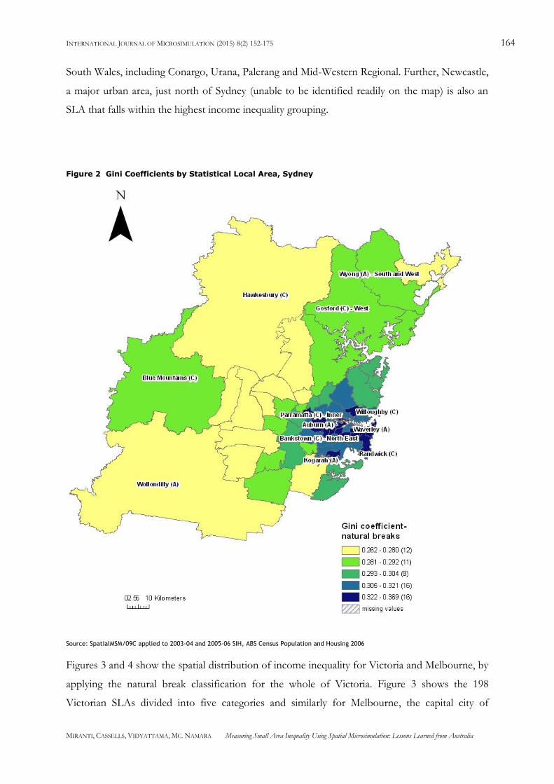
Comparing figures 1 and 2, over 50 per cent of SLAs in the highest income inequality category

(29 SLAs) lie within the capital city - Sydney (16 SLAs). SLAs with high income inequality are

mostly clustered in Sydney, with some additional high inequality SLAs scattered throughout the

rural areas of NSW. In Sydney, these SLAs run in a horizontal corridor, from east to west,

starting at the inner city suburbs of Waverley, Woollahra, Randwick, Ashfield and Strathfield, and

flowing out along the western motorway (M4) and the major train line, towards the western

suburbs of Auburn and Parramatta. For the rural areas of New South Wales, most SLAs with

high inequality are concentrated in the remote far west and north western areas of New South

Wales.

However, there are several small areas with high income inequality scattered throughout New



South Wales, including Conargo, Urana, Palerang and Mid-Western Regional. Further, Newcastle,

a major urban area, just north of Sydney (unable to be identified readily on the map) is also an

SLA that falls within the highest income inequality grouping.

Figure 2 Gini Coefficients by Statistical Local Area, Sydney

Source: SpatialMSM/09C applied to 2003-04 and 2005-06 SIH, ABS Census Population and Housing 2006

Figures 3 and 4 show the spatial distribution of income inequality for Victoria and Melbourne, by

applying the natural break classification for the whole of Victoria. Figure 3 shows the 198

Victorian SLAs divided into five categories and similarly for Melbourne, the capital city of



Victoria (Figure 4), using the same categories. As with New South Wales, the palest colour on the

map represents the areas with the lowest income inequality and the darkest colour, areas with the

highest income inequality (the highest Gini coefficient).



Figure 3 Gini Coefficients by Statistical Local Area, Victoria

Source: SpatialMSM09C applied to 2003-04 and 2005-06 SIH, ABS Census Population and Housing 2006



Figure 4 Gini Coefficients by Statistical Local Area, Melbourne

Source: SpatialMSM09C applied to 2003-04 and 2005-06 SIH, ABS Census Population and Housing 2006

Figure 4 shows that the Gini coefficients in Victoria vary between 0.247 and 0.407. Figure 4 also

shows that there are only five SLAs in Victoria that fall within the highest category of inequality,

and all of these SLAs lie within the Melbourne city statistical division. These SLAs are clustered

in the inner city area of Melbourne and include the SLAs of Melbourne – Remainder, Port

Phillips – West, Stonnington, Yarra – North and Yarra – Richmond. No SLAs in the rural areas

of Victoria fall into the highest inequality category, however, from Figure 4, we can see that there

is a large cluster of SLAs in the west of the state that fall into the second highest category of



income inequality – for example, West Wimmera, Hindmarsh, Moyne, Yarriambiack, Grampians

and Corangamite.

From these data it can be seen that in Victoria, all high inequality SLAs fall within the capital city

- Melbourne, rather than the rural areas of Victoria. However for New South Wales, the high

inequality SLAs are spread evenly between the rural areas and capital city of Sydney, with a little

over 50 per cent of high inequality SLAs found in Sydney (although it should be noted again that

the definition of ‘high inequality’ in these maps differs between the two states due to the

differences in natural breaks).

3.2. Discussion

Our small area analysis shows that some areas in NSW and Victoria have been categorised as

high inequality areas and some areas as low inequality areas. While these findings may be useful

for the purpose of policy interventions, the results and their implications should be interpreted

cautiously, due to the complexities inherent in understanding the phenomenon of high inequality

in small areas. For example, small areas with low inequality may not necessarily reflect a more

cohesive society overall or a lack of social and economic problems. A number of studies,

especially those from United States have indicated that low inequality in small areas may also

point towards segregation issues. Watson (2009) has argued that inequality may affect income

sorting that leads to income segregation at the neighbourhood level. Reardon and Bischoff (2011)

echo these results stating that lower income households tend to live in neighbourhoods with

lower incomes while higher income households tend to live within neighbourhoods with higher

incomes. Income segregation may have a negative impact on social, political and health related

outcomes. Racial tensions and increasing crime rates are examples of these unwanted outcomes

(Bayer et al. 2014; Sethi and Somathan, 2004; Watson 2009). Thus, policy makers need to

consider the balance between the potential benefits of reducing within-area inequality and the

potential adverse impact of segregation, particularly where this has implications for high levels of

neighbourhood or interregional inequality. However, it is not clear to what extent international

findings are relevant in an Australian context, and research has found more inequality between

neighbourhoods in the United States than in Australia (Hunter 2003).

In considering the characteristics associated with inequality, previous research has uncovered

factors that have been found to be determinants of inequality in Australia (see for example

Maxwell and Peter 1988; McGillivray and Peter 1991; Trendle 2005). These factors include

variables that are often associated with low income, including immigration status (Greig et al.



2003; McGillivray and Peter 1991), Indigenous status (Trendle 2005) and public housing tenancy;

as well as those that are closely related with high income, such as those with ‘high-end’

occupations, working as professionals or managers (Lyold et al. 2000) or those who have higher

educational attainment (Glaeser, et al. 2008; Maxwell and Peter 1988; Trendle 2005). McGillivray

and Peter (1991) and Trendle (2005) also examined the association between female labour force

participation and inequality. However, previous literature has shown that the relationship of

many of these variables to regional inequality is often ambiguous.

Table 4 shows the average proportion of persons in each Gini coefficient group by selected

characteristics for all of New South Wales. The groups are selected based on the natural breaks

which were applied on the maps. From Table 4 it can be seen that SLAs in the highest inequality

group are characterised by, on average, high proportions of immigrants or Culturally and

Linguistically Diverse (CALD) communities, Indigenous persons, people working as managers

and professionals, female labour force participation, people having a bachelor degree or higher,

and people living in public housing (in comparison to other Gini coefficient groups).

Table 4 Average proportion of persons in each Gini coefficient group by selected characteristics, all New South Wales, 2006 In %

Gini coefficient -

natural breaks *

Immigrants Indigenous Managers and

professionals

Female LFPR Bachelor + Public Housing

1 lowest inequality 16.37 2.61 28.56 56.25 21.43 3.42

2 12.21 3.27 30.59 51.28 20.27 3.94

3 12.73 3.06 33.97 51.12 22.13 3.54

4 15.53 4.62 39.70 52.04 25.55 3.33

5 highest inequality 23.79 7.19 46.17 54.59 33.46 4.51


Table 5 shows similar results for Victoria. In general, SLAs which fall into the highest inequality

group in Victoria, except for the proportion of population who are Indigenous (no clear pattern),

show the same pattern as in New South Wales and have high average proportions of immigrants,

people working as managers and professionals, female labour force participation, persons with a

bachelor degree or higher, and persons living in public housing.

It is interesting that the lowest inequality group in New South Wales and Victoria also has high

proportions of CALD, and high female labour force participation. This suggests that the

relationships between these variables and inequality are complex and future research is warranted.



Table 5 Average proportion of persons in each Gini coefficient group by selected characteristics, all Victoria, 2006 In %

Gini coefficient -

natural breaks *

Immigrants Indigenous Managers and

professionals

Female LFPR Bachelor + Public Housing

1 lowest inequality 17.98 0.56 25.48 59.97 22.09 1.57

2 14.29 0.71 30.11 55.43 23.71 2.47

3 14.13 1.07 33.41 51.41 21.96 2.55

4 16.99 0.53 44.22 53.17 32.62 2.08

5 highest inequality 30.18 0.31 56.23 60.79 54.69 9.69


4. CONCLUSION, LESSONS LEARNED AND POLICY IMPLICATIONS

This research has demonstrated that spatial microsimulation is an effective analytical tool that can

be used to enhance estimates of inequality at small geographic levels. The validation process

shows that our results are robust, and are closely aligned with the aggregate direct estimates

calculated from the 2005-06 Survey of Income and Housing.

The results show that although there are slight differences in terms of magnitude, the weights

give reasonable results for the vast majority of small areas in these two states, with the broad

regional rankings being very similar across both the Census and the synthetic estimates.

Our research has shown that there are clear groupings of small areas with high income inequality

in Sydney, Melbourne and rural areas of New South Wales, but not in the rural areas of Victoria.

There are several key lessons learned from this analysis of small area inequality. Firstly, the paper

has demonstrated the use of a spatial microsimulation technique to estimate inequality at small

area level that can be applied in other countries. Secondly, the findings of this research show that

inequality does differ considerably when drilling down to smaller spatial areas. For example, we

have found that most of small areas with the highest income inequality are clustered in the capital

cities but not necessarily in the rural areas.

These key lessons are important, as they can assist to inform regional policy aimed at reducing

inequality. By knowing which small areas are more unequal in regards to income, together with

the characteristics of these areas, policy makers and service providers are able to better

understand the intricacies of inequality and identify possible drivers, which can aid in more

efficient targeting of programs and policy. Nevertheless, it is important to note that examining

small area inequality does not in and of itself lead to definitive conclusions about the overall

wellbeing of an area. In particular, low inequality does not necessarily equate to better community

outcomes, nor does high inequality necessarily relate to poorer outcomes. Low inequality within



an area may be a symptom of a highly segregated population, which in turn can be associated

with interregional inequality and social unrest.

Future work in this area will concentrate on the determinants of regional inequality in order to

examine the variation of inequality across small areas in more depth, including taking into

account the spatial autocorrelation that exists between small areas. The literature suggests that the

relationships between the determinants of inequality are complex and often ambiguous. Other

planned work includes applying an inequality decomposition technique to separate ‘between‘ and

‘within‘ regional inequality and to apply the spatial microsimulation technique further in order to

model policy changes in terms of examining the impact of income distribution policies on

inequality at a small area level.

ACKNOWLEDGEMENT

This paper was funded by an Australian Research Council Discovery Grant DP664429. The

authors would like to thank the Chief Investigators on this grant, Professor Fiona Stanley,

Professor Hal Kendig, Professor Bob Stimson, Professor Ann Harding, Professor Robert Tanton

and Dr Sharon Goldfeld, as well as the Australian Bureau of Statistics for their inputs to the

broader projects under this grant.

REFERENCES

ABS (Australian Bureau of Statistics) (2006a) Income and Housing Survey (2005-06). 2nd Edition.

Basic Confidentialised Unit Record Files.

ABS (Australian Bureau of Statistics) (2006b) Household Expenditure Survey and Survey of

Income and Housing: User Guide (2003-04). Cat no. 6503.0.

ABS (Australian Bureau of Statistics) (2007a) Australian Standard Geographical Classification

(ASGC). Cat. no. 1216.0.

ABS (Australian Bureau of Statistics) (2007b) Household Income and Income Distribution. Cat

no. 6523.0.

ABS (Australian Bureau of Statistics) (2008) Australian Social Trends. Cat no. 4102.0.

Akita T (2003) ‘Decomposing regional income inequality in China and Indonesia using two-stage

nested Theil decomposition method’, The Annals of Regional Science, 37(1), 55–77.



Athanasopoulos G and Vahid F (2003) ‘Statistical Inference and Changes in Income Inequality in

Australia’, The Economic Record, 79 (247), 412-24.

Ballas D (2004) ‘Simulating Trends in Poverty and Income Inequality on the Basis of 1991 and

2001 Census Data: a Tale of Two Cities’, Area 36(2), 146-63.

Balisacan A and Fuwa N (2006) ‘Changes in spatial income inequality in Philippines: An

exploratory analysis’, in Kanbur R, Venables AJ and Wan GH (Eds.), Spatial Disparities in

Human Development: Perspective from Asia, Tokyo: University Press United Nations, 207-

32.

Bayer P, Fang H and McMillan R (2014) ‘Separate when equal? Racial inequality and residential

segregation’. Journal of Urban Economics, 82, 32-48.

Bell P (2000) GREGWT and TABLE Macros - Users Guide. Unpublished Australian Bureau of

Statistics: Canberra.

Bray JR (2001) ‘Social Indicators for Regional Australia’, Department of Families Housing

Community Services and Indigenous Affairs Policy Research Paper No. 8.

Cassells R, Miranti R and Harding A (2013) ‘Building a static spatial microsimulation model: data

preparation’, in Tanton R. and Edwards K (Eds.), Spatial Microsimulation: A Reference Guide

for Users, UK: Springer, 9-16.

Centrelink, (2015) A guide to Australian Government payments

Chin SF and Harding A (2006) ‘Regional Dimensions: Creating Synthetic Small-area Micro Data

and Spatial Microsimulation Models’, NATSEM Technical Paper No. 33.

Chotikapanich D, Flatau P, Adam M and Lloyd R (2005) Trends in Income Inequality and

Poverty in Australia in the 1990s: Regional Perspectives. Paper presented at the Australian

Social Policy Conference Sydney 20-22 July.

Elbers C, Lanjow J and Lanjow P (2003) ‘Micro-level estimation of poverty and inequality’,

Econometrica’, 71(1), 355-64.

Elbers C, Lanjow P, Mistiaen J, Ozler B and Simler K (2005) ‘Are neighbours equal? Estimating

local inequality in three developing countries’, in Kanbur R. and Venables AJ (Eds), Spatial

Inequality and Development, Oxford: Oxford University Press, 37-60.



Glaeser EL, Resseger M and Tobio K (2008) ‘Urban Inequality’, NBER Working Paper No.

14419.

Gray D, Mills JA and Zandvakili S (2003) ‘New Perspective on Canadian National and Provincial

Income Inequality’, Paper presented at the UNU-WIDER Conference on Inequality Poverty

and Human Well-being Helsinki 30-31 May.

Greig A, Lewins F and White K (2003) Inequality in Australia, Cambridge: Cambridge University

Press.

Gregory H and Hunter B (1995) ‘The Macro Economy and the Growth of Ghettos and Urban

Poverty in Australia’, Centre for Policy Research Discussion Paper No. 325.

Harding A (1997) ‘The Suffering Middle: Trends in Income Inequality in Australia’, NATSEM

Discussion Paper No. 21.

Harding A and Greenwell H (2001) ‘Trends in Income and Expenditure Inequality in the 1980s

and 1990s’, Paper presented at the 30th Annual Conference of Economists 24 September.

Hunter BH (2003) ‘Trends in Neighbourhood Inequality of Australian, Canadian, and United

States of America cities since the 1970s, Australian Economic History Review, 43(1), 22-44.

Kakwani NC and Podder N (1973) ‘On the estimation of Lorenz curves from grouped

observations’, International Economic Review, 14, 278-292.

Li Y (2005) ‘Impact of Demographic and Economic Changes on Measured Income Inequality’,

Paper presented at the Australian Social Policy Conference 2005 Sydney.

Lloyd R, Harding A and Hellwig O (2000) ‘Regional Divide? A Study of Incomes in Regional

Australia’, Australasian Journal of Regional Studies 6 (3), 271-92.

Loikkanen HA, Riihela M and Sullstrom R (2002) ‘Regional income convergence and inequality

in boom and bust: results from micro data in Finland 1971-1998 and especially during the

1990s’, Paper presented at the meeting of the ESRC Urban and Regional Economics Seminar

Group University of Central Lancashire UK 1-3 July.

Maxwell P and Peter M (1988) ‘Income Inequality in Small Regions: A Study of Australian

Statistical Division’, The Review of Regional Studies, 18 (1), 19-27.



McGillivray M and Peter M (1991) ‘Regional Income Inequality in A Developed Nation: A

Cross-Sectional Study of Australian Sub-State Regions’, The Review of Regional Studies,

21(2), 137-51.

Meagher G and Wilson S (2008) ‘Richer but More Unequal: Perceptions of Inequality in Australia

1987-2005’, Journal of Australian Political Economy, 61, 220-43.

Miranti R, Harding A, McNamara J, Ngu QV and Tanton R (2010) ‘Children with Jobless

Parents: National and Small Area Trends for Australia in the Past Decade’, Australian Journal

of Labour Economics, 13(1), 27-48.

OECD (2011) OECD Factbook 2011: Economic Environmental and Social Statistics - ISBN 978-92-64-

11150-9

OECD (2013) http://www.oecd-ilibrary.org/statistics; data extracted on 29 Apr 2013.

O’ Hagan R (1999) ‘Income Disparities and Population Movements in Victoria’, The Australasian

Journal of Regional Studies, 5(1), 87-100.

Reardon SF and Bischoff K (2011) ‘Income inequality and income segregation1’, American Journal

of Sociology, 116(4), 1092-1153.

Saunders P, Hill T and Bradbury B (2008) ‘Poverty in Australia: Sensitivity Analysis and Recent

Trends’, Social Policy Research Centre Report No. 4.

Sen A and Foster J (1997) On Economic Inequality. Oxford: Clarendon Press.

Sethi R and Somanathan R (2004) ‘Inequality and segregation’, Journal of Political Economy, 112(6),

1296-1321.

Tanton R, Harding A, and McNamara J (2013) Spatial Microsimulation Using a Generalised

Regression Model, in Tanton R. and Edwards, K.L (Eds), Spatial Microsimulation: A Reference

Guide for Users, Netherlands: Springer, 87-103.

Tarozzi A and Deaton A (2009) ‘Using Census and Survey Data to Estimate Poverty and

Inequality for Small Areas’, The Review of Economics and Statistics, 91(4), 773-92.

Trendle B (2005) ‘Sources of Regional Income Inequality: An Examination of Small Regions in

Queensland’, Review of Urban and Regional Development Studies, 17(1), 35-50.

http://www.oecd-ilibrary.org/statistics



Thapa PJ (2004) ‘On the risk of unemployment: A comparative Assessment of the Labour

Market Success of Migrants in Australia’, Australian Journal of Labour Economics, Vol.7, Issue 2,

199-229.

Vu QN, Harding A, Tanton R, Nepal B and Vidyattama Y (2008) Advance Australia Fair? AMP.

NATSEM Income and Wealth Report, No. 20.

Watson T (2009) ‘Inequality and the measurement of residential segregation by income in

American neighborhoods’, Review of Income and Wealth, 55(3), 820-844.

Wodon Q and Yitzhaki S (2003) ‘The effect of using grouped data on the estimation of the Gini

income elasticity’, Economics Letters, 78(2), 153-159.

Williamson J (1965) ‘Regional Inequality and the Process of National Development’. Economic

Development and Cultural Change, 13(4), 3-47.

Wilkinson R (2006) The Impact of Inequality: How to Make Sick Societies Healthier. New York:

New Press.

1 Gini coefficients are calculated for persons using household disposable income.

2 There is a large literature on the estimation of Gini coefficients from grouped data. See for example Kakwani and Podder (1973) and Wodon

and Yitzhaki (2003).

3. Only 0.79 per cent of the total Australian population in 2006 are lost in the reweighting process.

Date post:	09-Mar-2018
Category:	Documents
Upload:	dangtuong
View:	224 times
Download:	4 times

Measuring Small Area Inequality Using Spatial ... · PDF fileMeasuring Small Area Inequality...

Documents